Embed Size (px)
Citation preview

—
COLLEGE OF SCIENCE AND TECHNOLOGY
APPLICATIONS OF CONFORMAL MAPPINGS TOTHE FLUID FLOW
Master of Science
in
Applied Mathematics
2018

COLLEGE OF SCIENCE AND TECHNOLOGY
SCHOOL OF SCIENCES
DEPARTMENT OF MATHEMATICS
APPLICATIONS OF CONFORMAL MAPPINGS TOTHE FLUID FLOW
By
NYANDWI BoscoStudent Number: 217124283
Thesis Submitted in Partial Fulfillment of the Academic
Requirements for the Degree of
Master of Science
in
Applied Mathematics
Option of Mathematical Modeling and Scientific Computing
Supervisor: Prof. Rickard Bogvad
Kigali, Rwanda
April, 2018
i
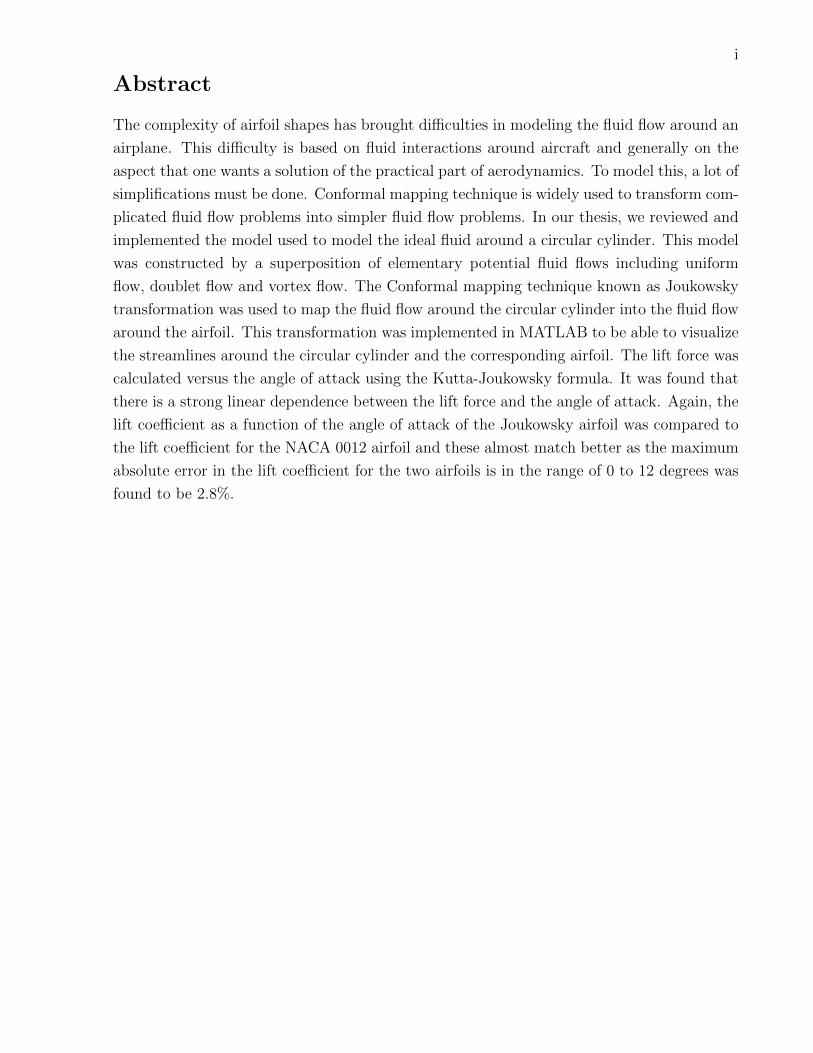
Abstract
The complexity of airfoil shapes has brought difficulties in modeling the fluid flow around an
airplane. This difficulty is based on fluid interactions around aircraft and generally on the
aspect that one wants a solution of the practical part of aerodynamics. To model this, a lot of
simplifications must be done. Conformal mapping technique is widely used to transform com-
plicated fluid flow problems into simpler fluid flow problems. In our thesis, we reviewed and
implemented the model used to model the ideal fluid around a circular cylinder. This model
was constructed by a superposition of elementary potential fluid flows including uniform
flow, doublet flow and vortex flow. The Conformal mapping technique known as Joukowsky
transformation was used to map the fluid flow around the circular cylinder into the fluid flow
around the airfoil. This transformation was implemented in MATLAB to be able to visualize
the streamlines around the circular cylinder and the corresponding airfoil. The lift force was
calculated versus the angle of attack using the Kutta-Joukowsky formula. It was found that
there is a strong linear dependence between the lift force and the angle of attack. Again, the
lift coefficient as a function of the angle of attack of the Joukowsky airfoil was compared to
the lift coefficient for the NACA 0012 airfoil and these almost match better as the maximum
absolute error in the lift coefficient for the two airfoils is in the range of 0 to 12 degrees was
found to be 2.8%.

ii
Acknowledgments
I would like to thank my adviser Prof. Rickard Bogvad for his encouragement and guidance
to me during the process of this dissertation. Also, I would like to thank my friends and
colleagues at University of Rwanda who provided some good advices that motivated me.
My gratitude is also addressed to the staff of University of Rwanda, all the lecturers who
contributed to my academic studies. I finally wish to express my gratitude to my family
members especially my Mother and my Grand brother for their support they provided to
me.
iii
Declaration
I, NYANDWI Bosco, hereby declare that this thesis was conducted at University of
Rwanda under the supervision of Prof. Rickard Bogvad and is my original work and
has never been submitted anywhere else for academic purposes.
Student: NYANDWI Bosco
Signature:

iv

Contents
Abstract . . . . . . . . . . . . . . . . . . . . . . . . . . . . . . . . . . . . . . . . . i
Acknowledgments . . . . . . . . . . . . . . . . . . . . . . . . . . . . . . . . . . . . ii
Declaration . . . . . . . . . . . . . . . . . . . . . . . . . . . . . . . . . . . . . . . iii
Contents v
List of Tables vii
1 General Introduction 1
1.1 Introduction . . . . . . . . . . . . . . . . . . . . . . . . . . . . . . . . . . . . 1
1.2 Airplanes . . . . . . . . . . . . . . . . . . . . . . . . . . . . . . . . . . . . . 2
1.2.1 Description of Airplane Wings . . . . . . . . . . . . . . . . . . . . . . 2
1.3 Fluid Dynamics . . . . . . . . . . . . . . . . . . . . . . . . . . . . . . . . . . 5
1.3.1 Fluid Velocity . . . . . . . . . . . . . . . . . . . . . . . . . . . . . . 5
1.3.2 The Continuity Equation: Mass Conservation . . . . . . . . . . . . . 9
1.3.3 Some Multivariate Calculus . . . . . . . . . . . . . . . . . . . . . . . 10
1.4 Stream Function . . . . . . . . . . . . . . . . . . . . . . . . . . . . . . . . . 11
1.4.1 Velocity Potential and Stream Function . . . . . . . . . . . . . . . . 12
1.5 Analytic and Harmonic Functions . . . . . . . . . . . . . . . . . . . . . . . . 13
1.5.1 Complex Analytic Functions . . . . . . . . . . . . . . . . . . . . . . . 14
1.5.2 Singularities . . . . . . . . . . . . . . . . . . . . . . . . . . . . . . . . 15
1.5.3 Conformal Transformations . . . . . . . . . . . . . . . . . . . . . . . 16
1.6 Problem Statement . . . . . . . . . . . . . . . . . . . . . . . . . . . . . . . . 16
1.7 Objectives . . . . . . . . . . . . . . . . . . . . . . . . . . . . . . . . . . . . . 19
1.7.1 Scope of the Study . . . . . . . . . . . . . . . . . . . . . . . . . . . . 19
1.7.2 Significance of the Study . . . . . . . . . . . . . . . . . . . . . . . . 19
1.8 Outline . . . . . . . . . . . . . . . . . . . . . . . . . . . . . . . . . . . . . . 19
2 Literature Review 21
2.1 Modeling the Fluid around an Airplane Wing . . . . . . . . . . . . . . . . . 21
2.1.1 Uniform Flow . . . . . . . . . . . . . . . . . . . . . . . . . . . . . . . 21
2.1.2 Source and Sink Flow . . . . . . . . . . . . . . . . . . . . . . . . . . . 22
v

vi CONTENTS
2.1.3 A Combination of a Uniform Flow with a Source and Sink Flow . . . 24
2.1.4 Doublet flow . . . . . . . . . . . . . . . . . . . . . . . . . . . . . . . . 25
2.1.5 Superposition of a Uniform Flow and a Doublet Flow . . . . . . . . . 26
2.1.6 Vortex Flow . . . . . . . . . . . . . . . . . . . . . . . . . . . . . . . . 28
2.1.7 Lifting Flow over a Cylinder . . . . . . . . . . . . . . . . . . . . . . . 29
2.1.8 Lift and Drag around two Dimensional Shapes . . . . . . . . . . . . . 31
3 Methodology 33
3.1 The Conformal Mapping Technique . . . . . . . . . . . . . . . . . . . . . . . 33
3.2 Mapping from a Circular Cylinder to an Airfoil with the Joukowsky Transfor-
mation . . . . . . . . . . . . . . . . . . . . . . . . . . . . . . . . . . . . . . . 34
4 Results and Analysis 39
4.1 Computing the Streamlines around an Airfoil and Lift calculation . . . . . . 39
5 Conclusion 45
A MATLAB Codes 47
REFERENCES . . . . . . . . . . . . . . . . . . . . . . . . . . . . . . . . . . . . . 47
Bibliography 53

List of Tables
4.1 Summary of results for lift force calculation. . . . . . . . . . . . . . . . . . . 42
4.2 Summary of results for lift coefficient calculation. . . . . . . . . . . . . . . . 43
4.3 Summary of results for lift coefficient calculation. . . . . . . . . . . . . . . . 43
vii

Chapter 1
General Introduction
1.1 Introduction
Conformal mapping have been used in studying the airflow around an airplane. Due to the
complexity of the flow around it, a lot of simplifications must be done. This difficulty is
based on fluid interactions around aircraft and generally on the aspect that one wants a
solution of the practical part of aerodynamics. The most useful technique to transform the
complicated airflow problem to a simple problem is a conformal mapping which is used as
an intermediate step that gives a way of solving the problem with simpler geometry. An air
plane wing is defined as the cross sectional shape of an object designed to generate lift when
moving through a fluid. Basically, an airplane wing generates lift by diverting the motion of
fluid flowing over its surface in a downward direction, resulting in an upward reaction force
by Newton’s third law [14]. A quantitative method of analyzing fluid flow and lift is needed
to understand the design of applicable systems.
This method, known as conformal mapping, will be the main emphasis of this thesis.
Our thesis goal will be to provide students with a deep understanding of multivariable calcu-
lus and an understanding of complex variable mathematics with an important application.
Conformal mapping is a mathematical technique in which complicated geometries can be
transformed by a mapping function into simpler geometries which still preserve both the an-
gles and orientation of the original geometry [1]. Using this technique, the fluid flow around
the geometry of an airplane wing can be analyzed as the flow around a cylinder whose sym-
metry simplifies the needed computations. Since the functions that describe the fluid flow
satisfy the equation of Laplace, the conformal mapping method allows for lift calculations on
the cylinder to be equated to those on the corresponding airplane wing.
This thesis focuses on constructing the two-dimensional fluid flow around the airplane
wing using the conformal mapping technique. We will now introduce some of the concepts
1
2 CHAPTER 1. GENERAL INTRODUCTION
that will be used in this thesis, so as to give an idea of which techniques will be used to solve
our problem. We will provide a description and the characteristics of an airplane wing. Next,
we will construct a physical model used to represent the inviscid, incompressible fluid flow
around an airplane wing (airfoil), and explain the theory behind conformal mapping. We
will then use a special application of conformal mapping called Joukowsky transformation, to
map the solution for flow around a circular cylinder to the solution for flow around airplane
wings. We will implement this conformal mapping transformation to compute the fluid flow
and lift around Joukowsky airfoil.
1.2 Airplanes
1.2.1 Description of Airplane Wings
It is very important to give the geometrical description of the wing of an aircraft in the
beginning of our journey of constructing the fluid flow around it.
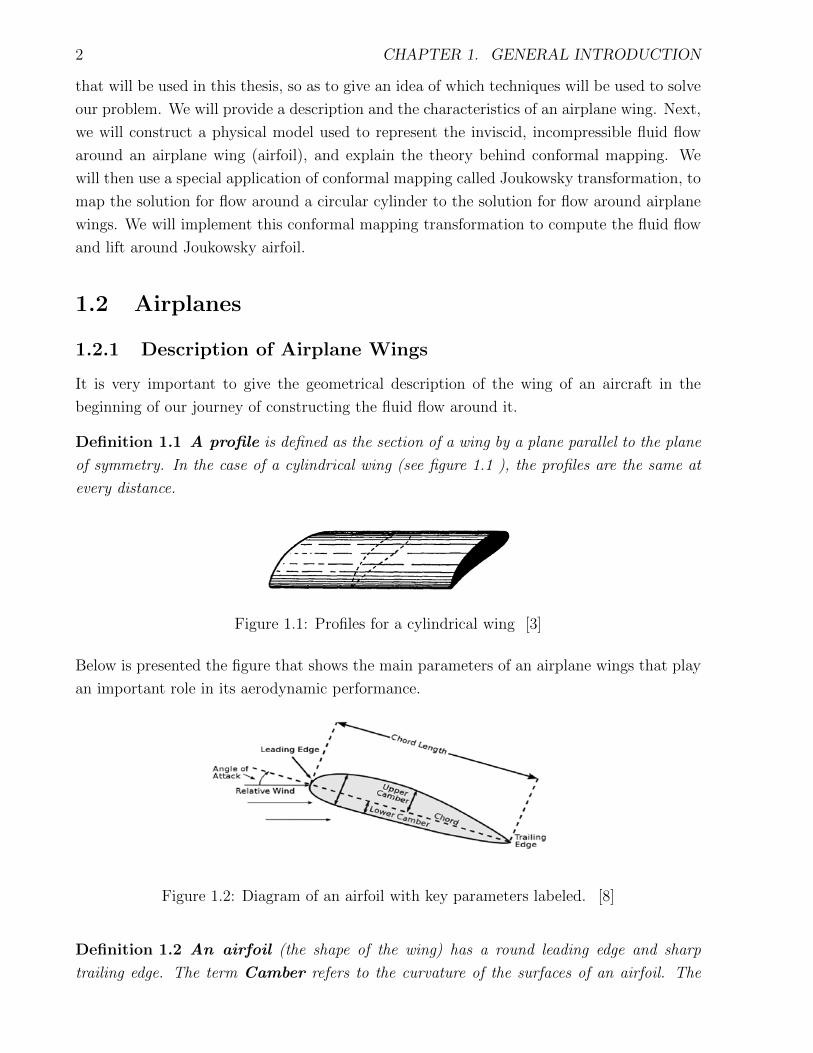
Definition 1.1 A profile is defined as the section of a wing by a plane parallel to the plane
of symmetry. In the case of a cylindrical wing (see figure 1.1 ), the profiles are the same at
every distance.
Figure 1.1: Profiles for a cylindrical wing [3]
Below is presented the figure that shows the main parameters of an airplane wings that play
an important role in its aerodynamic performance.
Figure 1.2: Diagram of an airfoil with key parameters labeled. [8]
Definition 1.2 An airfoil (the shape of the wing) has a round leading edge and sharp
trailing edge. The term Camber refers to the curvature of the surfaces of an airfoil. The

1.2. AIRPLANES 3
Figure 1.3: Detailed drawing of an airfoil with main parameters labeled. [7]
airfoil shown in figure 1.3 is a positive cambered airfoil because the mean camber line is located
above the chord line. The mean camber line (3) is a line drawn halfway between the upper
and lower surfaces. The mean camber of an airfoil may be considered as the curvature of the
median line (mean camber line) of the airfoil. The shape of the mean camber is important in
determining the aerodynamic characteristics of an airfoil section. The chord line (1) is a
straight line connecting the leading and trailing edges of the airfoil. The chord line connects
the ends of the mean camber line. The chord (2) is the length of the chord line from
leading edge to trailing edge and is the characteristic longitudinal dimension of an airfoil.
Maximum camber (4) (displacement of the mean camber line from the chord line) and
where it is located (expressed as fractions or percentages of the basic chord) help to define the
shape of the mean camber line. The maximum thickness (5) of an airfoil and where it
is located (expressed as a percentage of the chord) help define the airfoil shape, and hence its
performance. The leading edge radius (6) of the airfoil is the radius of curvature given
the leading edge shape. We are in particular interested in the length of the chord, the angle
of attack and the mean camber line.
Figure 1.4: Angle of attack denoted by α. [4]
Definition 1.3 The angle of attack denoted by α is the angle between the direction of
4 CHAPTER 1. GENERAL INTRODUCTION
the motion and the direction of the chord line.
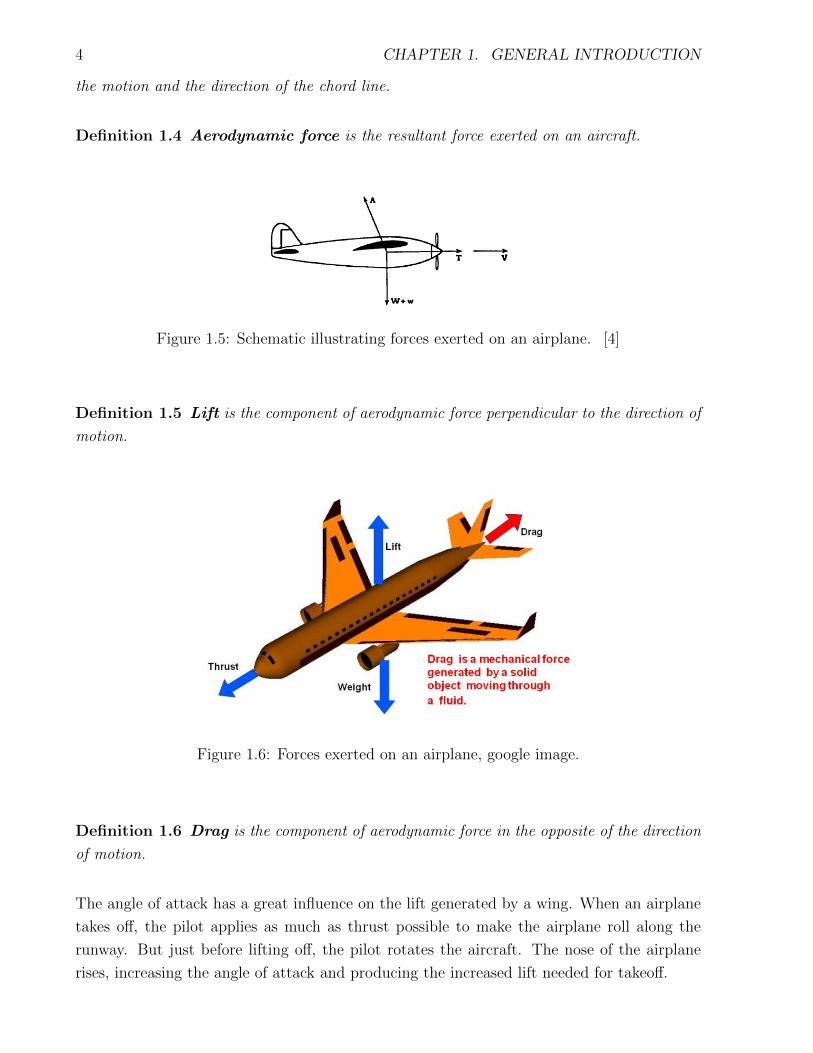
Definition 1.4 Aerodynamic force is the resultant force exerted on an aircraft.
Figure 1.5: Schematic illustrating forces exerted on an airplane. [4]
Definition 1.5 Lift is the component of aerodynamic force perpendicular to the direction of
motion.
Figure 1.6: Forces exerted on an airplane, google image.
Definition 1.6 Drag is the component of aerodynamic force in the opposite of the direction
of motion.
The angle of attack has a great influence on the lift generated by a wing. When an airplane
takes off, the pilot applies as much as thrust possible to make the airplane roll along the
runway. But just before lifting off, the pilot rotates the aircraft. The nose of the airplane
rises, increasing the angle of attack and producing the increased lift needed for takeoff.

1.3. FLUID DYNAMICS 5
Figure 1.7: Forces exerted on an airplane can be resolved into two components: Lift and
Drag. [4]
1.3 Fluid Dynamics
Definition 1.7 A fluid is defined as any material that exhibits deformation under the action
of forces.
Definition 1.8 A flow is a deformation of a material that increases continuously without
limit under the action of forces, however small.
Actual fluids are classified into two categories: gas and liquids. Since a gas such as atmo-
spheric air fills any closed space to which has access, it is therefore classified as compressible
fluid. A liquid is regarded as incompressible because a liquid has a constant pressure and
temperature and takes a definite volume and when placed in an open vessel will take under
the action of gravity the form of the lower part of the vessel and will be bounded above by
a horizontal free surface.
Definition 1.9 Viscous fluid flows refer to real flows which exhibit the effects of trans-
ports phenomena (the phenomena of mass diffusion, viscosity and thermal conductivity).
Definition 1.10 A fluid flow is called an inviscid flow if it is assumed to involve no
friction, thermal conductivity or diffusion.
But in nature such flows do not exist, however, there are many practical aerodynamic flows
where the influence of the transport phenomena is small, and we can model the flow as being
inviscid.
1.3.1 Fluid Velocity
One can define a fluid particle as consisting of the fluid contained in an infinitesimal volume,
that is to say, a volume whose size may be considered so small that for the particular purpose

6 CHAPTER 1. GENERAL INTRODUCTION
in hand its linear dimensions are negligible. We can then treat a fluid particle as a geometrical
point for the particular purpose of discussing its velocity and acceleration. If we consider,
the particle which at time t is at the point P , defined by the vector s =−→OP at time t1, this
particle will have moved to the point Q, defined by the vector s1 =−→OQ (see figure1.8).
Figure 1.8: The particle at the point P at time t moves the point Q at time t1 [4].
Definition 1.11 The velocity of the particle at P is then defined by the vector
~V = limt1→t
s1 − st1 − t
=ds
dt.
Thus the velocity ~V is a function of s and t, say ~V = g(s, t). If the form of the function g is
known then we know the motion of the fluid.
Definition 1.12 A steady flow is a flow with a constant velocity. It means that∂~V
∂t= 0.
Definition 1.13 A streamline is a curve drawn in the fluid that maps t 7→ s(t), in R3 so
that its tangent at each point is in the direction of the fluid velocity ~V at that point, i.e.,
~V × d~s = 0, (1.1)
where d~s =~idx+~jdy + ~kdz, stands for a line element in the Cartesian frame and~V = u~i+ v~j + w~k, where u, v, w are the velocity components.
The expansion of equation (1.1) (under the hypothesis that u, v, w are non-zero) follows below
~V × d~s = 0 (1.2)
⇔
∣∣∣∣∣∣∣~i ~j ~k
u v w
dx dy dz
∣∣∣∣∣∣∣ = 0
⇔
vdz − wdy = 0
udz − wdx = 0
udy − vdx = 0
1.3. FLUID DYNAMICS 7
⇔
udz = wdx
vdz = wdy
udy = vdx
⇔
dz
w=dy
vdz
w=dx
udy
v=dx
u
⇔ dx
u=dy
v=dz
w. (1.3)
The differential equations (1.3) when solved give the family of streamlines at any instant.
When the flow is steady the streamlines will have the same form at all t. These equations
may also be formulated as ds = λ~V , for some non-zero λ = λ(t) ∈ R, and this formulation
is then valid for a flow in two dimensional space too (in this case the first two equations of
(1.3) will be true). Note that streamlines cannot intersect one another, except at points (and
times) when ~V is either singular or zero, by standard properties of differential equations.
Definition 1.14 Stream tube is the surface formed instantaneously by all streamlines which
pass through a given closed curve in the fluid.
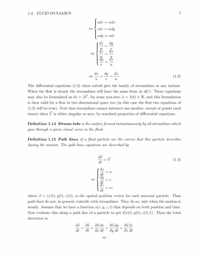
Definition 1.15 Path lines of a fluid particle are the curves that this particle describes
during the motion. The path lines equations are described by
d~s
dt= ~V (1.4)
⇔
dx
dt= u
dy
dt= v
dz
dt= w,
where ~s = (x(t), y(t), z(t)), is the spatial position vector for each material particle. Thus
path lines do not, in general, coincide with streamlines. They do so, only when the motion is
steady. Assume that we have a function s(x, y, z, t) that depends on both position and time.
Now evaluate this along a path line of a particle to get ~s(x(t), y(t), z(t), t). Then the total
derivative is
d~s
dt=∂~s
∂t+∂~s
∂x
dx
dt+∂~s
∂y
dy
dt+∂~s
∂z
dz
dt
⇔
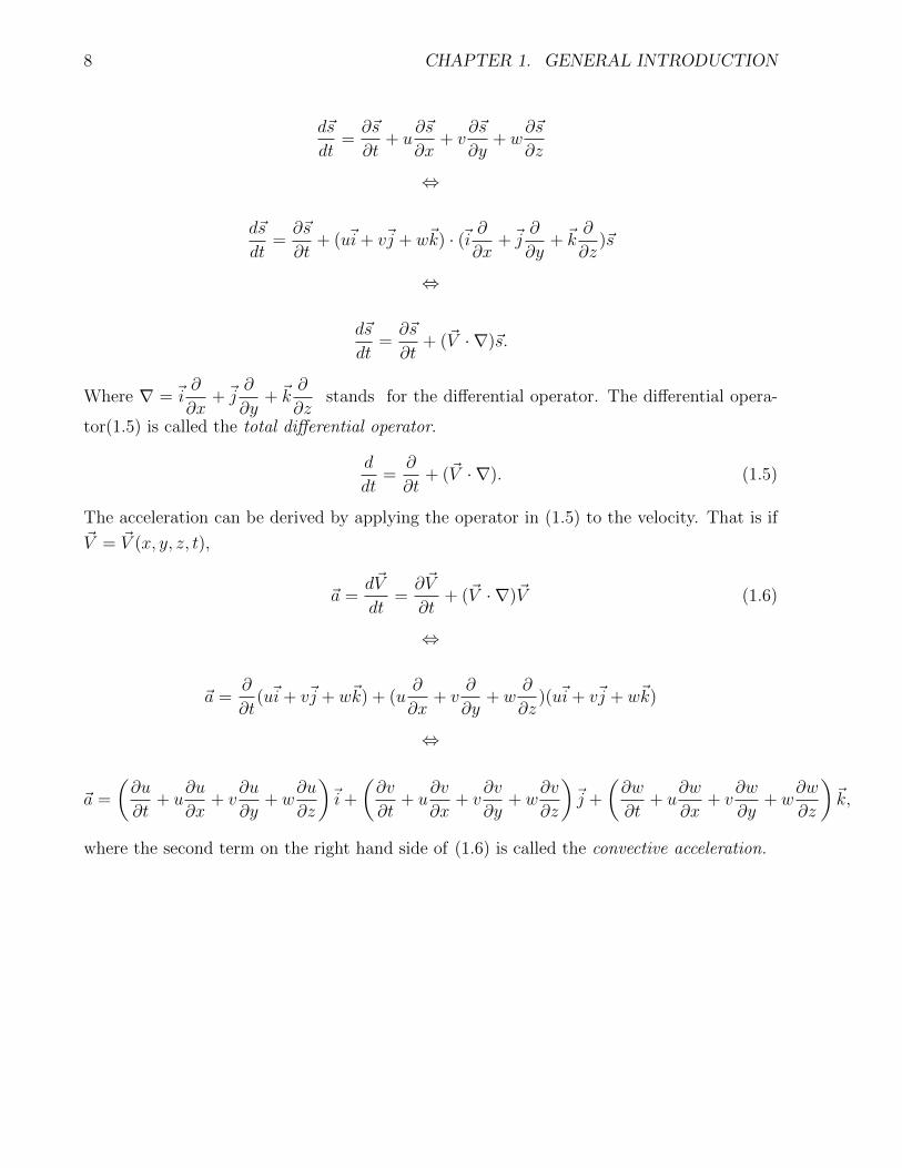
8 CHAPTER 1. GENERAL INTRODUCTION
d~s
dt=∂~s
∂t+ u
∂~s
∂x+ v
∂~s
∂y+ w
∂~s
∂z
⇔
d~s
dt=∂~s
∂t+ (u~i+ v~j + w~k) · (~i ∂
∂x+~j
∂
∂y+ ~k
∂
∂z)~s
⇔
d~s
dt=∂~s
∂t+ (~V · ∇)~s.
Where ∇ = ~i∂
∂x+~j
∂
∂y+ ~k
∂
∂zstands for the differential operator. The differential opera-
tor(1.5) is called the total differential operator.
d
dt=
∂
∂t+ (~V · ∇). (1.5)
The acceleration can be derived by applying the operator in (1.5) to the velocity. That is if~V = ~V (x, y, z, t),
~a =d~V
dt=∂~V
∂t+ (~V · ∇)~V (1.6)
⇔
~a =∂
∂t(u~i+ v~j + w~k) + (u
∂
∂x+ v
∂
∂y+ w
∂
∂z)(u~i+ v~j + w~k)
⇔
~a =
(∂u
∂t+ u
∂u
∂x+ v
∂u
∂y+ w
∂u
∂z
)~i+
(∂v
∂t+ u
∂v
∂x+ v
∂v
∂y+ w
∂v
∂z
)~j +
(∂w
∂t+ u
∂w
∂x+ v
∂w
∂y+ w
∂w
∂z
)~k,
where the second term on the right hand side of (1.6) is called the convective acceleration.
1.3. FLUID DYNAMICS 9
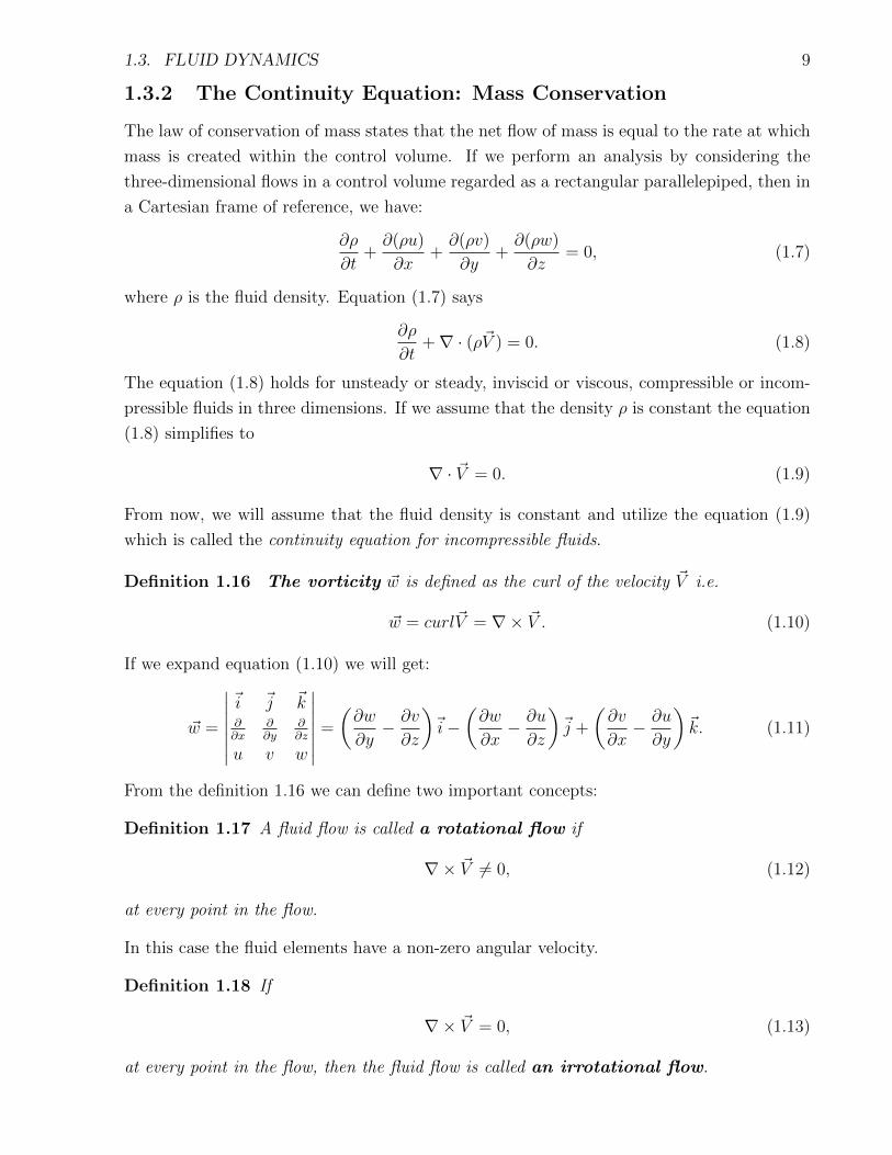
1.3.2 The Continuity Equation: Mass Conservation
The law of conservation of mass states that the net flow of mass is equal to the rate at which
mass is created within the control volume. If we perform an analysis by considering the
three-dimensional flows in a control volume regarded as a rectangular parallelepiped, then in
a Cartesian frame of reference, we have:
∂ρ
∂t+∂(ρu)
∂x+∂(ρv)
∂y+∂(ρw)
∂z= 0, (1.7)
where ρ is the fluid density. Equation (1.7) says
∂ρ
∂t+∇ · (ρ~V ) = 0. (1.8)
The equation (1.8) holds for unsteady or steady, inviscid or viscous, compressible or incom-
pressible fluids in three dimensions. If we assume that the density ρ is constant the equation
(1.8) simplifies to
∇ · ~V = 0. (1.9)
From now, we will assume that the fluid density is constant and utilize the equation (1.9)
which is called the continuity equation for incompressible fluids.
Definition 1.16 The vorticity ~w is defined as the curl of the velocity ~V i.e.
~w = curl~V = ∇× ~V . (1.10)
If we expand equation (1.10) we will get:
~w =
∣∣∣∣∣∣∣~i ~j ~k∂∂x
∂∂y
∂∂z
u v w
∣∣∣∣∣∣∣ =
(∂w
∂y− ∂v
∂z
)~i−
(∂w
∂x− ∂u
∂z
)~j +
(∂v
∂x− ∂u
∂y
)~k. (1.11)
From the definition 1.16 we can define two important concepts:
Definition 1.17 A fluid flow is called a rotational flow if
∇× ~V 6= 0, (1.12)
at every point in the flow.
In this case the fluid elements have a non-zero angular velocity.
Definition 1.18 If
∇× ~V = 0, (1.13)
at every point in the flow, then the fluid flow is called an irrotational flow.

10 CHAPTER 1. GENERAL INTRODUCTION
In this case, the fluid elements have no angular velocity. In two dimensions, equation (1.13)
becomes:
∂v
∂x− ∂u
∂y= 0. (1.14)
We will frequently use equation (1.14) in the next sections.
Definition 1.19 The Bernoulli equation for an incompressible inviscid fluid is given
below: p+ 12ρ~V 2 = const, where p is the pressure, ρ the density, ~V the fluid velocity and ~V 2
the square of the velocity.
It is clear to see that the pressure decreases as the velocity increases and conversely, the
velocity decreases as the pressure increases. This is the physical meaning of the Bernoulli
equation [10]. This equation will be used in section 2.1.8 to explain how the lift force is
generated around a spinning cylinder.
1.3.3 Some Multivariate Calculus
To define the circulation, let us start by stating the theorems of Green and Stokes.
Theorem 1.1 (Green’s Theorem): Let C be a positively oriented, piecewise, smooth,
simple closed curve in the plane and let D be the region bounded by C.
Let F (x, y) = P (x, y)~i+Q(x, y)~j, be a vector field of class C1. Then∮C
Pdx+Qdy =
∫∫D
(∂Q
∂x− ∂P
∂y
)dA. (1.15)
And the vector form of 1.1 is ∮C
F · ds =
∫∫D
(∇× F ) · kdA, (1.16)
where k is the unit outward normal vector.
Theorem 1.2 (Stokes’ theorem): Let S be an oriented piecewise-smooth surface that is
bounded by a simple, closed, piecewise-smooth boundary curve C with positive orientation.
Let F be a vector field whose components have continuous partial derivatives on an open
region in <3 that contains S.Then∮C
F · dr =
∫∫S
(∇× F ) · dS [9]. (1.17)
Definition 1.20 Circulation: Let C be a closed curve in a fluid. Let ~V and ds be the
velocity and the line segment of C, respectively. The circulation denoted by Γ, is defined as
the curve integral
Γ =
∮C
~V · ds. (1.18)

1.4. STREAM FUNCTION 11
The circulation is related to the vorticity as follows
Γ =
∮C
~V · ds =
∫∫S
(∇× ~V ) · dS, (1.19)
thus the circulation about a curve is equal to the vorticity integrated over any open surface
S bounded by C [10]. This is an immediate consequence of Theorem 1.2; so we get the
following corollary:
Corollary 1.1 If the flow is irrotational everywhere within the contour of integration over
any surface bounded by C then the circulation Γ = 0.
1.4 Stream Function
Consider a two-dimensional motion of air considered as an incompressible fluid. Let A be a
Figure 1.9: Two dimensional flow. [4]
fixed point in the plane of motion, P an arbitrary point and ABP and ACP two curves in
the plane joining A to P . Assume that there is no air created or destroyed within the region
R bounded by the two curves. And now, the condition of continuity can be expressed in the
following form. The rate at which air flows into the region R from right to left across the
curve ABP is equal to the rate at which it flows out from right to the left across the curve
ACP . The flux from right to left across ACP is equal to the flux from right to the left across
any curve joining A to P . Once the base point A has been fixed this flux therefore depends
solely on the position of P, and the time t. If we denote the flux by ψ, it is a function of
P , and the time t. The function ψ = ψ(x, y, t) is called the stream function (where in
Cartesian coordinates P = (x, y)). The existence of this function is merely a consequence of
the assertion of the continuity of incompressible air.
Let ψ1, ψ2 be the values of the stream functions at the points P1 and P2 respectively, From
the same principle, the flux across AP2 is equal to the flux across AP1 plus that P1P2. Hence
the flux across P1P2 equals ψ2−ψ1. It follows from this that if we take a different base point,
B say, the stream function merely changes by the flux from right to left across BA . Hence
the steam function is uniquely determined up to an additive constant. Moreover, if P1 and P2
are points of the same streamline, there is clearly no flux over the streamline between P1 and
P2, and thus ψ2−ψ1 = 0. Therefore the stream function is constant along a streamline. The

12 CHAPTER 1. GENERAL INTRODUCTION
Figure 1.10: Two dimensional flow. [4]
equations of the streamlines are therefore obtained from ψ = c, by giving arbitrary values to
the constant c. When the motion is steady, the streamline pattern is fixed. When the motion
is not steady, the pattern changes from instant to instant with t [4].
1.4.1 Velocity Potential and Stream Function
Consider a two dimensional velocity field in the form
~V = u(x, y, t)~i+ v(x, y, t)~j. (1.20)
If the vector field is irrotational then by (1.14)∂v
∂x=∂u
∂y, and by (1.15)
∮Cudx + vdy = 0,
along any closed curve C. Hence choosing a base point A, and letting P = (x, y) be a variable
point, the curve integral along a curve Γ between A and P ,
∮Γ
udx+ vdy, (1.21)
does not depend on which curve Γ we use. So we can define
φ(x, y, t) = −∫ P
A
udx+ vdy. (1.22)
Note that
u = −∂φ∂x, v = −∂φ
∂y. (1.23)
The function φ is called the velocity potential and we have ~V = −∇φ, that is up to a sign
change, the gradient of φ.
Now consider the stream function. If Γ is curve from A to P , it is defined as the flux across
Γ, and this flux ( at a point on the curve) is given as the scalar product of ~V and the normal
(−dy, dx) = −dy~i+ dx~j to the curve, and hence as the curve integral∮Γ
vdx− udy. (1.24)
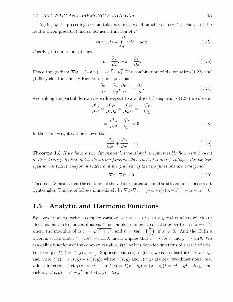
1.5. ANALYTIC AND HARMONIC FUNCTIONS 13
Again, by the preceding section, this does not depend on which curve Γ we choose (if the
fluid is incompressible) and so defines a function of P ,
ψ(x, y, t) =
∫ P
A
vdx− udy. (1.25)
Clearly , this function satisfies
v =∂ψ
∂x, −u =
∂ψ
∂y. (1.26)
Hence the gradient ∇ψ = (−v, u) = −v~i + u~j. The combination of the equations(1.23) and
(1.26) yields the Cauchy Riemann type equations
∂φ
∂x=∂ψ
∂y,∂ψ
∂x= −∂φ
∂y. (1.27)
And taking the partial derivatives with respect to x and y of the equations (1.27) we obtain:
∂2φ
∂x2=
∂2ψ
∂x∂y=
∂2ψ
∂y∂x= −∂
2φ
∂2y.
⇒ ∂2φ
∂x2+∂2φ
∂y2= 0. (1.28)
In the same way, it can be shown that
∂2ψ
∂x2+∂2ψ
∂y2= 0. (1.29)
Theorem 1.3 If we have a two dimensional, irrotational, incompressible flow with φ equal
to its velocity potential and ψ its stream function then each of φ and ψ satisfies the Laplace
equation in (1.28) and/or in (1.29) and the gradient of the two functions are orthogonal:
∇φ · ∇ψ = 0. (1.30)
Theorem 1.3 means that the contours of the velocity potential and the stream function cross at
right-angles. The proof follows immediately by ∇φ ·∇ψ = (−u,−v) ·(v,−u) = −uv+uv = 0.
1.5 Analytic and Harmonic Functions
By convention, we write a complex variable as z = x + iy with x, y real numbers which are
identified as Cartesian coordinates. The complex number z can also be written as z = reiθ,
where the modulus of is r =√x2 + y2, and θ = tan−1
(yx
), if x 6= 0. And the Euler’s
theorem states that eiθ = cos θ + i sin θ, and it implies that x = r cos θ, and y = r sin θ. We
can define functions of the complex variable, f(z) as it is done for functions of a real variable.
For example f(z) = z2, f(z) =1
z. Suppose that f(z) is given, we can substitute z = x+ iy,
and write f(z) = u(x, y) + iv(x, y), where u(x, y) and v(x, y) are real two-dimensional real
valued functions. Let f(z) = z2, then f(z) = f(x + iy) = (x + iy)2 = x2 − y2 − 2ixy, and
yielding u(x, y) = x2 − y2, and v(x, y) = 2xy.

14 CHAPTER 1. GENERAL INTRODUCTION
1.5.1 Complex Analytic Functions
Consider the complex valued function f(z) = u(x, y) + iv(x, y), where z = x + iy. Pro-
vided that u(x, y) and v(x, y) have continuous partial derivatives, the Cauchy Riemann
Equations are defined as follows:
∂u
∂x=∂v
∂y,∂u
∂y= −∂v
∂x. (1.31)
The Cauchy Riemann equations in polar coordinates can be written as:
∂u
∂r=
1
r
∂v
∂θ,∂v
∂r= −1
r
∂u
∂θ. (1.32)
where x = r cos θ, y = r sin θ, r2 = x2+y2, and tan θ =y
x[3]. (Here we assume r 6= 0, x 6= 0).
Theorem 1.4 The function f(z) = u(x, y)+iv(x, y), is differentiable at the point z = x+iy,
of the region in the complex plane if and only if the partial derivatives∂u
∂x,∂u
∂y,∂v
∂x,∂v
∂y, are
continuous and satisfy the Cauchy Riemann equations at z = x+ iy.
Definition 1.21 A function is said to be analytic at a point z0 if f(z) is differentiable
in a neighborhood of z0.
The function f(z) is said to be analytic in a region D if it is analytic at every point in
the region [3]. The points at which is not analytic are called singularities. If f(z) and g(z)
are analytic functions, then so are
1. f(z)± g(z)
2. f(z) · g(z)
3. f(z)/g(z), (if g(z) is non-zero in D)
4. f (g(z))
It follows that polynomial are analytic functions in D. Power series within their circles of
convergence are also analytic functions.The real and imaginary parts of an analytic function
are called conjugate functions. Note that they related to each other by the Cauchy-
Riemann equations.
Theorem 1.5 We can construct a function
Θ(z) = φ(x, y) + iψ(x, y), (1.33)
called the complex velocity potential, using the velocity potential φ(x, y) and the stream func-
tion φ(x, y). It is an analytic function.

1.5. ANALYTIC AND HARMONIC FUNCTIONS 15
Proof:
Since φ and ψ are continuous functions of their argument z = x+ iy, so is Θ. By (1.27)
∂φ
∂x=∂ψ
∂y,∂ψ
∂x= −∂φ
∂y.
That means that Θ satisfies the Cauchy-Riemann Equations in (1.31) and so the theorem is
a consequence of the characterization of analytic functions in theorem 1.4.
Note that φ, ψ satisfy Laplace’s equation (1.28). This is always true of the real or imaginary
part of an analytic function, and such functions are called harmonic.
Proposition 1.1 For the functions φ and ψ satisfying the Cauchy Riemann equations, the
level curves φ = constant, and ψ = constant, meet at right angles to each other.
Proof:
The gradient
(∂φ
∂x,∂φ
∂y
), at P = (x, y) is orthogonal to the level curve φ through P . Similarly
the level curve of ψ through P is orthogonal to(∂ψ
∂x,∂ψ
∂y
).
But, by the Cauchy Riemann equations, these gradients are orthogonal:(∂ψ
∂x,∂ψ
∂y
)=
(−∂φ∂y,∂φ
∂x
), and so
(∂ψ
∂x,∂ψ
∂y
)·(−∂φ∂y,∂φ
∂x
)= −∂φ
∂y· ∂φ∂x
+∂φ
∂x· ∂φ∂y
. And
then the level curves are also orthogonal.
1.5.2 Singularities
Definition 1.22 A point where the complex function,f(z) fails to be analytic is called a
singularity.
By Laurent series expansion, the function f(z) can be expressed in powers of z − z∗, in the
neighborhood of z∗.
i.e.,f(z) = · · ·+ a3(z− z∗)3 + a2(z− z∗)2 + a1(z− z∗) + a0 + b1(z− z∗)−1 + b2(z− z∗)−2 + · · · .If the number of terms with negative exponent in the above Laurent series expansion is finite
in number, then z = z∗, is called the pole. The coefficient b1 is called the residue of the
function at z∗.
Theorem 1.6 (Cauchy Residue Theorem). Let C be a closed contour inside and upon
which f(z) is analytic, except at finite number of poles z1, . . . zn within C. If the residues at
the poles are r1, r2, r3, · · · rn, then∮f(z)dz = 2πi(r1 + r2 + r3 + · · ·+ rn). (1.34)
Definition 1.23 A stagnation point is defined as the point in the fluid flow where the
fluid velocity vanishes.
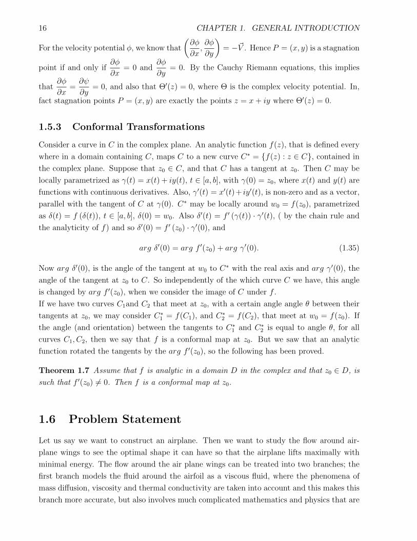
16 CHAPTER 1. GENERAL INTRODUCTION
For the velocity potential φ, we know that
(∂φ
∂x,∂φ
∂y
)= −~V . Hence P = (x, y) is a stagnation
point if and only if∂φ
∂x= 0 and
∂φ
∂y= 0. By the Cauchy Riemann equations, this implies
that∂φ
∂x=∂ψ
∂y= 0, and also that Θ′(z) = 0, where Θ is the complex velocity potential. In,
fact stagnation points P = (x, y) are exactly the points z = x+ iy where Θ′(z) = 0.
1.5.3 Conformal Transformations
Consider a curve in C in the complex plane. An analytic function f(z), that is defined every
where in a domain containing C, maps C to a new curve C∗ = {f(z) : z ∈ C}, contained in
the complex plane. Suppose that z0 ∈ C, and that C has a tangent at z0. Then C may be
locally parametrized as γ(t) = x(t) + iy(t), t ∈ [a, b], with γ(0) = z0, where x(t) and y(t) are
functions with continuous derivatives. Also, γ′(t) = x′(t)+ iy′(t), is non-zero and as a vector,
parallel with the tangent of C at γ(0). C∗ may be locally around w0 = f(z0), parametrized
as δ(t) = f (δ(t)), t ∈ [a, b], δ(0) = w0. Also δ′(t) = f ′ (γ(t)) · γ′(t), ( by the chain rule and
the analyticity of f) and so δ′(0) = f ′ (z0) · γ′(0), and
arg δ′(0) = arg f ′(z0) + arg γ′(0). (1.35)
Now arg δ′(0), is the angle of the tangent at w0 to C∗ with the real axis and arg γ′(0), the
angle of the tangent at z0 to C. So independently of the which curve C we have, this angle
is changed by arg f ′(z0), when we consider the image of C under f .
If we have two curves C1and C2 that meet at z0, with a certain angle angle θ between their
tangents at z0, we may consider C∗1 = f(C1), and C∗2 = f(C2), that meet at w0 = f(z0). If
the angle (and orientation) between the tangents to C∗1 and C∗2 is equal to angle θ, for all
curves C1, C2, then we say that f is a conformal map at z0. But we saw that an analytic
function rotated the tangents by the arg f ′(z0), so the following has been proved.
Theorem 1.7 Assume that f is analytic in a domain D in the complex and that z0 ∈ D, is
such that f ′(z0) 6= 0. Then f is a conformal map at z0.
1.6 Problem Statement
Let us say we want to construct an airplane. Then we want to study the flow around air-
plane wings to see the optimal shape it can have so that the airplane lifts maximally with
minimal energy. The flow around the air plane wings can be treated into two branches; the
first branch models the fluid around the airfoil as a viscous fluid, where the phenomena of
mass diffusion, viscosity and thermal conductivity are taken into account and this makes this
branch more accurate, but also involves much complicated mathematics and physics that are

1.6. PROBLEM STATEMENT 17
Figure 1.11: A conformal transformation [3]
beyond the scope of this thesis.
Instead, we consider the second branch, that models the fluid flow around the airfoil
as an ideal fluid flow. Ideal fluid flows refer to fluid motions that are steady, inviscid,
incompressible, and irrotational [10]. However such flows do not exist in reality, but there are
many practical aerodynamic flows where the influence of the transport phenomena is small,
and it can be modeled as being inviscid. Considering the fluid flow around the airfoil as
inviscid and incompressible still allows for an accurate model provided certain conditions are
met [1]. One of these conditions is that the airplane wing must be moving through the fluid
at subsonic speeds; this is very crucial because at speeds approaching the speed of sound,
shock waves occur in which the fluid flow no longer becomes continuous, and the perfect
fluid idealization breaks down. In particular, we will build our models for airfoils moving
through flows regions where the compressibility effects in the fluid flow can be negligible
(Mach number between 0.0 and 0.4) [13]. Another assumption is that the flow around the
Figure 1.12: Inviscid flow over an airfoil with the Kutta condition satisfied. The flow meets
smoothly at the trailing edge. [4]
airplane wing satisfies the Kutta Condition (see figure 1.12). The Kutta condition is that the
fluid flowing over the upper and lower surfaces of the airfoil meets smoothly at the trailing
edge of the airfoil and explains how an inviscid fluid can generate lift. Thus, the Kutta
condition accounts for the friction at the boundary of an airfoil that is essential for lift to
18 CHAPTER 1. GENERAL INTRODUCTION
be generated under other additional constraints on the flow around an airfoil [1]. With
reference to subsection 1.3.2 a fluid flow is said to be an incompressible flow if its density ρ is
constant, in contrast, it is called compressible when ρ varies. The fluid flow where the density
is precisely constant does not exist in nature, but analogous to our discussions of nonviscous
flow, there are many aerodynamic problems which can be modeled as incompressible flows
without loss of accuracy [10]. In this case the equation of continuity (1.7) reduces to (1.8).
Furthermore, the absence of frictional shear forces acting on elements of an inviscid fluid
causes the motion of the fluid to be purely translational, allowing the flow over an airfoil to
be modeled as irrotational [1]. Again this irrotationality property of the fluid motion results
in equation (1.13) due to the fact that the curl of the velocity vanishes. Since the motion
is irrotational, its velocity field ~V can be expressed as the gradient of a scalar function φ in
the sense that ~V = ∇φ. We call φ the velocity potential, and the flows that result from a
velocity potential are known as potential flows. We saw in (1.28) that φ satisfies the Laplace
equation
∇2φ = 0,
and solutions to this equation are referred to as harmonic functions. Since Laplace’s equa-
tion is a linear homogeneous second order partial differential equation, the sum of particular
solutions to the differential equation is also a solution [10]. This means that we can study
complicated stream functions that one built up from simpler ones, a technique which the rest
of the thesis will give an example of.
Due to the fact the air plane wings have complicated geometries; it is difficult to directly
solve for the fluid flow around them using Laplace equation and potential flow theory. To
do this in a more efficient way; we define a complex potential function in the z− plane as
defined in theorem 1.5. When the complex potential function is transformed using conformal
mapping techniques, the stream function and potential remained unchanged. In this thesis we
will first solve the flow around a cylinder in the z plane, and then transform this solution to an
airfoil in the w plane using a specific conformal mapping function. We will also implement the
Joukowsky transformation to compute the fluid flow and lift around the Joukowsky airfoils
using some computer algebra systems.

1.7. OBJECTIVES 19
1.7 Objectives
We will first go through the theories behind modeling of a two- dimensional fluid flow and
summarize some theories of complex analysis and that of conformal mappings. These will
comprise the introductory part of the thesis. We will then construct the fluid flow in a com-
plicated domain from known flows in a simpler domain, using conformal mappings.
The Specific Objectives are:
1. To study and understand the basic ideas and concepts of conformal mapping.
2. Describe the mathematical model used to model the inviscid incompressible fluid flow
around the airplane wing.
3. Apply the theories of conformal mapping using Joukowsky transformation to link the
solution for flow around a cylinder to the solution for flow around the air plane wing.
4. Attempt to implement this conformal mapping transformation to compute the fluid
flow and lift around some airplane wings.
1.7.1 Scope of the Study
The scope of the study will be limited to the specific objectives listed above; in particular to
exhibit the most basic and simple examples of the use of conformal mapping to compute the
fluid flow.
1.7.2 Significance of the Study
To introduce in a readable way to mathematics and physics students one of the more fasci-
nating applications of complex function theory to engineering.
1.8 Outline
This thesis is organized as follows: The first part of the thesis consists of the introduction.
In this part, a lot of definitions of the important terms were provided. It also includes the
description of several key concepts that play an important role in this dissertation including
the concepts of fluids dynamics, the concept of circulation, the concept of stream function
and velocity potential, the concepts of complex analysis and some concepts of conformal
transformation. These concepts explain how the conformal mapping technique is a viable
option to transform the potential flows.
The second part consists of the literature about the mathematical model used to model the
lifting fluid flow around the circular cylinder and its implementation in MATLAB.
20 CHAPTER 1. GENERAL INTRODUCTION
The third part will be about the use of a conformal mapping technique to transform the
circular cylinder into another shape such as an ellipse or an airfoil. In this part the complex
potential will be described to show how the lift and circulation remained unchanged when
the complex potential is subjected to conformal transformation.
After discussing this, the streamlines around the circular cylinder and around the correspond-
ing airfoil will be computed using MATLAB software. Again , the lift force will be calculated
using the Kutta-Joukowsky formula. Finally, the lift coefficient as function of the angle of
attack for the Joukowsky airfoil 12% and the NACA 0012 airfoil will be compared and the
results will be summarized and some ideas for further studies will be suggested.

Chapter 2
Literature Review
2.1 Modeling the Fluid around an Airplane Wing
In this section, we will review some elementary incompressible flows which will be superim-
posed to get more complex incompressible flows to be able to model the fluid flow around an
airfoil by simply solving the lifting flow around a cylinder in the plane.
2.1.1 Uniform Flow
We consider the uniform flow as our first elementary incompressible flow. Consider a flow
with a free-stream velocity V∞ that is oriented in the positive x direction as illustrated in
figure 2.1 since the uniform flow is irrotational, its velocity ~V can be expressed as ~V = ∇φ,
with the potential function φ. It then follows that
~V = ∇φ⇔
∂φ
∂x= u = V∞
∂φ
∂y= v = 0.
(2.1)
The potential function φ is found by integration with respect to x first and then to y and
comparing the results to get φ = V∞x+ const. The constant can be removed from φ because
the velocity if obtained by differentiation, thus φ = V∞x. Considering also the stream
function we have ∂ψ
∂y= u = V∞
∂ψ
∂x= −v = 0.
(2.2)
Similarly, by integration with respect to x first and then to y and comparing the results gives
ψ = V∞y which is the stream function of the uniform flow oriented in the positive x direction.
In polar coordinates the potential function and the stream functions are written as follows:
φ = V∞r cosφ, where x = r cos θ and ψ = V∞r sin θ. From the equations (2.1) and (2.2), it
can be shown that the uniform flow satisfies the Laplace equation and the stream lines (for
21

22 CHAPTER 2. LITERATURE REVIEW
y = const) and the equipotential curves (for x = const ) are perpendicular. More details
about the uniform flow can be found in [5, 23]
Figure 2.1: Uniform Flow (on the left) [10] and Computed uniform flow in MATLAB with
streamlines (blue) and equipotential curves (red) on the right
2.1.2 Source and Sink Flow
Consider an incompressible flow in two dimensions where all the streamlines are the straight
lines either converging or diverging from the center O as shown in figure 2.3. If all the
Figure 2.2: Source flow [16]
streamlines are converging to the center, the flow is called the sink flow. In contrast, when
the stream lines are emerging from the central point, the flow is referred to as a source
flow. The coordinate system for the figure 2.3 is a cylindrical coordinate system with the
z - axis perpendicular to the page. It is not difficult to show that the source flow is an
incompressible flow (∇ ·V = 0), at every point except the origin, where (∇ ·V =∞), and as
well as irrotational flow at every point. In the sink flow, the stream lines are directed towards
the origin and are still radial lines from the common origin along which the flow velocity is
assumed to vary inversely proportional to the distance from the central point. It means
that the radial component of the resultant Vr =c
r, where c is a constant and the tangential

2.1. MODELING THE FLUID AROUND AN AIRPLANE WING 23
Figure 2.3: Sink flow [4]
Figure 2.4: Source Flow with streamlines (blue) and velocity potential in red (on left) and
Sink Flow streamlines (blue) and equipotential curves in yellow (on right) both computed in
MATLAB.
Figure 2.5: Volume flow rate from a line source [10]
component is Vθ = 0. Considering the mass flow across the surface of the cylinder of r radius
and height l as illustrated in figure 2.5, it is not difficult to see that the elemental mass flow
across the surface element dS is equal to ρV · dS = ρVr(rdθ)(l). Since Vr is the same at any
location for the fixed radius r, the total mass flow across the surface of the cylinder is
m =
∫ 2π
0
ρVr(rdθ)l = ρrlVr
∫ 2π
0
dθ = 2πrlρVr. (2.3)

24 CHAPTER 2. LITERATURE REVIEW
Because ρ is defined as the mass per unit volume and m the mass per second, then we will
define the volume flow per second v as v = mρ
. And then, from the equation (2.3), we get
v =m
ρ= 2πrlVr. (2.4)
Let Λ be the rate of change of the volume ( volume flow from the source) per unit length
(Λ =v
l) called the source strength. Using the above boundary conditions it can be shown
that the potential and the stream functions are φ =Λ
2πlnr, and ψ =
Λ
2πθ, respectively with
r the distance from the origin [10, 24]. If Λ has a positive value, the flow is a source flow
and it is a sink flow whenever Λ has a negative value.
2.1.3 A Combination of a Uniform Flow with a Source and Sink
Flow
Consider a uniform stream with the free stream velocity V∞ oriented from left to right.
Superimpose it to a source flow of strength Λ located at the origin in polar coordinates as
shown in figure 2.6. The stream function for the resulting flow is simply found by addition
Figure 2.6: A combination (superposition) of a uniform flow and a source flow generates a
flow over a semi-infinite body [10]
Figure 2.7: A combination (superposition) of a uniform flow and a source flow generates a
flow over a semi-infinite body with streamlines (blue) and equipotential curves (red).

2.1. MODELING THE FLUID AROUND AN AIRPLANE WING 25
of the stream functions of the two flows. It means
ψ = V∞r sin θ +Λ
2πθ [5]. (2.5)
This equation satisfies the Laplace equation as it is the sum of the functions where each func-
tion satisfies the Laplace equation alone. From this, it is reasonable to say that the equation
(2.5) describes an irrotational, incompressible flow. The streamlines of the superimposed
flow are found by setting ψ = V∞r sin θ +Λ
2πθ = const. The velocity field can be found by
differentiating equation 2.5 as follows:
Vr =1
r
∂ψ
∂θ= V∞ cos θ +
Λ
2πr. (2.6)
and
Vθ = −∂ψ∂r
= −V∞ sin θ. (2.7)
The stagnation points in the flow can be found by equating the equations 2.6 and 2.7 equal
to zero: This is V∞ cos θ +Λ
2πr= 0, and −V∞ sin θ = 0. The coordinates of the stagnation
points are obtained by solving for r, and θ thus (r, θ) =
(Λ
2πV∞, π
), and is labeled as point
B in figure 2.6. The equation of the stream function that goes through the stagnation point
is obtained by substituting its coordinates into this equation ψ = V∞r sin θ+Λ
2πθ = const, to
get: ψ = V∞Λ
2πV∞sin π = const ⇔ ψ =
Λ
2= const, hence the curve ABC in the schematic
2.6 is the streamline described by ψ =Λ
2[10].
2.1.4 Doublet flow
A doublet flow is a particular, degenerate case a source -sink combination that leads to a
singularity. This kind of flow is often used in the theory of incompressible flow.The stream
function for a doublet flow is
ψ = − κ
2π
sin θ
r. (2.8)
Similarly, it can be shown that velocity potential for a doublet flow is given by
φ =κ
2π
cos θ
r. (2.9)
We find the streamlines of a doublet flow by setting ψ = − κ
2π
sin θ
r= const = c. And using
the fact that r = d sin θ, it can be shown that the streamlines are a family of circles with
diameterκ
2πc, as shown in figure 2.8.

26 CHAPTER 2. LITERATURE REVIEW
Figure 2.8: (Left) Doublet flow with strength κ [16],Computed Doublet flow (right) in
MATLAB with strength κ = 0.05 and streamlines (blue) and equipotential curves (red).
2.1.5 Superposition of a Uniform Flow and a Doublet Flow
The superposition of the uniform flow and the doublet flow yields the flow over a circular
cylinder. A circular cylinder is among the most elementary geometrical shapes available and
the study of the flow around it has been classically an interesting problem in aerodynamics.
Consider a superposition of a uniform flow with a freestream velocity V∞ and a doublet of
strength κ as illustrated in figure 2.9. The stream function of the superimposed flow is given
Figure 2.9: The synthesis non-lifting flow over a cylinder. [10]
.
Figure 2.10: Computed nonlifting flow in MATLAB as superposition of a uniform and a
doublet flows with streamlines (blue) and equipotential curves (red).

2.1. MODELING THE FLUID AROUND AN AIRPLANE WING 27
by
ψ = V∞r sin θ − κ
2π
sin θ
r, (2.10)
ψ = V∞r sin θ
(1− κ
2πV∞r2
),
ψ = (V∞r sin θ)
(1− R2
r2
), where R2 ≡ κ/2πV∞. (2.11)
The equation (2.11) shows the stream function of the flow over a circular cylinder of radius
R =
√κ
2πV∞. (2.12)
The velocity field is:
Vr =1
r
∂ψ
∂θ=
1
r(V∞ cos θ)
(1− R2
r2
)=
1
r
(1− R2
r2
)V∞ cos θ. (2.13)
and
Vθ = −∂ψ∂r
= −[(V∞ sin θ)
2R2
r2+
(1− R2
r2
)V∞ sin θ
]= −
(1 +
R2
r2
)V∞ sin θ. (2.14)
From the equations (2.13) and (2.14) , we obtain the stagnation points by solving simulta-
neously the following equations
−(
1 +R2
r2
)V∞ sin θ = 0;
(1− R2
r2
)V∞ cos θ = 0;
and solving for r and θ we get the following stagnation points: (r, θ) = (R, 0) or (r, θ) =
(R, π), denoted A and B in figure 2.9. The flow around a circular cylinder is symmetrical
about both the horizontal axis and vertical axis through the center of the cylinder as clearly
illustrated by the streamline sketched in figure 2.9. Therefore, the pressure gradient is also
symmetrical about both axes meaning that the pressure distribution over the bottom of the
cylinder is exactly balanced by the pressure distribution over the top of the cylinder and
consequently the net lift cannot be generated over the cylinder. Similarly, there is
no net drag, because the pressure distribution over the front of the cylinder is also exactly
balanced with that over the back of the cylinder. That is why the vortex flow is needed to
model the lifting over the circular cylinder [1].
28 CHAPTER 2. LITERATURE REVIEW
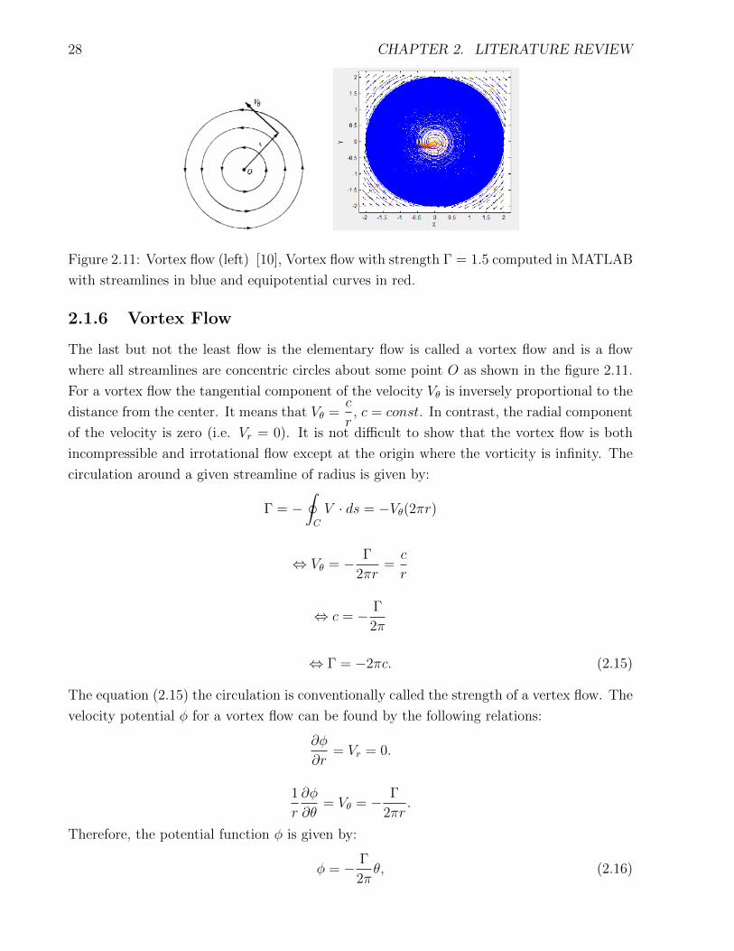
Figure 2.11: Vortex flow (left) [10], Vortex flow with strength Γ = 1.5 computed in MATLAB
with streamlines in blue and equipotential curves in red.
2.1.6 Vortex Flow
The last but not the least flow is the elementary flow is called a vortex flow and is a flow
where all streamlines are concentric circles about some point O as shown in the figure 2.11.
For a vortex flow the tangential component of the velocity Vθ is inversely proportional to the
distance from the center. It means that Vθ =c
r, c = const. In contrast, the radial component
of the velocity is zero (i.e. Vr = 0). It is not difficult to show that the vortex flow is both
incompressible and irrotational flow except at the origin where the vorticity is infinity. The
circulation around a given streamline of radius is given by:
Γ = −∮C
V · ds = −Vθ(2πr)
⇔ Vθ = − Γ
2πr=c
r
⇔ c = − Γ
2π
⇔ Γ = −2πc. (2.15)
The equation (2.15) the circulation is conventionally called the strength of a vertex flow. The
velocity potential φ for a vortex flow can be found by the following relations:
∂φ
∂r= Vr = 0.
1
r
∂φ
∂θ= Vθ = − Γ
2πr.
Therefore, the potential function φ is given by:
φ = − Γ
2πθ, (2.16)

2.1. MODELING THE FLUID AROUND AN AIRPLANE WING 29
and is found by integration of the above equations. Again, we find the stream function ψ in
the same fashion, and it is
ψ =Γ
2πln r. (2.17)
2.1.7 Lifting Flow over a Cylinder
The lifting flow over a cylinder is a combination of a non-lifting flow discussed in section 2.1.5
and a vortex flow of strength Γ as shown in the figure 2.12. The stream function and the
Figure 2.12: The synthesis flow of a lifting flow over a cylinder [10]
.
potential function of the lifting flow over a cylinder are obtained by addition of the stream
function and the potential function of the non-lifting flow and those of the vortex flow and
are written below:
ψ = V∞r sin θ − κ
2π
sin θ
r+
Γ
2πln r,
⇔ ψ = V∞r sin θ
(1− R2
r2
)+
Γ
2πln r. (2.18)
φ = V∞r cos θ − Γ
2πθ +
κ
2π
cos θ
r. (2.19)
Note that the streamlines for this flow are no longer symmetric about the horizontal axis
through the central point O, however, the streamlines are symmetrical about the vertical
axis through O and hence they will be no drag. Also note that the circulation is finite and
is equal to Γ because the vortex of strength Γ has been added to the flow. The velocity
components are found by differentiating ψ . It means that
Vr =
(1− R2
r2
)V∞ cos θ. (2.20)
Vθ =
(1− R2
r2
)V∞ sin θ − Γ
2πr[5]. (2.21)
30 CHAPTER 2. LITERATURE REVIEW
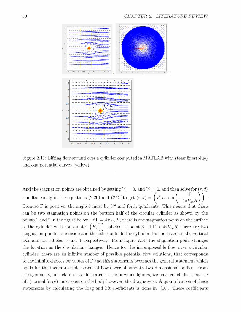
Figure 2.13: Lifting flow around over a cylinder computed in MATLAB with steamlines(blue)
and equipotential curves (yellow).
.
And the stagnation points are obtained by setting Vr = 0, and Vθ = 0, and then solve for (r, θ)
simultaneously in the equations (2.20) and (2.21)to get (r, θ) =
(R, arcsin
(− Γ
4πV∞R
)).
Because Γ is positive, the angle θ must be 3rd and forth quadrants. This means that there
can be two stagnation points on the bottom half of the circular cylinder as shown by the
points 1 and 2 in the figure below. If Γ = 4πV∞R, there is one stagnation point on the surface
of the cylinder with coordinates(R,
π
2
), labeled as point 3. If Γ > 4πV∞R, there are two
stagnation points, one inside and the other outside the cylinder, but both are on the vertical
axis and are labeled 5 and 4, respectively. From figure 2.14, the stagnation point changes
the location as the circulation changes. Hence for the incompressible flow over a circular
cylinder, there are an infinite number of possible potential flow solutions, that corresponds
to the infinite choices for values of Γ and this statements becomes the general statement which
holds for the incompressible potential flows over all smooth two dimensional bodies. From
the symmetry, or lack of it as illustrated in the previous figures, we have concluded that the
lift (normal force) must exist on the body however, the drag is zero. A quantification of these
statements by calculating the drag and lift coefficients is done in [10]. These coefficients

2.1. MODELING THE FLUID AROUND AN AIRPLANE WING 31
Figure 2.14: Stagnation points on a lifting flow over a circular cylinder. [10]
.
are defined as dimensionless quantities(numbers) that areodynamicists use to model all the
complex dependencies of shape, inclination and some flow conditions on either airplane lift
or drag and as a result the lift coefficient for inviscid , incompressible fluid is
cl =Γ
RV∞. (2.22)
and it relates the lift generated by an airfoil, the dynamic pressure on the fluid flow around
the airfoil and the area of the airfoil. The drag coefficient is
cd = 0, (2.23)
regardless on whether or not the flow has the circulation about the cylinder. The proof is
left for the leader and can be found in [10], section 3.15.
2.1.8 Lift and Drag around two Dimensional Shapes
No matter what the cross section shape of any cylindrical body, one can relate the ideal
Lift and Drag force to the complex potential. In practice we will concentrate on cylinders
transformed into an airfoil shape. Any bluff shape would have awake of finite thickness, and
this would invalidate the theory. The entire flow must be an ideal flow defined in section
1.6 for this theory to apply. Boundary layers and wakes must be vanishingly thin. Consider
an incompressible flow over an airfoil as shown in figure 2.15 and let A be any curve in the
fluid flow enclosing the airfoil, then the circulation if given by Γ ≡∮AV · ds, where V is
the velocity field around the airfoil and the airfoil is generating a lift. It will turn out that
the drag force is always zero; Fd = 0, and that the lift force is directly proportional to the
circulation constant Γ. The exact relation for the lift force is
L = ρ∞V∞Γ. [16] (2.24)
Where ρ∞ is the fluid density and V∞ is the fluid velocity far upstream of the airfoil and Γ
is the circulation defined in figure 2.15. This is the Kutta-Joukowsky theorem. For the
32 CHAPTER 2. LITERATURE REVIEW
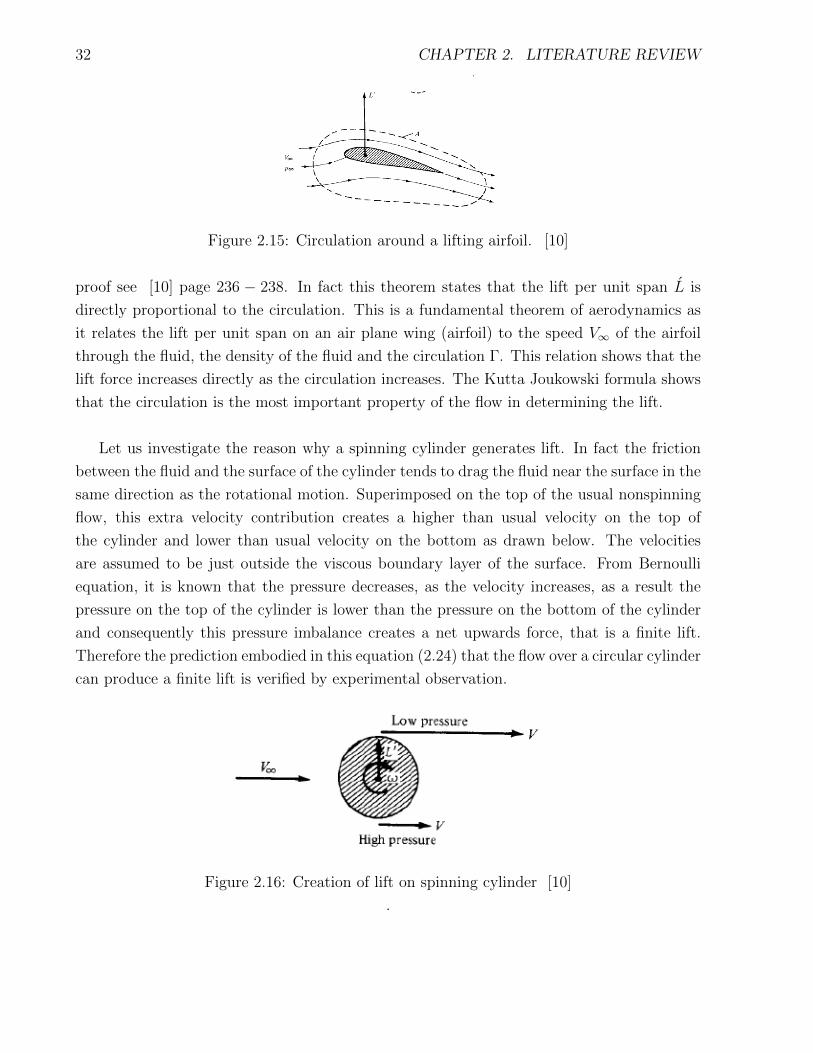
Figure 2.15: Circulation around a lifting airfoil. [10]
proof see [10] page 236 − 238. In fact this theorem states that the lift per unit span L is
directly proportional to the circulation. This is a fundamental theorem of aerodynamics as
it relates the lift per unit span on an air plane wing (airfoil) to the speed V∞ of the airfoil
through the fluid, the density of the fluid and the circulation Γ. This relation shows that the
lift force increases directly as the circulation increases. The Kutta Joukowski formula shows
that the circulation is the most important property of the flow in determining the lift.
Let us investigate the reason why a spinning cylinder generates lift. In fact the friction
between the fluid and the surface of the cylinder tends to drag the fluid near the surface in the
same direction as the rotational motion. Superimposed on the top of the usual nonspinning
flow, this extra velocity contribution creates a higher than usual velocity on the top of
the cylinder and lower than usual velocity on the bottom as drawn below. The velocities
are assumed to be just outside the viscous boundary layer of the surface. From Bernoulli
equation, it is known that the pressure decreases, as the velocity increases, as a result the
pressure on the top of the cylinder is lower than the pressure on the bottom of the cylinder
and consequently this pressure imbalance creates a net upwards force, that is a finite lift.
Therefore the prediction embodied in this equation (2.24) that the flow over a circular cylinder
can produce a finite lift is verified by experimental observation.
Figure 2.16: Creation of lift on spinning cylinder [10]
.

Chapter 3
Methodology
3.1 The Conformal Mapping Technique
As described in subsection 1.2.1 the airplane wings have complicated geometry, it is then diffi-
cult to directly solve for the fluid flow around the airfoils using Laplace equation and potential
flow theory. To simplify the problem, the conformal mapping technique is used to extend the
application of potential flow theory to practical aerodynamics [1]. The main advantage of
conformal mapping in solving the fluid flow problems is that solutions of the Laplace equation
for φ(x, y) and ψ(x, y), remain solutions when subjected to conformal transformation. Let
us consider a conformal mapping from z = x + iy− plane to a w = f(z) = u + iv− plane
as defined in subsection 1.5.3. And in section 1.5.1, we have proved that the z−plane is
conformally mapped to the w− plane, in which the Laplace equation is still satisfied for each
φ(x, y) and ψ(x, y). We can now solve for them in the transformed w = f(z)− plane, and
then compute the solution by the inverse transformation to the original z− plane because
the transformed boundaries in the u, v− plane take a simpler form. In summary, the solution
of a flow problem found by conformal mapping consists of the following steps:
1. Map the given flow domain D ∈ C onto a geometrically simpler flow domain D′ ∈ Cusing conformal transformation, here boundary conditions φ and ψ remain the same
for the transformed boundaries.
2. Solve the Laplace equation of either φ and or ψ in the transformed domain.
3. Use the inverse transformation to derive φ = φ(x, y), ψ = ψ(x, y). Sometimes a
sequence of conformal mappings is needed before a solution for φ and or ψ can be
found [12].
For instance, let us consider the z = x+ iy− plane of a uniform fluid flow horizontal stream-
lines given by φ = iy, and equipotential curves given by ψ = x. In figure 3.1, a conformal
mapping given by f(z) =√z, is used to transform this complex plane z into a new complex
33

34 CHAPTER 3. METHODOLOGY
Figure 3.1: A conformal mapping of a uniform flow with the conformal function w(z) =√z. The vertical lines in (a) represent equipotential curves, the horizontal lines represent
streamlines. In (b), the conformal map maintains the right angle relationship between the
streamlines and equipotential curves [1]
.
plane w. It is clear that this transformation has changed the relative shape of the streamlines
and equipotential curves, but the set of curves remains perpendicular. This angle preserving
feature is the essential component of conformal mapping. Since the relative orientation of the
streamlines and potential curves remains unchanged, any harmonic function in the z plane,
is also harmonic in the transformed w plane [12]. In the next section, we will show how the
flow around an airfoil shape can be constructed by first solving for the flow around a cylinder
in the z plane, and then transforming this solution to an airfoil in the w plane using a specific
conformal mapping function.
3.2 Mapping from a Circular Cylinder to an Airfoil
with the Joukowsky Transformation
In section 2.1.7 we have seen that the two dimensional incompressible, inviscid, irrotational
flow around a cylinder is generated by the superposition of three elementary flows, namely
a uniform flow, source-sink flow and a vortex flow. The stream function ψ of such a flow is
given by the equation (2.18). The flow around a circular cylinder can be mapped into the
flow about another body by using conformal mapping with the complex potential preserved.
The most known conformal transformation is the Joukowsky transformation given by:
w = f(z) = z +λ2
z, (3.1)
where w is the function in the transformed plane and λ is the parameter of the transformation
that determines the resulting shape of the transformed function. Let z = x+ iy = r(cos θ +
i sin θ) = reiθ, this is a circle of radius r and the center at the origin in the z− plane [21].

3.2. MAPPING FROMACIRCULAR CYLINDER TOANAIRFOILWITH THE JOUKOWSKY TRANSFORMATION35
And this implies that
w = f(z) = z +λ2
z= reiθ +
λ2
re−iθ (3.2)
⇔
w = r cos θ + ir sin θ +λ2
r(cos θ − i sin θ)
⇔
w = r cos θ + ir sin θ +λ2
r(cos θ − i sin θ)
⇔
w = r cos θ +λ2
rcos θ + ir sin θ − iλ
2
r(sin θ)
⇔
w = (r +λ2
r) cos θ + i(r − λ2
r) sin θ
⇔
w = a cos θ + ib sin θ, (3.3)
where a = r +λ2
r, b = a = r − λ2
r, and also w = u+ iv,
⇒
u = a cos θ
v = b sin θ,
⇒
cos θ =u
asin θ =
v
b.
But cos2 θ + sin2 θ = 1, ⇒(ua
)2
+(vb
)2
= 1 ⇔ 1
a2u2 +
1
b2v2 = 1. If we set the parameter
λ = r, then a = r+r2
r, and b = r− r2
r, and this implies that a = 2r, b = 0, and from this it
can be seen that the circle in the z−plane is transformed into a flat plate of length 4r in the
w−plane. It means that the points of the circle in z−plane occupy the strip −2r ≤ u ≤ 2r,
in the w−plane. For λ ≥ r, the circle in the z− plane is transformed into an ellipse in the
w− plane; this is (u
r + λ2
r
)2
+
(v
r − λ2
r
)2
= 1, (3.4)
⇒ u2
r2(1 + λ2/r3)2+
v2
r2(1− λ2/r3)2= 1, (3.5)
which is an equation of ellipse centered at the origin with the semi major axis a = r(1+λ2/r3),
and the minor axis b = r(1− λ2/r3). Now the implementation of this in MATLAB is shown
below:

36 CHAPTER 3. METHODOLOGY
Figure 3.2: A circular cylinder centered at the origin in the z−plane with radius r = 1,
and λ = 1 (1). The corresponding flat plate of length 4 in the w−plane transformed using
Joukowsky transformation (2). This is implemented in MATLAB.
Figure 3.3: (3) A circular cylinder centered at the origin in the z−plane with radius r = 1,
and λ > 1, and (4) The flow around the corresponding ellipse in the w−plane transformed
using Joukowsky transformation.
Nevertheless, none of the shapes 3.2 and 3.3 look like an airfoil. The airfoil shape is
found by considering a circle in the z−plane which is not centered at the origin. The circle
in the z− plane is slightly offset using the following parameter transformation: λ = r − |t|,with t the coordinate of the center of the circle in the z−plane. In this case the image
in the w− plane look like the shape of an uncambered airfoil which is symmetric about the
x−axis, as illustrated in figure 3.4. The x coordinate of the circle consequently determines the
thickness distribution of the transformed airfoil. When the center of the circle in the z−plane
is again offset on the y axis, we get an unsymmetrical, cambered airfoil as shown in figure
3.5. And this shows that the y coordinate of the center of circle determines the curvature of
the transformed airfoil in the w−plane. The Joukowsky transformation creates the airfoils

3.2. MAPPING FROMACIRCULAR CYLINDER TOANAIRFOILWITH THE JOUKOWSKY TRANSFORMATION37
shapes known as Joukowsky airfoils. The leading and trailing edges of the transformed airfoil
in the w plane correspond to the x intercepts of the circle in the z− plane [15].
Figure 3.4: (a) A circular cylinder centered at (−0.105, 0), (the center is offset on the x axis)
in the z−plane with radius r = 1.205, and λ = 1 − |t|. (b) The corresponding symmetric
uncambered airfoil in w−plane obtained using Joukowsky transformation of the cylinder.
Figure 3.5: (c) A circular cylinder centered at (0.3, 0.12), (the center is offset on the x and
y axes) in the z−plane with radius r = 1.202, and λ = 1 − |t|. (d) The corresponding (non
symmetric) cambered airfoil in w−plane obtained using Joukowsky transformation of the
cylinder.
38 CHAPTER 3. METHODOLOGY
Figure 3.5 (b) also shows that the Joukowsky airfoil has a cusp at the trailing edge, which
is a mathematical property that is not present in real airfoil shapes [16]. Besides to above
transformation, the flow around the circular cylinder can be transformed by the conformal
mapping functions. This is done by expressing the velocity potential φ and stream function
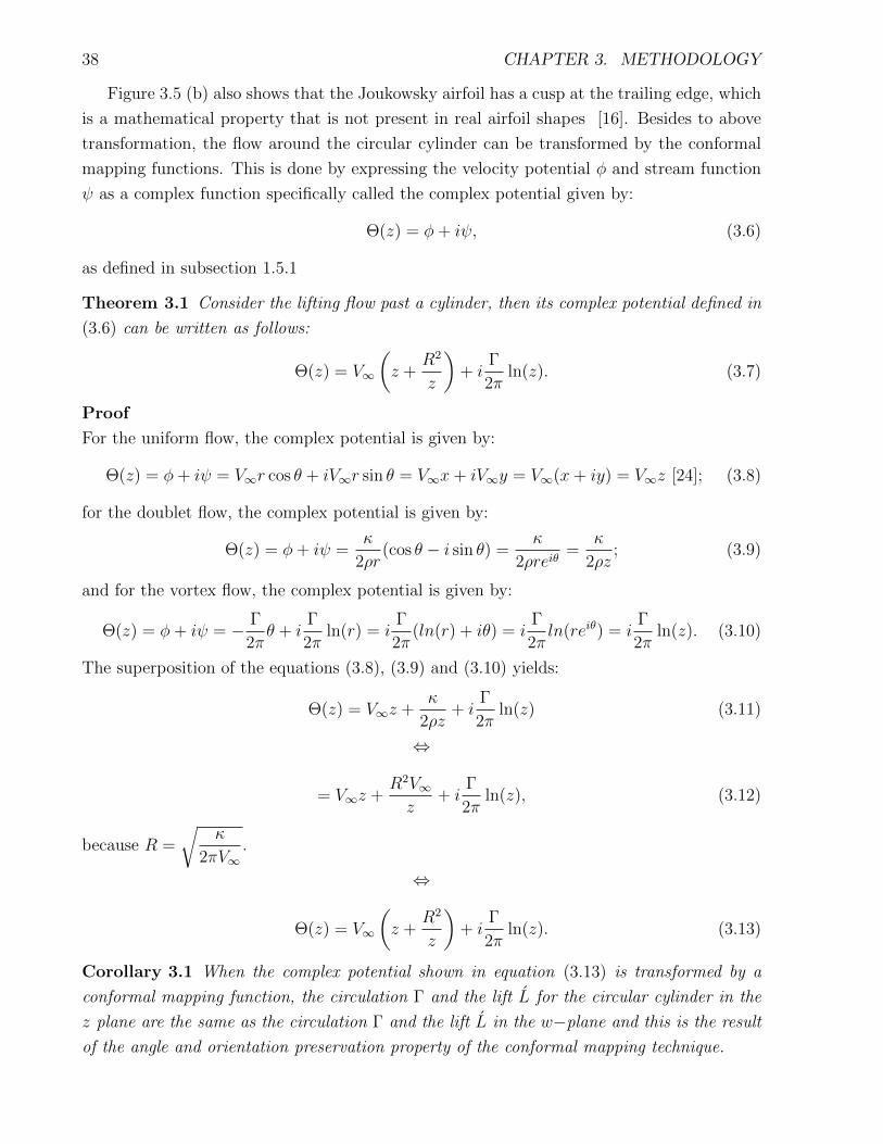
ψ as a complex function specifically called the complex potential given by:
Θ(z) = φ+ iψ, (3.6)
as defined in subsection 1.5.1
Theorem 3.1 Consider the lifting flow past a cylinder, then its complex potential defined in
(3.6) can be written as follows:
Θ(z) = V∞
(z +
R2
z
)+ i
Γ
2πln(z). (3.7)
Proof
For the uniform flow, the complex potential is given by:
Θ(z) = φ+ iψ = V∞r cos θ + iV∞r sin θ = V∞x+ iV∞y = V∞(x+ iy) = V∞z [24]; (3.8)
for the doublet flow, the complex potential is given by:
Θ(z) = φ+ iψ =κ
2ρr(cos θ − i sin θ) =
κ
2ρreiθ=
κ
2ρz; (3.9)
and for the vortex flow, the complex potential is given by:
Θ(z) = φ+ iψ = − Γ
2πθ + i
Γ
2πln(r) = i
Γ
2π(ln(r) + iθ) = i
Γ
2πln(reiθ) = i
Γ
2πln(z). (3.10)
The superposition of the equations (3.8), (3.9) and (3.10) yields:
Θ(z) = V∞z +κ
2ρz+ i
Γ
2πln(z) (3.11)
⇔
= V∞z +R2V∞z
+ iΓ
2πln(z), (3.12)
because R =
√κ
2πV∞.
⇔
Θ(z) = V∞
(z +
R2
z
)+ i
Γ
2πln(z). (3.13)
Corollary 3.1 When the complex potential shown in equation (3.13) is transformed by a
conformal mapping function, the circulation Γ and the lift L for the circular cylinder in the
z plane are the same as the circulation Γ and the lift L in the w−plane and this is the result
of the angle and orientation preservation property of the conformal mapping technique.

Chapter 4
Results and Analysis
This chapter focus on computations aspects involved in solving our problem. MATLAB
software is used to visualize how the lifting flow around a circular cylinder can be transformed
into the flow around the Joukowsky airfoils and then calculate lift.
4.1 Computing the Streamlines around an Airfoil and
Lift calculation
When a Joukowsky transformation is applied to an offset circular cylinder, one can get the
Joukowsky airfoils by the use for instance of mathlab program. The contour plot of the
imaginary part of the complex potential of the equation (3.13) gives the flow around the
airfoil. The lift force is calculated using the formula in equation(2.24)
L = V∞ρ∞Γ,
where
Γ =2rV∞ sinα
2π. (4.1)
and the angle α that we have in the equation (4.1) was measured in radians and when
converted into degrees amounts toαπ
180. At zero angle of attack, there is no lift generated
on the cylinder and on the airfoil because the fluid flow is symmetric. This is due to the
fact that there is a symmetric distribution of the streamlines about the x axis on both the
circular cylinder in the z plane and the airfoil in the w plane. Again, looking on the airfoil,
it is clear that the streamlines meet at the trailing edge, and therefore the Kutta condition
is satisfied. In this experience, we are going to compute the streamlines around the circular
cylinder and the corresponding airfoil at different values of angle of attack. In figure 4.2, the
calculated lift force is 6.5552 N/m at α = 4, in figure 4.3, the lift force found is 13.0785 N/m
at α = 8, in figure 4.4, we have got the lift force equal to 19.5381 N/m at α = 12, and finally
we have got 24.322 N/m as the lift force at α = 15.
39

40 CHAPTER 4. RESULTS AND ANALYSIS
Figure 4.1: The streamlines around circular cylinder plot computed in the z plane and the
corresponding symmetric Joukowsky airfoil. The plot was generated with V∞ = 200m/s, α =
0, and ρ = 1.225 kg/m3. The cylinder parameters used: x = −0.105 m, y = 0 m, r =
1.205 m.
Figure 4.2: The streamlines around circular cylinder plot computed in the z plane and the
corresponding symmetric Joukowsky airfoil. The plot was generated with V∞ = 200m/s, α =
4, and ρ = 1.225 kg/m3. The cylinder parameters used: x = −0.105 m, y = 0 m, r =
1.205 m.
In figure 4.6, we generated a plot of the lift force versus the angle of attack, and this
figure shows that there is a strong positive linear relationship between the lift force and the
angle of attack. In fact the lift force increases as the angle of attack increases. In figure 4.7,
the lift coefficients for Joukowsky 12% airfoil and that for the National Advisory Committee
for Aeronautics airfoil denoted as NACA 0012 airfoil, were compared and it is shown that

4.1. COMPUTING THE STREAMLINES AROUNDANAIRFOIL AND LIFT CALCULATION41
Figure 4.3: The streamlines around circular cylinder plot computed in the z plane and the
corresponding symmetric Joukowsky airfoil. The plot was generated with V∞ = 200m/s, α =
8, and ρ = 1.225 kg/m3. The cylinder parameters used: x = −0.105 m, y = 0 m, r =
1.205 m.
Figure 4.4: The streamlines around circular cylinder plot computed in the z plane and the
corresponding symmetric Joukowsky airfoil. The plot was generated with V∞ = 200m/s, α =
12, and ρ = 1.225 kg/m3. The cylinder parameters used: x = −0.015 m, y = 0 m, r =
1.205 m.
the lift curve from the Joukowsky airfoil almost matches the lift curve predicted using the
NACA 0012 airfoil very well. We have also plotted the absolute error in lift coefficient versus
the angle of attack. The figure 4.8 shows that the two lift curves are almost equivalent as
the maximum absolute error is 0.0279 ≡ 2.8%. The data for the lift coefficient were taken
from [20].
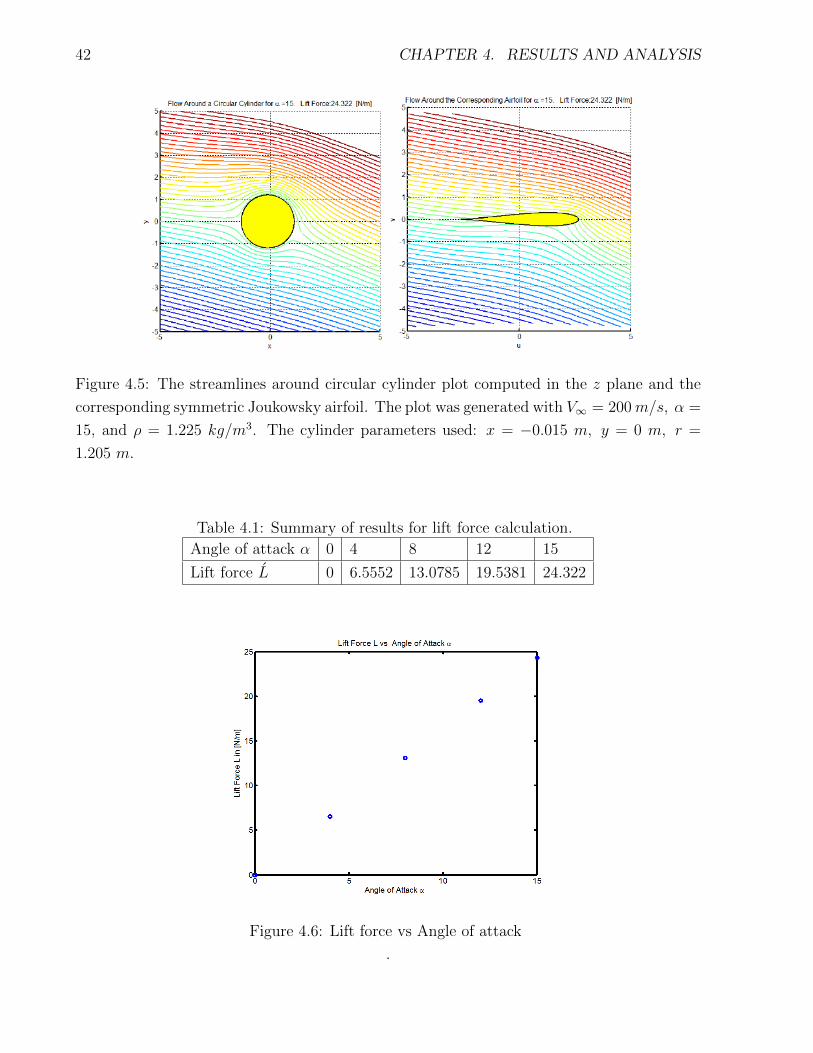
42 CHAPTER 4. RESULTS AND ANALYSIS
Figure 4.5: The streamlines around circular cylinder plot computed in the z plane and the
corresponding symmetric Joukowsky airfoil. The plot was generated with V∞ = 200m/s, α =
15, and ρ = 1.225 kg/m3. The cylinder parameters used: x = −0.015 m, y = 0 m, r =
1.205 m.
Table 4.1: Summary of results for lift force calculation.
Angle of attack α 0 4 8 12 15
Lift force L 0 6.5552 13.0785 19.5381 24.322
Figure 4.6: Lift force vs Angle of attack
.

4.1. COMPUTING THE STREAMLINES AROUNDANAIRFOIL AND LIFT CALCULATION43
Table 4.2: Summary of results for lift coefficient calculation.
Angle of attack α 0.250 1.250 2.250 3.250 4.250 5.250 6.250
CL(NACA0012) 0.0281 0.1379 0.2349 0.3545 0.4610 0.5689 0.6875
CL(JOUKOWSKY 12%) 0.0288 0.1438 0.2459 3.724 0.4853 0.5968 0.7051
Table 4.3: Summary of results for lift coefficient calculation.
Angle of attack α 7.250 8.250 9.250 10.250 11.250 12.250
CL(NACA0012) 0.8162 0.9453 1.0365 1.1288 1.2227 1.3144
CL(JOUKOWSKY 12%) 0.8145 0.9228 1.0290 1.1318 1.2301 1.3221
Figure 4.7: Comparison between Joukowsky 12% airfoil and the NACA 0012 airfoil, here we
compared the linear dependence of lift coefficient on the angle of attack for both airfoils.

44 CHAPTER 4. RESULTS AND ANALYSIS
Figure 4.8: Absolute Error in lift coefficients for Joukowsky Airfoil and actual NACA 0012
Airfoil.

Chapter 5
Conclusion
The main goal of our thesis was to apply the conformal mapping technique to model the
two dimensional fluid flow around an airplane wing. We reviewed the mathematical model
used to describe the two dimensional ideal fluid flow around a circular cylinder obtained by
the superposition of simple elementary flows. This model was implemented in MATLAB
in order to visualize the streamlines and the equipotential curves for each elementary flow
needed in the process of modeling the flow around a circular cylinder. We have used the
Joukowsky transformation to map the circular cylinder to a flat plate, an ellipse and to
the desired Joukowsky airfoil. We have established the complex potential of the lifting flow
around the circular cylinder in theorem 3.1 and it was found that the circulation and the
lift force in the z plane remained unchanged in the w plane when the complex potential
is transformed by a conformal mapping function. MATLAB software was used to compute
and visualize the streamlines around the circular cylinder and the corresponding Joukowsky
airfoil. The lift force was calculated at different angle of attack and it was found that the
lift force is strongly dependent to the angle of attack in a linear proportion as illustrated in
figure 4.6. Moreover we have compared the linear dependence of the lift coefficients on the
angle of attack for Joukowsky and NACA 0012 airfoil. And the results showed that they are
almost equivalent in the range of 0 to 12.25 degrees of the angle of attack. The plot of the
absolute error in CL was generated to show graphically the maximum absolute error in lift
coefficients for Joukowsky Airfoil and actual NACA 0012 Airfoil which is approximately 2.8%.
For further studies one can emphasize on the Karman-Trefftz transformation as an im-
proved transformations to avoid the two drawbacks of the Joukowsky airfoils. These draw-
backs include a knife-edge cusp at the trailing edge which presents manufacturing and struc-
tural integrity difficulties and the fact that the profiles of the Joukowsky airfoil have the
maximum thickness very close to the leading edge, which results in adverse pressure gradient
over most of the upper surface leading to earlier boundary layer transition and higher skin
friction drag.
45
46 CHAPTER 5. CONCLUSION
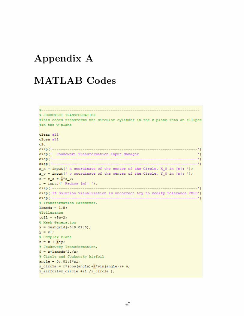
Appendix A
MATLAB Codes
47
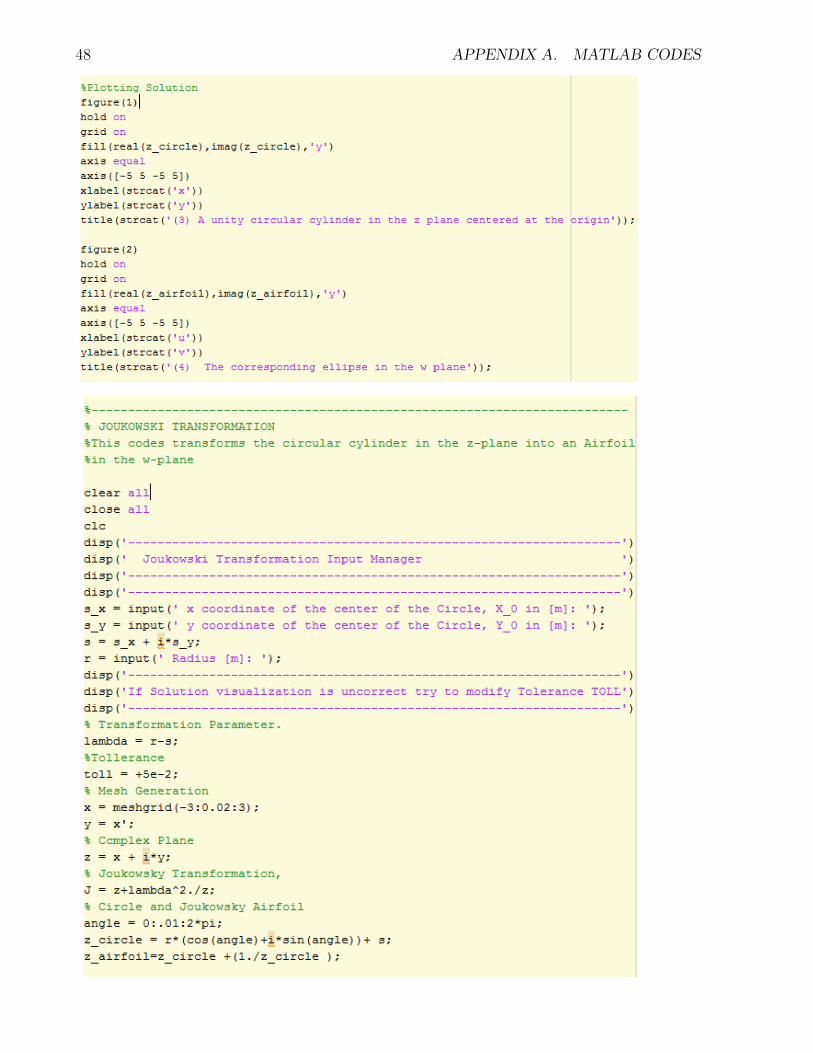
48 APPENDIX A. MATLAB CODES
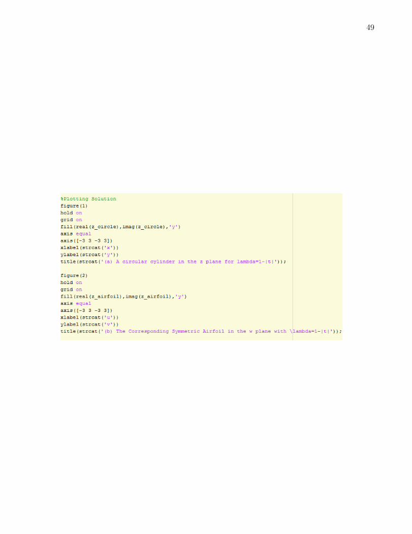
49

50 APPENDIX A. MATLAB CODES

51

52 APPENDIX A. MATLAB CODES

Bibliography
[1] R. Nitin Kapania, Katherine Terracciano, Shannon Taylor, Modeling the Fluid Flow
around Airfoils Using Conformal Mapping, August/2008.
[2] K. Tapan Senguta, Theoretical and Computational Aerodynamics, IIT Kampur, Indea,
2015.
[3] J. Mark Ablowitz, S. Athanassios Fokas, Complex Variables, Introduction and Applica-
tions Second Edition, Cambridge Tests in Applied Mathematics, Cambridge University
Press, 2003.
[4] L.M. Milne-Thomson, C.B.E.,Theoretical Aerodynamics, Fourth Edition, Dover Publi-
cations, INC. New York, 1958.
[5] J.J. Chattot, M. M. Hafez, Theoretical and Applied Aerodynamics and Related Numerical
Methods, Springer, New York, 2015.
[6] Marlies van Osch, Dynamics of a 2 D Aircraft Wing with Cavity, Test a New Experi-
mental Method, DCT 2008.035.
[7] www.dynanicsflight.com/areodynamics/airfoils/accessed on 04th/10/2017.
[8] Thomas Johnson, Conformal Mapping in Wing Aerodynamics, 2013.
[9] James Stewart, Calculus Early Transcendentals, 6th Edition, Mc M aster University,
2008.
[10] Anderson, D. John, Fundamentals of Aerodynamics, 4th Edition, New York: Mc Graw-
Hill, 2007.
[11] Nalsh, Paul, Intoduction to Conformal Mapping in Aerodynamics, Department of
Aerospace Engineering, Ryerson University.
[12] Bear, Jacob, Dynamics of Fluids in Porous, Media, Canada: American Elsevier, 1972.
[13] Katz, Joseph and Allen Plotkin, Low Speed Aerodynamics, 2nd Edition, New York:
McGraw-Hill, 1991.
53
54 BIBLIOGRAPHY
[14] Anderson, David and Scott Eberhardt, Understanding Flight, 2nd Edition, Prentice Hall,
1988.
[15] J. Benson Thomas, Interactive Educational Tool for Classical Airfoil Theory, NASA
Lewis Research Center, Cleveland, Ohio 44135, October/1996.
[16] L. Panton Ronarld, Incompressible Flow, Fourth Edition, New Jersey, 2013.
[17] Hiromichi, Yutaka hara, takafumi Kawamura,Takuju nakamura, Yeon, Seung Lee, A
Conformal Mapping Technique to Correlate the Rotating Flow Around a Wing Section of
Vertical Axis Wind Turbine and Equivalent Linear Flow Around a Static Wing, Division
of Ocean Systems Engineering, Korea Advanced Institute of Science and Technology,
November/2013.
[18] C.Ives David, A Modern look at conformal Mapping Including Multiply Connected Re-
gions, Grumman Aerospace Corporation, Bethpage, New York, August/1967.
[19] Th.Von Karman, W.R.Sears, Airfoil Theory for Non- Uniform Motion, California Insti-
tute of Technology, 1938.
[20] www.airfoiltools.com/airfoil/details?airfoil=joukowsk-il/ accessed on 18th/03/2018.
[21] D. Lysak Peter, Unsteady Lift of Thick Airfoils in Incompressible Turbulent Flow, a
PhD. Dissertation in Acoustics Submitted in Partial Fulfillment of the Requirements for
the Degree of Doctor of Philosophy, the Pennsylvania State University, May/2011.
[22] V. Pavlenko, L. Rosenqvist, O. Kochukhov, Fluid Mechanics Compendium, Department
of Physics and Astronomy, Uppsala University, September/2014.
[23] M. White Frank, Fluid Mechanics, Fourth Edition, University of Rhode Island, Mcgraw
Hill College, 1998.
[24] ALAN Pope, Basic Wing and Airfoil Theory, Fourth Edition, New York, Mcgraw Hill
book Company, INC, 1951.