APPLICATION-ORIENTED RELATIVISTIC ELECTRODYNAMICS (2) · APPLICATION-ORIENTED RELATIVISTIC ELECTRODYNAMICS (2) D. Censor Ben Gurion University of the Negev Department of Electrical

Progress In Electromagnetics Research, PIER 29, 107–168, 2000

APPLICATION-ORIENTED RELATIVISTIC

ELECTRODYNAMICS (2)

D. Censor

Ben Gurion University of the NegevDepartment of Electrical and Computer EngineeringBeer Sheva, Israel 84105

Abstract–This article is a revised and upgraded edition of a previousone published in this journal, hence the label (2), see the GeneralRemarks section below.

Relativistic Electrodynamics, for many years a purely academic sub-ject from the point of view of the applied physicist and electromagneticradiation engineer, is nowadays recognized as pertinent to many prac-tical applications. We therefore need to define a syllabus and explorethe best methods for educating future generations of such users. Suchan attempt is presented here, and is of course biased by personal pref-erences. What emerges as general guidelines are the facts that Rel-ativistic Electrodynamics should be presented axiomatically, withouttrying to “explain the physical meaning” of Special Relativity, thatfour-vectors and their mathematical properties should be emphasized,and that the field tensors, an elegant formalism, albeit of limited practi-cal use, should be avoided. Use of four-fold Fourier transforms not onlygreatly simplifies the relevant manipulations, it is also of paramountimportance for discussion of dispersive media. This approach yieldsmany concepts as mathematical results, e.g., the Relativistic Dopplereffect, which therefore do not require a long phenomenological discus-sion with many “explanations”. Introducing this approach as earlyas possible opens new vistas for the student and the educator, indeedsome of the new results here do not appear in textbooks on SpecialRelativity. One of the main results shown here is the fact that thegeneralized Fermat principle states that the ray will propagate in sucha manner that the proper time will be minimized (or extremized, ingeneral). It also strips the mystique of this principle, showing that it isin fact equivalent to a modest mathematical condition on the smooth-ness of the phase function. The presentation is constructed in a way

108 Censor

that allows the student to gradually overcome difficulties in assimilat-ing new concepts and applying them. In that too it is different frommany conventional presentations.

1. General Remarks2. Introduction and Rationale3. Traditional and Topsy-turvy Special Relativity4. Ruler and Twins Paradoxes5. Fourier Transforms and the Doppler Effect6. Invariants Galore7. Potentials8. The Cross Multiplication and Curl Operations9. Proper Time and Related Concepts10. The Breakdown of Special Relativity11. The Minkowski Constitutive Relations12. Dispersion Equations in Moving Media13. Application to Hamiltonian Ray Propagation14. The Fermat Principle and its Relativistic Connotations15. Application to Ray Theory in Lossy Media16. Nonlinear Media and Volterra Series17. Differential Operator Constitutive Relations18. Scattering by a Moving Cylinder19. Concluding RemarksReferences

1. GENERAL REMARKS

The present paper is a revision and upgrading of an article previouslypublished in this journal [1]. During almost a decade since its pub-lication, the paper [1] served as the backbone for a course by thesame name, offered numerous times to graduate students, mainly fromelectrical engineering departments, in numerous universities in manycountries. Experience, new ideas for explaining certain points, newunderstanding of the fundamentals, awareness of students’ needs —all these suggested that the time has come for an upgraded version.

The general thrust of the first version is retained. The topsy-turvyapproach to Special Relativity [2] is used, heavy mathematical tools areavoided, and only Euclidean space, mostly in Cartesian coordinates isused. Without relenting on the basic ideas and their consequences, but

Application-oriented relativistic electrodynamics (2) 109

also avoiding being bogged down in too much detail, the theoreticalsubjects and some applications are presented to the students. Presentday too practical curricula call for such conciliation with the corner-stones of our fundamental understanding of the physical world. Thegraduate program, after the chase for grades in the undergraduate hey-day is over, and before the short-term short-sighted demands of R&Dand industrial practicalities dominate the agenda, is the student’s lastchance for understanding the scientific basics of his engineering pur-suits.

Some new material has been added, to cover a diverse range of ex-amples. The velocity-dependent problem of scattering by a movingcylinder found its way into the lecture material, and new aspects re-garding nonlinear wave propagation is presented. Although not purelya relativistic problem, its presentation using Minkowskian four-vectorsis a boon. It also helps in understanding Minkowski’s methodology forconstitutive relations in moving media. Finally, also included is the re-cent subject of Volterra differential operators for constitutive relations,in media at rest and in motion.

2. INTRODUCTION AND RATIONALE

The intimate relationship between Maxwell’s theory for the electro-magnetic field and Einstein’s Special Relativity theory [3] is generallyrecognized nowadays. Throughout the present century many educa-tors found it necessary to include a chapter on Special Relativity intextbooks devoted to electromagnetic field theory, e.g., in the book byBecker, edited by Sauter [4] (a book that has its roots in the last cen-tury and appeared practically in sixteen editions!), see also Stratton[5], Fano Chu and Adler [6], Sommerfeld [7], Jordan and Balmain [8],Panofsky and Phillips [9], Shadowitz [10], Jackson [11], Portis [12], Lor-rain and Corson [13], Wangness [14], Griffiths [15], Frankl [16], Chen[17], Kong [18], Plonus [19], Eringen and Maugin [20], Schwartz [21].This list is representative, rather than exhaustive.

Last but not least, the pioneering book by Van Bladel [22] mustbe mentioned. In an attempt to serve the needs of the engineeringcommunity, the book compiles results of many relevant studies. Thetopics chosen are more or less of practical nature, related to RelativisticElectrodynamics. It is hoped that experiments like Van Bladel’s bookand the present article contribute to clarify the question of how topresent an application-oriented course of this kind to students.

110 Censor

By scrutinizing the above mentioned and other textbooks, it be-comes apparent that a specific approach suitable for educating appliedphysicists and electrical engineers, especially in the area of electromag-netic radiation engineering, is lacking. Some authors introduce SpecialRelativity theory in the traditional “Gedanken experiment” approach,and by the time the reader finishes with the moving trains, flashingtorchlights, and rods and clocks, the relevance to practical electro-magnetic problems is obscured. Others move along more formalisticlines and derive the field tensors, mostly by using general coordinatesystems and the heavy machinery of differential geometry, i.e., covari-ant and contravariant coordinate systems. Experience shows that themathematical elegance hardly provides an incentive for the engineeringstudent to move on in this field. On the other hand, we are nowadaysaware of some real-life problems, e.g., design of satellite supportedglobal navigation and positioning systems (GPS), which involve spe-cial (and sometimes even general) relativistic considerations related toprecision of time and frequency bases and errors incurred during prop-agation through complicated inhomogeneous and time varying media,and everything in the presence of relative motion between objects. Itis therefore mandatory to devise the methodological tools and suit-able representations for teaching Relativistic Electrodynamics to ap-plied physics and electrical engineering students. In the course of sucha pedagogical experiment with electrical engineering graduates, it be-came clear that the rudiments of Special Relativity should be presentedaxiomatically, with as little phenomenological “explanations” as feasi-ble, working on the assumption that this aspect has been covered atleast to some extent in “Baby physics” courses. To repeat this part ofthe story means that in a one quarter (or semester) course there mightnot be sufficient time for effectively discussing the more advanced top-ics presented here. It also became clear that four-dimensional Fouriertransforms should be introduced right from the beginning, an unortho-dox approach as far as this author is aware. This facilitates the workin an algebraic, rather than differential equations environment, thussimplifying mathematical manipulations. It also became clear thatfour-vectors, which are easily handled, almost as easily as the classicalthree-vectors, should be extensively used. Most of the students methad a fair to good grasp of vector analysis and linear algebra, and theintroduction of four-vectors and dyadics did not pose a problem. How-ever, only Euclidean systems are considered, and even in this context,


the elegance of the electromagnetic field tensors and the associatedrepresentation of Maxwell’s equations has been avoided. Within theselimits, it is then the personal preference of the teacher that will guidehim to emphasize certain classes of problems. From this point of viewthe specific material described here serves merely as an example. Butcarefully choosing the examples also serves to get some new insightinto supposedly old problems. For example, the section on the Fermatprinciple shows that the generalized principle, for inhomogeneous andtime dependent media, acquires a new meaning that can only be statedin the context of Special Relativity: Verbally stated, it says that theray propagates along a path that minimizes (or in general extremizes)the proper time. It is also shown that the Fermat principle is equiv-alent to a simple mathematical condition on the smoothness of thephase function.

The present article is organized as follows: First, Relativistic Elec-trodynamics is introduced axiomatically, using the topsy-turvy ap-proach [2]. The introduction of compact notation conventions facil-itates exploring properties of relevant Minkowski four-vectors, and adiscussion of the Lorentz transformation, the associated differential op-erators, and some important conclusions of the theory, exemplified bythe ruler, and twins, paradoxes. Then the four-dimensional Fouriertransformations are introduced, providing the technique of algebraiza-tion for the Maxwell equations. The associated spectral domain four-vector is identified as the relativistic Doppler effect. These four-foldintegrals bring up the important and nontrivial question of the validityof transformed spatiotemporal transformations formulas when statedin the spectral domain. Further exploration of four-vectors follows.Next, four-potentials are introduced. This is followed by a discussionof the cross multiplication operation and the related curl operation. Itis mentioned, without going into too much detail, that we are dealingwith tensor operations, and the general advice is to work with the var-ious components (this is done without mentioning the anti-symmetrictensors and their properties, which would encumber the presentationwithout contributing to application-oriented problems). A section onthe proper time and related concepts in mechanics follows. At thispoint a section with the provocative title “The breakdown of SpecialRelativity” is introduced. It is emphasized that for varying velocities,Special Relativity becomes a heuristic approximation, holding only forslowly accelerated objects. This observation, noted by Einstein [3],

112 Censor

somehow faded out from many later tractates and textbooks.We now have enough tools for discussing specific problems. What

might sometimes appear as a melange of unrelated subjects is actuallyan attempt to lead the student gradually from the less complicated tothe more sophisticated subjects. As a first example, the Minkowskimethodology for the constitutive relations for moving media is dis-cussed, and the derivation for homogeneous, dispersive, and anisotropicmedia is demonstrated. Dispersion equations and their relativistic in-variance are discussed. This provides the basis for discussing Hamilto-nian ray propagation for inhomogeneous and time varying dispersivemedia. This is followed by a section discussing the generalized Fermatprinciple, and its associated Euler-Lagrange equations, which are onceagain the Hamiltonian ray equations. As a further application, whichis of course biased by the author’s personal preferences, the questionof ray propagation in lossy media is discussed, in the context of theray equations, their generalization to lossy media and the questionsof Lorentz transformations and mathematical complex analyticity in-volved. The advantage of using Minkowskian four-vectors even fornon-relativistic problems is further demonstrated by the application ofthe Volterra functional series to wave propagation in nonlinear systems.The novel concept of the associated Volterra differential operators isalso introduced, for homogeneous and inhomogeneous media. FinallyRelativistic Electrodynamics is applied to the classical problem of scat-tering by a cylinder, in order to derive the formulas for scattering by amoving object. The interaction of multipolity in the result is an inter-esting consequence. Accordingly multipoles in motion acquire highermultipole modes — a monopole becomes a monopole plus a dipole, etc.Squeezing all this into a single semester course requires considerablesleight, and the extent of using these or different applications dependson the teacher, the available span of time, and the audience.

3. TRADITIONAL AND TOPSY-TURVY SPECIALRELATIVITY

In this section Relativistic Electrodynamics is introduced. The formal-ism needed by the applied physicist and engineer is stipulated in anaxiomatic manner. The introduction of the field tensors and the ensu-ing elegant representation of the field equations by means of operationson these tensors, a cornerstone of relativistic formalism, is obviated.Four-vectors in Minkowski space are introduced along the way as a no-


tational and operational tool, rather than a metaphysical-conceptualgeneralization of the space-time manifold idea, as sometimes impliedin books specializing in relativity theory. This somewhat peremptorymethodology follows the realization that we do not have the time tothoroughly plough the background knowledge, lest no time will remainto teach the pertinent engineering aspects.

Maxwell’s equations for the electromagnetic field (in the “unprimed”frame of reference denoted by Γ) are given by

∂x × E = −∂tB − jm∂x × H = ∂tD + je∂x · D = ρe

∂x · B = ρm

(1)

where ∂x (often symbolized by ∇ and called “Nabla”, or sometimes“Del”) and ∂t denote the space and time derivative operators, respec-tively. In general all the fields are space and time dependent, e.g., E= E(X). Here

X = (x, ict) (2)

symbolizes the space-time dependence, actually X denotes the event(world point) in the sense of a Minkowski-space location vector, as dis-cussed below, where c is the universal constant of the speed of light,and i is the unit imaginary complex number i2 = −1 . For symmetryand completeness, in the present representation, the Maxwell equationsinclude the usual electric (index e) , as well as the fictitious magnetic(index m) , current and charge density sources. To date, the existenceof the magnetic current and charge densities in (1) has not been empir-ically established. Therefore at this time they should be considered asfictitious, in the sense that they are auxiliary and not intrinsic physicalentities. Magnetic currents and charges are amply used in a varietyof practical problems to emulate equivalent sources, e.g., when surfacesources are designed to satisfy certain discontinuities in the fields. SeeLindell [23], Stratton [5], or Kong [18], as well as many other text-books cited above. However, we should always be aware of the factthat physicists have not given up the quest for magnetic charges andcurrents, e.g., see Jackson [11].

The statement of Maxwell’s equations (1) is incomplete in the sensethat it is unrelated to the rest of physics. For example, we need a wayof linking Electrodynamics to familiar concepts like force and energy

114 Censor

introduced in the context of mechanics. One way of achieving thisgoal is by stating a force formula. Thus the presence of a conventionalcharge qe can be detected through the forces exerted on it accordingto the Lorentz force formula

fe = qe(E + v × B) (3)

The teaching of electromagnetic theory in a phenomenological-historical way, as evolving from crucial experiments and the conse-quent “laws” that are added into the model, tends to obscure the factthat (3) is extrinsic and does not follow from Maxwell’s equations.This important fact should be stressed at this point. Actually (3) is anextension of the simple Coulomb force formula fe = qeE which shouldbe considered not as a “law” but as a link between mechanics andElectrodynamics. Inasmuch as fe is supposedly already known frommechanics, fe = qeE can be considered as a definition of the propor-tionality coefficient qe . Once it is defined we have at our disposal the“rationalized” Giorgi MKSQ system of units. On introducing SpecialRelativity axiomatically, (3) can be derived from fe = qeE . Inspiredby symmetry considerations, the analog of (3) for magnetic sources isassumed to be

fm = qm(H − v × D) (4)again an extension derived by means of relativistic transformation for-mulas given below from a magnetic force formula fm = qmH . Al-though this example is far fetched, it demonstrates the symmetry in-troduced into Maxwell’s equations by stipulating magnetic sources,and the stimulus it provides for looking at things in a new way.

Special Relativity theory, dealing with observations performed ininertial systems, i.e., frames of reference in relative uniform motion,has been announced by Einstein [3], however he considers there onlyfree space (“vacuum”) electrodynamics.

Einstein’s Special Relativity theory (relevant statements are de-noted by S for “Special”) postulates:

(S-1). Light speed c is a universal constant observed in all inertialframes.

(S-2). Maxwell’s equations provide the model or “law of nature”for describing the electromagnetic field. I.e., the theory recognizes (1)above.

(S-3). Maxwell’s equations existing for all observers in inertial fra-mes of reference have the same functional structure (henceforth: Co-variance). This means that if (1) exists for an observer in one frame of


reference, in another inertial frame (the “primed” frame of referenceΓ′) , Maxwell’s equations have the form:

∂x′ × E′ = −∂t′B′ − j′m∂x′ × H′ = ∂t′D′ + j′e∂x′ · D′ = ρ′e∂x′ · B′ = ρ′m

(5)

where now E′ = E′(X′) , and the native, or proper, space-time coor-dinates in the Γ′ system are denoted by X′ = (x′, ict′) , which is alsoa Minkowski locational four-vector.

The consequences of the above three postulates follow:(S-i). From (S-1), i.e., the constancy of the speed of light, the

Lorentz space-time transformations X′ = X′[X] , mediating betweenspatiotemporal coordinates in Γ and Γ′ are developed in the form:

x′ = U · (x − vt)

t′ = γ(t − v · x/c2

) (6)

Here v is the velocity by which Γ′ is moving, as observed from Γ , andwe define

γ = (1 − β2)−1/2, β = ν/c, ν = |v|,U = I + (γ − 1)vv, v = v/ν

(7)

where the tilde denotes dyadics. Briefly, a dyadic is just a differentnotation for a matrix, or in general, a tensor, and very convenientto use in conjunction with vectors. E.g., a dyadic can be created byjuxtaposed vectors (or a linear combination of such) without a dotor cross multiplication sign between them, amounting to an externalproduct of matrices. Here I is the idemfactor or unit Dyadic (sameas unit matrix). From (6) and the chain rule of calculus follows thetransformation ∂X′ = ∂X′ [∂X] for the space-time differential operators,

∂x′ = U ·(∂x + v∂t/c2

)

∂t′ = γ(∂t + v · ∂x)(8)

and compacted in a four-vector form

∂X =(

∂x,−i

c∂t

)

(9)

116 Censor

is the four-gradient operator. How a quadruplet like (9) is tested toqualify as a proper Minkowski four-vector is discussed below.

(S-ii) From the axioms (S-2), (S-3) above, the transformation for-mulas for the fields in Γ and Γ′ are derived in the following form:

E′ = V · (E + v × B)

B′ = V ·(B − v × E/c2

)

D′ = V ·(D + v × H/c2

)

H′ = V · (H − v × D)

V = γI + (1 − γ)vv

(10)

where E′ = E′(X′) and E = E(X) , etc., and the Lorentz transfor-mation (6) is identically satisfied X′ ≡ X′[X] by the spatiotemporalcoordinates indicated in (10). Similarly, for the sources we derive thetransformation formulas:

j′e,m = U · (je,m − vρe,m)

ρ′e,m = γ(ρe,m − v · je,m/c2

) (11)

for the corresponding e-, or m-, indexed sources.Topsy-turvy (T) Special Relativity is stated in inverse order:(T-1) Instead of assuming the constancy of the speed of light (S-l

above), we assume the validity of the Lorentz transformation (S-i), i.e.,(6).

(T-2) Here too we start with the same postulate (S-2) on the validityof equation (1).

(T-3) We postulate the validity of the formulas for the transforma-tions of fields as given by (9), (10), i.e., what above constituted (S-ii).

The consequences are:(T-i) From (T-1) we derive the constancy of c , the speed of light,

i.e., (S-1) in the first model.(T-ii) From (T-1), i.e., (6), (8) and (T-2), (T-3) we derive the co-

variance of Maxwell’s equations, i.e., (S-3) of the previous model.One might argue that the present model loses the motivation for

universality and simplicity, displayed in the S-model. While this mightbe a valid argument, nevertheless it is compensated by the fact thatthe T-model is much easier to handle in the classroom, and the S-model can be mentioned in retrospect, showing how the two modelsare equivalent.


It is easily verified that the inverse transformation is obtained frome.g., (6), (8), (10), (11) by exchanging primed and unprimed symbolsand inverting the sign of v. This is also valid for other transformationsgiven below.

This, in a nutshell, is the basis of Special Relativistic Electrodynam-ics. Some brief references will be made below regarding RelativisticMechanics.

Note that U · V = γI . Also interesting are the roles of the dyadicsU , V , in sorting out the components of the three-dimensional vectorsinto parallel and perpendicular components with respect to the velocityv and multiplying by γ . The product of U , V and a vector attachesa factor γ to the parallel, perpendicular, component of the vector, re-spectively. Of course we know that the reason for a three dimensionalvector to be associated with either U , or V depends whether it isa “true” vector, i.e., the spatial part of a four-vector, like x or j ,or a component of an antysymmetrical tensor, like E, B, D, H , re-spectively. Exactly this is the part of the story that we should avoiddiscussing with students novices, to the subject of Relativistic Electro-dynamics, and present the theory axiomatically. The finer details canwait for a later encounter with this material.

Minkowski [24] introduced the four-vector concept which will enableus to compact our notation and simplify the algebraic and differen-tial manipulations. To the three components xj , j = 1, 2, 3 we addx4 = ict , thus for real t we have now an imaginary coordinate x4 .Henceforth four-vectors will be denoted by capital boldface characters,like in (2) and (9). It is not necessary at this stage to introduce thegeometrical concepts pertaining to the Minkowski space, i.e., to de-scribe the Lorentz transformation as a rotation in this space. Whatis important for the student to know is the fact that the length of afour-vector is invariant with respect to the Lorentz transformation (6).It can be verified as an exercise that subject to (6)

X · X = x · x − c2t2 = X′ · X′ = x′ · x′ − c2t′2 (12)

This also explains how a four-vector scalar product is obtained. In thespecific case that in (12) a constant value is chosen, it must be a zero.The reason is simple: Our specific choice of the Lorentz transformationin the form (6) prescribes that at t = t′ = 0 also x = x′ = 0 , hencefor this specific case

X · X = X′ · X′ = 0 (13)

118 Censor

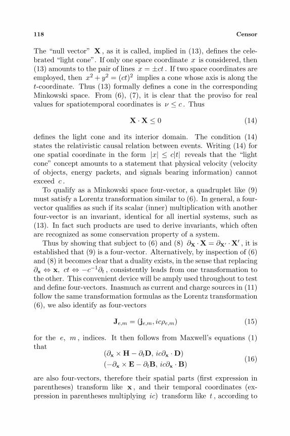
The “null vector” X , as it is called, implied in (13), defines the cele-brated “light cone”. If only one space coordinate x is considered, then(13) amounts to the pair of lines x = ±ct . If two space coordinates areemployed, then x2 + y2 = (ct)2 implies a cone whose axis is along thet-coordinate. Thus (13) formally defines a cone in the correspondingMinkowski space. From (6), (7), it is clear that the proviso for realvalues for spatiotemporal coordinates is ν ≤ c . Thus

X · X ≤ 0 (14)

defines the light cone and its interior domain. The condition (14)states the relativistic causal relation between events. Writing (14) forone spatial coordinate in the form |x| ≤ c|t| reveals that the “lightcone” concept amounts to a statement that physical velocity (velocityof objects, energy packets, and signals bearing information) cannotexceed c .

To qualify as a Minkowski space four-vector, a quadruplet like (9)must satisfy a Lorentz transformation similar to (6). In general, a four-vector qualifies as such if its scalar (inner) multiplication with anotherfour-vector is an invariant, identical for all inertial systems, such as(13). In fact such products are used to derive invariants, which oftenare recognized as some conservation property of a system.

Thus by showing that subject to (6) and (8) ∂X ·X = ∂X′ ·X′ , it isestablished that (9) is a four-vector. Alternatively, by inspection of (6)and (8) it becomes clear that a duality exists, in the sense that replacing∂x ⇔ x, ct ⇔ −c−1∂t , consistently leads from one transformation tothe other. This convenient device will be amply used throughout to testand define four-vectors. Inasmuch as current and charge sources in (11)follow the same transformation formulas as the Lorentz transformation(6), we also identify as four-vectors

Je,m = (je,m, icρe,m) (15)

for the e, m , indices. It then follows from Maxwell’s equations (1)that

(∂x × H − ∂tD, ic∂x · D)(−∂x × E − ∂tB, ic∂x · B)

(16)

are also four-vectors, therefore their spatial parts (first expression inparentheses) transform like x , and their temporal coordinates (ex-pression in parentheses multiplying ic) transform like t , according to


(6). This provides another example for constructing a four-vector, andfrom the covariance of the Maxwell equations (S-3) or (T-ii), (16) interms of Γ′ fields is valid too.

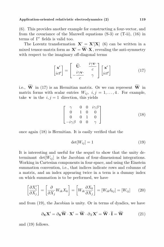
The Lorentz transformation X′ = X′[X] (6) can be written in amixed tensor-matrix form as X′ = W·X , revealing the anti-symmetrywith respect to the imaginary off-diagonal terms

[x′

ict′

]

=

U· iγv·

c

− iγv·c

γ

[x′

ict′

]

(17)

i.e., W in (17) is an Hermitian matrix. Or we can represent W inmatrix forms with scalar entries Wij , i, j = 1, . . . , 4 . For example,take v in the i, j = 1 direction, this yields

γ 0 0 iγβ0 1 0 00 0 1 0

−iγβ 0 0 γ

(18)

once again (18) is Hermitian. It is easily verified that the

det[Wij ] = 1 (19)

It is interesting and useful for the sequel to show that the unity de-terminant det[Wij ] is the Jacobian of four-dimensional integrations.Working in Cartesian components in four-space, and using the Einsteinsummation convention, i.e., that indices indicate rows and columns ofa matrix, and an index appearing twice in a term is a dummy indexon which summation is to be performed, we have

[∂X ′

i

∂Xj

]

=[

∂

∂XjWikXk

]

=[

Wik∂Xk

∂Xj

]

= [Wikδkj ] = [Wij ] (20)

and from (19), the Jacobian is unity. Or in terms of dyadics, we have

∂XX′ = ∂XW · X′ = W · ∂XX′ = W · I = W (21)

and (19) follows.

120 Censor

4. RULER AND TWINS PARADOXES

These subjects provide some deeper insight into the implications of theLorentz transformation, as well as some exercise in the manipulationof the formulas.

For the ruler paradox, we assume a ruler of length L , which wewould like to pass through a slit of length l . If l < L and no tilting isallowed the mission cannot be accomplished. So here Special Relativitycomes to the rescue: Let us move back, and set the ruler in motionat a velocity v parallel to the ruler and the slot. The ruler will nowbe of length L as observed in the co-moving frame of reference Γ′ .But in the slot’s system of reference Γ , length contraction occurs, dueto the factor γ in the Lorentz transformation (6). The observer in Γwaits until the seemingly shortened ruler is above the slot, and jerksit down. The mission is accomplished, or is it? The paradox stemsfrom the fact that the observer in Γ′ predicts a similar shortening, ofthe relatively moving slot, which makes the situation even worse! Therelevant one-dimensional form of (6) is now given by

x′ = γ(x − νt)

t′ = γ(t − xν/c2)(22)

At time t′ = t = 0 the two systems coincide at x′ = x = 0 . Letus assume x′ = x = 0 to be aligned to the trailing edge of the ruler.At this time t = 0 other points are related through x′ = γx . If att = 0 the leading edge is in Γ′ at x′ = L , this then corresponds tox = L/γ in Γ . If x = l ≥ L/γ , then the ruler can pass through theslot. However, from the second equation (22) it follows that for theobserver this happens at an earlier time t′ = −γxν/c2 . Specificallyat t′ = −Lν/c2 . So, from the point of view of the Γ′ observer, theleading edge goes under the table at t′ = −Lν/c2 , the trailing edgefollows at t′ = 0 . If the thickness of the table and the ruler are zero,there is no tilting. So much for the ruler paradox.

The twins paradox is even more exciting: Assume two twins identi-cal in every respect, which for our story means that they have the sameexpected life span. While one brother stays at home, the other travels,and thus undergoes a time dilatation (i.e., his clock is slower). Re-turning home, the traveling brother is younger (his aging was slower),compared to the brother that stayed at home. Since Special Relativityteaches us that all inertial systems are equivalent, why is it one twin


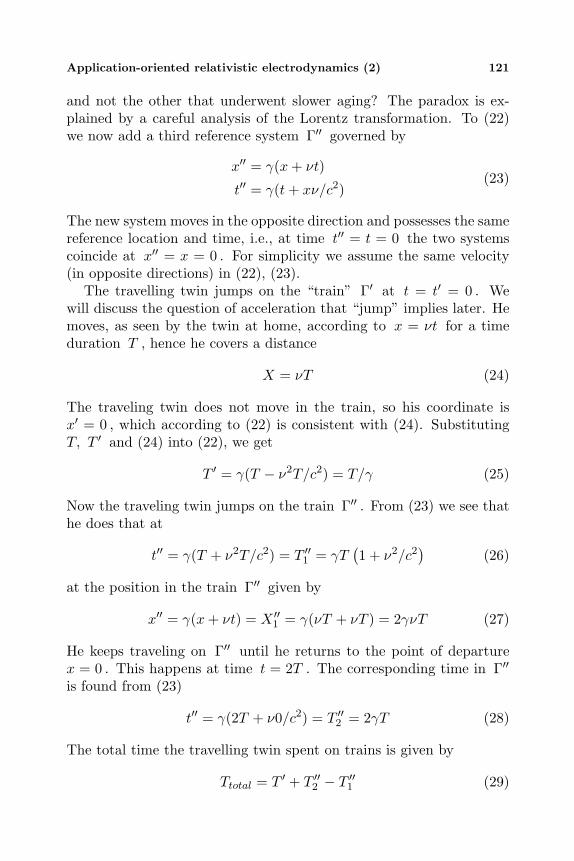
and not the other that underwent slower aging? The paradox is ex-plained by a careful analysis of the Lorentz transformation. To (22)we now add a third reference system Γ′′ governed by

x′′ = γ(x + νt)

t′′ = γ(t + xν/c2)(23)

The new system moves in the opposite direction and possesses the samereference location and time, i.e., at time t′′ = t = 0 the two systemscoincide at x′′ = x = 0 . For simplicity we assume the same velocity(in opposite directions) in (22), (23).

The travelling twin jumps on the “train” Γ′ at t = t′ = 0 . Wewill discuss the question of acceleration that “jump” implies later. Hemoves, as seen by the twin at home, according to x = νt for a timeduration T , hence he covers a distance

X = νT (24)

The traveling twin does not move in the train, so his coordinate isx′ = 0 , which according to (22) is consistent with (24). SubstitutingT, T ′ and (24) into (22), we get

T ′ = γ(T − ν2T/c2) = T/γ (25)

Now the traveling twin jumps on the train Γ′′ . From (23) we see thathe does that at

t′′ = γ(T + ν2T/c2) = T ′′1 = γT

(1 + ν2/c2

)(26)

at the position in the train Γ′′ given by

x′′ = γ(x + νt) = X ′′1 = γ(νT + νT ) = 2γνT (27)

He keeps traveling on Γ′′ until he returns to the point of departurex = 0 . This happens at time t = 2T . The corresponding time in Γ′′

is found from (23)

t′′ = γ(2T + ν0/c2) = T ′′2 = 2γT (28)

The total time the travelling twin spent on trains is given by

Ttotal = T ′ + T ′′2 − T ′′

1 (29)

122 Censor

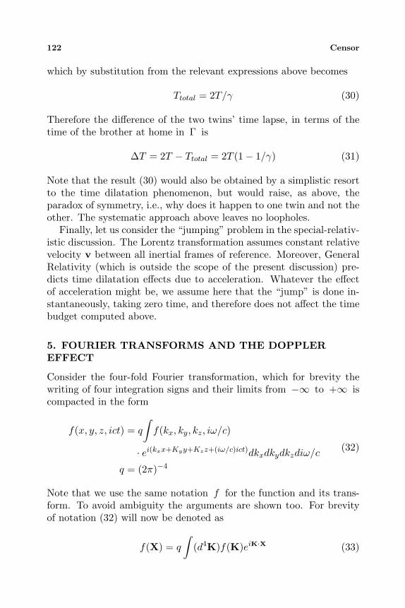
which by substitution from the relevant expressions above becomes

Ttotal = 2T/γ (30)

Therefore the difference of the two twins’ time lapse, in terms of thetime of the brother at home in Γ is

∆T = 2T − Ttotal = 2T (1 − 1/γ) (31)

Note that the result (30) would also be obtained by a simplistic resortto the time dilatation phenomenon, but would raise, as above, theparadox of symmetry, i.e., why does it happen to one twin and not theother. The systematic approach above leaves no loopholes.

Finally, let us consider the “jumping” problem in the special-relativ-istic discussion. The Lorentz transformation assumes constant relativevelocity v between all inertial frames of reference. Moreover, GeneralRelativity (which is outside the scope of the present discussion) pre-dicts time dilatation effects due to acceleration. Whatever the effectof acceleration might be, we assume here that the “jump” is done in-stantaneously, taking zero time, and therefore does not affect the timebudget computed above.

5. FOURIER TRANSFORMS AND THE DOPPLEREFFECT

Consider the four-fold Fourier transformation, which for brevity thewriting of four integration signs and their limits from −∞ to +∞ iscompacted in the form

f(x, y, z, ict) = q

∫

f(kx, ky, kz, iω/c)

· ei(kxx+Kyy+Kzz+(iω/c)ict)dkxdkydkzdiω/c

q = (2π)−4

(32)

Note that we use the same notation f for the function and its trans-form. To avoid ambiguity the arguments are shown too. For brevityof notation (32) will now be denoted as

f(X) = q

∫

(d4K)f(K)eiK·X (33)


where X is given in (2) and

K = (k, iω/c) (34)

is formally written as a four-vector, although at this stage we still needto show that it actually is a Minkowski four-vector. The integrationfour-volume element (d4K) becomes clear upon comparing (33) and(32). In an obvious manner, the associated inverse transformation isgiven by

f(K) =∫

(d4X)f(X)e−iK·X (35)

Now apply the four-dimensional gradient operation (9) to (33). Wethen obtain

∂Xf(X) = q

∫

(d4K)f(K)iKeiK·X (36)

In view of the four-gradient operator on the left, (36) constitutes a four-vector expression. This implies that K , (34), is indeed a four-vector.By inspection of (2), (6) and (34), one derives the transformation for-mulas K′ = K′[K]

k′ = U·(k − vω/c2)ω′ = γ(ω − v · k)

(37)

This is the relativistic Doppler effect first announced by Einstein [3].How many rivers of ink have flown in order to “explain” the rela-tivistic Doppler effect and the concept of “Phase invariance”! All thisbecomes superfluous when the present systematic approach is adopted.From the associated inverse Fourier transformation (35) one is led toconstruct the analog of (8), (9) in K space, thus obtaining anotherfour-vector differential operator

∂K = (∂k,−ic∂ω) (38)

and the associated transformation formulas

∂k′ = U · (∂k + v∂ω)

∂ω′ = γ

(

∂ω +1c2

v · ∂k

) (39)

which we could of course derive directly from (37) by using the chainrule of calculus.

124 Censor

Obviously this is a two way street: We could have started from theDoppler effect (37), and through the Fourier transformation arrive atthe Lorentz transformation (6). Therefore, without losing its generalproperties, the theory of Special Relativity could have been startedin the spectral domain (actually, the question of the roles of the spa-tiotemporal and spectral domains is much broader, and quite loadedwith philosophical questions, see [25, 26]).

At this point it is worthwhile to realize that indeed this was thecase, in a sense: Abraham [27], see also Pauli [28], before the advent ofEinstein’s theory [3], already derived the relativistically correct resultsfor reflection by a moving mirror.

Subjecting Maxwell’s equations (1), (5) to the Fourier transforma-tion (33) yields algebraic equations which are often easier to manip-ulate. This is achieved by replacing components of ∂X by the corre-sponding components of iK . Thus applying the Fourier transforma-tion (33) to (1) yields

ik × E = iωB − jmik × H = −iωD + jeik · D = ρe

ik · B = ρm

(40)

where the transformed fields E = E(K) etc. are understood. We canof course apply the Fourier transformation also to (5) and obtain in aconsistent manner

ik′ × E′ = iω′B′ − j′mik′ × H′ = −iω′D′ + j′eik′ · D′ = ρ′eik′ · B′ = ρ′m

(41)

and here E′ = E′(K′) etc. A cardinal question arising at this pointis whether the field transformation formulas (10), (11) hold in thespectral domain K too, and in what sense? Transforming the twosides of the first equation (10), we now get,

E′(X′) = V · (E(X) + v × B(X)) = q

∫

(d4K′)E′(K′)eiK′·X′

= q

∫

(d4K)V · [E(K) + v × B(K)]eiK·X (42)


and the question before us is whether the integrands are identical,which is not obvious, [29]. By identifying the dummy integration vari-ables as the proper spectral domain variables, obeying K′ = K′[K] asabove in (37), the exponentials become identical, because the scalarproduct K′ ·X′ = K ·X is a Minkowski space invariant. This is some-times referred to as the “phase invariance principle”, although in thepresent context of Minkowskian four-vectors it is quite trivial. Fur-thermore, it is easily shown that the change of variable in the integrals(42) involves a Jacobian whose value is unity, just like in (20), (21),K′ = K′[K] = W · [K] and therefore

d4K′ = det[∂KK′] d4K = d4K (43)

Consequently (42) can be recast as

∫

(d4K)[

E′(K′) − V · (E(K) + v × B(K))]

eiK·X = 0 (44)

implying that the expression in brackets in (44) vanishes, hence itis established that the transformation formulas (10), (11) hold in Kspace too.

Corresponding to (43) we also derive

d4X′ = det[∂xX′] d4X = d4X (45)

The results (43), (45) are usually phrased in the Special Relativityjargon as saying that “the four-dimensional volume element is a rel-ativistic invariant”. This is of course true only in the strict sense ofperforming the change of variables as above. These statement holdsfor any four-vector space, e.g., a representation space can be assignedto Je, Jm , and volume elements be defined, (d4Je), (d4Jm) , whichwill also be relativistic invariants in this sense. All this is of coursewell known, e.g., see Pauli [28], the difficulty is in explaining it to ourapplication-oriented students in a simple and coherent manner. OnceMaxwell’s equations and the field transformation formulas are availablein algebraic form, it becomes much easier to manipulate the expression,e.g., to verify the Maxwell’s equations covariance, i.e., showing that bysubstitution of the K space field transformation formulas (10), (11)into the unprimed set of Maxwell’s equation (40), the primed set (41)is obtained.

126 Censor

6. INVARIANTS GALORE

In a sense, all physical laws and models are declarations about theinvariance of certain quantities. Conservation laws are obviously inthis category, but many other properties, e.g., symmetry in whateversense, is also a declaration that something is unaffected, or conserved,or invariant, subject to some operation. Even writing a mathematical(algebraic, differential, integral etc.) equation for a physical law, suchthat everything appears on the left and is equal to zero or a constantor a unity dyadic, etc., on the right, is a declaration that “something”(the expression on the left) possesses some immutable properties.

The scalar product of two four-vectors is one way of deriving Lorentzinvariants, some of them have been recognized as fundamental “laws”,others are less important, but stand by for whenever they might beused. Thus (13) is a cornerstone of Special Relativity theory. Not lessimportant is the fact that the D’Alembert operator

∂X · ∂X = ∂x · ∂x − c−2(∂t)2 (46)

is a Lorentz invariant. Another invariant that has been elevated to thestatus of “law” is the equation of continuity

∂X · J(X) = ∂x · j(X) + ∂tρ(X) = O (47)

resulting from a divergence ∂x· operation on the first, second equationof (1) and substitution of the fourth, third equations, respectively. In(47) the corresponding electric or magnetic sources are understood.Clearly if (47) vanishes in one inertial system, it vanishes in all, becauseof the invariant nature of (47). The same conclusion is reached byapplying the divergence ∂x′ · to (5). It follows of course that in thespectral domain K the corresponding relations

K · J(K) = k · j(K) − ωρ(K) = 0 (48)

hold in all inertial systems of reference.Although the following invariant (note that it is not zero as in (47),

(48))∂K · J(K) = ∂k · j(K) + c2∂ωρ(K) (49)

is not recognized as a “law”, I would like my students to be able to seethat (49) follows from (35) by identifying f with J and multiplying


both sides by −iX , which is equivalent to taking the K space four-gradient derivative ∂K on both sides of (35).

We have already introduced many four-vectors, e.g.,

X, ∂X,Je, ∂Je ,Jm, ∂Jm ,K, ∂K (50)

including (16), and many more that are introduced below or elsewhere.Needless to say that linear combinations of invariants, operations like(49) acting on four-vectors, and so on, also yield invariants, hence weare dealing with an infinite group. Another way of deriving invariantsis through the field transformation formulas in (10). Of course this isrelated to the properties of the field tensors, but can be easily verifieddirectly. Thus we have [5] the following expressions

c2B · B − E · E = c2B′ · B′ − E′ · E′

H · H − c2D · D = H′ · H′ − c2D′ · D′

B · E = B′ · E′

H · D = H′ · D′

B · H − E · D = B′ · H′ − E′ · D′

c2B · D + E · H = c2B′ · D′ + E′ · H′

(51)

Still another way for deriving invariants through the Jacobian deter-minant is shown above (43), (45).

7. POTENTIALS

As a variation on the theme, the potentials will be discussed in thecontext of the Fourier transformed algebraic Maxwell equations. Theoriginal equations are split into two sets of fields one driven by je, ρe ,the other by je, ρm . This yields

ik × Ee = iωBe

ik × He = −iωDe + jeik · De = ρe

ik · Be = 0

∣∣∣∣∣∣∣∣∣

ik × Em = iωBm − jmik × Hm = −iωDm

ik · Dm = 0ik · Bm = ρm

(52)

respectively, where Ee = Ee(K) etc. Corresponding to (52) thereexists in the primed frame of reference Γ′ a set of Maxwell’s equations

128 Censor

with primed symbols. The transformation formulas relating K andthe fields in both frames are given above. The students are moreacquainted with the e-indexed set in (52). The relation between thetwo sets follows from the formal similarity and leads to the followingduality “dictionary”. By substitution according to this dictionary weobtain the e-indexed set of Maxwell’s equations from the m-indexedone, and vice-versa:

je ⇔ −jmρe ⇔ −ρm

Ee ⇔ Hm

He ⇔ Em

Be ⇔ −Dm

De ⇔ −Bm

Ae ⇔ −Am

φe ⇔ −φm

Φe ⇔ −Φm

(53)

In (53) the potentials have been included, defined according to

Be = ik × Ae

Ee = −ikφe + iωAe

Φe =(

Ae,i

cφe

)

∣∣∣∣∣∣∣∣∣

Dm = ik × Am

Hm = ikφm − iωAm

Φm =(

Am,i

cφm

) (54)

In (54) the potentials have been formally grouped into two four-vectors,essentially having the same structure as K , (34). Note that dimension-ally A = φ/c hence there exists no other alternative for groupingthese terms. It therefore follows from (37) that the associated trans-formation formulas should be

A′e,m = U ·

(Ae,m − vφe,m/c2

)

φ′e,m = γ(φe,m − v · Ae,m)

(55)

for the e, m indices correspondingly.It should be emphasized that the way the four-potentials (54) are

introduced is a definition, rather than a consequence. These defini-tions imply (55) and guarantee that Φe, Φm are indeed four-vectors.Therefore Φe · Φe, Φm · Φm and Φe · Φm as well as any product with


any other four-vectors constitute new Lorentz invariants. As before,some are more interesting, others do not seem to have an immediateapplication. Noteworthy is the invariant

K · Φe = k · Ae −ω

c2φe (56)

and the m -indexed analog. In free space c−2 = µoεo hence if the valueof the invariant (56) is set to zero, it becomes the well-known Lorentzcondition (in K space). However, in material media (56) ceases to bethe Lorentz condition. This is a point that might cause some confusion,especially in view of the fact that the Lorentz condition is a gaugetransformation invariant, as explained in many of the textbooks citedabove.

8. THE CROSS MULTIPLICATION AND CURLOPERATIONS

Teachers of a first course in electromagnetic field theory at sophomoreor junior level are aware of the fact that vector analysis, in particularthe Curl operation, are a major stumbling block for most students.Witness the long introductory chapters or detailed appendices in mosttextbooks. Suddenly, after some assimilation of the new concepts tookplace, they are told in the context of Relativistic Electrodynamics thatthe Curl operation is “not really a vector operation”, actually an asym-metric tensor with certain properties. In a short and condensed courseit was found expedient to keep tensor analysis and the formal detailsto the absolutely necessary minimum. Thus we already know thattwo juxtaposed vectors AB constitute a dyadic, or a matrix withcomponents AiBj . It is easy to see that a construct AiBj − AjBi

is an antisymmetric matrix. This defines the Curl operation in gen-eral, where we now have Ai = ∂xi . For i, j = 1, 2, 3 , there are onlythree independent entries in the matrix, therefore the Curl operationin three dimensional space could be disguised as a vector operation,on the other hand in four dimensional space i, j = 1, 2, 3, 4 , there aresix independent entries, therefore there is no way that such an entitycould be represented as a four-vector. This discussion is consideredsufficient for a first course in applied Relativistic Electrodynamics.

There are many cases where the six equations AiBj − AjBi = 0 ,i, j = 1, 2, 3, 4 must be satisfied. There is no harm in symbolicallywriting A × B = 0 , or ∂X × A = 0 , as long as we know what we are

130 Censor

doing. This facilitates a mental association to already known concepts,such as ∂x×∂xa = 0 where a is a scalar field. Similarly ∂X×∂Xa = 0will be understood as

∂

∂Xi

∂a

∂Xj

− ∂

∂Xj

∂a

∂Xi

= 0, i, j = 1, 2, 3, 4 (57)

and it is seen that for a smooth function a , such that the order ofdifferentiation is commutative, (57) is identically satisfied. The analogycannot be taken too far, for example the analog ∂X · ∂X × A = 0 ,when A is a four-vector, does not exist. Simple examples X × X =0 , ∂X × X = 0 , are easily verified. We can also apply the ∂X×operation to Φe, Φm , to show that this yields the Maxwell’s equationsfields appearing in (54). The details will be left for the reader to beworked out. The operation ∂X× applied to a four-vector yields sixindependent equations. This is sometimes referred to as a six-vector[7]. For more detail and the relation to the electromagnetic tensor, seefor example [5, 7]. The formal elegance of Relativistic Electrodynamicsis an aspect which should be sacrificed here in order to be able to focuson some applications.

9. PROPER TIME AND RELATED CONCEPTS

In a subsequent section ray equations are considered. The concept ofa ray is intimately associated with wave packets and their motion inspace. For that and other purposes we have to include a short sectionon the concept of proper time and related concepts of velocity andacceleration. Actually it is also warranted on ground of intrinsicallyinvolving an ingenious idea due to Minkowski: The creation of newfour-vectors by associating four-vectors with invariants, e.g., differen-tiating X with respect to the proper time to derive the four-velocity,as done below.

In analogy with a three-dimensional space we define the Minkowskispace four-dimensional arc length dS in terms of four-vectors

dS =√

dX · dX =√

dx · dx − c2(dt)2 (58)

and this is an invariant. Using (58) we further define an invarianthaving the dimensionality of time

dτ =dS

ic= dt

√

1 − dx · dxc2(dt)2

= dt′√

1 − dx′ · dx′

c2(dt′)2(59)


We now introduce the proper time τ . In (59) we attribute dτ tothe time increment of an observer co-moving with (i.e., at rest in) theprimed frame of reference Γ′ .

Consequently in (59) dx′ = 0 , i.e., dτ = dt′ . The inertial frame Γ′

is observed from Γ to be moving at the velocity u = dx/dt , hence

dτ = dt

√

1 − dx · dxc2(dt)2

= dt

√

1 − u · uc2

= dt/γ (60)

This is the celebrated relativistic time dilatation phenomenon, alreadymentioned above in connection with the twin paradox. We used ufor the relative velocity, because v is used below for the velocity as ageneral concept.

The four-velocity is now defined as

V =dXdτ

=(

dxdτ

, icdt

dτ

)

=dt

dτ

(dxdt

, ic

)

=dt

dτ(v, ic) = γ(v, ic) (61)

If v is a constant velocity and we consider the proper frame in whichv = 0 , which also implies u = 0 , then (61) reduces to the temporalcomponent ic , and the four-velocity is now an imaginary constant.The length of the four-velocity vector is therefore given by

V · V = V′ · V′ = −c2 (62)

for all observers in inertial systems. By taking differentials of theLorentz transformation (6) (using u for the relative velocity betweenframes of reference) and taking the ratio of the two equations, it isestablished that the relativistic transformation formula for v is givenby

v′ =U · (v − u)

γ(1 − v · u/c2)(63)

We could also consider the similarity of the four-vectors V =(

dxdτ , ic dt

dτ

)

and (2), and by inspection of (6) derive

dx′

dτ= U ·

(dxdτ

− udt

dτ

)

dt′

dτ= γ

(dt

dτ− u · dx

c2dτ

) (64)

132 Censor

the same way the transformations (8), (11), (37), (39), (55) were de-rived by inspection. Obviously by dividing the two equations (64), (63)is obtained once more.

The process of creating such new four-vectors can be continued. Wedefine the four-acceleration as

W =dVdτ

=(

d2xdτ2

, icd2t

dτ2

)

(65)

and similarly to (64), the pertinent transformation formulas can bederived. It is an interesting result that subject to (62) the followinginvariant vanishes

V · W = V · dVdτ

=12

d|V|2dτ

= −12

dc2

dτ= 0 (66)

i.e., the two four-vectors are always perpendicular, in a formal sense. Inthis context the phrase “relativistic acceleration is always centrifugal”is sometimes found.

It is not our intention to discuss in detail Relativistic Mechanics,because this will once again divert us from the main theme. It is how-ever straightforward to associate with the four-velocity the momentum-energy four-vector

P = mV (67)

where the proportionality factor m is the rest mass of a particle, mea-sured by an observer at rest with respect to the object. The associatedinvariant is probably the popularly best known result of Special Rela-tivity (e.g., see [30])

−c2P · P = γ2m2c4 − γ2m2ν2c2 = −c2P′ · P′ = m2c4 (68)

where in (68) the primed frame of reference Γ′ has been chosen as theco-moving (i.e., rest frame). The term mc2 is now interpreted as therest mass energy, and consistently γmc2 is the total energy, includingthe effect of the motion. The difference term in (68) γ2m2ν2c2 = p2c2

is associated with the momentum, i.e., the kinetic energy, where thethree-dimensional momentum is given as p = γmv .

Newton’s law in four-vector form follows as

F =dPdτ

= mdVdτ

= mW (69)


Now is a good time to pick up the subject of the Coulomb and Lorentzforce formulas stated in (3), (4). We shall state the Lorentz forceformula in four-vector form and check our stipulation:

F = γ(f , iqev · E/c) (70)

where F is the force four-vector, and f is given in (3). For a pointcharge at rest in Γ′ substitute v = 0 , and apply primes, thus (70)becomes F′ = (qeE′, 0) . Therefore if (70) defines a four-vector wemust have

F · F = F′ · F′ = qe2E′ · E′ (71)

Note that the right hand side of (71) expresses the Coulomb force for-mula (squared), hence dimensionally we already deal with an expres-sion describing force. Using the definition of F in (70), the definitionof the constant for the scalar product (71) and the transformation for-mula for E′ given in (10) it can be shown (a good exercise!) that (70)indeed defines a four-vector. Finally it is easy to verify that (70) satis-fies F · V = 0 , hence it is a properly defined four-force. The relationof (3) and (4) to the respective Coulomb force formulas for v = 0 isnow clear.

10. THE BREAKDOWN OF SPECIAL RELATIVITY

The dramatic caption above is intended to draw attention. The subjectof proper time in the presence of acceleration and its implications needsto be emphasized. For a discussion on this subject see Bohm [30].The proper time has been introduced above (58)–(60), based on theassumption that dX ·dX is a relativistic invariant. This holds as longas the velocity is constant, i.e., in the absence of acceleration. If thiscondition is not met, then we have

dx′ = U · (dx − vdt − (dv)t) + dU · (x − vt)

dt′ = γ(dt − v · dx/c2 − (dv

)· x/c2) +

(dγ)(t − v · x/c2

) (72)

i.e., the differentials of the terms involving the velocity must be takeninto account too. Consequently dX · dX ceases to be a Lorentz orrelativistic invariant, strictly speaking. If we insist on (60) to still bevalid, there is involved a drastic heuristic assumption that we are al-lowed to replace an accelerated frame of reference with a sequence of

134 Censor

instantaneous inertial systems. It is the similar situation encounteredin a movie or computer animation, whereby real motion is replaced bya sequence of “frozen” frames, each slightly different from the other.Here the acceleration is simulated by a transition from one inertial sys-tem to another, with a gradually changing relative velocity. Obviously,this was not included in the fundamental model of Special Relativity.The usual verbal argument justifying the instantaneous inertial frameconcept is that during a short time interval dt the incremental dvis small, i.e., the acceleration is small, and therefore the effect of theacceleration on the proper clock carried along by the accelerated frameof reference will be negligible. In other words, the behavior of the clockwill be according to Newtonian physics, whereby time measurement isabsolute and not affected by motion.

The problem has immediate repercussions regarding the four-velocity (61) and its consequences. If the velocity v is not a con-stant, then the differentiation in (65) must take this into account. I.e.,if one accepts the form V = γ(v, ic) then in deriving the acceleration(65) it must be understood that γ is not a constant.

11. THE MINKOWSKI CONSTITUTIVE RELATIONS

Sommerfeld [7] discusses the Minkowski constitutive relations for mov-ing media. The question is an old one, and can be asked in variousways. If you ask “how does a moving medium behave, for example,does it appear to be a different medium with different constitutive pa-rameters?”, then the answer to the question is given in terms of thetransformation formulas for the constitutive parameters. This has beenamply discussed in the literature, e.g., see Post [31], see also Heben-streit [32, 33], and Hebenstreit and Suchy [34], but we adopt here theMinkowski methodology. Accordingly, the above manner of asking thequestion does not contribute to any problem of application-orientedRelativistic Electrodynamics. The question should be put in the wayMinkowski asked it: What are the relations between the fields in amoving medium, given the properties of the medium in the co-moving(rest) frame of reference. This methodology is also adopted by Kong[18], presenting a general discussion of various bianisotropic media, andalso cites previous studies. The Minkowskian methodology is carriedone step further by realizing that it is not even necessary to deriveexplicit expressions for the constitutive relations — it suffices to derivea determinate system of equations and unknowns [2, 35]. Sommerfeld


[7] considers the simple case of a medium which is linear, isotropic,nondispersive, and homogeneous, in its rest frame, i.e., the co-movingframe of reference. The treatment is not much more complicated whenanisotropic dispersive media are assumed. A bonus of this approach isthat we can now mention, through the subject of dispersive systems,the problem of generally non-local and non-instantaneous processes,and its relation to the light cone and causality. More on that will begiven below in the section on differential operator constitutive rela-tions.

In the co-moving frame of reference Γ′ , in the Fourier transformrepresentation space the constitutive relations

D′(K′) = ε(K′) · E′(K′)B′(K′) = µ(K′) · H′(K′)

(73)

are assumed to hold, where the constitutive parameters here aredyadics (or call them matrices, or second rank tensors). The fre-quency dependent dispersive medium is very common and familiar,e.g., D′(ω′) = ε(ω′) ·E′(ω′) , pertinent to the dielectric medium at restwithin a capacitor, say. See for example Jackson [11]. It follows thatin the time domain the constitutive relation becomes the convolutionintegral

D′(t′) =

t′∫

−∞

dτ ′ε(τ ′) · E′(t′ − τ ′) (74)

where the upper limit is taken as t′ in order to have effects at time t′

only from retarded (previous) causes occurring before t′ . In view of(74), the ω′ dependent case is termed temporal dispersion. It providesan example for processes observed at time t′ , caused by effects initiatedpreviously, i.e., not simultaneously. This is a simple but importantcase, it has nothing intrinsic to do with relativistic considerations.However, the introduction of a general dependence on K , (34), tiesthe problem of causality to Special Relativity. Thus in X space thefirst line (73) becomes a four-dimensional integral

D′(X′) =

Ξ2∫

Ξ1

(d4Ξ′)ε(Ξ′) · (E′ − Ξ′) (75)

0 where Ξ′ = (ξ′, icτ ′) denotes the integration variables. The choice ofthe integration limits in (75) is subject to (14), but in addition we must

136 Censor

ensure that the effect on the present is due to past only, i.e., only thepart of the light cone satisfying τ ′ ≤ t′ is scanned in the integration(75).

The K space field transformation formulas, i.e., (10) with the ar-gument changed according to (44) are now substituted into (73), andboth sides are premultiplied by V−1 = U/γ yielding

D + v × H/c2 = εv · (E + v × B)

B − v × H/c2 = µv · (H − v × D)

εv = V−1 · ε · V, µv = V−1 · µ · V(76)

where D = D(K) etc. One could stop here and call (76) the ap-propriate Minkowski constitutive relations. Together with (1) theynow constitute a determinate system of equations in the Γ frame ofreference. However, in the present case it is possible to get explicitexpressions for D and B . Multiply the second line of (76) by v×and substitute v×B into the first line. After some additional manip-ulation, we obtain the Minkowski constitutive relations for the presentcase

D =[

I + εv · v × µv · v × I]−1

·[

εv ·(

I +v × v×I

c2

)

· E +

(

εv · v × µv − v × Ic2

)

· H]

B =[

I + µv · v × εv · v × I]−1

·[

µv ·(

I +v × v×I

c2

)

· H +

(

µv · v × εv − v × Ic2

)

· E]

(77)

The result (77) reduces to the simple form given by Sommerfeld [7], forexample. For special cases of bianisotropic media in motion see Kong[18]. In conclusion it is noted that the present discussion is based onthe existence of (73) and the validity of (10) only. This remark isimportant for the case where one attempts to incorporate losses intothe definition of the constitutive parameters, in that case (73) will haveto be augmented by constitutive relations relating the current densitiesand the fields via conductivity parameters.


12. DISPERSION EQUATIONS IN MOVING MEDIA

The dispersion equation concept is central to wave propagation in gen-eral, and especially in connection with ray propagation in dispersivemedia, discussed subsequently. It is therefore essential for engineersand applied physicists to cover this subject. In the present context ofRelativistic Electrodynamics the question of the dispersion equationin various inertial frames of reference is discussed [29]. An interestingaspect is added below, in tackling the question of tracing rays in amoving medium.

Consider Maxwell’s equations in the co-moving frame Γ′ , given by(41), and for the case of vanishing charge densities, i.e., ρ′e = 0, ρ′m = 0within the region of interest, and substitute the constitutive relationsfrom (73). Furthermore, “Ohm’s law” is assumed, i.e., the currents arenot source currents prescribed as constraints, but depend on the fieldsin the form

j′e = σe · E′

j′m = σm · H′ (78)

and are also substituted into (41). Consequently it is possible to definenew parameters and rewrite (41) in the form

k′ × E′ − ω′µ† · H′ = 0

k′ × H′ + ω′µ† · E′ = 0k′ · D′ = 0k′ · B′ = 0

(79)

The last two equations merely state that D′ and B′ are perpendicu-lar to k′ . The first two equations in (79) and their solution provideswave modes which are of interest. Mathematically they provide a sys-tem of six scalar homogeneous equations, for which the condition fornontrivial solutions is that the determinant of the system must vanish.This condition prescribes a scalar relation between ω′ and k′ , the socalled dispersion equation, which can be written in the form

F ′(K′) = 0 (80)

Inasmuch as (80) is a scalar, it is very suggestive to assume that themere substitution of (37) to obtain

F ′(K′[K]) = F ′(K) = 0 (81)

138 Censor

provides the dispersion equation for the unprimed frame of referenceΓ . What we have done in the transition from (80) to (81)is merelyto express F ′ in terms of the Γ frame coordinates K . This doesnot imply that F ′ = 0 is the dispersion equation measurable by anobserver in Γ . The confusion is compounded by the fact that indeed

F (K) = F ′(K) = 0 (82)

is Lorentz invariant and is the dispersion equation in Γ , but this mustbe shown!

One must start with the first two vector equations of (79). The firstcan be rewritten as

H′ =1ω′ µ

†−1

· k′ × E′ (83)

and substituted into the second, yields(

k′ × µ†−1

· k′ × I + ω′2ε†)

· E′ = 0 (84)

Or, isolating E′ first, we obtain

E′ = − 1ω′ ε

†−1

· k′ × H ′ (85)

and substituting into the first equation in (79), yields(

k′ × ε†−1

· k′ × I + ω′2µ†)

· H′ = 0 (86)

In the primed reference frame Γ′ the dispersion equations are therefore

det[

k′ × µ†−1

· k′ × I + ω′2ε†]

= 0

det[

k′ × ε†−1

· k′ × I + ω′2µ†]

= 0(87)

It is easy to show that the two conditions are identical (as they should,because for a given wave mode there exists only one dispersion equationgoverning both the E′ and H′ fields). Multiplying (84) from the left

by k′ × ε†−1

· and using the rule that in a product of matrices, theproduct of determinants is equal to the determinant of the productyields,

det[

k′ × ε†−1]

det[

k′ × µ†−1

· k′ × I + ω′2ε†]

= det[

k′ × ε†−1

· k′ × µ†−1

+ ω′2I]

det[

k′ × I]

= 0 (88)


and because in (88) det[

k′ × I]

= 0 , we have

det[

k′ × ε†−1

· k′ × µ†−1

+ ω′2I]

= 0 (89)

This is manipulated to yield

det[

k′ × ε†−1

· k′ × µ†−1

+ ω′2µ† · µ†−1]

= det[

k′ × ε†−1

· k′ × I + ω′2µ†]

det[

µ†−1]

= 0 (90)

and since it is assumed that det[

µ†−1]

= 0 , we obtain the secondrepresentation (87).

We are now ready to explore the question of the corresponding dis-persion equations for an observer attached to the unprimed frame ofreference Γ . Consider first the case where there are no magnetic cur-rents, jm = 0 . For this case we substitute from (10) into (84) and usethe fact that in Γ we have k × E = ωB , obtaining

[(

k′ × µ†−1

· k′ × I + ω′2ε†)

· V ·(

I + v × k × I/ω)]

· E = 0 (91)

where the vanishing of the determinant of the dyadic in (91) consti-tutes the dispersion equation in Γ . However, det

[

V · (I + v × k×

I/ω)]

= 0 , hence the dispersion equation is again given by (87). Thus(82) is established. The process can be retraced for the analog caseje = 0 , or when both e and m type current densities vanish. Butif neither k × E = ωB or k × H = −ωD can be assumed, then thebest we can say is that (84), (85) and (10) prescribe

(

k′ × µ†−1

· k′ × I + ω′2ε†)

·[

V · (E + v × B)]

= 0(

k′ × ε†−1

· k′ × I + ω′2µ†)

·[

V · (H − v × D)]

= 0(92)

therefore (87) is satisfied if the determinants of the matrices in bracketsin (92) are nonvanishing.

The question of modes and velocity dependent modes have beendiscussed in [29]. For ω′ in Γ′ taken as a constant, the roots of the

140 Censor

dispersion equation define wave modes. These are the modes observedin the frame of reference Γ′ . According to (81), (82), the dispersionequation is an invariant. By substitution of the Doppler effect (37)into the dispersion equation, the dispersion equation in terms of Kspace variables is obtained. Choosing a constant ω in the unprimedframe Γ , new roots are obtained. Inasmuch as (37) transforms kcomponents into ω and vice-versa , in general the value of the rootsand their number differ from those encountered in Γ′ . This meansthat new velocity induced wave modes are created. The discussion ofthe various pertinent modes is a complicated matter which will notbe covered here (and is not recommended for the syllabus of a coursebased on the present article). See for example Chawla and Unz [36].

13. APPLICATION TO HAMILTONIAN RAYPROPAGATION

The use of Minkowski’s four-vectors, whether we are discussing a rel-ativistic problem or a problem posed in a single frame of reference,facilitates compact notation, and will be used extensively below. Thesubject of ray propagation in dispersive media is important for appliedphysicists and electromagnetic radiation engineers. It serves to com-pute field problems in dispersive inhomogeneous time-varying media,e.g., problems involving magnetized plasma appearing in connectionwith ionospheric radio wave propagation. Usually the computation ofrays is presented in the literature as a consequence of the celebratedFermat principle, which is mathematically stated in terms of a varia-tional principle. Usually the problem is considered in space, but not intime. See for example Kelso [37], Van Bladel [38], Ghatak [39], Som-merfeld [40]. Here the full spatiotemporal theory is presented, allowingtemporal variations as well. Initially the subject is presented here ina simplified, although concise manner, which obviates the necessity ofintroducing the Fermat principle as a variational principle. This wasfound as a pedagogically preferable approach for the author’s students.The Fermat principle (discussed here in the following section), is thenpresented when the student is already familiar with the Hamilton rayequations and possesses a basis for comparison. Ray propagation alsoserves here as an example for using four-vectors, for extending the Kspace beyond the Fourier transform in the sense of the eikonal approx-imation, and it clarifies the role of the group velocity in ray theory.


In order to introduce the subject and relevant concepts, we startwith the transition from general wave functions to wave packets inhomogeneous media. This development is an extension of Stratton’s[5] one-dimensional argument. Consider an arbitrary function as in(33). In order for this function to be a solution of a wave system (e.g.,Maxwell’s equations rendered determinate by supplementing them byconstitutive relations), it must satisfy the pertinent dispersion equationF (K) = 0 . This can be built into (33) by rewriting it in the form

f(X) = q

∫

(d4K)δ(F )f(K)eiK·X = q

∫

(d3k)g(k)eik·x−iΩ(k)t,

g(k) = f (f ,Ω(k))(93)

where δ denotes the Dirac impulse function which is zero for all valuesof the argument except δ (0), where it becomes singular, and F (K) =ω −Ω(k) = 0 is the dispersion equation which, provided we can solvefor ω , can be written as ω = Ω(k) . Thus the four-dimensional integralcollapses into a three-dimensional integral, and of course we lose theidentity of f(X) as a four-dimensional Fourier transform integral. Theclosest we can approach a Fourier inverse transformation is to perceivet as a parameter and write

g(k)e−iΩ(k)t =∫

(d3x)g(x, t)e−ik·x (94)

Inasmuch as t is a parameter, (94) is valid for any value of t . Usuallywe will find little use for (94), but the mathematical result is interest-ing. See also [41].

Equation (93) is a general wave function for the wave system inquestion. The transition to a wave packet is facilitated by consideringa narrow-band spectrum in k , such that only the leading terms in thefollowing Taylor expansion need to be retained:

Ω(k) = Ω(k0) + ∂kΩ(K)|k=k0 · (k − k0) = ω0 + vg · (k − k0) (95)

where k0 is the narrow-band’s central value of the spectrum in k , thevector derivative symbolizes the gradient operation in the representa-tion space k , and vg will be identified below as the group velocity.Substituting (95) into (93) yields after some manipulation

f(X) = eiK0·Xq

∫

(d3k)g(k)ei(k−k0)·(x−vgt) (96)

142 Censor

which is interpreted as a wave packet consisting of a carrier wave timesan envelope (or modulation), the latter is a constant on the trajectoryx − vgt = constant , defining the group velocity vg = dx/dt . Appar-ently (93)–(96) are easier to handle in terms of the three-velocity vg .However, just as an exercise, let us see that the same can be handledin four-vector notation too. Thus instead of (95) we write

F (K) = F (K0) +∂F

∂K0· dK = F (K0) +

∂F

∂K0· (K − K0) = 0 (97)

where the differentiation with respect to K0 means that this valueis substituted into the derivative after differentiation. Inasmuch asF (K0) = 0 too, we conclude that within the approximation where(97) holds the term involving the derivative vanishes too. Adding thisvanishing term in the exponent in (93) yields

f(X) =q

∫

(d4K)δ(F )f(K)eiK·X

=eiK0·Xq

∫

(d4K)δ(F )f(K)ei(K−K0)·(X+α ∂F

∂K0

)

(98)

where α is an arbitrary Lagrange multiplier constant. Once again (98)displays the wave packet structure of a carrier wave multiplying theenvelope function, and the envelope is constant on a trajectory definedby

X + α∂K0F = Ξ (99)

where Ξ is a constant four-vector, and therefore the origin of thecoordinate system can be redefined, and Ξ absorbed into a new X .This amounts to taking Ξ = 0 in (99). Expressing (99) in three-dimensional components yields

xt

= −∂k0F

∂ω0F(100)

and from (97) we have

dF =∂F

∂K· dk =

(∂F

∂k+

∂F

∂ω

∂Ω∂k

)

· dk = 0

vg = ∂kΩ = −∂kF

∂ωF

(101)


therefore in (100) the group velocity appears once again. In view ofthe homogeneous medium, (100) applies to X components as wellas incremental dX components, therefore vg = dx/dt is obtainedagain. Note the minus sign in (101), which would be missing if one(erroneously) treats a partial derivative as a ratio of differentials. Itappears that in this case the four-vector treatment is somewhat morecumbersome, although still feasible.

The definition of wave packets in inhomogeneous, time dependentmedia is impossible within the context of the Fourier transformation.However, for “slow variation” such that the variation of the propertiesof the medium over distances and time intervals commensurate withthe wavelength and the period of the signal, respectively, an approxi-mate procedure can be defined. This is usually referred to as workingin the high frequency limit. Clearly spatial and temporal changes inthe constitutive parameters do not fit into our formalism for homo-geneous media. Such changes cannot be included in the constitutiverelations stipulated for the co-moving frame, e.g., see (73) or in thecorresponding equations for the laboratory frame of reference Γ , (76),(77), because they are not consistent with a Fourier transform repre-sentation. Consequently the dispersion equations (87) are invalid too.Nor is a representation of a wave function in terms of a superpositionof plane waves, as in (93) a legitimate solution. In order to overcomethis difficulty we introduce the so called eikonal approximation (thisis usually called in the mathematicians jargon “the WKB approxima-tion”, or “method of characteristics”). For further explanation andprevious literature citations see for example Censor [42], and Molchoand Censor [43]. In time-invariant, homogeneous media the basic so-lution is a plane wave Aeiθ(X), θ(X) = K · X where the amplitude Ais a constant. In slowly varying spatiotemporally varying media thefundamental solution is chosen as

A(X)eiθ(X), ∂xθ(X) = K (102)

Therefore K is obtained as the four-gradient of the phase, as in thesimple case, but not through the Fourier transform. This is the eikonalapproximation. The existence and the representation of the new func-tion θ is at this point an open question and will be discussed shortly.The idea of slow variation is mathematically stated by assuming thatderivatives of the amplitude in (102) are negligibly small compared to

144 Censor

the derivatives of the exponential, e.g.,

∂t

(

A(X)eiθ(X))

= (∂tA(X)) eiθ(X) − iωA(X)eiθ(X) ≈ −iωA(X)eiθ(X)

(103)i.e., | (∂tA(X)) /A(X)| |iω| , and similarly for the spatial compo-nents x . Therefore the eikonal approximation has the same propertyas the Fourier transformation in (36), namely that the differential op-eration ∂X is equivalent to algebraization, by producing a factor iK .

The simplest way to introduce the representation of θ , which is alsovery appealing to students familiar with electrostatics, is the following:The four-gradient operation in (102) is reminiscent of the way theelectrostatic potential E = −∂xφ(x) was derived. Writing

φ(x) =∫ φ(x)

φ(x0)dφ, φ(x0) = 0 (104)

we chose the lower limit, the so called reference potential as zero, andthe integral depends on the limits only, hence in the mathematician’slanguage dφ is a total or exact differential. Using the chain rule ofcalculus we write dφ = ∂xφ(x) = −E · dx and (104) becomes

φ(x) = −∫ x

x0

E(ξ) · dξ (105)

where ξ , denotes the integration (dummy) variable, but henceforth weshall write x also under the integration symbol, except in cases whereconfusion might arise. Recall that E was dubbed as a conservativefield which satisfies ∇ × E(x) = ∂x × E(x) = 0 . The last conditionamounts to ∂

∂xi

∂φ∂xj

= ∂∂xj

∂φ∂xi

i.e., It is a statement on the smoothnessof the function φ , permitting to exchanging the order of differentia-tion. Applying all this to ray theory, we now use the four-dimensionalanalogs and write

θ(X) =∫ θ(X)

θ(X0)dθ =

∫ x

x0

∂xθ(X) · dX =∫ x

x0

K(X) · dX (106)

where the reference phase is chosen as zero. The last two expressionsin (106) are line integrals in four-space. By inspection of (57), it isclear that

∂X × ∂Xθ(X) = ∂X × K = 0 (107)


which can also be written in terms of three-vectors as

∂x × k(X) = 0∂tk(X) + ∂xω(X) = 0

(108)

see Poeverlein [44]. The first line (108) is Snell’s law in disguise and isreferred to as the Sommerfeld-Runge law of refraction. Recall that inelectrostatics ∇×E(x) = ∂x ×E(x) = 0 implied the continuity of thetangential component of E at the interface between media with differ-ent constitutive parameters. In analogy, the first line (108) prescribesthe continuity of the tangential component of k at the interface be-tween media with different constitutive parameters. But exactly thisis what Snell’s law states! Consequently we now know that in generalSnell’s law holds in time dependent systems as well.

Using the eikonal approximation in the X space Maxwell equations,(1), and including slowly varying constitutive relations

D(K,X) = ε(K,X) · E(K,X)B(K,X) = µ(K,X) · H(K,X)

(109)

where (109) assumes that X space is the co-moving frame, i.e., theframe where the medium is at rest, otherwise instead of (109) we coulduse the corresponding Minkowski constitutive relations (77), in whichit is assumed that X′ space is the co-moving frame. We are led to aspace and time dispersion equation

F (K,X) = 0 (110)

which can also be written as

F (∂Xθ(X),X) = 0 (111)

The last form is a differential equation on θ , referred to as the eikonaldifferential equation. It is usually nonlinear and difficult to solve. Theidea of deriving ray equations is to replace (110), hence also (111)by a set of coupled first order ordinary differential equations (this isusually called in the mathematician’s jargon “the method of charac-teristics” and the electrical engineers sometimes refer to “state spaceequations”). In the next section it is shown how to derive the rayequations using the generalized Fermat principle due to Synge [45].

146 Censor

However, it must be realized that electrical engineering and appliedphysics students, even if they have been exposed to variational analy-sis, say if they had a course in analytical mechanics, can hardly copewith the subject. It was found advantageous to obviate this approachby using the following methodology. To satisfy (110) it suffices to sat-isfy dF = 0 , which implies F = constant , and provided this constantis set to zero at least for one set of values of K, X , we have F = 0everywhere and always. The last condition is taken care of by theinitial and boundary conditions, so all we have to worry about is thesolution of dF = 0 . Choosing a real monotonous parameter r (notnecessarily the proper time), we now write

dF

dτ=

∂F

∂K· dK

dτ+

∂F

∂X· dX

dτ= 0 (112)

for which we “guess” a solution

dXdτ

= λ(τ)∂F

∂KdKdτ

= −λ(τ)∂F

∂X

(113)

which is easily verified by substitution into (112). In (113) λ(τ) is anarbitrary Lagrange multiplier function. The role of the various depen-dent and independent variables in (113) must be amplified. A solutionof (113) (if we know how to solve it, e.g., using the Runge-Kutta nu-merical method) yields a spatiotemporal trajectory X(τ) . The fieldK(X) is found as K(X(r)) on this trajectory. Note that we havedefined X(τ) , i.e., X as a function of τ , but not τ as a functionof X , i.e., τ is the independent variable here. If a sufficiently densepattern of rays is computed in a certain region, then in principle wehave, at our disposal the field K(X) everywhere in this region. Inas-much as the integration (106) is independent of the specific path ofintegration, the phase θ can be computed according to the definition(106), whether we integrate along a specific ray path or use an ar-bitrary integration path. Note that ray theory in its simplest formenables us to compute the phase, or wave fronts, but is mute as to theamplitude and the polarization of the wave. The intensity (absolutevalue of the amplitude) can sometimes be heuristically determined byapplying energy flux considerations to ray tubes. Information regard-ing polarization is almost always lost in a ray computation procedure.


Obviously (113) satisfies (112), hence subject to initial condition also(110), (111) are satisfied. However, since (113) was based on a guess,its uniqueness is not guaranteed. As an example for a different choicesee the subsequent discussion on ray propagation in lossy media.

What makes the choice (113) special is the fact that it also satisfiesthe uniqueness conditions expressed as (107), (108). Thus applyingthe ∂X× operation to the second equation of (113) leads to

dτ∂X × K = −λ(τ)∂X × ∂XF = 0 (114)

and consequently ∂X × K = constant along the path. Implementingthe argumentation already used above, we say that if ∂X × K = 0 issatisfied at the initial point of the ray, say, then it is everywhere andalways satisfied. In performing the operations indicated in (114) it isassumed that we have at our disposal a ray and also neighboring raysin its vicinity, otherwise the ∂X operations cannot be performed. Alsoit is noted that operations in (114) do not involve τ . We conclude thatthe set of equations (113) uniquely determines the phase, and there-fore can be considered as equivalent to a direct solution of the eikonalequation (111). In performing the partial differentiations indicated in(113) it is assumed that (110) and therefore also derivatives of it areavailable as algebraic expressions in terms of K, X . In this contextK, X are considered as independent variables. The field K(X) isonly available as a solution of the ray equations (113): After a certainregion is sufficiently densely covered with rays, yielding K(τ), X(τ) ,the mapping out of K(X) can be performed. Consequently expres-sions for ∂X ×K can only be derived after solving (113) and mappingK(X) sufficiently densely in a certain region.

At this point it is advantageous to identify τ as the proper time,which is a relativistic invariant and therefore serves to preserve thefour-vector nature of dX/dτ, dK/dτ in (113). Moreover, this de-fines dX/dτ as a four-velocity as in (61) and the associated dx/dt asa conventional three-dimensional velocity which transforms from onereference frame to another according to the special relativistic formulafor the transformation of velocity (63). Special Relativity now entersupon realizing that we have at our disposal dispersion equations inboth co-moving and other inertial frames of reference. This meansthat we know how to trace rays in moving media. Geometrical no-tions as to how will ray trajectories appear to an observer in anotherframe of reference are not a valid method, because rays are the loci of

148 Censor

lines whose tangent indicates the direction of the group velocity. It isthe latter that must be computed in every instance. Identifying τ in(113) as the proper time implies that dX/dτ in (113) is now a velocityfour-vector, for which (62) applies, hence

λ(τ) = ic/

√

∂F

∂K· ∂F

∂K(115)

The result (115) appears rather puzzling at a first glance: On onehand we announced that λ(τ) is a function of τ , while on the otherhand (115) declares λ as a function of the derivatives of F . What(115) means is that after performing the differentiations, the argumentsK(τ), X(τ) are expressed as a function of τ along the ray.

Dividing all the equations (113) by dt/dτ , a set of equations isobtained in which t is the parameter along the ray. This has theadvantage of eliminating λ(τ) :

dxdt

= vg = −∂kF

∂ωFdkdt

=∂xF

∂ωFdω

dt= − ∂tF

∂ωF

(116)

Note that the relativistic nature of the variables is thus obscured, hencea transformation of trajectories and associated group velocities be-comes complicated. Furthermore, in the present form (116), the ap-plication of (114) is invalid. It is easy to see that in (116) we actuallydeal with the same group velocity as defined in (101), this is a directresult of holding X = constant during this operation:

dF |X=const. =∂F

∂K

∣∣∣∣X=const.

· dK =(

∂F

∂k+

∂F

∂ω

∂Ω∂k

)

· dk = 0 (117)

As an aside, it is observed that (117) suggests an interesting analog

dF |K=const. =∂F

∂X

∣∣∣∣K=const.

· dX =(

∂F

∂x+

∂F

∂t∂T

∂x

)

· dx = 0

sg = ∂xT (x) = −∂xF

∂tF

(118)


Quite unexpectedly (118) suggests a spatiotemporal surface functiont = T (x) whose gradient is a slowness vector. See also [41, 46].

For the special case of a medium not varying in time the thirdequation in (116) reduces to ω = constant. If we furthermore representF as F = ω − Ω(k, x) = 0, then we obtain

dxdt

=vg = −∂F

∂k=

∂Ω∂k

dkdt

= =∂F

∂x= −∂Ω

∂x

(119)

14. THE FERMAT PRINCIPLE AND ITS RELATIVISTICCONNOTATIONS

The Fermat principle is usually stated as saying that the ray will tra-verse the distance between two points in extremal (usually minimal)time. For media not varying in time, after integration with respect totime, the phase becomes a line integral in x-space and has the form

θ(X) =[∫ x

x0

k(x) · dx]

− ωt (120)

where the brackets emphasize that ωt is not included in the integral.Taking θ at t = 0, say, taking the upper limit in (120) as a fixed valuex1 and dividing (120) by the constant ω yields a function T (x0,x1)whose dimension is time, and it depends on the fixed endpoints x0,x1

T (x0,x1) =1ω

∫ x1

x0

k(x) · dx (121)

The statement of the Fermat principle is that δT (x0,x1) = 0, whereδ denotes the variation operation. Obviously, dealing with a definiteintegral we cannot find the extremum by differentiating T and equat-ing the result to zero as done for functions in calculus. The variationoperator, which for all other purposes acts as the conventional differ-entiation operator, operates on the functional, i.e., operates on thefunctions within the integrand, (121). Exchanging order of integrationand variation, this yields

0 = δT (x0,x1) =1ω

∫ x1

x0

δ[k(x)] · dx + k(x) · dδx

=1ω

∫ x1

x0

δk · dx − dk · δx +1ω

∫ x1

x0

d [k · δx] (122)

150 Censor

The last integral in (122) is directly integrable, and since at the fixedendpoints the variation vanishes (that is what is meant by fixed end-points), this integral vanishes. For arbitrary δk, δx the integrandδk ·dx−dk ·δx in (122) must vanish. Another constraint that must bemet is the dispersion equation, i.e., its variation δF must vanish too.This yields a second equation. After slightly modifying δk ·dx−dk ·δxby introducing an arbitrary parameter w and exchanging derivativesfor the differentials, we have

dxdw

· δk − dkdw

· δx = 0

∂F

∂k· δk +

∂F

∂x· δx = 0

(123)

consistent with (119) when the arbitrary w is identified with t. Wecould also include F in the integrand in (122), because F = 0 andthus does not change the value of the integral. This will be imple-mented as an illustration in the derivation of the generalized Fermatprinciple below. The equations (119) resulting from the variationalprinciple and therefore from (123) are called the Euler-Lagrange equa-tions (of the pertinent variational principle).

The generalization of the Fermat principle to include time-varyingmedia is given by Synge [45]. Here the notation is simplified by theuse of four-vectors. The Fermat principle is represented in the form(again one must keep in mind that X in the integrand is the dummyvariable)

δθ(X) = 0 = δ

∫ x1

x0

K(X) · dX (124)

where we have a line integral in four-space between two fixed so calledworld points X0, X1 . Equation (124) expresses the idea that theintegral path has to be chosen in such a way that the sum of theincrements dθ along the path will be minimal (or extremal, in general).Inasmuch as the points X0, X1 already define a fixed time intervalt1 − t0, the question arises as to what can be minimized (or in generalextremized) in this process. The answer is fascinating, and can onlybe given in the context of Special Relativity theory: The quantity tobe minimized is dθ = K · dK = K · (dX/dτ)dτ where τ is the propertime. The components of the K vector, as well as the components of thefour-velocity dX

dτ are slowly varying functions and may be consideredas constant for an incremental dθ , i.e., when X0, X1 are close world


points. Therefore the integral (124) amounts to finding the trajectorywhich minimizes (in general—extremizes) the proper time. Anotherway of looking at it is to exploit the invariance of dθ = K·dX = K′·dX′

which in the proper frame where vg = 0 and γ = 1 becomes dθ =−ω′dτ . If ω′ , which is a slowly v arying function, is considered to beconstant over the distance and time of dθ , then the same conclusionis reached, i.e., that dθ ∝ dτ , i.e., minimizing θ means that theproper time along the ray is minimized. This interpretation has beenpreviously proposed, see [42, 43]. The variational integral (124) is nowrewritten as

δθ(X) = 0 = δ

∫ X1

X0

K(X) · dXdτ

− λF (K,X)

dτ (125)

where in the integrand λ = λ(τ), X = X(τ) . The variation opera-tions are performed in (125). To illustrate the technique, this time theconstraint F = 0 is included in the integral by adding a term −λF ,where λ(τ) is an arbitrary Lagrange multiplier function. Using thesame technique as in (122) and noting that δ(λF ) = Fδλ+λδF = λδFwe now obtain

δθ(X) = 0 =∫ X1

X0

dXdτ

· δK − dKdτ

· δX

− λ

[∂F

∂K· δK +

∂F

∂X· δX

]

dτ (126)

and for arbitrary δK, δX the expression in braces in (126) yields onceagain the ray equations (113). Note that in the present developmentthe step of proving that the ray equations define K which satisfies (114)is not necessary. The two methods (i.e., “guessing” the result and veri-fying its validity using (114), and finding the ray equations by derivingthe Euler-Lagrange equations of the Fermat-Synge variational princi-ple (which by the way must also be viewed as an ingenious “guess”because it is stated axiomatically!) lead to the same ray equations.

Both methods start by assuming the dispersion equation (110) andthe phase integral function (106). The first method stipulated that thevalue of the phase integral must depend on the end points of the path,and be independent of the particular integration path chosen. Thiswas necessary for establishing the uniqueness of the “guess” (113).The second method, stipulated that the first variation of the phase

152 Censor

integral vanishes, as in (126). The second method leads to the sameray equations (113), which are now the Euler-Lagrange equations of thevariational principle. As strange as it sounds, the logical conclusionis that the Fermat principle, an edifice of physics, is equivalent to the“guess” (113), plus (107), a modest statement on the smoothness ofthe function θ(X) . It would be a good thing for our students to knowthis and to disperse some of the mystique involved in the attempts toexplain the Fermat principle.

15. APPLICATION TO RAY PROPAGATION IN LOSSYMEDIA

Another application which invokes questions of Lorentz invariance andrelativistic transformations, coupled with analyticity of functions, isthe question of ray propagation in lossy media. At a first glancethis appears as a very unlikely candidate for this role, but there aresome fundamental questions involved, tied in with relativistic prob-lems which posses important engineering implications. In lossy mediaas discussed above, when the losses are introduced through currents,say, as in (78), (79), the ensuing dispersion equations as in (110) arecomplex. Consequently the group velocity according to the originaldefinition (101) will become complex too, in general, in turn implyingcomplex space and time. A previous study, [47], cites earlier work inthis area. Recent theoretical and numerical investigations are availabletoo, [48, 49]. The main problem is that numerous models are feasiblefor extending the group velocity to the present case of complex disper-sion equations. All the models define group velocities which reduce tothe conventional definition in lossless media, all models are mathemat-ically valid (albeit not always clarifying how a pertinent variationalprinciple might be stated), but the physical consequences vary fromone definition to another. There are essentially two main schools ofthought: Some researchers do not perceive any difficulty in continuingthe concepts of a real group velocity, and real space and time, intothe complex domain. The trouble is that complex group velocities aremathematically possible also in dispersion equations for lossless media.A ray which starts in a lossless region in real space-time is propagatedinto a lossy region. According to the complex ray tracing method thegroup velocity and the trajectory will become complex. Upon reenter-ing a lossless region, the group velocity will not automatically revertto real values. Thus, in addition to the conceptual difficulties of deal-


ing with complex space and time, and having to come to terms witha complex group velocity for which no physical explanation, such aspackets of energy propagating through space, can be found, advocatesof this approach are also confronted with complex group velocities inlossless media, completely losing the physical appeal of the group ve-locity concept. The other group of researchers advocates the use ofreal group velocities even in the presence of lossy media. The presentmodel belongs to this class. The difficulty with many of these mod-els is that they do not maintain analyticity, consequently differentialoperators as appearing in (113), if the functions do not satisfy theCauchy-Riemann conditions for analyticity, become meaningless. Fur-thermore, transformation formulas such as (63) apply to complex func-tions only if they are analytic: If the group velocity is given by (116)as vg = −∂kF/∂ωF and is part of a velocity four-vector, then in an-other inertial system we will have a corresponding v′

g = −∂k′F/∂ω′F(involving the same invariant F ) , and the two complex quantities arerelated through the transformation formula (63). We cannot arbi-trarily define say vg = −∂kF/∂ωF , by taking the real part only,because with the corresponding v′

g = −∂k′F/∂ω′F (63) will notbe satisfied by this pair vg, v′

g . We also mention in passing that an-alyticity has a lot to do with causality, e.g., via the Kramers-Kronigrelations, see for example Jackson [11], and Kong [18], and also dueto the fact that the zeroes of the dispersion equation are the polesdetermining the free space Green function for the medium at hand,see for example Felsen and Marcuvitz [50]. The following model offersa definition for the ray equations and group velocity which keeps thegroup velocity simultaneously real (i.e., confined to the real axes ofthe relevant X space complex variables complex planes) and analytic,therefore commensurate with the pertinent relativistic transformationformulas. This goal is achieved, [51], see also [52, 53], by modifyingthe ray equations (113), (116). A new degree of freedom is introducedand an additional constraint is added, as explained below.

It is assumed that in addition to the ray equations (113), now ex-tended to the complex domains X, K, there exists also the constraintthat everywhere along the ray path, V(τ) = 0 , i.e., the imaginarypart of the four velocity vanishes. In carrying out this operation, thefactor i in the temporal part of the four-vector is treated as a realconstant, not as the imaginary unit. In view of (113) and noting that

154 Censor

λ(τ) is real, this constraint is introduced in the form

d

dτ

∂F

∂K= 0 (127)

along the ray path, which guarantees V(τ) = 0 if it is satisfiedat least at one point. Inasmuch as (127) is a four-vector constraint,it amounts to four scalar constraints. Similarly to (112), we expand(127) as

(

∂2F

∂K∂K· dK

dτ+

∂2F

∂X∂K· dX

dτ

)

= 0 (128)

We cannot solve simultaneously (112) and (128). We have to add to(112) an additional (four-vector) degree of freedom, hence (113) arereplaced now by

dXdτ

= λ(τ)∂F

∂KdKdτ

= −λ(τ)∂F

∂X− λ(τ)Λ(τ)

(129)

By substitution of (129) into (128) and some manipulation

Λ =(

∂2F

∂K∂K

)−1

· (

∂2F

∂X∂K· ∂F

∂K− ∂2F

∂K∂K· ∂F

∂X

)

(130)

is derived, subject to a choice Λ = Λ+i Λ, Λ = 0 . When (129) issolved by means of some numerical method, the initial values are cho-sen in real space X. at each step in the solution the new increment dKis computed such that the next computed increment dX will be in realspace once again. Therefore the value of Λ and its change from stepto step will be small compared to the change of other parameters. Onecan think of iterating the same step with the new dX, dK , to finallyrender Λ = 0 along a ray, and propagate in real X space. Thereforewe can say that (129) satisfies the uniqueness condition (114).

In terms of the three-dimensional representation (116), and usingthe same technique, the analogs of (129), (130), are derived. Insteadof (116) we now have

dxdt

= vg = −∂kF

∂ωFdkdt

=∂xF

∂ωF+ iβ

dω

dt= − ∂tF

∂ωF+ iα

(131)


These ray equations have to satisfy the dispersion equation. By sub-stitution of (131) into the three-dimensional version of (112), i.e.,

dF

dt=

∂F

∂k· dk

dt+

∂F

∂ω

dω

dt+

∂F

∂x· dx

dt+

∂F

∂t= 0 (132)

yieldingα = vg · β (133)

We find the conditions for the additional constraint, similarly to (127),from dtvg = 0 , yielding

(

∂vg

∂k· dk

dt+

∂vg

∂ω

dω

dt+

∂vg

∂x· dx

dt+

∂vg

∂t

)

= (

∂vg

∂k· ∂xF

∂ωF+

∂vg

∂k· iβ − ∂vg

∂ω

∂tF

∂ωF

+∂vg

∂ωiβ · vg +

∂vg

∂x· vg +

∂vg

∂t

)

= 0 (134)

finally finding

β = −[

(

dvg

dk+

dvg

dωvg

)]−1

· (

dvg

dk· ∂xF

∂ωF− dvg

dω

∂tF

∂ωF+

dvg

dx· vg +

dvg

dt

)

(135)

The result α = vg · β , coupled with the four-vector product yields ascalar product of two perpendicular four-vectors

(β, icα) · (∂kF,−i∂ωF/c) = Λ · ∂KF = 0 (136)

i.e., Λ · X = 0 . Therefore the appropriate Fermat variational prin-ciple whose Euler-Lagrange equations are (129) can be written as

δθ(X) = 0 = δ

∫ X1

X0

K(X) · dXdτ

− λ(τ)F (K,X) − λ(τ)Λ(τ) · X

dτ

(137)The algorithm above, in the form (131) has been implemented for raypropagation in an absorptive ionosphere, see Sonnenschein et al., [54,55].

156 Censor

The above ray tracing model for lossy media guarantees that thegroup velocity remains real, also that the ray paths are confined toreal space and time and the appropriate dispersion equation is satisfied.This is achieved by choosing both X and K complex quantities, andadding a constraint that keeps the rays to real space. Inasmuch asthe group velocity is a multivariate analytic function, it obeys theconventional relativistic transformation for velocities (63). It shouldbe noticed that if the dispersion equation F (K,X) = 0 and vg(K,X)are analytic in all the components of K, X, then all the derivatives inthis section involve only analytic functions, although by its definition,the conditions (127) itself is nonanalytic (a real or imaginary part ofan analytic function is not analytic, as we know). The ray equations(129), (131) involve nonanalytic functions, namely those derived by theconstraint (127). It is noted, however, that in the phase integral (106)they do not feature: As K changes, new increments dK appear in theintegral, and multiply dX , i.e., the velocity. But according to (136)and Γ · X = 0 they get cancelled. Hence the phase integral is onceagain analytic, both if used as a definition, or if derived by integration(summation) of computed values.

16. NONLINEAR MEDIA AND VOLTERRA SERIES

There are a few reasons for including this subject in a course onapplication-oriented electrodynamics. The first reason is that the sub-ject is important and timely, with fascinating physical effects. Looselyspeaking, nonlinear media are characterized by constitutive parametersdepending on fields. This gives rise to a plethora of new phenomena,both academically interesting per se, and of interest for applications.Paramount are the phenomena of harmonic generation, which one findsalso in nonlinear lumped elements (e.g., magnetic materials which be-come saturated when flux increases, or electronic devices possessingnonlinear voltage-current characteristic curves), and new wave-specificphenomena such as self-focusing. In the latter, due to the field de-pendent constitutive parameters, the wave, depending on the intensityprofile, “creates for itself” a “lens”, thus a self-focusing phenomenonappears, e.g., see [56]. Once the tools of the Minkowski four-vectorsand the associated Fourier transforms are at our disposal, it can beintroduced in a compact and consistent manner. The second reasonis that the new nonlinear constitutive relations demonstrate the fea-sibility of applying the Minkowski methodology, discussed above, to


complicated media.Firstly, homogeneous media will be discussed and the role of disper-

sion in nonlinear media considered. In homogeneous linear media, inthe X domain, convolution integrals like (74), (75), follow from the Kspace representation of the constitutive relations, e.g., (73), (76), (77).How can one extend these concepts to nonlinear systems? What arethe characteristics of a representation that will make it valid? Notethat the Maxwell equations (1), considered as axiomatically stipulated“law of nature”, are indeterminate, i.e., the number of unknowns ex-ceeds the number of available equations. The additional constitutiverelations supplement Maxwell’s equations, but are not uniquely de-termined: They depend on the material properties of the media athand. We are not entering the extensive field of characterizing variousmaterials here, rather looking for general characteristics.

It is noted that (74), (75), our prototype linear model for consti-tutive relations, is given by means of functionals, i.e., the dependencebetween the fields involves an integral. Volterra’s functional series [2,57, 58, 35], are the “natural” extension of the simple convolution in-tegrals of the kind (74), (75). These “super convolutions” also satisfya few basic requirements for a nonlinear media model: They satisfya “correspondence principle” by which they reduce to the linear casein the limit of vanishing nonlinearity. Moreover, the model also indi-cates the various modes of nonlinear interaction, displaying productsof fields. We start this discussion in the co-moving frame where themedium is at rest, and for the time being, for sake of simpler notation,this will be taken as the unprimed frame of reference. Also, for simplic-ity of the discussion only dielectric media are considered. Accordingly,instead of the convolution integral (75) we now have

D(X) =∞∑

n=1

Dn(X) =∞∑

n=1

PnX,E (138)

where the series suggests a hierarchy of increasingly complex nonlinearinteractions, such that the most significant ones are the leading terms,and PnX,E are adequate functionals depending on the coordinatesX and the fields E. The Volterra series of functionals, which is thefunctional counterpart and generalization of the Taylor series for func-tions, provides an adequate model for a hierarchical system that in

158 Censor

practice can be truncated after a certain number of terms:

D(n)(X) =∫

(d4X1) · · ·∫

(d4Xn)ε(n)(X1, · · · ,Xn)

· ·· E(X − X1) · · ·E(X − Xn) (139)

In (139) we have n four-fold integrations which for n = 1 reduce tothe linear case (75), the n-the order constitutive parameter ε(n) isnow a dyadic (in the generic sense, some would refer to it as a ten-sor) acting on the indicated fields. The cluster symbol · ·· denotesall the inner multiplications of the constitutive dyadic and the fields.Relativistic causality as discussed above must be incorporated into themodel, i.e., |X−Xn| ≤ 0 and only the past part of the cones is permit-ted. The Volterra functionals have an inverse Fourier transformation,the relation in K space is given by

D(n)(K) = qn−1

∫

(d4K1) · · ·∫

(d4Kn−1)ε(n)(K1 · · ·Kn)

· ·· E(K1) · · ·E(Kn) (140)

This now is an n− 1 four-fold integration expression which for n = 1reduces to the algebraic linear case (73). A scrutiny of (140) revealsthat Kn is undefined, indeed, (140) must be supplemented by theconstraint

K = K1 + · · · + Kn (141)

i.e., k = k1+ · · ·+kn, ω = ω1+ · · ·+ωn. This is a remarkable relation.In the quantum-mechanical context it is an expression of conservationof energy (for frequencies) and momenta (for wave vectors). Moreover,as far as nonlinear processes are concerned, (141) is a statement of theproduction of harmonics and mixing of frequencies, and the produc-tion of new propagation vectors for these waves. The Volterra modelis therefore very plausible for the purposes of modeling nonlinear con-stitutive relations.

An outline of the proof for the Fourier transform leading from (139)to (140) in conjunction with (141) is given now. In order to avoidcumbersome notation, consider (139) for n = 2, i.e.,

D(2)(X) =∫

(d4X1)∫

(d4X2)ε(2)(X1,X2)

· ·· E(X − X1)E(X − X2) (142)


and show that according to (140) we obtain

D(2)(K) = q

∫

(d4K1)ε(2)(K1,K2) · ·· E(K1)E(K2) (143)

and according to (141) K = K1 + K2. The general proof for n > 2follows the same pattern: Incorporating (33) into (142) for the fieldsand interchanging the integration order, (142) is now recast in the form

D(2)(X) = q2

∫

(d4K1)∫

(d4K2)ei(K1+K2)·Xε(2)(K1,K2)

· ·· E(K1)E(K2) (144)

Now apply (35) to the two sides of (144), this yields

D(2)(K) = q

∫

(d4K1)∫

(d4K2)ε(2)(K1,K2)

· ·· E(K1)E(K2)[

q

∫

(d4X)ei(K1+K2−K)·X]

(145)

The last expression in brackets in (145) is recognized as the four-dimensional δ or Dirac’s impulse function

δ(K1 + K2 − K) (146)

and (143) and K = K1 + K2 follow.Constitutive relations, characterizing a medium, should define an

empirically measurable system, otherwise all this constitutes emptymathematical manipulations. In order to investigate this question, westart with a simple signal. We cannot simply assume a single frequencyharmonic signal, because the nonlinearity creates harmonics. Thereforethe starting point is a periodic solution

E(X) =∞∑

m=−∞Em(K)eimK·X =

∑

m

EmeimK·X (147)

This already includes the assumption of phase coherence or phase syn-chronism, meaning that all harmonics have the same phase velocity.Substituting (147) into (139) yields

D(n)(X) =∑

m1,···,mn

I· ·· Em1 · · ·Emnei(m1+···+mn)K·X

I =∫

(d4X1) · · ·∫

(d4Xn)ε(n)(X1, · · · ,Xn)

· e−im1K·X1 · · · e−imnK·Xn = ε(n)(m1K, · · · , mnK)

(148)

160 Censor

where the integration turns out to be a Fourier transform. Equation(148) implies that

D(n)(X) =∑

p

D(n)p eipK·X (149)

be periodic too, implying in turn

D(n)p (K) =

∑

p

′ε(n)(m1K, · · · , mnK) · ·· Em1 · · ·Emn (150)

where the prime indicates that in (150) terms are regrouped accordingto p = m1 + · · ·+ mn as prescribed by the orthogonality properties ofthe exponentials.

It is obvious that in general (150) is too complicated for experimen-tally determining the material parameters ε(n) . One way of simplify-ing the model is to define

D(n)p (K) = ε

(n)(pK)· ·· Ep · · ·Ep

=∑

p

′ε(n)(m1K, · · · , mnK)· ·· Em1 · · ·Emn (151)

It appears that we have accomplished the task, as now in (151) ε(n)

depend on one specific harmonic p only. Of course, we cannot filterout one frequency, because the harmonics are interdependent throughthe nonlinear interactions. But there is more to it: A little scrutinyreveals that the new parameters ε

(n)are field-dependent, i.e., they

are not true medium parameters, but depend on the fields. Therefore,strictly speaking, the effort of characterizing the system failed. Butthere is a redeeming feature: From (151) it is clear that ε

(n)involves

ratios of field components, and as the amplitude changes, the effect onall field components is similar, hence the new equivalent constitutiveparameters provide a good approximation.

From the point of view of Relativistic Electrodynamics, forms like(139), when given in the co-moving frame Γ′ with primed fields andcoordinates, raise the question of applying the Minkowski methodol-ogy in order to derive the corresponding constitutive relations in theunprimed frame of reference Γ. One obvious step to take is to substi-tute for the Γ′ fields from (10), and in the spectral domain (44) etc.


However, there remains the question of the integration. Exploiting theproperties of the Jacobian as expressed in (19)–(21), the transforma-tion of the integration volume is then given by (43), for (140), and (45)for (139). The difficulty of defining the limits in (139) within the pastregion of the corresponding light cones, and the recasting of the con-straint (141) still linger. The Volterra differential operators introducednext offer a straightforward alternative. Moreover, this method is alsoapplicable to inhomogeneous media.

17. DIFFERENTIAL OPERATOR CONSTITUTIVERELATIONS

The integral representation (139) accounts for dispersion effects in non-linear media, but does not include inhomogeneity effects. This aspectwill be dealt with in the present section [2, 35].

We start with homogeneous media with a constitutive relation writ-ten in the form

D(K) = ε(iK) · E(K) (152)

Now apply the Fourier transform (33) to (152) and note, like in (36),that ∂X ⇔ iK are interchangeable. Consequently in the spatiotem-poral domain X the constitutive relation (152) is given by

D(X) = ε(∂X) · E(X) (153)

where we have simply replaced in the constitutive parameter ∂X ⇔iK. On the other hand, a formal transformation of (152) leads to aconvolution integral like in (75)

D(X) =∫

(d4X1)ε∗(X1) · E(X − X1) (154)

where ε(iK) is the Fourier transform of ε∗(X), see [35]. From (153),

(154) it follows that we have found a differential operator equivalentto the convolution integral. This differential operator is dubbed asVolterra differential operator, because it works for the general case(139) too.

Rewriting (153) in the form

D(X) = ε(∂X1)|X1=X · E(X1) (155)

162 Censor

indicates that we first apply the operator, then replace the operationvariable X1 by X. It is now easy to show that (139) will be replacedby

D(n)(X) = ε(n)(∂X1 |X1=X, · · · , ∂Xn |Xn=X) · ·· E(X1) · · ·E(Xn) (156)

For example

(a|X1=X, ∂X2 |X2=X, ∂X3 |X3=X)A(X1)A(X2)A(X3)=aA(X)(∂XA(X))2

(157)indicates that the nonlinear term involves a constant factor a, and aproduct of the function A and the square of its four-gradient.

Thus far only homogeneous media have been considered. The gen-eralization to inhomogeneous media, characterized by varying coeffi-cients, is introduced in the form

D(n)(X) = ε(n)(X, ∂X1 |X1=X, · · · , ∂Xn |Xn=X) · ·· E(X1) · · ·E(Xn)(158)

The question of the Minkowski methodology for deriving the constitu-tive relations in different inertial systems is now much simpler, evenfor nonlinear media. Given (158) in the primed frame of reference Γ′

D′(n)(X′) = ε(n)(X′, ∂X′1 |X′1=X′ , · · · , ∂X′n |X′

n=X′)· ·· E′(X′

1) · · ·E′(X′n) (159)

we substitute from (6) for coordinates, from (8) for spatiotemporalderivatives, and from (10) for fields, and obtain the correspondingMinkowski constitutive relation in the unprimed frame of referenceΓ.

This short overview should suffice for an introduction to the subject.

18. SCATTERING BY A MOVING CYLINDER

Finally, the theoretical results will be applied to the question of scatter-ing by moving objects. The problem of scattering by a moving mirrorhas been discussed by Einstein [3]. The general scattering problem intwo and three dimensions has been considered too [59]. The formal-ism was also applied to the fascinating problem of the inverse Dopplereffect, an effect that still waits for more investigation and experimen-tation [60]. As a simple example of the formalism, we consider here


scattering of a normally incident harmonic plane wave, polarized alongthe cylindrical axis, by a cylinder moving perpendicularly to the axis[59], [41]. We start in the unprimed frame of reference Γ with a planewave, whose field f (which can be either the electric E-field or the mag-netic H-field) is polarized along the cylindrical z-axis, and propagatingin the x-axis direction

f = zf0eikx−iωt (160)

A cylinder with a finite cross section in the x − y plane is given,moving in the x-axis direction according to v = xν . The choice ofthe specific direction of propagation (160), which is also the directionof the velocity, does not impair the generality of the model.

In the cylinder’s co-moving frame of reference Γ′ the incident wave(160), undergoing the appropriate relativistic transformations, is ob-served as

f ′ = zf ′0e

ik′x′−iω′t′ ,ω′

ω=

k′

k=

f ′0

f0=

(1 − β

1 + β

)1/2

(161)

where the wave parameters are related as indicated by (161). Theincident wave in the co-moving frame is now recast in (cylindrical)space, and time coordinates (r′, t′) , in terms of a Bessel-Fourier series,yielding

zf ′0

∞∑

m=−∞imJm(k′r′)eimθ′−iω′t′ (162)

in terms of the nonsingular Bessel functions Jm and r′ = (r′, θ′) . Thescattered wave is obtained by solving the wave equation in cylindricalcoordinates in terms of the location vector in the cross-sectional planer′ = (r′, θ′) , and as a Hankel-Fourier series. The solution is given by

u′(r′, t′) = zf ′0

∞∑

m=−∞imamH(1)

m (k′r′)eimθ′−iω′t′ (163)

where H(1)m denotes Hankel functions of the first kind. The choice

of H(1)m together with the time exponent in (153) guarantees outgoing

waves. Using the Sommerfeld integral representation for the cylindricalfunctions, (163) is recast as a sum of plane waves,

u′(r′, t′) = zf ′0

π

∫ θ′+(π/2)−i∞

θ′−(π/2)+i∞eik′r′ cos(θ′−τ ′)−iω′t′g(τ ′)dτ ′ (164)

164 Censor

propagating in complex directions indicated by the complex angles τ ′ ,where the scattering amplitude, i.e., the weight function for each suchplane wave, is given by the Fourier series,

g(θ′) =∞∑

m=−∞ameimθ′

(165)

Upon applying the appropriate relativistic transformation (10) for thefield assumed in (164), noting that the field is polarized perpendicularlyto the velocity, and using the perpendicularity of the fields and thedirection of propagation for a plane wave in free space, (164) transformsinto the corresponding field in Γ in the form

u = u(r(r′, t′), t(r′, t′)) (166)

which is conveniently expressed in terms of the Γ′ coordinates. Thelast step of substituting the Lorentz transformation (6) into the result iscumbersome and straightforward, hence it is not shown here explicitly.Accordingly, (166) is represented as

u = zγf ′

0

π

∫ θ′+(π/2)−i∞

θ′−(π/2)+i∞eik′r′ cos(θ′−τ ′)−iω′t′(1+β cos τ ′)g(τ ′)dτ ′ (167)

Some additional manipulation yields (167) once again in the form of aHankel- Fourier series,

u = zγf ′0

∞∑

m=−∞imbmH(1)

m (k′r′)eimθ′−iω′t′ (168)

with the new coefficients now given in terms of the original ones as

bm = am + (am−1 + am+1)β/2 (169)

clearly showing the velocity effects producing interaction between var-ious multipoles. For the corresponding three-dimensional formulas, aswell as graphical simulations, see [59].

19. CONCLUDING REMARKS

Relativistic Electrodynamics is now a tangibly needed subject in theeducation of electromagnetic radiation engineers, as well as physics


graduates who discover that they are more application-oriented andtherefore drift towards modern electromagnetic theory and applica-tions. The experience of the present author is dictating a pedagogicalapproach which is very unorthodox from the point of view of physicists,whose way of presenting the subject also percolated into the electricalengineering electromagnetic theory textbooks. It is suggested that therudiments of Relativistic Electrodynamics be stipulated axiomatically,according to the “topsy-turvy” scheme given here, and the practicalimplications and conclusions be introduced by keeping the mathemati-cal machinery to the absolutely necessary minimum. It has been foundthat four-vectors and dyadics (i.e., matrices) is practically all the math-ematical equipment needed (of course, previous courses in electromag-netic field theory are assumed). The various applications and examplesgiven here are of course optional. It is expected that educators will bebiased by their own interest in relevant subjects.

ACKNOWLEDGMENT

The ideas expressed here, regarding Hamiltonian ray propagation, es-pecially in lossy media, have been profoundly influenced by Julius J.Brandstatter, with whom I had the privilege to work in Tel Aviv Uni-versity in the years 1973–1975, and Kurt Suchy, Institute of Physics ofthe University of Dusseldorf, with whom I visited in 1975. The motiva-tion for revising and upgrading the article was initiated during my visitto the Electromagnetics Laboratory, Helsinki University of Technologyin 1999. I am deeply grateful to Ismo Lindell, Ari Sihvola and SergeiTretyakov for being my hosts and for many stimulating discussions.

REFERENCES

1. Censor, D., “Application-oriented relativistic electrodynamics,”PIER, Progress In Electromagnetics Research, Editor J. A. Kong,Vol. 4, 119–158, Elsevier, 1991.

2. Censor, D., “Electrodynamics, topsy-turvy Special Relativity,and generalized Minkowski constitutive relations for linear andnonlinear systems,” PIER — Progress in Electromagnetics Re-search, Editor J. A. Kong, Vol. 18, 261–284, Elsevier, 1998.

3. Einstein, A., “Zur Elektrodynamik bewegter Korper,” Ann.Phys. (Lpz.), 17, 891–921, 1905; English translation: “On theelectrodynamics of moving bodies,” The Principle of Relativity,Dover.

166 Censor

4. Becker, R., Electromagnetic Fields and Interactions, Dover, 1982.5. Stratton, J. A., Electromagnetic Theory, McGraw-Hill, 1941.6. Fano, R. M., L. J. Chu, and R. B. Adler, Electromagnetic Fields,

Energy, and Forces, Wiley, 1960.7. Sommerfeld, A., Electrodynamics, Dover, 1964.8. Jordan, E. C. and K. G. Balmain, Electromagnetic Waves and

Radiating Systems, Prentice-Hall, 1968.9. Panofsky, W. K. H. and M. Phillips, Classical Electricity and

Magnetism, Addison-Wesley, 1971.10. Shadowitz, A., The Electromagnetic Field, McGraw-Hill, 1975.11. Jackson, J. D., Classical Electrodynamics, Wiley, 1975.12. Portis, A. M., Electromagnetic Fields, Sources and Media, Wiley,

1978.13. Lorrain, P. and D. R. Corson, Electromagnetism, Principles and

Applications, W. H. Freeman, 1970.14. Wangness, R. K., Electromagnetic Fields, Wiley, 1979.15. Griffiths, D. J., Introduction to Electrodynamics, Prentice-Hall,

1981.16. Frankl, D. R., Electromagnetic Theory, Prentice-Hall, 1986.17. Chen, H. C., Theory of Electromagnetic Waves, McGraw-Hill,

1985.18. Kong, J. A., Electromagnetic Wave Theory, Wiley, 1986.19. Plonus, M. A., Applied Electromagnetics, McGraw-Hill, 1988.20. Eringen, A. C. and G. A. Maugin, Electrodynamics of Continua,

Vol. 2, Springer, 1990.21. Schwartz, M., Principles of Electrodynamics, Dover, 1987.22. Van Bladel, J., Relativity and Engineering, Springer, 1984.23. Lindell, I. V., Methods for Electromagnetic Field Analysis, Ox-

ford, 1992.24. Minkowski, H., “Die Grundgleichungen fur die elektromagnetis-

che Vorgange in bewegten Korpern,” Gottinger Nachrichten, 53–116, 1908.

25. Zangari, M. and D. Censor, “Spectral representations: An al-ternative to the spatiotemporal world view,” Synthese, Vol. 112,97–123, 1997.

26. Censor, D., “Simultaneity, causality, and spectral representa-tions,” submitted for publication.

27. Abraham, M., “Zur theorie der strahlung und des strahlung-druckes,” Ann. Phys. (Lpz.), Vol. 14, 236–287, 1904.

28. Pauli, W., Theory of Relativity, Pergamon, 1958, also Dover Pub-lications.

29. Censor, D., “Dispersion equations in moving media,” ProceedingsIEEE, Vol. 68, 528–529, 1980.


30. Bohm, D., The Special Theory of Relativity, Benjamin, 1965.31. Post, E. J., Formal Structure of Electromagnetics, North-Holand,

1962.32. Hebenstreit, H., “Constitutive relations for moving plasmas,” Z.

Naturforsch. A, Vol. 34a, 147–154, 1979.33. Hebenstreit, H., “Calculation of covariant dispersion equations

for moving plasmas,” Z. Naturforsch. A, Vol. 34a, 155–162, 1979.34. Hebenstreit, H. and K. Suchy, “Polarization relations and disper-

sion equations for anisotropic moving media,” Z. Naturforsch. A,Vol. 34a, 1147–1157, 1979.

35. Censor, D., “A quest for systematic constitutive formulations forgeneral field and wave systems based on the Volterra differen-tial operators,” PIER — Progress In Electromagnetics Research,Editor J. A. Kong, Vol. 25, 261–284, Elsevier, 2000.

36. Chawla, B. R. and H. Unz, Electromagnetic Waves in MovingMagnetoplasmas, Univ. Press, Lawrence, Kansas, 1971.

37. Kelso, J. M., Radio Ray Propagation in the Ionosphere, McGraw-Hill, 1964.

38. Van Bladel, J., Electromagnetic Fields, Hemisphere, 1985.39. Ghatak, A., Optics, McGraw-Hill, 1977.40. Sommerfeld, A., Optics, Academic Press, 1964.41. Censor, D., “Quasi doppler effects associated with spatiotemporal

translatory, moving, and active boundaries,” JEMWA — Journalof Electromagnetic Waves and Applications, Vol. 13, 145–174,1999.

42. Censor, D., “Application-oriented ray theory,” International. J.Electrical. Eng. Education, Vol. 15, 215–223, 1978.

43. Molcho, J. and D. Censor, “A simple derivation and an exampleof Hamiltonian ray propagation,” Am. J. Phys, Vol. 54, 351–353,1986.

44. Poeverlein, H., “Sommerfeld-Runge law in three and four dimen-sions,” The Physical Review, Vol. 128, 956–964, 1962.

45. Synge, J. L., Geometrical Mechanics and De Broglie Waves,Cambridge University Press, 1954.

46. Censor, D., ““Waves”, “objects” and special relativity,” JEMWA— Journal of Electromagnetic Waves and Applications, Vol. 5,1365–1391, 1991.

47. Censor, D. and J. J. Gavan, “Wave packets, group velocities andrays in lossy media revisited,” IEEE Trans. on ElectromagneticCompatibility, Vol. 31, 262–272, 1989.

48. Sonnenschein, E., I. Rutkevich, and D. Censor, “Wave packets,rays and the role of real group velocity in absorbing media,”Physical Review E, Vol. 57, 1005–1016, 1998.

168 Censor

49. Sonnenschein, E., I. Rutkevich, and D. Censor, “Wave packet andgroup velocity in absorbing media: Solutions of the telegrapher’sequation,” to appear in JEMWA — Journal of ElectromagneticWaves and Applications, 2000.

50. Felsen, L. B. and N. Marcuvitz, Radiation and Scattering ofWaves, Prentice-Hall, 1973.

51. Censor, D. and K. Suchy, “Wave packets and ray tracing in lossymedia,” Proc. URSI Natl. Comm., Fed. Rep. of Germany, Klein-heubacher, 617–623, 1975.

52. Censor, D., “Fermat’s principle and real space-time rays in ab-sorbing media,” J. Phys. A: Math. Gen., Vol. 10, 1781–1790,1977.

53. Censor, D., “Fermat’s principle, Hamiltonian ray equations,group velocity and wave packets in absorptive media,” Advancesin Thermodynamics, Vol. 3: Theory and Extremum Principles,Editors, S. Sieniuycz and P. Salamon, 448–481, Taylor and Fran-cis, 1990.

54. Sonnenschein, E., D. Censor, I. Rutkevich, and J. A. Bennett,“Ray trajectories in an absorptive ionosphere,” JASTRP — Jour-nal of Atmospheric and Solar-Terrestrial Physics, Vol. 59, 2101–2110, 1997.

55. Sonnenschein, E., N. Blaunstein, and D. Censor, “HF ray propa-gation in the presence of resonance heated ionospheric plasma,”JASTRP — Journal of Atmospheric and Solar-TerrestrialPhysics, Vol. 60, 1605–1623, 1998.

56. Sonnenschein, M. and D. Censor, “Simulation of Hamiltonianlight beam propagation in nonlinear media,” JOSA — Journalof the Optical Society of America, B, Vol. 15, 1335–1345, 1998.

57. Volterra, V., Theory of Functionals and of Integral and Integro-Differential Equations, Dover, 1959.

58. Censor, D., “Ray tracing in weakly nonlinear moving media,”Journal of Plasma Physics, Vol. 16, 415–426, 1976.

59. Censor, D., “Scattering in velocity dependent systems,” RadioScience, Vol. 7, 331–337, 1972.

60. Ben-Shimol, Y. and D. Censor, “Contribution to the problem ofnear zone inverse Doppler effect,” Radio Science, Vol. 33, 463–474, 1998.

Documents

APPLICATION-ORIENTED RELATIVISTIC ELECTRODYNAMICS (2) · APPLICATION-ORIENTED RELATIVISTIC ELECTRODYNAMICS (2) D. Censor Ben Gurion University of the Negev Department of Electrical