Embed Size (px)
Citation preview

Technical Report No. 3NGR- 230-004-085NASA Langley Research CenterHampton, Virginia 23365
APPLICATION OF WAVE MECHANICS THEORY
TO FLUID DYNAMICS PROBLEMS
Boundary Layer on a Circular Cylinder Including Turbulence
(NASA-CR-140849) APPLICATION OF WAVE N75-1223MECHANICS TBEORY TO FLUID DYNAMICSPROBLEMS: BOUNDARY LAYER ON A CIRCULARCYLINDER INCLUDING TURBULENCE (Michigan UnclasState Univ.) 105 p HC $5.25 CSCL 20D G3/34 02835
Division of Engineering ResearchMICHIGAN STATE UNIVERSITYEast Lansing, Michigan 48824
https://ntrs.nasa.gov/search.jsp?R=19750004158 2018-07-10T03:43:03+00:00Z

Technical Report No. 3NGR-23-004-085NASA Langley Research CenterHampton, Virginia 23365
APPLICATION OF WAVE MECHANICS THEORYTO FLUID DYNAMICS PROBLEMS
Boundary Layer on a Circular Cylinder Including Turbulence
prepared by
M. Z. v. Krzywoblocki, Principal InvestigatorS. Kanya, Computer ProgrammerD. Wierenga, Computer Programmer
Division of Engineering ResearchMICHIGAN STATE UNIVERSITYEast Lansing, Michigan 48824October 28, 1974

TABLE OF CONTENTS
Page
IN TRODUC TION 1
1. FLOW AROUND THREE- DIMENSIONALBODIES- -FRICTIONLESS FLUID FLOW ...... 3
1. 1. Characteristic Functions of the Flow . . .. 3
2. SOME CHARACTERISTIC FUNCTIONS FORTWO- AND THREE-DIMENSIONAL FLOWS . . . . 4
2. 1. Stream Function in Two- Dimensional Flow . 42. 2. Stream Function in Three Dimensional Flow. 4
3. FLOW PAST THREE-DIMENSIONAL BODIES INVISCOUS INCOMPRESSIBLE FLUID . ....... 5
3. 1. Flow Past a Circular Cylinder--Symmetrical Case . . . . . . . . . ..... 5
3. 2. Forms Used in the Analysis . . . . . . . . . 8
4. PERTURBATIONS................... 9
4. 1. Stream Function . ......... . .. . . 94. 2. Elementary Geometrical Characteristics
of the Hyperbola. ............. ... .. 114.3. Computer Plots .. ............. 124.4. The Plots .......... ......... 15
5. FINAL REMARKS ................... 17
REFERENCES ................... 19
The First Set of Plots . .. ....... .. 23The Second Set of Plots . ............. 47The Third Set of Plots .............. . 69
APPENDIX ................. 91
1. OTHER POSSIBLE FORMS . ....... 91
2. HEISENBERG OPERATORS ... . . . . . 93
2. 1. Preliminary Remarks ... . . . . . 932.2. Remarks on Operators. . . . . . . . 932.3. Equations .. ... ...... 972.3. Heisenberg Representation. . . . . . 101

INTRODUCTION
This report is concerned with the application of the elements of
quantum (wave) mechanics to some special problems in the field of macro-
scopic fluid dynamics (mechanics), often referred to as classical fluid
dynamics. In particular, considerations will be on flow of a viscous
imcompressible fluid around a circular cylinder. The presentation is
divided into three sections: Section 1 constitutes a brief presentation
of the flow of a nonviscous fluid around a circular cylinder. Attention
is called to the fundamental concepts in any frictionless fluid flow such
as velocity potential, stream function and so on. Section 2 presents a
brief discussion of the restrictions imposed upon the stream function by
the number of dimensions of space in which one usually operates (two in
contrast to three), by the differences between stream function in two-
and three-dimensional flows, and by the selection, as in the present
case, of the two-dimensional space representation. The third section
presents in detail the flow past three-dimensional bodies in a viscous
fluid, particularly past a circular cylinder in the symmetrical case.
1*
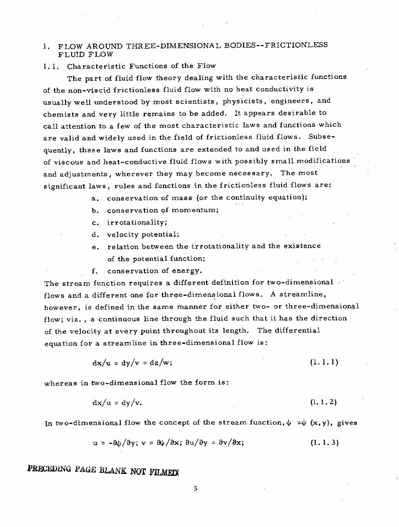
1. FLOW AROUND THREE-DIMENSIONAL BODIES--FRICTIONLESSFLUID FLOW
1. 1. Characteristic Functions of the Flow
The part of fluid flow theory dealing with the characteristic functions
of the non-viscid frictionless fluid flow with no heat conductivity is
usually well understood by most scientists, physicists, engineers, and
chemists and very little remains to be added. It appears desirable to
call attention to a few of the most characteristic laws and functions which
are valid and widely used in the field of frictionless fluid flows. Subse-
quently, these laws and functions are extended to and used in the field
of viscous and heat-conductive fluid flows with possibly small modifications
and adjustments, wherever they may become necessary. The most
significant laws, rules and functions in the frictionless fluid flows are:
a. conservation of mass (or the continuity equation);
b. conservation of momentum;
c. irrotationality;
d. velocity potential;
e. relation between the irrotationality and the existence
of the potential function;
f. conservation of energy.
The stream function requires a different definition for two-dimensional
flows and a different one for three-dimensional flows. A streamline,
however, is defined in the same manner for either two- or three-dimensional
flow; viz. , a continuous line through the fluid such that it has the direction
of the velocity at every point throughout its length. The differential
equation for a streamline in three-dimensional flow is:
dx/u = dy/v = dz/w; (1. 1. 1)
whereas in two-dimensional flow the form is:
dx/u = dy/v. (1.1. )
In two-dimensional flow the concept of the stream function, i =4 (x,y), gives
u = -ap/ay; v = al/ax; 8u/ay = av/x; (1.1.3)
PRECEDcING PAGE BLANK NOT FILME
3

and finally for the irrotational flow case:
aq /ax + 8/ay =v = 0, (1.1.4)
where the symbol v2 denotes the Laplace operator (Laplacian).
2. SOME CHARACTERISTIC FUNCTIONS FOR TWO- AND THREE-DIMENSIONAL FLOWS
2. 1. Stream Function in Two-Dimensional Flow
The stream function requires a different definition for two-
dimensional flow from that for three-dimensional flow. One of the most
useful definitions of the two-dimensional stream functions is that the
partial derivative of the stream function with respect to any direction is
the velocity component plus 90 degrees (counterclockwise) to the direction
of flow. (Streeter, p. 39). In addition it must satisfy the continuity equation.
The first part of Equation (1. 1.3), i. e. , u = .. . , v = ... , is true whether
the flow has rotation or not. For irrotational flow, however, the second
part of Equation (1. 1. 3) and Equation (1. 1. 4) are true. In particular,
Equation (1. 1. 4) shows that the stream function may be constructed as
the velocity potential for some other flow (Streeter, p. 39). Relations
between stream function, L5, and velocity potential, 4, are found by
equating the expressions for the velocity components:
a4/ax = a/ay; 84/ay = -a8i/ax. (2. 1. 1)
2. 2. Stream Function in Three-Dimensional Flow
Again, all of the details of three-dimensional flow will not be
presented, only those which may be pertinent to the specific problem of
the present report. The calculation of the stream function in three-
dimensional flow requires much more effort and energy than that for the
two-dimensional case. Of special interest and value is the Stokes'
stream function defined only for those three-dimensional flow cases which
have axial symmetry.
The above discussion demonstrates clearly the advantages of using
the two-dimensional flow representation over three-dimensional flow
representation, even in the cases where the actual flow in the physical
space is geometrically expressed as a space phenomenon. The following
representation of the flow phenomena in the viscous, incompressible
4

fluid in a three-dimensional space configuration will only use those
analytical methods which give the mathematical description in terms of
two independent variables.
3. FLOW PAST THREE-DIMENSIONAL BODIES IN VISCOUS
INCOMPRESSIBLE FLUID
3. 1. Flow Past a Circular Cylinder--Symmetrical Case
Flows past three-dimensional symmetrical bodies, in particular
flow past a circular cylinder in a symmetrical configuration, will be the
first case to be considered. The flow in the boundary layer past a
circular cylinder in the symmetrical case is known from the literature,
and the solution functions used here are taken from Schlichting, pp. 150-152.
The free stream velocity Uc is parallel to x-axis, and one begins with the
ideal velocity distribution in "potential" irrotational flow past a circular
cylinder of radius R and free stream velocity U.. In general, when one
considers the flow past a cylinder in the symmetrical case, one may use
the so-called Blasius series. According to Blasius, the potential flow
is given by the series:
U(x) = + u3x3 + u5x5 + u7x7 + u9x9 + u 1 1 x +...; (3. 1. 1)
where the coefficients u 2 , u 3 , ... , depend only upon the shape of the body
and are to be considered known. The pressure term in the boundary layer
can be easily calculated for the stationary condition and becomes:
- p- 1 dp/dx = U dU/dx; p = constant; (3.1, 2)
2 3 5 2U dU/dx = u x + 4 ulu 3 +x 5 (6 ulu 5 + 3 u 3 )
+ x7 (8 ul 7 + 8 u 3 u 5 ) + x 9 (10 U 9 + 10 u 3 u 7 + 5 u 5
+ x11 (12 uu 11 + 12 u 3 u 9 + 13 u 5 u 7 ) + ... ; (3.1.3)
where the continuity equation is integrated with the use of the stream
function 4 = (x,y). A suitable assumption for the coefficients of the
stream function and hence for the velocity components remains to be
made. For the general case, Blasius proposed the form for P(x,y), u
and v with the standard boundary condition (y = 0, u = v = 0, y = r,
5

u= Ua.
The case treated in this work refers to the boundary layer on a
cylindrical body placed in a stream which is perpendicular to its axis
(this axis will be denoted as the z-axis, perpendicular to the plane (x,y)
in which the flow actually takes place). Thus the flow is considered to
be two-dimensional in the (x,y) plane. In either case the velocity of the
potential flow is assumed to have the form of a power series in x, where
"x" denotes the distance from the stagnation point measured along the
contour of the cylinder. In the Blasius series, the velocity profile in
the boundary layer is also represented as a power-series in x, with the
coefficients assumed to be functions of the coordinate y, measured at
right angles to the wall; i. e., to the surface of the cylinder.
The form is:
U(x) = 2 UC sin = 2 Uc sin (x R1), (3.1.4)
and by expanding in a power series it becomes:
-1 1 -1 3 1 -1 5U(x) = 2 U [ (xR ) (x R ) + (x R
1 (x R-1)7 + ]; (3. 1.5)
the stream function with q = y R-1 (2 U -R -1 1/2 is:
= (vul 1/2 {ulx fl( ) + 4 u3x3 f3() + 6 u5x5 f5 (
+ 8 u 7 7 f7() + 10 u9x9 f9 (1) + 12 ulx
11 f1 1 (i) +
(3.1.6)
the functions u are:n
1 (U2 -3 2 -5u = (UR ; u5 UR ... ; (3. 1.7)
-1and the velocity u U 1 is given by:
-1 -1 4 -13 6 -15uU= 2 (xR ) f'1 ) (xR) f'3 + ) (xR) f'5
78 ( ) xR-17 f + . . (3.1.8)
where the functions f' are called the functional coefficients.n
6

In order to render the functional coefficients independent of the
particular properties of the profile, i. e. , of u l , u 3 , ... , it is necessary
to split them as follows ( for i > 5):
f'5 = g' 5 + (10/3) h' 5 ; (3.1. 9)
f7 = g' 7 + 7 h' 7 + (70/3) k' 7 ; (3.1. 10)
9 = g' 9 + 12 h' 9 + (126/5) k' 9 + 84 j' 9 + 280 q'9; (3. 1. 11)
f'll = g'll + (155/3) h'll + 66 k'll + 220 j' 1 + 462 qll " ; (3. 1. 12)
where all the functions shown are tabulated in Schlichting's work. The
usefulness of the Blasius' method is restricted by the fact that it should
not be used for slender bodies. Other attempts on the problem have been
made by Goldstein, Hiemanz, Goertler and others. For a circular
cylinder of diameter d = 9. 74 cm in a stream of velocity u = 19 cm sec - ,
Re = u d v = 1.85 x 10 , Hiemanz found that his experiment gave values
for u which could be represented sufficiently accurately by three terms
of the series for the potential flow. Due to the fact that the function f ( 1 )
are tabulated in Schlichting's work, this research will use the Schlichting
data throughout the report (see Schlichting, p. 152 to p. 154 after remodeling).
3. 2. Forms Used in the Analysis
Stream function
1/24 1 3
S(2 u U R) /2 {(R-x)f l() (R- x)3 f 3 (r)
6 -1 5 8 -17 10 1 9(R- x) f 5 (rj) - (R x) f 7 (r) +-0- (R- x) f
12 (R- x) 1 1 () + . . } . (3. 2. 1)
Velocity Components (Schlichting Data)
The velocity components are derived from the stream function:
u = (8 /y) = (8/8r) * (21/2 U/ Z R /2- 1/Z)
7

4 -13 6 -15= 2 U {(xR - )f 1(r) - (xR f + (x R- V (p)
8 (x R- 1 7 + (x R- 1 9 (7 99
S (x R- 11 + (3. 2. 2)
Similarly, the velocity component v is:
v= - aq/x ; (3. 2. 3)
v =- (2 v UR)1/2 {R- f1( ) - R- 3 x 2 f3(
+ R- 5 x 4 f5 () - R 7 X f)7(l) + L R- 9x8
12 R- 11 10 ) + . } = (2 U R -1 )1/2 .
(3. 2. 4)
In Schlichting's work one can find another form for the function v, (p. 149,
Equation(9. 20a))which, after inserting the corresponding values for the
coefficients un, is in perfect agreement with Equation (3. 2.4).
Final Forms of the Vorticity Component
8v/x = - (2 v U. R) 1 / 2 R- 2 {- (xR 1) f3
,120, -1 3 36 -1 )5+ (.) 0 )(xR- 3 5( ) - (6,) (xR- f(
720. i)7 1320 • 1)9+ (-. ) (x R- 7 fg9 () - ( )(xR- 1 f 1 1 (I) +
(3. 2.5)
(au/8y) = 2 U (2 R- 1 Um - 11/2 { (x R- ) f'1)
(xR- 1 3 (r) + ( ) (x R)
8 -1 7 10 -19-) (x R () + ( R) (x R- ()
12 - 11 f 1 ) + . } (3. 2. 6)) (x R fi 118
8

The function w in the formz
1 -1 (3.2.7)S=- [( 0 v/ax) - au/8y)], = sec ,
will be superimposed upon each curve u Uc0 - to illustrate the perturbed
velocity distribution in the laminar boundary layer on a circular cylinder
at the following set of angles:
= 00; =200; =400; =600; = 800; = 900; = 1000; = 1100. (3. 2. 8)
where c = (x R -1
4. PERTURBATIONS
4. 1. Stream Function
Thus, there have been derived the equations for the stream function,
S= %(x,I) = 4i(x,.T (y)), and the equations for the velocity components,
(u,v), in the specific flow in question, i.e. , the symmetrical case of
the flow past a circular cylinder (Blasius series). From the definition
of the stream function one can derive the equation of the streamlines.
Since, the stream function satisfies the equation of continuity, the curves,
t5 = constant, represent streamlines (Owczarek, p. 63). The research
begins with the stream function (see Equations (3.2. 1) and (3.2.4) above):
1/2 -l 4 -13= (2 v U, R) {(R x)f()f (- (R x) f3 (r )6 - 5 8 - )7 !0
+ 6( f5 -71 (R- x) 7 -+ (R -x) 9 f (T
_ 1 (R- x) 1 l11 ( + . } = constant. (4.1.1)
Put in this form, the function j is a function of two variables, (x, r), or
(x,), x = x R - 1 (dimensionless), or (x,y), since q = constant y, where
the constant is a dimensional number. Thus, both the coordinates
(x,ri) appearing in the representation of the function 4, Equation (4. 1. 1)1/2
are dimensionless, and only the coefficient (2 v U R) standing in2 -1front of { ... has the dimensions of cm sec as it should be. The
part of the stream function in the braces, { . .. ) , must be kept constant
in order that the stream function be constant (condition for the streamlines).
In other words, the condition for streamlines appears in the form:
9

4 136 =1x3x)5 f(R -x) f ( (R x) ) + (R x) f 5 ()
8 (R-1 )7, (R1x) 7 () + .. = constant; (4. 1.2)
and one may group the above terms in the following manner:
-1) 16 (R-1x)5 15S(R ) fl (R 7 )) 7
[ ()] (R x)3 f3()] + (Rx)' 11 f()]
8[ ,R-I )7 f7 (ij)] + [! -. (R-l )9 fg ()] -[12 (R )11
= constant = C. (4. 1. 3)
Obviously, there are infinitely many possibilities for dividing the constant
appearing on the right hand side of Equation (4. 1. 3) among the infinitely
many terms of the series appearing on the left hand side of the same
equation. For illustrative purposes, the following scheme is proposed:
the constant C is divided into "m" equal parts, where "m" is equal to
the number of terms on the left hand side of (4.1.3); each term is assumed
to be equal to Cm ; and (R ) :
f -1x fl( ) = Cm ;
4 3 -1(x) f3(T) Cm
)5 5() = C m-1 (4. 1.4)
8 - -1- ()5 f (7) Cm7- - () 7 f 7 () -Cm
10 9 -1-97. (X) fg( ) = Cm ;
and so on
although there may be other alternatives, one of the conclusions of the
system of equations, (4. 1. 4), is that, in the first form of (4. 1. 4), both
the variables, (x,rT), or any logical combination of these variables such
as the product or the ratio are assumed to be constant. Again from the
many possible combinations, which may and probably do occur in the
actual, physical conditions, the following combination are selected for
10

purely illustrative purposes:
x = constant = C A , (4. 1. 5)
[ ()nl] = constant; 1 = y R -1(2 UmRi 1 1/2 (4. 1.6)
The first possibility, Equation (4. 1. 5), will be discussed in more detail.
As can be seen from Equation (4. 1. 5) this is an equation of a hyperbola.
Consequently, in the case under consideration, the simplest possible
geometrical form of a streamline in the (x,y) space is a hyperbola,
Equation (4. 1. 5).
4. 2. Elementary Geometrical Characteristics of the Hyperbola
The geometrical characteristic of hyperbola are collected and presented
in orcter to use them in the present work, thus eliminating the need for
outside references. The standard form of a hyperbola is:
2 -2 2 -2 (4. . )x a -y b =; (4.2.1)
where the axis, x, intersects the hyperbola at the vertices A and A ;
the segment Al .- A2 is the transverse axis; both branches of hyperbola
are symmetrical with respect to (A 1 AZ), one part being below and another
above the axis; the y axis does not intersect the hyperbola since the center
of the coordinates (x,y) is located in the center between Al and A 2 .
From Equation (4. 2. 1), if a = b, the hyperbola is equilateral, and if the
asymptotes are perpendicular to each other, the hyperbola is "rectangular."
The equation of a rectangular hyperbola in which its asymptotes are
referred to as coordinate axes is:
x 1 =, (4. 2. 2)
2 2a =b =A ,
and is located in the first and third quandrants. For such a hyperbola12 12
one has x y = a (first and third quadrants), = a (second and
fourth quandrants);
semi-axes: a = b = (2A)1/2 ; (4. 2. 3)
c 2 4A; c =ZAl/2; (4.2.4)
11

coordinates of foci: (-ZA / , 0) (2A1/2, 0); (4. 2. 5)
coordinates of vertices: [(-2A)1/2 , 0] ; [(2A)1/2, 0] ; (4. 2. 6)
eccentricity: e = c a-1 = 1/2 ; (4. 2.7)
distance of the center to directrix: a e-1 = A ; (4. 2. 8)
equation of directrices: x = A1/2, or x = -A1/2 ; (4.2.9)
equation of the asymptotes: x - y = 0, x + y = 0; or x = y, x = -y (4. 2.10)
Consequently, equation (4. 1.5) is the equation of a rectangular hyperbola
in which its asymptotes are referred to as dimensionless coordinate
axes (R-Ix, -) or (x, i). This coordinate system will be used as the
basic coordinate system in further considerations, discussions and
plotting of the diagrams.
4. 3. Computer Plots
The plots, included in the present report refer to a solution of the
steady-state boundary layer equation in the flow past a circular cylinder
in the symmetrical case (Blasius series). In particular the plots refer-1
to the horizontal velocity component in the case given by u U_1 as quoted
previously:
-1 4 -3u U = 2 {x f'1 ) = (x)3 f,3 (r) + .} (4.3. 1)
-1The plots of the function of u U 1 as a function of two variables are given
-1in the Schlichting book (p. 153) where the function u U,~ is a function of
y R1 (U R = ( 1/2 21/) and of = xR1, with 4 being treated as a
parameter in the range of = 00 , 200, 400, 600, 800, 900, 1000, 108. 80.
Similar plots have been accomplished from this research which are done
automatically in their entirety from the output plotter as part of the
CDC 650 Computer System. These plots are functions of the independent
variable T] varying from r~ = 0 up to 9 = 4. 0, and for the values of the
parameter c, c = x R I
= 100, 200, 300, 400, 500, 600, 700, 800, 900, 1000, 1100
Since this effort deals with the problem of the flow in a viscous
12

fluid (viscosity is defined as a transverse transfer of momentum) any
possibility of obtaining a purely theoretical laminar flow around a
cylinder is automatically excluded. One can only talk about a quasi-
linear flow or a flow with small disturbances due to small viscosity
pheomena. In order to make the disturbances due to viscosity visibly
more observable, the concept of disturbance in the form of the vorticity
function, wt, containing (8v/8x), and (8u/8y), has been introduced whichz -1
is then superimposed upon the velocity function, u U, . This is done
geometrically, by means of plotting the diagrams of (u U I ) as the
function of 1 in the two-dimensional Cartesian coordinate system,
(u U.1) and q = y R- (2 U R-1 1/2, with =x = (x R1) being a
parameter, and R being a fixed constant. Moreover, the function wz
is also plotted in the same diagram and in the same coordinate system
as a function of rI. Under the assumption that one is dealing with the
linear Schroedinger equation as the basic equation, the principle of
superposition can be applied and the values of the two functions u U l
and wz , and be added geometrically for each value of the independent
variable, r~. The final operation can then be performed for obtaining
the sum of functions. This technique has been applied and the resulting
plots are included as Appendix A of the report. It is not essentialwhich
coordinates in all of the systems discussed be chosen: (x,y) or (x,y),
(x, j), (x, T), since obviously the coordinates x and x, y and 'i differ
only by constants, one being dimensional and the other dimensionless,
respectively. In conclusion, one may summarize the results obtained
as follows:
(a) the stream function of the flow around a circular cylinder,
located symmetrically, is given by Equation (4. 1. 1);
(b) the velocity component u is given by Equation (3. 2. 2);
(c) the velocity component v is given by Equation (3. 2. 4);
(d) the disturbance function (in form of the curl of velocity) is
given by Equations (3. 2. 5), (3. 2. 6), and (3. 2. 7); this is
(geometrically) superimposed upon the velocity component-1
function u U-
(e) the condition for the streamlines is given by Equation (4. 1. 3);
(f) the simplest possible geometrical form of a streamline in
the (x,y) or (x, q) space is the hyperbola (xq) = CA;
13

(g) consequently, the result of the case of flow around a circular
cylinder is exactly the same as in the previous case of the
laminar flow along an infinitely long plate. A finite but very
small amount of vorticity introduced into the flow system
causes the appearance of small disturbances. These disturbances
originate at each finite element and spread in the fluid for short
distances. In the case of the flat plate the streamlines were
parabolas whereas in the present case they are hyperbolas
as proven in Equation (4. 1. 5).
As in the case of a flat plate, one assumes a moving coordinate
system (x,y) or rather [ (x R-l),q] along each of the curves given as the
sum of [(u U ) + Wz ] , from Equation (3. 2. 2), plus Equation (3. 2. 7) with
Equations (3. 2. 5) and (3. 2. 6), supplying a series of values of the para-
meter xR- 1 = = 00, 200, ... , 1100. Each chosen point for a certain
value of i is assumed to be the vertex of the rectangular hyperbola.
The moving coordinate system moves parallel to itself and to the fixed
coordinate system, [ (xR-1), vertical axis] . The branches of the hyperbola
are located in the first and third guadrants. From both coordinate axes,
the horizontal axis (R - 1 x) is always horizontal and the other axis is
always vertical. By means of the proper transformation (of coordinates
if necessary) the branch of hyperbola located in the third quadrant is
being shifted along the transverse axis (A 1 - A 2 ) so that both vertexes
A1 and A 2 coincide at the vertex of the branch of the hyperbola located
in the first quadrant. Consequently, the first quadrant branch of hyperbola
is oriented from up-down and to the right; the third quadrant branch of
hyperbola is oriented from down-up and to the left; both branches meet
at their vertexes (A at the same point as A2 ) and both vertexes coincide
with the point chosen on the curve [ (u U ) + wz]. The two branched hyperbolas-1
in question are traced at a number of points along the curves [ (u UM ) + Wz]
and their points of intersections are located. The sections of streamlines
(hyperbolas) between two found points of intersection furnish the zig-zag
pattern of the path of a particle. This produces the resulting pattern of
disturbances in the flow around a circular cylinder caused by the injection
of the vorticity geometry into the regular pattern. These zig-zag patterns
are traced in a few cases. The data used in the computer plots are the same
referred to previously:
14

-1 -1Ua, = 200 km hour = 5555. 55 cm sec ;
2 -1v = 0. 149 cm sec .
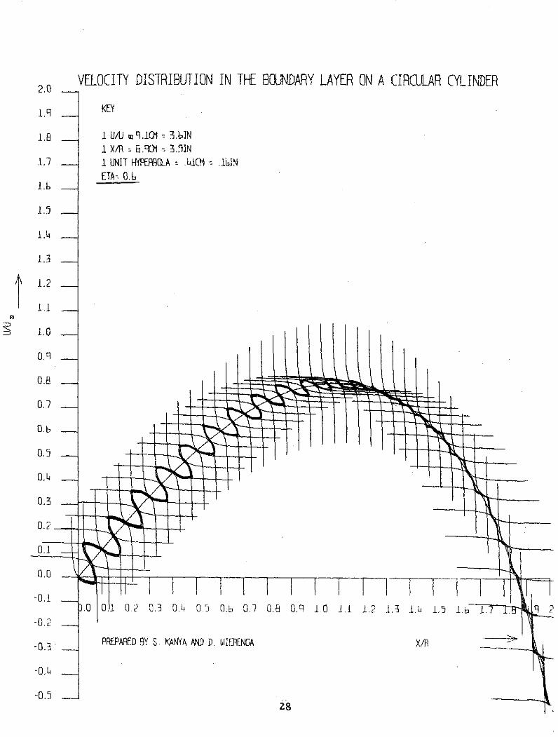
4. 4. The Plots
The first set of plots .refers to the flow around a circular cylinder-1
in the symmetrical case. The velocity distribution, (u U_ ), is taken
as a function of (x R - 1) for various values of the coordinate 1, considered
to be a parameter. The value of q for 20 values is taken to be ( -
yR " I (ZURv ) 1/ 2
S=.0. 2, 0.4, 0. 6, ... ,...., 3. 8 = 4. 0; (4.4.1)
In this approach no disturbances are superimposed upon the flow. The
20 plots included at the end of the present report are based on the values-1
of the function of (u U 1) as taken from Equation (3. 1. 8) or (4. 3. 1).
For a certain number of points of these functions the streamlines are
plotted as double-branched hyperbolas, and the points of intersections
of these hyperbolas are found; the sections of streamlines between the
points of intersection are interconnected thereby displaying the zig-zag
pattern as the path of a particle. The results show that the zig-zag
pattern, which indicates the existence of some disturbances in the boundary
layer, appears even in the flow without the introduction of any outside
disturbance such as vorticity. This can be expected in this kind of flow.
It seems desirable to point out that one may question the accuracy and
the precision of the graphical results and of the plots in the neighborhood
of x R-1 equal to 2. 0. This may be partly justified since it must be kept
in mind that: (a) the present calculations were done primarily for
illustrative purposes, and for providing general conclusions giving
insight into the particular points and pecularities of the problem needing-1
more emphasis, and (b) the point in question (R - x = 2) lies outside the
region of the separation of the flow and consequently the characteristic
properties of the flow at this particular point cannot be measured with
precision.-1
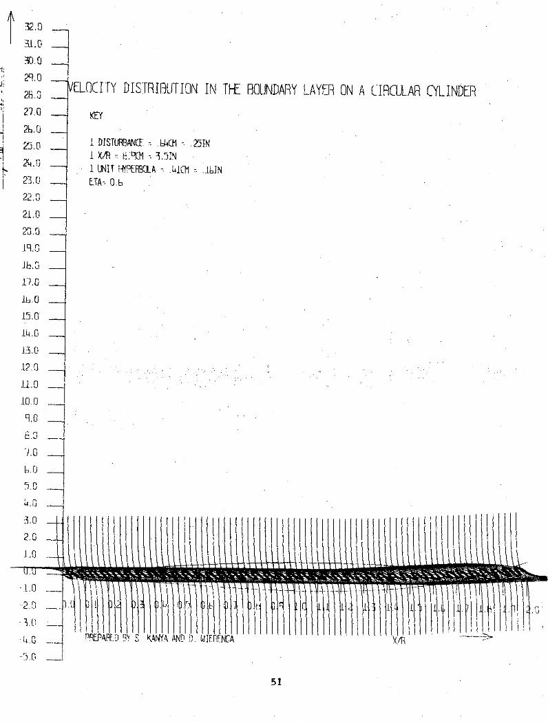
The second set of plots is based on the curve u U. 1 plus a disturbance
with resultant curve:
u U+ = resultant curve; (4. 4. 2)
15

on each curve (u U 1 ) taken from the first set of plots there is super-
imposed the disturbance curve in the form of wz as the function of 9.
Each graph therefore clearly shows two curves: one describing the value
of u U. 1 as the function of ii and the second curve describing the vorticity
function, w , again as the function of r1. The vertical coordinates on
these two curves are geometrically added giving the resultant curve,
Equation (4. 4. 2). Again at a certain number of points on this curve,
the two-branched hyperbolas are plotted and the points of intersections
of the streamlines (i. e. , of hyperbolas) are located. The zig-zag
patterns of the paths of particles are traced thus giving the final results.
The third set of plots refers to the velocity vd (dimensionless) =
v U-1, Equation (3. 2. 4), which is subject to disturbances in the form of
the vorticity, toz , i.e.:
vd = v U;-1 v from Equation (3. 2. 4); vd + Wz = resultant function
(4.4.3)
Again, at a certain number of points of the curve (vd + Wz) two-branched
hyperbolas are plotted, the points of intersections of the streamlines
(i. e. , of hyperbolas) are located, and the zig-zag patterns of the paths
of particles are traced, thus giving the final pattern.
All the plots described above and included in this report demonstrate
the existence of the zig-zag patterns in the flow in question, regardless
of whether the flow is laminar, irrotational, rotational, or there is or
is not a vorticity function geometrically superimposed upon the velocity
functions of u and v components. The existence of the zig-zag pattern
is proof that the flow is not laminar, the particle paths are not parallel
(nor quasi-parallel) lines. This is an obvious indication that there are
disturbances in the particular flow in question due to the shape (circular)
of the body around which the flow takes place. The laminar flow along a
flat plate demonstrates the zig-zag pattern. There does not exist a
laminar flow in a domain of a viscous, heat-conducting fluid flow (above
the X-transition point). This conclusion, which is in accordance with
Heisenberg's statement, has been discussed in previous reports. The justi-
fication for the use of summation law, association between the wave mechanics
and deterministic macroscopic fluid dynamics, and all the other aspects are
also explained in previous reports.
16

5. FINAL REMARKS
A comparison of the geometry of the flow patterns of the laminar
flow past a symmetrically located cylinder (Schlichting, pp. 146-155) and
those in Technical Report No. 3 indicates a few important results:
(1) The so-called "laminar" flow around a cylinder (symmetri-
cal case or not) is not a laminar but is a flow with disturbances;
(2) Disturbances are always present in the so-called "laminar"
flow due to the transverse transfer of momentum (viscosity);
(3) The zig-zag paths appear always in the so-called "laminar"
flow, however small they may be since streamlines are
always there;
(4) The "streamlines" in the "laminar" flow are actually the
mean value paths of the real zig-zag paths of the particles;
due to the fact that zig-zag paths are small (small amplitudes)
and due to the physiological aspects they are seen by the
naked human eye as continuous lines (the streamlines);
(5) The above traced zig-zag paths seem to be very "regular"
whereas the oscillograms obtained from the oscillographs
placed in a turbulent jet (see Technical Reports No. 1 and 2)
demonstrate that often the realistic zig-zag paths are
irregular; a certain regularity in zig-zag paths may or may
not appear in the "periodic" sense. This demonstrates that
"local' irregularities (jumps, sharp steep "mountains",
sharp, steep "valleys") have their origins and are due to
other reasons and phenomena not yet discussed (interference,
inter -correlation);
(6) When the zig-zag paths are very "even", regular and of small
amplitudes, a zig-zag path may be seen by the naked human
eye as one thick "streamline", as one thick ray; a light, a
ray of light, which is also a wave;
(7) The problem of interference and inter-correlation is discussed
in Technical Report No. 1.
17

REFERENCES
Abell, B. F. , The Invisible C. A. T. , Aerospace Bulletin, Parks Collegeof Aeronautical Technology, St. Louis University, Vol. V, No.1, Fall 1969.
Abrikosov, A. A., Gordv,. L. P. , and Dzyaloshinski, I. E., translated
by R. A. Silverman, Methods of Quantum Field Theory inStatistical Physics, Prentice-Hall, Inc., 1963.
Batchelor, G. K. , The Theory of Homogeneous Turbulence, CambridgeUniversity Press, 1953.
Baym, G., Lectures on Quantum Mechanics, W. A. Benjamin, Inc.,196.9.
Bird, R. B. , Stewart, W. E., and Lightfoot, E. N., TransportPhenomena, John Wiley and Sons, Inc. , 1967.
Blasius, H., Grenzschichtenin Fluessigkeiten mit kleiner Reibung,Z. Math. u. Physik, 56, 1, 1908.
Bohm, D., A Suggested Interpretation of the Quantum Theory in Termsof "Hidden" Variables, I, II, Physical Review, Vol. 85, No. 2,January 15, 1952, pp. 166-193.
Bohm, D., Quantum Theory, Prentice.Hall, Englewood Cliffs, N. J. ,1951, 1964.
Brodkey, S. R., The Phenomena of Fluid Motions, Addison-WesleyPub. Comp. , U. S. A., 1967.
Burgers, J. M., A Mathematical Model Illustrating the Theory of Turbulence,Adv. in Appl. Mech. , Vol. 1, 1948, Academic Press, N. Y.,pp. 171- 199.
Chapman, S. , and Cowling, T. G. , The Mathematical Theory of Non-Uniform Gases, Cambridge University Press, London, 1952.
DeWitt, B. S., Quantum Mechanics and Reality, Physics Today, Vol. 23,No. 9, September 1970, pp. 30-35.
Dryden, H. L., The Turbulence Problem Today, Proc. of the FirstMidwestern Conference on Fluid Mechanics, J. W. Edwards,Ann Arbor, Michigan, 1951, pp. 1-20.
Dryden, H. L., Boundary Layer Flow Near Flat Plates, Proceed. 1stInternat. Congress for Appl. Mechanics, Delft, 1924,pp. 113- 128.Also Proceed. 4th Inter. Congress for Appl. Mech., Cambridge,
1934, pp. 175. Also NACA, Report No. 562, 1936 (see especiallyFigure 17). Also Journal of the Washington Academy of Science,25, (1935), 106.
fXEcDNG PAGE BLANK NOT FILMI19

Dryden, H. L., Recent Advances in the Mechanics of Boundary LayerFlow, Adv. in Appl. Mech., Vol. I, Acad. Press, Inc., New York,1948, pp. 1-40.
Fage, A., The airflow around a circular cylinder in the region wherethe boundary separates from the surface, Phil. Mag. 7, 253,1929. Also A. R. C. Reports and Memoranda, No. 1580; 1934,pp. 1-7.
Fluegge, S. , Practical Quantum Mechanics, I and II, Springer- Verlag,New York, Inc., 1971.
Fuller, G., Analytic Geometry, Addison-Wesley Publ. Company, 1967.
Glauert, H., The Elements of Aerofoil and Airscrew Theory, Cambirdgeat the University Press, 1937.
Goertler, H. , A New Series for the Calculation of Steady Laminar BoundaryLayer Flows, Journal of Mathematics and Mechanics, Vol. 6,No. 1, 1957, pp. 1 to 66.
Goldstein, S. , Modern Developments in Fluid Dynamics, Vol. I and II,Oxford at the Clarendon Press, 1938.
Grad, H. , Kinetic Theory and Statistical Mechanics, Lectures, NewYork University, 1950.
Green, H. S., The Molecular Theory of Fluids, North-Holland Publish.Comp. , Amsterdam, 1952.
Hansen, M., Die Geschwindigkeitsverteilung in der Grenzschicht an einereingetauchten Platte, ZAMM, 8, 1928, p. 185.
Hinze, J. O., Turbulence, McGraw-Hill Book Company, Inc. , NewYork, 1950.
Hirschfelder, J. O. , Curtiss, C. F. , and Bird, R. B. , MolecularTheory of Gases and Liquids, John Wiley and Sons, 1954.
Hovanessian, S. A., and Pipes, L. A., Digital Computer Methods inEngineering, McGraw-Hill Book Company, New York, 1969.
Howarth, L. , On the Solution of the Laminar Boundary Layer Equations,Proceedings Royal Soc. London, A164, p. 547, 1938.
Howarth, L., Modern Developments in Fluid Dynamics, High SpeedFlow, Vol. I and II. Oxford at the Clarendon Press, 1953.
Jeans, Sir James, An Introduction to the Kinetic Theory of Gases,Cambridge University Press, 1940.
Kennard, E. H., Kinetic Theory of Gases, McGraw-Hill Book Company,New York, 1938.
20

Krzywoblocki, v. M. Z., On Some Aspects of Diabatic Flow and GeneralInterpretation of the Wave Mechanics Fundamental Equation,Acta Physica Austriaca, Vol. XII, No. 1, 1958, pp. 60-69.
Liepmann, H. W. , and Puckett, A. E. , Aerodynamics of a CompressibleFluid, John Wiley and Sons, Inc. , New York, 1947.
Lindsay, R. B., General Physics, John Wiley and Sons, Inc., 1947.
Loeb, L. B., The Kinetic Theory of Gases, McGraw-Hill Book Company,New York, 1934.
Madelung, E. , Quanthentheorie in Hydrodynamischer Form, Zeitschriftfuer Physik, Vol. 40, 1926, pp. 322-325.
Milne, E. A. , The Tensor Form of the Equations of Viscous Motion,Proceedings, Cambridge Philosophical Soc., Vol. 20, 1920-21,
pp. 344-346.
Mises, von T., Mathematical Theory of Compressible Fluid Flow,Academic Press, New York, 1958.
Neumann, v. , Johann, Mathematische Grundlagen der Quantenmechanik,Springer-Verlag, 1932, 1968.
Neumann, v. Johann, translated by R. T. Beyer, Mathematical Foundationsof Quantum Mechanics, Princeton University Press, 1955.
Owczarek, J. , Fundamentals of Gasdynamics, International TextbookCompany, 1964.
Pai, S. I. , Viscous Flow Theory, I. Laminar Flow, D. Van NostrandCompany, Inc. , New York, London, 1956. II. Turbulent Flow,Ibid, 1957.
Pao, R. H. F., Fluid Dynamics, Charles E. Merrill Books, Inc., 1967.
Patterson, G. N., Molecular Flow of Gases, John Wiley and Sons,New York and London, 1956.
Peierls, R. E. , Quantum Theory of Solids, Oxford University Press,New York, 1955.
Pohlhausen, E. , Der Waermeaustausch Zwischen Festen Koerpern undFluessigkeiten mit Kleiner Reibung und Kleiner Waermeleitung,ZAMM, 1, 115, 1921.
Prager, W. , Introduction of Mechanics of Continua, Ginn and Company,1961.
Prandtl, L. , Veber Fluessigkeitsbewegung mit sehr kleiner Reibung,Proceedings 3rd Intern. Math. Congress, Heidelberg, 1904.
Reprinted in "Vier Abhandlungen Zur Hydrodynamik und Aerodynamik,Goettingen, 1927; also: NACA, TM452 (1928).
21
Prandtl, L. , and Tietjens, O. G. , translated by J. P. Den Hartog,Applied Hydro and Aeromechanics, McGraw-Hill Book Company,Inc. , New York and London, 1934.
Reynolds, O. , An Experimental Investigation of the Circumstances whichDetermine Whether the Motion of Water Shall be Direct or Sinuousand of the Law of Resistance in Parallel Channels, Trans. Roy. Soc.(London), A174, 1883, pp. 935-982; Sc. Paper 2:51.
Samaras, D. G., The Theory of Ion Flow Dynamics, Prentice Hall, Inc.,Englewood Cliffs, N. J. , 1962.
Schlichting, H., translated by J. Kestin, Boundary Layer Theory, McGraw-Hill Book Comp. , Inc. , New York and London, 1960.
Schmidt, E., translated by J. Kestin, Thermodynamics, ClarendonPress, Oxford, 1949.
Schroedinger, E. , Wellen -Mechanik, Ann. d. Phys. 79, p. 361, 489.80, p. 437; 81, p. 109, 1926.
Shkarofsky, I. P. , Johnston, T. W. , and Bachynski, M. P. , The ParticleKinetics of Plasmas, Addison-Wesley Publishing Company, Inc.,Reading, Mass., London, 1966.
Stewart, O. M., Physics, Ginn and Company, Boston-New York, 1944,
Streeter, V. L., Fluid Dynamics, McGraw-Hill Book Company, Inc.,1948.
Taylor, G. I. , The Statistical Theory of Turbulence, Part I-IV, Proc.Roy. Soc. (London), A151, 1935, p. 421.
Theodorsen, T., The Structure of Turbulence, (see J. B. Diaz and S. I.Pai, Fluid Dynamics and Applied Mathematics), Gordon andBreach, 1962.
Truesdell, C. , The Kinematics of Vorticity, Indiana University Press,Bloomington, Indiana, 1954.
Van der Hegge Zijnen, B. G. , Measurements of the Velocity Distributionin the Boundary Layer Along a Plane Surface, Thesis, Delft, 1924.Also see Proceed. 1st Intern. Congress for Applied Mechanics,Delft, 1924, pp. 113-128.
Vazsonyi, A. , On Rotational Gas Flow, Quarterly of Applied Mathematics,Vol. III, 1945, No. 1, pp. 29-37.
Wehrmann, O. , Quantum Theoretic Methods of Statistical Physics Appliedto Macroscopic Turbulence, Vereinigte Flugtechnische Werke-Fokker, Bremen 1, West Germany (private communication).
Weinberger, H. F. , Partial Differential Equations, Blaisdell PublishingCompany, New York, Toronto, London, 1965.
22

The First Set of Plots
The function (u U ) as the function of (x R ) for various
values of the parameter r = 0. 2, 0.4, ... , 4. 0.
No disturbances.
23

2.0 VELOCITY DISTRIBUTION IN THE BOUNDARY LAYER ON A CIRCULAR CYLINDER
1.9 I KEY
1. I U/U m 9.1CM - .biN iI X/R B.CM = 3.5IN
1.7
1.5
1.3
1.21.1
1.0
0.9
0.2
0.'7
0.0
0.1
0 0.1 0.2 0. 0.lw l. 5 0.b 0.7 0.0 0. 1 0 1 1 1.2 1.3 1.4 1.5 1.b 1.7 1.8 9 2.0
-0.3 PREPARD BY S. KANYA AND D. WIEP NGA X/R
0.~FRE EPING PAGE BLANK NOT FILMED
25

2.0 VELOCITY DISTRIBUTION IN THE BOUNDARY LAYER ON A CIRCULAR CYLINDER
1.9 KEY
1.8 1 U/U m q.11 - 3.biN1 X/R B.qCM 3..IN
1.7 1 UNIT HYPERBOLA .UCM J. blNETA= 0.2
1.
1.5
1.4
1.3
1.2
0.8
0.7
0.b
0.5
0.3
0.2
0.1
0.0
.0 0.1 0.2 0.3 04 0.5 I 0 G i O 1 0 1 1 1" 1.3 1.1 1 5 lb 17 18 1 9 2 00.2
0.3 PREPARED 9Y S KANYA AND D WIERENGA X/R
0.4
-0.5
26

2.0 VELOCITY DISTRIBUTION IN THE BOUNDARY LAYER ON A CIRCULAR CYLINDER
1.9 KEY
1.8 1 U/U m 9.1CM - 3.bINI X/R = B.9CM -. 5IN
1.7 1 UNIT HYPERBOLA - .b1CM -= .1lN
ETA= 0.'
1.5
1,.4
1.3
1.2
1.1
1.0
0.8
0.7
0.b
0.5
0.4
0.3
0.2
0.0 -
.0 0.1 0.2 03 0. 0.' 0.b 0.7 0.8 0. 1.0 1.1 1.2 1.3 1.b 1.5 1b 1.7 1. 9
0.3 PREPARED BY S. KANYA AND D. WIERENGA X/R
0.
-0.527
2.0 VELOCITY DISTRIBUTION IN THE BOUNDARY LAYER ON A CIRCULAR CYLINDER
1.9 KEY
1.8 1 U/U m 9.CM 1 3.bIN
I X/R 1= B. M 13.5IN1.7 1 UNIT HYPERBOLA .lCM .1blN
ETA= 0.b1.6
1.5
1.5
1.3
1 .2I.1.0
0.q
0.8
0.3
0.3
0.2
0.1
0.0
-0.1.0 0.1 0..2 0.3 , 1.1 1. 1.- 0H 1.5 ..1-1 1 2 1-3 ,9 2
-0. PREPARED 9RY S. KANYA AND D. WIERENQA X/R
-0.4
-0.518

2.0 VELOCITY DISTRIBUTION IN THE BOUNDARY LAYER ON A CIRCULAR CYLINDER
1.9 KEY
1.8 1 U/A m 9.101 --3.bINI X/R B.CMl =- 3.5IN
1.7 1 UNIT HYPERBOLA - .4lCM .[blNETA- 0.8
l.5
1.
1.3
1.2
1.0
0.8
0.7
O.6
0.5
0.3
.--40.2
0.0
-0.1.0 0.1 0.2 0.3 0.6 0.5 O.b 0.7 0.6 O.q 1.0 1.1 1.2 1.3 1.L 1.5 l.b 1.7 16 1.9 2 0
0.2 "
0.3REPARFD 9Y S KANYA AND D. WJIEJENGA X/R0.3
0.529

2.0 VELOCITY DISTRIUTION IN THE BOUNDARY LAYER ON A CIRCULAR CYLINDER
1.9 KEY
1.8 I U/U m .101CM 3.bINI X/R 7: .9Q01 =3.1IN
1.7 1I UNIT HYPERBOLA .hl4CM .1blN
ETA- 1.01.b
1.5
1.4
1.3
1.2-
1.0
0.9
0.6
0.7
0.b
0.5
0.3
0.2
0 .0 -
-0.1 T.0 0.1 0.2 0.3 0.1 0.5 0.b 0.7 0.8 O.q 1.0 1.1 1.2 1.3 1. 1.5 1.b 1 7 1.8 1.9 2
-0.2
*0.4
0.5
30

VELOCITY DISTRIBUTION IN THE BOUNDARY LAYER ON A CIRCULAR CYLINDER2.0
1.9 ' KEY
1.8 1 U/U m 9.11 = 3.bIN1 X/R .CM 3.51N
1.7 1 UNIT HYPERBOLA ,LICM .IlblN
ETA- 1.21.b
1.5
1.3
1.0
0.90.b
0.6
0.3
0
0.0
-0.1. 0.1 0.2 0.3 0. 0. 01, 0.0.7 0. 0.9 1.0 1.1 1.2 1.3 1.1 1.5 1.b 1.7 1. 1.9 2.
0.2
PREPARED BY S. KANYA AND D. WIERENGA X/R
-0331

2.0 VELOCITY DISTRIBUTION IN THE BOUINDARY LAYR ON A CIRCULAR CYLINDER2.0
1.9 KEY
1.8 I U/U m 9.1CM 3.bIN1 X/R - .'11 3 .51N
.1.7 1 UNIT HYPERBOLA -- .ICM .1blN
ETA: 1. 4
1.5
1.14
.1 3
1.0
0.9
0.8
0.)
0.b
0.5
0.'
0.3
0.0
__
.0.1.0 0.1 0.2 0.3 0. 0. 0.b 0.7 0.8 1 0 1.1 1.2 13 1.' 15 i b 1.7 1. 1.9 2.0
-0.2
-0.3 PREPARED 8Y S. KANYA AND D. WIERENGA X/n
0.34
o.5 _2

2.0 VELOCITY DISTRIBUTION IN THE BOUNDARY LAYER ON A CIRCULAR CYLINDER
1.9 _ KEY
1. __ I U/U m 9.1K 3.bINI X/R -B.C - 3.51N
1.7 I UNIT HYPERBOLA .41CM - .16NETA: 1.L
1.b
1.1
1.0
0.8
0.7
O.b
0.5
0.
0.3
0.
0.0
00.1 0.2 0.3 0. 0.5 0.C 0.7 0.8 I. 1.0 1,1 1.2 1. .i.U .1.5 1,b .1 7 1.B ~1 2.0
-0.2
03 PREPARED BY S. KANYA AND D. WIERENGA X/R
-0.3
.0.533

2.0 VELOCITY DISTRIBUTION IN THE BOUNDARY LAYER ON A CIRCULAR CYLINDER
1.9 KEY
1.8 1 U/U m9.CM 3.bINI X/R = 8.9 = 3.51N
1.7 1 UNIT HYPERBCLA - .h1CM .16blN
ETA .1.81.
15
1.3
t 1.2
0. 10.9
0.7
0.b
0.5
0.b
0.3-
0.0
--0.11.0 0.1 0.2 0.3 0.( 0.5 0. 0. .0 . .O 1.1 12 1.3 .Li I.b i.7 1.8 1. 2.!
0.2
-0.3 DPAREDPAR. BYS S KANYA AND D. WIRFNGA X.,/
0.34
0.534

2.0 VELOCITY DISTRIBUTION IN THE BOUNDARY LAYER ON A CIRCULAR CYLINDER
1.q 9 KEY
l.B 1 U/U m .11CM 3.bl6N1 X/R - B.CM = 3.51N
1.7 1 I UNIT -HYPERB_ A .h1CM - .1 blNETA- 2.0
1.b
1.5
I U
1.3
1.0
0.7
0.1
0.3
.0 0.1 0.2 0.3 0.4 0.5 0.b 0.7 0.6 0.9 1.0 1.1 1.2 1.3 1.u 1.5 1lb 1 7 1. 1.9 2.-0.2
-0.3 PREPARED BY S. KANYA AND D. WIERENGA X/R-0.3
-0.535

VELOCITY DISTRIBUTION IN THE BOUNDARY LAYER ON A IRCULAR CYLINDER2.0
1.9 KEY
1.8 1 U/U m .ICM - 3.b1NI X/R .B M - -.IN
1.7 i UNIT HYPERBOLA - .ulCM . IN
ETA, 2.21.b
1.5
1.2
1.1
0.9
0.6
0.5
0.3
0. 2.
0.0 71 -II --- i -
-.0 0.1 0.2 0.3 0., 0.5 0.b 0.7 3 . O.q .O I 10. 113 1. 1. 5 .U .i 1.7 1I6 i.q 2.
-0.2
_-0.3 PREPARED BY S. KANYA AND D. WIERENGA X/R
0.
-0.536

VELOCITY DISTRIBUTION IN THE BOUNDARY LAYER II C1 R CYLINDER2.0
1.9 KY
1.B I U/U m 9.IM 3.bINI X/R -- E.Q 3.5IN
1.7 _ I UNIT HYPERBOLA U .blCM .61INETA: 2.4
1.5
1.3
q 1.2
1.1
1.0
0.'
0.7
O.k
0.5
03
0.3
0.0 I I1
0.1.0 0.1 0.2 0.3 0.6 0.5 0.6 0.7 0.6 0.9 1.0 1.1 1.2 1.3 1. 1.5 1.6 1.7 1.~ 1.9 2.0
0.2
PREPARED BY S. KANYA AND D. WIERENGA X/R-0.3
-0.5 737

VELOCITY DISTRIBUTION IN THE BOUNDARY LAYER 0 I C L YLINDER2.0
SKEY
1.8 1 U/U .1CM -- 3.61N1 X/R - B.91 3.IN
1.7 1 UNIT HYPRBA .41CM .bINETA- 2.b
1.6
1.4
1.3
1,2
1.0
0.q
0.8
0.7
O.b
0.5
0.4
0.3
0.0
.0 0.1 0.2 0.3 0.14 0.5 O 0.7 0.B .9 1 0 1.1 1.2 1.3 1. 1.5 L.b 1.7 1. 1.9 2.0
-0.3 PREPARED BY S. KANYA AND D. WIFRENGA X/R
-0.1
0.5 38

2.0 VELOCITY DISTRIBUTION IN THE BOUNDARY LAYE 0 1 L Y INDER
1.9 KEY
1.8 1 UAU m 9.1CM 3.bINI X/R 8.9CM1 .5IN
1.7 1 UNIT HYPERBOLA = .blCM -- .blNETA: 2.8
1.4
1.3
1.2
1.1
i.0
0.9
0.8
0.7
0.6
0.5
0.4
0.3
0.
0.
0 .0.1 0.2 0.3 0. 0.5 0.1: 0.7 O.i 0.i 1.0 1.1 1.2 1 .5 i. 7 I.H 1 .q 2.0(-0.2
03 PREPARED BY S. KANYA AND D. WIERENGA X/R
-0.3
-0.5 . 39

2.0 VELOCITY DISTRIBUTION IN THE BOUNDARY LAY 0 C L Y I ER
KEY
1.8 1 U/U m q9.I - 3.bIN1 X/R - B. CM3.5N
1.7 1 UNIT HYPERBOLA - .blCM LbINETA= 3.0
1.2
1.5
1.4
1.3
t L.21.1
1.0
0.9
0.8
0.7
0.0
0.5
0.0
-77 1 -1 1- T-F -1o 0.1 0.2 0.3 0.4 0.5 0.6 0. OME o.R 1.0 J.1 1.2 1.3 1.l 1.5 ., 1. L.E l q 2.(
-0,3 _ PREPARED 9Y S, KANYA AND D. WIEENGA X/--
-0.540

2.o VELOCITY DISTRIBUTION IN THE BOUNDARY LAY 1 .C LR Y I R
1.9KEY
1.8 1 U/U m 1CM = 3.blNI X/R = B.CM 3.51N
1.7 I UNIT HYPERBOLA = .blCM - .lbTNETA: 3.2
1.b
1.5
1.3
1.2
.1.0
0.9
0.8
0.7
0.b
0.5
0.3
0.
0 2
.0 0.1 0.2 0.3 U 0.5 ,b 0.- 0.8 0. 1.0 1.1 1.2 1.3 1.L 1.5 1.b 1.7 1.8 PRq 2.0
-0.2
0.3 PREPARED BY S. KANYA AND D. WIERENA X/A
-0.-
'O.j _ -41

2.0 VELCITY DISTRIBUTION IN THE BOUNDARY LAY -1 C R Y I R
1.9 KEY
1.8 1 U/U m 9.1CM 3.blN
I X/R 8.Q01 - 3.. IN1.7 1 UNIT HYPERBOLA .41CM .1blN
ETA- 3.41.b
1.5
1.4
1.3
1.2
0.8
1,0
0.7
0.6
0.5
0.
0.3
0.6
0.0
0.1.0 0.1 0.2 0.3 0.4 0.5 0b 0.7 0.6 0o.q 1.0 1.1 1 2 1.3 1 1. I. 11.7 1.8 1.9 2.(
-0.2
-0.3 PREPARED BY S. KANYWA AND D. WIERENGA X/R
-0.5
42

2.0 VELOCITY DISTRIBUTION IN TE BOUNDARY. LAYF 0 'U1. C L B I . .R
1.9 KEY
1. I U/U m .ICM = 3.bIN1 X/R 7 B.cM . 3.5IN
1.7 1 UNIT -HYPERBOLA - .ICM .IbINETA- .b
1.
1.5
1.0
0.7
0.6L
0.30.5
.0 0.L 0 2 0.3 0.1 !0.b 0.7 0.8 0. 1.0 .. 1 .2 1,3 1. 1.5 .L .7 1.Y !.b 2.0
0. '
PREPARED -BY .KANYA AND D. WIERNGA X/T-0.3
0 43

2.0 VELOCITY DIISTRIBUTION IN THE BOUNDARY LAYf 0. 1. C L R C P Pj
L.9 KEY
.h I U/U m9ICM - 3.blNI X/R R.,CM 51N
1.7 1 UNIT h YPERBOLA .4ICM [. LINETA- 3.8
1.b L
1.1
1.0
0.9
0.
O.L
0.7
0.b
0.-,0
0 . --
.9 0.1 0.2 02 o 0 b 0.7 0.6 1 1. 0 1 1 1.2 1.3 .1 1.' 1.1 .1.7 1 I 1 2.0
0.. PREPARID B' S KANY\ AND 1). WIERENGA X/R
-0.544

2.0 VEL .OCITY DISTRIBUTION IN THE BOUNDARY LAY 0 I C L I
1.9 IKEY
LB I U/U ' -.IC -3.bINI X/R B.M- 3.5IN
1.7 1 I UNIT HYPERBLA .L1CM - ..blNETA 0
..5
i.
1.2
1.0
0.9
0. B
0.7
0.b
0.5
0..
0.0
o.o) 0.1 0 2 0.3 0, . 0.5 0. 0.7 0. 0.9 1.0 1.1 1.2 1.3 .1 1.5 1.b 7 7 1. 1. 2.
PREPARED ,Y S. KANYA AND D. WIEPENGA X/R
0.34
-. 5 145

The Second Set of Plots
The function (u U 1 + w ) as the function of (x R1 ) for various values-1
of the parameter - = 0. 2, 0. 4, .. , 4. 0. The function u U is
dimensionless, the function w = sec1. Curl represents the dis-z-1
turbances superimposed upon the function u U, . Since the dimensionless
velocity and the disturbance have different dimensions, one has to assume
that the plots are performed in time-frozen conditions.
PRECEDING PAGE BLANK NOT FILMED
47

32.0
31.0
30.0
29.0/ELOCITY DISTRIBUTION IN THE BOUNDARY LAYER ON A CIRCULAR CYLINDER
27.0 KE
2b.02.0 1 DISTURBAN(~ - .b6M = .251N
1 X/R 7- .ICM 3.jiN2 .024.0 1 UNIT HIPERBOLA . LICM .1IIN23.0 ETA- 0.2
22.0
21.0
20.0
19. i.0
.3
17.0
16.0
.13.0
12.0
1.1 0
10.G
1.0
1.3 0
2.0
L.O
--- 7
L b I.L 2.
Sh 1RECEDNG PAGE BA NOT FI
49

30.0
VELOCCITY DISTRIBUTION IN THE BOUNDARY LAYER ON A CIRCULAR CYLINDER
27.0 tY
4 2.0.
25.0 1 DISTUPSANCE .bil - .:iIN
4.01 X/, -B.qCA = 3,5INI UNIT FWFiPEPSLA bl.CM = LblN
23.0 ETA Q0.
21.0
20.0
18.0
b.0
I5.0
13.0
12.0
11.0
b.0
-1.0
-3.0
1.0
50.0
50
32.0
30.0
29.0,~, ELOCITY DISTRRIBUTION IN THE BOUNDARY LAYER ON A CIRCULAR CYLINDER
27.0 KE2b.60
1 DISTURBANCE = .. 0 - .a 2INI X/R .- h.~11 = .5IN
2,0d 1 UNIT P ERBCLA - 411 - .1IN23.0 ETA- O.
22.0,
21.0
20.0ir
1.0
,.0
!.0
[3.0
2.0
11.0
5.0
.L1 ,0
.[3,0
9.0 -
U -,
51

3"2.0
31.0
30.0
29.028.0 ELOCITY DISTRIBUTION IN THE BOUNDARY LAYER ON A CIRCULAR CYLINDER27.0 I21.0
2i,0I DI1STURiANC -L r.1 Z-INI X/Rf -- EilM -c 111N
2 -4. I1 UNIT hYPERBOLA UICM .LIN
23.0 ETA- ,
22.5
21.0
20.0
17.0
1b.0
14.0
13.0
12.0
.4 .0.10.6
6,i 1
c1.0
52

300
ELOCITY DISTRIBUTION IN THE BOUNDARY LAYER ON A CIRCULAR CYLINDER
27.0 KEY
26.0
2-.0 I DISTURBANCE .-;CMi 2IlN1 X/R = i.L1 -. 'IN
2 . 1 _ I UNIT -IYPER 1BA UICM - .. .iN
,23. 0 ETA- I..0
22.0
21.0
20.0
lb. C
17.0
Ib.0
15.0
.13.0
12.0
11.0
.0.0
1.0
3.0
2.0
1.0
,"u PEPARLD BY S KANYA AND D. WI ENGA X/
53

30.0
29.T
2 ELOCITY DISTRIBUTION IN THE BOUNDARY LAYER ON A CIRCULAR CYINDER
27.0 KEY
. 1 I DISTURANCL -. L4 i .25jINI X/R -. r11 nIlN
2- .~I UNT HYPERBOLA - .L1CM .IbiN23.0 E.TA-. 1.2
22.0
21.0
.L9.
17.0
oi.oIL.i..
73.0
2.0
10.
7.0
... 1.- .0 L . . ... . i .3 .
-1 _~ ~rLPARP.) S KANY.A AND 0. WIF~RNGA \/LN
54

3 2.
300
217 ELOCITY DISTRIBUTION IN THE BOUNDARY LAYER ON A CIRCULAR CYLINDER
27.0 __ .
2k. j
2.10 I DISTURBANCE ,l bb4. .2IN1 X/P. I.u - l -3.51N
2H.G I UNIT !#PER LA u .ICM .IiN23.0 - ETA' 1L,U
22.0
21.0
20.0
19.0
17.0lb 3
15.0
.13.0
12. C
10. 0
7.0
LO
3.0
2.0-
.1.
0.0.
2. 0 3.0 0, 0,3 o9 .6 0. 1. 0 I1 1 2 .i 1.4 -2 .1
PRIfABEf BY 8 KANYA AND D. WIEENGA X/R
55

T 32.0
30.0
29.0
2 .0 --VELOCITY DISTRIBUTION IN THE BOUNDARY LAYER ON A CIRCULAR CYLINDER
27.0 KY
S 26.00-I DISTURBANCE .6401 2,N2L.O 'X/R L .. I NI N
240UNT HYPERB rLA L.ICM ItiN23,0 ETA, l.b
22 .0
21.0
20.0 .
.0.n
.17.0
.11r
13.0
1. 2.0
11
10.01
qn3.0
L. O2.0
' I T
2. 03 o . . 0. 1. 1 1 . . 1 1
SPREP1R I) .3 KANY AND W.,.RENGA X/
56

31. 0
30.r
29. 'ELOCITY DISTRIBUTION IN THE BOUNDARY LAYER ON A CIRCULAR CYLINDER
27.0 KEy
2. DIS URBANCE .L4M .251NI X/R - 1 :.1 =I 3,j.N
2K.4,0 I UN!T HYPERFjA ,l0CM = ..1lIN23,Q ETA 1. -
22.0
21.0
20.0
.l.r,.
.17.0
15.0
13.0
12.0
2i. C
1.0
7.0
b.0
0.0
3,0
2.0
2.0 1.2 0.3 0.1 01. 0 L 0. Y 0' O. 1 1.0 1.1 .12 1.3 1 .' 1 .L .1 .1 .i..
. PR.PADRED 9Y S. KANYA AND D. W1 FENA X/rf
57

.1.0
30.0
29
. r: ELOCITY DISTRIBUTION IN THE BOUNDARY LAYER ON A CIRCULAR CYLINDER27.0 y
2.0 1 DISTUR.ANCEF 140 2, !'NI X /R . (1 - 2.1N
2L1 J1 UNIT HWEROLA - i1CM 2 ILIN2.0 ETA 2.0
22.0
21.0
20 .0
i9, o
.1., 0
13,0
.12.0 _11.0
0.,01.3
-In2. 3 3 .3 OL 0 3 b 0.7 0...... 0" 1. ' l 3 , IL . 7 . ,I
3.0
-.0 -i P E.A BY' - KANYA AND 0 U RENGA X/R "
58

.30
92. ELOCITY DISTRIBUTION IN THE BOUNDARY LAYER ON A CIRCULAR CYLINDER
2;0 E I
I .11 TN
2L0
1 UNIT !i'fRB LA -!40M -. N
S 2.0 ETA= 2.2
22.0;
21.0
20.0
17.0
lb.0
13.0
.12.0 C
.11, 0
1 ..0
1.4 0
3.0
7.0
o. I 7 7 7- 1 7I 1 7 7-2.0
S 1 0.3 o 0 0L 0.7 G F .1.0 .. 1 . - .1. .L .7 .. ...3.0
.,.C. P4ERED BY .KANYA AND O. LJIJE IGA X./R
59

I 2.0
31.0
30.0
2.0 VELOCITY DISTRIBUTION IN THE BOUNDARY LAYER ON A CIRCULAR CYLINDER270 KEy
2-.0 2025.0 1 DIS1TU1ANCE. .6hlM .25IN
I X/PR - B.M = 3.SIN12h,40 I UNIT HYPEPL.A - .CM -- .1bJN
23.0 ETA 2.
22.0
21.0
20.0
1G.017.0
16 0
16.03.0
2.0
.0
0.0
i- I
.0 __ 'PA[l l ~' ' K IANYA AN: S. WiA-: PNGA X -
60

31.0
30.0
VELOCITY DISTRIBUTION IN THE BOUNDARY LAYER ON A CIRCULAR CYLINDER
2b.O26.0., I DISTUP-ANCE . - .25IN
I X/R - .Ri1M1 3.51N4 UNIT WrPEPCLA - .+ICM = .blN
23. 0 _ ETA- 2.b
22 0
21.0
20.0
18. In
17.0
16.0
13.0
0.0
12.0
1.0
0.0
-2.0 _ 1 I 0.2 1~1 0.. 0.~ 0.. 1 G.F 0.1 1.0 1.1 1.2 1.3 1. 1.5 Lb 1. I.
--3.04. ] PRPAPLD G'Y S. KANYA AND D. W IEPENGA X/P
-5.61
61

32. 0
31.0
VELOCITY DISTRIBUTION IN THE BOUNDARY LAYER ON A CIRCULAR CYLINDER27.0 _ KEY
6.0I DISTURANCE .6401 .- 51NI X/R B.qM _.5INI UNIT f FWPERELA A .lICM =W .blN
23.0 ETA 2.8
26.0
1i.0
17 U
13.0
0 .11
3.0
.0-1.0 __ i ii "
.. .Al.' L.D BY S. KANYA ANP P. I I.. A
62

32.
31.0
30.0
0n V/ELOCITY DISTRIBUTION IN THE BOUNDARY LAYER ON A CIRCULAR CYLINDER70 27
25, C1 DISTU ANC .b4 - .25INI X/R - .RqM 3.51N1 UNIT TIPEROCLA - .lICM .IN
23.0 ETA 3.0
22.0
21.0
P.o18 .0
1A 0
1b.0
15.0
14.0
13.0
12.0
10.0
SPHOND FT S. !ANYA AND D. W-ERENUA M.,
5.0
63.
63

31.0
30.0
VELOCITY DISTRIBUTION iN THE BOUNDARY LAYER ON A CIRCULAR CYLINDER
7.E0 Y y
25.0 1. DISTUPANCE -. b 1 .~2IN1 X/P, . M : .IN- UNIT WHPEP ELA -: .ICM 1 bIN
f3.0 TA-: .2
20.0
1.07 0
Ib.O
.15.0
12.0
11.0
A.n
1.0
4.06
3.0
0.0
o_ "11- Tr71-- TTITI I T i.0 . p1. 0 . 0 O 0 O. O. 0 Q 1.0 1. 1 .2 1. 3 .1 1 .b 1. r 4 R .. !,3.0
'4.0 .j PRFZ PAD BY S KANYA AND D. WIEIJNGA X/R
5.0J
64

32.031.0
30.0
-VELOCITY DISTRIBUTION IN THE BOUNDARY LAYER ON A CIRCULAR CYLI
27. 1 nKEY2b.0,!5.0 _ DISTURBANLc-E .4i a .251N
I X/R-E 891 3.5INI UNIT HFPERPOLA .1LCM .. b61N
3.0 ETA- 3. 4:2.0
19.0
18.010. 0
16.0
15.0
14.0
13.0
12.0
1.0
4.0
13.0
12.0
-4O
2.0 ( 0 .2 . 05 0.0. 0. O. 0.8 O. 1.0 1.1 1." 1.3 .. I 1.5 1.b 1.7 1I.8 1.Rq O-3.0
PFEPARED BY S. KANYA AND D. WIEPENGA X/P
65.0
65

99
U/X V9NIU-J1M *J GNV Vk~Vi k U 0Idvxfjlnd L
G' blT UJT L'T TT Y T W'T iT YT VT O*T b'O U 0 1 0 9 0 LT i'o0V C 1
L1L--L LL-IL LITO
0,
C'Tl
O CT
O'T
0 LT
OUT
0*
0 Li
o UT

32.0
31.0
30.0
28.0 /ELOCITY DISTRIBUTION IN THE BOUNDARY LAYER ON A CIRCU
T7.0 - fEY2b.025.0 1 DISITU~ANCE ..b4 = .25IN
I X/R = 8.9CM - -. SIN1 UNIT [NPEROLA .61CM .IblN
23.0 - ETA 3.8-
20.0
10.0IB.0
1b.0
15.0
13.011.0
10.08.0
0.0
4.0 -
-. 0 .. .1, 0.2 0.3 0.6 0.5 0.b 0.) 0.8 0.q 1.0 1.1 1.2 1.3 1.4 1.5 1.b6 1. 1.8 I. 2.0q-3.0
-4.0 PPEPAPED BY S. KANYA AND D. IFPENGA X/RP
67

S31.0
30.0
2q.0, ELOCITY DISTRIBUTION IN THE BOUNDARY LAYER ON A CIR8.0
27.0 KEY
2b.0> - I DISTURBANCE = .b4LM1 .25IN
I X/P, -FB.M = .51N1 UNIT fPEPBLA - .6lCM - ..bIN
23.0 ETA, .0
20.0
17.0 •
16.0
15.0
11.0 -10 01.0
B.0
O
b.0
4.0
3.0
. ... I I' IPAPLD 'Y . KANYA AND D. WIERVLNU A X,,!
68

The Third Set of Plots
-1The function (v d + disturbance), vd = v U , as the function of
(x R- ) for various values of the parameter il = 0. 2, 0. 4,-l
4. 0. The function vd = v U.l is dimensionless, the disturbance,
equal to wz , is superimposed upon the dimensionless velocity
function, vd = v U 1 . Time is frozen.
69

32.0
.P,0
3.029.,0
0 VELOCITY DISTRIBUTION IN THE BOUNDARY LAYER ON A CIRCULAR CYLINDER2B. _
27.0 KET
2b.0
2 1 DISTURBANCE .bM = .25IN
29.02.0 - I UNIT HYPERBOLA = .41CM .LIN23.0 - ETA- 0.2
22.0
21.0
20.0
19.0
18.0
15.0
17.0
IL.0
14.0
6.0
15,0
3.0
12.0
11.0
1.0
7.0
S.01 3 1-3 1 5 .b 1.7 1.- 1.9 2.0
P ,0 A D. W E X/R
7 1 PRECEDING PAGE BLANK NOT FILMFI

32.0
31.0
30.0
29.0
2. -- ELOCITY DISTRIBUTION IN THE BOUNDARY LAYER ON A CIRCULAR CYLINDER2b.2,0 KEY
25. 0 1 DISTURBANCE .b4C = .2jINI X/R -. E.901 I.,iN
2L,4 1 I UNIT HYPERB0LA .lCM . LblN23.0 ETA- 0.4
22.0
21,0
20.0
19.0
17.0
IL.O
15.0
114. __
13.0
12.0
11.0
10.0
2.0
3.0 PN
2.0
-10
i4. P p L, AL A A N- D.. W LRNG
72

32.0
3.029.0
7VELOCITY DISTRIBUTION IN THE BOUNDARY LAYER ON A CIRCULAR CYLINDER2_.0
27.0 KEY
26.025,0 P DISTURBANCE .L4401 .2IN
1 X/R -- H.M 3.IN2[.0 I UNIT YP"ERBO~ A .lCM 16 .N23.0 ETA= O.b
22.0
21.0
20. 0
19.0
18.0
17.0
15.0.1I. 0
14.0
13.0.12. 0
11.0
.10.0
9.0
3.0
2.0
20 .0 0i 02 0 3 1[0 0 0 7 08 0 3 11 0 1b 9
P PR p . A N D. W ER N
73

32.0
1.0 O
30.0o
28.0 VELOCITY DISTRIBUTION IN THE BOUNDARY LAYER ON A CIRCULAR CYLINDER
27.0 KEY
2b.025.0 1 DISTURBANCE -. b4 : .25IN
1 X/R .0 0 3.51N4.0 1 UNIT HYPERBOLA Li .CM .1bJN
23.0 ETA= O.
22. 0
21.0
20.0
18. C
17.0
15.0114.0
13.0
12.0
10. 0
7.0
3.0
1.0
. PRF.PARED y ,; KANYA AND i). WIEENGA
74

32.0
31.0
30.0
29.0VELOCITY DISTRIBUTION IN THE BOUNDARY LAYER ON A CIRCULAR CYLINDER28.0
27,0 KEY
2b.0
25.0 1 DISTURBANCE -- .C01 r .25INI X/RP. -. .CM -. IN
24.0 1 UNIT fYPERBCLA = .IlCM = ..bJN23.0 ETA, 1.0
22.0
21.0
20.0
19.0
18.0
17.0
16.0
13.0
12.0
11,0
10.0
1.0
b.0
0 06.0
4.0
3.0
2.0
1.0
-2,0 0 - 0
! [4 PRLPARED BY S KANYA AND D. WIERENGA A/
75

32.0
31.0
29.0 T2.0 ~ELGCITY DISTRIBUTION IN THE BOUNDARY LAYER ON A CIRCULAR CYLINDER
. 28.0
27.0 KEY
26.0
25.0 1 DISTURBANCE .bLCM 1 .2INI X/R = .91t -. 5IN
24.0 1 UNIT HYPERBOLA .1CM -. lIN23.0 ETA 1.2
22.0
21.0
20,0
18.n
17.0
16.0
15.0
14.0
13,0
12.0
11.0
le. 09,0
7.0
6.0
.0
3.0
2.0
1.0
. PREPARED Y 'S KANY4 AND! WIERfENA X/
76

32.0
31.0
30.0
29.0T2 -- ELOCITY DISTRIBUTION IN THE BOUNDARY LAYER ON A CIRCULAR CYLINDER
27.,0 KEY
2b.0
250 1I DISTURBANCE = .b1M - .25!NI X/R = B.qt - 3.~IN
24.0 1 UNIT HY-PE R3LA - .4lCM ,.LbIN23.0 ETA, .I., 4
22.0
21.0
20.0
18.0
17.0
15.0
13.0
12. 0
11,0
10.0
8.0
7.0
b.0
5.0
4.0
3.0
2.0
1.0
-2.0 1_ 0 0 1 0 2 03 0. 0.5 0.b 0.7 O.W O. 1.0 1. 1.21 3 1.L . 1 2.0
-.f.1
SPREPARLOD Y S. KANYA AND D. WIERENGA X
77

32.0
31.0
30.0
29.02. -'ELOCITY DISTRIBUTION IN THE BOUNDARY LAYER ON A CIRCULAR CYLINDER
27.0 KEY
2L .0
2i.0 1 DISTURBANCE -- .L41 2'!N
1 X/P - 8.9C1 = 3.51N2,0 ] I UNIT HYfEROLA : .hLCM . LLN23.0 ETA- .L
22.0
21.0
20.0
18.0
17.0
Ib.0
15.0
13.0
12.0-0111.0
10.0
.0 7.0
b.0
3.0
-1.0 'S .0 __ .FL, 0- 0 {. ; ,1i O 0 .. .I. L .1.3 . . .; , K.
-, P .9 _1 KANY\ AMNI1 W1I&, N
78

32.0
31.0
30.0
29.028.0 ELOCITY DISTRIBUTION IN THE BOUNDARY LAYER ON A CIRCULAR CYLINDER
27.0 KEY
, 2b.0
25.0 1 DISTURBANCE t .b1 = .25INI X/R 7 8.CM - 3.5IN
24.0 1 UNIT HYPERBOLA = .blCM .1blN23.0 ETA= 1.8
22.0
21.0
20.0
19.0
18.0
17,0
16.0
15.0
14.0
13.0
12.0
11.0
10.0
9.0
7.0
j.0 _
4.0
3.0
2.0
1.0
2.0 _ .0 0. 0. 010.3 0. l 0. 0.7 0. 0.9 1.0 1.1 1.2 1.3 1. 1. 1.6
-q1. _ PREPARILD) Y S. KANYA AND D. JIERENGA X/R
79

1 31,0
30.0
29.0'ELOCITY DISTRIBUTION IN THE BOUNDARY LAYER ON A CIRCULAR CYLINDER
2B.2
: 27.0 KEY
1 DISTURBANCE - . -l - .25IN2L.0
1 X/R = .I= IN2.0 1 I UNIT HYPERBOLA .LICM .LLIN23.0 ETA-. 2.0
22.0
21.0
20.0
19B.0
16 .017.0
16.0
IL .0
.L., 0
.L4.O -?
.1.3 0
1.1.0
2.01.0
3.0 - PRPARD AND IENGA
.080
2.0

32.0
30.0
29.02.0 --/ELOCITY DISTRIBUTION IN THE BOUNDARY LAYER ON A CIRCULAR CYLINDER28.0
21.0 KEY
2b.01 DISTURBANCE= .b4CM - .25INI X/R .B9CM= 3.51N
2,0 1I UNIT HYfPERB8LA --. CM = .IIN23.0 ETA= 2.2
22.0
21.0
20.0
19.0
18.0
17,0 _
16.0
15.0
14.0
13.0
12.0
.11. 0
10.0
9.0
2.0
1.0
-1.0
-3.0
2.0
81
0.0 -
-1.0
-2.0 .0 0 0.2 0.3 Q.4 0.5 Ob 0.7 0.1.! 0. 1.0 I.I 1.2 1.3 4 1.5 l. I. 1.7 .8 1
PIEPARED BY S. KANYA AND D. WIERWEGA X/
-5.081

32.0
3 .1. O
21 v'ELOCITY DISTRIBUTION IN THE BOUNDARY LAYER ON A CIRCULAR CYLINDER
27.0 (v
210 I DISTURBANCE- .biM - .2!N
1 X/R E.1701 31'N2L.0 1 UNIT WHYPEROCLA .!CM .LblN
23.0 ETA, 2.,
22.0
21,0
20 0
10.0
(9.0
12.0
l.w
L, PI -J
0.0 .. . . . ...
S2.',30 L 02 0.3 0.h 0 . 0 .7 G. ,b 0 0.8 ,H 1.0 . .2 . .1 . l.b 1.7 L.. L
.0 PREPAPIED PY S. KANYA AND D. WIER.NGA X/R
82

32.0
31.0
30.0
29.0 '28.0 7ELOCITY DISTRIBUTION IN THE BOUNDARY LAYER ON A CIRCULAR CYLINDER
27.0 KEY
2b.0
25.0 1 DISTURBANCE .b6401 = .INI X/R = B.9CM 3.51N
2.0 1 UNIT HYPERBOLA = .41CM .lbIN23.0 ETA- 2.b
22.0
21.0
20.0
19.0
17.0
16.0
15.0
14.0
13.0
12.0
11.0
10.0
B. 0
b.0
6.0
4.0
3.0
2.0
0.0
-1.0
-2.0 .0 0.1 0.2 0.3 0. 0.5 b 0.7 0.8 0.9 1.0 1.1 1.2 1.3 1.4 1.5 1.b 1.7 1.8 1.9 2 0
-3.0-4.0 PREPARED BY S. KANYA AND D. WIERENGA X/R
83

32.0
30.0
29.,DS 28.0 7ELOCITY DISTRIBUTION IN THE BOUNDARY LAYER ON A CIRCULAR CYLINDER27.0 KEY2b.025.0 1 DISTURBANCE -. : .2IN
S -n - ...- ,N24.02.0 I UNIT HYERBOLA =- .ICM . LIN23.0 ETA% 2. B
22.0
21. 0
20.0
19.0
17.0
16.0
9 .0
.13. 0
12.0
0.*2.0-
2 00 0.3 0. 0. 0 0. 0. 2 7 O 0 ,n 1. 1.i .L, . .1. t.u
. PREPAFED Y .KANYA AND D. IERENGA XR
84

30.0
29.Cn ELCITY DISTRIBUTION IN THE BOUNDARY LAYER ON A CIRCULAR CYLINDER2B.0
27.0 KEY2b.02,0 1~ DISTURBANCE - .b l - .25iN
1 X/R -: 8.9M - 3IN2 . I UNIT hYPERSBLA - .blCM - . [6N23.0 ETA- 3.0
22.0
21.0
20.0
19.0
IB.0
16. 0
15.0
13, 0
11.0 -0
100
".0
t.i 0
0.0
3.0
2.0
2. __1 0 1 0.2 0.3 0. 0.5 .L 0.7 . 0.9 1. .1. 1.2 1.3 1. 1.5 I. . .1, 7 .i 1.
. . P PRTPA0D ,Y KANYA AND D. WJIERENGA X/P
85

3231.0
30.0
29.C
S 2.,_0 ELOCITY DISTRIBUTION IN THE BOUNDARY LAYER ON A CIRCULAR CYLINDER
25.0 I DISTURBANCE b-b4 = .2INI X/R = .M -. 3.jiN1 UNIT HYPERBOLA - .LICM .l6iN
23.0 ETA :1.2
22,0
21.0
20.0
.0
17.0
IL.
13.12
12.0
11.0
.1.0
2.0
0
2.0 .0 0! 0.2 3 0 00. 0.7 0.! L.- I10 1. .1 1.3 1.u .L. IL- 1.7 i 21.
.O -PRPAlD Qv C KANYA AND D WIIERENCA X/R-8.8
86

32.0
31.0
30.0
29.ELOCITY DISTRIBUTION IN THE BOUNDARY LAYER ON A CIRCULAR CYLINDER2%.0
27,.0 KE
2b.025.0 I DISTURBANC[E L.b- l. .2rIN
1 X/R Q.01% 3. P .TN2.G 1 UNIT HYEPR.OLA - 4lCM .ILJN23.0 l ETA- 3 .
22.0
21.0
20.0
19.0
18.0
1Lt. 0
.1t.0
13.0
1.2.0
.1.n
1. .0
'7.0
ri. i0.0
2.0
1.0 11 - -
. . 0. 0.3 0 0 .b 0.7 0. 0.9 1.0 1.1 1.2 1. 3 1. 1. 1. 1.7 1.
.8
87

32.031.030.0
29.0 T
ELGCITY DISTRIBUTION IN THE BOUNDARY LAYER ON A CIRCULAR CYLiNDE'-
23.0 TA
22.0210 ISTURB
20.0
22.0
[L
20.0
1C.2 0
11.0
.1.0
0.2 0- , .j -) 1.
LD
.0 -LPA _D . KANY AND D EP-NUA X/P
88

31. 0
29.0ELOCITY DISTRIBUTION IN THE BOUNDARY LAYER ON A CIRCULAR CYL
27.0 KEY
25I 1 DISTURANCE .6 401r .2 IN
I X/R n k.011 3.ilN2 ,0 1 UNIT HYPERBOLA .LCM = .1biN23.0 ETA7 3.8
22.0
210
20.0
.19. 0
lB.0
17.0
13.0
10.0
19.0
2
0.0 1-
S0 .1 0.2 .3 1 .5 .b .0.1 0 1.1 .2 . 3 1.0 . 17 10 1 L
.. Ig R1 MEPARED ' S. KANYA AND D WIERENGA X/R
--1
89

30.
29.0
2L0 ELOCITY DISTRIBUTION IN THE BOUNDARY LAYER ON A CIRCULAR27.0 KEY
2 0 1 DISTURBANCE b-- W Z25INI X/-P. A.-- O .IN
-
I UNIT fHYPERBLA 11M ILIN23.0 ETA I.0
22.0
21.0
20.0
B. C
17.0
15 0
13.0
-TT
2.0
20 iii 0 03 0 J0 0 . 0 1 1.1 1.? . . 10 . . . i
PThPAllf 9N KNY l AND D IF NA
90

APPENDIX
1. OTHER POSSIBLE FORMS
Wentzel (see References) cites the Schroedinger-Gordon wave
equation, which has the form:
(0 - ) (x,t) = 0, (1. 1)
4[] 0/8x2 - 2/t z, (1.2)
/ a /2 V2 - 1c a2 /a tZ
v-i
where
v= 1, 2, 3, 4, (1.3)
Xl, x 2 , x 3 = space coordinates, (1.4)
x 4 = ict , (1.5)
it is known that the Broglie complex wave functions
exp { i (k x + [ 2 +k 2 c t 1/2} (1.6)
are particular solutions of the wave equation, (1. 1). The scalar con--1
stant, ph c -1, represents the rest mass of the respective particles.
It turns out, indeed, that the stationary states of quantized fields
obeying the field equations, (1. 1), represent systems of particles with
-1the rest mass -hc (Wentzel, p. 22).
As is known, the association between quantum mechanics and
macroscopic hydrodynamics in the classical sense was proposed by
Irving Madelung in 1926. Exactly in the same year, Schroedinger
announced his famous wave mechanics equation under the name of
"amplitude equation." Madelung applies the "amplitude equation" of
Schroedinger to the derivation of the equations of motion of the hydro -
dynamic medium in the classical sense; the conditions and restrictions
superimposed upon the Schroedinger equation and next superimposed
by Madelung upon the hydrodynamic system in question and the manners
of overcoming these difficulties are of the following nature:
(a) The macroscopic hydrodynamic system in question when
91

moving in one direction should be free from the action of
the curl. Of course one can use another system for the
curl separately and add the results.
(b) The Schroedinger equation refers to the amplitude and
wave phenomena of one, single electron only. To use it
in the sense of the macroscopic fluid dynamics, one has to
propose some sort of generalization of the Schroedinger
equation to a group or cluster of elements or molecules.
Three such possible cases referring to the three possible
groups of elements, h, m, were discussed in the present
research.
In that respect, the writer repeats the principles of the method from
Methods of Quantum Field Theory in Statistical Physics, by A. A.
Abrikosov, L. P. Gorkov, and I. E. Dzyaloshinski, Institute for
Physical Problems, Academy of Sciences, U.S.S.R., revised English
edition, translated and edited by Richard A. Silverman:
"In recent years, remarkable success has been achieved instatistical physics, due to the extensive use of methodsborrowed from quantum field theory. The fruitfulness ofthese methods is associated with a new formulation ofperturbation theory, primarily with the application of'Feynman diagrams.' The basic advantages of the diagramtechnique lies in its intuitive character: Operating withone-particle concepts, we can use the technique to determinethe structure of any approximation, and we can then writedown the required expressions with the aid of correspondencerules. These new methods make it possible not only to solvea large number of problems which did not yield to the oldformulation of the theory, but also to obtain many new re-lations of a general character. At present, these are themost powerful and effective methods available in quantumstatistics.
There now exists an extensive and very scattered journalliterature devoted to the formulation of field theory methodsin quantum statistics and their application to specific problems.However, familiarity with these methods is not widespreadamong scientists working in statistical physics. Therefore,in our opinion, the time has come to present a connectedaccount of this subject, which is both sufficiently completeand accessible to the general reader."
The present writer uses Feynman's (Nobel Prize) exact technique with
the correspondence rules properly adjusted to the macroscopic fluid
dynamics in two dimensions. The three-dimensional problems are not
attacked, as yet, and have to be attacked in the future.
92

2. HEISENBERG OPERATORS
2. 1. Preliminary Remarks
There exists another formalism in attacking the problems in the
field of quantum mechanics, i. e. , Heisenberg operators. This technique
is not used for the time being in the present report and for this reason it
will be only briefly mentioned here. May be in the future the writer may
propose a method of application of Heisenberg operators to the problem
which is under discussion in the present report.
2. 2. Remarks on Operators
Suppose that the function f(x) has a power series expansion:
2 3f(x) = fo + x f + X f2 + xf + . .. ; (2. 2. 1)
then, we can define the operator f(A) by:
f (A) = f + A f + Af + A3f + ... ; (2. 2. 2)
for example, the operator exp (XA) is:
exp (XA) = 1 + XA + X2(2! )-1A + X (31)-A3 + ... ; (2.2.3)
it may be convenient now to introduce the proper notation used in the
vector algebra:
a column vector is denoted by: I'> ;
a row vector is denoted by: <l ;
examples:
column vector:
I s >; (2.2.4)
a row vector:
Sy (2.2. 5)
where * stands for complex conjugate; the scalar product of a row
vector <D I and a column vector 19 > is equal to:
93

+ < > < ; (2. z. 6)
if 4 > has unit length then:
I l , 2 y = 12 (2. 2. 7)
this is called the normalization condition. As an example consider the
following case: all beams of light are superpositions of many
beams consisting of one photon each, one may turn his attention to the
polarization properties of single photons. It is relatively easy to
discover the probability rules for one photon from the knowledge of the
behavior of classical beams. The general laws of quantum mechanics
are just generalizations of these rules. For one photon one has (Baym,
p. 3):
IE' Z V = 8 T Ir, ; (2.2. 8)
where:-P -- 3
E = E(r, t) = electric field vector;
V = volume;-I
- = h(2r)
w = the angular frequency.
One defines the "state vector" of the photon polarization by:
I > = , (2. 2. 9)
and by writing:
x= [V(8 r4w)- 1]/2 E x (2.2. 10)
S= [V(8T4r) ]/2 E ; (2.2. 11)Y y
the I- > vectors are vectors in a "complex" two-dimensional space,
their components being complex numbers. From Equation (2. 2. 7) it
follows that I' > has unit length and:
1 4 12 + I yl = 1 . (2. 2. 12)
94

In fact the state vectors are independent of the volume V and depend only
on the state of polarization of the photon. For example, if:
exp (i a), > = 1 e x p (i a ) (2. 2. 13)
F2 \exp (i )
then the photon is polarized at 450 to the x-axis. A knowledge of the
T > vector gives us all the information we can obtain about the state
of the polarization of the photon.
Some special examples of similar vectors are:
x> = : x-polarization; (2. 2. 14)
S = () : y-polarization ; (2. 2. 15)
R> -1 ( ; right circular polarization; (2. 2. 16)
L> ; left circular polarization. (2.2. 17)
Let us associate with each column vector I > a row vector < T I
which is defined by:
< = (x ) , (2.2. 18)
where * stands for complex conjugate. We may define some operations
like the scalar product (discussed already above): scalar product of a
row vector- < I and a column vector I ' > :
x (> xx + y + Py <'1I @ > ; (2.2.19)
the known normalization condition requires for the vector I >:
<T I > = 1; (2.2.20)
clearly:
<x Ix> = <yy> = 1 ; (2.2. 21)
95

<RJR> = <LIL> = 1; (2. 2. Z2)
the vectors Ix > and y > are orthogonal, i. e. , perpendicular, in the
sense that:
<xl Y> = 0. (2. 2. 23)
The vectors Ix> and Iy> form a basis, since any 1,> vector can be
written as a linear superposition of them:
I-> = ( = x > + LyY> ;(2. 2 24)
they are orthogonal, they satisfy the normalization condition, and they
form the "orthonormal" basis. Similarly, the set I R> and IL>
form an orthonormal basis, since we can always write:
> x x- i Y y R> + x -y L>. (2. 2. 25)
y] N2 42
We can regard any arbitrary polarization as a coherent (logically
consistent) superposition of x and y polarization states, or equivalently
as a coherent superposition of right and left circularly polarization states.
Let us return to the problem of passing a beam through an x-polaroid.
The classical rules tell us to regard the beam as a superposition of an
x-polarized beam and a y-polarized beam, and that the effect of a
polaroid is to throw away the y-polarized component and pass only the
x-polarized component. The absolute value squared of the amplitude
of the beam gives us its energy before it passes through, and the
absolute value squared of its x-component give us its energy after it
passes through. The fraction of the beam that passes through is given
by equation:
ExI 2 []Ex 12 + [E 0 1 = E 2x 2+ I2 - 1 ; (2.2. 26)
as we know, quantum mechanically the fraction (2. 2. 26) gives us the
probability of one photon with the initial polarization passing through the
polaroid. Written in terms of Ij > , Eq. (2. 2. 26) is the "probability":
96

probability = lxl2 [ 12 + Iy - 1 I f<x = I < x l > I 2 . (2. 2. 27)
Thus <x Ix > is the amplitude of the x-polarized component of I T> ,
and its absolute value squared is the probability that the photon in the
state I > passes through the x-polaroid. We call <x IT > the
"probability amplitude" for the photon to pass through the x-polarizer.
Next, consider passing light through a prism that passes right
circular light but rejects left circular light. To calculate the probability,
we write the beam as a coherent sum of right circularly polarized and
left circularly polarized light, in terms of the state vectors. Then
<RI > is the amplitude of the component passed through the prism and
I<R I> 12 is the probability that a photon in the state I' > will pass
through the prism that passes only the right circular polarized light.
Thus the general rule is that if we have a prism that passes only light
in the state ID > , rejecting light in states orthogonal to [e> , then the
probability amplitude that a photon in the state [q> will pass through
the prism is:
, (2. 2. 28)
and the probability that the photon passes through is:
I<.)I >12 •(2. 2. 29)
Notice that the probability is independent of the phase of IT > or 1, >
2. 3. Equations
Above, we defined the operator f(A) as:
f(A) = f 0 + A f + A +Af + ... (. 3. 1)
An application of an operator (2. 3. 1) to any "state vector, " Equation
(2. 2. 9), say, causes a transformation of this vector. The operator,
composed of the right and left circular polarizations, is usually denoted
by the symbol R(O). In general, if we transform a vector 1I> by R(e),
the new components of IT > will bear little resemblance to the old
components. Let us ask if there are any state vectors that when
operated upon by R(9) are at most multiplied by a constant:
97

R(0E)j> = C ],> . (2. 3.2)
If a vector satisfies a relation like this it is called an "eigenvector" of
R(e), and the number C is called the "eigenvalue" of R(O) belonging to
the eigenvector in question. Analogously, one can talk about the "eigen-
states" of an operator. If Ia> is an eigenstate of f(A), Equation (2. 3. 1),
with eigenvalue a, then operating on la> with f(A), one gets:
f(A) Ia> = (f 0 + A fl + AZf2 + A3f3 +. . )Ia >
= (f + af + af 3 f3 + ... ) a >
Sf(a)Ia> . (2. 3. 3)
The above operation emphasizes clearly that la> is an eigenstate of the
operator f(A) with an eigenvalue f(a). The eigenstates of an operator A
form the so-called "complete" set of eigenstates of A; one of the conditions,
to be satisfied by the set in question is the following one:
1 = IIa ><aI; (2. 3.4)
the eigenstates of A can always be chosen so that a complete set of A,
they form is Hermitian. Operating on both sides of Equation (2. 3. 4) with
f(A) one finds from Equation (2. 3. 4):
f (A) = f(a)Ia><aI (2. 3. 5)
In fact, one could take this (i. e. , Equation (2. 3. 5)) as the equation
defining f(A) in terms of the eigenstates of A; it is not necessary for "f"
to have a power series expansion to be a usable definition. For illustrative
purposes, one can define a delta function of an operator, 6(A-x), by:
6(A-x) = 1 (a-x) a> <a, (2.3.6)
where x is number (Baym, p. 135).
To complete the explanations of the notation, the writer puts down
a few more notations used in the text below. Let the letter "I" denote
98
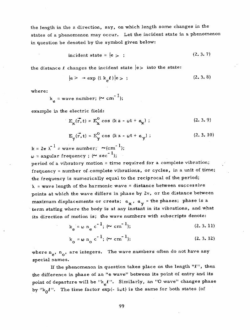
the length in the z direction, say, on which length some changes in the
states of a phenomenon may occur. Let the incident state in a phenomenon
in question be denoted by the symbol given below:
incident state = le > ; (2. 3. 7)
the distance I changes the incident state le> into the state:
le > - exp (i kel )le> ; (2. 3. 8)
where:
k = wave number; (~ cm- );e
example in the electric field:
Ex(r t) = Ex cos (k z - wt + ax ) ; (2. 3.9)
E (r, t) = Eo cos (k z - tt + a ) ; (2. 3. 10)y y y
k = 2w - 1 = wave number; -(cm- );-l
w = angular frequency ; (- sec 1;
period of a vibratory motion = time required for a complete vibration;
frequency = number of.complete vibrations, or cycles, in a unit of time;
the frequency is numerically equal to the reciprocal of the period;
X = wave length of the harmonic wave = distance between successive
points at which the wave differs in phase by 21T, or the distance between
maximum displacements or crests; a x , ay = the phases; phase is a
term stating where the body is at any instant in its vibrations, and what
its direction of motion is; the wave numbers with subscripts denote:
k = n c ; ( cm-); (2. 3. 11)e e
- -
k n c ; ( cm ); (2. 3. 12)
where n e , n o , are integers. The wave numbers often do not have any
special names.
If the phenomenon in question takes place on the length "'I", then
the difference in phase of an "e wave" between its point of entry and its
point of departure will be "k ". Similarly, an "O wave" changes phase
by "k01". The time factor exp(- iwt) is the same for both states (of
99

polarization, say) and does not effect their relative phase. In Equation
(2. 3. 8) the incident state le> is changed on the distance I; this implies
that (as mentioned already in Equation (2. 3. 8)):
e > - exp (i kel )le > ; (2. 3. 13)
as it is seen, the function, which introduces (causes) the changes in the
states is assumed to be in the form of the exponential function, exp (i k )e
Similarly, and incident 10> state changes into
10 > - exp (i k 1)10 > ; (2.3. 14)
the state 0 > is associated with the wave number ko , i. e.,:
-1state 10 > ; wave number k 0 = n0 c ; (2.3. 15)
let us define the wave number "matrix" by:
K= ke le> <el+ kOIO><Ol (2. 3. 16)
The Hermitian adjoint, K + , of the matrix K, Equation (2. 3. 16), is the
matrix:
<x K Ix> <y K x>
K = . (2. 3. 17)<xIKly> <ylKly>
It may happen that in some cases (see Baym, p. 33):
K = K ; (2. 3. 18)
K is then said to be Hermitian.
As an application of operator functions, one may cite the following
example and result:
Suppose that IT(0) > is the state of a system at time t = 0; then
at another time t, the state of the system is given by the equation:
IP(t) > exp (- i Et - )IE > < EI(0)> , (2. 3. 19)
E
where the sum is over a complete set of energy eigenstates of the Hamiltonian,
H, of the system.
100

The row vector <f(t) is given in terms of <P(O) I by:
< (t) = <T(0) (exp(i Ht 4-- ))
<T(0)I exp (i Ht - 1) , (2.3. 20)
where the hermiticity of H is used (see Baym, p. 136). Using Equation
(2. 3. 5), Equation (2. 3. 19) is simply:
Is(t)> = exp (- iHtr - 1) q'(0)> ; (2. 3.21)
equations (2. 3. 19) and (2. 3. 21) are only valid if H does not explicitly
depend on time (Baym, p. 135). The expression IT(t)> in this form
clearly solves the Schroedinger equation:
ih a (t)> = H l(t)> . (2. 3. 22)
2. 4. Heisenberg Representation
On may be often interested in knowing how expectation values of
operators, in the state WI(t)> , change in course of time. If A is an
operator, then its expectation value at time t is:
< A> t = < '(t) IA F(t)> (2. 4. 1)
Assume A not to depend on time explicitly. Using Equation (2. 3. 20) and
(2. 3. 21) one gets:
<A>t = <P(0) lex p (i Ht- 1) A exp(+i Ht4Y 1 IK(O)> ; (2.4. 2)
if we define a time-dependent operator A(t) by:
A(t) = exp (i Ht -h- 1) A exp (- i Ht -r- 1) , (2. 4. 3)
then we can also write:
< A> t = <,(0) A(t) I(0) > . (2.4. 4)
In this equation one can regard the time development of <A> t as occurring
because the operator changes in time, while the state remains the same at all
101

times. This way of regarding the time development of the system is called
the "Heisenberg representation" or "Heisenberg picture." The other
way of looking at the time development, as in Equation .( 2. 3.22 ), where
the operators remain constant in time, but the states change according to
Equation ( 2. 3.22 ), is called the "Schroedinger representation" (or
picture). At t = 0, the states and operators are the same in both repre-
sentations. Both representations give the same results for time dependent
expectation values. We can solve for either the time dependence of the
states in the Schroedinger representation, or for the time dependence of
the operators in the Heisenberg representation.
In the present report the writer applies the Schroedinger represen-
tation to the problem proposed and outlined by Madelung, i.e., the
association between the quantum mechanics and macroscopic hydro-
dynamics.
102