APPLICATION OF THE TOPKAPI MODEL WITHIN THE DMIP 2 PROJECT

8989THTH AMS Annual Meeting, Phoenix, January 2009AMS Annual Meeting, Phoenix, January 2009

Gabriele Coccia(1), Cinzia Mazzetti(2), Enrique A. Ortiz(3) and

Ezio Todini(1)

(1)University of Bologna, Bologna, Italy(2)ProGea Srl, Bologna, Italy

(3)HidroGaia, Paterna (Valencia), Spain

APPLICATION OF THE TOPKAPI MODEL WITHIN THE DMIP 2 PROJECT


TOPKAPI MODEL: A DISTRIBUTED AND PHYSICALLY TOPKAPI MODEL: A DISTRIBUTED AND PHYSICALLY

BASED HYDROLOGIC MODELBASED HYDROLOGIC MODEL

PHYSICALLY BASED MODEL

Physically meaningful parameters whose values can be retrieved from thematic maps (DEM and soil type and land use maps)

Easy calibration

Ungauged catchments

Continuous simulations (climate change, water resources, …)

DISTRIBUTED MODEL

1D outputs (flow, water balance, ect.) everywhere on the catchment

2D maps containing information on soil moisture, snow, evapo-transpiration

REDUCED

COMPUTATIONAL TIMES

AND PARSIMONIOUS

PARAMETRIZATION

Real-time flood forecasting systems

Real-time coupling with hydraulic models

MODEL DESCRIPTION: INTRODUCTION


1. The precipitation is assumed to be constant over the single cell.

2. The entire precipitation infiltrates into the soil until it is saturated (Dunne

Mechanism).

3. The slope of the water table is assumed to coincide with the slope of the

ground, unless the latter is very small (smaller than 0.01%); this constitutes

the fundamental assumption of the Kinematic wave approximation in De

Saint Venant equations, and it implies the adoption of a Kinematic wave

propagation model with regard to horizontal flow, or drainage, in the

unsaturated area.

4. The local transmissivity, like local horizontal subsurface flow, depends on the

integral of the water content profile in the vertical direction (vertical lumping).

5. The saturated hydraulic conductivity is constant with depth in the surface soil layer but much larger than that of deeper layers.

MODEL HYPOTHESESMODEL HYPOTHESES



THE MODEL COMPONENTS THE MODEL COMPONENTS



TOPKAPI is based on the hypothesis that sub-surface flow, overland flow and channel flow

can be approximated using a Kinematic wave approach.

cbat

ηη

−=∂

∂

Sub-surface flow

Overland flow

Channel flow

The integration in space of the non-linear Kinematic wave equations representing subsurface

flow, overland flow and channel flow results in three ‘structurally-similar’ non-linear reservoir

equations.

KINEMATIC APPROACH HYPOTHESIS KINEMATIC APPROACH HYPOTHESIS



( ) s

ss

sus

uo

s VX

XCQQpX

t

V αα2

2 −++=∂∂

Non-linear reservoir equation for SOIL component

( )( ) ααϑϑ

βL

LkC

rs

ss

−=

tan

Soil parameters

rϑ

sϑ

ksh

αs

L

= residual soil moisture content

= saturated soil moisture content

= thickness of the surface soil

layer [m]

= horizontal saturated hydraulic

conductivity [ms-1]

= parameter which depends on

the soil characteristics

MODEL DESCRIPTION: SOIL, SURFACE AND CHANNEL COMPONENTS

SUBSURFACE, SURFACE AND CHANNEL FLOWSSUBSURFACE, SURFACE AND CHANNEL FLOWS

( )( )

( ) O

ooo

o

oo

oooo hXW

XW

WCXWr

t

hXW αα∂

∂−=

( )0

21

tan

nCo

β=

Non-linear reservoir equation for SURFACE component

Surface parameters:

no = Manning’s friction coefficient

for the surface roughness

Channel parameters:

nc= Manning’s friction coefficient for the channel roughness [m-1/3s]

Cross Section Geometry Parameters

2

0cx

x

yBA

⋅=

)tan1( γ+= xx BC

Non-linear reservoir equation for CHANNEL component

( ) ( )

( )34

34

31

32

32

0

tan2c

ucc

c V

Xn

sensQr

t

V

γ

γ−+=

∂

∂


EVAPOEVAPO--TRANSPIRATIONTRANSPIRATION

The Evapo-Transpiration is estimated as a function of the air temperature.

An empirical equation, that relates the reference potential evapo-transpiration, ET0m, to

the compensation factor Wta, to the mean recorded temperature of the month T and

the maximum number of hours of sunshine N of the month, was developed. The

reference potential evapo-transpiration is computed on a monthly basis using one of

the available simplified expressions such as for instance the one due to Thornthwaite

and Mather (1955).

c

mm

b

iTiaiET

=)(

10)(16)(0

( ) ( ) ( )1230

iNinia =

( ) 514.112

1 5∑=

=i

iTb 39275 106751077110179249239.0 bbbc −−− ×+×−×+=

i=1,12 months

MODEL DESCRIPTION: EVAPO-TRANSPIRATION COMPONENT

Monthly reference potential evapo-transpiration

Thornthwaite

Monthly reference potential evapo-transpiration

Doorembosmtam TNWET βα +=0

The relation used, which is structurally similar to the radiation method formula

(Doorembos et al., 1984).


Once coefficients α and β have been found, the equation can be used to obtain actual evapo-

transpitation values for any crop culture at any time step ∆t according to the following

equations:

36002430)(0 ⋅⋅

∆+= ∆

tTNWKET ttac βα Potential evapo-transpiration

>=

≤≤=

≤=

sat

satsat

sat

sat

VVETETa

VVVV

VETETa

VVETa

20

210

10

β

ββ

β

Actual evapo-transpiration

Landuse map

Evapo-transpiration parameters:

Kc = crop factor

β1,β2 = percentages of the saturation volume

MODEL DESCRIPTION: EVAPO-TRANSPIRATION COMPONENT

EVAPOEVAPO--TRANSPIRATIONTRANSPIRATION


SNOW ACCUMULATION AND MELTINGSNOW ACCUMULATION AND MELTING

The snow accumulation and melting module of the TOPKAPI model is driven by a radiation

estimate based upon the air temperature measurements.

At each model pixel the mass and energy balances are computed.

1. Net solar radiation estimation;

HETRad += λ

Net solar radiation Latent heat flux

Sensible heat

ETH λ=Sensible heat:

( )[ ] 00695.05.6062 ETTTRad radal ⋅−−⋅⋅= ηη0ETCET er ⋅=λLatent heat flux

)(695.05.606 0TTC er −−=

The estimation of the radiation is performed by re-converting the latent heat, assumed to

be equal to the potential evapo-transpiration, in the radiation and assuming the sensible

heat to be equal to the latent heat:

ηal = efficiency factor for albedo; ηrad = radiation efficiency factor

MODEL DESCRIPTION: SNOW ACCUMULATION AND MELTING COMPONENT


2. Computation of the Solid and Liquid Percentage of Precipitation;

Threshold temperature Ts

( )σ

sTT

e

TF −−

+

=

1

1σ = 0.6

Ts = 0

3. Estimation of the water mass and energy balances based on the hypothesis of

zero snowmelt;

PZZ ttt +=∆+*

Water mass balance

Energy balance


( )[ ] ( )[ ] ( )TFPTTCCTCPTFTCRadEE salfsisittt ⋅⋅−+++⋅−⋅++=∆+ 00

* 1


4. Comparison of the total available energy with that sustained as ice by the

total available mass at 273 °K;

*0

*ttttsi ETZC ∆+∆+ ≥

=

=

=

∗∆+∆+

∗∆+∆+

tttt

tttt

sm

EE

ZZ

R 0

*0

*ttttsi ETZC ∆+∆+ <

5. Computation of the snowmelt produced by the excess energy; and updating the

water mass and energy budgets.

( ) ( ) smlfsittsmttsi RCTCETRZC +−=− ∆+∆+ 0*

0*

( )

+−=

−=

−=

∗∆+∆+

∗∆+∆+

∗∆+

∗∆+

smlfsitttt

smtttt

lf

ttsittsm

RCTCEE

RZZ

C

ZTCER

0

0

Snowmelt parameter:

Ts = temperature threshold for snow melting

The available energy is

not sufficient to melt part

of the accumulated snow

The available energy is

sufficient to melt part of

the accumulated snow



p

satsvr

vkP

α

ν

= Percolation

PERCOLATION TO DEEPER SOIL LAYERSPERCOLATION TO DEEPER SOIL LAYERS

For the deep aquifer flow, the response time caused by the vertical transport of water

through the thick soil above this aquifer is so large that horizontal flow in the aquifer can be

assumed to be almost constant with no significant response on one specific storm event in

a catchment (Todini, 1995). Nevertheless, the TOPKAPI model accounts for water

percolation towards the deeper soil layers even though it does not contribute to the

discharge.

The percolation rate from the upper soil layer is assumed to increase as a function of the soil

water content according to an experimentally determined power law (Clapp and Hornberger,

1978. Empirical Equations for some soil hydraulic properties; Liu et al., 2005).

Percolation parameters:

ksv

αp

= vertical saturated hydraulic conductivity [ms-1]

= parameter which depends on the soil characteristics

Soil type map

(pedology)

MODEL DESCRIPTION: PERCOLATION COMPONENT


MODEL APPLICATION: DMIP 2 SIERRAMODEL APPLICATION: DMIP 2 SIERRA--NEVADA BASINSNEVADA BASINS

TOPKAPI model has been applied within the DMIP 2 to the North

Fork American River Basin and the East Fork Carson River Basin

MODEL APPLICATION: BASINS DESCRIPTION


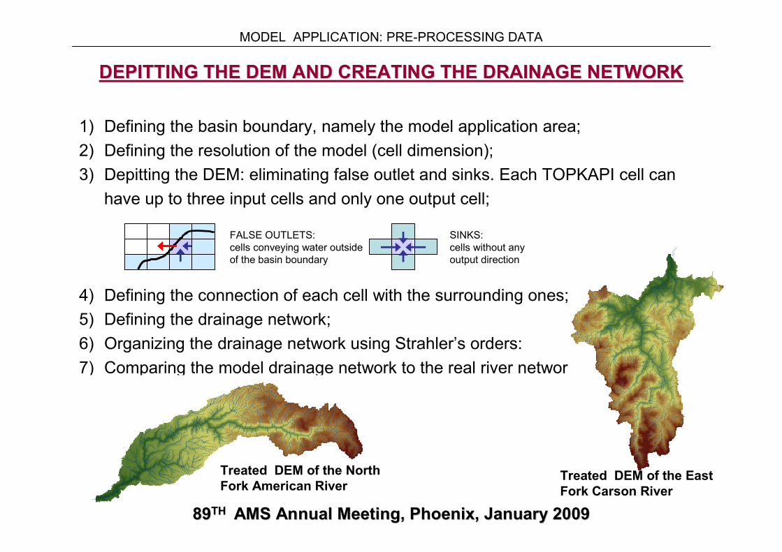
DEPITTING THE DEM AND CREATING THE DRAINAGE NETWORK DEPITTING THE DEM AND CREATING THE DRAINAGE NETWORK

1) Defining the basin boundary, namely the model application area;

2) Defining the resolution of the model (cell dimension);

3) Depitting the DEM: eliminating false outlet and sinks. Each TOPKAPI cell can

have up to three input cells and only one output cell;

4) Defining the connection of each cell with the surrounding ones;

5) Defining the drainage network;

6) Organizing the drainage network using Strahler’s orders:

7) Comparing the model drainage network to the real river network.

FALSE OUTLETS:

cells conveying water outside

of the basin boundary

SINKS:

cells without any

output direction

Elevation [m]

High : 3468.3

Low : 1462.26

MODEL APPLICATION: PRE-PROCESSING DATA

Treated DEM of the North

Fork American RiverTreated DEM of the East

Fork Carson River


SETTING THEMATIC MAPS SETTING THEMATIC MAPS -- SELECTING INITIAL PARAMETER VALUESSELECTING INITIAL PARAMETER VALUES

SOIL TYPE

and

LAND USE

MODEL APPLICATION: PRE-PROCESSING DATA

rϑ = residual soil moisture content

sϑ = saturated soil moisture content

L = thickness of the surface soil layer

ksh = horizontal saturated hydraulic conductivityαs = parameter for subsurface flow

ksv = vertical saturated hydraulic conductivityαp = parameter for percolation

no = Manning’s friction coefficient for the surface roughness

Kc= crop factor

nc

B

= Manning’s friction coefficient for the channel roughness

= Width of the rectangular channel

γ = slope of channel sides (for triangular sections)

β1, β2= evapo-transpiration parameters

= temperature threshold for snow accumulation-meltingTs


MODEL APPLICATION: HYDRO-METEROLOGICAL DATA

!(

!(

!(

!(

#*

#*

Blue Lake

Poison Flat

Ebbett Pass

Spratt Creek

GardnerVille

Markleeville

#

Huysink

Blue Canyon

North Fork Dam

1/10/1987 31/12/20021/10/1988 1/10/1997

WARM UP CALIBRATION VALIDATION

1/10/1990 31/12/20021/10/1989 1/10/1997

WARM UP CALIBRATION VALIDATION

HYDROHYDRO--METEOROLOGICAL DATAMETEOROLOGICAL DATA

Gridded hourly precipitation data

Gridded hourly temperature data

Observed hourly streamflow

data at North Fork Dam for

the American River, and at

Gardnerville and Markleeville

for the Carson River

Observed daily Snow Water

Equivalent data at Blue

Canyon and Huysink for the

American River, and at

Poison Flat, Ebbett Pass,

Blue Lake and Spratt Creek

for the Carson River.


MODEL APPLICATION: CALIBRATION RESULTS, AMERICAN RIVER, LONG-TERM PERIODS


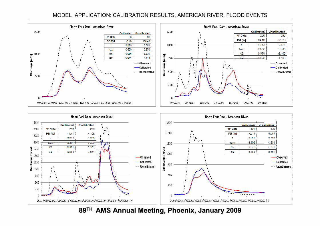
MODEL APPLICATION: CALIBRATION RESULTS, AMERICAN RIVER, FLOOD EVENTS


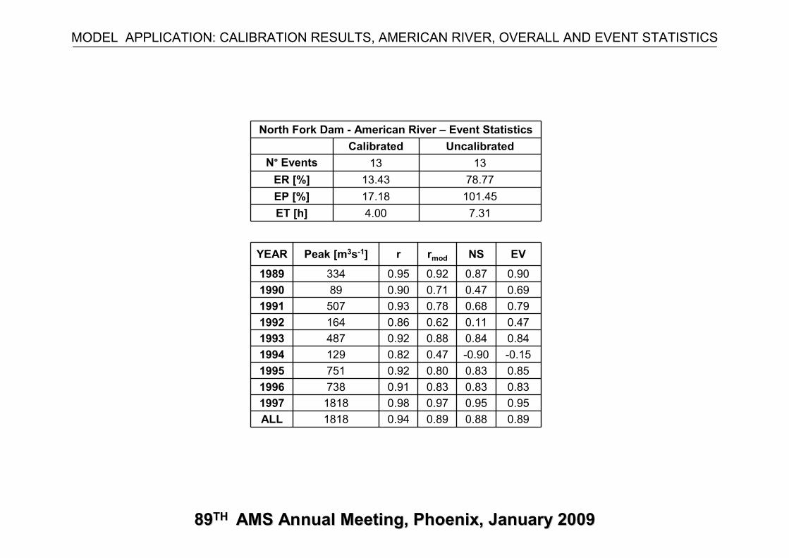
MODEL APPLICATION: CALIBRATION RESULTS, AMERICAN RIVER, OVERALL AND EVENT STATISTICS

North Fork Dam - American River – Event Statistics

Calibrated Uncalibrated

N° Events 13 13

ER [%] 13.43 78.77

EP [%] 17.18 101.45

ET [h] 4.00 7.31

YEAR Peak [m3s-1] r rmod NS EV

1989 334 0.95 0.92 0.87 0.90

1990 89 0.90 0.71 0.47 0.69

1991 507 0.93 0.78 0.68 0.79

1992 164 0.86 0.62 0.11 0.47

1993 487 0.92 0.88 0.84 0.84

1994 129 0.82 0.47 -0.90 -0.15

1995 751 0.92 0.80 0.83 0.85

1996 738 0.91 0.83 0.83 0.83

1997 1818 0.98 0.97 0.95 0.95

ALL 1818 0.94 0.89 0.88 0.89


MODEL APPLICATION: CALIBRATION RESULTS, CARSON RIVER, LONG-TERM PERIODS


MODEL APPLICATION: CALIBRATION RESULTS, CARSON RIVER, OVERALL AND EVENT STATISTICS

Gardnerville – Carson River

YEAR Peak [m3s-1] PB [%] r rmod NS EV

1991 38 88.2 0.85 0.47 -0.72 -0.23

1992 27 137.8 0.94 0.44 -2.12 -0.55

1993 84 -1.7 0.92 0.83 0.81 0.81

1994 31 79.3 0.92 0.50 -0.46 0.02

1995 167 -19.2 0.95 0.81 0.86 0.89

1996 221 3.5 0.93 0.86 0.86 0.86

1997 527 0.8 0.90 0.72 0.80 0.80

ALL 527 13.9 0.89 0.81 0.79 0.80

Gardnerville - Carson River – Event Statistics

Calibrated UncalibratedN° Events 4 4

ER [%] 6.26 329.48

EP [%] 38.34 699.20

ET [h] 1.50 2.75

Markleeville – Carson River

YEAR Peak [m3s-1] PB [%] r rmod NS EV

1991 39 102.3 0.84 0.44 -1.28 -0.46

1992 27 160.5 0.93 0.40 -3.51 -1.02

1993 74 3.5 0.92 0.79 0.79 0.79

1994 32 110.0 0.94 0.47 -1.20 -0.23

1995 168 -7.7 0.96 0.92 0.91 0.92

1996 200 19.2 0.93 0.91 0.84 0.86

1997 385 13.5 0.94 0.83 0.88 0.88

ALL 385 28.0 0.91 0.91 0.79 0.82

Markleeville - Carson River – Event Statistics

Calibrated UncalibratedN° Events 5 5

ER [%] 24.75 211.43

EP [%] 30.28 382.71

ET [h] 7.20 7.80


MODEL APPLICATION: CALIBRATION RESULTS, CARSON RIVER, SNOW WATER EQUIVALENT

Blue Lakes – 2456 m Ebbets Pass– 2672 m

Poison Flats – 2358 m Spratt Creek – 1864 m


CONCLUSION

1) The TOPKAPI model well reproduces the streamflow series in basins with a

complex hydrological regime, it can reproduce both flood and low water events

with good accuracy;

2) The TOPKAPI model was born for low elevation catchments, where the snow

melting component is not much significant and its snow accumulation and

melting module is simple; however, its application in high elevation basins is

feasible and the results are not extremely precise, but good on the whole;

3) The experience in calibrating the model and the comparison between

calibrated and uncalibrated simulations show that literature parameter values

are usually too small for the superficial soil layer conductivity; using the

TOPKAPI model in ungauged basins, it is necessary to account for that;

4) As shown, in the application in the Carson River, by the results at Markleeville

using the calibration performed at Gardnerville, the TOPKAPI model is capable

to produce optimal simulations in ungauged points of the basin.

CONCLUSIONCONCLUSION


THANK YOU FOR YOUR ATTENTION!


EVALUATION INDEXES

( )100

1

1 ×−

=

∑

∑

=

=N

i

i

N

i

ii

O

OS

PB

−

−

−=

∑ ∑∑ ∑

∑∑∑

= == =

===

N

i

N

i

ii

N

i

N

i

ii

N

i

i

N

i

i

N

i

ii

OONSSN

OSOSN

r

1

2

1

2

1

2

1

2

111

{ }{ }obssim

obssimrrσσσσ,max

,minmod = Modified Correlation Coefficient

Percent Bias

Correlation Coefficient

( )

( )∑

∑

=

=

−

−−=

N

i

i

N

i

ii

OO

OS

NS

1

2

1

2

1 Nash-Sutcliffe Efficiency

( ) ( )

( )∑

∑ ∑

=

= =

−

−−−

−=N

i

i

N

i

N

i

iiii

OO

OSN

OS

EV

1

2

2

1 1

1

1 Explained Variance


EVALUATION INDEXES

1001 ×=∑=

avg

N

i

i

NY

B

ER

Absolute Peak Time Error

Percent Absolute Event Runoff Error [%]

100,

1

,,

×−

=∑=

avgp

N

i

ipsip

NQ

QQ

EP Percent Absolute Peak Error [%]

N

TT

ET

N

i

ipsip∑=

−= 1

,,

( )

N

OS

RMSE

N

i

ii∑=

−= 1

2

Root Mean Square Error


( )( )∫=L

dzzkT

0

~ϑ

rs

rzz

ϑϑϑϑ

ϑ−−

=)(

)(~

∫∫∫ ≠

=Θ⇒=Θ

LLL

dzzL

dzzL

dzzL

000

)(~1

)(~1~

)(~1~ α

α

α ϑϑϑ

( ) ⇒⋅= αϑϑ )(~

)(~

zkzk s( )∫=

L

s dzzkT0

~ αϑ= Transmissivity, if

se

where:

4th MODEL HYPOTESIS


( )

( )

Θ=

=+Θ

−

αβ∂∂

∂∂

ϑϑ~

tan

~

Lkq

px

q

tL

s

rsContinuity equation

Dynamic equation

( ) s

ss

sus

uo

s VX

XCQQpX

t

V αα2

2 −++=∂∂

Non-linear reservoir equation for SOIL component

( )( ) ααϑϑ

βL

LkC

rs

ss

−=

tan

Soil type map

(pedology)

Groundsurface

p

Qs

Qs

Qo

Soil parameters

rϑ

sϑ

ksh

αs

L

= residual soil moisture content

= saturated soil moisture content

= thickness of the surface soil layer [m]

= horizontal saturated hydraulic conductivity [ms-1]

= parameter which depends on the soil characteristics

MODEL DESCRIPTION: SOIL COMPONENT

SUBSURFACE FLOWSUBSURFACE FLOW


==

−=

o

ooo

o

o

oo

o

hChn

q

x

qr

t

h

αβ

∂∂

∂∂

3

52

1

)(tan1

Continuity equation

Dynamic equationOverland water surface

ro

Land use map

OVERLAND FLOW OVERLAND FLOW

( )( )

( ) O

ooo

o

oo

oooo hXW

XW

WCXWr

t

hXW αα∂

∂−=

( )0

21

tan

nCo

β=

Non-linear reservoir equation for SURFACE component

Surface parameters:

no = Manning’s friction coefficient for

the surface roughness [m-1/3s]

The input to the surface water model is the precipitation excess (r0) resulting from the

saturation of the surface soil layer.

MODEL DESCRIPTION: SURFACE COMPONENT


Strahler’s orders

CHANNEL FLOW: KINEMATIC WAVECHANNEL FLOW: KINEMATIC WAVE

TRIANGULAR cross-section Continuity equation

Dynamic equation

MODEL DESCRIPTION: CHANNEL COMPONENT

( )

=

−+=

38

35

32

32

0

tan

sin

2c

c

c

cucc

c

y

n

sq

qQrt

V

γ

γ

∂∂

2

0cx

x

yBA

⋅=

)tan1( γ+= xx BC

Non-linear reservoir equation for CHANNEL component

( ) ( )

( )34

34

31

32

32

0

tan2c

ucc

c V

Xn

sensQr

t

V

γ

γ−+=

∂

∂

Rectangular cross-section

parameters:nc

B

= Manning’s friction coefficient for

the channel roughness [m-1/3s]

= Width of the rectangular channel [m]

γ = Slope of the channel sides


CHANNEL FLOW: MUSKINGUMCHANNEL FLOW: MUSKINGUM--CUNGECUNGE--TODINITODINI

Todini E., 2007. A mass conservative and water storage consistent variable parameter

Muskingum-Cunge approach. Hydrol. Earth Syst. Sci., 11:1645–1659.

MODEL DESCRIPTION: CHANNEL COMPONENT

It is possible to use the Muskingum-Cunge-Todini routing method, as an

alternative to the Kinematic non-linear reservoir, for channels with slope smaller

than 0.1%.

10300201111 qcqcqcq ⋅+⋅+⋅=

**

**

11

1

tttt

tt

DC

DCC

∆+∆+ ++

++−=

**

**

21

1

tttt

tt

DC

DCC

∆+∆+ ++

−+=

*

*

**

**

31

1

t

tt

tttt

tt

C

C

DC

DCC ∆+

∆+∆+ ++

+−=

tttttt OCICICO 321ˆ ++= ∆+∆+

x

tcC

t

tt ∆

∆=β

*

xcBS

QD

tt

tt ∆=

0

*

β

t

tt

Q

Ac=β

Documents

APPLICATION OF THE TOPKAPI MODEL WITHIN THE DMIP 2 PROJECT