A APPLICATION OF THE SDC OPTIMAL CONTROL

INCLUDING FOURTH BODY EFFECTS LGORITHM TO LOW-THRUST ESCAPE AND CAPTURE

Gregory J. Whiffen and Jon A. Sims Navigation and Mission Design Section, Jet Propulsion Laboratory,

California Institute of Technology, Pasadena, CA 91 109 Gregory.J.Whiffen@jpl.nasa.gov, Jon.A.Sims@jpl.nasa.gov

An application of the new optimization algorithm called Static/Dynamic Control (SDC) to design low-thrust escape and capture trajectories is pre- sented. SDC is a general optimization method that is distinct from both parameter optimization and the calculus of variations. Trajectories are in- tegrated with a multi-body force model and feature ~ ~~~~ solar electric propulsion with a speEifiCimpdG that is a function of the engine throttle. Test prob- lems include interplanetary scale trajectories that capture or escape at the Earth and Mars. Optimizing capture and escape trajectories with a multi- body force model results in a significant improvement in the mass delivered compared to existing two-body formulations. A variety of optimal escape and capture trajectories types are identified and classified. Three-body (e.g. Sun and Earth gravitating) optimal escape and capture is compared to four-body (e.g. Sun, Earth, and Moon gravitating) optimal escape and capture. SDC is robust for this appiication and does not require a good initial guess.

1. INTRODUCTION

Low-thrust electric propulsion is increasingly being selected as the propulsion system of choice for future high AV interplanetary missions.[lI The higher efficiency of electric propulsion compared to traditional chemical propulsion results in larger payload delivered or shorter flight times. The successful Deep Space 1 mission demonstrated the reliability of electric propulsion.

Optimizing low-thrust trajectories and, in particular, trajectories that include escape and capture is inherently difficult. Low thrust engines typically operate for days, months or even years. The continuous operation associated with low thrust significantly increases the optimization complexity. Long continuous thrusting renders approximations and tools used for chemical propulsion trajectories inaccurate or useless. High fidelity modeling of escape and capture requires a multi-body force model. However, a multi-body force model will only further compound the optimization complexity. To fully optimize an escape or capture trajectory, the origin or destination of the trajectory must be taken into account. Typically this involves an interplanetary scale trajectory leg. However, optimizing a trajectory involving both an interplanetary leg and a planet centered spiral introduces two very different time and distance scales into mathematical formulation. Widely varying time and distance scales are known to create difficulty for optimization.

Many researchers have sought to avoid the aforementioned difficulties by using one or more simplifying assumptions. A common method is to use a two-body approximation and/or a divide and conquer approach for escape and c a p t ~ r e . [ ~ > ~ ] For example, an Earth to Mars capture trajectory can be roughly approximated as two separate problems. First, an optimal interplanetary trajectory from Earth to Mars is obtained such that the incoming V, at Mars is near zero. Second, a Mars centered spiral problem is solved. The spiral problem begins with two-body energy of zero and ends with the target capture orbit around Mars. Although

1

two-body formulations are much simpler to solve, they do not take full advantage of the strong multi-body effects that occur near zero energy, and they can not optimize the trajectory end-to-end. The results in this paper demonstrate that the optimization of trajectories of this type should not be separated into two or more independent problems. There is a significant performance penalty for separating the problem near zero energy.

The high fidelity optimization of low-thrust escape and capture with a multi-body force model is the main objective of this research. It is also an objective of this research to optimize trajectories that involve both an interplanetary leg and planet centered spirals without dividing the trajectory up into subproblems (based on length and time scales) and optimizing each independently. The research presented in this paper is an extension of earlier research[*] into trajectories that are inherently three-body problems (planet, Sun, and spacecraft.) This research focus on trajectories that are inherently four-body problems (planet, Sun, Moon, and spacecraft).

An important feature of the SDC approach is its ability to exploit multi-body phenomena. It is not necessary to specify intermediate flyby bodies or multi-body interactions on input. SDC can incorporate Tfficient interactions on its own. This is in contrast to many existing optimization methods. SDC does not require a good initial trajectory guess to begin the optimization. SDC’s ability to begin with poor guesses and locate favorable interactions results in the identification of non-obvious, yet highly efficient four-body escape and capture trajectories.

2. APPROACH

Existing methods for optimizing low-thrust trajectories are classified as either direct or indirect. Direct approaches parameterize the trajectory a d sdve the parameterized problem using a gradiefit based nonlinear programming method, or a hueristic method such as simulated annealing. Direct methods typically remove the explicit time dependence in the optimal formulation by parameterizing the trajectory. Indirect approaches are based on the calculus of variations, resulting in a two point boundary value problem.i5I Indirect methods do not remove the explicit time dependence of the trajectory problem, rather it is soived as an optimal control problem. Calculus of variations methods are often limited to a single body (Sun or planet) force model due to the sensitivity of the method.

The optimization method used in this research is called Static/Dynamic Control or SDC.16] SDC is a new, general optimization algorithm which was derived to address a general class of problems with the same structure as low-thrust optimization. SDC best fits into the direct method category. However, unlike other direct methods, the explicit time dependence of the optimization problem is not removed by parameterization. The SDC optimization algorithm is a form of optimal control. Unlike many other optimization approaches, SDC can be used with the highest fidelity space flight simulators available. SDC is a robust optimization method that can handle the large changes in length and time scales that occur in problems with both interplanetary legs and planet centered spirals.

The trajectories analyzed include escape from a high Earth orbit to a rendezvous with Mars and escape from a high Mars orbit to capture into Earth orbit. Two-body capture and three-body capture (Moon not gravitating) are compared to four-body capture (Moon gravitating) performance.

2.1 The General SDC Problem Structure

SDC is a general optimization method designed to solve a class of mathematical problems. The SDC optimization algorithm is based in part on the Hamilton, Bellman, Jacobi dynamic programming equation.[7] Unlike traditional differential dynamic programming methods, SDC is constructed to solve highly nonlinear and non-convex problems with a dual dynamic and parametric structure. Optimal solutions generated by SDC satisfy both necessary and sufficient conditions of optimality.

2

Three distinct variable classes are recognized by SDC. The first is the dynamic control vector which is a function of time. The dynamic control is analogous to control in optimal control theory. The vector v( t ) is used to represent the dynamic control at time t . The second variable class is the static control vector which can be thought of as the control in parameter optimization. The vector w is used to represent the static control. Both the static and dynamic control encompass design variables that are under direct control by the engineer. In addition to the static and dynamic controls, SDC recognizes a time dependent state vector. The state vector encompasses variables not under the direct control of the engineer. The vector z ( t ) is used to represent the state a t time t .

The general objective or cost function of SDC can be written as the addition of a time-integrated cost and a sum of point-in-time costs:

N

J = lotN F(z( t ) , v( t ) , w, t)dt + G(z(t i ) , v(t i) , w , t i , i). i=l

The goal of SDC is to optimize J by choosing the optimal or “best” ~- dynamic control v ( t ) at all time instants t E (t0,tN) simultaneously with thebptimal static control w. The objective J can be either minimized or maximized in value. The general functions F and G in Eq. (1) are selected to best represent the design and control objectives for a specific application. The times t, are assumed to lie between t o and tN for i = 1 ,2 , ..., N - 1. The functions F and G are required to be twice continuously differentiable with respect to IC, v, and w. The functions F and G do not need to be continuous in time t .

In addition to the objective Eq. (l), SDC requires an ordinary differential equation which describes the time evolution of the state vector z, and a function that specifies the initial state z( t = t o ) :

The &te fiunction T is required to be twice continuous!y differentiable with respect t~ z, z’, and w. R=svever, LIIV SLCLLV i u i u i u n 1 uues not need to be coniinuous in time t . The initiai condition can be given and fixed, or it can be a function of the static control w. The function I7 is required to be once continuously differentiable with respect to w.

1-1- f... -~~ m -I ~ ~

SDC optionally allows two types of constraints on the formulation Eqs. (1) and ( 2 ) . The first type is ordinary constraints of the general form:

L(z ( t ) , w(t), w , t ) 2 0 andlor K ( z ( t ) , v ( t ) , w, t ) = 0, (3)

The linear or nonlinear vector functions L and K are selected to represent constraints on the engineering problem. An example of a constraint of this type is a minimum allowed distance between the Sun and a spacecraft to avoid spacecraft overheating.

The second type of constraint SDC allows are “control dynamic” constraints. Control dynamic con- straints represent any physical or practical engineering constraints on the time evolution of the dynamic control vector w(t). The control dynamic constraints have the general form:

I f ( W , W , t , l ) for t = t o to tl I

I f(UN,W,t,N) f o r t = t N - 1 to tN. I The vector functions f(ui, w, t , i) are selected to properly represent the limitations on the time evolution of v( t ) . The number of periods N may be chosen arbitrarily. The functions f are parameterized by a parameter vector ui, the static parameter vector W , and time t . The functions f can be used to effectively limit or

3

constrain the SDC algorithm to consider only solutions v ( t ) which are of the form of Eq. (4). The time intervals ti to ti+l are called “periods.” The dynamic parameter vector ui is constant within each period i, i = 1 , 2 , ..., N . For example, the simplest useful set of functions f is f (ui, w, t , i) = ui. The dynamic control vector v ( t ) may be optimized such that v ( t ) is constant over each period, allowing changes only at period interfaces ti. Alternatively, v ( t ) may be subject to a dynamic limitation that allows v ( t ) t o vary within each period, either continuously or discontinuously.

If SDC is used with control dynamic constraints, then the algorithm is called the period formulation of SDC. If no control dynamic constraint is used then the algorithm is called the fully continuous formulation of SDC. In this research, the period formulation of SDC was used to constrain the trajectory optimization to only allow changes in the thrust direction and magnitude at regular time intervals. The regular time intervals represent the practical limitations of spacecraft control resulting from communications and/or duty cycles.

2.2 Application of SDC to Trajectory Optimization

In this application, the state vector x ( t ) is defined to be the spacecraft state at any given time t. The components of the state vector x ( t ) are defined as follows,

x ( t ) =

x coordinate of spacecraft y coordinate of spacecraft z coordinate of spacecraft x velocity of spacecraft y velocity of spacecraft z velccitjl c f spacecraft mass of the spacecraft.

The Jxrqamic -J - centre! v(t\ J is dcfined to be the electric propulsion thrirst vector,

1 x component of thrust y component of thrust z component of thrust .

The components of the static control vector w are defined to be

1 Date of Earth launch total f l i g h t t ime.

w = [ ;; ] = [ (7)

The SDC algorithm is not limited to the definition Eqs. (5), (6), and (7). Additional control and state dimensions can be added. For example, the static control w could be augmented with design parameters like solar array size, launch V, components, or forced intermediate flyby dates. The state vector x could be augmented with a state representing the total spacecraft radiation dose.

The equation used to describe the time evolution of the state is

dx - = T ( x , v, w, t ) = z7 t dt A

3 x 7 ( t )

L

x velocity of spacecraft y velocity of spacecraft z velocity of spacecraft

x acceleration of spacecraft y acceleration of spacecraft z acceleration of spacecraft

mass flow rate

4

The mass flow rate m is provided by a polynomial fit to the performance of the NSTAR 30-cm ion thrusterls], a version of which was used on Deep Space 1. The specific impulse is not constant, but depends on the engine throttle level.

The function r ( w ) used in this research provides the position and velocity of the spacecraft in some specified initial captured orbit at either Mars or Earth.

Constraints of the form of Eq. (3) are used to constrain the thrust and reach intermediate and final target bodies. The maximum thrust is constrained by the performance of the thruster(s) and the power available from the solar array at a given heliocentric radius. The target final state used in this research is either an orbital energy, a circular orbit, or a massless rendezvous constraint. The form of the fixed final energy constraint used in this analysis is

The energy Etarget is the final orbital energy with respect-to the target body. The relative velocity between the spacecraft and the target body is urez = Uspacecra f t - U b o d y where uspacecraft = { Q ( ~ N ) , q , ( t ~ ) , 2 6 ( t N ) } .

The parameter jLbody iS the gravitational constant of the target. The variable TTel = T s p a c e c r a f t - ?‘body is the separation between the spacecraft and target body. When constraint Eq. (9) is enforced, the optimization will generate an optimal trajectory that achieves a specified orbital energy Etarget. A circular orbit is achieved by using three separate constraints of the form of Eq. (3).

I Irrd 1 1 = I l r spacecra f t - T b o d y I I = R t a r g e t l l u r e l l l = urel . T r e l = 0. (10) rTP,l

The first constraint requires the given circular orbit radius Rtarget. The second constraint requires the relative velocity magnitude between the spacecraft and body to be consistent with a circular orbit. The third constraint requires the relative velocity to be perpendicular to the separation vector. The form of the massless rendezvous constraint (two-body approximation of capture) is

2 1 : 3 ( t N ) = rbody 24:6 ( t N ) = w b o d y (11)

where the vector position of the target body T b o d y and the vector velocity u b o d y are given by the JPL DE405 ephemeris. This constraint is used to compare the performance of optimal two-body capture to optimal multi-body capture. The objective used for comparisons was to maximize the final spacecraft mass q ( t ~ ) .

3. RESULTS

3.1 Mars Escape Spiral to Earth Capture Spiral

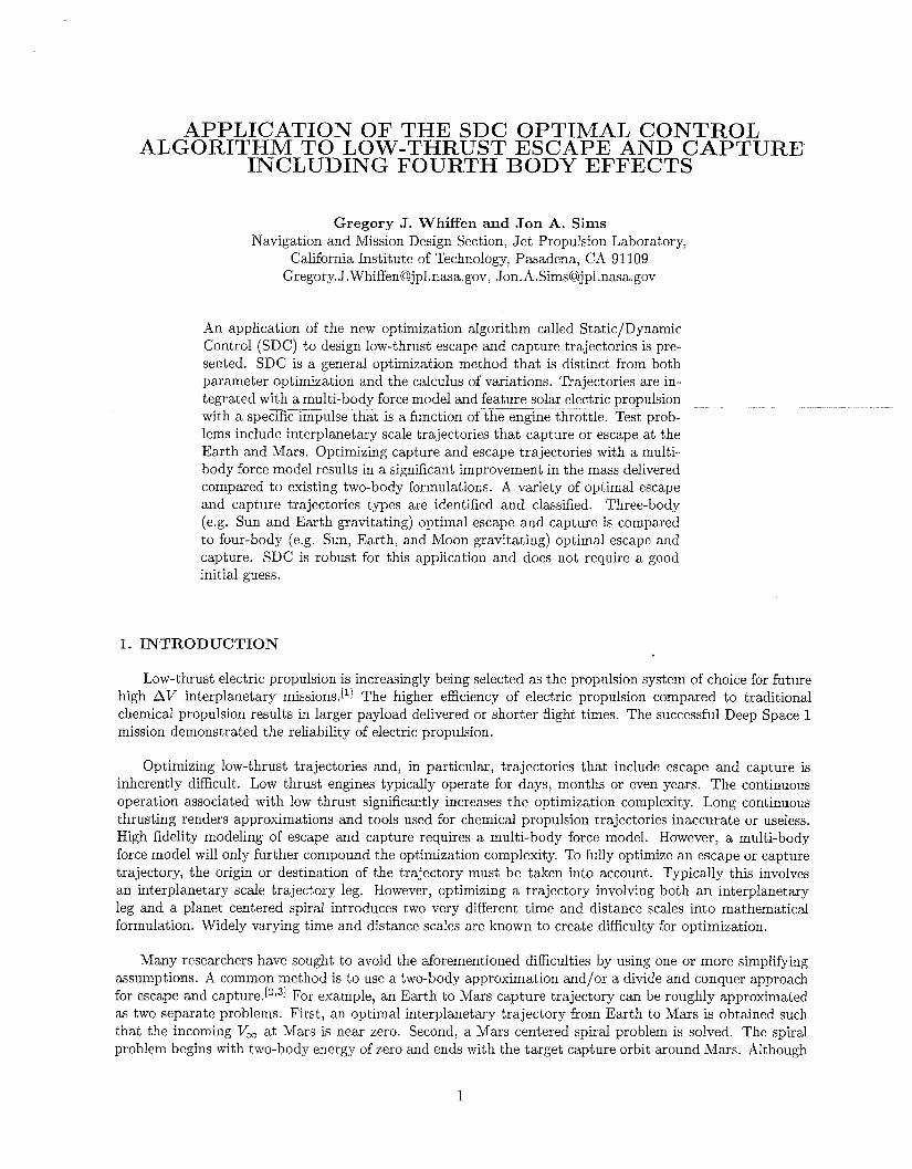
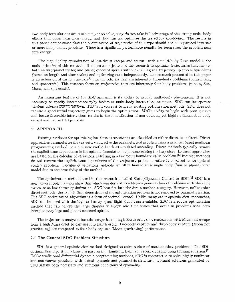
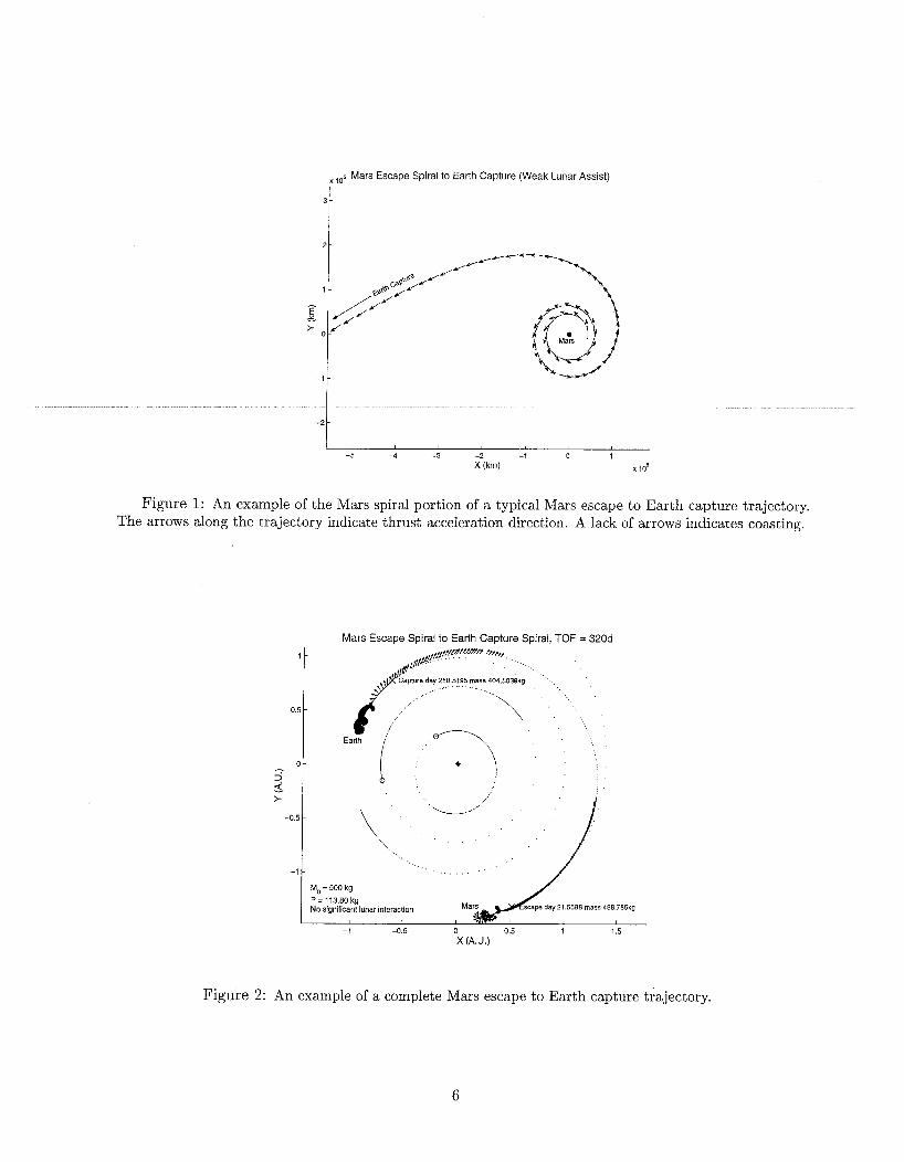
The Mars escape to Earth capture trajectory begins in orbit around Mars on April 15, 2005. The initial Mars orbit has eccentricity of .05, a semi-major axis of 45,000 km, and an inclination of 5 O relative to the ecliptic. The spiral at Mars changes little between test cases. Some Mars spirals include a short coast, some do not, but all have the same number of revolutions to escape. Figure 1 is a plot of a typical Mars escape spiral. The Mars escape is used as a plausible trajectory origin (Mars sample return), but was not the focus of this investigation. The focus is on the capture into the Earth-Moon system. The target orbit at Earth was either a captured orbit with a fixed periapsis of 100,000 km or an orbit with a fixed, negative final energy of -1.4 q. Figure 2 is a plot of a typical complete trajectory. The initial spacecraft mass in Mars orbit is 500 kg. The solar array power is 11 kw at 1 A.U. Two NSTAR 30-cm ion thrusters are available on the spacecraft. The flight time is varied between 295 and 390 days.

Capture in the Earth-Moon system can be classified as a “four-body” problem because the list of signif- icant gravitating bodies must include the Moon in addition to the Sun and Earth. Obviously, the four body problem generates a complex optimization space. SDC is uniquely suited to explore the optimal trajectories

5

x1Q6 Mars Escape Spiral to Earth Capture (Weak Lunar Assist) I

-7 1 8

-5 -4 -3 -2 -1 Q 1 X (km) io'

Figure 1: An example of the Mars spiral portion of a typical Mars escape to Earth capture trajectory. The arrows along the trajectory indicate thrust acceleration direction. A lack of arrows indicates coasting.

Mars Escape Spiral to Earth Capture Spiral, TOF = 320d

a

- 2 Y

t

-0

M, = 500 kg / P=113.80kg No significant lunar interaction

-1 -0.5 0 0.5 1 1.5 X (A.U.)

Figure 2: An example of a complete Mars escape to Earth capture trajectory.

6

that exist in the four-body case. SDC does not require a good guess to begin the optimization. It is this feature that is used to explore the complex optima space of four-body capture and escape. A large number of poor initial guesses and different initial conditions were generated to begin separate optimizations. The purpose of this procedure is to investigate (with as little bias as possible) the range of available, locally optimal trajectories. Hundreds of different optima.1 escape and capture trajectories were obtained in this way. A classification system was developed and all trajectories were classified as belonging to one of several distinct minima types. Escape and capture exhibits a symmetry in that, capture minima have analogous escape minima.

The relative performance of four-body optima can be compared to three-body optima. Three-body (Moon not gravitating) results used for comparison were obtained from reference [4]. Both three- and four- body solutions can be compared to two-body solutions. Two-body solutions are obtained by setting both the Earth and Moon mass to zero and using constraint Eq. (11) for a two-body capture a t Earth.

Reference [4] found that there are at least two classes of optimal captures for flight time limited (< 385 days) three-body capture. One minima type has a high final Earth orbit eccentricity ~ and the other minima type has a low finalT?bit eccentricity. -The-rdativesuperio%y of the minima types depends on the&llowed flight time. Minima of low-eccentricity type are characterized by continuous engine operation throughout the capture and spiral. Minima of the high eccentricity type are characterized by thrust arcs that are roughly centered on the periapsis.

__

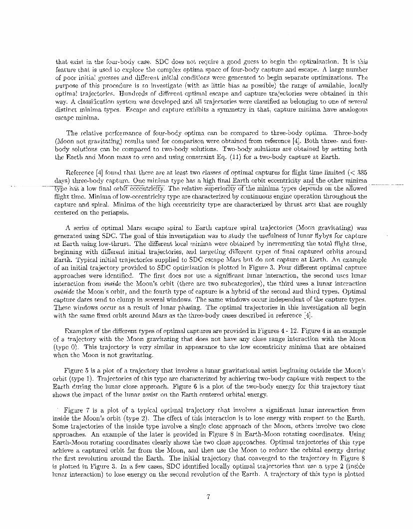
A series of optimal Mars escape spiral to Earth capture spiral trajectories (Moon gravitating) was generated using SDC. The goal of this investigation was to study the usefulness of lunar flybys for capture at Earth using low-thrust. The different local minima were obtained by incrementing the total flight time, beginning with different initial trajectories, and targeting diRerent types of final captured orbits around Earth. Typical initial trajectories supplied to SDC escape Mars but do not capture at Earth. An example of an initial trajectory provided to SDC optimization is plotted in Figure 3. Four different optimal capture approaches were identified. The first does not use a significant lunar interaction, the second uses lunar interaction from inside the Moon’s orbit (there are two subcategories), the third uses a lunar interaction outside the Moon’s orbit, and the fourth type of capture is a hybrid of the second and third types. Optimal capture dates tend to clump in several windows. The same windows occur independent of the capture types. These windows occur as a result of lunar phasing. The optimal trajectories in this investigation all begin with the same fixed orbit around Mars as the three-body cases described in reference [4].

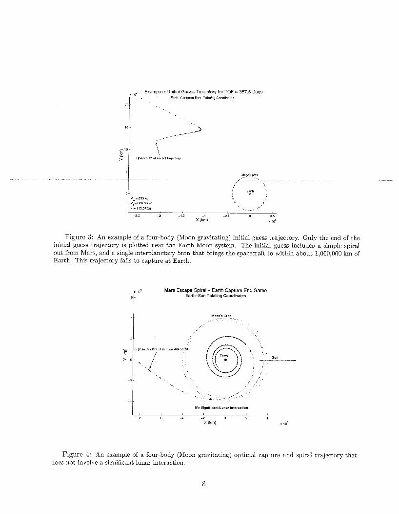
Examples of the different types of optimal captures are provided in Figures 4 - 12. Figure 4 is an example of a trajectory with the Moon gravitating that does not have any close range interaction with the Moon (type 0) . This trajectory is very similar in appearance to the low eccentricity minima that are obtained when the Moon is not gravitating.

Figure 5 is a plot of a trajectory that involves a lunar gravitational assist beginning outside the Moon’s orbit (type 1). Trajectories of this type are characterized by achieving two-body capture with respect to the Earth during the lunar close approach. Figure 6 is a plot of the two-body energy for this trajectory that shows the impact of the lunar assist on the Earth centered orbital energy.

Figure 7 is a plot of a typical optimal trajectory that involves a significant lunar interaction from inside the Moon’s orbit (type 2). The effect of this interaction is to lose energy with respect to the Earth. Some trajectories of the inside type involve a single close approach of the Moon, others involve two close approaches. An example of the later is provided in Figure 8 in Earth-Moon rotating coordinates. Using Earth-Moon rotating coordinates clearly shows the two close approaches. Optimal trajectories of this type achieve a captured orbit far from the Moon, and then use the Moon to reduce the orbital energy during the first revolution around the Earth. The initial trajectory that converged to the trajectory in Figure 8 is plotted in Figure 3 . In a few cases, SDC identified locally optimal trajectories that use a type 2 (inside lunar interaction) to lose energy on the second revolution of the Earth. A trajectory of this type is plotted

7

105 Example of Initial Guess Trajectory for TOF = 357.5 Days

Earth-Centered Non-Rotating Coordinates 2ol . . . . - - . 15

- IF- t.

-

\ Spaceman at end of trajectory

~.,, ,,-

Mo = 500 kg. M, = 386.63 kg

P = 113.37 kg

-2.5 -2 -1.5 -1 -0.5 0 0.5

x (h) x loe

Figure 3: An example of a four-body (Moon gravitating) initial guess trajectory. Only the end of the initial guess trajectory is plotted near the Earth-Moon system. The initial guess includes a simple spiral out from Mars, and a single interplanetary burn that brings the spacecraft to within about 1,000,000 km of Earth. This trajectory fails to capture at Earth.

Mars Escape Spiral - Earth Capture End Game Earth-Sun Rotating Coordinates

No Significant Lunar Interaction

-8 -6 -4 -2 0 2 4

X (km) lo5

Figure 4: An example of a four-body (Moon gravitating) optimal capture and spiral trajectory that does not involve a significant lunar interaction.

8

Mars Escape spiral to Earth Capture Spiral (End game)

n 0

m

2 -0.5

+ - 1 -

- - -1.5-

t i

Energy drop due lo Lunar interaction

L -

Tarqet final enerqv -

-2

M0=500 kg P=83.58 kg Mars orbit: a=45,000 km c(a1 Mars)=0.05, i=5' Target E -1.4 ( M s y E(at Earth)=0.9232 RJat Earth)=10,986 km

-3

-5 -4 -3 -2 -1 0 1 2 3 4 X (W io5

Figure 5: An example of a four-body (Moon gravitating) optimal capture and spiral trajectory that involves a lunar gravitational interaction outside the orbit of the Moon (type 2 capture) (Earth centered, non-rotating coordinates.)

Earth Capture End Game (Mars spiral escape to Earth Spiral)

2.51 Capture is achieved using the Moon

332 334 336 338 340 342 344 Time (days past start)

Figure 6: Two-body orbital energy with respect to the Earth for a four-body (Moon gravitating) optimal capture and spiral trajectory that involves a lunar gravity assist.

9

Mars Escape spiral to Earth Capture Spiral (End game) x los

-1

-2

X capture day 307.1458 mass 415.450ikg 5l f

Target E -1 92 (kmisy e(at Eatth)=0.790826 R (at Earih)s?1,741 km 2 Engine Gs Po= l l kW AmOon=42,360 km TOF=345 days

2 - p

-

d

I 1

-6 -4 -2 0 - 2 4 X(km) ~ x io5

~~

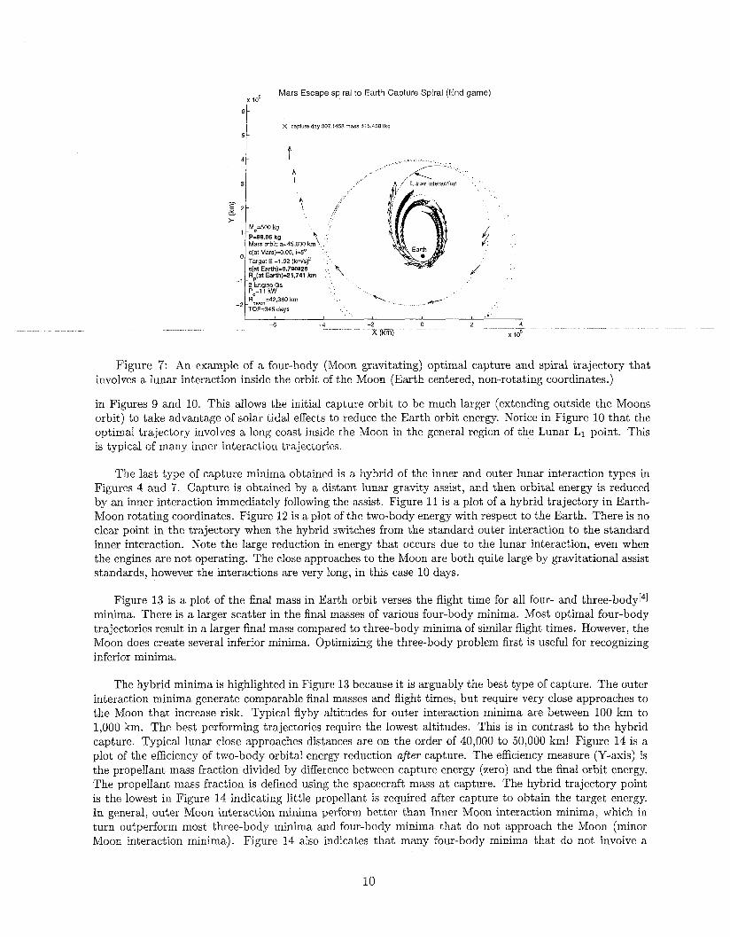
Figure 7: An example of a four-body (Moon gravitating) optimal capture and spiral trajectory that involves a lunar interaction inside the orbit of the Moon (Earth centered, non-rotating coordinates.)

in Figures 9 and 10. This allows the initial capture orbit to be much larger (extending outside the Moons orbit) to take advantage of solar tidal effects to reduce the Earth orbit energy. Notice in Figure 10 that the optimal trajectory involves a long coast inside the Moon in the general region of the Lunar L1 point. This is typical of many inner interaction trajectories.

The last type of capture minima obtained is a hybrid of the inner and outer lunar interaction types in Figures 4 and 7. Capture is obtained by a distant lunar gravity assist, and then orbital energy is reduced by an inner interaction immediately following the assist. Figure 11 is a plot of a hybrid trajectory in Earth- Moon rotating coordinates. Figure 12 is a plot of the two-body energy with respect to the Earth. There is no clear point in the trajectory when the hybrid switches from the standard outer interaction to the standard inner interaction. Note the large reduction in energy that occurs due to the lunar interaction, even when the engines are not operating. The close approaches to the Moon are both quite large by gravitational assist standards, however the interactions are very long, in this case 10 days.

Figure 13 is a plot of the final mass in Earth orbit verses the flight time for all four- and three-bodyr4] minima. There is a larger scatter in the final masses of various four-body minima. Most optimal four-body trajectories result in a larger final mass compared to three-body minima of similar flight times. However, the Moon does create several inferior minima. Optimizing the three-body problem first is useful for recognizing inferior minima.

The hybrid minima is highlighted in Figure 13 because it is arguably the best type of capture. The outer interaction minima generate comparable final masses and flight times, but require very close approaches to the Moon that increase risk. Typical flyby altitudes for outer interaction minima are between 100 km to 1,000 km. The best performing trajectories require the lowest altitudes. This is in contrast to the hybrid capture. Typical lunar close approaches distances are on the order of 40,000 to 50,000 km! Figure 14 is a plot of the efficiency of two-body orbital energy reduction after capture. The efficiency measure (Y-axis) is the propellant mass fraction divided by difference between capture energy (zero) and the final orbit energy. The propellant mass fraction is defined using the spacecraft mass at capture. The hybrid trajectory point is the lowest in Figure 14 indicating little propellant is required after capture to obtain the target energy. In general, outer Moon interaction minima perform better than Inner Moon interaction minima, which in turn outperform most three-body minima and four-body minima that do not approach the Moon (minor Moon interaction minima). Figure 14 also indicates that many four-body minima that do not involve a

10

3

2 -

-3

-1 0 1 2 3 4 5 6 7 8 X (km) x io’

EarU-Mwn Rotaling Cwrdinates TOF = 357.5 days Me = 500 kg

- M, = 408.62 kg P = 31.38 kg Target orbital E = -1.4 (kmlsf

Caplureday331.0252 mass419.1534 kg

Figure 8: An example of a four-body (Moon gravitating) optimal capture and spiral trajectory that involves a lunar gravitational interaction inside the orbit of the Moon - with two lunar close approaches (Earth centered, Earth-Moon rotating coordinates).

-3

lo,Mars Orbit-Earth Capture: Inner Lunar Flyby, Second Earth Rev. Eanh-Sun Rotating Coordinates I

-

I -6 -4 -2 0 2 4

X (km) x lo5

Figure 9: An example of a trajectory that uses an inner interaction with the Moon on the second Earth orbit after capture (Earth centered, Earth - Sun rotating coordinates.)

11

,,mars Orbit-Earth Capture: Inner Lunar Flyby, Second Earth Rev. I Earth-Moon Rotating Coordinates

z. O - Y - >

-1

-2

0 -

h

g -1 -

v

> -2 -

-3 -

4-

1 -

-

-

-5 t -6 4 -2 0 2 4

x (km) x 10’

Figure 10: An example of a trajectory that uses an inner interaction with the Moon on the second Earth orbit after capture (Earth centered, Earth - Moon rotating coordinates.)

,,Mars Escape Spiral - Earth Capture End Game: Hybrid Capture Earth-Moon Rotating Coordinates

I capture day309.3833 mass417.3161kg

I I I

-3 , -2 -1 0 1 2 3 4 5

x (km) x IOS

Figure 11: An example of a four-body (Moon gravitating) optimal capture and spiral trajectory that involves a “hybrid” lunar interaction (Earth-Moon rotating coordinates.)

12

1 - - r W

38 Spiral - Earth Capture End Game: Hybrid Capture

Engineson m - Engines off

5 P - -1 -

-1.5

\ Target energy

-

-

Engines on c

. - - . - . - - . - . .

1 - I 312 314 316 318 320 322 324 326

Time (days past start) - ~~

Figure 12: Two-body orbital energy with respect to the Earth for the hybrid Earth capture.

close approach to the Moon pay a performance price to avoid the Moon. This is evidenced by the fact that minor Moon interaction minima (downward pointing triangles) are often found above three-body minima (squares and upward pointing triangles) in Figure 14. Figure 14 indicates that four-body minima with major Moon interactions arrive during “capture windows” spaced by the lunar period of 28 days. The first capture window is between 300 and 310 days after Mars departure. Optimal trajectories that capture outside the clumps (between 300 to 310 days and 330 to 338 days) are trajectories that are three-body minima, avoid the Moon (minor Moon interaction minima), or aze inner interaction minima that typically interact with the Moon on the second or third revolution of Earth after capture.

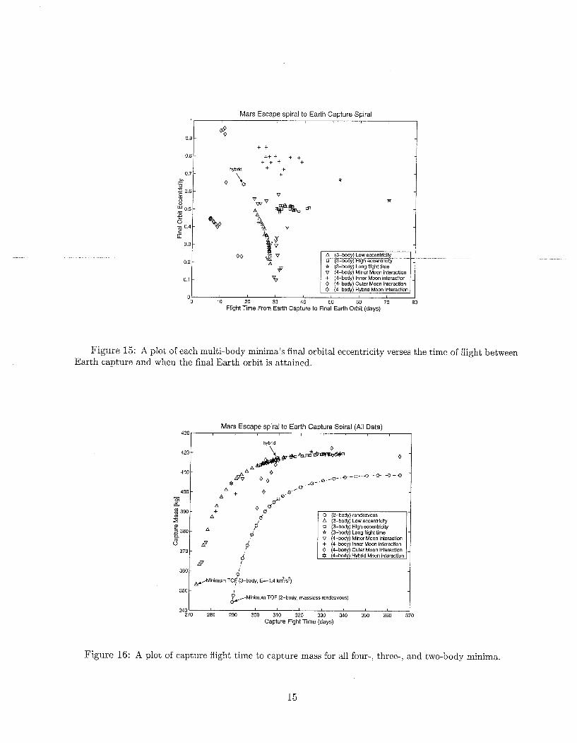
Figure 15 is a plot of the final eccentricity for all multi-body minima verses the time of flight from Earth capture to the iinai orbit. Ali trajectories in Figure 15 are constrained to a target final energy. The final eccentricity is optimized to maximize the delivered mass. Figure 15 indicates the eccentricity and flight time regimes that different optimal trajectory types tend to fall into. Outer interaction trajectories require short flight times after capture (around 10 days). Inner interaction trajectories have long flight times after capture (around 30 days) and usually end up with high eccentricity (around 0.75). Not unexpectedly, the hybrid sits in between the inner and outer interaction trajectories in both flight time and final eccentricity. Another feature of Figure 15 is that four-body solutions that do not come close to the Moon (downward pointing triangles) have longer flight times and more scatter than the corresponding three-body solutions (upward pointing triangles). This is consistent with the hypothesis that if the Moon is not approached closely (less than 100,000 km), then the Moon is actively avoided by the minima, and there is a performance cost relative to three-body solutions. When the Moon is avoided on the capture approach, the effect is an added acceleration roughly in the direction of Earth. Since the goal is to obtain a particular orbital energy with respect to the Earth, the acceleration due to the Moon will hurt performance.

Two-body capture can be optimized by treating the Earth and Moon as massless, and using the ren- dezvous Eq. (11). Figure 16 is a plot combining the two-, three-, and four-body local minima (ending the trajectories at capture). Figure 16 indicates that all multi-body minima outperform the corresponding two- body minima. The minimum feasible flight time to capture for the two-body problem is nearly 20 days longer than the minimum three-body flight time. Table 1 provides the improvement of multi-body optimization capture mass verses two-body optimization capture mass.

13

Mars Escape spiral to Earth Capture Spiral (E, =-I .4 km2/s2)

+A

A

360 _i an 350 t a

hybrid 0 0

A (3-body) Low eccentricity 0 (3-body) High eccentricity 0 (3-body) Long flight time v (4-body) No significant Moon interactior + (4-body) Inner type Moon interaction 0 (4-body) Outer type Moon interaction 0 (4-body) Hybrid type Moon interaction

1

Figure 13: Final mass in orbit verses total flight time is plotted for all four-body and three-body minima that are constrained to reach a final orbital energy of -1.4 $.

Mars Escape spiral to Earth Capture Spiral: Capture Spiral Efficiency

I I 0.04

V

I i VV

0 tc 4- . ._ - 2 0.015 - t + v)

4

E 0.01 00 0

a

I 0 -

3 A (3-bcdy) Low eccentricity 0 0 (3-body) High eccentricty

V (bbady) Minor Moon inieraoiion + (bbody) Inner Moan interaction 4 (4-body) Outer Moon interaction 0 (4-bcdy) Hybrid Moon interaction

- 4 / hybrid

O.Oo5 t (3-body) Longflighttime

280 290 300 310 320 Earth Capture [days past Mars departure]

Figure 14: A measure of the efficiency of the Earth spiral after capture. The propellant mass fraction is divided by the orbital energy reduction. For example, if the final target orbit has energy of -1.4 9, then the mass fraction of propellant used between the instant of capture (energy = 0) and when the final orbit is attained is divided by 1.4. The mass fraction is measured relative to the spacecraft mass at the instant of capture.

14

0 9 -

0 8 -

07- x t:

2 0 6 -

w 0 5 -

0 ~ i j 0 4 - c LL

a, 0

03-

~

0 2 -

0 1

Mars Escape spiral to Earth Capture Spiral

-

+ + +++ + + + + + t

hybrid + + +

n

00

B

*

*

t (3-body) Long flight time v (4-body) Minor Moon interaction + (4-body) Inner Moon interaction 0 (4-bodv) Outer Moon interaction I 0 &bod$) Hybrid Moon interaction I

0 10 20 30 40 50 60 70 80 Flight Time From Earth Capture to Final Earth Obit (days)

Figure 15: A plot of each multi-body minima's final orbital eccentricity verses the time of flight between Earth capture and when the final Earth orbit is attained.

Mars Escape spiral to Earth Capture Spiral (All Data) 430

hvbrid

420 t 0 &*4mi*E-=vw

$ 390 f A' d p'

B

d d

0 (2-body) rendezvous A (3-body) Low eccentricity 0 (3-body) High eccentricity t (3-body) Long flight time v (4-bodv) Minor Moon interaction

/ inhum TO? (3-body, E=-1.4 kn?/sz)

350 ?/inimum TOF (2-body, masslms rendezvous)

340 270 280 290 300 310 320 330 340 350 360 370

Capture Fight Time (days)

Figure 16: A plot of capture flight time to capture mass for all four-, three-, and two-body minima.

15

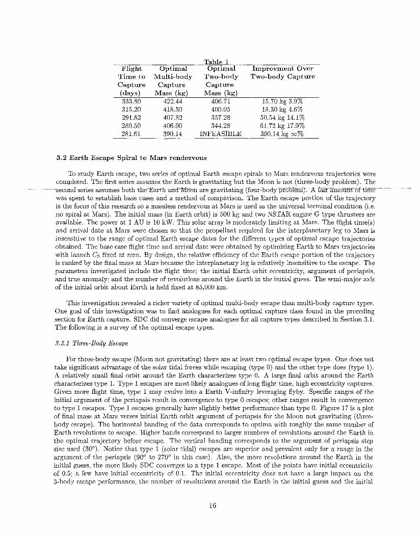
Flight Time to Capture

333.80 315.20 291.82 289.50 281.61

(days)

Table 1 Optimal Optimal Improvment Over

Multi- b ody Two- body Two- body Capture Capture Capture

Mass (kg) Mass (kg) 422.44 406.71 15.70 kg 3.9% 418.30 400.05 18.30 kg 4.6% 407.82 357.28 50.54 kg 14.1% 406.00 344.28 61.72 kg 17.9% 390.14 INFEASIBLE 390.14 ka 00%

3.2 Earth Escape Spiral to Mars rendezvous

To study Earth escape, two series of optimal Earth escape spirals to Mars rendezvous trajectories were completed. The first series assumes the Earth is gravitating but the Moon is not (three-body problem). The second series assumes both the Earth and Moon are gravitating (four-body problem). A fair amount of time was spent to establish base cases and a method of comparison. The Earth escape portion of the trajectory is the focus of this research so a massless rendezvous at Mars is used as the universal terminal condition (i.e. no spiral at Mars). The initial mass (in Earth orbit) is 500 kg and two NSTAR engine G type thrusters are available. The power at 1 AU is 10 kW. This solar array is moderately limiting at Mars. The flight time(s) and arrival date at Mars were chosen so that the propellant required for the interplanetary leg to Mars is insensitive to the range of optimal Earth escape dates for the different types of optimal escape trajectories obtained. The base case flight time and arrival date were obtained by optimizing Earth to Mars trajectories with launch Cz fixed at zero. By desigr,, the relative efficiency of the Earth esczpe portion of the trajectory is ranked by the final mass at Mars because the interplanetary leg is relatively insensitive to the escape. The parameters investigated include the flight time; the initial Earth orbit eccentricity, argument of periapsis, and true anomaly; and the number of revolutions around the Earth in the initial guess. The semi-major axis of the initial orbit about Earth is held fixed at 85,000 km.

This investigation revealed a richer variety of optimal multi-body escape than multi-body capture types. One goal of this investigation was to find analogues for each optimal capture class found in the preceding section for Earth capture. SDC did converge escape analogues for all capture types described in Section 3.1. The following is a survey of the optimal escape types.

3.2.1 Three-Body Escape

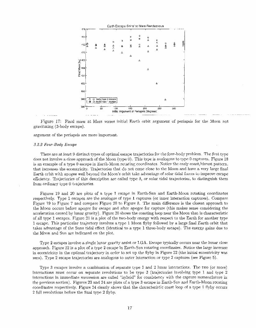
For three-body escape (Moon not gravitating) there are at least two optimal escape types. One does not take significant advantage of the solar tidal forces while escaping (type 0) and the other type does (type 1). A relatively small final orbit around the Earth characterizes type 0. A large final orbit around the Earth characterizes type 1. Type 1 escapes are most likely analogues of long flight time, high eccentricity captures. Given more flight time, type 1 may evolve into a Earth V-infinity leveraging flyby. Specific ranges of the initial argument of the periapsis result in convergence to type 0 escapes; other ranges result in convergence to type 1 escapes. Type 1 escapes generally have slightly better performance than type 0. Figure 17 is a plot of final mass at Mars verses initial Earth orbit argument of periapsis for the Moon not gravitating (three- body escape). The horizontal banding of the data corresponds to optima with roughly the same number of Earth revolutions to escape. Higher bands correspond to larger numbers of revolutions around the Earth in the optimal trajectory before escape. The vertical banding corresponds to the argument of periapsis step size used (30"). Notice that type 1 (solar tidal) escapes are superior and prevalent only for a range in the argument of the periapsis (90' to 270° in this case). Also, the more revolutions around the Earth in the initial guess, the more likely SDC converges to a type 1 escape. Most of the points have initial eccentricity of 0.5; a few have initial eccentricity of 0.1. The initial eccentricity does not have a large impact on the 3-body escape performance, the number of revolutions around the Earth in the initial guess and the initial

16

414

412

410

73408 Y

VI I

2 4 0 6 -

m

ii 404-

-

402

400

-

2 -

-

-

-

4 A

A (3-body) type 0 escape (3-body) type 1 escape

* A

A

0

A A A

o

h

A

0

0

8

0 0

0 A

0 0

A A

A

A

A

A

50 100 150 200 250 300 US”

Initial Argument of Periapsis [degrees] ~

Figure 17: Final mass at Mars verses initial Earth orbit argument of periapsis for the Moon not gravitating (3-body escape).

argument of the periapsis are more important.

3.2.2 Four-Body Escape

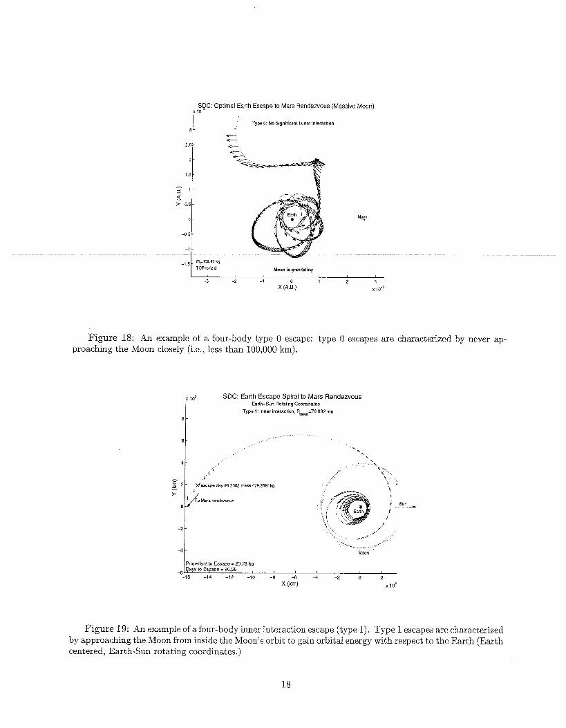
There are a t least 9 distinct types of optimal escape trajectories for the four-body problem. The first type does not involve a close approach of the Moon (type 0). This type is analogous to type 0 captures. Figure 18 is an example of a type 0 escape in Earth-Moon rotating coordinates. Notice the early coast/thrust pattern, that increases the eccentricity. Trajectories that do not come close to the Moon and have a very large final Earth crbit with apogee well beyond the Moon’s orbit take advantage of sohi tichi fu i~es to improve escape eEciency. Trajectories of this description are caiied type 8, or soiar tidai trajectories, to distinguish them from ordinary type 0 trajectories.

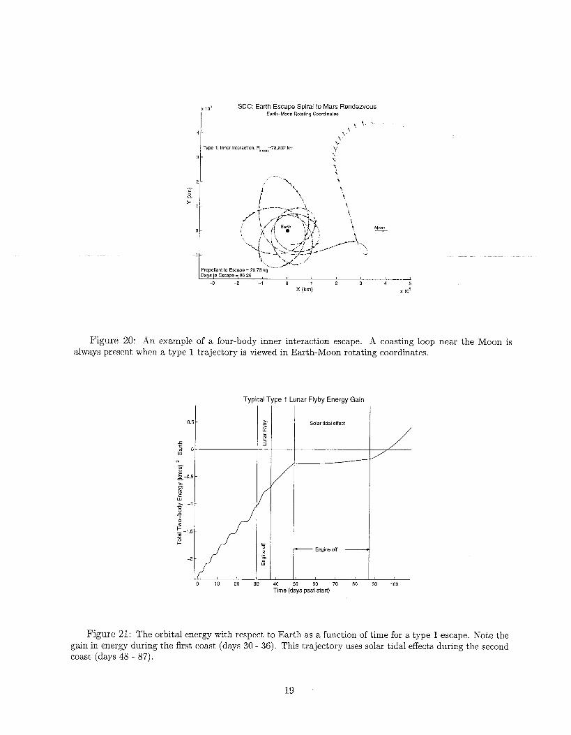
Figures 19 and 20 are plots of a type 1 escape in Earth-Sun and Earth-Moon rotating coordinates respectively. Type 1 escapes are the analogue of type 1 captures (or inner interaction captures). Compare Figure 19 to Figure 7 and compare Figure 20 to Figure 8. The main difference is the closest approach to the Moon occurs before apogee for escape and after apogee for capture (this makes sense considering the acceleration caused by lunar gravity). Figure 20 shows the coasting loop near the Moon that is characteristic of all type 1 escapes. Figure 21 is a plot of the two-body energy with respect to the Earth for another type 1 escape. This particular trajectory involves a type 1 Moon flyby followed by a large final Earth orbit that takes advantage of the Suns tidal effect (identical to a type 1 three-body escape). The energy gains due to the Moon and Sun are indicated on the plot.

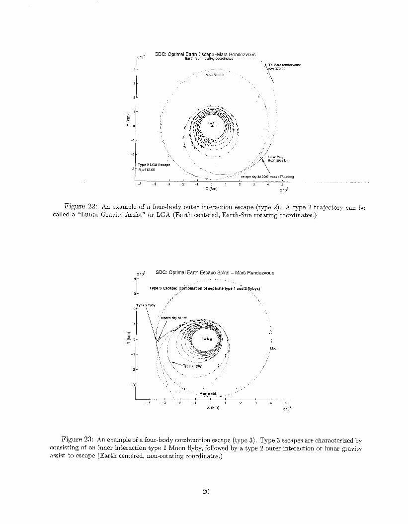
Type 2 escapes involve a single lunar gravity assist or LGA. Escape typically occurs near the lunar close approach. Figure 22 is a plot of a type 2 escape in Earth-Sun rotating coordinates. Notice the large increase in eccentricity in the optimal trajectory in order to set up the flyby in Figure 22 (the initial eccentricity was zero). Type 2 escape trajectories are analogous to outer interaction or type 2 captures (see Figure 5 ) .

Type 3 escapes involve a combination of separate type 1 and 2 lunar interactions. The two (or more) interactions must occur on separate revolutions to be type 3 (trajectories involving type 1 and type 2 interactions in immediate succession are called “hybrid” for consistency with the capture nomenclature in the previous section). Figures 23 and 24 are plots of a type 3 escape in Earth-Sun and Earth-Moon rotating coordinates respectively. Figure 24 clearly shows that the characteristic coast loop of a type 1 flyby occurs 2 full revolutions before the final type 2 flyby.

17

3 -

2.5

Type 0: No Significant Lunar Interaction

c t.

- & -

-l,5t Mg.409.92kg TOF372 d Moan is gravitating

1 5 -

- 3 1 - s > 0 5 -

0 -

-0 5

-1 ~

I , -3 -2 -1 0 1 2 3

X (A.U.) x 10.’

2 -

-

-

Figure 18: An example of a four-body type 0 escape: type 0 escapes are characterized by never ap- proaching the Moon closely (Le., less than 100,000 km).

Propellant to Escape = 20.73 kg

SDC: Earth Escape Spiral to Mars Rendezvous Earth-Sun Rotating Coordinates

Type 1: Inner interaction, Rman=78,832 km

>oi ‘/a Mars rendezvous

4 -*I MOO”

Figure 19: An example of afour-body inner interaction escape (type 1). Type 1 escapes are characterized by approaching the Moon from inside the Moon’s orbit to gain orbital energy with respect to the Earth (Earth centered, Earth-Sun rotating coordinates.)

18

SDC: Earth Escape Spiral to Mars Rendezvous Earlh-Mwn Rotating Coordinates

\ \ ‘ *

4 r \ \:,

Type 1: Inner interaction, RmWn=78,832 km \: 9 k

I Y

Figure 20: An example of a four-body inner interaction escape. A coasting loop near the Moon is always present when a type 1 trajectory is viewed in Earth-Moon rotating coordinates.

Typical Type 1 Lunar Flyby Energy Gain

Figure 21: The orbital energy with respect to Earth as a function of time for a type 1 escape. Note the gain in energy during the first coast (days 30 - 36). This trajectory uses solar tidal effects during the second coast (days 48 - 87).

19

SDC: Optimal Earth Escape-Mars Rendezvous Eaflh-Sun rotating coordinates

To Mars rendezvous

Moon's orbit

Figure 22: An example of a four-body outer interaction escape (type 2). A type 2 trajectory can be called a "Lunar Gravity Assist" or LGA (Earth centered, Earth-Sun rotating coordinates.)

ro5 SDC: Optimal Earth Escape Spiral - Mars Rendezvous

I Type 3 Escape: (combination of separate type 1 and 2 flybys)

Figure 23: An example of a four-body combination escape (type 3 ) . Type 3 escapes are characterized by consisting of an inner interaction type 1 Moon flyby, followed by a type 2 outer interaction or lunar gravity assist to escape (Earth centered, non-rotating coordinates.)

20

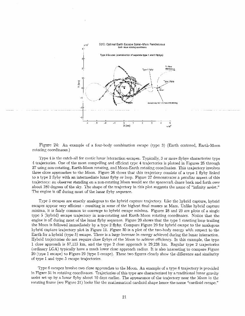
SDC: Optimal Earth Escape Spiral-Mars Rendezvous Earlh-Moon rotating cwrdinates

Type 3 Escape: (combination of separate type 1 and 2 flybys)

-3 t I ,

- 4 - 3 - 2 - 1 0 1 2 3 4 5

X (km) x 10’

Figure 24: An example of a four-body combination escape (type 3) (Earth centered, Earth-Moon rotating coordinates.)

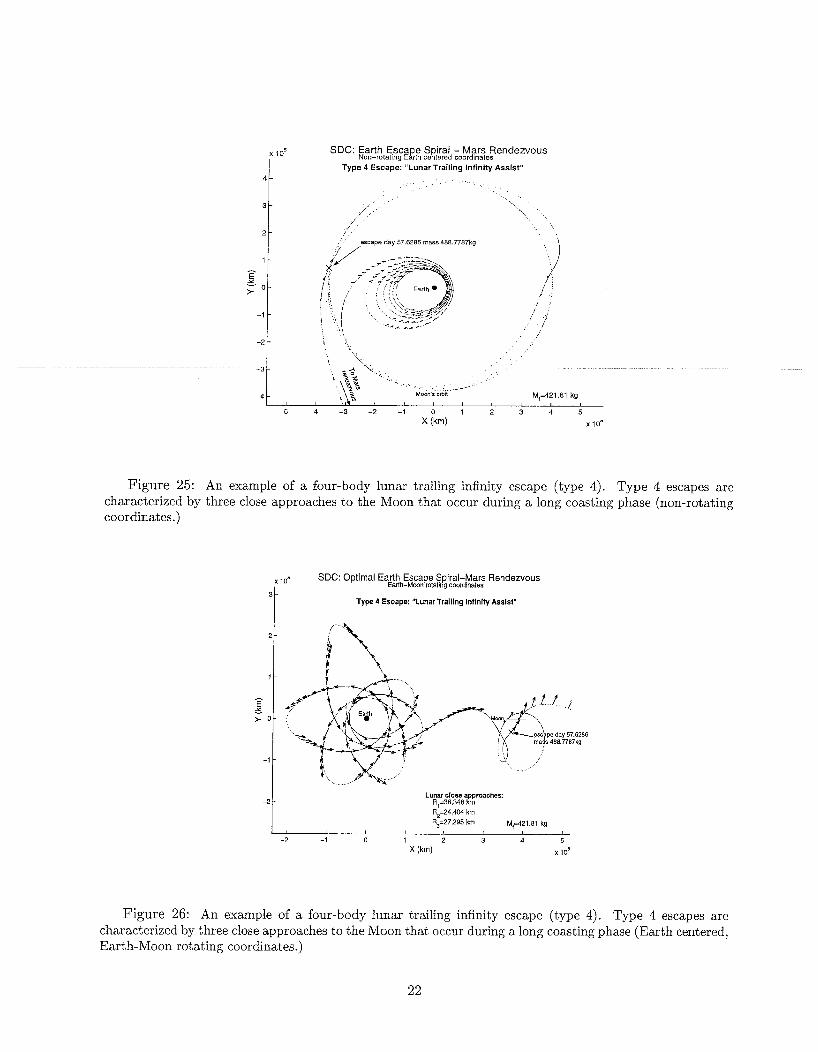
Type 4 is the catch-all for exotic lunar interaction escapes. Typically, 3 or more flybys characterize type 4 trajectories. One of the most compelling and efficient type 4 trajectories is plotted in Figures 25 through 27 using non-rotating, Earih-Moon rotaiiiig, alld Mooil-Ealth lotdiirig wurdiuaies. This i ra jectay involves three close approaches to the Moon. Figure 26 shows that this trajectory consists of a type 1 flyby linked to a type 2 flyby with an intermediate lunar flyby or loop. Figure 27 demonstrates a peculiar aspect of this trajectory: an observer standing on a non-rotating Moon would see the spacecraft dance back and forth over about 180 degrees of the sky. The shape of the trajectory in this plot suggests the name of “infinity assist.” The engine is off during most of the lunar flyby sequence.

Type 5 escapes are exactly analogous to the hybrid capture trajectory. Like the hybrid capture, hybrid escapes appear very efficient - resulting in some of the highest final masses at Mars. Unlike hybrid capture minima, it is fairly common to converge to hybrid escape minima. Figures 28 and 29 are plots of a single type 5 (hybrid) escape trajectory in non-rotating and Earth-Moon rotating coordinates. Notice that the engine is off during most of the lunar flyby sequence. Figure 29 shows that the type 1 coasting loop trailing the Moon is followed immediately by a type 2 flyby. Compare Figure 29 for hybrid escape t o the analogous hybrid capture trajectory plot in Figure 11. Figure 30 is a plot of the two-body energy with respect to the Earth for a hybrid (type 5) escape. There is a large increase in energy achieved during the lunar interaction. Hybrid trajectories do not require close flybys of the Moon to achieve efficiency. In this example, the type 1 close approach is 57,115 km, and the type 2 close approach is 29,238 km. Regular type 2 trajectories (ordinary LGA) typically have a much lower close approach radius. It is also interesting to compare Figure 20 (type 1 escape) to Figure 29 (type 5 escape). These two figures clearly show the difference and similarity of type 1 and type 5 escape trajectories.

Type 6 escapes involve two close approaches to the Moon. An example of a type 6 trajectory is provided in Figure 31 in rotating coordinates. Trajectories of this type are characterized by a traditional lunar gravity assist set up by a lunar flyby about 10 days earlier. The appearance of the trajectory near the Moon in the rotating frame (see Figure 31) looks like the mathematical cardioid shape hence the name “cardioid escape.”

21

3 -

2-

1 - - E 5 0-

-1 -

,/' scape day 57.6286 mass 488.7787kg

Figure 25: An example of a four-body lunar trailing infinity escape (type 4). Type 4 escapes are characterized by three close approaches to the Moon that occur during a iong coasting phase (non-rotating coordinates .)

SDC: Optimal Earth Escape Spiral-Mars Rendezvous Earih-Moon rotating coordinates

Type 4 Escape: "Lunar Trailing Infinity Assist"

Lunar close approaches: R,=38,348 km R2=24,404 km

R,=27,295 km M,=421.81 kg

-2 -1 0 1 2 3 4 5

X (km) x 10'

Figure 26: An example of a four-body lunar trailing infinity escape (type 4). Type 4 escapes are characterized by three close approaches to the Moon that occur during a long coasting phase (Earth centered, Earth-Moon rotating coordinates.)

22

3 -

2 -

1 -

0 - - E

2. -1 Y -

-2

-3

4-

SDC: Optimal Earth Escape Spiral - Mars Rendezvous NON-ROTATING Moon centered coardinates

Type 4 Escape: 'Lunar Trailing Infinity Assist" - -\ 4 -

-

- -

-5

-6

Figure 27: An example of a four-body lunar trailing infinity escape (type 4). In Moon centered, non- rotating coordinates, the trajectory has a characteristic infinity symbol shape, trailing the Moon.

Lunar close approaches: . < * - - - R1=38,348 km 3"

R2=24.404 km C P 32 , $?E , M,=421 81 kg - R3=27,295 km

105 SDC: Earth Escape to Mars Rendezvous: "The Hybrid"

M0=500 kg Ml=422 68 kg

TOF=372 d

Mwn's Oiblt

I. . .

. . ,/ .: This escape is an analogue to the Hybrid

Capture I discovered (please see Figure 15: i , . : Summaryof Work5.16.01).

-

-1 !I -2

. , Escape day 57.2 mass 489.94 kg

. .

1

,'. -Type 1 flyby . . , . R57,115 km To Mars

-4 -3 -2 -1 0 1 2 3 4

X ikm) x105

Figure 28: An example of a four-body hybrid escape (type 5). Type 5 escapes are characterized by two close approaches to the Moon. Hybrid escapes are the analogue of hybrid captures (non-rotating coordinates.)

23

SDC: Optimal Earth Escape to Mars Rendezvous "The Hybrid Earth-Moon rotating coordinates

-2

R=29 238 km

, ...' - "- '.' Me==500 kg M,=422.68 kg

TOFd72 d 1

94 kg

Figure 29: An example of a four-body hybrid escape (type 5) (Earth-Moon rotating coordinates.)

SDC: Optimal Earth Escape to Mars Rendezvous "The Hybrid"

Figure 30: An example of the orbital energy with respect to Earth verses time for a hybrid escape (type 5 ) . Hybrid trajectories achieve a significant increase in energy during coasting near the Moon.

24

SDC: Optimal Earth Escape Spiral to Mars Rendezvous: Cardioid Escape Earth-Mm Rotating Cwrdinates

1 -

- 0

g - >

-1

-2

Fiyby 1: R=12,413 km

i[ -

=ape day 58.142 mass 483.2972kg

-

M,=419.34 kg TOFS72 d

Type 6

Figure 31: An example of a four-body cardiod escape (type 6). In Earth centered, Earth-Moon rotating coordinates, the trajectory near the Moon has the appearance of the mathematical cardiod shape.

Four trajectories of this type resulted from different initial Earth orbit conditions

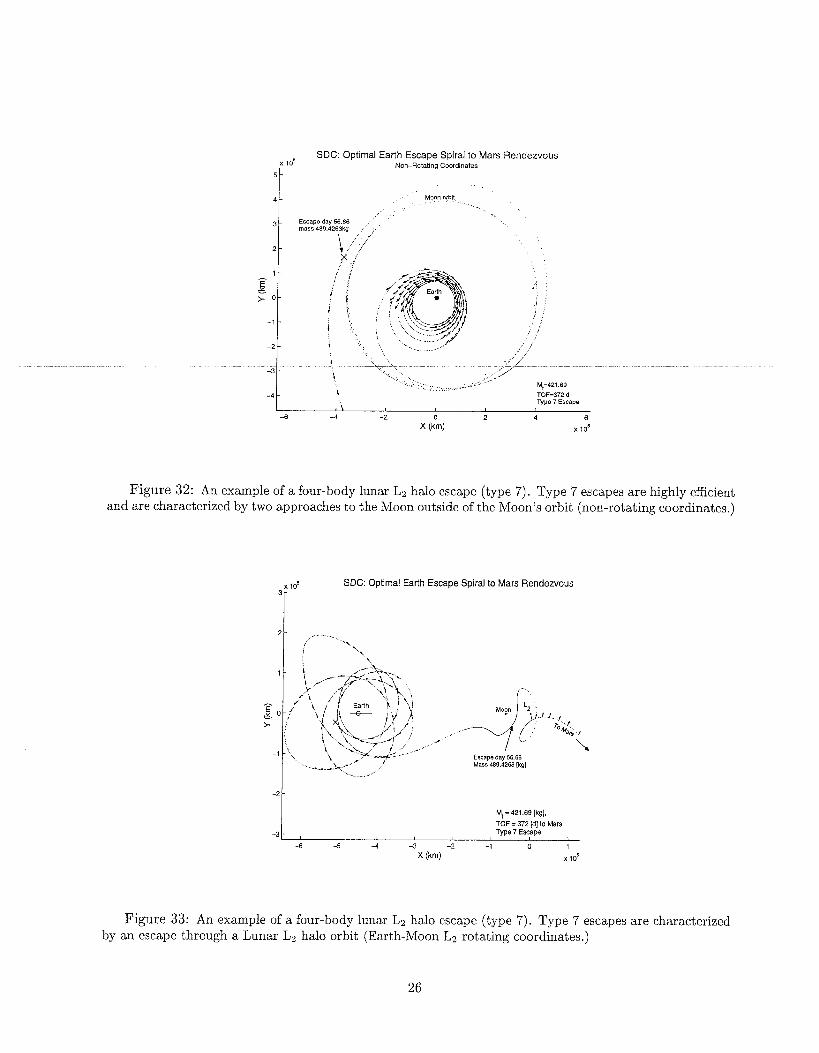
Type 7 escapes involve two close approaches to the Moon during a long coasting phase. An example of a type 7 trajectory is provided in Figures 32 and 33. Trajectories of this type are characterized by a single revolution around a lunar L2 halo orbit. This trajectory is very efficient, comparable to the hybrid class (type 5). This trajectory was named “lunar L2 halo” escape because of the halo orbit. Many trajectories of this type were obtained - it proved to be easy to construct an initial guess trajectory that will converge to this type of trajectory.

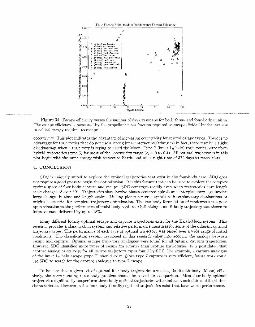
Figure 34 is a plot of escape efficiency verses the number of days to escape for both three- and four-body minima. The escape efficiency is measured by the propellant mass fraction required to escape divided by the increase in orbital energy required to escape. All initial orbits begin with an energy of -2.3447 so the mass fraction is divided by 2.3447. This definition of escape efficiency is the analouge of the capture efficiency plotted in Figure 14. The overall winner (lower is better) is a lunar Lz halo escape trajectory (type 7). The second best is a hybrid (type 5). Close behind is a lunar 03 assist (type 4). All three benefit from high initial Earth orbit eccentricities. Notice that the best four-body performers (and a wide variety of types) all escape somewhere in a very small escape date window (around 56 to 57 days). This time must be ideal for getting a lunar assist to go on to Mars. Not surprisingly, the type 0 three-body minima use as much time as possible to escape (around 95 days.) Escape times in excess of 95 days begin to significantly degrade the interplanetary leg performance.

Comparing escape efficiency (Figure 34) to capture efficiency (Figure 14) provides several insights, Four- body escape efficiency is essentially the same as four-body capture efficiency as measured in Figures 34 and 14. This result is consistent with the idea that optimal capture trajectories have analogous optimal escape trajectories. SDC did not locate capture analogues for all of the escape types. For example, no capture analogue was found for the lunar L2 halo escapes (type 7). This does not mean that type 7 captures do not exist, only that the region of influence of type 7 captures may be small or do not exist for incoming energy much greater than zero. Three-body escape is a little more efficient than the corresponding three-body capture. This difference probably reflects the difference in the phasing and geometry of the interplanetary trajectory, not an inherent difference between three-body capture and escape.

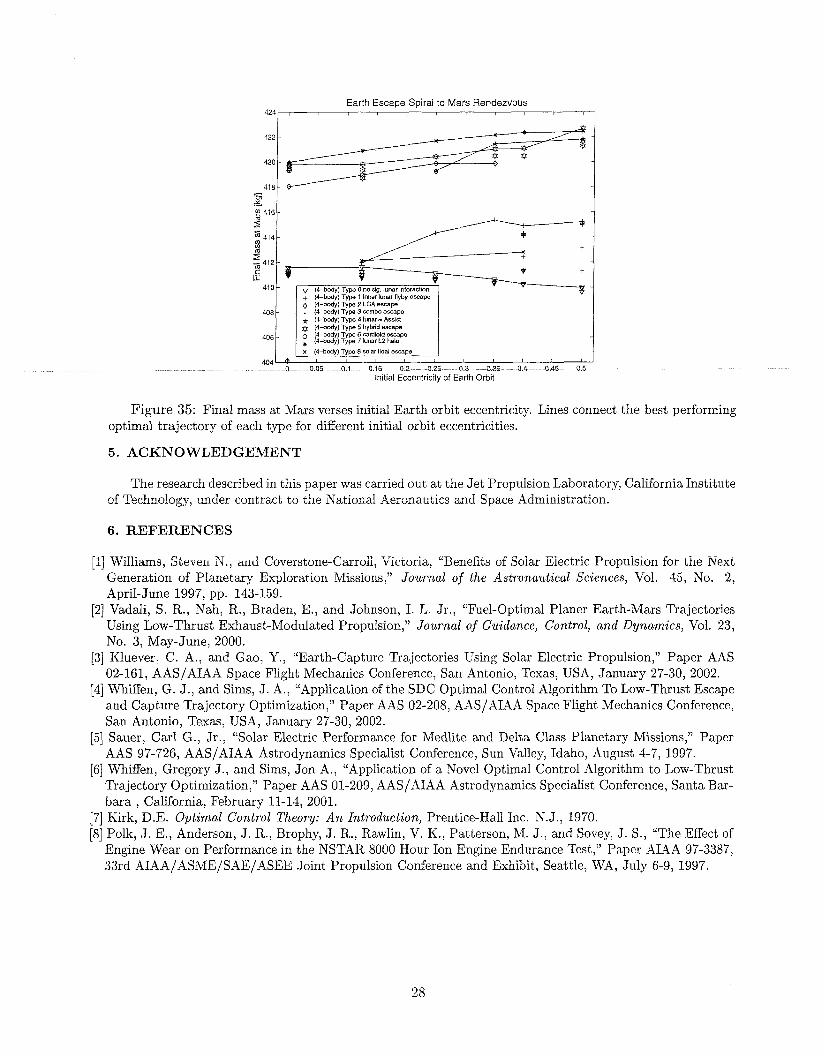
Quantifying the effect of initial Earth orbit eccentricity on performance is important for designing to the Earth orbit used in this research. Figure 35 is a plot of final mass at Mars verses the initial Earth orbit

25

SDC: Optimal Earth Escape Spiral to Mars Rendezvous x 10’ Non-Rotating Coordinates

3-

Figure 32: An example of a four-body lunar L2 halo escape (type 7). Type 7 escapes are highly efficient and are characterized by two approaches to the Moon outside of the Moon’s orbit (non-rotating coordinates.)

M,=421.69 [kg],

TOF = 372 [d] to Mars I Type 7 Escape

SDC: Optimal Earth Escape Spiral to Mars Rendezvous 3r .-

Escape day 56.66 Mass 489.4263 [kgl

-2 t

Figure 33: An example of a four-body lunar Lz halo escape (type 7). Type 7 escapes are characterized by an escape through a Lunar La halo orbit (Earth-Moon L2 rotating coordinates.)

26

Earth Escape Spiral to Mars Rendezvous: Escape Efficiency

g 0.022 *,. *- 1 -

A 0

V + 0

A A

A

(I-body) type 0 escape (3-body) type 1 escape (4-body) Type 0 WEak iunar (4-body) Type 1 inner lunar (bbody) Type 2 LGA escape (4-body) Type 3 combo (4-body) Type 4 iunar- Assid (4-body) Type 5 hybrid (4-body1 Type 6 oardiaid (4-body) Type 7 iunar L2 halo (4-body) Type 8 soia tidal

B 0.012

g 0.01 a z l

A

A 0

0 o *

8

0

Days to Escape

Figure 34: Escape efficiency verses the number of days to escape for both three- and four-body minima. The escape efficiency is measured by the propellant mass fraction required to escape divided by the increase in orbital energy required to escape.

eccentricity. This plot indicates the advantage of increasing eccentricity for several escape types. There is no advantage for trajectories that do not use a strong lunar interaction (triangles) in fact, there may be a slight disadvantage when a trajectory is trying to avoid the Moon. Type 7 (lunar L2 halo) trajectories outperform hybrid trajectories (type 5 ) for most of the eccentricity range (Q = 0 to 0.4), All optimal trajectories in this plot begin with the same energy with respect to Earth, and use a flight time of 372 days to reach Mars.

4. CONCLUSION

SDC is uniquely suited to explore the optimal trajectories that exist in the four-body case. SDC does not require a good guess to begin the optimization. It is this feature that can be used to explore the complex optima space of four-body capture and escape. SDC converges readily even when trajectories have length scale changes of over lo4. Trajectories that involve planet centered spirals and interplanetary legs involve large changes in time and length scales. Linking planet centered spirals to interplanetary destinations or origins is essential for complete trajectory optimization. The two-body formulation of rendezvous is a poor approximation to the performance of multi-body capture. Optimizing a multi-body trajectory was shown to improve mass delivered by up to 18%.

Many different locally optimal escape and capture trajectories exist for the Earth-Moon system. This research provides a classification system and relative performance measures for some of the different optimal trajectory types. The performance of each type of optimal trajectory was tested over a wide range of initial conditions. The classification system developed in this research takes into account the analogy between escape and capture. Optimal escape trajectory analogues were found for all optimal capture trajectories. However, SDC identified more types of escape trajectories than capture trajectories. It is postulated that capture analogues do exist for all escape trajectory types found by SDC. For example, a capture analogue of the lunar Lz halo escape (type 7) should exist. Since type 7 capture is very efficient, future work could use SDC to search for the capture analogue to type 7 escape.

To be sure that a given set of optimal four-body trajectories are using the fourth body (Moon) effec- tively, the corresponding three-body problem should be solved for comparison. Most four-body optimal trajectories significantly outperform three-body optimal trajectories with similar launch date and flight time characteristics. However, a few four-body (locally) optimal trajectories exist that have worse performance.

27

Earth Escape Spiral to Mars Rendezvous 424 I

2 1 Y2 416

2 z 4 1 4 -

I - 412 - li

2

E 410 -

408 -

406 -

404 -

v + V

+ (4-body) Type 1 lnnerlunarflyby escape Q (4-body) Type 2 LGA escape

(4-body) Type 3 combo escape * (4-body) Type 4 lunar- Assst (4-body) Type 5 hybnd escape (4-body) Type 6 cardioid escape (4-body) Type 7 lunar L2 halo *i

0 005 0.1 015 -02 ~ 0 2 5 0 3 4 3 5 0 4 0 4 5 0 5 initial Eccentricity of Earth Orbit

Figure 35: Final mass at Mars verses initial Earth orbit eccentricity. Lines connect the best performing optimal trajectory of each type for different initial orbit eccentricities.

5 . A C K N O W L E D G E M E N T

The research described in this paper was carried out a t the Jet Propulsion Laboratory, California Institute of Technology, under cmtract tc the National Aeronautics and Space Administration.

6 . REFERENCES

[I] Williams, Steven N., aid Coverstone-Carroll, Victoria, “Benefits of Solar Electric Propulsion for the Next Generation of Planetary Exploration Missions,’’ Journal of the Astronautical Sciences, Vol. 45, No. 2, April-June 1997, pp. 143-159.

[2] Vadali, S. R., Nah, R., Braden, E., and Johnson, I. L. Jr., “Fuel-Optimal Planer Earth-Mars Trajectories Using Low-Thrust Exhaust-Modulated Propulsion,” Journal of Guidance, Control, and Dynamics, Vol. 23, No. 3, May-June, 2000.

[3] Kluever, C. A., and Gao, Y., “Earth-Capture Trajectories Using Solar Electric Propulsion,” Paper AAS 02-161, AAS/AIAA Space Flight Mechanics Conference, San Antonio, Texas, USA, January 27-30, 2002.

[4] Whiffen, G. J . , and Sims, J. A., “Application of the SDC Optimal Control Algorithm To Low-Thrust Escape and Capture Trajectory Optimization,” Paper AAS 02-208, AAS/AIAA Space Flight Mechanics Conference, San Antonio, Texas, USA, January 27-30, 2002.

[5] Sauer, Carl G., Jr., “Solar Electric Performance for Medlite and Delta Class Planetary Missions,” Paper AAS 97-726, AAS/AIAA Astrodynamics Specialist Conference, Sun Valley, Idaho, August 4-7, 1997.

[6] Whiffen, Gregory J., and Sims, Jon A., “Application of a Novel Optimal Control Algorithm to Low-Thrust Trajectory Optimization,” Paper AAS 01-209, AAS/AIAA Astrodynamics Specialist Conference, Santa Bar- ba ra , California, February 11-14, 2001.

[7] Kirk, D.E. Optimal Control Theory: An Introduction, Prentice-Hall Inc. N. J., 1970. [8] Polk, J . E., Anderson, J. R., Brophy, J . R., Rawlin, V. K., Patterson, M. J., and Sovey, J . S., “The Effect of

Engine Wear on Performance in the NSTAR 8000 Hour Ion Engine Endurance Test,” Paper AIAA 97-3387, 33rd AIAA/ASME/SAE/ASEE Joint Propulsion Conference and Exhibit, Seattle, WA, July 6-9, 1997.

28