Application of SWAT Model to an Agricultural Watershed in ... · 1Assistant Professor, 2PG Student and 3Professor ... [email protected] Centre for Water Resources Anna University,

Application of SWAT Model to an AgriculturalWatershed in Tamil Nadu, India

2012 International SWAT Conference, 18 - 20 July, 2012

Arun Babu Elangovan1, Suresh P2 and Ravichandran Seetharaman3

1Assistant Professor, 2PG Student and 3ProfessorE Mail: [email protected]

Centre for Water ResourcesAnna University, Chennai -600025Tamil Nadu, India

Outline

• Introduction• Study Area• Preparation of Data Sets• Model parameterization• SWAT Run• SWAT CUP• Sensitivity Analysis• Results

• Introduction• Study Area• Preparation of Data Sets• Model parameterization• SWAT Run• SWAT CUP• Sensitivity Analysis• Results

7/18/2012 2012 SWAT Conference 2

Introduction

• Water is the most important natural resource

• Current Scenario: Scarcity of fresh water, vulnerability

of the available resources, shift in the rainfall pattern,

climate change, eutrophication etc

• Need of the hour is to create a strategy and identify

tools to model the watershed

• SWAT – Open source, worldwide usage

• Water is the most important natural resource

• Current Scenario: Scarcity of fresh water, vulnerability

of the available resources, shift in the rainfall pattern,

climate change, eutrophication etc

• Need of the hour is to create a strategy and identify

tools to model the watershed

• SWAT – Open source, worldwide usage


Context of the Study

• Application of SWAT model to this study watershed

is a first attempt

• Study the possibility and the adaptability of SWAT

model to depict the functionality of the watershed

• Preliminary results of the model is presented(needs

further improvement)

• Application of SWAT model to this study watershed

is a first attempt

• Study the possibility and the adaptability of SWAT

model to depict the functionality of the watershed

• Preliminary results of the model is presented(needs

further improvement)


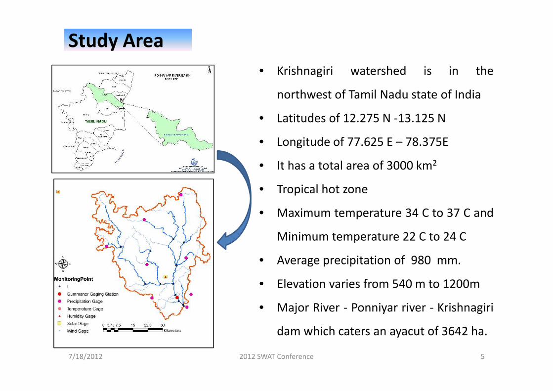
Study Area• Krishnagiri watershed is in the

northwest of Tamil Nadu state of India

• Latitudes of 12.275 N -13.125 N

• Longitude of 77.625 E – 78.375E

• It has a total area of 3000 km2

• Tropical hot zone

• Maximum temperature 34 C to 37 C and

Minimum temperature 22 C to 24 C

• Average precipitation of 980 mm.

• Elevation varies from 540 m to 1200m

• Major River - Ponniyar river - Krishnagiri

dam which caters an ayacut of 3642 ha.

• Krishnagiri watershed is in the

northwest of Tamil Nadu state of India

• Latitudes of 12.275 N -13.125 N

• Longitude of 77.625 E – 78.375E

• It has a total area of 3000 km2

• Tropical hot zone

• Maximum temperature 34 C to 37 C and

Minimum temperature 22 C to 24 C

• Average precipitation of 980 mm.

• Elevation varies from 540 m to 1200m

• Major River - Ponniyar river - Krishnagiri

dam which caters an ayacut of 3642 ha.


Preparation of Datasets

• DEM - SRTM 90 m resolution

• Landuse - Resourcesat Image

• Soil - Agricultural Engineering

Department + Soil samplings

• Climate - FCS at two locations

• Rainfall - Raingauges at eight locations

• Discharge - At one location (CWC)

• Sediment - At one location (CWC)

• Time line - 1998 – 2000 (Warmup)

2001 – 2005 (calibration)

2006 – 2010 (validation)

• DEM - SRTM 90 m resolution

• Landuse - Resourcesat Image

• Soil - Agricultural Engineering

Department + Soil samplings

• Climate - FCS at two locations

• Rainfall - Raingauges at eight locations

• Discharge - At one location (CWC)

• Sediment - At one location (CWC)

• Time line - 1998 – 2000 (Warmup)

2001 – 2005 (calibration)

2006 – 2010 (validation)


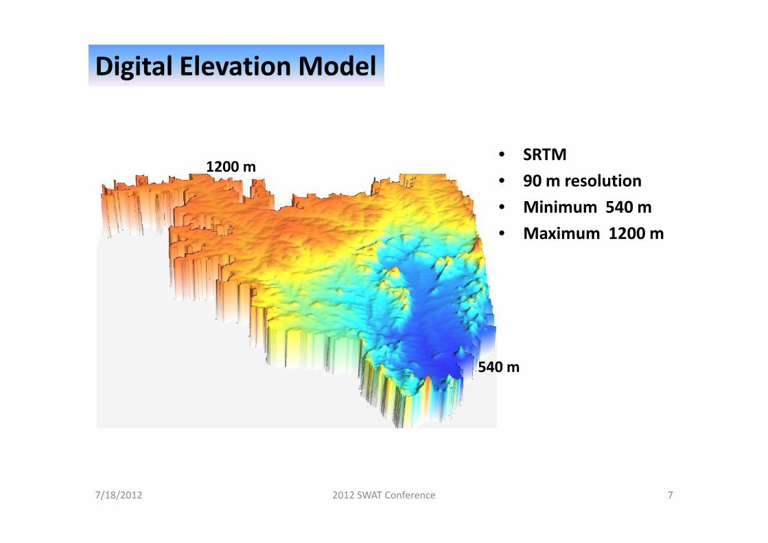
Digital Elevation Model

• SRTM• 90 m resolution• Minimum 540 m• Maximum 1200 m

1200 m


540 m

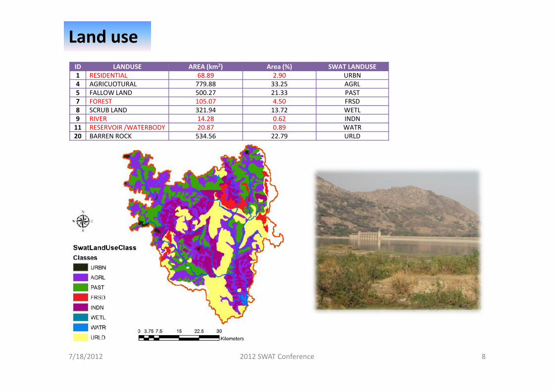
Land useID LANDUSE AREA (km2) Area (%) SWAT LANDUSE1 RESIDENTIAL 68.89 2.90 URBN4 AGRICUOTURAL 779.88 33.25 AGRL5 FALLOW LAND 500.27 21.33 PAST7 FOREST 105.07 4.50 FRSD8 SCRUB LAND 321.94 13.72 WETL9 RIVER 14.28 0.62 INDN

11 RESERVOIR /WATERBODY 20.87 0.89 WATR20 BARREN ROCK 534.56 22.79 URLD


SoilID SOIL SERIES AREA

(km2) Area (%) SWAT SOIL CLASSIFICATION(USER SOIL GROUP)

1 KELAMANGALAM SERIES 214 9.49 KELAMANGALAM SERIES2 ROCKOUTCROP 287 12.60 ROCKOUTCROP3 VANNAPATTI SERIES 400 17.46 VANNAPATTI SERIES4 KRISHNAGIRI SERIES 17 0.84 KRISHNAGIRI SERIES5 HOSUR SERIES 775 29.97 HOSUR SERIES6 SONEPURAM SERIES 722 29.64 SONEPURAM SERIES


Rain gauge , Flow gauge and Weather station

• 8 Rain gauges

• 1 Flow gauge

• 2 weather station

• Temporal resolution of

data: daily measurements

• (used monthly flow data

for preliminary analysis)


• 8 Rain gauges

• 1 Flow gauge

• 2 weather station

• Temporal resolution of

data: daily measurements

• (used monthly flow data

for preliminary analysis)

•Preprocessors were used to generate the weather statistics•User weather database has been created•Preprocessors were used to generate the weather statistics•User weather database has been created

Model Setup

• Arc SWAT 2009 interfaced with ArcGIS 9.3

• 26 subbasins (using DEM +Gauges)

• 417 HRUS by using multiple Landuse / Soil

/Slope (THRESHOLDS : 5 / 5 / 5 [%])

• 8 years data were used to run the model

(NYSKIP = 3)

• 1998 – 2000 (Warmup)

• 2001 – 2005 (simulated in ArcSWAT)

• Output in Txtinout folder


• Arc SWAT 2009 interfaced with ArcGIS 9.3

• 26 subbasins (using DEM +Gauges)

• 417 HRUS by using multiple Landuse / Soil

/Slope (THRESHOLDS : 5 / 5 / 5 [%])

• 8 years data were used to run the model

(NYSKIP = 3)

• 1998 – 2000 (Warmup)

• 2001 – 2005 (simulated in ArcSWAT)

• Output in Txtinout folder

Calibration : SWAT- CUP (Calibration and Uncertainity Programs)

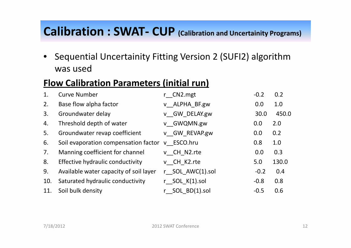
• Sequential Uncertainity Fitting Version 2 (SUFI2) algorithmwas used

Flow Calibration Parameters (initial run)1. Curve Number r__CN2.mgt -0.2 0.22. Base flow alpha factor v__ALPHA_BF.gw 0.0 1.03. Groundwater delay v__GW_DELAY.gw 30.0 450.04. Threshold depth of water v__GWQMN.gw 0.0 2.05. Groundwater revap coefficient v__GW_REVAP.gw 0.0 0.26. Soil evaporation compensation factor v__ESCO.hru 0.8 1.07. Manning coefficient for channel v__CH_N2.rte 0.0 0.38. Effective hydraulic conductivity v__CH_K2.rte 5.0 130.09. Available water capacity of soil layer r__SOL_AWC(1).sol -0.2 0.410. Saturated hydraulic conductivity r__SOL_K(1).sol -0.8 0.811. Soil bulk density r__SOL_BD(1).sol -0.5 0.6

• Sequential Uncertainity Fitting Version 2 (SUFI2) algorithmwas used

Flow Calibration Parameters (initial run)1. Curve Number r__CN2.mgt -0.2 0.22. Base flow alpha factor v__ALPHA_BF.gw 0.0 1.03. Groundwater delay v__GW_DELAY.gw 30.0 450.04. Threshold depth of water v__GWQMN.gw 0.0 2.05. Groundwater revap coefficient v__GW_REVAP.gw 0.0 0.26. Soil evaporation compensation factor v__ESCO.hru 0.8 1.07. Manning coefficient for channel v__CH_N2.rte 0.0 0.38. Effective hydraulic conductivity v__CH_K2.rte 5.0 130.09. Available water capacity of soil layer r__SOL_AWC(1).sol -0.2 0.410. Saturated hydraulic conductivity r__SOL_K(1).sol -0.8 0.811. Soil bulk density r__SOL_BD(1).sol -0.5 0.6


Initial Run - Results


Variable p-factor r-factor R2 NS br2 MSE SSQRFLOW_OUT_21 0.25 0.07 0.60 0.04 0.0478 397377.8438 383871.8125

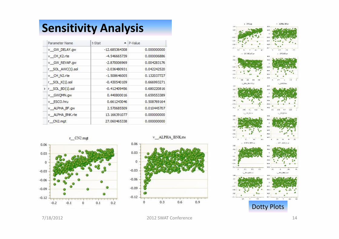
Sensitivity Analysis


Dotty Plots

Second Iteration

• Error in the peaks – uncertainity in precipitation• Limitation of climatic data, soil data


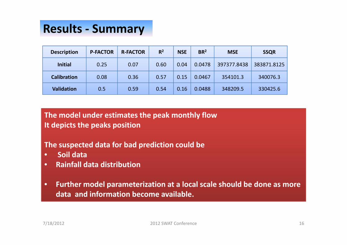
Results - SummaryDescription P-FACTOR R-FACTOR R2 NSE BR2 MSE SSQR

Initial 0.25 0.07 0.60 0.04 0.0478 397377.8438 383871.8125

Calibration 0.08 0.36 0.57 0.15 0.0467 354101.3 340076.3

Validation 0.5 0.59 0.54 0.16 0.0488 348209.5 330425.6

The model under estimates the peak monthly flowIt depicts the peaks position

The suspected data for bad prediction could be• Soil data• Rainfall data distribution

• Further model parameterization at a local scale should be done as moredata and information become available.












Documents

Application of SWAT Model to an Agricultural Watershed in ... · 1Assistant Professor, 2PG Student and 3Professor ... [email protected] Centre for Water Resources Anna University,