Application Of Support Vector Machines For Seismogram

Application Of Support Vector Machines For Seismogram Analysis And Differentiation

A DISSERTATION Submitted in partial fulfillment of the

requirements for the award of the degree

of

INTEGRATED MASTER OF TECHNOLOGY

in GEOPHYSICAL TECHNOLOGY

By Rohit Kumar Shrivastava

DEPARTMENT OF EARTH SCIENCES

INDIAN INSTITUTE OF TECHNOLOGY ROORKEE ROORKEE 247667 (INDIA)

JUNE, 2013

ii

CANDIDATE’S DECLARATION I hereby declare that the work, which is being presented in the dissertation entitled,

‘APPLICATION OF SUPPORT VECTOR MACHINES FOR SEISMOGRAM

ANALYSIS AND DIFFERENTIATION” which is submitted as a partial fulfillment

for the requirement of the award of the degree of Integrated Master Of

Technology in Geophysical Technology, submitted in the Department Of Earth

Sciences, Indian Institute Of Technology, Roorkee is an authentic record of my

work carried under the guidance of Dr. Kamal, Professor, Department Of Earth

Sciences, Indian Institute Of Technology, Roorkee and Dr. Roberto Carniel,

Professor, Universita di Udine, Italy.

The matter embodied in the report has not been submitted to the best of my

knowledge for the award of degree anywhere else.

Date:

Place : Roorkee Rohit Kumar Shrivastava

This is to certify that the above statement made by the candidate is correct to the best

of my knowledge.

Dr. Roberto Carniel Dr. Kamal

Professor Associate Professor

Dipartimento Ingegneria Department Of Earth Sciences

Civile e Architettura (DICA) IIT Roorkee

Universita di Udine, Italy

iii

ACKNOWLEDGEMENT

I would like to thank Dr. Kamal, Associate Professor, Department Of Earth Sciences,

Indian Institute Of Technology, Roorkee and Dr. Roberto Carniel, Professor,

Department Of Civil Engineering And Architecture (DICA), University Of Udine,

Italy, for their keen interest, constant guidance and encouragement throughout the

course of this work.

I would also like to thank Nicola Alessandro Pino of INGV Naples, Italy for

providing me with the seismic data.

Thanks are due to Dr. A.K Saraf, Professor and Head, Department Of Earth Sciences,

Indian Institute Of Technology, Roorkee for providing various facilities during this

dissertation.

I am also thankful to Dr. Mohammad Israil, Professor, Department Of Earth Sciences,

Indian Institute Of Technology, Roorkee, (O.C. dissertation) for making the

arrangement for the dissertation presentation and his support.

Last but not the least; I want to express my heartiest gratitude to my parents for their

love and support which has been a constant source of inspiration.

Date :

Place : Roorkee

Rohit Kumar Shrivastava

Integrated M.Tech – 5th year,

Geophysical Technology,

IIT Roorkee

iv

ABSTRACT

Support Vector Machines (SVM) is a computational technique which has been used

in various fields of sciences as a classifier with k-class classification capability, k

being 2,3,4,…etc. Seismograms of volcanic tremors often contain noises which can

prove harmful for correct interpretation. The PCAB station (located in the northern

region of Panarea island, Italy) has been recording seismic signals from a pump

installed nearby, corrupting the useful signals from Stromboli volcano. SVM with

k=2 classification technique after optimization through grid search has been

instrumental in identification and classification of the seismic signals coming from

pump, reaching a score of 99.7149% of patterns which match the actual membership

of class (determined through cross-validation) . The predicted labels of SVM has been

used to estimate the pump’s duration of activity leading to the declaration of

corresponding seismograms redundant (not fit for processing and interpretation).

However, when the same trained SVM was used to determine whether the

seismogram used by Nicola Alessandro Pino et al, 2011 recorded at the same PCAB

station on 4th April, 2003 contained pump’s seismic signals or not, SVM showed

100% absence of pump’s signals thereby authenticating the research work in Nicola

Alessandro Pino et al.

v

CONTENTS

Chapter No. Page No.

Candidate’s Declaration ii

Acknowledgement iii

Abstract iv

Contents v

List Of Tables And Figures vii

1. Introduction………………………………………………1 1.1 Motivation………………………………………………………………....1

1.2 PCAB, Stromboli Volcano, Panarea island, Italy…………………………1

1.3 Problem Statement………………………………………………………...3

1.4 Proposed Model…………………………………………………………...3

1.5 Software Packages Used………………………………………………......5

2. Theoretical Aspects……………………………………….7 2.1 Spectrograms………………………………………………………………7

2.2 Pattern Recognition……………………………………………………… 8

2.3 Supervised Classification : Support Vector Machines (SVM)…………….9

2.4 Cross Validation………………………………………………………….12

2.5 Grid Search……………………………………………………………….13

vi

3. Applications And Results………………………………14 3.1 Seismic Data………………………………………………………………...14

3.2 Training……………………………………………………………………...16

3.2.1 Grid search…………………………………………………………….16

3.2.2 Cross-validation……………………………………………………….18 3.3 Testing……………………………………………………………………...21

3.3.1 Testing of original data. ……………………………………………...22

3.3.2 Testing of data with diverse interruption. ……………………………23

3.3.3 Testing of data used in Nicola Alessandro Pino et al, 2011………….24

4. Discussions………………………………………………..26

5. Conclusions……………………………………………….28

References

Appendix

vii

List Of Tables and Figures

Tables : Table 1 : Grid Search and Cross Validation for SVM1 ....................................................... 18 Table 2: Grid Search and Cross Validation for SVM2 ........................................................ 18

Figures : Figure 1: Map for the location of Panarea island and Stromboli island (Nicola

Alessandro Pino et al, 2011) .................................................................................. 2

Figure 2 : Support Vector Programming (Langer et al,2009) : (a) linear classification

(b) non-linear classification (c) Kernel function transformation ........................... 9

Figure 3 Kernel Transformation,(Cannata et al, 2011) ................................................ 11

Figure 4 : Cross Validation theory, (Cannata et al,2011) ............................................ 12

Figure 6 : Seismogram of 5th December 2002 ............................................................. 14

Figure 7 : pump's seismogram ..................................................................................... 15

Figure 8 : seismogram absent pump ............................................................................ 15

Figure 9: seismogram of 7th December , 2002 with diverse interruption of pump's

signals .................................................................................................................. 15

Figure 10 : Seismogram used by Nicola Alessandro Pino et al, 2011 ......................... 16

Figure 11: Grid search for SVM1 ................................................................................ 17

Figure 12 : Grid Search for SVM2 .............................................................................. 17

Figure 13 : Spectrogram of the seismogram for the entire day (5-12-2002) and the

corresponding presence of pump signals estimated by black predicted labels .... 22

Figure 14 : Seismogram of 7-12-2002 with diverse interruption by pump signals ..... 23

Figure 15 : Spectrogram of 7-12-2002 with corresponding predicted labels estimated

by SVM1 .............................................................................................................. 23

Figure 16: Seismogram used by Nicola Alessandro Pino et al, 2011 .......................... 24

Figure 17: Spectrogram of 04-04-2003 ........................................................................ 24

Figure 18: 3-dimensional spectrogram of 04-04-2003 ................................................ 25

1

1. Introduction

1.1 Motivation Support Vector Machines (SVM) is a supervised classification technique used for

classification of N types of data. SVM has been used in volcano seismology for

determining different phases of volcanic eruption along with various other supervised

and unsupervised classification techniques like Multi-layer Perceptron method ,

Cluster Analysis method, etc. where SVM stood out as the most efficacious tool.

(Masotti et al, 2006; Langer et al, 2009; Cannata et al, 2011). During the training

process, it recognizes the patterns, which is then used for classification. It is a non-

probabilistic method, which can perform linear as well as non-linear classification

through Kernel function transformation. Seismograms (graph generated by

seismograph) contain various types of seismic signals from different types of ground

motion. SVM can be used to classify and differentiate these signals, which can also

prove to be efficient in identifying seismograms containing noises. Pump signals are

often discrete in nature as compared to volcanic tremors (seismic signals generated by

volcanoes) which are continuous in nature. SVM can be trained and tested to evaluate

seismograms containing pump’s seismic signals.

1.2 PCAB, Stromboli Volcano, Panarea Island, Italy.

The southern region of Tyrrhenian Sea has Aeolian islands of volcanic origin, located

between Calabrian Arc region and oceanic basin’s back arc. Volcanic seamounts and

the archipelago form a horse-shoe shaped structure. These volcanoes are divided into

three different areas [De Astis et al, 2003]: The western sector which has no activity

repeated after 3040 ka, it includes the extreme western seamount, Filicudi and Alicudi

islands ; the central sector which includes Volcano, Lipari and Salina islands having

last eruption 1888-1890 A.D. , 580 A.D. and 13 ka b.p. , respectively ; the eastern

sector which extends from the seamounts of the north eastern region to Panarea and

Stromboli, it has fumarolic emissions which are intense in nature. Stromboli exhibhits

active volcanism with occasional lava flows. Panarea’s and surrounding islets’s

2

volcanic products date from 150 ka to 8 ka [Calanchi et al, 1999]. The subduction of

Ionian region beneath Calabrian Arc lead to development of volcanism in these three

different times, ranging from 0.8 Ma b.p. , 0.4 Ma to 1.3 Ma b.p. from east to west.

The rise of magma in these three sectors is a result of fault systems developed as a

result of geodynamic regimes. The young magmas particularly of eastern sector

comprising Panarea and Stomboli are enriched, metasomatised ithospheric mantle

whereas, the western sector is poorly enriched asthenospheric. Apart from the

similarities of the genesis of the magmas, the islands of eastern sector have displayed

volcanic unrest in the past recent years. November 3, 2002 saw a considerable amount

of CO2-rich gas being discharged in the marine region surrounding Panarea.

PCAB station is a broadband seismic station installed in the northern region of

Panarea by INGV Naples, Italy. The Stromboli island lies 20 km northwest to the

station. PCAB seismic station has GURALP,CMG 40T-60s broadband seismometer.

Figure 1: Map for the location of Panarea island and Stromboli island (Nicola Alessandro Pino et al, 2011)

3

1.3 Problem Statement

A pump is located at 38.6388820 North, 15.0764610 East at an elevation of 23m from

the sea level which creates seismic signals being recorded at the PCAB station as

noise, thereby rendering useful seismic signals from Stromboli volcano useless. The

pump’s signals being distinct and monotonic in nature have to be classified and

isolated for useful interpretation of seismic signals from Stomboli volcano, Italy.

1.4 Proposed Model

Pump’s duration of activity is identified for a particular day and the entire time series

(seismogram) for the day is retrieved from the PCAB station . The seismogram

containing the pump’s seismic signals is sliced from the seismogram for the entire day

which corresponds to the observed duration of activity of the seismogram. Another

seismogram (of the same duration as the above sliced seismogram), which doesn’t

contain pump’s seismic signals is sliced from the same seismogram for the entire day

during which pump’s duration of activity is known. Now using the spectrogram of

these pump signals (seismogram containing pump’s seismic signals) and pump-absent

signals (seismogram not containing pump’s seismic signals), Support Vector Machine

is trained and optimized through Grid Search. Now the efficiency of this newly

trained machine can be tested using Cross Validation (statistical technique). This

machine is now ready for testing new data obtained from seismograms.

4

Seismogram with observed duration of activity of pump. (Obtaining Spectrogram)

Pump Signals Pump absent signals

Training Grid Search

Support Vector Machine Cross Validation

Testing

5

1.5 Software Packages Used

Python

Python, a freeware software is a programming language used for scripting and

developing application on various platforms in most of the areas. The interpreter and

the library for many platforms are available in the binary or source form which is

being freely distributed and can be downloaded from www.python.org .

Python interpreter can be easily extended to C++ or C with new data types and

functions. For applications which can be customized, python can also be used as an

extension language.

ObsPy

ObsPy is a python tool. It is open source in nature and provides a framework in

Python for studying and interpreting seismological data. There are various packages

of ObsPy intended to serve their particular purpose. Eg. Obspy.core (for gluing the

packages), obspy.imaging (for the purpose of imaging spectrograms, waveforms, etc.)

various kinds of waveforms can be interpreted by ObsPy like css, datamark, gse2,

mseed, sac, seisan, seg2, segy, sh and wav.

Matlab

Matlab is a software used for technical computing, it has a very efficacious GUI and

is being used in various fields of computational sciences. It is a licensed software and

the matlab program used in this research work has been due to the license given to

6

Indian Institute Of Technology, Roorkee for use by students. The Matlab eversion

used is R2008a.

Gnuplot

Gnuplot is a graphing tool for Mac OSX, Microsoft Windows, Linux, etc. driven by

command line. Basically it was developed to simulate mathematical functions but

now it has grown into various other dimensions such as using it as an engine for

plotting by programs like Octave, Python, etc. Gnuplot is being developed since 1986.

7

2. Theoretical Aspects

2.1 Spectrograms

Spectrograms are tools of watching the variation of seismogram’s frequency content

with time. The seismogram’s frequency spectrum is calculated between 0 to 31.25 Hz

(as the sampling rate is 62.5 Hz) for the specified number of points. The spectral

amplitude is represented by color varying from deep blue which represents low

values, green, blue and then finally deep red which represents high values. After the

frequency spectrum has been calculated for the specified number of points it is plotted

as a vertical line. Now, these vertical line are plotted adjacent to each other with the

specified amount of overlap (given by you) generating the frequency’s spectrum time

sequence.

Format : The most common one is a graph with 2 geometric dimensions: x-axis

represents time, y-axis represents frequency, a 3rd dimension which indicates the

amplitude of frequency for a particular time, represented by the color of the point.

Sometimes rather than using color to represent the amplitude, the spectrum can be

plotted on a 3-dimensional surface where the height represents the amplitude of

frequency for a particular time.

Spectrograms are plotted in two ways : a filterblank resulting from sequential

bandpass filters (this was used before advent of digital signal processing), or

calculated from Short Time Fourier Transform (STFT).

The spectrogram() function used in matlab :

Calling [y,f,t,p] = spectrogram(double(data),window,overlap,fft,Fs) generates the

parameters needed for plotting a spectrogram of a seismogram in matlab, here data is

the seismogram matrix, window is the space where an integer is specified, which is

the number of segments in which double(data) is divided. For this segment-division

Hamming window is used. overlap is used for overlapping segments before plotting.

“fft” is used to specify the number of sampling points for carrying out discrete fourier

8

trandform. “Fs” is used to specify the sampling frequency of the seismogram.

2.2 Pattern Recognition

If an input value (given) is assigned to a label in machine learning, it is known as

pattern recognition. Classification is an example of Pattern Recognition. It attempts to

assign an input value to a set of classes (given). Other examples of pattern recognition

are regression, sequence labeling and parsing. Pattern Recognition is categorized into

three types :

1. Supervised Learning

2. Semi-supervised Learning

3. Unsupervised Learning.

Supervised Learning uses Training Set (already provided), which consists of instances

that have been correctly labeled by hand with the output. Unsupervised Learning

identifies the pattern in the data, which is inherent in nature and has not been labeled

preemptively. Semi-supervised Learning is using the combination of the above two

methods.

Support Vector Machine uses Supervised Classification technique.

9

2.3 Supervised Classification: Support Vector Machines

(SVM)

SVM algorithm was developed by Vapnik in 1995 and later introduced in soft

computing in 1998. It’s application is related to 2 concepts :

(i) For binary classification SVM uses lines, hyperplanes or even planes for

differentiation. The function which differentiates the classes depends on the boundary

points, the so called support vectors. Due to this property, SVM stands out amongst

general classifier algorithms where the function differentiating the classes is defined

by the distance of the centroids of the classes and the summed variance or co-variance

of the classes. The hyperplane generated by SVM is at maximum distance from the

classes defined by the training set. The margin which which separates the classes is of

maximum width.

Figure 2 : Support Vector Programming (Langer et al,2009) : (a) linear classification (b) non-‐linear classification (c) Kernel function transformation

10

The maximum marginal hyperplane is defined by the function :

where x = (x1,x2,x3,x4,……..xN) and N is a pattern present in the feature space. SVM

assigns ƒ(x) = ±1 label to the above mentioned pattern. SVM training basically deals

with finding the weights w = (w1,w2,w3,w4,……….wN) and b (bias), resulting in

correct classification of N patterns while 2/||w||2-(margin between the classes) is

maximum. The problem which has to be solved is as follows :

minimizing ||w||2 by keeping yi(xi.w + b) ≥ 1 condition satisfied where i = 1,2,3,4,.N

and yi = ± 1 represent the a priori classification of xi.

By minimizing Lp (Langrangian primal) the quadratic problem’s solution can be

obtained . Since the SVM generated function used for differentiation between classes

in a solution of quadratic problem, the function generated by SVM is unparalleled.

Misclassification might occur for few patterns, which can be accounted by using ξi

(error slack) and C (regularization parameter). The quadratic problem becomes :

Minimizing ||w||2 - C∑i ξi while yi.(xi.w+b)≥ 1- ξi . Hence, after calculations :

j ∈ (1,M), M is the number of support vectors.

(ii) For non-linear classification (figure 2(c)), a transformation is needed which maps

the data to a feature space where SVM can easily carry out the classification process.

The transformation is done by Kernel functions. The mapping is done by replacing

the dot products xj.x by Kernel functions φ(xj). φ(x) = K(xj.x)

11

Figure 3 Kernel Transformation,(Cannata et al, 2011)

Some of the Kernel functions are as follows :

1) Linear function : xj.x

2) Polynomial function : (γxj.x + r)d

3) (RBF) Radial Basis Function : exp(-γ||xj-x||2)

4) Sigmoid function : tanh(γxj.x + r)

12

2.4 Cross Validation

Cross validation also known as rotation estimation is a statistical tool to compare and

evaluate learning algorithms. It divides the data into 2 segments, one which is used to

train the model and the other which is used for validation. The basic method is k fold

cross validation. The k fold cross validation has data partitioned into equally k sized

folds or segments. Validation and training is done k times. In a single iteration, the

machine the machine learns from k-1 folds and the remnant data or fold is used for

validation. The learning algorithm’s for each fold is measured in terms of accuracy

and then after completion, the accuracy is averaged of all the k-iterations.

Cross validation strives to achieve :

1) The learned model’s estimated performance.

2) Comparison of performance between 2 or more different algorithms.

Figure 4 : Cross Validation theory, (Cannata et al,2011)

13

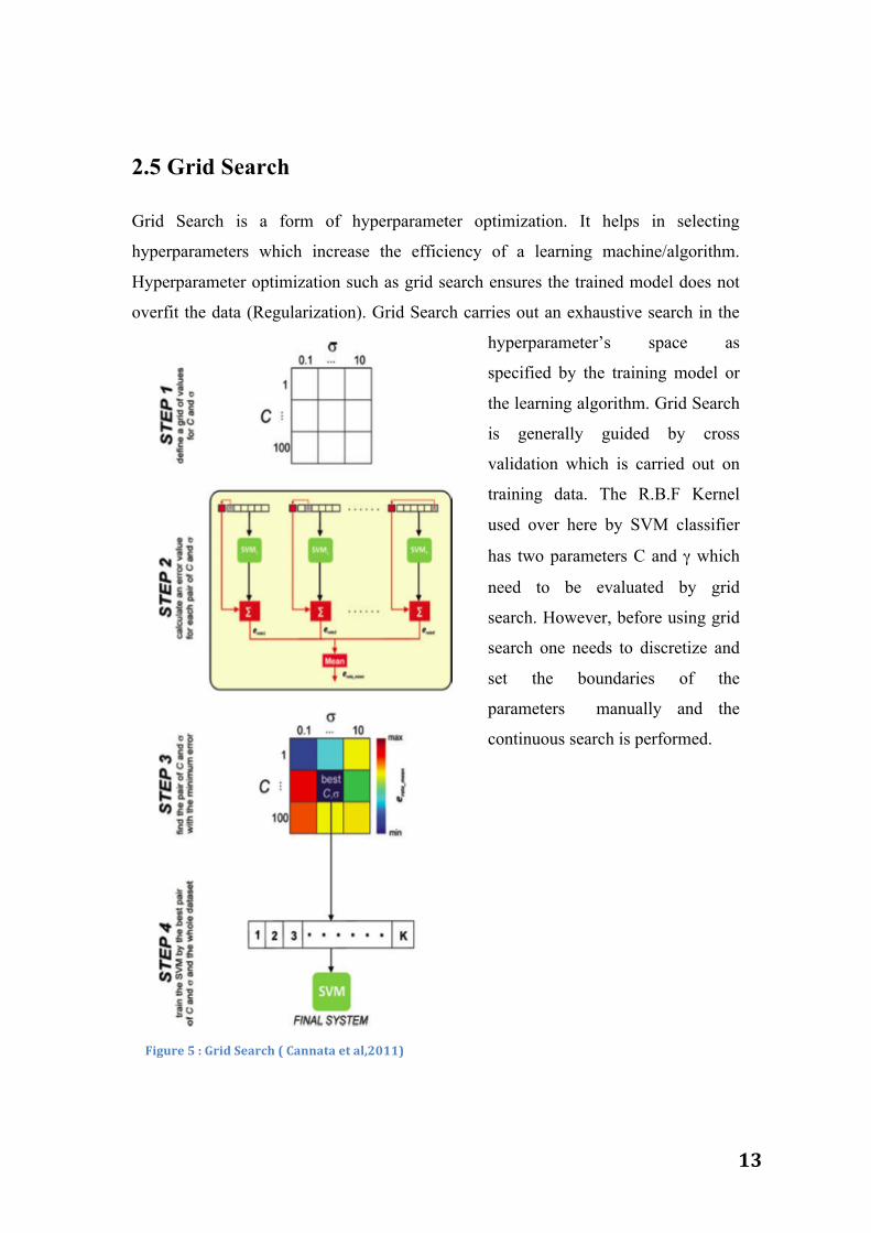
2.5 Grid Search

Grid Search is a form of hyperparameter optimization. It helps in selecting

hyperparameters which increase the efficiency of a learning machine/algorithm.

Hyperparameter optimization such as grid search ensures the trained model does not

overfit the data (Regularization). Grid Search carries out an exhaustive search in the

hyperparameter’s space as

specified by the training model or

the learning algorithm. Grid Search

is generally guided by cross

validation which is carried out on

training data. The R.B.F Kernel

used over here by SVM classifier

has two parameters C and γ which

need to be evaluated by grid

search. However, before using grid

search one needs to discretize and

set the boundaries of the

parameters manually and the

continuous search is performed.

Figure 5 : Grid Search ( Cannata et al,2011)

14

3. Applications And Results.

3.1 Seismic Data

PCAB data has been installed by INGV Naples , Italy in the northern region of

Panarea island which is a Guralp , CMG 40T-60s broadband seismometer (Figure 1) .

The station has been the source of seismic data used for training by SVM

classification technique . On 5th December 2002 , the pump was observed to be

switched on from 06:55 to 10:02 (Universal Time Co-ordinate , UTC) which has been

used for the purpose of training (Figure 2) . Now , for testing the same time series (for

the entire day) has been used which was used for training . Another time series of

seismic signals recorded at PCAB station on 7th December 2002 which had pump

signals switched on at unknown intervals has been tested by the previously mentioned

trained machine . The volcano seismic signal used by Nicola Alessandro Pino et al ,

2011 recorded at the same seismic station on 4th April , 2003 where the seismic

precursors were used for tracking deep gas accumulation and slug upraise has also

been tested by the machine.

Figure 6 : Seismogram of 5th December 2002

15

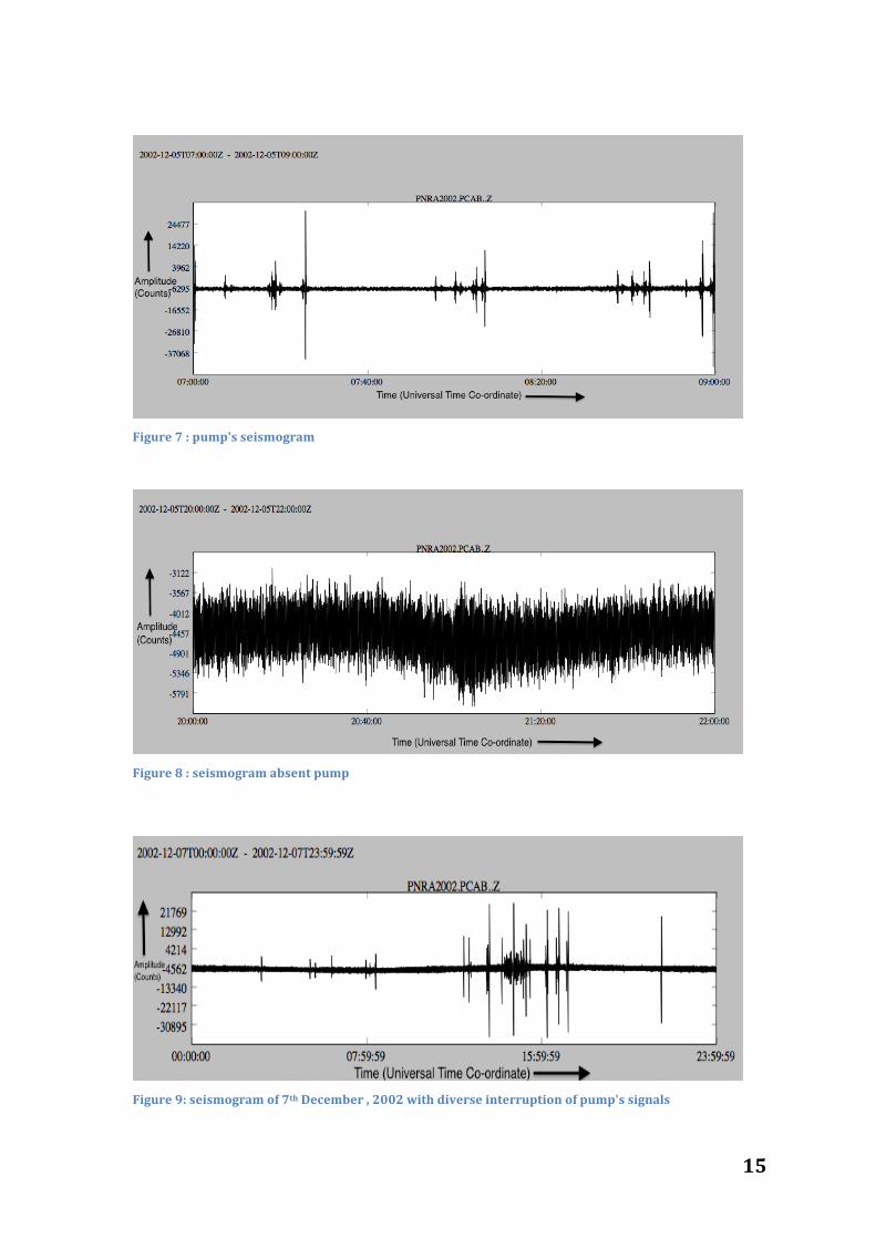
Figure 7 : pump's seismogram

Figure 8 : seismogram absent pump

Figure 9: seismogram of 7th December , 2002 with diverse interruption of pump's signals

16

Figure 10 : Seismogram used by Nicola Alessandro Pino et al, 2011

3.2 Training For training the SVM, Power Spectral Density feature vectors of seismogram

recorded on 5th December 2002 from 07:00 to 09:00 (UTC) (Figure 7) containing

pump signals and 12:00 to 14:00 (UTC) (Figure 8) which do not contain pump signals

have been used. The pump signal containing seismogram ( 07:00 to 09:00 ,UTC) has

been labeled as +1 and the other (12:00 to 14:00 , UTC) has been labeled as -1 when

the pump was observed to be switched on and off respectively .The Kernel function

used here is Radial Basis Function whose C and γ parameters have been calculated by

grid search (an optimizer technique). C = 2048.0 and γ = 0.0001220703125 optimizes

the machine giving 99.7149% correct classification of the parent class determined

through cross validation. SVM1 is the trained model for testing data with a sampling

frequency of 62.5 Hz, which is the sampling frequency of the data used for training

set. SVM2 is the trained model for testing data with a sampling frequency, 31.25 Hz

(seismogram used by Pino et al, 2011) , the sampling frequency of training set data is

reduced to 31.25 Hz and then used for training the model. The SVM applied here uses

200 X 929 points of frequency – time dimensional vectors for training . For getting

homogenious feature vectors we normalized (averaged) the rows of 200 X 929

dimensional matrix.

3.2.1 Grid Search A hyperparameter optimization technique i.e. Grid Search was carried out to

determine the most efficacious C and γ parameters .

17

Figure 11: Grid search for SVM1

Figure 12 : Grid Search for SVM2

18

3.2.2 Cross Validation

Cross Validation of SVM1 and SVM2 has been carried out along with grid search.

The cross validation performed over here is a k fold cross validation with k = 5.

SVM1 : Table 1 : Grid Search and Cross Validation for SVM1

C (Regularization

parameter)

γ (Kernel Parameter)

Accuracy

(5 fold Cross Validation)

32.0 0.078125 99.6579%

2048.0 0.0001220703125 99.7149%

SVM2 : Table 2: Grid Search and Cross Validation for SVM2

C (Regularization

parameter)

γ (Kernel Parameter)

Accuracy

(5 fold Cross Validation)

32.0 0.078125 95.5479%

2048 0.0001220703125 95.6621%

0.5 0.125 96.4612%

19

SVM1 Training

Seismogram containing pump signals For the entire day 5-‐12-‐2002

Slicing

Pump Seismic Signals Pump absent seismic signals

Power Spectral Density

Class : PUMP Label : +1

Class : NO PUMP Label : -‐1

Cross Validation & Grid search

SVM1

20

SVM2

Seismogram containing pump signals

for the entire day 5-‐12-‐2002

Slicing

Pump’s Seismic Signals Pump absent seismic signals

Reduction from 62.5 Hz to 31.25 Hz

Pump’s Seismic Signals Pump absent seismic signals

Class :Pump Label : +1

Class :No Pump Label : -‐1

Cross Validation & Grid Search

SVM2

21

3.4 Testing

SVM1 and SVM2 can be used on spectrograms of seismograms for testing the

presence of pump’s seismic signals. SVM1 machine is used on seismograms with

sampling frequency of 62.5 Hz and SVM2 machine is used on seismograms with

sampling frequency, 31.25 Hz.

Seismogram

Spectrogram

Power Spectral Density

Support Vector Machine

Results

Supervised Classification

22

3.4.1 Testing of original data

Testing the seismogram for the entire day recorded on 5th December, 2002 by SVM1

gives a result that 92.557% of the signals do not contain pump’s seismic signals.

Figure 13 : Spectrogram of the seismogram for the entire day (5-‐12-‐2002) and the corresponding presence of pump signals estimated by black predicted labels

The black predicted labels indicate the presence of pump’s seismic signals estimated

by SVM1 at the corresponding time interval as shown in Figure 13. Incidentally, the

predicted labels coincide with the original pump’s duration of activity, thereby

validating the SVM model and the application of this machine on such problems to

some extent.

23

3.4.2 Testing of data with diverse interruption

The seismogram (sampling rate = 62.5 Hz) for the entire day was recorded on 7th

December, 2002 and it was tested by SVM1 .

Figure 14 : Seismogram of 7-‐12-‐2002 with diverse interruption by pump signals

The machine showed that 97.3637% of the signals do not contain pump’s seismic

signals. It was known that the pump had been active during the day but the exact time

interval of it’s activity was not known which has been estimated by the Support

Vector Machine by the black predicted labels.

Figure 15 : Spectrogram of 7-‐12-‐2002 with corresponding predicted labels estimated by SVM1

24

3.4.3 Testing of data used in Nicola Alessandro Pino et al, 2011.

The seismogram (sampling frequency = 31.25 Hz) recorded by PCAB station on 4th

April , 2003 has been used in Nicola Alessandro Pino et al , 2011 to prove the

existence of deep accumulation of gas and slug upraise in the Stromboli area from a

paroxysmal explosion’s seismic precursors which was basaltic in nature. When the

data was tested by SVM2, the machine showed complete absence of pump’s seismic

signals thereby ,asserting and further authenticating their work.

Figure 16: Seismogram used by Nicola Alessandro Pino et al, 2011

Figure 17: Spectrogram of 04-‐04-‐2003

25

Figure 18: 3-‐dimensional spectrogram of 04-‐04-‐2003

26

5. Discussion

The deterministic approach taken by us by using Support Vector Machines has

overall shown positive results. Apart results from the machine showing

99.7149% accuracy (determined through cross validation) on the parent class,

which was used to train the model, the machine when tested the entire time

series data of the spectrogram obtained from the seismogram of the entire day, it

showed that 92.557% of the seismic signals didn’t contain the pump’s seismic

signals as well as it’s prediction of the pump’s seismic signals presence (which

can be seen in figure 13 marked by black labels) coincides with the observed

duration of activity of the pump. This shows that the machine trained by us is

authentic and is ready for further testing. On 7th December, 2002 it was again

reported the pump was switched on but the duration of activity was unknown.

On using SVM by testing the spectrogram (Power spectral density) of the

seismogram for the entire data we found that 7th December, 2002’s seismic

signals had 97.3637% absent pump’s seismic signals. Although, the black

predicted labels in figure 15 (giving signs of pumps) are spread throughout the

day indicating occurrence of diverse interruption by pump’s seismic signals

which had also been reported by Nicola Aleesandro Pino before the research

work started.

The seismogram of 4th April, 2003 recorded by the same PCAB station (whose

recordings have been used by us for training and testing) had been used by

Nicola Alessandro Pino et al in 2011 where the seismic precursors had been used

by them for suggesting the presence of slug uprise and accumulation of gas deep

in the Earth. The authors were of the view that pump’s seismic signals might have

corrupted the seismogram, hence, rendering the research work done by them

doubtful. The seismogram recorded on that day had a 31.25 Hz as its sampling

frequency which is exactly half of 62.5 Hz, the sampling frequency of the

seismogram used for training the Support Vector Machine. For testing 4th April’s

27

seismogram a new machine was trained (SVM2) by reducing the samples of the

seismogram matrix by half. The algorithm used was :

Si = (s2i+1 + s2i+2)/2 Where i ∈ {0,1,2,3,4,………N}

Here N being the number of samples in the seismogram’s matrix for pump’s seismogram and no pump’s seismogram, reduced separately and then used for training after calculating power spectral density. SVM2 showed an accuracy of 96.4612 % during cross-‐validation. SVM2 tested the 4th April’s spectrogram (power spectral density) and found that the signals didn’t contain the pump’s seismic signals at all thereby subverting the ambiguity and clarifying Nicola Alessandro Pino et al’s work.

28

6. Conclusions The result shows 99.7149% accuracy through cross validation after optimizing using

grid search which is quite high for a supervised classification technique. SVM can

have it’s utility in online data processing too. On the other hand past data records can

also be tested using SVM. SVM can become a useful tool in classification between

signals, which contain noise and signals which do not contain noise in various fields

of Geosciences which involve signal processing. One can supervise the learning

machine by doing a priori labeling of patterns containing noise and then train the

machine using noise containing and noise-free signals. Overall, the performance of

SVM has been interestingly Sui Generis.

1

References Pino, N. A., R. Moretti, P. Allard, and E. Boschi (2011), Seismic precursors of a

basaltic paroxysmal explosion track deep gas accumulation and slug upraise, J.

Geophys. Res., 116, B02312, doi:10.1029/2009JB000826.

Cannata A., Montalto P., Aliotta M., Cassisi, Pulvirenti A., Priviter E. and Patane D.,

Clustering and classification of infrasonic events at Mount Etna using pattern

recognition techniques, Geophys. J. Int. (2011) 185, 253–264

Langer H., Falsaperla S., Masotti M., Campanini R., Spampinato S. and Messina A.,

Synopsis of supervised and unsupervised pattern classification techniques applied to

volcanic tremor data at Mt Etna, Italy, Geophys. J. Int. (2009) 178, 1132–1144

Masotti M., Falsaperla S., Langer H., Spampinato S., and Campanini R., Application

of Support Vector Machine to the classification of volcanic tremor at Etna, Italy,

GEOPHYSICAL RESEARCH LETTERS, VOL. 33, L20304

MathWorks, Inc., “Matlab Products,” [Online document], cited 2013, June 8,

Available HTTP: http://www.mathworks.com/index.html

“LIBSVM – A Library for Support Vector Machines.” LIBSVM – A Library for

Support Vector Machines. N.p., n.d Web. 10 June 2013 [Online Document],

Available Http: www.csie.ntu.edu.tw/~cjlin/libsvm/

2

Appendix

Commands used in command shell of Obspy for extracting seismogram matrix

(matlab format) from raw data :

In [1]: from obspy.core import read

In [2]: from scipy.io import savemat

In [3]: from obspy.core import UTCDateTime

In [4]: from obspy.core import UTCDateTime

In [5]: st =

read("/Users/apple/Desktop/PANAREA/Panarea021205/pcab.021205.z")

In [6]: dt = UTCDateTime("20021205T0655")

In [7]: st =

read("/Users/apple/Desktop/PANAREA/Panarea021205/pcab.021205.z",

starttime = dt , endtime = dt+2*60*60+7*60)

In [8]: for i, tr in enumerate(st):

mdict = dict([[j, str(k)] for j, k in tr.stats.iteritems()])

mdict['data'] = tr.data

savemat("data-‐%d.mat" % i, mdict)

The above commands generate a seismogram matrix of matlab format which can

be read in matlab where it can be plotted and further analyzed by usage of

various mathematical functions.

3

So, we generate two seismogram matrices using UTCDateTime method/function

for slicing the raw data from 06:55 to 09:02 (as we know that the pump signals

are present in the raw data during this time interval) and from 12:00 to 14:07 .

One is having pump signals (pumpo.mat) and the other is not having pump

signals (nopumpo.mat) .

In Matlab :

For normalization :

D = xdata;

[m,n] = size(D);

Su = sum(D);

for i = 1:m , for j = 1:n , N(i,j) = (D(i,j)/Su(1,j));

end

end

N = N';

For generating training data :

>>load pump;

x = double(data);

[S,F,T,P] = spectrogram(x,1024,512,1024,62.5);

v = P(3:202,:)';

load nopump;

x = double(data);


nv = P(3:202,:)';

xdata = vertcat(v,nv);

4

D = xdata;

[m,n] = size(D);

Su = sum(D);

for i = 1:m , for j = 1:n , N(i,j) = (D(i,j)/Su(1,j));

end

end

N = N';

tdata = sparse(N);

for j=1:929, c(j)=1;

end

c = c';

for j=1:929, nc(j)=-‐1;

end

nc = nc';

group = vertcat(c,nc);

save('train','tdata','group');

The above program generates a file which can be used in svm program for

carrying out training .

For generating testing data in matlab :

load data;

x = double(data);


5

test = P(3:202,:)';

D = xdata;

[m,n] = size(D);

Su = sum(D);

for i = 1:m , for j = 1:n , N1(i,j) = (D(i,j)/Su(1,j));

end

end

N1 = N1';

test = sparse(N1);

for j=1:10545 , group1(j) = -‐1;

end

group1 = group1';

save('test','test','group1');

The above program generates a file which can be used in svm program for

carrying out testing. Here data.m is the seismogram matrix which has to be

classified by svm classifier generated by ObsPy.

The svm program used is a unix based program from libsvm-‐3.16 package which

can be downloaded from :

http://www.csie.ntu.edu.tw/~cjlin/libsvm/

6

and for running the “makefile” one needs a gcc compiler for linux platforms , x

code for macintosh platforms , for windows the program is already available in

the package and other c++ , matlab , python plug-‐ins are also available within the

package. After running the Makefile , “svm-‐train” , “svm-‐predict” , “svm-‐scale” are

automatically created .

Training :

In unix shell :

macbook-‐air-‐13:~ apple$ cd Desktop/libsvm-‐3.16/

macbook-‐air-‐13:libsvm-‐3.16 apple$ ./svm-‐scale -‐l -‐1 -‐u 1 -‐s range1

"/Users/apple/Desktop/train.txt" > train.scale

macbook-‐air-‐13:libsvm-‐3.16 apple$ ./svm-‐train train.scale

*

optimization finished, #iter = 350

7

nu = 0.569305

obj = -‐412.293341, rho = 0.134911

nSV = 547, nBSV = 515

Total nSV = 547

First the data is scaled and then it is trained , after this process a

“train.scale.model” file is created which can be used for testing purposes

Testing :

macbook-‐air-‐13:libsvm-‐3.16 apple$./svm-‐scale -‐r range1

"/Users/apple/Desktop/test.txt" > test.scale

macbook-‐air-‐13:libsvm-‐3.16 apple$ ./svm-‐predict test.scale train.scale.model

test.predict

Accuracy = 90.625% (841/928) (classification)

macbook-‐air-‐13:libsvm-‐3.16 apple$

One can generate predicted labels by adding :

printf("%g\n",predict_label);

in 138th line of svm-‐predict.c file of libsvm-‐3.16 , obtained from libsvm package

and then compiling it again to generate the svm-‐predict program.

For generating seismogram and then integrating it with predicted labels

pictorially. (in Matlab) :

for i = 1:10545 , yn(1,i) = 0.5;

end

for i = 1:10545 , if numneric(i,1)>0 numneric(i,1)= 90;

else numneric(i,1) = 30;

end

end;

8

zn = numneric';

x = double(data);

figure;

h(1) = subplot(2,1,1);

[y,f,t,p] = spectrogram(x,1024,512,1024,31.25,'yaxis');

surf(t,f,10*log10(abs(p)),'EdgeColor','none');

axis xy; axis tight; colormap(jet); view(0,90);

h(2) = subplot(2,1,2);

dotsize = 25;

scatter(t(:),yn(:), dotsize, zn(:));

linkaxes(h,'x');

Documents

Application Of Support Vector Machines For Seismogram