Embed Size (px)
Citation preview

8/9/2019 Application of Sensitivity Analysis
http://slidepdf.com/reader/full/application-of-sensitivity-analysis 1/42
APPLICATION OF SENSITIVITY ANALYSIS IN CAPITAL BUDGETING
A.I.M.S. 1
1.INTRODUCTION

8/9/2019 Application of Sensitivity Analysis
http://slidepdf.com/reader/full/application-of-sensitivity-analysis 2/42
APPLICATION OF SENSITIVITY ANALYSIS IN CAPITAL BUDGETING
A.I.M.S. 2
RISK ANALYSIS
Risk is inherent in almost every business decision. More so in capital budgeting decisions as
they involve costs and benefits extending over a long period of time during which many
things can change in unanticipated ways.
For the sake of expository convenience, we assume that all investments considered for inclusion in the capital budget have the same risk as those of the existing investments of the
firm. Hence, average cost of Capital is used for evaluating the project. But, investment
proposals differ in risk. A research and development project may be more risky than an
expansion project and the latter tends to be more risky than a replacement project. In view of
such differences, variations in risk need to be considered explicitly in capital investment
appraisal.
Risk analysis is one of the mist complex and slippery aspects of capital budgeting. Many
different techniques have been suggested and no single technique can be deemed as best in all
situations. The variety of techniques suggested for handling risk in capital budgeting fall into
two broad categories:
i. Approaches that consider the standalone risk of a project.
ii. Approaches that consider the risk of a project in the context of the firm or in the
context of the market.
Risk analysis is a technique to identify and assess for mitigation of risks, at project initiation
and during task execution. It therefore attempts to identify any factors that can place a project
in jeopardy before and during the execution of the work, assigning ownership of each risk.
The advantage of this approach is that it is clear to all sides, vendor, contractors and
purchaser, what the risks are and who has ownership of each one. Also, it identifies risks
introduced into the project by all parties, whether they have a sustainable relationship with
the organization performing the work.
This approach to mitigating the risk factors also helps to define preventive measures to
reduce the probability of occurrence and identify methods to avert possible negative effects
on the effectiveness of the company to compete in this particular market.

8/9/2019 Application of Sensitivity Analysis
http://slidepdf.com/reader/full/application-of-sensitivity-analysis 3/42
APPLICATION OF SENSITIVITY ANALYSIS IN CAPITAL BUDGETING
A.I.M.S. 3
SOURCES OF RISK
There are several sources of risk in a project. Some of the risks are:
Project-specific risk
The earnings and cash flows of the project may be lower than expected because of estimationerror or some factors specific to the project like the quality of management.
Competitive risk
The earnings and cash flows of the project may be affected by unanticipated actions of
competitors.
Industry-specific risk
Unexpected technological developments and regulatory changes, that are specific to the
industry to which the project belongs will have an impact on the earnings and cash flows of
the project as well.
Market risk
Unanticipated changes in macroeconomic factors like the GDP growth rate, interst rate, and
inflation have an impact on all projects, albeit in varying degrees.
International risk
In the case of a foreign project, the earnings and cash flows may be different than expected
due to exchange rate risk or political risk.

8/9/2019 Application of Sensitivity Analysis
http://slidepdf.com/reader/full/application-of-sensitivity-analysis 4/42
APPLICATION OF SENSITIVITY ANALYSIS IN CAPITAL BUDGETING
A.I.M.S. 4
PERSPECTIVES ON RISK
Regardless of the risk measure employed, there are different perspectives on risk. The project
can be viewed from at least three different perspectives. These are:
Stand-alone risk
This represents the risk of a project when it is viewed in isolation.
Firm Risk
It is also called corporate risk. This represents the contribution of the project to risk of the
firm.
Market Risk
This represents the risk of a project from the point of view of a diversified investor. It is also
called systematic risk.
Since the primary goal of the firm is to maximise shareholder value, what matters finally is
the risk that a project imposes on shareholders. If shareholders are well diversified, market
risk is the most appropriate measure of risk.
In practice, however, the project¶s standalone risks as well as its corporate risks are
considered important.
The project¶s standalone risk is considered important for the following reasons.
y Measuring a project¶s stand-alone risk is easier than measuring its corporate risk and
far easier than measuring its market risk.
y In most of the cases, standalone risk, corporate risk, and market risk are highly
correlated. If the overall economy does well, the firm too would do well. Further, if
the firm does well, most of its projects would do well. Thanks to this high correlation,
standalone risk may be used as a proxy for corporate risk and market risk.
y The proponent of a capital investment is likely to be judged on the performance of
that investment. Hence he will naturally be concerned baout its stand-alone risk and
not about its contribution to the risk of the firm or the risk of a diversified investor.
y In most firms, the capital budgeting committee considers investment proposals one at
a time. The committee often does not have the time or information or expertise to
fully consider the interactions of the investments with the other investments of the
firm or its shareholders.
Corporate risk is considered important for the following reasons:
y Undiversified shareholders are more concerned about corporate risk than market risk.
Promoters who generally have a substantial equity stake tend to be undiversified or
poorly diversified shareholders.
8/9/2019 Application of Sensitivity Analysis
http://slidepdf.com/reader/full/application-of-sensitivity-analysis 5/42
APPLICATION OF SENSITIVITY ANALYSIS IN CAPITAL BUDGETING
A.I.M.S. 5
y Empirical studies suggest that both market risk and corporate risk have a bearing on
required returns. Perhaps even diversified investors consider corporate risk in addition
to market risk when they specify required returns.
y The stability of overall corporate cash flows and earnings is valued by managers,
workers, suppliers, creditors, customers and the community in which the firm
operates. If the cash flow and earnings of the firm are perceived to be highly volatileand risky, the firm will have difficulty in attracting talented employees, loyal
customers, reliable suppliers, and dependable lenders. This will impair its
performance and destroy shareholder wealth.

8/9/2019 Application of Sensitivity Analysis
http://slidepdf.com/reader/full/application-of-sensitivity-analysis 6/42
APPLICATION OF SENSITIVITY ANALYSIS IN CAPITAL BUDGETING
A.I.M.S. 6
2.FINANCIAL ANALYSIS
TECHNIQUES

8/9/2019 Application of Sensitivity Analysis
http://slidepdf.com/reader/full/application-of-sensitivity-analysis 7/42
APPLICATION OF SENSITIVITY ANALYSIS IN CAPITAL BUDGETING
A.I.M.S. 7
FINANCIAL ANALYSIS TECHNIQUES
1. Simple Pay Back Period:
Simple Payback Period (SPP) represents, as a first approximation; the time (number of years)
required to recover the initial investment (First Cost), considering only the Net Annual
Saving:
The simple payback period is usually calculated as follows:
Simple payback Period = {First Cost / (Yearly Benefits ± Yearly Costs)}
Examples
Simple payback period for a continuous Deodorizer that costs Rs.60 lakhs to purchase and
install, Rs.1.5 lakhs per year on an average to operate and maintain and is expected to save
Rs. 20 lakhs by reducing steam consumption (as compared to batch deodorizers), may be
calculated as follows:
Simple Payback Period = {60 / (20 - 1.5)}
= 3 years 3 months
According to the payback criterion, the shorter the payback period, the more desirable is the
project.
Advantages
A widely used investment criterion, the payback period seems to offer the following
advantages:
y It is simple, both in concept and application. Obviously a shorter payback generallyindicates a more attractive investment. It does not use tedious calculations.
y It favours projects, which generate substantial cash inflows in earlier years, and
discriminates against projects, which bring substantial cash inflows in later years but
not in earlier years.
Limitations
y It fails to consider the time value of money. Cash inflows, in the payback
calculation, are simply added without suitable discounting. This violates the most
basic principle of financial analysis, which stipulates that cash flows occurring atdifferent points of time can be added or subtracted only after suitable
compounding/discounting.
y It ignores cash flows beyond the payback period. This leads to discrimination
against projects that generate substantial cash inflows in later years.

8/9/2019 Application of Sensitivity Analysis
http://slidepdf.com/reader/full/application-of-sensitivity-analysis 8/42
APPLICATION OF SENSITIVITY ANALYSIS IN CAPITAL BUDGETING
A.I.M.S. 8
To illustrate, consider the cash flows of two projects, A and B:
Investment Rs. (100,000) Rs.(100,000)
Savings in Year Cash Flow of A Cash flow of B
1 50,000 20,000
2 30,000 20,0003 20,000 20,000
4 10,000 40,000
5 10,000 50,000
6 - 60,000
The payback criterion prefers A, which has a payback period of 3 years, in comparison to B,
which has a payback period of 4 years, even though B has very substantial cash inflows in
years 5 and 6.
y It is a measure of a project¶s capital recovery, not profitability.
y Despite its limitations, the simple payback period has advantages in that it may be
useful for evaluating an investment.
Time Value of Money
A project usually entails an investment for the initial cost of installation, called the capital
cost, and a series of annual costs and/or cost savings (i.e. operating, energy, maintenance,
etc.) throughout the life of the project. To assess project feasibility, all these present and
future cash flows must be equated to a common basis. The problem with equating cash flows
which occur at different times is that the value of money changes with time. The method by
which these various cash flows are related is called discounting, or the present value
concept.
For example, if money can be deposited in the bank at 10% interest, then a Rs.100 deposit
will be worth Rs.110 in one year's time. Thus the Rs.110 in one year is a future value
equivalent to the Rs.100 present value.
In the same manner, Rs.100 received one year from now is only worth Rs.90.91 in today's
money (i.e. Rs.90.91 plus 10% interest equals Rs.100). Thus Rs.90.91 represents the present
value of Rs.100 cash flow occurring one year in the future. If the interest rate were something
different than 10%, then the equivalent present value would also change. The relationship between present and future value is determined as follows:
Future Value (FV) = NPV (1 + i)n
or NPV = FV / (1+i)n
Where
FV = Future value of the cash flow

8/9/2019 Application of Sensitivity Analysis
http://slidepdf.com/reader/full/application-of-sensitivity-analysis 9/42
APPLICATION OF SENSITIVITY ANALYSIS IN CAPITAL BUDGETING
A.I.M.S. 9
NP V= N et P resent Value of the cash flow
i = Interest or discount rate
n = N umber of years in the future
2. Return on Investment (ROI)ROI expresses the "annual return" from the project as a percentage of capital cost. The annual
return takes into account the cash flows over the project life and the discount rate by
converting the total present value of ongoing cash flows to an equivalent annual amount over
the life of the project, which can then be compared to the capital cost. ROI does not require
similar project life or capital cost for comparison.
This is a broad indicator of the annual return expected from initial capital investment,
expressed as a percentage:
ROI = { (Annual Net Cash Flow / Capital Cost) x 100 }
ROI must always be higher than cost of money (interest rate); the greater the return on
investment better is the investment.
Limitations
y It does not take into account the time value of money.
y It does not account for the variable nature of annual net cash inflows.
3. Net Present Value
The net present value (NPV) of a project is equal to the sum of the present values of all the
cash flows associated with it. Symbolically,
Where NPV = Net Present Value
CFt= Cash flow occurring at the end of year µt¶ (t=0,1,«.n)
n = life of the project
= Discount rate
The discount rate () employed for evaluating the present value of the expected future cash
flows should reflect the risk of the project.
NPV = {(CF0
/ (1 + )0
) + ( CF1
/ (1 + )1
) + - - - + ( CFn
/ (1 + )n
)
Example
To illustrate the calculation of net present value, consider a project, which has the following
cash flow stream:

8/9/2019 Application of Sensitivity Analysis
http://slidepdf.com/reader/full/application-of-sensitivity-analysis 10/42
APPLICATION OF SENSITIVITY ANALYSIS IN CAPITAL BUDGETING
A.I.M.S. 10
Investment Rs. (1,000,000)
Saving in Year Cash flow
1 200,000
2 200,000
3 300,000
4 300,000
5 350,000
The cost of capital, , for the firm is 10 per cent. The net present value of the proposal is:
NPV = {(1,000,000/(1.10)0
) + (200,000/(1.10)1
) + (200,000/(1.10)2
) + (300,000/(1.10)3
) +
(300,000/(1.10)4
) + (350,000/(1.10)5
)}
= (5,273)
The net present value represents the net benefit over and above the compensation for time and
risk.
Hence the decision rule associated with the net present value criterion is: ³Accept the project if
the net present value is positive and reject the project if the net present value is negative´.
Advantages
The net present value criterion has considerable merits.
y It takes into account the time value of money.
y It considers the cash flow stream in its project life.
4. Internal Rate of Return
This method calculates the rate of return that the investment is expected to yield. The internal rate
of return (IRR) method expresses each investment alternative in terms of a rate of return (a
compound interest rate). The expected rate of return is the interest rate for which total discounted
benefits become just equal to total discounted costs (i.e net present benefits or net annual benefits
are equal to zero, or for which the benefit / cost ratio equals one). The criterion for selection
among alternatives is to choose the investment with the highest rate of return.

8/9/2019 Application of Sensitivity Analysis
http://slidepdf.com/reader/full/application-of-sensitivity-analysis 11/42
APPLICATION OF SENSITIVITY ANALYSIS IN CAPITAL BUDGETING
A.I.M.S. 11
The rate of return is usually calculated by a process of trial and error, whereby the net cash
flow is computed for various discount rates until its value is reduced to zero.
The internal rate of return (IRR) of a project is the discount rate, which makes its net present
value (NPV) equal to zero. It is the discount rate in the equation:
NPV = {(CF0
/ (1 + )0
) + ( CF1
/ (1 + )1
) + - - - + ( CFn
/ (1 + )n
) = 0
Where, CFn= Cash flow at the end of year ³n´
= discount rate
n = life of the project.
CFtvalue will be negative if it is expenditure and positive if it is savings.
In the net present value calculation we assume that the discount rate (cost of capital) is known
and determine the net present value of the project. In the internal rate of return calculation,
we set the net present value equal to zero and determine the discount rate (internal rate of return), which satisfies this condition.
To illustrate the calculation of internal rate of return, consider the cash flows of a project:
Year 0 1 2 3 4
Cash Flow (100,000) 30,000 30,000 40,000 45,000
The internal rate of return is the value of ³ k ´ which satisfies the following equation:
The calculation of ³´ involves a process of trial and error. We try different values of ³´ till
we find that the right-hand side of the above equation is equal to 100,000. Let us, to begin
with, try = 15 per cent. This makes the right-hand side equal to:
{(30000/1.15) + (30000/(1.15)2
) + (40000/(1.15)3
) + (45000/(1.15)4
) + ----- + -----}
= 100, 802
This value is slightly higher than our target value, 100,000. So we increase the value of
from 15 per cent to 16 per cent. (In general, a higher lowers and a smaller r increases the
right-hand side value). The right-hand side becomes:
{(30000/1.16) + (30000/(1.16)
2
) + (40000/(1.16)
3
) + (45000/(1.16)
4
) + ----- + -----
= 98,641
Since this value is now less than 100,000, we conclude that the value of k lies between 15 per
cent and 16 per cent. For most of the purposes this indication suffices.

8/9/2019 Application of Sensitivity Analysis
http://slidepdf.com/reader/full/application-of-sensitivity-analysis 12/42
APPLICATION OF SENSITIVITY ANALYSIS IN CAPITAL BUDGETING
A.I.M.S. 12
Advantages
A popular discounted cash flow method, the internal rate of return criterion has several
advantages:
y It takes into account the time value of money.
y It considers the cash flow stream in its entirety.
y It makes sense to businessmen who prefer to think in terms of rate of return and find
an absolute quantity, like net present value, somewhat difficult to work with.
Limitations
y The internal rate of return figure cannot distinguish between lending and borrowing
and hence a high internal rate of return need not necessarily be a desirable feature.
Example
Calculate the internal rate of return for an economizer that will cost Rs. 500,000 will last 10
years, and will result in fuel savings of Rs. 150,000 each year.
Find the i that will equate the following:
Rs. 500,000 = 150,000 x PV (A = 10 years, i = ?)
To do this, calculate the net present value (NPV) for various i values, selected by visual
inspection;
NPV 25% = Rs. 150,000 x 3.571 ± Rs. 500,000
Rs. 35,650
NPV 30% = Rs. 150,000 x 3.092 ± Rs. 500,000
= -Rs. 36,200
For,
i = 25 per cent, net present value is positive;
i = 30 per cent, net present value is negative.
Thus, for some discount rate between 25 and 30 per cent, present value benefits are equated
to present value costs. To find the rate more exactly, one can interpolate between the tworates as follows:
i = 0.25 + (0.30-0.25) x 35650 / (35650 + 36200)
= 0.275 or 27.5 percent

8/9/2019 Application of Sensitivity Analysis
http://slidepdf.com/reader/full/application-of-sensitivity-analysis 13/42
APPLICATION OF SENSITIVITY ANALYSIS IN CAPITAL BUDGETING
A.I.M.S. 13
Cash Flows
Generally there are two kinds of cash flow; the initial investment as one or more instalments,
and the savings arising from the investment. This over simplifies the reality of energy
management investment.
There are usually other cash flows related to a project. These include the following:
y Capital costs are the costs associated with the design, planning, installation and
commissioning of the project; these are usually one-time costs unaffected by inflation
or discount rate factors, although, as in the example, instalments paid over a period of
time will have time costs associated with them.
y Annual cash flows, such as annual savings accruing from a project, occur each year
over the life of the project; these include taxes, insurance, equipment leases, energy
costs, servicing, maintenance, operating labour, and so on. Increases in any of these
costs represent negative cash flows, whereas decreases in the cost represent positive
cash flows.
Factors that need to be considered in calculating annual cash flows are:
y Taxes, using the marginal tax rate applied to positive (i.e. increasing taxes) or
negative (i.e. decreasing taxes) cash flows.
y Asset depreciation, the depreciation of plant assets over their life; depreciation is a
³paper expense allocation´ rather than a real cash flow, and therefore is not included
directly in the life cycle cost. However, depreciation is ³real expense´ in terms of tax
calculations, and therefore does have an impact on the tax calculation noted above.
For example, if a Rs.10,00,000 asset is depreciated at 20% and the marginal tax rate
is 40%, the depreciation would be Rs.200,000 and the tax cash flow would be
Rs.80,000 and it is this later amount that would show up in the costing calculation.
y Intermittent cash flows occur sporadically rather than annually during the life of the
project, relining a boiler once every five years would be an example.

8/9/2019 Application of Sensitivity Analysis
http://slidepdf.com/reader/full/application-of-sensitivity-analysis 14/42
APPLICATION OF SENSITIVITY ANALYSIS IN CAPITAL BUDGETING
A.I.M.S. 14
3.TECHNIQUES
FOR RISK ANALYSIS

8/9/2019 Application of Sensitivity Analysis
http://slidepdf.com/reader/full/application-of-sensitivity-analysis 15/42
APPL AT E T T ANAL N CAPITAL B ETING
A.I.M.S. 15
TECHNIQUES FOR RISK ANAL SIS
Techni esof Risk
Anal sis
Anal sis of Standalone
R sik
Sensiti ityAnalysis
Scenar ioAnalysis
Analysis of Contexual
r isk
Corporate
Risk Analysis
Market Risk
Analysis

8/9/2019 Application of Sensitivity Analysis
http://slidepdf.com/reader/full/application-of-sensitivity-analysis 16/42
APPLICATION OF SENSITIVITY ANALYSIS IN CAPITAL BUDGETING
A.I.M.S. 16
SENSITIVITY AND RISK ANALYSIS
Many of the cash flows in the project are based on assumptions that have an element of
uncertainty. The present day cash flows, such as capital cost, energy cost savings,
maintenance costs, etc. can usually be estimated fairly accurately. Even though these costs
can be predicted with some certainty, it should always be remembered that they are onlyestimates. Cash flows in future years normally contain inflation components which are often
"guess-timates" at best. The project life itself is an estimate that can vary significantly.
Sensitivity analysis is an assessment of risk. Because of the uncertainty in assigning values to
the analysis, it is recommended that a sensitivity analysis be carried out - particularly on
projects where the feasibility is marginal. How sensitive is the project's feasibility to changes
in the input parameters? What if one or more of the factors in the analysis is not as favourable
as predicted? How much would it have to vary before the project becomes unviable? What is
the probability of this happening?
Suppose, for example, that a feasible project is based on an energy cost saving that escalates
at 10% per year, but a sensitivity analysis shows the break-even is at 9% (i.e. the project
becomes unviable if the inflation of energy cost falls below 9%). There is a high degree of
risk associated with this project - much greater than if the break-even value was at 2%.
Many of the computer spreadsheet programs have built-in "what if" functions that make
sensitivity analysis easy. If carried out manually, the sensitivity analysis can become
laborious - reworking the analysis many times with various changes in the parameters.
Sensitivity analysis is undertaken to identify those parameters that are both uncertain and for
which the project decision, taken through the NPV or IRR, is sensitive. Switching values
showing the change in a variable required for the project decision to change from acceptance
to rejection are presented for key variables and can be compared with post evaluation results
for similar projects. For large projects and those close to the cut-off rate, a quantitative risk analysis incorporating different ranges for key variables and the likelihood of their occurring
simultaneously is recommended. Sensitivity and risk analysis should lead to improved project
design, with actions mitigating against major sources of uncertainty being outlined
The various micro and macro factors that are considered for the sensitivity analysis are listed
below.
Micro factors
y Operating expenses (various expenses items)
y Capital structurey Costs of debt, equity
y Changing of the forms of finance e.g. leasing
y Changing the project duration
8/9/2019 Application of Sensitivity Analysis
http://slidepdf.com/reader/full/application-of-sensitivity-analysis 17/42
APPLICATION OF SENSITIVITY ANALYSIS IN CAPITAL BUDGETING
A.I.M.S. 17
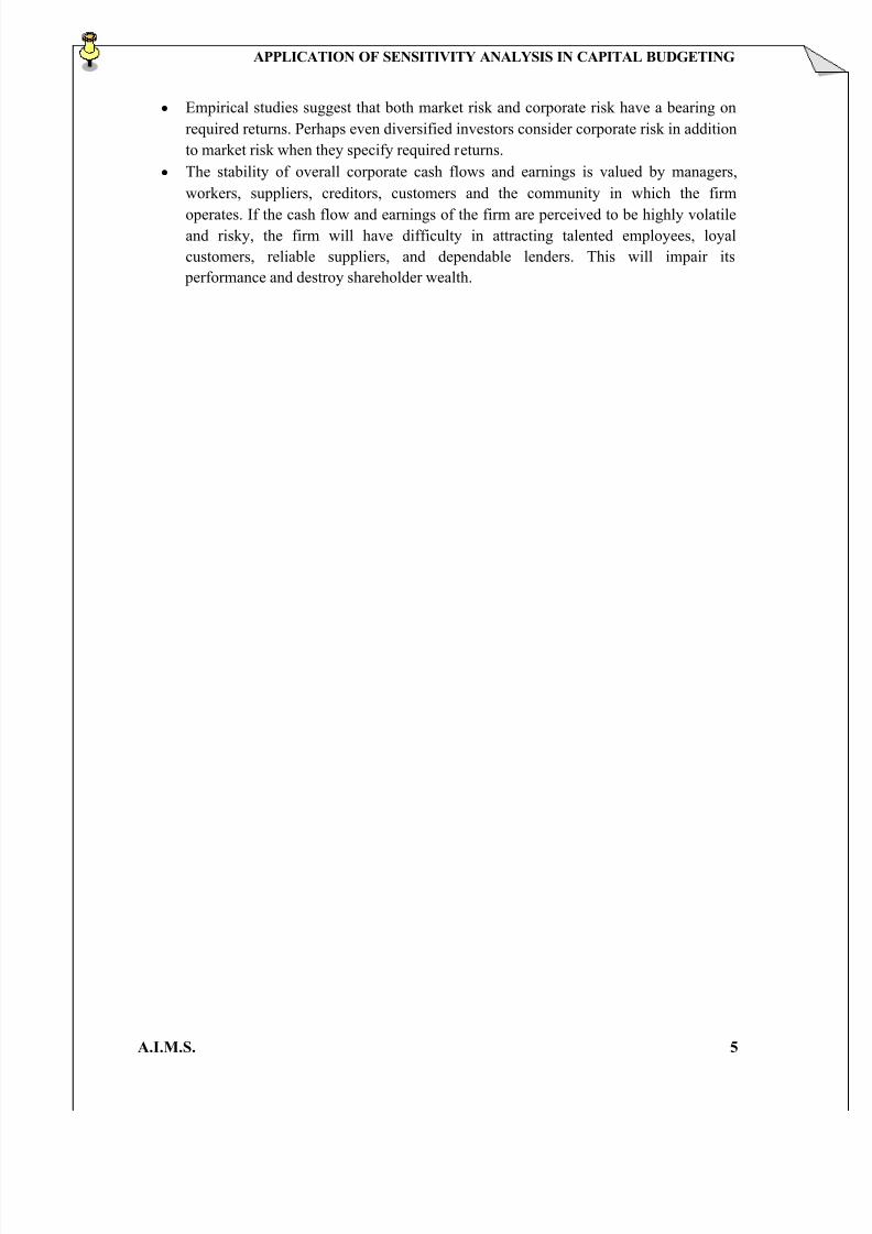
Macro factors
Macro economic variables are the variable that affects the operation of the industry of which
the firm operates. They cannot be changed by the firm¶s management.
Macro economic variables, which affect projects, include among others:y Changes in interest rates
y Changes in the tax rates
y Changes in the accounting standards e.g. methods of calculating depreciation
y Changes in depreciation rates
y Extension of various government subsidized projects e.g. rural electrification
y General employment trends e.g. if the government changes the salary scales
y Imposition of regulations on environmental and safety issues in the industry
y Energy Price change
y Technology changes
The sensitivity analysis will bring changes in various items in the analysis of financial
statements or the projects, which in turn might lead to different conclusions regarding the
implementation of projects.
Evaluation
A very popular method for assessing risk, sensitivity analysis has certain merits:
y It shows how robust or vulnerable a project is to changes in values of the underlying
variables.
y It indicates where further work may be done. If the net present value is highly
sensitive to changes in some factor, it may be worthwhile to explore how the
variability of that critical factor may be contained.
y It is intuitively very appealing as it articulates the concerns that project evaluators
normally have.
Notwithstanding its appeal and popularity, sensitivity analysis suffers from several
shortcomings:
y It merely shows what happens to NPV when there is a change in some variable,
without providing any idea of how likely that change will be.
y Typically, in sensitivity analysis only one variable is changed at a time. In the real
world, however, variables tend to move together.
y It is inherently a very subjective analysis. The same sensitivity analysis may lead one
decision maker to accept the project while another may reject it.

8/9/2019 Application of Sensitivity Analysis
http://slidepdf.com/reader/full/application-of-sensitivity-analysis 18/42
APPLICATION OF SENSITIVITY ANALYSIS IN CAPITAL BUDGETING
A.I.M.S. 18
SCENARIO ANALYSIS
Scenario analysis is a process of analysing possible future events by considering alternative
possible outcomes (scenarios). The analysis is designed to allow improved decision-making
by allowing more complete consideration of outcomes and their implications.
For example, in economics and finance, a financial institution might attempt to forecast
several possible scenarios for the economy (e.g. rapid growth, moderate growth, slow
growth) and it might also attempt to forecast financial market returns (for bonds, stocks and
cash) in each of those scenarios. It might consider sub-sets of each of the possibilities. It
might further seek to assign probabilities to the scenarios (and sub-sets if any). Then it will be
in a position to consider how to distribute assets between asset types (i.e. asset allocation );
the institution can also calculate the scenario-weighted expected return (which figure will
indicate the overall attractiveness of the financial environment).
Depending on the complexity of the financial environment, in economics and finance
scenario analysis can be a demanding exercise. It can be difficult to foresee what the futureholds (e.g. the actual future outcome may be entirely unexpected), i.e. to foresee what the
scenarios are, and to assign probabilities to them; and this is true of the general forecasts
never mind the implied financial market returns. The outcomes can be modelled
mathematically/statistically e.g. taking account of possible variability within single scenarios
as well as possible relationships between scenarios.
Financial institutions can take the analysis further by relating the asset allocation that the
above calculations suggest to the industry or peer group disposition of assets. In so doing the
financial institution seeks to control its business risk rather than the client's portfolio risk.
Procedure
The steps involved in scenario analysis are as follows:
a. Select the factors around which the scenarios will be built. The factor chosen must be
the largest source of uncertainty for the success of the project. It may be the state of
the economy or interest rate or technological development or response of the market.
b. Estimate the values of each of the variables in investment analysis (investment outlay,
revenues, costs, project life, and so on) for each scenario.
c. Calculate the next present value and / or internal rate of return under each scenario.
Best and Worst Case Analysis
Firms often do a kind of scenario analysis called the best case and worst case analysis. In this
kind of analysis the following scenarios are considered:
Best Scenario: High Demand, high selling price, low variable cost, and so on.

8/9/2019 Application of Sensitivity Analysis
http://slidepdf.com/reader/full/application-of-sensitivity-analysis 19/42
APPLICATION OF SENSITIVITY ANALYSIS IN CAPITAL BUDGETING
A.I.M.S. 19
Normal Scenario: Average demand, average selling price, high variable cost, and so on.
Worst Scenario: Low demand, low selling price, high variable cost, and so on.
The objective of such a scenario analysis is to get a feel of what happens under the most
favourable or the most adverse configuration of key variables, without bothering much about
the internal consistency of such configurations.
Evaluation
Scenario Analysis may be considered as an improvement over Sensitivity Analysis because it
considers variations in several variables together.
However, Scenario analysis has its own limitations:
y It is based on the assumption that there are few well- delineated scenarios. This may
not be true in many cases. For example, the economy does not necessarily lie in threediscrete states, viz. recession, stability, and boom. It can in fact be anywhere on the
continuum between the extremes. When a continuum is converted into three discrete
states some information is lost.
y Scenario analysis expands the concept of estimating the expected values. Thus in a
case where there are 10 inputs, the analyst has to estimate 30 expected values (3 x 10)
to do the scenario analysis.

8/9/2019 Application of Sensitivity Analysis
http://slidepdf.com/reader/full/application-of-sensitivity-analysis 20/42
APPLICATION OF SENSITIVITY ANALYSIS IN CAPITAL BUDGETING
A.I.M.S. 20
RISK ANALYSIS IN PRACTICE
Several methods to incorporate the risk factor into capital expenditure analysis are used in
practice. The most common ones are:
Conservative Estimation of Revenues
In many cases the revenues expected from a project are conservatively estimated to ensure
that the viability of the projects is not easily threatened by unfavourable circumstances. The
capital budgeting systems often have built-in devices for conservative estimation. This is
indicated by the following remarks made by two executives:
³We ask the project sponsor to estimate revenues conservatively. This checks the optimism
common among project sponsors.´
³The Capital budgeting committee requires justification for revenue figures given by those
who propose capital expenditures. This has a sobering effect on them.´
Safety Margin in Cost Figures
A margin of safety is generally included in estimating cost figures. This varies between 10
percent and 30 percent of what is deemed as normal cost. The size of the margin depends on
what management feels about the likely variation in cost. The following observation suggests
this:
³In estimating the cost of raw material we add about 20 to 25 percent to the current prices as
the raw material price is not stable and often we pay a high price to get it. For labour cost we
add about 10 to 12 percent as this is the annual increase.´
Flexible Investment Yardsticks
The cut-off point on an investment varies according to the judgement of management about
the riskiness of the project. In one company replacement investments are okayed if the
expected post-tax return exceeds 15 percent but new investments are undertaken only if the
expected post-tax return is greater than 20 percent. Another company employs a short
payback period of three year for new investments. Its decision rule was stated by its financial
controller as follows:
³Our policy is to accept a new project only if it has a payback period of three years. We have
never, as far as I know, deviated from this. The use of short payback period automatically
weeds out risky projects.´

8/9/2019 Application of Sensitivity Analysis
http://slidepdf.com/reader/full/application-of-sensitivity-analysis 21/42
APPLICATION OF SENSITIVITY ANALYSIS IN CAPITAL BUDGETING
A.I.M.S. 21
Sensitivity Analysis
It is a common practice to judge how robust or vulnerable a project is to adverse variations in
the values of the underlying variables like selling price, raw material cost, and quantity sold.
As a manager puts it as:
³We examine the impact of 5 percent and 10 percent adverse variation in selling price, raw
material cost, and quantity sold on NPV and IRR.´
Scenario Analysis
Companies often look at a few scenarios and the top management or the board of directors
decides on the basis of such information. Two examples are given below:
In a pharmaceutical company sponsors are required to give three estimates of rate of return:
most pessimistic, most likely and most optimistic.
In a shipping company three estimates, labelled high, medium, and low are developed for
proposed investments.
Relative Importance of Various Methods of Assessing Project Risk:
% of companies rating it as very
important or important
y Sensitivity Analysis 90.10
y Scenario Analysis 61.60
y Risk-adjusted Discount rate 31.70
y Decision Tree Analysis 12.20
y Monte Carlo Simulation 8.20

8/9/2019 Application of Sensitivity Analysis
http://slidepdf.com/reader/full/application-of-sensitivity-analysis 22/42
APPLICATION OF SENSITIVITY ANALYSIS IN CAPITAL BUDGETING
A.I.M.S. 22
4. APPLICATION OF
SENSITIVITY ANALYSIS

8/9/2019 Application of Sensitivity Analysis
http://slidepdf.com/reader/full/application-of-sensitivity-analysis 23/42
APPLICATION OF SENSITIVITY ANALYSIS IN CAPITAL BUDGETING
A.I.M.S. 23
APPLICATION OF SENSITIVITY ANALYSIS
Consider a company X Ltd. manufacturing dry batteries. A manufacturing unit is set up by X
Ltd. for this purpose. Income to the unit is majorly by the means of the Sales done by the unit
and some minor other income such as interest on Advance tax and other miscellaneous
income. The Expenses include Raw Materials Cost, Power and Fuel Cost, Employee Cost,Other Manufacturing Expenses, Selling and Admin Expenses and Other Miscellaneous
Expenses.
A Sensitivity analysis is done so as to study the major expenses related to the production of
the batteries. Also the Net Present Value of the unit at different discount rates is to be
calculated and its relation to the major expenses and its effects on the cash flow are to be
determined. A Tornado Diagram is to be developed so as to facilitate decision making related
to the major expenses of the production unit.
The Income and Expenses of Year 0 i.e. the present year is as follows:
Year 0
(Rs. Lakhs)
Income
Net Sales 857.33
Other Income 2.05
Total Income 859.38
ExpensesRaw Materials 517.34
Power & Fuel Cost 12.36
Employee Cost 79.11
Other ManufacturingExpenses
9.24
Selling and Admin Expenses 110.62
Miscellaneous Expenses 14.92
Total Expenses 743.59
The Cash Flow of the unit needs to be calculated. We consider only the income from theSales as the Income from the Unit. Therefore, the Cash Flow is calculated as:
Cash Flow of the Unit = Income ± Expenses
= Net Sales ± Total Expenses
= 857.33 ± 743.59

8/9/2019 Application of Sensitivity Analysis
http://slidepdf.com/reader/full/application-of-sensitivity-analysis 24/42
APPLICATION OF SENSITIVITY ANALYSIS IN CAPITAL BUDGETING
A.I.M.S. 24
= Rs. 113.74 lakhs
Thus, the Cash flow from the Operations of the Unit, which is considered as the only cash
flow to the unit, is Rs. 113.74 lakhs.
Now, we will forecast the Income and Expenses of the Unit for next 3 years on a year-on-
year basis. That is, for each of the 3 years separately.
For Forecasting purpose, we have assumed all the other income and the expenses are
considered to be as a percentage of the Sales achieved each year.
Year 0(Rs. Lakhs)
% of Sales
Income Net Sales 857.33
Other Income 2.05 0.24%
Total Income 859.38
Expenses
Raw Materials 517.34 60.34%
Power & Fuel Cost 12.36 1.44%
Employee Cost 79.11 9.23%
Other Manufacturing
Expenses 9.24 1.08%
Selling and Admin Expenses 110.62 12.90%
Miscellaneous Expenses 14.92 1.74%
Total Expenses 743.59
Thus, we observe that the major portion of the Sales value is from the Raw Materials Cost,
Employee Cost and Selling and Admin Expenses.
We expect the Sales to increase 20% each year. Therefore, Net Sales for Year 1 would becalculated as:
Net Sales (Year 1) = Net Sales (Year 0) + 0.20 x Net Sales (Year 0)
= 857.33 + 0.20 x 857.33
= 1028.796

8/9/2019 Application of Sensitivity Analysis
http://slidepdf.com/reader/full/application-of-sensitivity-analysis 25/42
APPLICATION OF SENSITIVITY ANALYSIS IN CAPITAL BUDGETING
A.I.M.S. 25
Thus, Net Sales for Year 1 is Rs. 1028.796 lakhs.
We now forecast the Income and the Expenses of the unit.
The Cash flow from the Year 0 is added as an income in Year 1. But, the Cash flow from
Year 0 does not play any part in the calculation of the Cash flow in Year1. All the other
values are calculated as percentage of Sales as derived in the earlier table.
% of Sales
Year 1
(Expected)
(Rs. Lakhs)
Income
Net Sales 1028.796
Other Income 0.24% 2.46Cash Flow from Previous
Year 113.74
Total Income 1031.256
Expenses
Raw Materials 60.34% 620.808
Power & Fuel Cost 1.44% 14.832
Employee Cost 9.23% 94.932
Other ManufacturingExpenses
1.08% 11.088
Selling and Admin Expenses 12.90% 132.744Miscellaneous Expenses 1.74% 17.904
Total Expenses 892.308
A Sensitivity Analysis of the projected income and expenses is to be done. So we consider a
Pessimist and an Optimist opinion to the Expected values of the Income and Expenses for
Year 1.
For doing this, we consider the Pessimist view to be 95% and Optimist view to be 105% of
the Expected Values of the Income and 105% for the Pessimist and 95% for the Optimist of
the Expected Values of the Expenses. Thus a 5% change in the Expected values will give us
the Pessimistic and Optimistic Values.

8/9/2019 Application of Sensitivity Analysis
http://slidepdf.com/reader/full/application-of-sensitivity-analysis 26/42
APPLICATION OF SENSITIVITY ANALYSIS IN CAPITAL BUDGETING
A.I.M.S. 26
Year 1
Pessimistic Expected Optimistic
Income
Net Sales 977.3562 1028.796 1080.236Other Income 2.337 2.46 2.583
Cash Flow from Previous
Year 108.053 113.74 119.427
Total Income 979.6932 1031.256 1082.819
Expenses
Raw Materials 651.8484 620.808 589.7676
Power & Fuel Cost 15.5736 14.832 14.0904
Employee Cost 99.6786 94.932 90.1854
Other Manufacturing
Expenses11.6424 11.088 10.5336
Selling and Admin Expenses 139.3812 132.744 126.1068
Miscellaneous Expenses 18.7992 17.904 17.0088
Total Expenses 936.9234 892.308 847.6926
The Cash Flow from the Unit for Year 1 is calculated as:
Cash Flow of the Unit = Income ± Expenses
= Net Sales ± Total Expenses
= 1028.796 ± 892.308
= Rs. 136.488 lakhs
Thus, the Cash flow of the Unit for Year 1 would be Rs. 136.488 lakhs.
Now, the Present Value of the Cash Flow of Year 1 at the discount rate 10 % would be:
PV of Cash flow of Year 1 = 136.488 / (1+0.10)
= Rs. 124.08 lakhs
8/9/2019 Application of Sensitivity Analysis
http://slidepdf.com/reader/full/application-of-sensitivity-analysis 27/42
APPLICATION OF SENSITIVITY ANALYSIS IN CAPITAL BUDGETING
A.I.M.S. 27
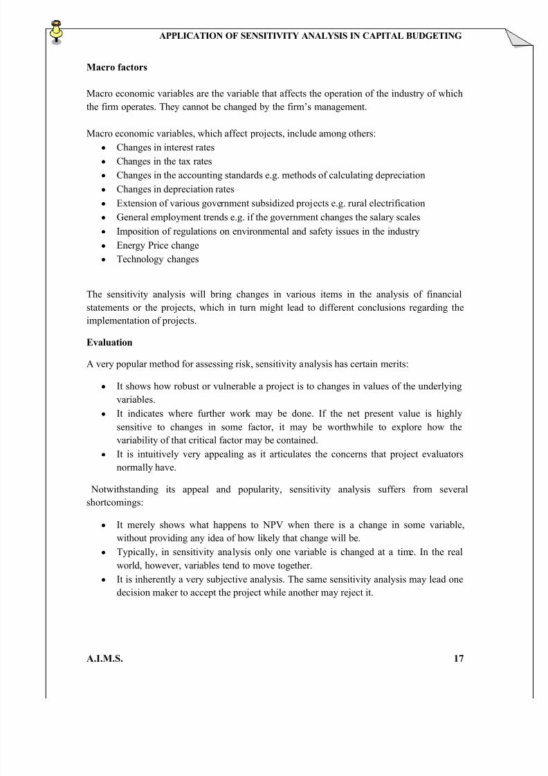
And, the Present Value of the Cash Flow of Year 1 at the discount rate 15 % would be:
PV of Cash flow of Year 1 = 136.488 / (1+0.15)
= Rs. 118.685 lakhs
Thus, the Pessimistic and Optimistic Values of the Cash Flow would be:
Discount
RatePessimistic Expected Optimistic
0.1 117.876 124.08 130.284
0.15 112.751 118.685 124.6195
Now, we consider the Sensitivity of the Cash Flow with respect to the Expenses entailed in
the production of the Batteries. For this purpose, we consider only the major Expenses
involved i.e. Raw Materials Cost, Employee Cost and Selling & Admin Expenses.
We take help of the Tornado Diagram so as to facilitate Decision making and ensure proper
allocation of the funds. We take the Pessimistic and the Optimistic Costs of the above
mentioned Expenses to draw the Tornado Diagram.
YEAR 1 Pessimistic Optimistic
Raw Materials 651.8484 589.7676
Employee Cost 99.6786 90.1854
Selling and Admin Expenses 139.3812 126.1068
But, these are the Pessimist and Optimistic values at the end of Year 1. So we need to
calculate the present values of these values.
Firstly, the values are calculated at 10% discount rate.
YEAR 1 Pessimistic Optimistic
Raw Materials 592.5818 536.1524
Employee Cost 90.61691 81.98673
Selling and Admin Expenses 126.7102 114.6425
The Diagram assumes Base Case Value to be the PV of the Cash flow at a discount rate of
10% i.e. 124.08.

8/9/2019 Application of Sensitivity Analysis
http://slidepdf.com/reader/full/application-of-sensitivity-analysis 28/42
APPLICATION OF SENSITIVIT ANAL SIS IN CAPITAL BUDGETING
A.I.M.S. 28
Here, the Pessi istic View suggests more expenses whereas the Optimistic view suggests
fewer expenses.
And now, we calculate the values at 15% discount rate.
YEAR 1 Pessi isti Opti isti
Raw Materials 566.81739 512.84139
E pl ee Cost 86.677043 78.422087
Selli and Admin
E penses
121.20104 109.65809
And, we assume Base Case Value to be the PV of the Cash f low at a discount rate of 15% i.e.
118.685.
0 100 200 300 400 500 600 700
R aw Mater ials
mployee Cost
Selling and Admin¡
xpenses
Pessimistic
Optimistic
0 100 200 300 400 500 600
R aw Mater ials
¡
mployee Cost
Selling and Admin¡
xpenses
Pessimistic
Optimistic

8/9/2019 Application of Sensitivity Analysis
http://slidepdf.com/reader/full/application-of-sensitivity-analysis 29/42
APPLICATION OF SENSITIVITY ANALYSIS IN CAPITAL BUDGETING
A.I.M.S. 29
Now, we need to analyse the 2 Tornado Diagrams so as to make decisions regarding the
expenses and find the better option amongst the 2 present values of the cash flow available.
We thus observe that the Raw materials Cost is almost similar in both the cases. But the
Pessimistic Cost i.e. more Expenses is more significant in both the cases. This is in line with
the market conditions generally where the raw materials costs grow. The Employee Cost in both the diagrams shows significance of the Optimistic view i.e. less expenses. So we can say
that the Employee Cost is manageable and may be according to our predictions for the 1st
year. The Selling and Admin Expenses show dominance of the optimistic view i.e. less
expenses. But, in the 2nd
diagram where we take the discount rate as 15%, the pessimistic cost
just comes into picture above the base value i.e. the cash flow value.
So, overall we can predict that if we look for the Raw Materials Cost, Employee Cost as well
as Selling and Admin Expenses then the 10% discounting factor is more suitable as it
provides more cash flow which is beneficial for the organisation.
Now, we move on to forecast for the Cash Flow of Year 2.
Again, we expect the Sales to increase 20% for Year 2. Therefore, Net Sales for Year 2
would be calculated as:
Net Sales (Year 2) = Net Sales (Year 1) + 0.20 x Net Sales (Year 1)
= 1028.796 + 0.20 x 1028.796
= 1234.55
Thus, Net Sales for Year 2 is Rs. 1234.55 lakhs.
We now forecast the Income and the Expenses of the unit for year 2 by using % of Sales
method as done earlier. Again the Cash Flow from the previous year is added to the Income
but, it does not play any part in the calculation of the Cash flow for Year 2.
% of SalesYear 2(Expected)
(Rs. Lakhs)
Income
Net Sales 1234.555
Other Income 0.24% 2.952
Cash Flow from Previous
Year 136.488
Total Income 1373.995
8/9/2019 Application of Sensitivity Analysis
http://slidepdf.com/reader/full/application-of-sensitivity-analysis 30/42
APPLICATION OF SENSITIVITY ANALYSIS IN CAPITAL BUDGETING
A.I.M.S. 30
Expenses
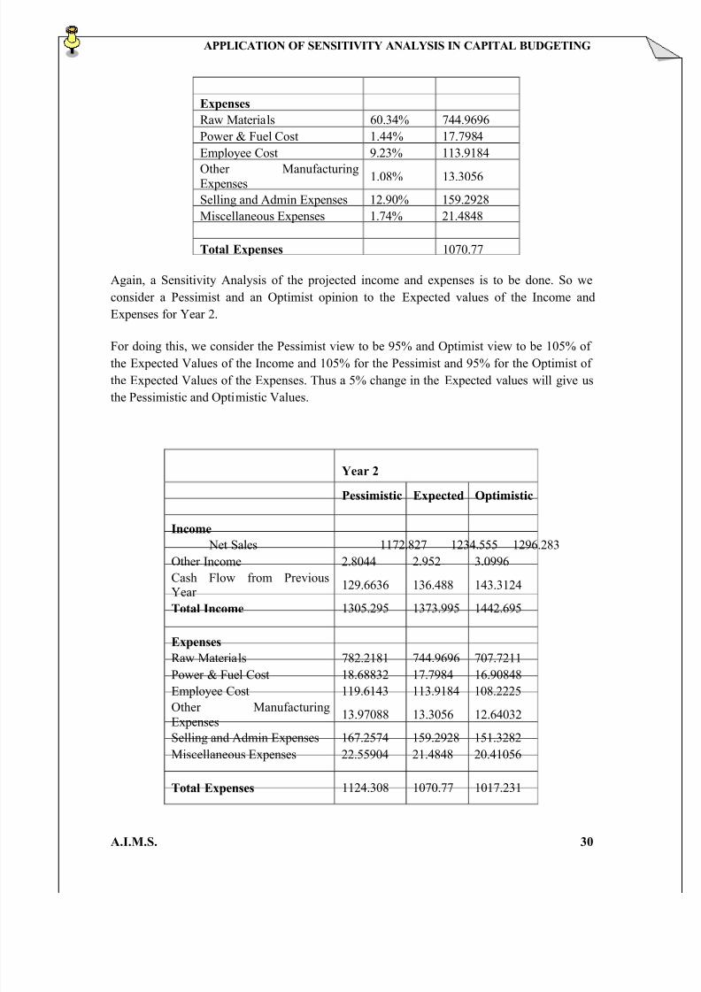
Raw Materials 60.34% 744.9696
Power & Fuel Cost 1.44% 17.7984
Employee Cost 9.23% 113.9184
Other ManufacturingExpenses 1.08% 13.3056
Selling and Admin Expenses 12.90% 159.2928
Miscellaneous Expenses 1.74% 21.4848
Total Expenses 1070.77
Again, a Sensitivity Analysis of the projected income and expenses is to be done. So we
consider a Pessimist and an Optimist opinion to the Expected values of the Income and
Expenses for Year 2.
For doing this, we consider the Pessimist view to be 95% and Optimist view to be 105% of the Expected Values of the Income and 105% for the Pessimist and 95% for the Optimist of
the Expected Values of the Expenses. Thus a 5% change in the Expected values will give us
the Pessimistic and Optimistic Values.
Year 2
Pessimistic Expected Optimistic
Income
Net Sales 1172.827 1234.555 1296.283
Other Income 2.8044 2.952 3.0996
Cash Flow from PreviousYear
129.6636 136.488 143.3124
Total Income 1305.295 1373.995 1442.695
Expenses
Raw Materials 782.2181 744.9696 707.7211
Power & Fuel Cost 18.68832 17.7984 16.90848
Employee Cost 119.6143 113.9184 108.2225Other Manufacturing
Expenses13.97088 13.3056 12.64032
Selling and Admin Expenses 167.2574 159.2928 151.3282
Miscellaneous Expenses 22.55904 21.4848 20.41056
Total Expenses 1124.308 1070.77 1017.231

8/9/2019 Application of Sensitivity Analysis
http://slidepdf.com/reader/full/application-of-sensitivity-analysis 31/42
APPLICATION OF SENSITIVITY ANALYSIS IN CAPITAL BUDGETING
A.I.M.S. 31
The Cash Flow from the Unit for Year 2 is calculated as:
Cash Flow of the Unit = Income ± Expenses
= Net Sales ± Total Expenses
= 1234.55 ± 1070.77
= Rs. 163.78 lakhs
Thus, the Cash flow of the Unit for Year 2 would be Rs. 163.78 lakhs.
Now, the Present Value of the Cash Flow of Year 2 at the discount rate 10 % would be:
PV of Cash flow of Year 2 = 163.78 / (1+0.10)
= Rs. 135.36 lakhs
And, the Present Value of the Cash Flow of Year 2 at the discount rate 15 % would be:
PV of Cash flow of Year 2 = 163.78 / (1+0.15)
= Rs. 123.845 lakhs
Thus, the Pessimistic and Optimistic Values of the Cash Flow would be:
Discount
Rate
Pessimistic Expected Optimistic
0.1 128.592 135.36 142.128
0.15 117.653 123.845 130.037
Again, we consider the Sensitivity of the Cash Flow with respect to the Expenses entailed in
the production of the Batteries. For this purpose, we consider only the major Expenses
involved i.e. Raw Materials Cost, Employee Cost and Selling & Admin Expenses.
We take help of the Tornado Diagram so as to facilitate Decision making and ensure proper
allocation of the funds. We take the Pessimistic and the Optimistic Costs of the above
mentioned Expenses to draw the Tornado Diagram.
YEAR 2 Pessimistic Optimistic
Raw Materials 782.218 707.721
Employee Cost 119.614 108.222
Selling and Admin Expenses 167.257 151.328
But, these are the Pessimist and Optimistic values at the end of Year 2. So we need to
calculate the present values of these values.

8/9/2019 Application of Sensitivity Analysis
http://slidepdf.com/reader/full/application-of-sensitivity-analysis 32/42
APPLICATION OF SENSITIVITY ANALYSIS IN CAPITAL BUDGETING
A.I.M.S. 32
Firstly, the values are calculated at 10% discount rate.
YEAR 2 Pessimisti Optimisti
Raw Materials 646.461 584.893
Employee Cost 98.854 89.439
Selling and Admin E penses 138.228 125.064
The Diagram assumes Base Case Value to be the PV of the Cash f low at a discount rate of
10% i.e. 135.36.
And now, we calculate the values at 15% discount rate.
YEAR 2 Pessimisti Optimisti
Raw Materials 591.469 535.138
Employee Cost 90.445 81.831
Selling and Admin
E penses126.47 114.425
And now, we assume Base Case Value to be the PV of the Cash f low at a discount rate of
15% i.e. 123.845.
0 100 200 300 400 500 600 700
R aw Mater ials
¢
mployee Cost
Selling and Admin£
xpenses
Pessimistic
Optimistic

8/9/2019 Application of Sensitivity Analysis
http://slidepdf.com/reader/full/application-of-sensitivity-analysis 33/42
APPLICATION OF SENSITIVITY ANALYSIS IN CAPITAL BUDGETING
A.I.M.S. 33
Now, we analyse the 2 Tornado Diagrams so as to make decisions regarding the expenses and
f ind the better option amongst the 2 present values of the cash f low available for Year 2.
We observe that the raw mater ials Cost, the mployee Cost as well as Selling and Admin
xpenses show similar trends at the 10% and 15% discount rates.The R aw mater ials cost
shows dominance of the pessimistic view i.e. more expenses whereas the mployee cost and
Selling and Admin xpenses shows dominance of Optimistic view i.e. less expenses.
So we can conclude that we can take any of the discount rates but the 10% discount rate isa
better option as it provides more cash f low in Year 2.
Now, we move on to forecast for the Cash Flow of Year 3.
Again, we expect the Sales to increase 20% for Year 3. Therefore, Net Sales for Year 3
would be calculated as:
Net Sales (Year 3) = Net Sales (Year 2) + 0.20 x Net Sales (Year 2)
= 1234.55 + 0.20 x 1234.55
= 1481.466
Thus, Net Sales for Year 3 is R s. 1481.466 lakhs.
0 100 200 300 400 500 600 700
R aw Mater ials
¤
mployee Cost
Selling and Admin¥
xpenses
Pessimistic
Optimistic
8/9/2019 Application of Sensitivity Analysis
http://slidepdf.com/reader/full/application-of-sensitivity-analysis 34/42
APPLICATION OF SENSITIVITY ANALYSIS IN CAPITAL BUDGETING
A.I.M.S. 34
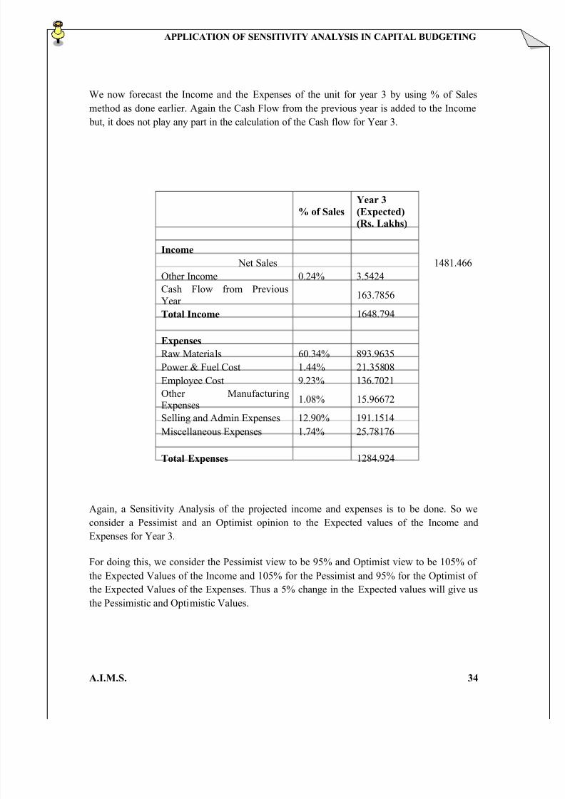
We now forecast the Income and the Expenses of the unit for year 3 by using % of Sales
method as done earlier. Again the Cash Flow from the previous year is added to the Income
but, it does not play any part in the calculation of the Cash flow for Year 3.
% of Sales
Year 3
(Expected)
(Rs. Lakhs)
Income
Net Sales 1481.466
Other Income 0.24% 3.5424Cash Flow from Previous
Year 163.7856
Total Income 1648.794
Expenses
Raw Materials 60.34% 893.9635
Power & Fuel Cost 1.44% 21.35808
Employee Cost 9.23% 136.7021
Other ManufacturingExpenses
1.08% 15.96672
Selling and Admin Expenses 12.90% 191.1514Miscellaneous Expenses 1.74% 25.78176
Total Expenses 1284.924
Again, a Sensitivity Analysis of the projected income and expenses is to be done. So we
consider a Pessimist and an Optimist opinion to the Expected values of the Income and
Expenses for Year 3.
For doing this, we consider the Pessimist view to be 95% and Optimist view to be 105% of
the Expected Values of the Income and 105% for the Pessimist and 95% for the Optimist of
the Expected Values of the Expenses. Thus a 5% change in the Expected values will give us
the Pessimistic and Optimistic Values.

8/9/2019 Application of Sensitivity Analysis
http://slidepdf.com/reader/full/application-of-sensitivity-analysis 35/42
APPLICATION OF SENSITIVITY ANALYSIS IN CAPITAL BUDGETING
A.I.M.S. 35
Year 3
Pessimistic Expected Optimistic
Income
Net Sales 1407.393 1481.466 1555.54Other Income 3.36528 3.5424 3.71952
Cash Flow from Previous
Year 155.5963 163.7856 171.9749
Total Income 1566.355 1648.794 1731.234
Expenses
Raw Materials 938.6617 893.9635 849.2653
Power & Fuel Cost 22.42598 21.35808 20.29018
Employee Cost 143.5372 136.7021 129.867
Other Manufacturing
Expenses16.76506 15.96672 15.16838
Selling and Admin Expenses 200.7089 191.1514 181.5938
Miscellaneous Expenses 27.07085 25.78176 24.49267
Total Expenses 1349.17 1284.924 1220.677
The Cash Flow from the Unit for Year 3 is calculated as:
Cash Flow of the Unit = Income ± Expenses
= Net Sales ± Total Expenses
= 1481.466 ± 1284.924
= Rs. 196.542 lakhs
Thus, the Cash flow of the Unit for Year 3 would be Rs. 196.542 lakhs.
Now, the Present Value of the Cash Flow of Year 3 at the discount rate 10 % would be:
PV of Cash flow of Year 3 = 196.542 / (1+0.10)
= Rs. 147.655 lakhs
And, the Present Value of the Cash Flow of Year 3 at the discount rate 15 % would be:
PV of Cash flow of Year 3 = 196.542 / (1+0.15)
= Rs. 129.23 lakhs

8/9/2019 Application of Sensitivity Analysis
http://slidepdf.com/reader/full/application-of-sensitivity-analysis 36/42
APPLICATION OF SENSITIVITY ANALYSIS IN CAPITAL BUDGETING
A.I.M.S. 36
Thus, the Pessimistic and Optimistic Values of the Cash Flow would be:
Discount
RatePessimistic Expected Optimistic
0.1 140.282 147.665 155.048
0.15 122.768 129.23 135.691
Again, we consider the Sensitivity of the Cash Flow with respect to the Expenses entailed in
the production of the Batteries. For this purpose, we consider only the major Expenses
involved i.e. Raw Materials Cost, Employee Cost and Selling & Admin Expenses.
We take help of the Tornado Diagram so as to facilitate Decision making and ensure proper
allocation of the funds. We take the Pessimistic and the Optimistic Costs of the above
mentioned Expenses to draw the Tornado Diagram.
YEAR 3 Pessimistic Optimistic
Raw Materials 938.661 849.265Employee Cost 143.537 129.866
Selling and Admin Expenses 200.708 181.593
But, these are the Pessimist and Optimistic values at the end of Year 3. So we need to
calculate the present values of these values.
Firstly, the values are calculated at 10% discount rate.
YEAR 3 Pessimistic Optimistic
Raw Materials 705.2299 638.0654
Employee Cost 107.8415 97.57025
Selling and Admin Expenses 150.7949 136.4335
The Diagram assumes Base Case Value to be the PV of the Cash flow at a discount rate of
10% i.e. 147.665.

8/9/2019 Application of Sensitivity Analysis
http://slidepdf.com/reader/full/application-of-sensitivity-analysis 37/42
APPLICATION OF SENSITIVITY ANALYSIS IN CAPITAL BUDGETING
A.I.M.S. 37
And now, we calculate the values at 15% discount rate.
YEAR 3 Pessimisti Optimisti
Raw Materials 617.18484 558.40552
Employee Cost 94.377907 85.389003
Selling and Admin
E penses 131.96877 119.40035
And now, we assume Base Case Value to be the PV of the Cash f low at a discount rate of
15% i.e. 129.23.
Now, we analyse the 2 Tornado Diagrams so as to make decisions regarding the expenses and
f ind the better option amongst the 2 present values of the cash f low available for Year 3.
0 100 200 300 400 500 600 700 800
R aw Mater ials
¦
mployee Cost
Selling and Admin§
xpenses
Pessimistic
Optimistic
0 100 200 300 400 500 600 700
R aw Mater ials
mployee Cost
Selling and Admin xpenses
Pessimistic
Optimistic

8/9/2019 Application of Sensitivity Analysis
http://slidepdf.com/reader/full/application-of-sensitivity-analysis 38/42
APPLICATION OF SENSITIVITY ANALYSIS IN CAPITAL BUDGETING
A.I.M.S. 38
We observe that all the Expenses i.e. Raw materials cost, Employee cost and Selling and
Admin Expenses show similar trends for both the discount rates. Thus, we can conclude that
Year 3 follows the same trend as in Year 2 by increase of raw materials cost and decrease of
Employee Cost and Selling % Admin Expenses with the only exception that the Selling and
Admin Expenses have values on either side of the base case value. This states that the Selling
and Admin Expenses will depend upon the value which would hold true in year 3 i.e. the pessimistic or the Optimistic value. Thus, again a discount rate of 10% can be taken as it
provides more cash flows to the unit.
Thus, to conclude overall for the unit for the 3 years we can say that the cash flows generated
would be in direct relation to the raw material cost, employee cost and the selling and admin
expenses which form the major part of any business. Also, the difference in the discounting
factor for the present value does not have much effect on the present values of the cash flows
and hence, we can say that the trends in cash flows and expenses are independent of the
discounting factor. Thus, we can take the discounting rate as 10% for more cash flows.
Speaking about the trend in expenses, the Raw material costs shows an increasing trend over
the next 3 years for the unit. But, the gap between the pessimistic view and the optimistic
view seems to be reducing over the years. The Employee cost may increase over the years
and may bring down the value of cash flows down but if they remain optimistic as shown in
all the diagrams may help in bringing in more cash flows. The Selling and Admin Expenses
show a stable trend in these 3 forecasted years but the pessimist cost just seems to come into
picture in the last year of forecasting and if a similar trend continues, may bring down the
cash flows in future.

8/9/2019 Application of Sensitivity Analysis
http://slidepdf.com/reader/full/application-of-sensitivity-analysis 39/42
APPLICATION OF SENSITIVITY ANALYSIS IN CAPITAL BUDGETING
A.I.M.S. 39
5.CONCLUSION

8/9/2019 Application of Sensitivity Analysis
http://slidepdf.com/reader/full/application-of-sensitivity-analysis 40/42
APPLICATION OF SENSITIVITY ANALYSIS IN CAPITAL BUDGETING
A.I.M.S. 40
CONCLUSION
The project briefly describes the risks involved and the techniques for analysis of these risks that play a major role in Capital Budgeting of a company.
A detailed study of some of these techniques such as Sensitivity Analysis and
Scenario Analysis is done and the practical approach mostly followed by the corporate is
looked into in detail.
A hypothetical company is selected and a Sensitivity Analysis is done of its
production unit for a period of three years so as to find the major expenses and income that
affect the cash flows of the production unit of the company. The present value of these cash
flows is generated and checked against the optimistic and pessimistic values found by the
Sensitivity Analysis.
A Tornado Diagram is drawn in support of the data obtained and analysis regarding
the effects of the major expenses is done. The analysis suggests that out of the major
expenses raw materials cost is the most dominant factor affecting the cash flows and this has
the capability of making or breaking a cash flow for a particular year. The Selling and Admin
expenses tend to increase but at a very slow and steady pace and are manageable. The
Employee Cost is the most stable cost of the unit for the selected period. But, the diagram
suggests that if it is controlled may result into higher cash flows for the unit.
All this leads to a conclusion that risk analysis is a major part of Capital budgeting as
risk is an integral part of a business. Estimating this risk efficiently and effectively plays asignificant role in the process of Capital Budgeting.

8/9/2019 Application of Sensitivity Analysis
http://slidepdf.com/reader/full/application-of-sensitivity-analysis 41/42
APPLICATION OF SENSITIVITY ANALYSIS IN CAPITAL BUDGETING
A.I.M.S. 41
6. BIBLIOGRAPHY

8/9/2019 Application of Sensitivity Analysis
http://slidepdf.com/reader/full/application-of-sensitivity-analysis 42/42
APPLICATION OF SENSITIVITY ANALYSIS IN CAPITAL BUDGETING
BIBLIOGRAPHY
BOOKS:
Financial Management ± Prasanna Chandra
Projects ±Prasanna Chandra
Project Finance
WEBSITES:
www.google.com
www.wikipedia.com
www.investopedia.com
www.howstuffworks.com
www.questia.com
www.cambridge.org