APPLICATION OF GAUSS ALGORITHM AND MONTE CARLO SIMULATION

TO THE IDENTIFICATION OF AQUIFER PARAMETERS

By Timothy J. Durbin

U.S. GEOLOGICAL SURVEY

Open-File Report 81-688

mCOo oo

Sacramento, California 1983

UNITED STATES DEPARTMENT OF THE INTERIOR

JAMES G. WATT, SECRETARY

GEOLOGICAL SURVEY

Dallas L. Peck, Director

For additional information write to:

District Chief U.S. Geological Survey Federak Building, Room W-2235 2800 Cottage Way Sacramento, CA 95825

Copies of this report can be purchased from:

Open-File Services Section Western Distribution Branch U.S. Geological Survey Box 25424, Federal Center Denver, CO 80225 Telephone: (303) 234-5888

CONTENTS

• PageAbstract - — ----- — - —— — - —— - — — - — —— -»__- — — _ —— - — —— —— —— __ — —— __ jIntroduction —--——-————--.--—----——-—-—--——-————-———-—— 2Identification problem -—--—-—-— —— ——— -——-————-—-——————---- 3

Ground-water model ——— ——————————— ——— ————— —— ———— ————— 3Objective function ————————————— ———— ————— —— — ——————— — 4Gauss optimization technique —— — —— — —— —————————-——————— 5Levenberg parameter - —— ——————— ———————————— ————————— ——— 6

Parameter discretization -——'-—- ————--—--—————-———--————— 7Numerical example --——— — --——-------—- — -———-——-———————-— 9Effects of data errors -——-———----——- — --- ——————-—-——-——- nSummary and conclusions — ——————————— ——— ———— ————— —————————— 14References cited --———-—————--———---—-——————-——-—————- 15

ILLUSTRATIONS

Page Figures 1-5. Maps showing:

1. Ground-water subbasins, generalized geology, and steady-state water-level contours for the upper Coachella Valley ground-water basin, California — —— ---- — —— - — —— — - —— —— — --- — --- 17

2. Element layout for the model of the WhitewaterRiver and Garnet Hill subbasins ---- — — ———— —— - 18

3. Geographic distribution of natural recharge toWhitewater River and Garnet Hill subbasins -———-- 19

4. Subdomains and water-level points used incomputing optimum transmissivity from steady- state conditions -——- — --———-———---- ———— 20

5. Optimum transmissivity obtained by objectively adjusting large-scale variations of transmissivity and by subjectively adjusting small-scale variations of transmissivity —— —— --- 21

6. Graph of convergence of the Gauss optimization techniquefor different search radii, r ———————————————————- 22

TABLES

Page Table 1. Optimum surrogate parameters computed from field data -—————— 23

2. Summary statistics an random recharge estimates ——-—---———— 243. Optimum surrogate parameter values computed using random

recharge estimates --—-—-—--—----—--—---————————--— 254. Hydraulic-head responses predicted with model using optimum

surrogate parameters computed using random recharge estimates ---——--——-—----—---—-——-———- —— — -——-——— 26

CONVERSION FACTORS

In this report measurements are given in International System of Units. Conversion factors from International System of Units to inch-pound units are given below.

Multiply By To obtainhmr3 (cubic hectometers) 810.7 acre-ft (acre-feet)km (kilometers) .6214 mi (miles)m (meters) 0.3048 ft (feet)m2 /s (meters squared per second) 10.76 ft2/s (feet squared per

second) m3 /s (cubic meters per second) 35.31 fts/s (cubic feet per

second)

ALTITUDE DATUM

National Geodetic Vertical Datum of 1929 (NGVD of 1929): A geodetic datum derived from a general adjustment of the first-order level nets of both the United States and Canada, formerly called mean sea level.

APPLICATION OF GAUSS ALGORITHM AND MONTE CARLO SIMULATION

TO THE IDENTIFICATION OF AQUIFER PARAMETERS

By Timothy J. Durbin

ABSTRACT

The Gauss optimization technique can be used to identify the parameters of a model of a ground-water system for which the parameter-identification problem is formulated as a least-squares comparison between the response of the prototype and the response of the model. Unavoidable uncertainty in the true stress on the prototype and in the true response of the prototype to that stress will introduce errors into the parameter-identification problem. These errors are subsequently transferred to the prediction problem. The fit of the model to the data that are used to identify parameters is not a good indicator of these errors. A Monte Carlo simulation of the parameter-identification problem and of the prediction problem can be used, however, to evaluate the effects on water-level predictions of errors in the recharge (and pumpage) data used in the parameter-identification problem.

INTRODUCTION

Some important problems encountered in simulating the behavior of ground-water systems can be classified as either prediction problems or parameter-identification problems. The prediction problem is to estimate the response of the prototype to specific inputs by using a mathematical model of the system. The parameter-identification problem is to find an optimum set of parameters for the model from concurrent prototypical input and output obser­ vations. In the parameter-identification problem, the mathematical structure of the equation characterizing the prototype is given, but the specific values of the coefficients of the equation, the initial conditions, or the boundary conditions are unknown. These unknowns are the parameters in the parameter- identification problem.

Current methods of parameter identification can be divided into direct or indirect methods (Neuman, 1973). The direct methods treat the model param­ eters as dependent variables in a formal boundary value problem (Stallman, 1956; Nelson, 1968; Nelson and McCollum, 1969; Kleinecke, 1971; Emsellem and de Marsily, 1971; Sagar, 1973; and Frind and Finder, 1973). With indirect methods, existing estimates of the parameters are improved iteratively (Kruger, 1961; Jacquard and Jain, 1965; Jahns, 1966; Vemuri and Karplus, 1969; Coats and others, 1970; Slater and Durrer, 1971; Yeh and Tauxe, 1971; Lovell, 1971; Bruch and others, 197A; and McLaughlin, 1974). The indirect methods are generally computationally less efficient than the direct methods. However, the indirect methods are probably more flexible with respect to the different types of models that can be used.

The Gauss optimization technique (Gauss, cited in Wilde and Beightler, 1967, p. 299) is an indirect method of parameter identification. The applica­ tion of this technique to the identification of the parameters of a ground- water model is demonstrated in this paper. In addition, the effects on the modeling process of errors in the input observations are analyzed. The modeling process includes both the identification of the model parameters and the use of the model to predict the response of the prototype to specific inputs. Unavoidable uncertainty in the true stress on the prototype and in the true response of the prototype to that stress will introduce errors into the parameter-identification problem. These errors are subsequently transferred to the prediction problem.

The Gauss technique has been used by others to identify the parameters for models of oil reservoirs (Jahns, 1966) and ground-water systems (McLaughlin, 1974). The originality of the work in this paper is chiefly in the method of parameter discretization, the application of the Gauss technique to a field case, and the analyses of the effects of data errors.

In particular applications, the mathematical equations of ground-water flow only approximately characterize the properties of the prototype. This lack of exact equivalency between the model and the prototype often leads to bias in the parameter estimates. This problem, however, is not addressed in this paper.

IDENTIFICATION PROBLEM

Ground-Water Model

The first step in the identification of parameters is to specify the model to be used and to isolate the unknown parameters. A partial differen­ tial equation that describes the steady flow of ground water in a two- dimensional isotropic aquifer is

Iz <?& + ry <Ti> + o = ° <»where Q is the strength of a source or sink,

Q = I Qw (xi ,yi ) 6 (x-x ) 6 (y-y^ (2) i

and h is the hydraulic head, Q is the rate of recharge or withdrawl at point (x.,y.)> T is the transmissivity, and 6 is the Dirac delta function.

Equation 1 is to be solved in a domain Q, which is enclosed by the boundary f = r 1UF2 . The boundary conditions are the specified head boundary condition

h = £1 on T! (3)

and the specified flux boundary condition

3h - t ™ r - £2 on T2

where 3h/8n is the outward-pointing, normal derivative on f2> and £j_ and £2 are prescribed functions of location on r\ and r2 .

The Galerkin-finite element method is used to solve equation 1. The solution scheme follows Finder and Frind (1972), except that linear shape functions are defined on triangular elements .

Objective Function

The second step in the identification of parameters is to select an ob­ jective function that compares the model response and the prototype response.

Let 0 E (81, 82,..., 8.) be a vector of the parameters to be identified.

A least-squares objective function is given by

M •P = I [h. - h.(8)] 2

where h. is the measured hydraulic head at the data point (x.,y.)r h. is the

computed hydraulic head at the data point, and M is the number of data points.-Jf «• rT «• f

Let the vector 6 H (6j, 62,..., 6^) be a particular point in an unbounded

feasible region such that the value of the objective function is smaller than at any other point in the feasible region (McLaughlin, 1974, describes the application of the Gauss algorithm for the case of a closed feasible region).

Jw

The members of 8 are called the unconstrained optimum parameters.

A necessary condition at 8 resulting normal equations are

is that the gradient of P vanish there. The

3Paei = 0 i = 1, 2,..., K (6)

orJT[h - h(8)] = 0 (7)

where

J ZL

3n\ 3^^

38 1

3h2

38!

3hM

36 !

^ Q <\ f\oo2 O®Y

3h2 3h2^i£i <^ ACU2 O\J^r

3hM 3hMM. . . Mo f\ <\ f\002 Ouv

is the Jacobian matrix, h H (hi, h2,..., hM ) is a vector is measured hydrau-* A ~ " T n lie heads and h H (hi, h2,..., h-,) is a vector of computed hydraulic heads.

Gauss Optimization Technique

The third step in the identification of parameters is to select an algorithm for adjusting the parameters so that the objective function is minimized. Equation 7 represents a system of simultaneous equations that are nonlinear in the parameters. This system can be solved by the Gauss technique (Gauss, cited in Wilde and Beightler, 1967, p. 299; Hartley, 1961; Marquardt,

* 1963; Jahns, 1966; and McLaughlin, 1974), which starts at a point close to 6and proceeds stepwise toward a minimum by successive improvements.

<s

In the Gauss technique, equation 7 is linearized by expanding h(6) in a Taylor series about the current trial values of 6 and by retaining only the

linear terms. The substitution of the Taylor series representation of h(6) into equation 7 yields

(J^VjJ^Ae = (J^Vth - hCe^ 1 )] (8)

where the superscript j-1 designates quantities evaluated at the last trial- T

values and A8 =. (A8i, A62 ,..., A8V ) is the vector of parameter corrections.lv

The updated values of the parameters at the jth iteration are given by

eJ = e-^" 1 + A0 (9)«ju

Successive improvements are made until 6 converges to 8 , where convergence is defined as follows: If the value of the objective function has decreased at each of the last N iterations, and if the maximum change in the value of the objective function at successive iterates is less than some specified value,

JU

convergence to 8 is declared. This definition is subjective, and most likely the definition will have to be modified in particular applications.

The objective function is typically polymodal (Jahns, 1966), and in practice, only a local minimum of the objective function can be found. Experience with the Gauss algorithm, however, seems to indicate that, for the steady-state form of the parameter-identification problem, the objective function tends to be unimodal as fewer measured water-level points are used and as fewer parameters are considered.

Levenberg Parameter

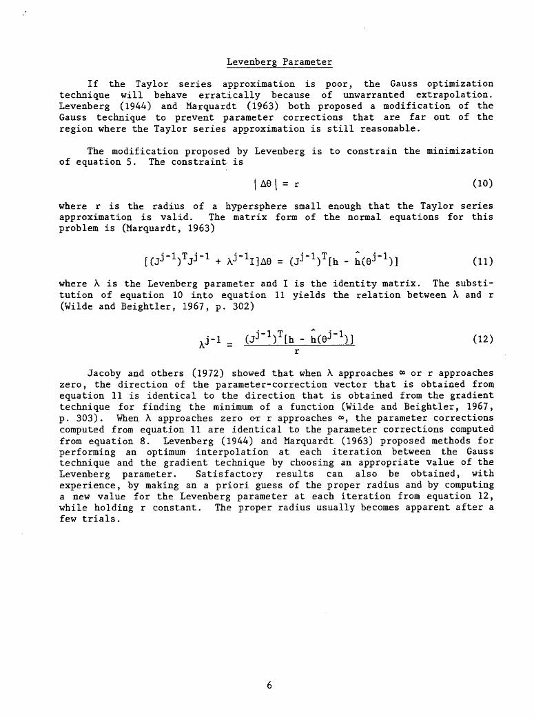
If the Taylor series approximation is poor, the Gauss optimization technique will behave erratically because of unwarranted extrapolation. Levenberg (1944) and Marquardt (1963) both proposed a modification of the Gauss technique to prevent parameter corrections that are far out of the region where the Taylor series approximation is still reasonable.

The modification proposed by Levenberg is to constrain the minimization of equation 5. The constraint is

j A6 \ = r (10)

where r is the radius of a hypersphere small enough that the Taylor series approximation is valid. The matrix form of the normal equations for this problem is (Marquardt, 1963)

[(J^Vj-3"" 1 + V^IjAe = (Jj " 1 ) T [h - h(6j " 1 )] (11)

where A. is the Levenberg parameter and I is the identity matrix. The substi­ tution of equation 10 into equation 11 yields the relation between A. and r (Wilde and Beightler, 1967, p. 302)

1 )] (12)

Jacoby and others (1972) showed that when A. approaches » or r approaches zero, the direction of the parameter-correction vector that is obtained from equation 11 is identical to the direction that is obtained from the gradient technique for finding the minimum of a function (Wilde and Beightler, 1967, p. 303). When A approaches zero or r approaches », the parameter corrections computed from equation 11 are identical to the parameter corrections computed from equation 8. Levenberg (1944) and Marquardt (1963) proposed methods for performing an optimum interpolation at each iteration between the Gauss technique and the gradient technique by choosing an appropriate value of the Levenberg parameter. Satisfactory results can also be obtained, with experience, by making an a priori guess of the proper radius and by computing a new value for the Levenberg parameter at each iteration from equation 12, while holding r constant. The proper radius usually becomes apparent after a few trials.

PARAMETER DISCRETIZATION

In discussing ground-water models the question of the scale of parameter discretization invariably arises. But before the question can be considered, the scale of a model needs to be defined. The definition used here is that the scale of a two-dimensional ground-water model is the size of the area over which the system parameters are considered to homogeneous.

Two aspects of model scale are to be considered. The first deals with the predictions that are made with a model. Consider the effect on computed hydraulic heads of random perturbations in spatially discretized system parameters. At some very small scale of discretizaton, these random perturbations will not significantly affect the computed hydraulic heads (Freeze, 1975). However, as the scale of parameter discretization is increased, at some point the random perturbations in the system parameters will significantly affect the computed hydraulic heads. The scale at which this occurs depends on the definition of a significant effect for a particular situation.

The second aspect of the scale of a ground-water model deals with the parameter-identification problem. Consider the effect on the parameter- identification problem of random errors in the measured water levels or in the estimates of the prototype pumpage and recharge. For example, the actual transmissivity of an aquifer might be uniform, but geographic variations of the hydraulic-head gradient occur because of variations in pumpage and recharge. Because of errors in the estimation of pumpage and recharge, however, the variation of the hydraulic-head gradient is interpreted as being caused in part by geographic variations of transmissivity. Similarly, errors in the estimation of hydraulic-head gradient from water-level data might also lead to the interpretation that transmissivity varies geographically. If, when considering the ground-water basin as a whole, errors in measured water levels, pumpage, and recharge are distributed with zero mean, at some very large scale of parameter discretization, these variations have very little effect on the parameter-identification problem. As the scale of parameter discretization is reduced, however, these errors may significantly affect the estimates of the system parameters.

Herein lies the dichotomy. We would like a small scale of parameter discretization for making predictions with the model. We would also like a large scale of parameter discretization for identifying the system parameters.

This disparity can be ameliorated somewhat by aggregating small-scale heterogeneity into surrogate parameters that are heterogeneous on a larger scale. In a practical sense, the small-scale heterogeneity would be at the level of the area of an element used in the finite-element solution of equation 1. The surrogate parameters would represent the aggregation of a group of elements.

The surrogate parameters are introduced into the parameter-identification problem by dividing the domain Q into K subdomains UK (j = 1, 2,..., K). A subdomain is made up of one or more elements. The ̂ geographic variation oftransmissivity in u). is given by

*J

T. = T..°6. (13) i ij J

where T..° is a prescribed base transmissivity for the element i in the

subdomain j, and 8. is a surrogate parameter. The surrogate parameter is a dimensionless factor that multiplies the base transmissivity for each element in a subdomain. The parameter identification problem is then to identify thesurrogate parameters that minimize the objective function, and the optimum

* transmissivity T. is given by the relation

T.* = T..°8.* (14) i ij J

The relative distribution of transmissivity within a subdomain is fixed by the prescription T..°. The actual distribution of transmissivity within a

IJ JL

subdomain is fixed by the identification of 6. . The number and size of%J

subdomains to be used and the distribution of T..° within each subdomain is prescribed ad hoc. ^

In the prototype, there is usually little reason to expect that the distribution of transmissivity will not be continuous, except at faults or other geologic discontinuities. The terms "continuous" and "continuity," which have precise meaning in mathematics, are used loosely in the context of the model to mean that the transmissivity of adjacent elements do not differ much. With this definition in mind, the continuity of transmissivity within a subdomain can be assured by assigning proper values to T..°. But the

continuity of transmissivity across the boundaries of adjacent subdomains is not assured.

A strategy for obtaining a continuous distribution over the entire model domain is to use objective optimization for the large-scale variations of transmissivity and to use subjective optimization for the small-scalevariations. For each subdomain, an initial distribution of T..° is prescribedijthat is continuous within and between adjacent subdomains. Optimum values for the surrogate parameters are computed. The new distribution of transmissivity is likely to be discontinuous across the subdomain boundaries. This distribution is then subjectively smoothed to eliminate these discontinuities, and optimum values for the surrogate parameters are again computed. This procedure is repeated until a continuous distribution is obtained.

An important difficulty in the parameter identification problem is that it is virtually impossible to express subjective information in a generalized mathematical form. But the subjective information that is usually available to a hydrologist is important to the parameter-identification problem. An advantage of the above procedure for obtaining a continuous distribution of transmissivity is that it uses the digital computer for those parts of the problem that can be translated into an algorithm, while allowing the introduction of judgments and insights into the problem as they are required.

NUMERICAL EXAMPLE

The Gauss optimization technique was used to identify the distribution of transmissivity for a model of the Whitewater River and Garnet Hill subbasins of the upper Coachella Valley ground-water basin (fig. 1). This study area covers about 400 km2 . Ground water occurs in unconsolidated and moderately indurated alluvial deposits (Dutcher and Bader, 1963; Farrell, 1964; Proctor, 1968; and Tyley, 1974), which have a saturated thickness of as much as 900 m (Biehler, 1964). A fault in the study area acts as a barrier to ground-water movement; hydraulic-head differentials of as much as 100 m occur across the fault. The effect of the fault on ground-water movement was represented in the model (fig, 2) by low transmissivity in the elements along the fault.

Prior to 1946, the hydraulic heads in the upper Coachella Valley ground- water basin were in quasi-equilibrium with natural recharge. The principal source of natural recharge was the percolation from the channels of ephemeral and intermittent streams that cross the ground-water basin (fig. 3). Optimum transmissivity was computed for this condiiton. Hydraulic head measurements and estimates of natural recharge were obtained from Tyley (1974).

The model domain was divided into 16 subdomains (fig. 4). Initially

T..° = 4.2 x io~ 2 m2 /s for all elements in subdomains 1, 2, 3, 4, 5, and 6;

T..° = 9.3 x io" 5 m2 /s for all elements in subdomains 7, 8, 9, 10, and 11; and

T. .° = 7.0 x io" 3 m2 /s for all elements in subdomains 12, 13, 14, 15, and 16.1J JU

The optimum surrogate parameters 6 were computed (table 1), and the optimum*

transmissivities T. were plotted on a map of the study area. This plotrevealed discontinuities in the geographic distribution of transmissivity in areas where a continuous distribution reasonably would have been expected. Subjective adjustments were made to the transmissivities to remove these

*discontinuities. New values of 6 were computed (table 1). The corresponding

juvalues of T. were plotted, and the geographic distribution was examined for physical plausibility. These values (fig. 5) were accepted, and the parameter identification problem was completed.

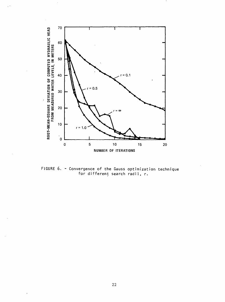
Figure 6 shows the root-mean-square deviation of the computed hydraulic head from the measured hydraulic head, at each iteration in the initial opti­ mization, for values of r equal to 0.1 (approaching a gradient step), 0.5, 1.0, and oo (the Gauss step). For r = °°, the initial rate of convergence is rapid, but at some points the search diverges at successive iterates. For r = 0.1, convergence is slow, but stable. For r = 1.0, the most rapid rate to final convergence is exhibited; convergence is obtained after about 15 iterations.

An appropriate question to ask at this point is: How good are the estimates of transmissivity for this ground-water basin? If we had a perfect model and perfect knowledge of the prototype recharge and water levels, then the calibration procedure should yield a very close approximation of the true prototype transmissivity. However, our model is only an approximation of the prototype, and we have imperfect knowledge of the prototype recharge and of the corresponding prototype response. As a consequence, the transmissivity estimates probably deviate from the true transmissivity, which leads u? back to the original question.

The approach that is often used is to examine the objective function value corresponding to the optimum parameters and also to examine the departure of the optimum parameters from subjective estimates of the optimum parameters. If the objective function and the parameter departures are within acceptable limits, the hydrologist accepts the parameter estimates. The inadequacy of this approach is chiefly in that it does not consider the effect of data errors on the parameter estimates.

A second approach that has been suggested, but seldom used in practice, is split-sample testing. Split-sample testing consists of organizing the available field data into two parts, each representing a different historical period. Optimum parameter estimates are computed using one part of the data. Then, the model is used to simulate conditions during the historical period represented by the second part of the data. The deviations of the computed hydraulic heads from the measured water levels for the second historical period are assumed to be a measure of the predictive reliablility of the model.

In many applications split-sample testing is a powerful statistical tool for evaluating models. When used to evaluate ground-water models, however, this technique often fails to provide useful information. This failure occurs because the available field data seldom can be divided into two independent samples.

The point of the above discussion is that a methodology for evaluating the predictive reliability of ground-water models is still in the developing stages. Attention will focus here on what the author considers to be a first step in developing approaches for evaluating ground-water models--conditional evaluations based on an assumed probability model of the occurence of errors in the independent variables. An unconditional evaluation would probably require the generation of additional information. Just how this information would be generated depends largely on the specifics of a particular situation. It might involve additional primary data collection, the use of independent parameter estimates from secondary data sources, or the application of subjective information through constrained regression, or through Bayesian estimation procedures.

10

EFFECTS OF DATA ERRORS

Measurements and sampling errors in the independent variables that are used to compute the optimum parameters are reflected in the deviation of the optimum parameters from the true parameters. If the optimum parameters are used in the model to make predictions of the response of the prototype to assumed future stresses, the predicted response will be in error. In the following paragraphs, a technique for analyzing these errors in the predicted response is demonstrated using the model of the upper Coachella Valley ground- water basin.

The upper Coachella Valley ground-water basin is being artificially recharged with imported water. Recharge operations began in 1973 when 9.2 hm3 of water was recharged from percolation ponds in the northern part of the ground-water basin (fig. 1). Annual recharge will most likely be increased until a maximum annual recharge of 75 hm3 is reached in about 1990. One effect of the recharge operation will be raised ground-water levels in wells. The maximum rise will occur when the hydraulic head in the ground-water basin reaches the steady-state values. Model predictions indicate that the maximum water-level rise, due only to the artificial recharge, will be about 350 m at the recharge site and about 180 m at Palm Springs, a major population center in the upper Coachella Valley (fig. 1). (Superimposed on the effect of artificial recharge is the effect of pumpage, which was not considered in the example.)

These water-level rises were computed from the model using the transmis- sivity estimates shown in figure 5. If different estimates of natural recharge had been used in the parameter-identification problem, different transmissivity estimates would have been obtained, and different predictions of the water-level response to artificial recharge would have been made. The independent variables of the parameter-identification problem are random variables, and transmissivity estimates and water-level predictions, which are functions of the independent variables, are also random variables. Conclu­ sions about the effects on the modeling process of errors in the independent variables should be based on the statistical nature of the transmissivity estimates and of water-level predictions. A Monte Carlo simulation (Benjamin and Cornell, 1970, p. 124) of the modeling process provides a method for examining the statistical nature of these quantities, in spite of data limitations in the real world, which preclude a direct examination. The method is described stepwise as follows:

Step 1: Random estimates of the local recharge rate were generated. These estimates were considered to come from log-normal distributions with means equal to the estimates used in the original numerical example (fig. 3) and coefficient of variation equal to 25 percent. The assumed distribution of the local recharge estimates was derived heuristically and is undoubtedly situationally specific.

11

Step 2: Transmissivity estimates were computed using the new recharge estimates obtained in step 1. Except for the new recharge estimates, the configuration of the parameter identification problem was as in the original numerical example. Identical subdomains and measured water levels were used. The relative geographic distribution of the transmissivity within subdomains was the same as shown in figure 5.

Step 3: The model was used to compute steady-state hydraulic head for artificial recharge. The transmissivity estimates from step 2 were used in the model for this step.

Steps 1 through 3 were repeated 20 times, and the results are given in tables 2, 3, and 4. The range, mean, and coefficient of variation of the generated natural-recharge estimates are given in table 2 for each recharge site. With reference to the parameter-identification problem, the surrogate parameter estimates and the root-mean-square deviation of computed hydraulic heads from measured water levels are given in table 3 for each execution of step 2. The mean coefficient of variation of the surrogate parameter estimates are also given in table 3 for each surrogate parameter. With reference to the prediction problem, the water levels at the recharge site and at Palm Springs are given in table 4, for each execution of step 3. Addition­ ally, the means and coefficients of variation of these water levels are given in table 4.

Initial values of surrogate parameters for the parameter-identification problem were, for each recharge data set, the values given in table 1, which gives the optimum surrogate parameters for the original numerical example. Although individual optimum-parameter values obtained from the Monte Carlo simulation deviate as much as 60 percent from initial values, the means of the various estimates of individual parameters are nearly identical to the values given in table 1. The coefficients of variation of these estimates range from 6 to 17 percent. The upper limit of this range is less than the coefficient of variation used in the generation of recharge estimates.

The magnitude of the deviation of the surrogate parameters tends to be related to the magnitude of the deviation of the discharge through the ground- water basin. The local discharge through the ground-water basin increases in the downstream direction, owing to the local contributions of geographically distributed recharge. By introducing random deviations in the local recharge estimates, random deviations are produced in the local discharge through the ground-water basin. Because of the effects of adding a series of independent random variables, however, the relative deviation of the discharge through the ground-water basin tends to decrease where the discharge results from about equal contributions from many recharge sites. Concomitantly, the surrogate parameters with the largest coefficient of variation tend to represent or be near areas with high local recharge. In these areas the local discharge through the ground-water basin includes mostly the discharge contribution from the local recharge, and the deviation of the local surrogate parameters results mostly from the deviation of a single recharge estimate.

12

On the basis of data in table 4, the standard deviation of computed hydraulic head resulting from variations in artificial recharge is about 27 m near the recharge site and is about 14 m near Palm Springs. The coefficient of variation of the computed hydraulic head is about 8 percent at each loca­ tion. Furthermore, the coefficient of variation of computed hydraulic head is about the same as the average coefficient of variation of the surrogate parameters. But, as in the case of the surrogate parameters, the coefficient of variation of computed hydraulic head is smaller than the coefficient of variation of the recharge estimates. A point to be made here is that the root-mean-square deviations of measured water level from computed hydraulic head obtained from the parameter-identification step of the Monte Carlo simulation are all nearly zero, relative to the range of water levels that occur in the upper Coachella Valley ground-water basin (table 3). But the predicted hydraulic heads are distributed with a coefficient of variation of 8 percent. Therefore, the fit of the model to the water levels used in the parameter-identification problem is not in this case an indicator of the predictive reliability of the model.

A conditional answer can now be given to the earlier question: How good are the estimates of transmissivity for the upper Coachella Valley ground- water basin? The answer is given by the description of the distribution of surrogate parameter estimates. Given that the recharge estimates are indepen­ dently distributed log-normal random variables with means equal to the recharge estimates used in the original numerical example and coefficients of variation equal to 25 percent, the transmissivity estimates are distributed with means and coefficents of variation as given in table 3. A conditional answer in terms of probability distributions can be given also to the more important question: How good are the predictions of hydraulic-head changes due to artificial recharge? Assuming that error in estimated ground-water recharge is the principal source of error in predicted hydraulic head, the estimated hydraulic-head changes near the recharge site and near Palm Springs are distributed with coefficients of variation of 8 percent. The 90-percent confidence interval for the hydraulic-head estimates is from 316 to 384 m near the recharge site and from 171 to 207 m near Palm Springs.

13

SUMMARY AND CONCLUSIONS

The Gauss optimization technique can be used to identify the parameters of a ground-water model. The success in identifying parameters, however, as measured by the fit of the model to the data used to identify parameters, is not a measure of the predictive reliability of the model. For 20 different random sets of recharge estimates, the Gauss optimization algorithm reduced the root-mean-square water-level residual to virtually zero. A zero root- mean-square water-level residual might incorrectly be interpreted as indica­ ting nearly perfect parameter estimates. However, corresponding to each random set of recharge estimates was a different set of parameter estimates. Clearly all the sets of parameter estimates cannot be correct, and in this case, the root-mean-square water-level residual gives little insight into possible errors in predictions that might be made with the model.

A method for evaluating errors in the predictions of future water levels due to errors in recharge estimates was demonstrated. The method involves a Monte Carlo simulation of the parameter-identification problem and of the prediction problem. The steps in the method are: (1) To prescribe the distribution of the recharge estimates, (2) to use this distribution to generate random sets of recharge estimates, (3) to use the Gauss optimization technique to identify the corresponding set of parameter estimates for each set of recharge estimates, (4) to make the corresponding set of hydraulic-head predictions for each set of parameter estimates, and (5) to examine the distribution of hydraulic-head predictions and to draw appropriate conclu­ sions. Similarly, the method can be used independently or simultaneously to estimate the effect on hydraulic-head predictions of errors in the measured water levels that are used in the parameter-identification problem.

Errors in hydraulic-head predictions result not only from errors in the recharge estimates but also from errors in the conceptual model of the ground- water basin. Errors resulting from the conceptual model are not treated by the Monte Carlo simulation. An assumption of the method is that errors in the conceptual model do not significantly affect the parameter-identification problem or the prediction problem.

14

REFERENCES CITED

Biehler, S., 1964, Geophysical study of the Salton trough of southernCalifornia: Pasadena, California Institute of Technology, Ph. D. thesis,139 p.

Benjamin, J. R., and Cornell, C. A., 1970, Probability, statistics, anddecision for civil engineers: New York, McGraw-Hill, 684 p.

Bruch, J. C., Jr., Lam, C. H., and Simundich, T. M., 1974, Parameteridentification in field problems: Water Resources Research, v. 10,no. 1, p. 73-79.

Coats, K. H., Dempsey, J. R., and Henderson, H. H., 1970, A new technique fordetermining reservoir description from field performance data: Societyof Petroleum Engineers Journal, v. 10, no. 1, p. 66-74.

Butcher, L. C., and Bader, J. S., 1963, Geology and hydrology of Agua CalienteSpring, Palm Springs, California: U.S. Geological Survey Water-SupplyPaper 1605, 43 p.

Emsellem, Y., and de Marsily, G. , 1971, An automatic solution for the inverseproblem: Water Resources Research, v. 7., no. 5, p. 1264-1283.

Farrell, C. R., 1964, Coachella Valley investigation: California Departmentof Water Resources Bulletin 108, 145 p.

Freeze, R. A., 1975, A stochastic-conceptual analysis of one-dimensionalground-water flow in nonuniform homogeneous media: Water ResourcesResearch, v. 11, no. 5, p. 725-741.

Frind, E. 0., and Pinder, G. F. , 1973, Galerkin solution of the inverseproblem for aquifer transmissivity: Water Resources Research, v. 7,no. 5, p. 1397-1410.

Hartley, H. 0., 1961, The modified Gauss-Newton method for fitting ofnon-linear regression functions by least-squares: Technometrics, v. 3,no. 2, p. 269-280.

Jacoby, S. L. S., Kowalils, J. S., and Piyyo, J. T., 1972, Iterative methodsfor nonlinear optimization problems: Englewood Cliffs, New Jersey,Prentice-Hall, 276 p.

Jacquard, P., and Jain, C., 1965, Permeability distribution from fieldpressure data: Society of Petroleum Engineers Journal, v. 5, no. 4,p. 281-294.

Jahns, H. 0., 1966, A rapid method for obtaining a two-dimensional reservoirdescription from well response data: Society of Petroleum EngineersJournal, v. 6, no. 4, p. 315-327,

Kleinecke, D. , 1971, Use of linear programing for estimating geohydrologicparameters of ground-water basins: Water Resources Research, v. 7,no. 2, p. 367-374.

Kruger, W. D. , 1961, Determining areal permeability distributions bycalculations: Journal of Petroleum Technology, v. 13, no. 6, p. 691-696.

Levenberg, K., 1944, A method for the solution of certain non-linear problemsin least squares: Quarterly Applied Mathematics, v. 2, p. 164-168.

Lovell, R. E., 1971, Collective adjustment of the parameters of themathematical model of a large aquifer: Tucson, Arizona University,Report 4, Department of Hydrology and Department of Systems Engineering,87 p.

Marquardt, D. W. , 1963, An algorithm for least-squares estimation of nonlinearparameters: Journal of the Society for Industrial Applied Mathematics,v. 11, no. 2, p. 431-441.

15

McLaughlin, D., 1974, Investigation of alternative procedures for estimatingground-water basin parameters: Walnut Creek, California, Water ResourcesEngineers, 185 p.

Nelson, R. W., 1968, In place determination of permeability distributions forheterogeneous porous media through analysis of energy dissipation:Society of Petroleum Engineers Journal, v. 8, no. 1, p. 33-42.

Nelson, R. W., and McCollum, W. L., 1969, Transient energy dissipation methodsof measuring permeability distributions in heterogenous porous materials:U.S. Geological Survey Open-File Report, 77 p.

Neuman, S. P., 1973, Calibration of distributed parameter ground-water flowmodels viewed as a multiple-objective decision process under uncertainty:Water Resources Research, v. 9, no. 4, p. 1006-1021.

Pinder, G. H., and Frind, E. 0., 1972, Application of Galerkin procedure toaquifer analysis: Water Resources Research, v. 8, no. 1, p. 108-120.

Proctor, R. J., 1968, Geology of the Desert Hot Springs-Upper Coachella Valleyarea, California: California Division of Mines and Geology, SpecialReport 94, 50 p.

Sager, B., 1973, Calibration and validation of aquifer models: Tucson,Arizona University Report 17, Department of Hydrology and Department ofSystems Engineering, 175 p.

Slater, G. E., and Durrer, E. J., 1971, Adjustment of reservoir simulationmodels to match field performance: Society of Petroleum EngineersJournal, v. 11, no. 3, p. 295-305.

Stallman, R. W., 1956, Numerical analyses of regional water levels to defineaquifer hydrology: American Geophysical Union Transcripts, v. 37, no. 4,p. 451-460.

Tyley, S. J., 1974, Analog model study of the ground-water basin of the upperCoachella Valley, California: U.S. Geological Survey Water-SupplyPaper 2027, 77 p.

Vemuri, V., and Karplus, W. J. , 1969, Identification of nonlinear parametersof ground-water basins by hybrid computation: Water Resources Research,v. 5, no. 1, p. 172-185.

Wilde, D. J., and Beightler, C.' S., 1967, Foundations of optimization:Englewood Cliffs, New Jersey, Prentice-Hall, 480 p.

Yeh, W. W-G., and Tauxe, G. W., 1971, A proposed technique for identificationof unconfined aquifer parameters: Journal of Hydrology, no. 12,p. 117-127.

16

R.3

E.

EX

PL

AN

AT

ION

WATE

R-BE

ARIN

G DE

POSI

TS

NON-WATER-BEARING

DEPO

SITS

S.

-J0 —

HYDRAULIC

HEAD CO

NTOU

RS,

NUMBER

S AL

TITU

DE OF

HYDRAULIC

HEAD

, N METERS ABOVE

SEA

LEVEL

R. 6 E

.

33°45'

STUDY AREA

FIGU

RE

1.

- Gr

ound

-wat

er subbasins, generalized

geology, an

d steady-state water-level

contours fo

r th

e up

per

Coac

hell

a Va

lley

ground-water basin, Ca

lifo

rnia

.

00

EX

PL

AN

AT

ION

— —

—

MO

DE

L B

OU

ND

AR

Y

T.

23

01 2

34

5 K

ilom

eter

s

MO

DE

L B

OU

ND

AR

Y

RE

CH

AR

GE

N

OD

E A

ND

N

UM

BE

R

33°

45

'

FIGURE 2.

- Element

layout for

model

of th

e Whitewater River

and

Garn

et Hi

ll subbasins.

EX

PL

AN

AT

ION

—

MO

DE

L B

OU

ND

AR

Y

MO

DE

L B

OU

ND

AR

Y

0 1

~i

i i

i 2345 K

ilom

eter

s

RE

CH

AR

GE

R

AT

E 0.2

RE

CH

AR

GE

LO

CA

TIO

NS

USE

D I

N M

OD

EL.

SH

OW

S LO

CA

TIO

N A

ND

RE

CH

AR

GE

R

ATE

, IN

CU

BIC

ME

TER

S P

ER S

ECO

ND

. A

RE

A O

F C

IRC

LE P

RO

PO

RTI

ON

ALT

O

RE

CH

AR

GE

RA

TE

FIG

UR

E

3.

- G

eo

gra

ph

ic dis

trib

ution o

f n

atu

ral

rech

arg

e

to W

hite

wa

ter

Riv

er

and

Garn

et

Hill

subbasin

s

16°

30'

to o

01

2345 K

ilom

eter

s

EX

PL

AN

AT

ION

SU

BD

OM

AIN

B

OU

ND

AR

Y

3)

SU

BD

OM

AIN

N

UM

BE

R

WA

TE

R-L

EV

EL

DA

TA

PO

INT

33

45'

FIGURE k.

- Subdomains an

d wa

ter-

leve

l points us

ed in computing

optimum

transmissivity fr

om st

eady

-sta

te co

ndit

ions

.

— 5

0'

EXPLANATION

LINE

OF

EQ

UAL

TRAN

SMIS

SIVI

TY.

NUMBER

SHOW

N IS 1000 TIMES

THE

TRANSMISSIVITY,

IN METERS SQUARED

PER

SECO

ND

TRAN

SMIS

SIVI

TY OF

A

SEGMENT

OF TH

E FA

ULT.

NUMBER

IS TR

ANSM

ISSI

VITY

, IN

METERS SQUARED

PER

SECO

ND.

ARROWS

NDIC

ATE

THE

EXTE

NT OF THE

SEGM

ENT

33

45

'

01

23

45

Kilo

met

ers

FIGURE

5-

~

Optimum

tran

smis

sivi

ty ob

tain

ed by ob

ject

ivel

y adjusting

larg

e-sc

ale

vari

atio

ns of

tr

ansm

issi

vity

an

d by su

bjec

tive

ly adjusting

small-scale

vari

atio

ns of

tr

ansm

issi

vity

.

5 10 15

NUMBER OF ITERATIONS

20

FIGURE 6. - Convergence of the Gauss optimization technique for different search radii, r.

22

Table 1. Optimum surrogate parameters computed from field data

Sub domain No. l

. 1

2

3

4

5

6

7

8

9

10

11

12

13

14

15

16

Optimum

First optimization 2

0.288

.679

.953

1.76

1.01

.755

.344

.639

.961

1.20

1.86

.227

.380

.381

.221

.0553

parameters (dimensionless)

Second optimization 3

0.288

.678

1.16

1.34

1.01

.755

.347

.648

.992

1.25

1.85

.276

.377

.371

.222

.0560

locations shown in figure 4.

2Initial value equaled 1.0.

3 Initial value equaled optimum value from first optimization.

23

Table 2. Summary statistics on random recharge estimates

Natural recharge site No. 1

12345

6789

10

1112131415

1617181920

2122232425

26272930

3132333435

Maximum

0.16.29.10.12.10

.012

.26

.016

.078

.015

.058

.019

.086

.018

.058

.0061

.0048

.015

.11

.010

.18

.015

.15

.012

.14

.0092

.0071

.0055

.0078

.015

.13

.016

.014

.012

Natural recharge

Minimum

0.059.11.046.035.050

.0047

.12

.0051

.020

.0064

.026

.0054

.026

.0072

.028

.0024

.0018

.0069

.049

.0051

.058

.0048

.068

.0057

.047

.0037

.0031

.0035

.0039

.0055

.056

.0051

.0063

.0066

(cubic meters

Mean

0.086.20.077.074 '.078

.0090

.17

.0096

.043

.010

.041

.011

.046

.011

.040

.0034

.0033

.010

.075

.0086

.11

.010

.099

.0091

.093

.0058

.0049

.0047

.0052

.010

.088

.010

.010

.0095

per second)

Coefficient of variation

0.27.24.19.27.19

.22

.26

.27

.30

.26

.23

.30

.29

.30

.20

.26

.21

.23

.23

.18

.30

.26

.24

.18

.24

.27

.24

.11

.20

.23

.20

.28

.20

.18

locations shown in figure 2.

24

Tab

le

3.

Opt

imum

su

rrogate

par

amet

er

val

ues

(d

imensi

onle

ss)

com

pute

d usi

ng

rand

om re

char

ge

est

imate

s (t

able

2)

Rech

arge

data

set

No.

1 2 3 4 5 6 7 8 9 10 11 12 13 14 15 16 17 18 19 20 Mean

Coef

ficient

ofvariation

Para

mete

r nu

mber

1

0.33 .32

.30

.24

.30

.33

.27

.32

.32

.30

.34

.29

.22

.24

.29

.27

.29

.25

.26

.31

.29

.033

2

0.76 .70

.67

.59

.68

.73

.69

.71

.76

.68

.75

.69

.58

.62

.69

.62

.68

.60

.66

.70

.68

.053

3

1.3

1.2

1.1

1.0

1.2

1.2

1.2

1.3

1.2

1.3

1.2

1.1

1.1

1.2

1.1

1.2

1.1

1.1

1.2

1.2

1.2 .067

4

1.4

1.4

1.3

1.2

1.3

1.4

1.4

1.4

1.4

1.4

1.5

1.3

1.3

1.3

1.3

1.3

1.4

1.3

1.3

1.4

1.3 .070

5

1.1

1.0 .94

.91

.97

1.0

1.1

1. 1

1.0

1.0

1.2

1.0 .97

.95

1.0 .98

1.0 .96

.98

1.0

1.0 .055

6

0.79 .75

.70

.69

.72

.76

.79

.79

.77

.76

• .8

8.74

.72

.71

.76

.73

.77

.72

.75

.78

.76

.041

7

0.34 .31

.27

.31

.32

.27

.51

.27

.30

.30

.41

.28

.54

.42

.33

.35

.31

.37

.51

.28

.35

.082

8

0.63 .59

.47

.58

.61

.48

.97

.47

.55

.54

.80

.51

.99

.75

.61

.65

.60

.68

.95

.51

.65

.16

9

0.96 .98

.83

.95

1.0 .85

1.3 .83

.94

.92

1.15 .86

1.3

1.0 .95

.97

.99

.98

1.2 .89

.99

.13

10 1.2

1.4

1.1

1.3

1.3

1.2

1.4

1.2

1.3

1.2

1.4

1.1

1.4

1.2

1.2

1.2

1.3

1.2

1.3

1.3

1.2 .077

11 1.8

1.8

2.0

1.7

2.1

1.9

1.8

2.1

1.8

1.8

1.6

2.1

1.6

1.6

1.6

1.8

1.9

1.8

1.7

1.7

1.8 .17

12

0.27 .25

.21

.24

.25

.20

.40

.22

.23

.24

.32

.24

.41

.34

.27

.28

.22

.30

.39

.23

.28

.064

13

0.39 .34

.32

.33

.34

.31

.51

.32

.32

.34

.42

.32

.51

.44

.37

.38

.34

.41

.50

.32

.38

.065

14

0.38 .34

.34

.34

.34

.34

.43

.34

- .3

5.33

.39

.35

.43

.42

.37

.38

.34

.40

.45

.33

.37

.038

15

0.23 .20

.22

.21

.22

.21

.25

.21

.21

.22

.24

.22

.26

.23

.22

.22

.23

.23

.25

.20

.22

.016

16

0.55 .060

.053

.060

.055

.055

.059

.052

.059

.057

.060

.051

.060

.058

.059

.056

.056

.054

.057

.061

.057

.0029

Model

fit

1

(meters)

0.02 .00

.07

.01

.02

.02

.27

.03

.01

.00

.04

.02

.12

.00

.00

.00

.00

.02

.35

.00

.070

'Root-

mea

n-s

quar

e devia

tion

of

com

pute

d hydra

uli

c

head

fr

om

mea

sure

d w

ater

le

vels

aft

er

six

it

era

tions.

Table 4. Hydraulic-head responses predicted with model using optimumsurrogate parameters computed using random recharge estimates (table 3)

Water level (meters)

Recharge data set no.

1

2

3

4

5

6

7

8

9

10

11

12

13

14

15

16

17

18

19

20

Mean

Artificial recharge site

317

344

374

406

363

338

331

328

320

342

291

350

•385

379

344

372

343

383

357

332

350

Palm Springs

176

189

208

217

200

188

177

176

180

183

152

192

201

204

187

197

183

202

193

180

189

Coefficient of variation 0.077 0.075

26