Embed Size (px)
Citation preview

Liner et al., U. Houston 3D Seismic Attributes and CO2 Sequestration
1/85
Application of Cutting-Edge 3D Seismic Attribute Technology to the Assessment of Geological Reservoirs for CO2 Sequestration
Type of Report: Final Date of Report: June 2, 2010 Reporting Period: January 1, 2006 – March 31, 2010 DOE Award Number: DE-FG26-06NT42734 [University Coal Research]
(UH budget G091836) Submitting Organizations: Department of Earth and Atmospheric Sciences
Reservoir Quantification Lab University of Houston Houston, Texas 77204-5505
Preparers: Prof. Christopher Liner (Principle Investigator)
Phone: 713-743-9119 Fax: 713-748-7906 Dr. Jianjun (June) Zeng (Research Scientist) Dr. Po Geng (Consultant) Heather King (MS Sudent) Jintan Li (PhD Student) Jennifer Califf (MS Student) John Seales (BS Student)

Liner et al., U. Houston 3D Seismic Attributes and CO2 Sequestration
2/85
DISCLAIMER
“This report was prepared as an account of work sponsored by an agency of the
United States Government. Neither the United States Government nor any agency
thereof, nor any of their employees, makes any warranty, express or implied, or assumes
any legal liability or responsibility for the accuracy, completeness, or usefulness of any
information, apparatus, product, or process disclosed, or represents that its use would not
infringe privately owned rights. Reference herein to any specific commercial product,
process, or service by trade name, trademark, manufacturer, or otherwise does not
necessarily constitute or imply its endorsement, recommendation, or favoring by the
United States Government or any agency thereof. The views and opinions of authors
expressed herein do not necessarily state or reflect those of the United States Government
or any agency thereof.”

Liner et al., U. Houston 3D Seismic Attributes and CO2 Sequestration
3/85
Abstract The goals of this project were to develop innovative 3D seismic attribute technologies and workflows to assess the structural integrity and heterogeneity of subsurface reservoirs with potential for CO2 sequestration. Our specific objectives were to apply advanced seismic attributes to aide in quantifying reservoir properies and lateral continuity of CO2 sequestration targets. Our study area is the Dickman field in Ness County, Kansas, a type locality for the geology that will be encountered for CO2 sequestration projects from northern Oklahoma across the U.S. midcontent to Indiana and beyond. Since its discovery in 1962, the Dickman Field has produced about 1.7 million barrels of oil from porous Mississippian carbonates with a small structural closure at about 4400 ft drilling depth. Project data includes 3.3 square miles of 3D seismic data, 142 wells, with log, some core, and oil/water production data available. Only two wells penetrate the deep saline aquifer. Geological and seismic data were integrated to create a geological property model and a flow simulation grid. We systematically tested over a dozen seismic attributes, finding that curvature, SPICE, and ANT were particularly useful for mapping discontinuities in the data that likely indicated fracture trends. Our simulation results in the deep saline aquifer indicate two effective ways of reducing free CO2: a) injecting CO2 with brine water, and b) horizontal well injection. A tuned combination of these methods can reduce the amount of free CO2 in the aquifer from over 50% to less than 10%.

Liner et al., U. Houston 3D Seismic Attributes and CO2 Sequestration
4/85
CONTENTS
DISCLAIMER .................................................................................................................. 2 Abstract.............................................................................................................................. 3 Executive Summary .......................................................................................................... 5 Geologic Setting................................................................................................................. 7
Tectonic Overview ........................................................................................................ 7 Post-Mississippian Structural History ........................................................................ 8 Fort Scott Seal Integrity ............................................................................................. 10
Data Description and Workflow.................................................................................... 11 3D Seismic Analysis ........................................................................................................ 11
Seismic Resolution ...................................................................................................... 11 Horizon Mapping and Depth Conversion ................................................................ 12 Volumetric Attribute Parameter Testing ................................................................. 13 Spice Attribute ............................................................................................................ 14 Seismic Attributes as Fracture Indicators ................................................................ 15
Geologic Analysis ............................................................................................................ 17 Reservoir Property Computation and Gridding...................................................... 17 Porosity Estimation..................................................................................................... 17 Permeability Estimation ............................................................................................. 18 Deep Saline Aquifer Properties ................................................................................. 18 Geologic Fracture Indicators ..................................................................................... 19
Flow Simulation .............................................................................................................. 20 Generalized CO2 Storage Estimate........................................................................... 21
References Cited.............................................................................................................. 30 Appendix A: 3D Seismic Processing and Acquisition Parameters ............................. 34 Appendix B: Relative Permeability Equations............................................................. 36 Appendix C: Deep Saline Aquifer Simulation Model.................................................. 38 Tables ............................................................................................................................... 41 Figures.............................................................................................................................. 44

Liner et al., U. Houston 3D Seismic Attributes and CO2 Sequestration
5/85
Executive Summary
The goals of this project were to develop innovative 3D seismic attribute technologies and workflows to assess the structural integrity and heterogeneity of subsurface reservoirs with potential for CO2 sequestration. Our specific objectives were to apply advanced seismic attributes to aide in quantifying reservoir properies and lateral continuity of CO2 sequestration targets. Furthermore, we investigate the integrity of the seal and developed a gridded 3D geological reservoir model. This was exported to build a flow simulation model for validation through history matching and, finally, allow CO2 injection scenario testing. Our study area is the Dickman field in Ness County, Kansas, a type locality for the geology that will be encountered for CO2 sequestration projects from northern Oklahoma across the U.S. midcontent to Indiana and beyond. Since its discovery in 1962, the Dickman Field has produced about 1.7 million barrels of oil from porous Mississippian carbonates with a small structural closure. Measured depth to the Mississippian is about 4400 ft (1960 subsea), with an oil water contact at 1981 feet subsea and oil column of 35 feet. The top Mississippian is a karst surface, and the oil reservoir also includes sandstones of the Lower Cherokee group deposited on this irregular topography. These two oil reservoirs are the secondary targets of this study. The primary sequestration target is a porous Mississippian saline aquifer underlying the oil field. There are 142 wells in the project area, with well log and some core data available, as well as production data from 23 wells. Only two of these wells penetrate the deep saline aquifer. A 3.3 square mile 3D seismic dataset was reprocessed through prestack time migration at the University of Houston. Geological and seismic data were integrated to create a geological property model and a flow simulation grid. Integrated depth maps were made for the Stone Corral, Ft. Scott, Mississippian, and Viola formation tops. The deep saline aquifer is in Middle Mississippian. We systematically tested over a dozen seismic attributes, finding that curvature, SPICE, and ANT were particularly useful for mapping discontinuities in the data that likely indicated fracture trends. Geological property modeling involved quantifying and gridding structural features, facies models, and petrophysical relationships. A gridded geological property model was developed for the petroleum reservoirs and deep saline aquifer containing volumetric estimates of porosity and permeability. The geological model we have developed extends from Ft. Scott down to the Gilmore City. Depth-converted impedance volume slices reveal similarity and consistency that suggests impedance can be useful as a guide to propagate porosity and permeability throughout the model, but particularly so in the deep saline aquifer with only two well penetrations. For the deep saline aquifer impedance was computed at the two wells and results were cross-plotted with porosity logs, yielding a good correlation. The resulting deep saline property estimates are reasonable, although surely oversimplified due to the lack of control.

Liner et al., U. Houston 3D Seismic Attributes and CO2 Sequestration
6/85
Preceding the simulation work (fall 2008), a reference search aiming to find suitable simulators for flow simulation study was conducted. After thorough consideration of available reservoir simulators, the Computer Modeling Group GEM EOS compositional simulator and IMEX black oil simulator were selected for this project, and a structured orthogonal corner grid was used to represent the CO2 sequestration model. A simulation grid sensitivity study was conducted to determine a proper simulation grid size for the Dickman area. To achieve a simulation error under 20%, a grid cell size about 250x250 feet is recommended. The flow simulation work included history matching in the shallow oil reservoir and CO2 sequestration simulation prediction in deep saline aquifer. History match simulation is a very challenging task and has been a weak point in reported CO2 injection simulation studies. The reservoir properties, formation structural data, and oil/water production can only be validated and calibrated through the history matching process. A major challenge for history matching work is lack of necessary information from a mature field like Dickman. The relative permeability model, well perforation, net pay zone thickness, PVT and capillary pressure model were updated after each of the simulation run to match oil and water production data. After several iterations and updates, a good history match was achieved. We estimate a deep saline aquifer sequestration potential of 1 MtCO2 in 1100 acres, or about 0.582 MtCO2/sq-mile. Our deep saline aquifer is part of the Western Interior Plains and Ozark Plateau aquifers that cover several hundred thousand square miles. The aquifer system is stable with water flow velocity of only about 40 feet per million years, which excludes the possibility that injected CO2 will be migrated to the surface through the aquifer water flow. The aquifer system studied at Dickman is an ideal carbon dioxide storage target. In our simulation scenarios, CO2 injection rate was set to 6.67 × 106 ft3/day or 346 ton/day, for a total injection of 3.16 MtCO2. Maximum pressure is modeled not to exceed 5000 psia. CO2 injection is done for the first 25 years, the injector is shut in thereafter, and the fate of CO2 is modeled for the next 225 years. We estimated the amount CO2 trapped by different mechanisms for both vertical and horizontal injection wells. Free CO2 gas trapped in a geological structure can migrate to the surface through faults, fractures, a failed cap rock, or corroded well pipe. These actions represent a real safety threat. A feasible way of improving CO2 storage safety is to accelerate residual gas and solubility trapping. Our simulation results in the deep saline aquifer indicate two effective ways of reducing free CO2: a) injecting CO2 with brine water, and b) horizontal well injection. A tuned combination of these methods can reduce the amount of free CO2 in the aquifer from over 50% to less than 10%.

Liner et al., U. Houston 3D Seismic Attributes and CO2 Sequestration
7/85
Geologic Setting The Dickman Field (Figure 1) is located in Ness County, Kansas, and has produced about 1.7 million barrels of oil since its discovery in 1962. Figure 2 shows a type log from the Stiawalt 3 well including the Pennsylvanian section through the Cambro-Ordovician Arbuckle formation. Fractured Mississippian porous and solution-enhanced shelf carbonates (dolomites) are oil-productive from a small structural closure, which has an OWC at about 1981 feet subsea and an oil column of about 35 feet. The contact between the porous Mississippian and the overlying seal (Pennsylvanian shale and conglomerates of the Cherokee Group) is a karst surface, and a slight angular unconformity dipping to the West. The Dickman Field oil reservoir also includes sandstones of the Lower Cherokee group locally deposited on the sub aerial karst of the Mississippian-Pennsylvanian regional unconformity. These two oil reservoirs are the secondary targets of this study. A secondary sequestration target is a porous Mississippian (Osage) saline aquifer underlying the oil field.
Tectonic Overview Major geological events include deposition of Middle-Upper Mississippian shelf carbonates, exposure of Mississippian strata and associated karst-development, and deposition of Pennsylvanian coal-bearing formations over the unconformity. These were affected by the continental collision to the south of the studied area, starting around 335Ma and ending around 310 Ma (Figure 5). At a smaller time scale, the geological events of the studied area, from oldest to youngest, are summarized as follows:
1. Short term post Gilmore City exposure, associated with the early stage of karst development, typical of a vertical erosion-dominated landscape concentrating on intersections of major NW and NE fractures as sinkholes at the Gilmore City (GMC) unconformity.
2. Deposition of Osage strata on GMC as a carbonate shelf, formation of litho facies that affect the distribution of primary porosity, and varying resistance to diogenesis, fracturing and erosion.
3. Short term exposure of Osage strata, resulting in bedding-perpendicular and/or bedding-parallel fracture and/or pressure solution zones in the present deep saline aquifer.
4. Shelf deposition of Warsaw-Salem (maybe even younger) carbonate strata, formation of carbonate facies that affect the distribution of primary porosity of the reservoir and the varying resistance to diagenesis, fracturing, and erosion.
5. Longer term post Mississippian exposure of Salem/Warsaw, associated with mature stage karst development along planes of weakness (fractures), typical of horizontal erosion-dominated landscape, such as underground caves/tunnels and collapsed tunnels connecting relic sinkholes, resulting in fractured zones, pressure

Liner et al., U. Houston 3D Seismic Attributes and CO2 Sequestration
8/85
solution zones and karst breccia zones that favor hydraulic conductivity of the carbonate reservoir.
6. Deposition of Lower Cherokee cherty conglomerate and sandstone within the relic channels on the Mississippian Unconformity, resulting in sandstone reservoirs.
7. Interwoven cyclic carbonate shelf and coastal coal swamp facies, ending with the Fort Scott Limestone, as a group acting as sealing layers.
8. Post-Pennsylvanian folding and fracturing to form a shallow NE35-oriented fold perpendicular to the axis of Central Kansas Uplift (CKU), formation of several 20-40 ft closures oriented in NE direction.
9. Post-Pennsylvanian faulting on the NW flank of the fold, both Mississippian and Pennsylvanian Fort Scott strata at the foot wall were lifted and tilted to SE, resulting in a sealing NE Boundary Fault for the Dickman project area.
Post-Mississippian Structural History Geometry and properties of Penn sandstones and Miss carbonates in the Dickman area are defined by: 1) sedimentary facies in various deposition environments controlled by paleo-geography and syn-depositional structural activities, and 2) post-depositional faulting/fracturing or deformation. The following discussion focuses on the post-Miss structure activities that affected the deformation and fracturing of the Miss and basal Penn strata. The analysis provides basic information related to geometry and style and of the 3D fracture system in the Dickman area. The Kansas Geological Survey has recently updated the regional stratigraphic chart for Kansas (Sawin, 2009). We have synchronized the local stratigraphy at the Dickman field to the new regional chart (Figure 5), including the project target interval of Ft. Scott to top Viola (‘This Study’ blue box in Figure 5). The purpose of this synchronization is to reconstruct a regional structural deformation history that may have controlled the faulting and fracturing events in the target strata. The major post-Miss uplift event marked by the Miss unconformity was a result of continental collision. Basement faulting to the south west of the Central Kansan Uplift provides secondary structural control. The basement faulting has been active from Cambrian to the present day, as revealed by basement structures and the present day drainage system. Significant differences in local structure patterns exist between the younger Penn and older Miss strata. The Ft. Scott structure is oriented primarily NE-SW, while the Miss exhibits both NE and NW trending features. The top of the Ft. Scott Limestone shows a NE-plunging fold-like structure. The south end of this structure, overlying paleo-lows of the Miss unconformity, formed a hydrocarbon closure (35 ft) producing from the Lower Cherokee Sandstone. The north end of this structure is a drag fold on the footwall side of a fault. The NE boundary fault offsets the Ft. Scott significantly, suggesting that its latest faulting activity was post-Penn. Whether or not this fault is syn-depositional (during Penn time), cannot be determined due to lack of well data on the hanging wall (NW) side.

Liner et al., U. Houston 3D Seismic Attributes and CO2 Sequestration
9/85
Unlike the Ft. Scott, the older Miss unconformity shows structural complexity, including isolated lows and highs, very likely controlled by both NE and NW oriented structures. The thickness and lithology of the Penn strata is controlled by Miss paleo-topography. There is no significant lateral thickness variation between the Ft. Scott Limestone and Base Penn Limestone. The thickness variation occurs mainly in the lower Penn section, between the basal Penn Limestone and the Miss unconformity. This indicates a stronger topographic-control on the deposition mainly during the early Penn, including the Cherokee Sandstone and the basal Penn limestone. This topographic control is regional with the basal Penn Limestone and the Cherokee Sandstone laterally interwoven on top of the Miss unconformity.
Ft. Scott to Miss unconformity isopach mapping indicates that deposition of the Penn strata mold-casted the Miss paleotopography. The Penn section thins coincident with Miss highs, and thickens at Miss lows. As shown in Figure 7, the sediment infill was mostly the coarse Lower Cherokee Sandstone on the channel bend cut into the Miss unconformity. With better horizontal continuity than sparse formation tops, the seismic clearly reveals the Lower Cherokee channel bend.
The development of this paleotopography was related to a pre-Penn structural framework that had a stronger contribution from NW-oriented structures. Most of the NW-oriented discontinuities cut through only the Gilmore City and Miss unconformities. The thickness of Miss strata shows no significant variation, suggesting that structural movements are probably post-Miss.
The thickness of the Penn strata, however, varies significantly across some faults. For instance, the Penn thickness in the down thrown side of one fault is over 152 feet (Tilley 4), but only 96 ft on the up-thrown side (Tilley1b and 2). Faulting was likely pre-depositional rather than syn-depositional. This further indicates that Miss paleotopography was the major control on lower Penn thickness and lithology variation.
The Miss paleotopographic highs were separated by NW structures. The topography seen on the Miss unconformity at Dickman is similar to some present day carbonate plateaus, where the dissolution of exposed carbonate strata is much stronger along fault and fractured zones forming karst sinkholes or caves. When caves collapse, residual hills are formed. Well data in the Dickman Field support karsting as the origin of the observed Miss unconformity topography. Salem Limestone, the youngest Miss carbonate below the unconformity, shows significant thickness variation, it is generally much thicker on the topographic highs (about 33-41 ft at Dickman 1 and 3a), and thinner at topographic lows (10-14 ft at Dickman A2 and Tilley 1). This is especially true within the Lower Cherokee Sandstone channel (Phelps 1a and Staiwalt 1). These topographic highs with thicker Salem Limestone were the erosional residual hills on the Miss karst topography. Miss lows are due to preferred dissolution along NW and NE fractured zones.
In summary, interpretation of several major post-Miss events were supported by Dickman well and seismic data.
Liner et al., U. Houston 3D Seismic Attributes and CO2 Sequestration
10/85
1) Tectonic movement after the deposition of Miss carbonate strata resulted in the
regional uplift associated with NE and NW faults and fracturing. Structurally controlled karst topography developed on the exposed Miss surface.
2) This karst topography controlled deposition of early Penn strata, evidenced by interwoven basal Penn limestone and sandstone units with varying thickness.
3) The paleo-geography control on the Penn deposition became less important during the late Penn, as shown by near constant thickness of the Cherokee (coal/sand/shale) and Ft. Scott limestone complexes.
4) Faulting along the NW direction became less active during Penn time, and did not affect deposition of upper Penn strata.
5) The latest faulting episode along the NE-direction was post-Penn, resulting in a NE-oriented shallow fold structure. This developed a hydrocarbon closure in the Penn Cherokee Group to the southwest, and a NE boundary fault as a major hydrocarbon seal in the Dickman, Sargent and Humphrey field areas.
Fort Scott Seal Integrity The coal-bearing shale beds within the Fort Scott and Cherokee Group are considered to be seals for the oil producing zones in Dickman field, including the simulation targets of this study. Therefore some comments on the Fort Scott Limestone are provided below. The Fort Scott Limestone is the lowest formation in the Marmaton Group, stratigraphically overlaying the Cherokee Group (Figure 6). A black shale bed below the Fort Scott Limestone marks the uppermost part of the Cherokee Group, which is uniformly identified from GR logs in the Dickman survey area. The top of the Fort Scott Limestone is taken as the hanging datum of the stratigraphic model for flow simulation of our study (Figure 6, blue box). The thickness of the upper Fort Scott limestone ranges from 25 to 30 ft in the survey area. The Marmaton group containing the Fort Scott Limestone has been described from a large belt of outcrops (10 to 25 miles in width) along the Kansas-Missouri border. Moore (1949) defines the Fort Scott Limestone formation as being composed of two limestone members separated by a shale member. The total formation thickness ranges from 13-145 feet with an average of about 30 feet throughout Kansas (Merriam,1963). The upper member is the Higginsville Limestone that is light to dark gray with a medium-grained crystalline texture and a brecciated appearance. Irregular wavy beds and stems of fusulinids and large crinoids are found throughout the member with the upper portion mostly made up of a coral called Chaetetes. The middle member is the Little Osage Shale that is a grey to black fissile shale with an interbedded layer of coal in the lower section and a very thin limestone in the middle. Both are less than 1 foot in thickness in Kansas. Fossils are scarce throughout the middle member. The lower member is more variable depending on location, but can generally be described by an upper portion that is light gray with a coarse crystalline texture and irregular bedding and a lower portion that is tan, brownish, or dark gray fossiliferous limestone with thicker and more regular bedding.

Liner et al., U. Houston 3D Seismic Attributes and CO2 Sequestration
11/85
The upper portion contains Chaetets and fusulines while the lower portion commonly contains mollusks and conchoidal fractures. The Marmaton group, as well as the Cherokee group (stratigraphically below it), is dominantly composed of marine and non-marine deposits indicative of numerous advances and retreats of a shallow sea. Throughout both groups, the sequences approximately follow the following order Merriam (1963): “(1) non-marine sandstone, commonly uneven at the base, occupying channels cut in subjacent rocks, (2) sandy, silty, and clayey shale, unfossiliferous or containing land plant remains, (3) underclay, (4) coal, (5) black platy shale containing conodonts, and commonly bearing small spheroidal phosphatic concretions, (6) gray to brownish clayey or calcareous shale, or limestone containing a varied assemblage of marine invertebrates.” The fossiliferous limestone portions of the Fort Scott Limestone (6) are indicative of the latest stage of an advance of a shallow sea while the intervening shale portion would indicate slight retreats of the sea before further advance allowing deposition of the overlying upper units of the Fort Scott. While sequences often lack certain lithologies from the above description, the order of appearance is generally followed throughout the Marmaton group (including formations extending above the Fort Scott Limestone) and Cherokee group below. Data Description and Workflow There are 142 wells within the Dickman Field (Figure 3). Various core and log data are available as itemized in Figure 4. Monthly production data from 23 wells are available. A 3D seismic dataset was acquired in 2001 and reprocessed through prestack time migration at the University of Houston in 2007. The survey is 3.325 square miles and has 158 inlines and 169 crosslines with 82.5 feet interval spacing in both directions. All acquisition and processing parameters are listed in appendices A and B. The process of integrating geological data (well logs, formation tops, core) with seismic (amplitude, attributes) to create a geological property model and, ultimately, a flow simulation grid is summarized in Figure 8. A key initial step is mapping of key geologic horizons in the seismic data and then making integrated depth maps. Figure 9 shows wells with key geophysical logs (sonic, density, time-depth curves). And Figures 10a-d are maps showing well penetrations, formation top (subsea), and seismic reflection time for the Ft. Scott, Lower Cherokee, Mississippian unconformity, and oil-water contact.
3D Seismic Analysis
Seismic Resolution Seismic resolution is related to wavelength (λ). Vertical resolution is approximately ¼ of the wavelength, while lateral resolution is the larger of and λ/2 and bin size (82.5 ft in our

Liner et al., U. Houston 3D Seismic Attributes and CO2 Sequestration
12/85
survey). Wavelength is obtained from the relationship λ=v/f, where v is velocity and f is frequency. In the context of our study, the velocity is P-wave speed in the vicinity of the target level, which we take as the Ft. Scott through Miss interval. Following standard practice, we use dominant frequency as revealed by Fourier analysis.
To estimate frequency, seven wells representative of the entire survey area were chosen to confirm that dominant frequency does not have significant lateral variation. Traces within a 500 ft radius around each tested location were extracted in the time internal 0.65- 0.95 sec, and the Fourier amplitude spectrum was computed. The shape of the spectrum was somewhat variable, but the dominant frequency was consistently about 45 Hz. We take this as a good representation of the dominant frequency of the entire area. The average velocity (estimated from sonic log) of the Ft. Scott through Miss section at Dickman is about 15000 ft/s, giving a dominant wavelength of 330 ft. Thus vertical resolution is 82.5 ft, and lateral resolution is 165 ft.
Horizon Mapping and Depth Conversion
The Dickman 3D seismic project covers an area of 4121 acres, of which less than half contain live data (Figure 1). There are 142 wells in the project, and 60 are within the live seismic area. Well logs were obtained for 58 wells, most of which are within the area of seismic data. This allows for independent verification of formation picks in those wells. Using well log data, Stone Corral, Mississippian, and Viola picks were added for wells which did not have picks in the seismic project and verified for those wells which already had picks. Only two wells for which logs were available (Stiawalt 3 and Sidebottom 6) penetrated the Viola. After verifying picks, horizon time structure was interpreted in the seismic project. First, the tops of the Stone Corral and Mississippian horizons were picked along every fifth line and traced in the project, creating 2D horizons (Figure 11). Because the Stone Corral is a seismic thin bed, only 30-50 feet thick, it appears in the seismic data to have a 90-degree phase shift and was picked at the negative-positive zero crossing. The top of the Mississippian was picked along a seismic trough (maximum negative amplitude). The 2D horizons were computer interpolated into 3D horizons. The edges of the seismic data have significant distortion due to edge effects, therefore we only considered the interior lines away from those edges. Detailed mapping was done for Stone Corral, Ft. Scott, Mississippian, and Viola. To avoid a lengthy digression, the procedure will only be described here for the Miss. Figure 12 shows the time structure of the top Mississippian. The time horizons need to be converted into depth. A Work Flow diagram for this process is illustrated in Figure 13. Time and depth values at each well with a top Miss pick were exported from Seismic Micro-Technology (SMT) Kingdom interpretation software. Although much of the well data lies outside the active seismic area, the same time-depth data was used in order to obtain time values for all wells in the project. These
Liner et al., U. Houston 3D Seismic Attributes and CO2 Sequestration
13/85
time-depth pairs were graphed in Excel and a trend line was calculated for each horizon based on graphical relationship. Additional data from those wells outside the live area was used to improve the trend lines. The time-depth relationship for Mississippian showed two obvious trends in the data (Figure 14). Further study showed there is no discernable relationship between the two trends whether the time-depth pairs were for wells inside or outside the live area. This is may be due to multiple time-depth charts coming into play, and is still under examination. However, even with this issue the resulting trend line had a goodness of fit above 0.8 and was used. The trend line equation was applied to the Miss time grid as a whole, creating an initial depth grid. This grid was back interpolated to each of the contributing well locations, and an error value calculated at each well by subtracting this interpolated value from the picked depth value. The relative error values for each well for the Mississippian Limestone showed a significant range of error values. However, excluding those values outside the live 3D area, the error values for each well were much more consistent. The error values were gridded at a large grid interval, which was then resampled and added to the initial depth grid. This created an error-corrected depth grid that honored the individual depth values for each horizon at each well. The final error-corrected depth grids were blanked outside the live area, then contoured and displayed. Final depth maps are shown in Figures 15a-d for Stone Corral, Ft. Scott, Mississippian, and Viola. Volumetric Attribute Parameter Testing
Early in this project (2005-6) seismic volume attributes were computed, but we felt that a careful test of parameters going into the algorithm was needed. Like any processing step, volume attribute results strongly depend on the chosen processing parameters. Industry partner Geokinetics agreed to reprocess the data for attributes and work with our team to test parameters. Geokinetics generated nineteen attributes from the full offset seismic data. Parameters for attribute generation were determined based on acquisition and processing parameters, physical properties of the target area, and resolution limits of the data. Variable parameters, those based on physical properties and resolution limits of the data, were chosen based on test images of curvature. Table 1 lists attribute generation parameters and credits. The variable parameters tested in these curvature images are power, lambda, and window length. While seismic attributes can be dramatic and very useful for interpretation by drawing attention to features not obvious in amplitude data, they do not add any new information beyond what is in the amplitude data they are derived from. Therefore, amplitude data should show hints of features that are more clearly visible in attribute data. The amplitude time slice at 850 ms shown in Figure 7 corresponds approximately to the top of the Mississippian formation. A channel at the Mississippian unconformity can be seen in
Liner et al., U. Houston 3D Seismic Attributes and CO2 Sequestration
14/85
the middle of the survey as well as a fault trending NE-SW in the northern tip of the survey. Values for the variable parameters that best displayed these features were chosen for attribute generation. As an example, Fig. 16 shows four positive curvature time slices at 848 ms. Each image has a different value for the power parameter (0.25 to 3) that relates to a fractional time derivative in the algorithm, all other parameters were held constant as indicated by Table 1. Power values of 1.25 and 3.00 resulted in very noisy, low energy images that would not be useful for interpretation. Values of 0.25 to 0.75 returned data that would be more useful for interpretation, however, alpha = 0.25 was chosen for the final power value since known edges of the fault and channel correlated best with curvature features. Similarly, another algorithm parameter, lambda, was selected to have a value of lambda = 165 since it gave the image that best illustrated the two key features. These tests were conducted using a window length of 10 ms that would average over a thickness of 100 ft using an average velocity of 10,000ft/s. The window parameter is related to local slope estimates that drive the volume attribute calculations. The results were not very sensitive to this parameter, but window = 10 ms seemed slightly better and was therefore selected. The curvature time slices computed using the optimized parameter set were used to compare with the ANT results to identify the NE-oriented faults/fractures and the features relating to karst topography. Spice Attribute Reservoir characterization requires high-fidelity correlation between log tops and seismic events. We have found the SPICE attribute (Smythe et al., 2004) useful and here we examine the Miss formation top coincident with the depleted oil reservoir and one of the CO2 sequestration targets. Two wells in the Dickman live 3D seismic area have time-depth curves (Elmore 3 and Dickman 6). These are the anchor points for identifying the Mississippian unconformity with a specific seismic event and waveform feature. Seismic data extracted through the Elmore 3 to Dickman 6 wells (red line in Figure 7) is shown in Figure 17a with pick for Miss unconformity shown as short blue bars. The grayscale image is seismic amplitude and the wiggle plot overlay is every 10th amplitude trace with positive values shaded red. Close study of this data shows that both the Elmore 3 and Dickman 6 indicate the same low-amplitude peak event corresponding to the top of Mississippian. The horizontal red line in Figure 6.3 corresponds to the 840 ms time slice. It is clear from this image that the Elmore 3 well resides in the channel feature. To better determine the relationship between channel facies and the top Miss., Figure 17b shows an extraction through a SPICE attribute volume computed using research code by Prof. Liner at the University of Houston. This bedform attribute is useful for delineating

Liner et al., U. Houston 3D Seismic Attributes and CO2 Sequestration
15/85
stratigraphic relationships and fault patterns. The channel feature is seen in the SPICE data as development of extra bed forms in an area centered on Elmore 3. Figure 18 is a close-up comparison of SPICE and seismic amplitude. The plot shows a chair display of the SPICE attribute volume co-rendered with a small cube of seismic amplitude data to illustrate improved resolution and delineation of geologic bedforms. Base of the amplitude cube rests at about 844 ms, coincident with incised channel at the top Mississippian. A seen on the far right front face of the SPICE cube, this attribute (like others) cannot distinguish seismic noise events from geological features. In this case, the events are edge effects near the boundary of the 3D data area. Away from edges, however, we believe SPICE gives subtle geological information that is very difficult to interpret by seismic amplitude data alone, and therefore an important tool for CCS reservoir assessment. One outcome of our research has been the revelation that SPICE peaks correspond to amplitude zero crossings, it follows that when SPICE shows apparent thin beds the zero crossings are closer together, and this must relate to a local increase in data frequency. One such area in our data is near the Miss unconformity. Figure 19a and 19b show SPICE and instantaneous frequency for data along a representative line. As expected, the frequency is often anomalous (high or low) at the Miss unconformity surface and could be used as a secondary attribute for mapping. However, frequency shows little vertical detail compared to SPICE and certainly could not be used as a substitute. Also shown in Figure 19 are negative curvature (c) and positive curvature (d). Much like coherence, curvature attributes (Marfurt, 2006) are computed with an extended operator, while SPICE is a point-wise computation localized in both space and time. In this case, curvatures were computed with a 20 ms time window (red bar). Setting aside the vertical resolution mismatch, curvature and SPICE both indicate an anomalous area between the Mckinley A-1 and Elmore 3 wells in the vicinity of the Miss unconformity (Nissen, et al., 2006). We see curvature and SPICE as complimentary attributes that can be used to improve detailed interpretation. Seismic Attributes as Fracture Indicators Curvature analysis visualizes reflector geometry, using an NxN map-view operator to fit data amplitudes to a surface, then measure the convexity. The size of the operator (lambda parameter) will define how detailed the surface roughness will be mapped. In general, the selected operator size will not be large enough to reflect regional trends such as large folds and tilted strata. Therefore the curvatures in our study represent the local roughness of reflection surfaces. The apparent roughness of the reflection surfaces is related to three factors: subsurface depth geometry, lateral velocity variations, and non-geologic noise. The subsurface geometry includes large-scale structures (folds, regional dip) and small-scale features (paleotopography, karst, channels, faults). It is the small-scale features that dominate the local roughness as seen by curvature. Lateral velocity variation, due to lateral rock-

Liner et al., U. Houston 3D Seismic Attributes and CO2 Sequestration
16/85
property changes, may cause apparent roughness of the reflecting surfaces that are non-structural. Thus curvature analysis gives fault and fracture evidence mostly via the structural-controlled surface roughness features. In other words, curvature provides additional, indirect evidence to the scattered and sparse direct indicators of fault and fractures seen in well log, cross sections, and core images. It follows that only a small percentage of lineations shown in curvature maps can be considered as direct fault/fracture indicators. From another point of view, the older strata should show more lineations due to a more complicated deformation history if most of the linear features seen on curvature slices are fractures. This is not the case in our project. In the curvature maps, the lineation density is lower at the older Gilmore City level then at the Miss unconformity, although the entire interval is brittle carbonate strata. Considering over a dozen volume attributes, our study revealed two general categories of discontinuity: confined (involving a single stratigraphic unit) and unconfined (involving multiple stratigraphic units). Unconfined discontinuities include high angle planes roughly parallel (NW), perpendicular (NE) and 30-45 degree (NWW and NNE) relative to the ancient axis of Central Kansas Uplift. These planes penetrate at least one stratigraphic unit or the entire target stratigraphic sections and mostly showed continued lineation on both vertical profiles and horizontal slices. Unconfined lineations are likely to be related to brittle deformation of the strata (e.g., faults and fractures). Confined discontinuities include low angle planes or features limited to a stratigraphic unit, sometimes nearly parallel to the depositional fabric. Most confined features show less continuity vertical profiles, and their distribution patterns vary more significantly with depth. Confined features are more likely related to karst topography (often aligned along older fracture zones), pressure-solution features (styolites) during brittle deformation, or selective dissolution, compaction or dolomitization during diogenesis. Attributes used in this study have various strengths in visualizing confined and unconfined linear features. Vertical connectivity is important for distinguishing the two, and we find SPICE can best visualize these features in vertical view. Lineations are also indicated by ANT attributes (extracted from edge-enhanced amplitude data), but ANT feature density is highly dependent on algorithm parameters. However, a depth-converted ANT volume allows extraction of 3D discontinuity planes with true dip angles and surface areas so that unconfined and confined planes can be easily identified with proper geological interpretations. Together with the spice attribute, ANT offers complimentary information on confined and unconfined features. Some other features revealed by ANT and curvature analysis may be attributed to karst geomorphology. The first being sinkhole features most likely at junctions of fractures during the early stage of karst development (as shown by seismic time slices at the

Liner et al., U. Houston 3D Seismic Attributes and CO2 Sequestration
17/85
Gilmore City unconformity horizon) and the second being collapsed underground caves or tunnels during the later stage of karst development (as shown by slices at the Mississippian Horizon). Other attributes that have insufficient vertical resolution to distinguish confined/unconfined lineations, include curvature (Fig. 19), chaos, energy ratio, dip, azimuth, coherence, variance, instantaneous frequency (Fig. 19), etc. Geologic Analysis The workflow for geologic property modeling in Petrel includes three steps. First, geometrical modeling in which properties are built based on the geometrical properties of the grid cells themselves without interpolation of input data. Second, facies modeling involving interpolation or simulation of discrete data as facies that can guide the property propagation. Third, petrophysical modeling to interpolation or simulate continuous data (e.g. porosity, permeability and saturation) based on log data analysis and up-scaling. Three sub-tasks were planned for the targeted zones to partially satisfy this workflow: (1) upscale well logs, (2) log/core data analysis, and (3) porosity curve calculation from logs and core analysis. Log up scaling involves computation of running averages with or without spike-removal. Porosity correction modifies neutron porosity values (originally computed assuming a limestone matrix) to represent other lithologies present in the project area. For consistency, all cross plotting and curve fitting was done using Petrel log computation tools. Reservoir Property Computation and Gridding Property modeling of shallow reservoirs include correction of 17 neutron porosity logs based on lithology, core-and-log corrected porosity measurements from 2 wells, and permeability estimation based on the regression of core porosity and permeability data. Property modeling of deep saline aquifer is based on logs from two wells (no core measurements available) and a poro-perm 26-field study of the Mississippian Osage ‘Chat’ (Watney, Guy, and Byrnes, 2001). ‘Chat’ is an informal name for Mississippian-age Osage cherty dolomite. Results include permeability estimation and propagation with the aid of depth-converted seismic impedance volume re-sampled at zone surfaces. Porosity Estimation Two log types contribute to porosity estimation, neutron density logs that read total porosity and sonic logs that indicate interconnected porosity. Only two wells in the project area have both (Sidebottom 6 and Humphrey 4-18, Fig. 9) and these are at the edge of the live 3D seismic image area. Another four wells within the survey area have core porosity and permeability measurements for a small portion of the targeted zones.

Liner et al., U. Houston 3D Seismic Attributes and CO2 Sequestration
18/85
To calculate porosity from neutron log data it is necessary to assume a lithology, with raw log values typically recorded in limestone porosity units. For lithologies other than limestone, it is necessary to convert apparent limestone porosity units to corrected porosity units. This is important for reservoir characterization since limestone porosity values may be up to 5% higher than real values in dolomite, and up to 8% lower than real values in sandstone. For the litho-correction of zone-averaged neutron porosity in property modeling, linear relationships were defined and used (Figure 20). Permeability Estimation Core permeability measured parallel and perpendicular to bedding across all formations has a correlation coefficient of 0.9 (Fig. 21). Therefore only horizontal permeability is estimated and the relationship used to calculate vertical permeability. Together with the 5 wells with core porosity only, there are 22 total control points for computing the permeability for the shallow reservoirs. For the lower Cherokee sandstone, we have one core measurement of 42 md, within the range of computed values. For the Mississippian-Osage interval, the resultant permeability values are generally lower than core measurements. The maximum permeability is 200-800 md (the latter might be due to fracture) as seen in the Dickman 4 and 5 wells. Accuracy is limited by data availability to generate the relationships between permeability and porosity.
Shallow reservoir permeability may not be homogeneous. As indicated by core measurements, max horizontal perm is greater than maximum vertical perm by least 20%. This suggests that the reservoir conductivity may not be controlled by vertical fractures, but confined dissolution features as revealed by seismic attributes (curvature, variance, and chaos).
Deep Saline Aquifer Properties Core porosity from nearby Schaben Field (Fig, 17c of the March 31, 2009 report) is used to correct neutron, sonic, and density porosity for the two wells that penetrate the deep saline aquifer at Dickman (Humphrey 4-11, and Sidebottom 6). They exhibit a similar range of corrected porosities. An initial approximation of permeability from porosity is: k = 0.0018e0.4313*
φ, excluding core intervals with vuggy porosity. Porosity and permeability data from a study of Osage Chat in 26 Kansas oil fields (Watney, Guy and Byrnes, 2001) was also used for quality control purposes. In this data set, the core porosity is relatively high due to vuggy zones, up to 45%, and the relationship between perm an whole core porosity is: log (k) = 0.067*φ-0.53. These two relationships were used to estimate the permeability of the deep saline aquifer at the two wells with corrected porosity data and uncorrected neutron porosity logs. In order to estimate properties between the two deep saline aquifer control wells, the depth-converted seismic impedance volume can be used to aid property propagation. The impedance volume was inverted from the all offset migrated stack. The geological

Liner et al., U. Houston 3D Seismic Attributes and CO2 Sequestration
19/85
model we have developed for Dickman extends from Ft. Scott down to the Gilmore City. Depth-converted impedance volume slices reveal similarity and consistency that suggests impedance can useful as a guide to propagate porosity and permeability throughout the model, but particularly so in the deep saline aquifer with only two well penetrations. For the deep saline aquifer impedance was computed at the two wells and results were cross-plotted with porosity logs (Fig. 22), yielding a good correlation coefficient (0.7-0.75). The resulting deep saline permeability estimate is reasonable (Figure 23), although surely oversimplified due to the lack of control. The general workflow of petrophysical modeling used in this study is shown in Figure 24, and Figure 25 shows a view of the 3D porosity distribution in the gridded model. Geologic Fracture Indicators Laboratory and numerical simulation of carbonate deformation gives an ideal pattern of lineations related to the regional stress field. This improves our understanding of the different types of faults, fractures, and discontinuities and the motion along them. Fig. 26 shows results from a simplified 3D simulation model with various types of discontinuities (Fig. 5-7, OuYang, 1994). At least three types of discontinuities may be associated with simple folding and uplifting of carbonate strata. First, longitudinal and transverse fractures, the former are parallel to the structural axis and mostly open and the latter are perpendicular to the structural axis and mostly closed. Second, conjugate diagonal fractures, around +/- 45 degree to the structural axis with the intersections being points of weakness for dissolution when exposed. Third, stylolites resulting from pressure dissolution, commonly perpendicular to the direction of normal stresses. Type one and two fractures result from brittle deformation of carbonates, mostly penetrating the entire strata at high angles. Type three fractures are confined within stratigraphic units and may be perpendicular or parallel to the bedding planes and probably dissolution-prone when exposed. Log indicators on fractured carbonate zones provide more direct evidence of fractures, but at a very local scale. These indicators include gamma log spikes, sonic log spikes, and positive deviations between deep and shallow resistivity readings (RLD and RLS). Gamma and sonic spikes in carbonate lithozones may indicate mud-filled fractures. Pure limestone and dolomite have very low GR (0-5 and 0-20, respectively) and are acoustically fast (with DT around 40ms). Fractures allow ground water flow to carry infill solids with much higher GR and acoustic slowness. Resistivity logs reading deeper in the formation (RLD) and reading near-hole conditions (RLS) reflect differences in salinities of formation water and drilling fluid. In dense carbonates with very narrow flushed zone the higher salinity of formation water results in RLD < RLS. Fractured zones allow a deeper invasion of drilling fluid into the surrounding saline aquifer, narrowing or even reversing the differences between the RLD and RLS (i.e., RLD>=RLS). Positive and highly variable RLD-RLS with depth may be taken as an indicator for fractured zones in carbonates.

Liner et al., U. Houston 3D Seismic Attributes and CO2 Sequestration
20/85
Although the GR, DT and RLD>RLS may not align exactly in depth since most fractures are not vertical to the borehole trace, together they provide estimates on pay zones and fractured zones. Overall, the log indicators provide only faint evidence for a few possible fractured zones in the deep saline aquifer. Core photos give direct evidence of fractures and their properties at a micro-scale. Calcites filled fractures are commonly associated with open fractures while clay-filled fractures are indicative of closed ones. Studies of Osage core in the Schaben Field (Franseen, 2006) reveal some brecciation and fracturing (Figure 27), but the fractures mostly were non-structural. Non-structural fractures and brecciation were formed by early differential compaction between silicified areas and the surrounding matrix, early sub aerial exposure (shrinkage during dolomization), post-Mississippian sub aerial exposure (karst development), and late burial compaction (Franseen et. al, 1998, Carr et. al., 1999). The extension of these non-structural fractures is within individual stratigraphic zones. In core photos, a few siliclastic-filled fractures and layers do exist while observation of several generations of crosscutting fractures were considered as brittle deformation associated with post-depositional uplifting (Franseen, 2006). In general, however, cores revealed only faint evidence for structure-related fracturing. Based on the above fracture study from regional to core scales, the fault model from ANT extraction is simplified to exclude linear features within stratigraphic units and planes with dip angles near-parallel to the strata. This significantly simplified the flow simulation grid by minimizing the number of modeling segments. On the other hand, the fault modeling study has so far not provided enough positive evidence for a NW-oriented open fracture system. Flow Simulation The flow simulation work included the history match simulation in the shallow oil reservoir and CO2 sequestration simulation prediction in deep saline aquifer. History matching is a standard procedure used to evaluate the accuracy of the simulation model and calibrate the reservoir properties. History-match simulation is also a very challenging task and has been a weak point in the CO2 injection simulation, even in recent publications. After several model update iterations, a satisfactory history match result was obtained. History-match work for oil production in the Dickman filed (based on 15 production wells), provided important information on methods, input parameter selection, optimization, and risk assessment for the geological grid and flow modeling in CO2 sequestration research. Free CO2 gas trapped in a geological structure can migrate to the surface through faults, fractures, a failed cap rock, or corroded well pipe. These actions represent a real safety

Liner et al., U. Houston 3D Seismic Attributes and CO2 Sequestration
21/85
threat. A feasible way of improving CO2 storage safety is to accelerate residual gas and solubility trapping. Our simulation results in the deep saline aquifer indicate two effective ways of reducing free CO2: a) injecting CO2 with brine water, and b) horizontal well injection. A tuned combination of these methods can reduce the amount of free CO2 in the aquifer from over 50% to less than 10%. The flow simulation work will be summarized in the four sections: the simulator overview, simulation grid and sensitivity study, Dickman history match simulation and deep saline aquifer storage scenario study. Generalized CO2 Storage Estimate After assuming certain reservoir properties, we are able to estimate the aquifer area requirement for the storage of a given amount of CO2 before performing simulation. Using the MIDCARB CO2 sequestration calculators with reservoir temperature of 120 F and pressure 2100 psi, we find that CO2 is in the super-critical state with density about 0.7 tonne/m3 (or g/cc) and volume brine solubility of about 67 tonne/acre-ft. After injection CO2 will be initially trapped in three forms; a free or super-critical gas (structural trapping), an immobile gas in the porous media (residual gas trapping), or a dissolved gas in brine (solubility trapping). Each trapping mechanism has a characteristic contribution and time scale (Metz et al., 2005) shown in Figure 28. Assuming aquifer porosity of 0.2, and irreducible water saturation of 15%, the aquifer free or super-critical CO2 trapping potential is 150 tons/acre-ft = 1233 (m3/acre-ft) * 0.2 * (1-0.15)*0.7 ton/m3 Assuming residual gas saturation of 10%, the aquifer residual gas trapping potential is 17 tons/acre-ft = 1233 (m3 per acre-foot) * 0.2 *0.1*0.7 ton/m3 Finally, the aquifer solubility trapping potential is 13 tons/acre-ft = 67 (ton/acre-ft) *0.2 In all cases, by the term ton we mean metric ton (1000 kg). Free or super-critical CO2 can escape to the atmosphere through a faulted or fractured cap rock. In a depleted hydrocarbon reservoir, free CO2 also can escape to the surface through corroded well pipes. Only residual gas trapping and solubility trapping are considered to be safe long-term CO2 storage processes. After injection, CO2 will first dissolve into brine and, ultimately, be mineralized. So we use CO2 solubility in brine as a criterion to determine the minimum aquifer volume required for a long-range simulation prediction. For example, in order to dissolve 1 million tons CO2 (MtCO2), we need 1 000 000 tonnes / (13 tons/acre-ft) = 77 000 acre-ft aquifer rock volume. At Dickman, the Mississippian Osage aquifer is about 70 ft thick. This implies a sequestration potential of 1 MtCO2 in 1100 acres, or about 0.582 MtCO2/sq-mile.

Liner et al., U. Houston 3D Seismic Attributes and CO2 Sequestration
22/85
The Western Interior Plains and Ozark Plateau aquifers form the saline aquifer system under the state of Kansas (Carr et al., 2005) and cover several hundred thousand square miles (Figure 29). The aquifer system is stable with water flow velocity of only about 40 feet per million years, which excludes the possibility that the injected CO2 will be migrated to the surface through the aquifer water flow. The aquifer system proposed in this research is an ideal carbon dioxide storage target. The Simulator Overview Preceding the simulation work (fall 2008), a reference search aiming to find suitable simulators for flow simulation study was conducted. The investigation indicated that the following five simulators were used in CO2 sequestration related research: GEM Computer Modeling Group (CMG) of Calgary offers a generalized equation-of-state model compositional reservoir Simulator (GEM). UT Austin and CMG conducted research using GEM for CO2 sequestration simulation in deep saline aquifers (Navanit et al., 2007; Kumar et al., 2005; Nghiem e al, 2004; Noh et al, 2004). GEM also can be used in CO2 enhanced oil recovery (EOR), CO2 storage in depleted reservoirs, and enhanced coal bed methane simulation. GEM can model multi-component gas in the coal bed methane problem. STARS Computer Modeling Group also offers a steam, thermal, and advanced processes reservoir simulator (STARS) which is the company’s most successful product. It is the only commercial simulator that includes thermal and chemical reactions. STARS has been used widely in steam and thermal EOR simulation, and has been applied to a carbonate CO2 sequestration simulation (Izgec et al., 2006). TOUGH This is a research simulator developed by Laurence Berkley National Lab (Pruess et al., 2002) who conducted a comparison of TOUGH with several other simulators (GEM, Eclipse & etc) for many different cases. TOUGH2 adds rock/fluid interaction including porosity and permeability changes over time. ECLIPSE Schlumberger’s ECLIPSE black oil simulator is one of the company's most successful products. It is reliable, fast and a dominate commercial simulator. ECLIPSE CBM (coal-bed methane) has been developed to simulate the enhanced coal recovery problem (Wei et al, 2006). It inherits Eclipse's advantages, but can only model two components: CH4 and CO2. Mo et al. (2006) conducted interesting flow simulation research on deep saline aquifers for CO2 sequestration by using the ECLIPSE black oil simulator. Schlumberger’s ECLIPSE EOS (equation of state) compositional simulator is similar to GEM. We have found only one article (Pruess et al.,2002) that compares ECLIPSE EOS with other simulators in relation to the CO2 sequestration problem.
After thorough consideration of available reservoir simulators, CMG GEM EOS compositional simulator and CMG IMEX black oil simulation were selected to do flow simulation work in this study.

Liner et al., U. Houston 3D Seismic Attributes and CO2 Sequestration
23/85
Simulation Grid and Sensitivity Study Simulation grids can be divided into two categories; structured and unstructured. There are many different definitions of structured and unstructured grids. The most common definition of a structured grid system is that each cell can be defined by three integer indices (I, J, K) which represent the cell order in directions X, Y and depth Z. Such definition automatically assures that a 3D structured simulation grid can only consists of hexahedron cells with at most six neighbor cells. The structured grid can greatly simplify simulator coding work, reduce memory requirements, and improve simulation performance. However, the IJK coordinate system imposes a severe restriction on a reservoir model with complicated faulting and geometry. For the past two decades, significant effort has been made on the development of unstructured grid algorithms, such as the perpendicular bisector grid proposed by Heinemann (1991). There still exist some technical difficulties with unstructured grids in real field applications and no major commercial simulators currently support unstructured grids. Two common structured grids used by commercial simulators are called orthogonal corner and non-orthogonal corner. It is easy to construct an orthogonal corner grid from a geological model. The major shortcoming of orthogonal corner grids is poor fault description. In a reservoir with a complicated fault system, a non-orthogonal corner grid is normally used to give a better approximation of the reservoir geometry and faulting. Generating a non-orthogonal grid for a complicated reservoir system requires special software tools and skills. A structured orthogonal corner grid was used to do flow simulation work in this study. A simulation grid sensitivity study was conducted to determine a proper simulation grid size for the Dickman area. The single well CO2 injection model shown in Figure 30 was tested with a variable number of grid cells, varying from 1944 cells (9x9x24) to 285 144 cells (109x109x24). Injection of CO2 was simulated for the first 25 years and the injector was shut-in thereafter. Table 2 and 3 are a summary of parameters and reservoir properties used in the simulation sensitive study. Analysis of several simulations indicated that total CO2 dissolved in water was most sensitive to grid cell size and can be used as a grid convergent indicator in the sensitive study. For simplicity, the residual CO2 saturation in Table 3 was set to zero to exclude influence of the residual CO2 trapping effect. The ratios of total amount of CO2 dissolved in water to the total amount of CO2 injected at 250 years were used as an indicator of solution accuracy for different grid sizes, and the CMG GEM simulator was used to perform the simulation. Two types of grids were tested: a uniform mesh grid and a grid with local grid refinement (LGR) applied around the injector borehole (Figure 30). As shown in Figure 31, the numerical solution for dissolved CO2 ratio converges to asymptotically 11.5%. The reslut for a grid
Liner et al., U. Houston 3D Seismic Attributes and CO2 Sequestration
24/85
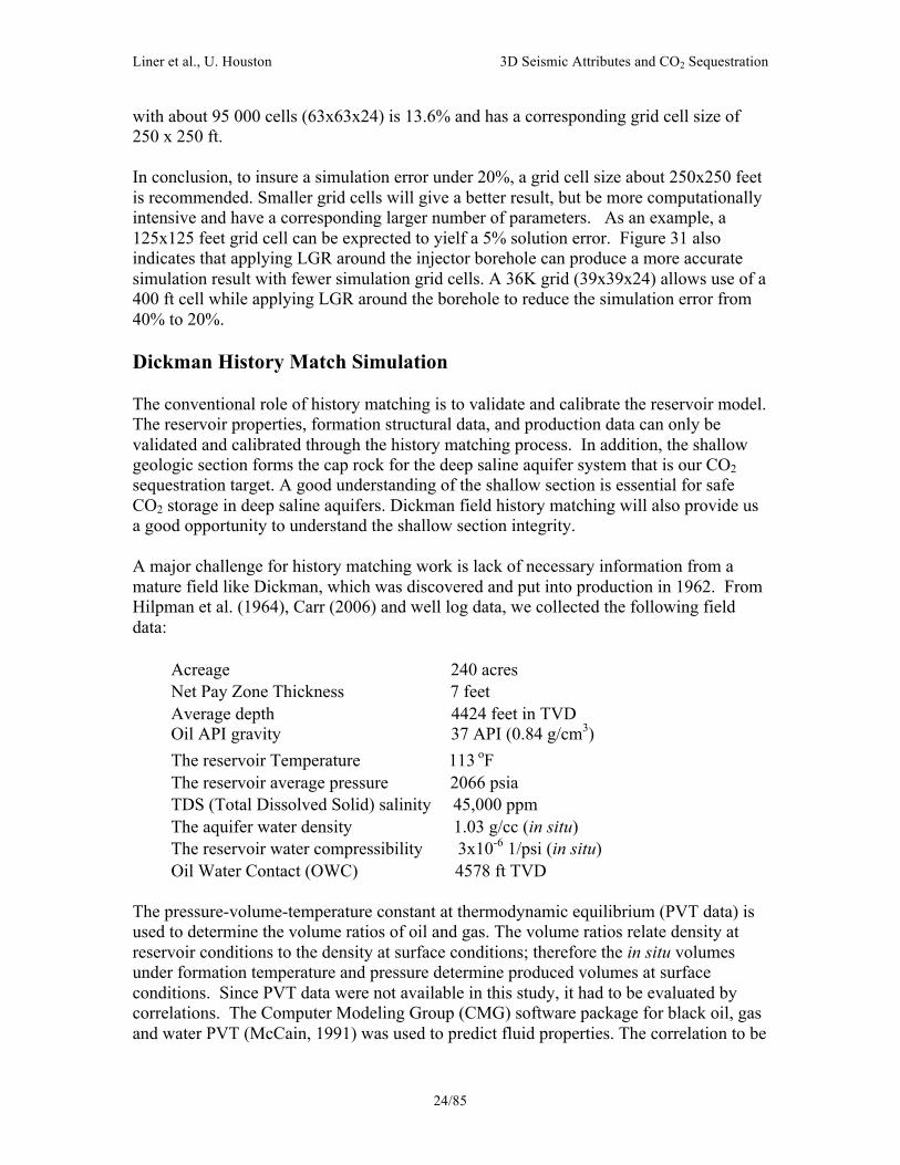
with about 95 000 cells (63x63x24) is 13.6% and has a corresponding grid cell size of 250 x 250 ft. In conclusion, to insure a simulation error under 20%, a grid cell size about 250x250 feet is recommended. Smaller grid cells will give a better result, but be more computationally intensive and have a corresponding larger number of parameters. As an example, a 125x125 feet grid cell can be exprected to yielf a 5% solution error. Figure 31 also indicates that applying LGR around the injector borehole can produce a more accurate simulation result with fewer simulation grid cells. A 36K grid (39x39x24) allows use of a 400 ft cell while applying LGR around the borehole to reduce the simulation error from 40% to 20%. Dickman History Match Simulation The conventional role of history matching is to validate and calibrate the reservoir model. The reservoir properties, formation structural data, and production data can only be validated and calibrated through the history matching process. In addition, the shallow geologic section forms the cap rock for the deep saline aquifer system that is our CO2 sequestration target. A good understanding of the shallow section is essential for safe CO2 storage in deep saline aquifers. Dickman field history matching will also provide us a good opportunity to understand the shallow section integrity. A major challenge for history matching work is lack of necessary information from a mature field like Dickman, which was discovered and put into production in 1962. From Hilpman et al. (1964), Carr (2006) and well log data, we collected the following field data:
Acreage 240 acres Net Pay Zone Thickness 7 feet Average depth 4424 feet in TVD Oil API gravity 37 API (0.84 g/cm3) The reservoir Temperature 113 oF The reservoir average pressure 2066 psia TDS (Total Dissolved Solid) salinity 45,000 ppm The aquifer water density 1.03 g/cc (in situ) The reservoir water compressibility 3x10⁻⁶ 1/psi (in situ) Oil Water Contact (OWC) 4578 ft TVD
The pressure-volume-temperature constant at thermodynamic equilibrium (PVT data) is used to determine the volume ratios of oil and gas. The volume ratios relate density at reservoir conditions to the density at surface conditions; therefore the in situ volumes under formation temperature and pressure determine produced volumes at surface conditions. Since PVT data were not available in this study, it had to be evaluated by correlations. The Computer Modeling Group (CMG) software package for black oil, gas and water PVT (McCain, 1991) was used to predict fluid properties. The correlation to be

Liner et al., U. Houston 3D Seismic Attributes and CO2 Sequestration
25/85
used is determined by an API gravity criterion (Lasater method if API > 15, otherwise Standing method). API value for Dickman field is 37, so Lasater’s correlation was used. In a multiple phase flow system containing oil, gas and water, the relative permeability is a function of phase saturation. Stone correlation formulations were used to generate the relative permeability model for relative permeability of water, oil and water, gas and water, and gas (equations in Appendix B). Figure 32 shows the simulation grid with 15 production wells and one injection well. Table 4 lists production starting date, ending date, and water break through time for all 15 production wells. We have complete oil production data record for all production wells. However, water production records are complete for only five wells: Dickman 1, Humphrey 2, Humphrey 3, Humphrey 4 and Tilley 5. For the remaining production wells, there is either no water production data or only partial data. Dickman 4 is the is used to inject the field waste water back into the reservoir. Because the water injection data record is not available, we assumed that Dickman 4 injected all produced water back to the reservoir. The relative permeability model, well perforation, net pay zone thickness, PVT and capillary pressure model are the reservoir properties being calibrated to match the water and oil production data. These properties have been updated after each of the simulation run. In the final simulation, the original PVT model generated by Lasater’s correlation was used, and generated good matching results. There was no gas or condensate recorded in Dickman field production reports. The compressibility of water is very small, and the effect of gas compressibility on the production volumes of oil and gas is not very significant. A good oil and water history match was obtained on the production wells around the Dickman 4 injector, Dickman 1 being a good example (Figure 33). Dickman 1 is the first production well in the Dickman field and is still produces. Matching the Dickman 1 production is an important step in modeling the entire field. Results also suggest that one main function of the Dickman 4 water injection well is to maintain reservoir pressure. Without it the reservoir pressure would be below 1000 psi at the end of the history matching simulation. The assumption that Dickman 4 injected all produced water back into the reservoir seems to be correct. Well perforation data also plays an important role in history matching. Dickman A1 was reportedly perforated only in the two upper flow model layers (uppermost Mississippian), and the simulated oil production rate is consequently much lower than the real oil production rate (Figure 34a). This caused the simulated total Dickman field production rates to mismatch during the 1993-1998 production period of the Dickman A1 well (Figure 34b). A better history match is obtained by increasing the Dickman A1 bottom hole depth about 9 feet (Figure 35a), so that all four simulation layers could be perforated

Liner et al., U. Houston 3D Seismic Attributes and CO2 Sequestration
26/85
for Dickman A1. This results in an improved result on the total field oil production rate (Figure 35b). Several different capillary pressure models were tested in the simulation to study the influence of the capillary pressure for transition zones. The simulation results indicate that the capillary pressure almost had no influence either on the oil or water production rate, so the capillary pressure effect was removed from the final calculation. Figure 36 shows the reservoir pressure distribution at the end of history matching simulation. Deep Saline Aquifer Storage Scenario Study As shown in Figure 37, the geological model analysis suggested that the aquifer model, based on 3D seismic data and well log data, should consist of the five geological layers:
1. Fort Scott Limestone 2. Cherokee Group 3. Lower Cherokee Sandstone 4. Mississippian Carbonate 5. Lower Mississippian Carbonate
A twenty-four layer simulation model was constructed from the geological model for CO2 sequestration simulation. The relationship of geological layers and simulation layers are as follows:
Simulation Layer Geological Layer Lithology Kv/Kh 1-2 Ford Scott Limestone 0.7 3-5 Cherokee Group Sandstone 0.5 6-7 lower Cherokee Sand Stone 0.5 8-12 Mississippian Carbonate 0.7 13-24 Lower Mississippian Carbonate 0.7
The new and updated permeability and porosity data obtained from well log analysis were used in the simulation model. Based on the core testing results, we assumed the ratio of the vertical permeability vs. horizontal permeability (Kv/Kh) as 0.7 for generalized carbonate and limestone and 0.5 for sandstone. Dickman filed CO2 storage safety is a major consideration. Nghiem et al. (2009), has described the four different trapping mechanisms for injected CO2 (see Figure 28). The mineral trapping mechanism is the safest and permanent solution. The dissolved CO2 in a saline aquifer will decompose into hydrogen cations and bicarbonare ions that in turn react with the minerals in place. These chemical reactions will induce precipitation of carbonate minerals such as calcite, dolomite, and siderite. The process of CO2 precipitation is extremely slow and minimal for the first thousand years after injection.

Liner et al., U. Houston 3D Seismic Attributes and CO2 Sequestration
27/85
Residual gas trapping is a process that traps CO2 as an immobile gas in the porous media, and is considered nearly as permanent/safe as mineral trapping. The classical Land’s residual trapping model is used in the CMG GEM simulator to this process. Figure 38 shows a typical gas relative permeability curve. When the gas (CO2) saturation increases, the gas relative permeability follows the drainage curve (black curve in Figure 38). If at the saturation on the drainage curve, the gas saturation reverses its course and decreases, the gas relative permeability follows the imbibition curve (red curve). The typical value of is 0.3 to 0.4. We assumed in our simulations. CO2 gas is highly soluble in brine. The only safety risk of the dissolved CO2 gas is that the brine and dissolved CO2 may migrate to the surface. According to Carr et al (2008), the underground water migration speed around Dickman field is only about 40 feet per million years, which eliminates the possibility that any dissolved CO2 gas will be migrated to the surface. Thus the solubility trapping is also considered as a safe CO2 trapping mechanism. In CMG GEM simulator, CO2 solubility in brine is calculated by solving the fugacity equation of
where and are the fugacity of CO2 in aqueous phase and gas phase, respectively. The gas fugacity is calculated by using a cubic equation of state (Peng-Roberson equation in the most cases) and the aqueous phase fugacity is calculated by using Henry’s law
where is Henry constant that is a function of temperature, pressure and salinity and is the mole fraction of CO2 in brine. Free CO2 gas trapped in a geological structure represents a real safety threat. This portion of CO2 can migrate to the surface through faults, fractures, a failed cap rock or corroded well pipe. Han et al. (2009) have shown that theoretical well pipe corrosion rates are on the order of 30-60 mm/yr (80 F and 84 Bar), although experiments indicate a much slower corrosion rate on the order of 1-2 mm/yr. A feasible way of improving CO2 storage safety is to accelerate the process of residual gas trapping and solubility trapping. The following trapping indices were defined to give a convenient measurement on the effectiveness of a CO2 injection process:

Liner et al., U. Houston 3D Seismic Attributes and CO2 Sequestration
28/85
Three trapping mechanisms, structural, solubility and gas residual trapping were included in flow simulations. Trapping efficiencies were calculated for two different CO2 injection scenarios: CO2 only injection and CO2 injection with water were calculated. The effectiveness of using a horizontal injection well was also studied. Figure 39 shows the arrangement of a vertical and a horizontal injector for CO2 only injection tests. Both injector wells are perforated in the bottom simulation layer. CO2 injection rate was set to 6.67 × 106 ft3/day or 346 ton/day with the maximum pressure not exceeding 5000 psia. CO2 injection is done for first 25 years, and the injector is shut in thereafter and the fate of CO2 is modeled for the next 225 years. Figure 40 compares the amount CO2 trapped by the different mechanisms for the vertical injection well and horizontal injection well. For CO2 only injection, the total mass of CO2 trapped by solubility and residual gas trapping is about 56% at 250 years. Compared to the vertical well, the horizontal well increases the well perforation length from 25 feet to 2000 feet, but it only increases the total mass of CO2 dissolved in brine water from 13% to 17.4% and TEI from 53% to 56%. Both injector wells are perforated in the bottom simulation layer. CO2 injection rate was set to 6.67 × 106 ft3/day or 346 ton/day, for a total injection of 3.16 MtCO2. Maximum pressure is modeled not to exceed 5000 psia. CO2 injection is done for first 25 years, and the injector is shut in thereafter and the fate of CO2 is modeled for the next 225 years. Figure 41 compares the amount CO2 trapped by the different trapping mechanisms for both vertical and horizontal injection wells. For CO2 only injection, the total mass of CO2 trapped by solubility and residual gas trapping or Trapping Efficiency Index (TEI) is only about 56% at the time of 250 years. Comparing to the vertical well, the horizontal well increases the well perforation length from 25 feet to 2000 feet but it only increases the total mass of CO2 dissolved in brine water or Solubility Trapping Index STI from 13% to 17.4% and TEI from 53% to 56%. The reason of the low CO2 trapping efficiency is the accumulation of a high CO2 concentration around the well bore. An effective way of reducing CO2 concentration around the borehole is to inject water above the perforation during CO2 injection. Figure 42 shows the vertical and horizontal injection well simulation setup for CO2 injection with brine. The bottom perforations are for CO2 injection and the upper perforations are for water injection. CO2 daily injection rate is still 346 ton/day. The maximum water injection rate per day allowed for the vertical well less than 5000 psia is 6500 bbl/day. So we set the water injection rate for both vertical well and horizontal well as 6500 bbl/day. Figure 43 is the comparison of the amount of CO2 trapped by different mechanisms for the entire simulation period. In the case of CO2 injection with water, the horizontal

Liner et al., U. Houston 3D Seismic Attributes and CO2 Sequestration
29/85
injection well can increase CO2 trapping efficiency index (TEI) significantly. A summary of the simulation results for the simulation grid size of 31x33x24 is given in Table 5. Compared to a vertical injection well, a horizontal injection well can increase CO2 trapping efficiency from 58.1% to 94.2%. Another benefit of using a horizontal injection well is that it can reduce the maximum bottom hole pressure significantly. The maximum bottom hole pressure was 2367 psia for the horizontal injection well and the maximum bottom hole pressure was 5000 psia for the vertical injection well.

Liner et al., U. Houston 3D Seismic Attributes and CO2 Sequestration
30/85
References Cited Bahorich, M. and S. Farmer, 1995, 3-D seismic discontinuity for faults and stratigraphic features: The coherence cube: The Leading Edge, 14, no. 10, 1053-1058.
Blakely, R., 2004, Paleogeography and Geologic Evolution of North America, http://jan.ucc.nau.edu/%7Ercb7/nam.html . (date accessed)
Buchanan, R., and T. R. Carr, 2008, Geolgic Sequestration of Carbon Dioxide in Kansas: Kansas Geological Survey, Public Information Circular 27.
Carr, T. R., D. W. Green, and G. P. Willhite, 1999, Improved oil recovery in Mississippian carbonate reservoirs of Kansas: Near term-class 2, Annual Report Submitted to US Department of Energy (DOE), Report no. DOE/BC/14987-10, 168. (date accessed), http://www.kgs.ukans.edu/PRS/publication/OFR99_22/index.html . Carr, T. R., D. F. Merriam, and J. D. Bartley, 2005, Use of relational databases to evaluate regional petroleum accumulation, groundwater flow, and CO2 sequestration in Kansas: AAPG Bulletin, 89, no. 12, 1607–1627. Chopra, S., and K. J. Marfurt, 2005, Seismic attributes - A historical perspective: Geophysics, 70, no 5, 3SO-28SO. Chopra, S., and K. J. Marfurt, 2007, Seismic Attributes for Prospect Identification and Reservoir Characterization (Geophysical Developments No. 11) (Seg Geophysical Developments): Society of Exploration Geophysicists.
Cole, V. B., 1976, Configuration of the top of the Precambrian rocks in Kansas: Kansas Geological Survey, Map M-7, scale 1:500000.
Daniel, F. M., 1963, The Geologic History of Kansas: Kansas Geological Survey Bulletin, 162.
Franseen, E. K., T. R. Carr, W. J. Guy, and D. S Beaty, 1998, Significance of depositional and early diagenetic controls on architecture of a Karstic-Overprinted Mississippian (Osagian) reservoir, Schaben Field, Ness County, Kansas: Presented at the AAPG Annual Meeting.
Franseen, E. K., A. P. Byrnes, J. R. Cansler, D. M. Steinhauff, and T. R. Carr, 2004, The Geology of Kansas—Arbuckle Group: Kansas Geological Survey Current Research in Earth Science, Bulletin 250, (Date accessed), http://www.kgs.ku.edu/Current/2004/franseen/franseen1.html .
Franseen E. K., 2006, Mississippian (Osagean) Shallow-water, mid-latitude siliceous sponge spicule and heterozoan carbonate facies: An example from Kansas with implications for regional controls and distribution of potential reservoir facies: Kansas

Liner et al., U. Houston 3D Seismic Attributes and CO2 Sequestration
31/85
Geological Survey Current Research in Earth Sciences, Bulletin 252, (Date accessed), http://www.kgs.ku.edu/Current/2006/franseen/index.html.
Gerhard, L. C., 2004, A new look at an old petroleum province: Kansas Geological Survey: Kansas Geological Survey Current Research in Earth Sciences, Bulletin 250, (Date accessed) http://www.kgs.ku.edu/Current/ 2004/Gerhard/index.html .
Han, J., J. W. Carey, and J. Zhang, 2009, A coupled water chemistry and corrosion model for high salinity-high CO2 environments with application to wellbore integrity in CO2 sequestration: AGU, Abstract H11J-04. Heinemann, Z.E., C.W. Brand, M. Munka, and Y.M. Chen, 1991, Modeling reservoir geometry with irregular grids: SPERE, 6, no. 2, 225-232. Hilpman, P. L., M.O. Oros, D. L. Beene and E. D. Goebel, 1964, Oil and Gas Development in Kansas during 1963: State Geological Survey of Kansas Bulletin, 172. Izgec, O., B. Demiral, H. Bertin, and S. Akin, 2006, Experimental and Numerical Modeling of Direct Injection of CO2 Into Carbonate Formations: SPE 10809. Kumar, A., R. Ozah, M. Noh, G.A. Pope, G.A., S. Bryant, K. Sepehrnoori, and L.W. Lake, 2005, Reservoir Simulation of CO2 Storage in Deep Saline Aquifers: SPE 89343. Kumar, N. and S. L. Bryant, 2008, Optimizing Injection Intervals in Vertical and Horizontal Wells for CO2 Sequestration: SPE 116661-MS. Marfurt, K. J., 2006, Robust estimates of 3D reflector dip and azimuth: Geophysics, 71, P29
Marshall T. R. and P. H. Heckel, 2006, Sequence stratigraphy and cyclothem correlation of Lower Cherokee Group (Middle Pennsylvanian), Oklahoma to Iowa: South-Central Section: Presented at the 40th Annual Meeting, GSA.
McCabe, P. J., 1991, Geology of coal; environments of deposition, in H. J. Gluskoter, D. D. Rice, and R. B. Talor, eds., Geological Society of America, The Geology of North America, P-2, 469-482.
McCain, W.D. Jr., 1991, Reservoir-Fluid Property Correlations – State of the Art: SPERE, 6, no. 2, 266-272. Merriam D., 1963, Geologic History of Kansas: Kansas Geological Survey Bulletin 162, (date accessed); http://www.kgs.ku.edu/Publications/Bulletins /162/08_patt.html .
Metz, B, O. Davidson, H. de Coninch, M. Loos, and L. Meyer, 2005, Special report on carbon dioxide capture and storage: Cambridge University Press.
Liner et al., U. Houston 3D Seismic Attributes and CO2 Sequestration
32/85
Mo, S., and I. Akervoll, 2006, Modeling Long-Term CO2 Storage in Aquifer With a Black-Oil Reservoir Simulator: SPE 93951.
Moore, R. C., Frye, J. C., and Jewett J. M., 1944, Tabular description of outcropping rocks in Kansas: Geol Survey of Kansas, Bulletin 52, Part 4.
Moore, R.C., 1949, Divisions of the Pennsylvanian System in Kansas: Kansas Geological Survey Bulletin, 83.
Navanit, K., L. Bryant, J. P., Nicot, and C. M. Oldenburg, 2007, Simplified Models for Plume Dynamics, 6th Annual Conference on Carbon Capture and Sequestration - DOE/NETL (Pittsburgh, Pennsylvania)
Newell, K. D., W. L. Watney, D. W. Steeples, R. W. Knapp, and S. W. L. Cheng, 1989, Suitability of high-resolution seismic method to identifying petroleum reservoirs in Kansas-A geological perspective, in D. W. Steeples ed., Geophysics in Kansas: Kansas Geological Survey Bulletin, 226, 9-30.
Nghiem, L., Sammon, P., Grabenstetter, J., Ohkuma, H., 2004, Modeling CO2 Storage in aquifers with a fully-coupled geochemical EOS compositional simulator: SPE 89474.
Nghiem, L., C. Yang, V. Shrivatava, B. Kohse, M. Hassam, D. Chen and C. Card, 2009, Optimization of Residual Gas and Solubility Trapping for CO2 Storage in Saline Aquifer: SPE 119080. Nissen, S. E.,T. R. Carr, and K. J. Marfurt, 2006, Using New 3-D Seismic attributes to identify subtle fracture trends in Mid-Continent Mississippian carbonate reservoirs: Dickman Field, Kansas, Search and Discovery, Article #40189.
Nissen, S. E., K. J. Marfurt, and T. R. Carr, 2004, Identifying Subtle Fracture Trends in the Mississippian Saline Aquifer Unit Using New 3-D Seismic Attributes: Kansas Geological Survey, Open-file Report 2004-56.
Noh, M., L.W. Lake, S.L. Bryant, and A. Araque-Martinez, 2004, Implications of Coupling Fractional Flow and Geochemistry for CO2 Injection in Aquifers: SPE 89474. OuYang. J., 1994, Well Log Interpretations and Reservoir Descriptions: Book Series on Petroleum Exploration in the Tarim Basin, 9, 235–291.
Pierce, W. G., and W. H. Courtier, 1937, Geology and coal resources of the southeastern Kansas coal field: Kansas Geological Survey Bulletin, 24, 1-122.
Pruess, K., J. García, T. Kovscek, C. Oldenburg, J. Rutqvist, C. Steefel, and T.F. Xu, 2002, Intercomparison of numerical simulation codes for geologic disposal of CO2, http://repositories. cdlib.org/lbnl/LBNL-51813. accessed (date accessed).

Liner et al., U. Houston 3D Seismic Attributes and CO2 Sequestration
33/85
Ramaker, B. J., 2006, Influence of Mississippian Karst Topography on Deposition of the Cherokee Group: Ness County, Kansas, http://hdl.handle.net/1808/5544 , (Date accessed). Rijks, E. J. H., and J. C. E. M. Jauffred, 1991, Attribute extraction: an important application in any detailed 3-D interpretation study: The Leading Edge, 10, no. 9, 11-19. Roberts, A., 2001, Curvature attributes and their application to 3D interpretation: First Break, 19.2, 85-99. Sawin, R., E., Franseen, W. Watney, R. West, and G. Ludvigson, 2009, New Stratigraphic Rank for the Carboniferous, Mississippian, and Pennsylvanian in Kansas: Current Research in Earth Sciences, Bulletin 256, Part 1.
Sengul M., 2006, CO2 Sequestration: A Safe transition technology: SPE 98617.
Smythe, J., A. Gersztenkorn, B. Radovich, C-F. Li, and C. Liner , 2004, Gulf of Mexico shelf framework interpretation using a bed-form attribute from spectral imaging: The Leading Edge, 23, 921 Van der Pluijim, B., and S. Marshak, 1997, Earth Structure an Introduction to Structural Geology and Tectonics, McGraw-Hill. Watney, W., W. Guy, and A. Byrnes, 2001, Characterization of Mississippian Osage Chat in South-Central Kansas, AAPG Bulletin, v. 85, no. 1, p. 85-113 Wei, X.R., G.X. Wang, P. Massarotto, and S.D. Golding, 2006, A Case study on the numerical simulation of enhanced coal bed methane recovery: SPE 101135. Xu, T., J. Apps, and K. Pruess, 2002, Reactive geochemical transport simulation to study mineral trapping for CO2 disposal in deep saline arenaceous aquifers: Lawrence Berkeley National Laboratory (Date accessed), http://escholarship.org/uc/item/7hk8s1nx . Zeller, D., 1968, The Stratigraphic Succession in Kansas, 1968: Kansas Geological Survey Bulletin, 189.

Liner et al., U. Houston 3D Seismic Attributes and CO2 Sequestration
34/85
Appendix A: 3D Seismic Processing and Acquisition Parameters Processing Details: (Note that all amplitude data shown in this report is the reprocessed PSTM seismic data migrated by Kurt Marfurt at University of Houston in 2007) Original processing by: Sterling Seismic Services LTD. Date: 12/2001
1. SEGD to internal format conversion Field correlated 2. Geometry and trace edit 3. Gain recovery 4. Surface consistent amplitude analysis and recovery 5. Minimum phase filter application 6. Surface consistent deconvolution Type: spiking operator: 160 ms
Noise: 0.1% 7. Spectral enhancement 20-128Hz 8. Refraction and data correction 9. Green mountain geophysics refraction statics analysis 3D Fathom
Datum: 2600 feet Velocity: VR 9000ft/sec – Vo 3000 ft/sec
10. Iteration 1 velocity/mute analysis and application 11. Surface-consistent automatic statics 200-1000 ms statics gate 12. Iteration 2 velocity/mute analysis and application 13. Surface-consistent automatic statics 150-1050 ms statics gate 14. Final velocity/mute/scale analysis and application 15. CDP-consistent trim statics 4ms max stat 16. Bandpass filter 20/18-128/72 Hz/DM 17. Time variant scaling windows 18. Common depth point stack 19. Spectral enhancement 20-128 Hz 20. Post stack noise suppression FXY Decon 21. Fourier trace interpolation 110 ft xline interval to 82.5 ft 22. 3D FD migration 95% of RMS velocity field 23. Spectral enhancement 20-128 Hz 24. Bandpass Filter 20/24-120-72 Hz/DB 25. Trace balance time variant scaling windows
Acquisition details:

Liner et al., U. Houston 3D Seismic Attributes and CO2 Sequestration
35/85
1. Date Recorded...........................11/2001 2. Crew...........................................Lockhart Geophysical 3. Source Type...............................Vibroseis 4. Sample Rate...............................2 ms 5. Record End Time......................2 seconds 6. Receiver Interval.......................220 ft 7. Receiver Line Interval…...........660 ft 8. Shot Interval..............................65 ft 9. Shot Line Interval......................880 10. Sweep........................................20-128 Hz 12 sec 3DB/OCT 11. Instruments................................GDAPS 12. Format.......................................SEGY 13. Number of Data Channels.........324 MAX
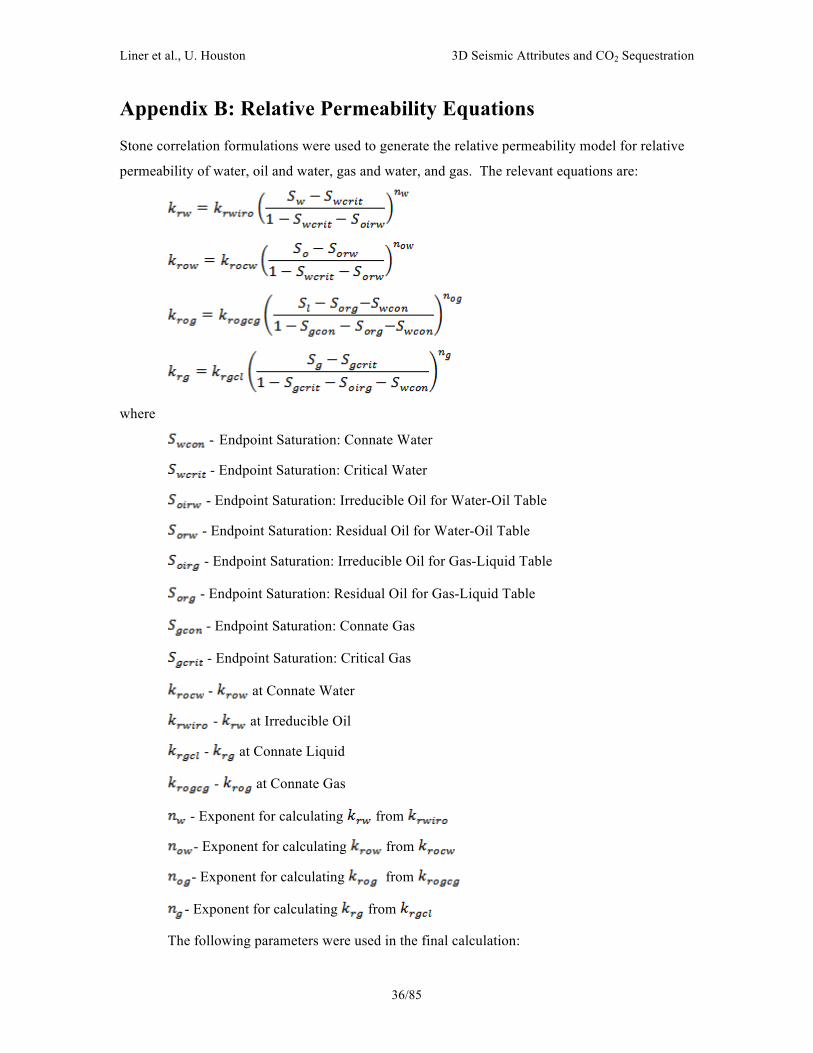
Liner et al., U. Houston 3D Seismic Attributes and CO2 Sequestration
36/85
Appendix B: Relative Permeability Equations Stone correlation formulations were used to generate the relative permeability model for relative
permeability of water, oil and water, gas and water, and gas. The relevant equations are:
where
- Endpoint Saturation: Connate Water
- Endpoint Saturation: Critical Water
- Endpoint Saturation: Irreducible Oil for Water-Oil Table
- Endpoint Saturation: Residual Oil for Water-Oil Table
- Endpoint Saturation: Irreducible Oil for Gas-Liquid Table
- Endpoint Saturation: Residual Oil for Gas-Liquid Table
- Endpoint Saturation: Connate Gas
- Endpoint Saturation: Critical Gas
- at Connate Water
- at Irreducible Oil
- at Connate Liquid
- at Connate Gas
- Exponent for calculating from
- Exponent for calculating from
- Exponent for calculating from
- Exponent for calculating from
The following parameters were used in the final calculation:

Liner et al., U. Houston 3D Seismic Attributes and CO2 Sequestration
37/85
,
,
,
,
,
= 4

Liner et al., U. Houston 3D Seismic Attributes and CO2 Sequestration
38/85
Appendix C: Deep Saline Aquifer Simulation Model Below are a set of detailed figures and a table describing a 31x34x32 deep saline aquifer simulation model for the Dickman project area.
Figure C1: 3D View of simulation model for reservoir fault leaking simulation
Figure C2: 2D center cross section of Figure 1

Liner et al., U. Houston 3D Seismic Attributes and CO2 Sequestration
39/85
Layer Number
Geological Layer Grid Top (TVD,ft) thickness(ft) Porosity
Perm I&J(md)
Perm k(md)
Layer 1 0 300 0.2 30 10 Layer 2 300 300 0.2 30 10 Layer 3 600 300 0.2 30 10 Layer 4 900 300 0.2 30 10 Layer 5 1200 220 0.2 30 10 Layer 6 1320 Map file 0.2 30 10 Layer 7 40 0.2 30 0.01 Layer 8 40 0.2 30 0.01 Layer 9 Fort Scott 0.5xFort Scott FS map FS map 0.7 perm I
Layer 10 Fort Scott 0.5xFort Scott FS map FS map 0.7 perm I Layer 11 Cherokee 1/3xCherokee CH Map CH Map 0.5 perm I Layer 12 Cherokee 1/3xCherokee CH Map CH Map 0.5 perm I Layer 13 Cherokee 1/3xCherokee CH Map CH Map 0.5 perm I
Layer 14 Low
Cherokee 0.5xLCK FS map FS map 0.5 perm I
Layer 15 Low
Cherokee 0.5xLCK FS map FS map 0.5 perm I
Layer 16 Mississippian Unconformity
1xMississippian Unconformity
MissUnconf Map
MissUncon Map 0.7 perm I
Layer 17 Mississippian 0.25xMississippian Miss Map Miss Map 0.7 perm I Layer 18 Mississippian 0.25xMississippian Miss Map Miss Map 0.7 perm I Layer 19 Mississippian 0.25xMississippian Miss Map Miss Map 0.7 perm I Layer 20 Mississippian 0.25xMississippian Miss Map Miss Map 0.7 perm I Layer 21 Osage 0.25xOsage Osage Map Osage Map 0.7 perm I Layer 22 Osage 0.25xOsage Osage Map Osage Map 0.7 perm I Layer 23 Osage 0.25xOsage Osage Map Osage Map 0.7 perm I Layer 24 Osage 0.25xOsage Osage Map Osage Map 0.7 perm I Layer 25 25 Osage Map Osage Map 0.7 perm I Layer 26 25 Osage Map Osage Map 0.7 perm I Layer 27 25 Osage Map Osage Map 0.7 perm I Layer 28 25 Osage Map Osage Map 0.7 perm I Layer 29 25 Osage Map Osage Map 0.7 perm I Layer 30 25 Osage Map Osage Map 0.7 perm I Layer 31 25 Osage Map Osage Map 0.7 perm I Layer 32 25 Osage Map Osage Map 0.7 perm I
Table C1: Layer properties of Dickman deep saline aquifer simulation model

Liner et al., U. Houston 3D Seismic Attributes and CO2 Sequestration
40/85
Figure C3: Layer 7 and 8 are seal layers, shown here in map view with high
permeability fault/fracture.
Figure C4: CO2 Gas saturation at year 250 (injection was simulated for 25 years).

Liner et al., U. Houston 3D Seismic Attributes and CO2 Sequestration
41/85
Tables

Liner et al., U. Houston 3D Seismic Attributes and CO2 Sequestration
42/85

Liner et al., U. Houston 3D Seismic Attributes and CO2 Sequestration
43/85

Liner et al., U. Houston 3D Seismic Attributes and CO2 Sequestration
44/85
Figures

Liner et al., U. Houston 3D Seismic Attributes and CO2 Sequestration
45/85
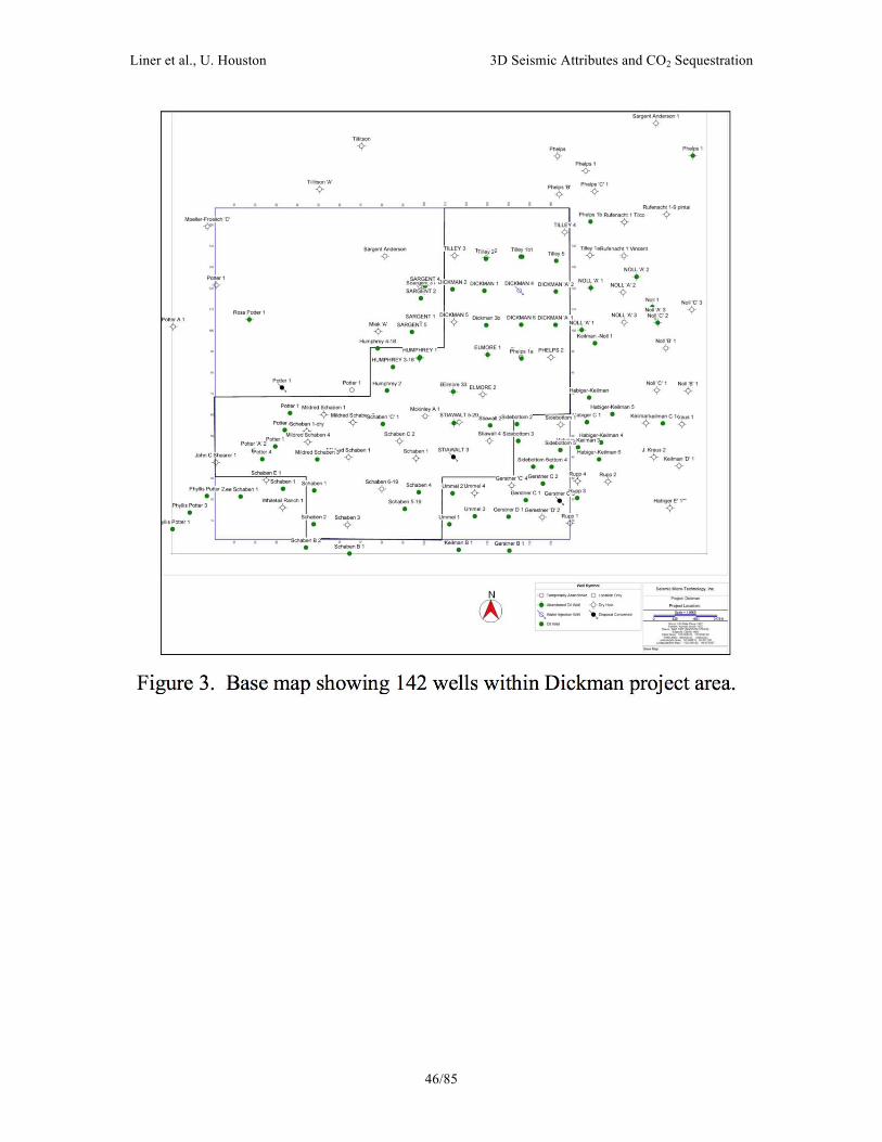
Liner et al., U. Houston 3D Seismic Attributes and CO2 Sequestration
46/85
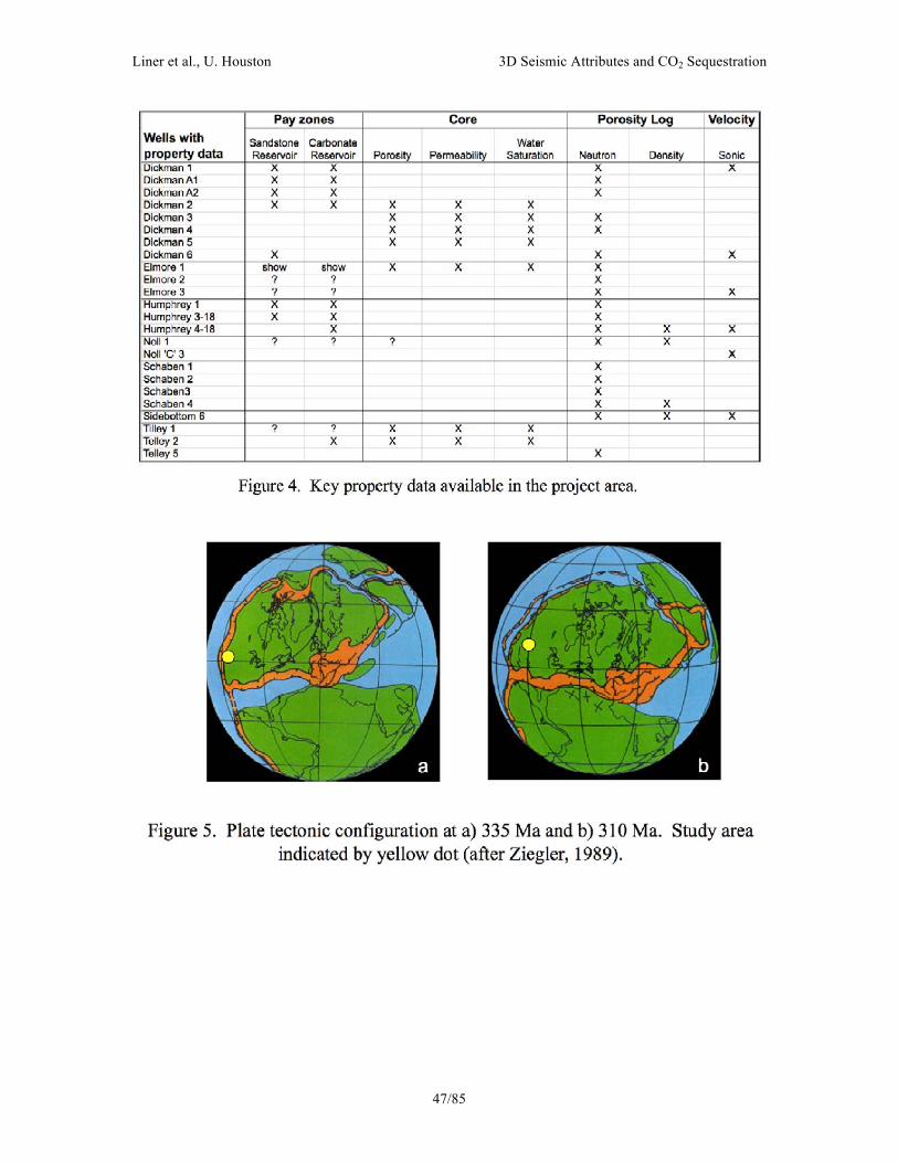
Liner et al., U. Houston 3D Seismic Attributes and CO2 Sequestration
47/85
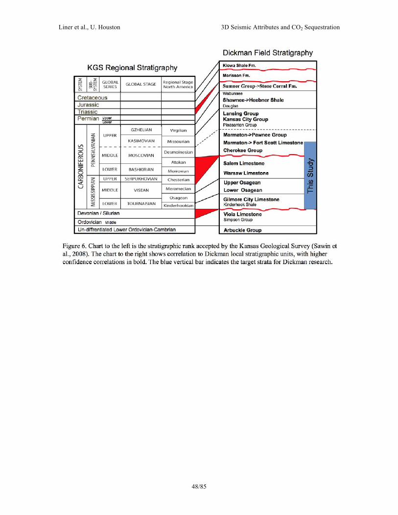
Liner et al., U. Houston 3D Seismic Attributes and CO2 Sequestration
48/85

Liner et al., U. Houston 3D Seismic Attributes and CO2 Sequestration
49/85

Liner et al., U. Houston 3D Seismic Attributes and CO2 Sequestration
50/85
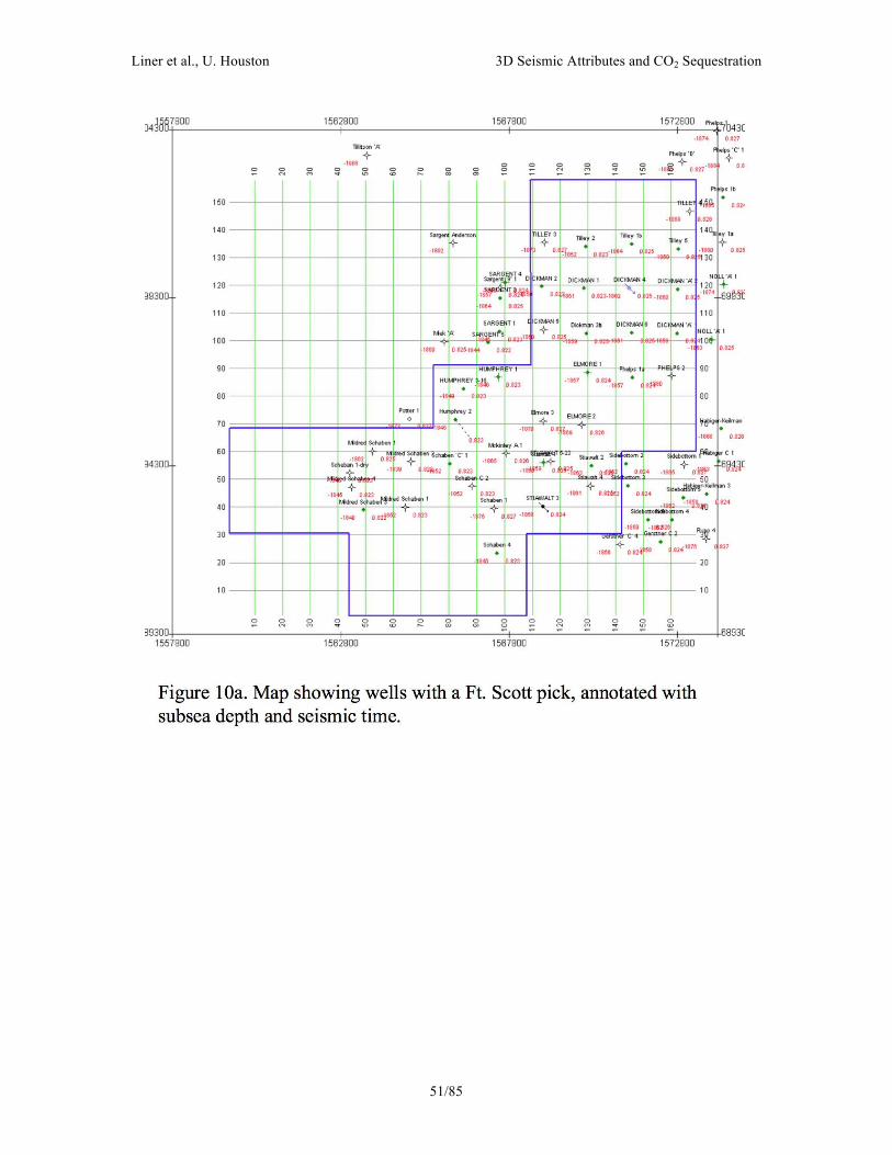
Liner et al., U. Houston 3D Seismic Attributes and CO2 Sequestration
51/85
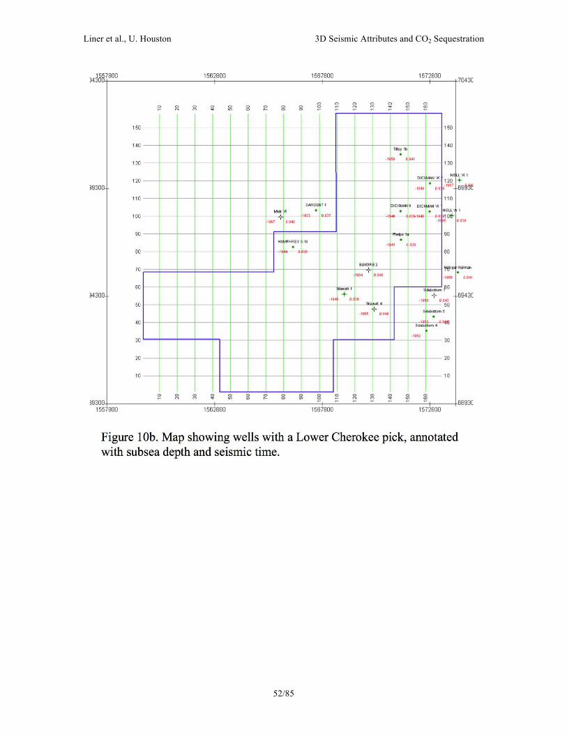
Liner et al., U. Houston 3D Seismic Attributes and CO2 Sequestration
52/85

Liner et al., U. Houston 3D Seismic Attributes and CO2 Sequestration
53/85

Liner et al., U. Houston 3D Seismic Attributes and CO2 Sequestration
54/85

Liner et al., U. Houston 3D Seismic Attributes and CO2 Sequestration
55/85

Liner et al., U. Houston 3D Seismic Attributes and CO2 Sequestration
56/85

Liner et al., U. Houston 3D Seismic Attributes and CO2 Sequestration
57/85

Liner et al., U. Houston 3D Seismic Attributes and CO2 Sequestration
58/85

Liner et al., U. Houston 3D Seismic Attributes and CO2 Sequestration
59/85

Liner et al., U. Houston 3D Seismic Attributes and CO2 Sequestration
60/85

Liner et al., U. Houston 3D Seismic Attributes and CO2 Sequestration
61/85

Liner et al., U. Houston 3D Seismic Attributes and CO2 Sequestration
62/85

Liner et al., U. Houston 3D Seismic Attributes and CO2 Sequestration
63/85

Liner et al., U. Houston 3D Seismic Attributes and CO2 Sequestration
64/85

Liner et al., U. Houston 3D Seismic Attributes and CO2 Sequestration
65/85

Liner et al., U. Houston 3D Seismic Attributes and CO2 Sequestration
66/85

Liner et al., U. Houston 3D Seismic Attributes and CO2 Sequestration
67/85

Liner et al., U. Houston 3D Seismic Attributes and CO2 Sequestration
68/85
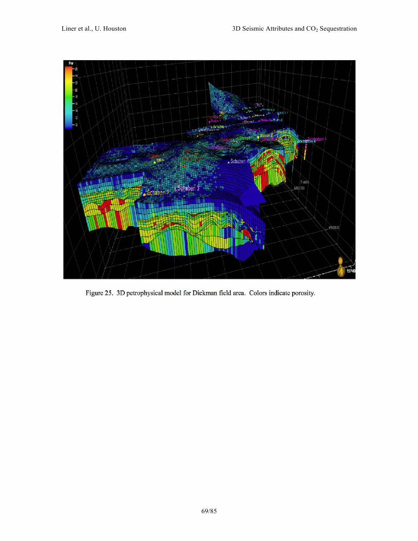
Liner et al., U. Houston 3D Seismic Attributes and CO2 Sequestration
69/85

Liner et al., U. Houston 3D Seismic Attributes and CO2 Sequestration
70/85

Liner et al., U. Houston 3D Seismic Attributes and CO2 Sequestration
71/85

Liner et al., U. Houston 3D Seismic Attributes and CO2 Sequestration
72/85

Liner et al., U. Houston 3D Seismic Attributes and CO2 Sequestration
73/85

Liner et al., U. Houston 3D Seismic Attributes and CO2 Sequestration
74/85

Liner et al., U. Houston 3D Seismic Attributes and CO2 Sequestration
75/85

Liner et al., U. Houston 3D Seismic Attributes and CO2 Sequestration
76/85

Liner et al., U. Houston 3D Seismic Attributes and CO2 Sequestration
77/85

Liner et al., U. Houston 3D Seismic Attributes and CO2 Sequestration
78/85
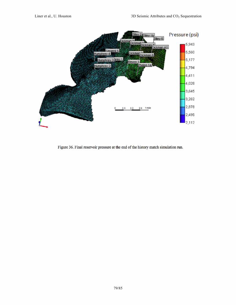
Liner et al., U. Houston 3D Seismic Attributes and CO2 Sequestration
79/85

Liner et al., U. Houston 3D Seismic Attributes and CO2 Sequestration
80/85

Liner et al., U. Houston 3D Seismic Attributes and CO2 Sequestration
81/85

Liner et al., U. Houston 3D Seismic Attributes and CO2 Sequestration
82/85

Liner et al., U. Houston 3D Seismic Attributes and CO2 Sequestration
83/85

Liner et al., U. Houston 3D Seismic Attributes and CO2 Sequestration
84/85

Liner et al., U. Houston 3D Seismic Attributes and CO2 Sequestration
85/85


![Gas Chimmney Detection Thru Seismic Attribute Analysis[1]](https://img.dokumen.tips/doc/110x75/544a573bb1af9f7c4f8b46ee/gas-chimmney-detection-thru-seismic-attribute-analysis1.jpg)