Transportation Research Record 905

reliable classified count data for highway planning and operation.

ACKNOWLEDGMENT

1'~ coop.:-r:ation of TRRL and of the Department of Transport aha the Nottinghamshire County Council as highway authorities is acknowledged. The research is sponsored. by the University of Nottingham Allied Breweries Bequest and is carried out by permission of P.s. Pell, Head of the Department of Civil Engi­neering. Responsibility for the paper and its con­tents, however, remains ours.

REFERENCES

1. Report of the Advisory Committee on Trunk Road Assessment. U.K. Department of Transport, Lon­don, 1977.

2. G. Penrice. Problems of Processing Data Col­lection and Analysis. Presented at Conference on Traffic Data Collection, Institute of Civil Engineers, London, 1978.

3. Traffic Appraisal Manual. U.K. Department of Transport, London, 1981.

4. P. Davies. The Accuracy of Automatic Speed and Length Classification. Department of Civil Engineering, Univ. of Nottingham, England, 1982.

27

5. P. Davies, D.R. Salter, and M. Bettison. Loop Sensors for Vehicle Classification. Traffic Engineering and Control, Vol. 23, No. 2, 1982, pp. 55-59.

6. An Automatic Method to Classify, Count, and Record the Axle Weight of Road Vehicles. U.K. Transport and Road Research Laboratory, Crow­thorne, Berkshire, England, TRRL Leaflet LF 639, 1981.

7 . R.C. Moore, P. Davies, and D.R. Salter. An Automatic Method to Count and Classify Road Vehicles. Presented at International Conference on Road Traffic Signalling, Institution of Elec­trical Engineers, London, 1982.

8. D.R. Salter and P. Davies. The Accuracy of Au­tomatic Vehicle Classification. Presented at 14th Annual Universities Transport Studies Group Conference, Univ. of Bristol, England, 1982.

9. Evaluation of Vehicle Classification Equipment. Maine Department of Transportation, Augusta, 1982.

fublication of this paper sponsored by Committee on Traffic F7ow Theory and Olaracteristics.

Notice: The Transportation Research Board does not endorse products or manufacture rs. Trade and manufacture rs' names appear in this paper because they are considered essential to its object.

Application of Counting Distribution for High-Variance

Urban Traffic Counts

STEPHEN G. RITCHIE

This paper describes an application of the negative binomial counting distribu· tion to high-variance, short-period traffic counts collected on urban arterial roads during peak-period flow conditions. The data were collected at four sites downstream from signalized intersections in metropolitan Melbourne, Australia, during 1977-1978. Alternative parameter estimation techniques are described as well as a simple method for dealing with transient traffic demand patterns. The results of these comparative evaluations suggest that the negative binomial distribution can be applied quite simply to commonly occurring problems that involve high-variance traffic counts and that results are often markedly better than those for other elementary counting distributions such as the Poisson dis· tribution.

The inherent statistical variability of many flow­related attributes of urban transportation systems has important implications for the design, opera­tion, and use of such systems, e.g., in transit ser­vice design (1), traveler mode choice (2,3), and delay at sign-iilized intersections (_!) , to -n;.ne only a few.

Moreover, continued emphasis on transportation systems management policies has increased the need for more accurate and realistic models that are use­ful for urban traffic systems analysis. Such models include basic statistical distributions of traffic characteristics such as vehicle headways, speeds, gap acceptances, and vehicle arrivals at a point, which are routinely used by traffic engineers and analysts in analyzing traffic system performance, designing and improving traffic facilities, and de­veloping traffic simulation models.

This paper is concerned specifically with

traffic-counting distributions, which describe the distribution of vehicle arrivals at a point during a given time interval. Gerlough and Huber (~l have described the elementary traffic-counting distribu­tions, namely, the Poisson distribution, the bino­mial distribution, and the negative binomial (NB) distribution. These statistical distributions have been known to traffic engineers and analysts for some time. However, the NB distribution has not en­joyed the same wide application as the Poisson dis­tribution to traffic problems, despite its apparent superiority under fairly common variable flow-rate conditions where the variance of traffic counts is high.

In this paper an application is described of the NB counting distribution to high-variance traffic counts and more specifically to short-period counts collected on urban arterial roads during peak-period flow conditions. Alternative parameter estimation techniques are described as well as an explicit but simple method for dealing with transient traffic de­mand patterns (i.e., time-varying traffic flow rates). The results of these comparative evalua­tions are presented.

STOCFASTIC NATURE OF URBAN TRAFFIC FLOWS

In an urban arterial road network, one of the major factors that influences the nature of vehicle arriv­als on a link is the presence of upstream signalized intersections. The cyclic interruption to flow pro-

28

duced by signals operating under peak-period traffic conditions tends to result in pulsed flows on the links of an urban network. At points downstream from a signal it can often be observed that during the early portion of a cycle, traffic flow is high and in the form of near-saturated platoons. Later in the cycle the flow is often light: it then con­sists of turning vehicles that have filtered through the upstream intersection and any other vehicles that might have entered the link at minor cross streets.

As Gerlough and Huber (~) have noted, if a traffic-counting interval corresponds to the green portion of the signal cycle or to the complete sig­nal cycle, cyclic effects may be masked. However, if the counting interval is short (e.g., 10 s), there will be periods of high flow and periods of low flow. Thus, combining such short-period counts into one distribution results in a high variance, which produces a variance-to-mean ratio signif i­cantly greater than 1. 0, the value expected if ar­rivals were random and Poisson in nature.

In practice, substantial nonrandomness can also be exhibited by urban traffic counts with counting intervals considerably longer than 10 s. For ex­ample, Newell (.§_) has asserted that typical vari­ance-to-mean ratios of 60-s counts lie between 1. 0 and 1. 5. Williams and Emmerson (ll obtained an av­erage variance-to-mean ratio of 1. 51 in Newcastle, England, and Miller (!!l noted that observations in Birmingham generally produced values between 1.0 and 2. 0 ~ thongh one ~et of data gave ~- ratio of just over 4.0. The data analyzed in this paper indicate that variance-to-mean ratios of 10-s counts taken on multilane urban arterial roads downstream from traf­fic signals can be at least as high as the values mentioned above. Also, invariably, as the variance of the counting distribution increases relative to the mean, the NB distribution provides a better fit to the data than a Poisson distribution.

However, a complication is that during peak peri­ods, traffic demands are typically time dependent, so that significant degrees of nonstationarity are likely to exist in time-series short-period traffic counts collected in the field. In theory, this fac­tor invalidates all elementary counting distribu­tions that are appropriate only for time-stationary processes and suggests that more advanced time­series analyses may be necessary under such condi­tions (9,10). Such analyses, of course, probably exceed ;otonly the experience and time constraints of practicing traffic engineers, but also their com­putational resources and accuracy requirements. In addition, elementary statistical distributions, and particularly the Poisson distribution, have for many years been applied widely by traffic engineers to problems such as the analysis and description of ve­hicle arrivals at a point, the design of turn pock­ets, warrants for traffic signals and pedestrian crossings, as well as accident analysis and simula­tion of traffic flows (11).

It is highly likely tha~ .such distribution• will also prove valuable in the. future, under a range of flow conditions, principally due to their relative simplicity. Accordingly, it is suggested in this paper that when an elementary counting distribution is required for a situation in which the variance of counts is high or is expected to be high, the NB distribution should be given greater consideration than in the past. This distribution will typically be more realistic and will provide a better fit to the data than a Poisson distribution. The remainder of the paper is concerned with empirical estimation and application of the NB distribution.

Transportation Research Record 905

DATA

The data used in this analysis were collected in 1977-1978 at several sites in metropolitan Mel­bourne, Australia, on arterial roads downstream from signalized intersections. Four surveys w~re CC'J"~ ducted, and data were collected manuaD.y by using digital counters. In each survey, a 10-s counting interval was used. This particular interval was chosen because the results of the analyses were to be used in a traffic simulation model, a description of which may be found elsewhere (12). The charac­teristics of each survey site are briefly described below.

The site for surveys 1 and 2 was about 10 km from the Melbourne central business district (CBD) on a major divided (three-lane) circumferential arterial road. Survey durations were 7:30-9:30 a.m. for sur­vey 1 and 3:30-5:15 p.m. for survey 2. The counting station was located approximately 300 m downstream from a signalized intersection with cycle length of about BO s.

Survey 3 was conducted about 19 km from the Mel­bourne CBD on a major divided (three-lane) radial arterial road. The counting station was located ap­proximately 250 m downstream from an intersection with signal cycle length of 100 s. The survey dura­tion was 7:15-10:00 a.m.

Survey 4 was conducted about 16 km from the Mel­bourne CBD on a four-lane undivided radial arterial road. The counting station was located approxi­mately 600 m down.stream from an intersection with signal cycle length of 90 s and about 250 m down­stream from a signalized pedestrian crossing. The survey duration was 7:00-9:15 a.m.

At each site, the adjacent land use was residen­tial. For surveys 1-3, the weather was cool with intermittent showers, whereas for survey 4, the weather was cool and dry.

As expected, time trends in the peak-period flows were evident from 15-min flow profiles for each sur­vey. Analysis of the mean and variance of the 10-s counts from each survey was then undertaken for both individual 15-min intervals and each whole peak pe­riod of counts. These results are shown in Table 1. The high variance-to-mean ratios for these sur­veys, both for 15-min and whole-period counts, are notable, particularly for survey 3 (Table 1), where variance-to-mean ratios of the 10-s counts in some 15-min periods exceeded 5.0, whereas that for the whole period was 4.652. These results are consis­tent with the high degree of nonrandomness, which is to be expected in such urban traffic counts but which has of ten been unaccounted for in previous analyses and studies.

NB DISTRIBUTION

De so r ipt ion

Unlike the single-parameter Poisson distribution, the NB distribution iF specified by two parameters, the mean m and a para1uter k. Both these parameters must be estimated from data or at l&ast from knowl­edge about the mean an1 variance of the data. The main issue, however, concerns the procedure for es­timating the parameter k, as discussed in the next section. It can be shown that the Poisson distribu­tion is obtained as a limiting form of the negative binomial when the parameter k approaches infinity. Furthermore, the NB distribution can be obtained from the Poisson distribution when the Poisson pa-rameter is but varies

constant during each counting interval between intervals with an Erlang (or

Transportation Research Record 905

Table 1. Analysis of 10-s traffic-count resu Its for each study. Time

Survey 1 a 7:30 a.m. 7:45 a.m. 8:00 a.m. 8:15 a.m. 8:30 a.m. 8:45 a.m. 9:00 a.m. 9:15 a.m.

Whole period

Survey 3a 7:15 a.m. 7:30 a.m. 7:45 a.m. 8:00 a.m. 8:15 a.m. 8:30 a.m. 8:45 a.m. 9:00 a.m. 9:15 a.m. 9:30 a.m. 9:45 a.m.

Whole period

Avg Flow (vehicles/IO s)

2.522 2.689 2.856 3.233 3.022 2.822 2.000 1.714 2.615

5.944 5.911 6.156 6.111 6.033 6.333 5.811 4.689 4.166 3.544 3.244 5.268

al 5-min periods starting at tjmes listed below.

Pearson Type III) density function (13). The NB probability P(n) of n arrivals in a given

counting interval can be written in several forms, one of which is

P(n) = (k/(rn + k)] k (rn/(rn + k)JR (n+k- 1)

k-1 (1)

where

n = 0,1,2, ••• , m mean arrival rate, k distribution parameter (k > OJ , and

(n+k-1)

k -1 = (n + k -1)!/n! (k -1)!

Recursion equations have also been derived:

P(o) = [k/(rn + k)] k (2)

P(n) = [(n T k - 1)/n] [rn/(rn + k)] P (n - 1) for n;. 1 (3)

Parameter Estimation

Large-sample methods of parameter estimation for the NB distribution have been summarized by Williamson and Bretherton (14). The principal techniques are the method-of-moments (MM) procedure and the maximum-likelihood (ML) method. In the MM pro­cedure, the first two distribution moments are simply estimated from the sample moments and then used to estimate the parameter k. On the other hand, although the ML method is generally more effi­cient, it is somewhat more complex computationally. It involves finding parameter estimates that maxi­mize the sample-likelihood function, which gives the relative likelihood of observing the sample data as a function of the parameter values (15).

Let f (n) be the observed frequency of n arrivals per counting interval (n= O, 1, 2, ••• ), z be the highest value of n observed, and N be the total num­ber of observations (or counts) • Then

N = L f(n) (4) n=O

Variance/ Mean Ratio

1.142 1.577 1.311 1.675 1.480 1.916 1.494 1.765 1.613

4.009 4.139 4.662 5.415 5.432 5.003 4.946 5.011 2.919 3.596 2.316 4.652

Time

Survey 2a 3:30 p.m. 3:45 p.m. 4:00 p.m. 4:15 p.m. 4:30 p.m. 4:45 p.m. 5:00 p.m.

Whole period

Survey 4a 7:00 a.m. 7:15 a.m. 7:30 a.m. 7:45 a.m. 8:00 a.m. 8:15 a.m. 8:30 a.m. 8:45 a.m. 9:00 a.m.

Whole period

Avg Flow (vehicles/ l 0 s)

1.056 1.622 1.611 1.411 1.767 1.544 1.367 1.483

3.478 5.133 5.256 5.433 4.889 4.189 4.211 4.200 3.600 ·~.488

and the sample mean m is given by

rn = (1/N) L nf(n) n=O

The sample variance v is given by

' ~ v= (1/N(N-l)J j N n~o n

2f(n)- [n~o nf(n)J

2 !

Variance/ Mean Ratio

1.136 1.158 1.321 1.750 1.565 1.574 1.865 1.503

2.728 3.000 2.662 3.412 2.971 3.154 3.130 3.420 2.483 3.084

29

(5)

(6)

By using the MM procedure to estimate the NB pa­rameters, the mean arrival rate m is obtained from Equation 5, whereas the parameter k is obtained from

k=rn/[(v/m)-1] (7)

where m and v are obtained from Equations 5 and 6, respectively. From Equation 7, it is apparent that the variance-to-mean ratio must be greater than 1 to enable the NB distribution to be fitted. Also, as this ratio approaches unity (the value for a Poisson process) , k approaches infinity (also the limiting value for a Poisson process). In addition, it is clear that the MM procedure requires only the sample mean and either the sample variance or the variance­to-mean ratio. The importance of this is that a realistic counting distribution may be specified with only limited sample data, simply on the basis of a mean flow rate and a suitably chosen variance­to-mean ratio. Limited empirical evidence, to be described in the next section, suggests that the variance-to-mean ratio of 10-s traffic counts on urban arterial roads increases nonlinearly with the mean flow rate. The variance-to-mean ratios in Table 1 for surveys 1-4 fall in the range 1.1-5.4. Also, as noted earlier, typical values for 60-s traffic counts have been found to lie between LO and 2.0. These values may provide some guidance in selecting a suitable default variance-to-mean ratio, especially when the variance of counts cannot be calculated directly from sample data in a specific application.

In the ML approach to estimating the distribution parameters, the mean arrival rate m is found, as be­fore, from Equation 5. However, an ML estimator of the parameter k is found from the solution for k

30

(other thank=~> of the equation g(k) = 0:

g(k) = N log (1 + (m/k)] - {ff(!)+ f(2) + ... + f(z)] /k} - { [f(2) + f(3)

+ ... + f(z)] /(k + !)} - ... - [f(z)/(k + z - l)] (8)

The equation g(k) = 0 can be solved directly on many computers and on some programmable calculators by using a standard routine for finding the roots of an equation. Alternatively, an iterative solution pro­cedure such as the Newton-Raphson method (16) may be readily programmed for a microcomputer as well as for some hand calculators. By using the Newton­Raphson method, the value of k for the (j + 1) st iteration is given by

(9)

where k j+l • kj are values of k for the (j + 1) st and jth ite r ations and g(k) is as in Equation B.

g'(k)= [-Nmfk(m + k)] +{ [f(J) + f(2) + ... + f(z)] fk2}

+ {[1'(2)+ 1'(3) + ... + f(i)] /(k + 1)2}

+ . .. + ff'(z)/(k + z - 1)2 1 (10)

In applying Equation 9, a starting value of k (kol can be found by using the MM procedure. How­ever, if initial values of k much greater than the root are taken, spurious results can be obtained. In fact, the ML results reported in this paper were obtained by using Equation 9 with a fixed initial value of ko ~ 1. 0 because, in acme case a, .... v ...... ~.

gence could not be obtained with an MM initial value. To decide when an acceptably accurate estimate of

k has been obtained from Equation 9, a decision rule in the form of a convergence criterion is neces­sary. The criterion used allowed a maximum relative error of 10"' or 0.01 percent. Iterations were terminated when the following inequality was satis­fied:

(11)

Once convergence was achieved, the ML estimate of k was obtained from

(12)

Transient Traffic Demands

In view of the time dependencies exhibited by the peak-period traffic counts for surveys 1-4, a method was proposed that might account more satisfactorily, in a very simple fashion, for the underlying non­stationarity. This involved fitting separate dis­tributions to the 10-s counts in each 15-min inter­val and aggregating the resulting frequencies to form an aggregated whole-period frequency distribu­tion for each survey. The purpose of this procedure was to investigate whether the aggregated distribu­tion of counts would fit the data better while at the same time explicitly recognize the transient nature of the traffic demand pattern for each sur­vey. These results, together with those for the normal method of estimating a single distribution on the whole sample of peak-period counts, are pre­sented in the next section.

RESULTS

A number of comparative analyses were conducted by using each of the four data sets from surveys 1 through 4. These analyses examined several issues, including methods of applying the theoretical count­ing distributions to peak-period counts, parameter­estimation techniques, and goodness-of-fit statis­tics. More specifically, for each of the four

Transportation Research Record 905

surveys the overall goodness of fit of both Poisson and NB distributions to the coll'ected data was de­termined, two methods of applying the Poisson and NB distributions to the peak-period counts were inves­tigated, and in each analysis that involved the NB distribution, two methods of parameter estimation were used, namely, the MM procedure and the ML method. However, before further discussion of these analyses and results, the goodness-of-fit statistics are described.

All goodness-of-fit statistics were based on r pairs of observed and predicted frequencies. For both 15-min and whole-period frequency distribu­tions, the cumulative predicted probability distri­bu.tion (Poisson or NB as appropriate) was used to derive r. The minimum value of r was chosen that satisfied the following:

r-1

L P(r);,. 0.99 (13) r=O

w~ere P(r) is the predicted probability of r vehicle a:rivals in a 10-s counting interval.

Consideration was given to several goodness-of­fit statistics, in particular to Kolmogorov-Smirnov and chi-square statistics. However, the nonpara­metric Kolmogorov-Smirnov test was not employed be­cause the predicted distribution parameters were estimated from the sample (17). Further, use of chi-square statistics would have involved several difficulties. These centered on the statistical requirement for a minimum predicted frequency per cell, which would necessitate combining some ad­jacent frequencies in the tails of distributions and would lead to difficulty or ambiguity in the inter­pretation of chi-square statistics for different models applied to the same data set.

This difficulty or ambiguity may arise not be­cause of the minimum frequency requirement per se, but because different cell structures, different numbers of cells, different numbers of parameters estimated from the observed data and required for the calculation of predicted frequencies, and hence different degrees of freedom can be defined for dif­ferent models. Also, the large sample strictness inherent in these statistics results in very strict tests and a tendency to reject the fit of many models unless they fit the data extremely well (18).

It was therefore judged desirable to use statis­tics that could be readily interpreted and used to compare the goodness of fit of different counting distributions to the same data set. Accordingly, a mean absolute deviation statistic (D) and coeffi­cient of determination (R 2 ) were chosen.

The absolute deviation (d) between any observed and predicted frequency is given by

d = IO(n) - F(n)I (14)

where O(n) is the observed frequency of n arrivals per counting interval and F(n) is the predicted fre­quency of n arrivals per counting interval.

The mean absolute deviation (D) between the ob­served and predicted frequency distribution is then given by

r-1

D = L IO(n) - F(n)l/r (15) n=O

with r defined as before. The main advantage of using absolute differences for D is that if the pre­dicted frequency distribution underestimates some frequencies and overestimates others, positive and negative differences cannot cancel to give a false measure of the overall goodness of fit.

The coefficient of determination was obtained

Transportation Research Record 905 31

Table 2. Fitted counting distributions m• and results for each survey.

Survey Distribution (vehicles/ I 0 s) k Iterations D R2

Poisson 2.615 28.42 0.61 (2.496, 2.734)

NB-MM 2.615 4.266 13.58 0.9! (2.457 ' 2.772) (2.377' 6.156)

NB-ML 2.615 3.439 7 11 .93 0.93 (2.457' 2.772) (2.554, 4.323)

2 Poisson 1.483 26.10 0.79 ( 1.388, 1.578)

NB-MM 1.483 2.949 6.73 0.99 (1.364, 1.601) (1 .823, 4.076)

NB-ML 1.483 2.639 6 5.28 0.99 (1.364, 1.601) (1.741 , 3.538)

3 Poisson 5.268 69.51 0.13 (5.125 , 5.411)

NB-MM 5.268 1.442 14.79 0.79 (4.913, 5.622) (1.232, 1.653)

NB-ML 5.268 1.024 2 8.94 0.94 (4.913, 5.622) (0.908, 1.140)

4 Poisson 4.488 50.84 0.01 ( 4.342, 4.634)

NB-MM 4.488 2.153 13.63 0.76 (4.200, 4.776) (1.778, 2.529)

NB-ML 4.488 1.547 4 9.12 0.89 (4.200, 4.776) (1 .331 , 1.763)

895 percent confidence interv als form and k are shown in pa rentheses and are based on Anscombe's study (!2).

from a linear regression between the predicted and observed frequencies of arrivals for each survey.

As noted earlier, whole-period fits of the count­ing distributions were determined by estimating the distribution parameters from the whole sample of 10-s counts for each survey. The results are shown in Table 2 for the Poisson distribution, NB distri­bution with parameter estimation by the MM procedure (NB-MM), and NB distribution with parameter estima­tion by the ML method (NB-ML). It can be seen that the Poisson fits were inferior to the NB distribu­tion, especially for the higher-flow, higher vari­ance-to-mean ratio surveys, 3 and 4. For these two surveys the Poisson fits were very poor. For all surveys, the NB-ML distributions gave better results than the NB-MM distributionsi the difference was most noticeable for surveys 3 and 4.

For each survey, distribution parameters were then estimated separately for each 15-min interval. The frequency distributions so formed were aggre­gated over each peak period to form aggregated whole-period fits, shown below:

Survey Distribution 0 R' 1 Poisson 25.32 0.66

NB-MM 12.97 0.92 NB-ML 11.88 0,93

2 Poisson 24.39 0.81 NB-MM 7.05 0.98 NB-ML 5.74 0.99

3 Poisson 59.44 0.05 NB-MM 15.18 0.76 NB-ML 9.60 0.92

4 Poisson 47. 77 o.oo NB-MM 13.52 o. 77 NB-ML 9.35 0.89

This approach resulted in some improvement in the Poisson fits, but these were still much worse than either NB fit. In general, there were only marginal changes in the NB fits compared with estimating the NB parameters on the whole sample as in Table 2, al­though surprisingly these changes indicated slight reductions in the goodness of fit of the NB distri-butions.

Because of the marked improvement in statistical goodness of fit of the NB distributions over the Poisson distributions, it was decided to inspect

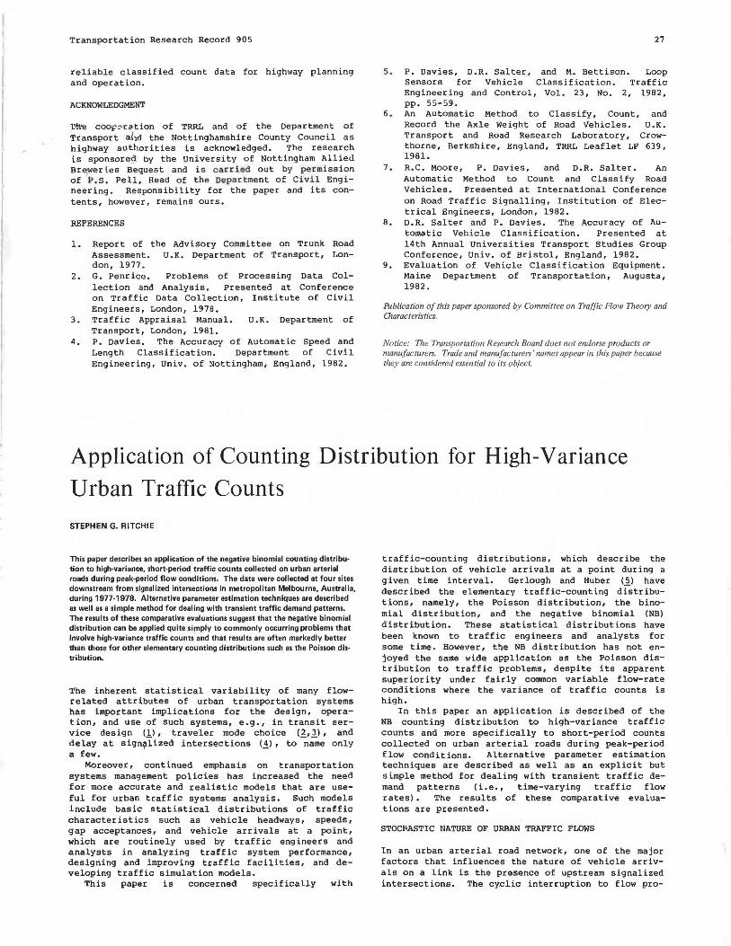
some of the derived NB frequency distributions more closely. Figures 1 through 4 show the observed and aggregated NB-ML frequency distributions for each of the four surveys. At least two features emerge from these figures. First, although the overall fits ap­pear very good, the NB distribution tended to under­estimate slightly the number of intervals with zero arrivals, which were largely caused by the cyclic interruption of the upstream signals. Second, the tails of the fitted distributions were much longer than those of the observed distributions. One rea­son for this latter feature is probably that, like the Poisson distribution, the NB distribution treats vehicles as if they were points. Physical con­straints on the maximum number of vehicles able to pass a point in a given time interval are conse­quently unaccounted for. Such constraints arise, for instance, from finite vehicle lengths, quite apart from any inability or unwillingness on the part of drivers to minimize the gap between their vehicle and the one in front of them. Figures 3 and 4 for surveys 3 and 4, the higher-flow multilane surveys, also show that the NB distribution tended to underestimate the frequency of arrivals in the mid- to higher range of observed arrivals. These arrivals probably consisted of reasonably compact platoons, which are characteristic of flows down­stream from a signal during peak periods. However, the NB distribution also tended to overestimate the frequency of low (but greater than zero) arrival intervals.

Finally, it was observed that the sample vari­ance-to-mean ratios for the 10-s counts in each 15-min interval for each survey tended to vary with the mean flow rate. The following relationship was therefore fitted (with t-statistics in parentheses):

v/m = 1.203 + 0.0956 m2 R2 = 0.81 (7.34) (12.13) (16)

where m and v are as defined previously in Equations 5 and 6 and shown in Table 1 for each survey. The constant in Equation 16, 1.203, is statistically not significantly different from 1.0, the variance-to­mean ratio value for a Poisson process. Equation 16 may thus be interpreted to suggest that as the mean flow rate approaches zero, the limiting counting distribution is a Poisson distribution, whereas the

32

Figure 1. Aggregated frequency distribution: Survey 1.

Frequt>ncy

150

140

130

120

110

100

90

60

70

60

so 40

JO

20

10

0

I

1

I ~ OBSERV ED

0 NB - ML

Figure 2. Aggregated frequency distribution: Survey 2.

Frequency

200

100

180

110

160

150

140

130

120

110 IZl OBSERVED

100 0 NB - ML

90

80

70

60

so 40

30

20

10

departure from a Poisson process increases with the mean flow rate.

Although Equation 16 is based on results for the 15-min intervals in each survey, it was able to pre­dict quite accurately (i.e., well within a 95 per­cent confidence interval) the whole-period variance­to-mean ratio for each survey. Clearly, if further traffic surveys under a broader range of geometric and traffic conditions, and counting intervals, than those in surveys 1-4 confirmed a simple functional relationship such as that in Equation 16, applica­tion of the NB distribution would be further simpli­fied. In that case, the distribution parameters could be estimated (by using the MM procedure) solely from the mean flow rate, as for the Poisson distribution.

CONCLUSIONS

The analysis in this paper suggests that the NB dis­tribution can be applied quite simply to commonly occurring problems involving high-variance traffic counts with results often markedly better than those for other elementary counting distributions, such as the Poisson distribution.

Several methods of fitting counting distributions to time-dependent peak-period counts were investi-

Transportation Research Record 905

Figure 3. Aggregated frequency distribution: Survey 3.

Frequency

180

170

160

150

140

130

120

110

100 ~ OBSERVED

90 D NB - ML

80

70

60

so n 40 I 30

20

10

-""l-'-"l~l-L-"l-L-'1-'-''t-'-"l-L.<f-L.<+'""'4JL..Lf.LX!-'-"lµ..<1-U1-'-''l-'"'+'-'4"- Vehi cl e Arrivals o 1 2 3 • s O 7 B 9 10 n 12 13 •• 1~ 1& ) 17 per 10 sec.

Figure 4. Aggregated frequency distribution: Survey 4.

Frequency

120

110

100

90

BO

70

60

50

40

JO

20

10

0 I

11?:1 OBSERVED

0 N~ - ML

gated, as well as alternative parameter-estimation techniques. From the results, it would appear that unless there is a particular reason to explicitly account for the temporal aspect of peak-period traf­fic demands, as may be the case in a traffic simula­tion study, the simpler method of estimating the NB distribution from the whole sample of peak-period traffic counts is to be preferred. Furthermore, from a practical viewpoint, the somewhat simpler MM parameter-estimation technique may often be pre­ferred to the ML ·method, although the latter yields more efficient parameter estimates. In any case, it is clear that a relatively simple alternative to the Poisson distribution exists, which can yield a much better representation of high-variance, short-period urban traffic counts.

It is hoped that this paper might stimulate re­newed interest in application of the NB counting distribution, pa.rticularly on the part of practi­tioners concerned with urban traffic systems analysis.

ACKNOWLEDGMENT

Much of the research reported in this paper was con­ducted while I was with the Transport Group, Depart­ment of Civil Engineering, Monash University, Aus­tralia. The encouragement and advice of M.A.P. Taylor, Commonwealth Scientific and Industrial Re­search Organization, Australia, in the early stages of this work is gratefully acknowledged.

Transportation Research Record 905

REFERENCES

1. W.C. Jordan and M.A. Turnquist. Zone Schedul­ing of Bus Routes to Improve Service Reliabil­ity. Transportation Science, Vol. 13, No. 3, 1979, pp. 242-268.

2. M.D. Abkowitz. The Impact of Service Reliabil­ity on Work Travel Behavior. Department of Civil Engineering, Massachusetts Institute of Technology, Cambridge, MA, Ph.D. dissertation, 1980.

3. J.N. Prashka. Development of a "Reliability of Travel Modes" Variable for Mode-Choice Mod­els. Transportation Center, Northwestern Univ., Evanston, IL, Ph.D. dissertation, 1977.

4. R.E. Allsop. Delay at a Fixed Time Traffic Signal--!: Theoretical Analysis. Transporta­tion Science, Vol. 6, 1972, pp. 260-285.

5. D.L. Gerlough and M.J. Huber. Traffic Flow Theory. TRB, Special Rept. 165, 1975.

6. G.F. Newell. Approximation Methods for Queues with Application to ' the Fixed-Cycle Traffic Light. SIAM Review, Vol. 7, 1965, pp. 223-237.

7. T.E.H. Williams and J . Emmerson. Traffic Vol­umes, Journey Times and Speeds by Moving­Observer Method. Traffic Engineering and Con­trol, Vol. 3, 1961, pp. 159-162 and 168.

8. A.J. Miller. Settings for Fixed-Cycle Traffic Signals. Proc., Australian Road Research Board Conference, Vol. 2, No. 1, 1964, pp. 342-362.

9. G.E.P. Box and G.M. Jenkins. Time Series Analysis: Forecasting and Control. Holden­Day, New York, 1970.

10. N.W. Polhemus. On the Statistical Analysis of

Non-Homogenous Traffic Streams. Planning and Technology, Vol. 45-54.

33

Transportation 6, 1980, pp.

11. D.L. Gerlough and F.C. Barnes. Poisson and Other Distributions in Traffic. Eno Foundation for Transportation, Saugatuck, CT, 1971.

12. s.G. Ritchie. Bus and Car - Pool Lanes on Ar­terial Roads--A Simulation Study. Proc., Transportation Research Forum, 21st Annual Meeting, Philadelphia, Oct. 1980, Richard B. Cross Co., Oxford, IN, 1980, pp. 280-287.

13. D.J. Buckley. Road Traffic Counting Distribu­tions. Transportation Research, Vol. 1, 1967, pp. 105-116.

14. E. Williamson and M.H. Bretherton. Tables of the Negative Binomial Probability Distribu­tion. Wiley, London, 1963.

15. J.R. Benjamin and C.A. Cornell. Probability, Statistics, and Decision for Civil Engineers. McGraw-Hill, New York, 1970.

16. E. Kreyszig. Advanced Engineering Mathematics, 4th ed. Wiley, New York, 1979.

17 . P.G. Hoel. Introduction to Mathematical Sta­tistics. Wiley, New York, 1966.

18. A. Karlquist and B. Marsjo. Statistical Urban Models. Environment and Planning, Vol. 3, 1971, pp. 83-98.

19. F .J. Anscombe. Sampling Theory of the Negative Binomial and Logarithmic Series Distributions. Biometrika, Vol. 37, 1950.

Publication of this paper sponsored by Committee on Traffic Flow Theory and Owracteristics.

Delay Models of Traffic-Actuated Signal Controls

FENG-BORLIN AND FARROKH MAZOEYASNA

Traffic-actuated signal controls have more control variables for engineers to deal with than a pretimed control. The increased sophistication in their control logic provides greater flexibilities in signal control but also makes the evaluation of their performance more difficult. At the heart of the problem is that traffic de­lays cannot be readily related to the control variables of a traffic-actuated control. This prompts practicing engineers to rely mostly on short-term, subjective field observations for evaluation purposes. To provide an improved capability for evaluating alternative timing settings, delay models are developed in this study for semiactuated and full-actuated controls that employ motion detectors and se­quential phasing. These models are based on a modified version of Webster's formula. The modifications include the use of average cycle length, average green duration, and two coefficients of sensitivity that reflect the degree of sensitivity of delay to a given combination of traffic and control conditions. Average cycle length and average green duration are dependent on the settings of the control variables and the flow pattern at an intersection. They can be estimated by exist­ing methods.

Traffic-actuated controls employ relatively complex logic to regulate traffic flows. This type of logic infuses a much-needed flexibility into signal con­trol, but it also makes the performance evaluation of a traffic-actuated control difficult. A major problem is that traffic delays resulting from such a control cannot be readily related to the settings of the control variables and the flow pattern at an intersection.

Current understanding of traffic delays at a traffic-actuated signal is obtained only through sensitivity analyses with the aid of computer simu-

lation models. Tarnoff and Parsonson <ll have pro­vided a detailed review of the findings of these simulation studies. Computer simulation models, however, have significant limitations.

For one thing, practicing engineers may not be familiar with the nature and the capability of such models. Furthermore, to ensure broad applicabili­ties, simulation models are often difficult to use in terms of data needs, requirements of computer facilities, and the time one has to spend to learn how to use them. As a result, practicing engineers still rely mostly on short-term, subjective field observations in evaluating timing settings.

An alternative to the use of computer simulation is to develop a model in the form of a formula or a set of formulas. Such a model would allow expedient evaluation of a large number of alternatives and would be particularly useful in searching for opti­mal ways of using a signal control. This in turn could encourage practicing engineers to improve the efficiency of existing signal controls.

To partly satisfy this need, this paper presents a set of delay models for semiactuated controls and full-actuated controls that employ motion detec­tors. These delay models are calibrated in terms of simulation data. They are applicable to signal con­trols at individual intersections when single-ring, sequential phasing is used. The traffic flows con-