APPLICATION OF BALANCED ACCEPTANCE SAMPLING TO …

Journal of Landscape Ecology (2017), Vol: 10 / No. 1 aaa

96

APPLICATION OF BALANCED ACCEPTANCE SAMPLING

TO AN INTERTIDAL SURVEY

NAEIMEH ABI1, MOHAMMAD MORADI

2, MOHAMMAD SALEHI

3, JENNIFER BROWN

4,

JASSIM A. AL-KHAYAT5, ELENA MOLTCHANOVA

6

1Dept. of Mathematics and Statistics, University of Canterbury, New Zealand.

2Dept. of Statistics, College of Science, Razi University, Iran.

3Dept. of Mathematics, Statistics and Physics, Qatar University, Qatar.

4Dept. of Mathematics and Statistics, University of Canterbury, New Zealand.

5Dept. of Biological & Environmental Sciences, College of Arts and Science,

Qatar University, Qatar. 6Dept. of Mathematics and Statistics, University of Canterbury, New Zealand.

Received: 28th

March 2017, Accepted: 4th

June 2017

ABSTRACT

In ecological studies, the population of interest is often spread over a large area. In these

studies, obtaining a sample with good spatial coverage is an important feature in the design of

a survey. In most cases adjacent, or neighbouring, units are more similar than units further

apart and the resulting spatial autocorrelation should be taken into account.

Two dimensional systematic sampling (grid-based sampling) is one conventional method

that has been used in environmental studies to achieve spatial coverage of the area.

Balanced Acceptance Sampling (BAS) is a new method for selecting well spread out

sampling units over the study area.

In this paper we will compare the BAS design and two dimensional systematic sampling

for selecting samples (quadrats) from a large area, using a case study of a crab species from

an intertidal marine zone in Qatar.

Keywords: Two dimensional systematic sampling, Balanced acceptance sampling,

Quadrat, Crustacea, Spatial autocorrelation.

INTRODUCTION

In ecological studies, the population of interest can occupy a very large area. Therefore,

obtaining a sample with good spatial coverage is one important aspect to consider in

designing a survey. When adjacent or neighbouring units are more similar than units further

apart, there are advantages in having a sample that is well spread out. By taking into account

the presence of spatial autocorrelation the result should be a representative samples.

There are a number of different sampling strategies that can be used to help in achieving

a well spread out sample (Wang et al., 2012). One of the most common methods for sampling

in two dimensions is systematic sampling. Systematic sampling is used to ensure that the

target population is fully and uniformly represented by the samples collected (Green, 1979).

Although implementing a systematic sampling design is relatively easy, the existence of any

unknown periodic pattern in the population may cause some issues if the interval between

sampling units has the same period (Fattorini et al., 2006; Eberhardt & Thomas, 1991). This

problem is often cited as the biggest disadvantage of systematic sampling.

Abi N., Moradi M., Salehi M., Brown J., Al-Khayat J.A., Moltchanova E.: Application of Balanced Acceptance

aaaaaaaaaaaaaaaaaaaaaaaaaaaaaaaaaaaaaaaaaaaaaaaaaaaaaaaaaaaaaaaaaaaaaaaaaaSampling to an Intertidal Survey

97

During the last decades, a number of sampling methods have been introduced to select

samples that are spread out in a spatial context defined by geographic boundaries, what we

refer to here as “well spread out” samples. Generalized Random Tessellation Stratified

(GRTS) (Stevens Jr & Olsen, 2004), Local Pivotal Methods (LPM1 and LPM2) (Grafström

et al., 2012), Spatially Correlated Poisson Sampling (SCPS) (Grafström, 2012) and Balanced

Acceptance Sampling (BAS) (Robertson et al., 2013) are some of these spatially balanced

sampling methods.

The newest of those, BAS, is one of the simplest computational methods and, although we

do not use this feature in this study, it has the added advantage that it can accommodate more

than two dimensions. BAS is relatively new, and there are limited studies available in the

literature where BAS has been used. L. McDonald et al. (2015) and Keinath & Abernethy

(2016) used BAS to select grid cells in different regions of the United States in order to

ensure the spatial representativeness of the sample in a study of Black-Tailed prairie dogs.

In another study, Howlin & Mitchell (2016) used BAS to select locations in Bighorn Canyon

National Recreation Area in order to monitor bat populations in the area. Here, we

demonstrate the application of BAS to a case study of crustaceans and compare the results of

the implementation with two dimensional systematic sampling method.

The article is organized as follows. A brief overview of the two dimensional systematic

sampling is given in section 2. In section 3 the BAS method is introduced. The crab data set is

described in section 4. In section 5 the results of applying BAS method to the crab data are

reported, practical aspects are discussed in section 6 and, finally in section 7 some

conclusions are drawn.

TWO DIMENSIONAL SYSTEMATIC SAMPLING

Two dimensional systematic sampling has been widely used in environmental studies. Two

dimensional systematic sampling selects the initial sampling unit randomly and uses it as the

origin for a regular pattern, over which the rest of the sampling units are located. Payandeh

(1970) and Tomppo & Heikkinen (1999) have used two dimensional systematic sampling in

forest surveys and found that the relative efficiency of this method depends on the spatial

distribution of the units. For instance, Payandeh (1970) mentioned that the systematic

sampling is more precise than other sampling methods such as stratified or simple random

sampling when applied to original forest areas, while systematic sampling had the least

precision when applied to uniformly spaced populations such as planted production forests.

Mason (1992) found that two dimensional systematic sampling in soil sampling provides

a uniform coverage of the study area.

Two dimensional systematic sampling is as follows: let A be a continuous region,

partitioned into R rows and C columns such that N (N = R×C) non-overlapping rectangle

sites of identical size are formed. In order to select a two dimensional systematic sample of

size n, the N quadrats have to be further stratified into sub-regions each

containing quadrats (D’Orazio, 2003). In the simplest form of two

dimensional systematic sampling, the first sampling unit (first quadrat) is selected at random

from the first sub-region and the others are selected from the remaining sub-regions in the

same relative position as the position of the first quadrat.

Figure 1 illustrates an example of a two dimensional systematic sample. In this example the

goal is to select a sample of size 9. The whole population must be firstly partitioned into

9 (= 3×3) equal sub-regions. One quadrat from each sub-region is selected. In this example,

each sub-region contains 12 (= 4×3) quadrats. The first quadrat is randomly selected from


98

these 12 quadrats in the first sub-region and the other quadrats are chosen from the remaining

sub-regions in the same position as the position of the first selected quadrat. The first

sub-region and the position of the first randomly selected quadrat are shown in Figure 1 in

grey colour and by a circle, respectively.

Fig. 1: An example of a two dimensional systematic sample. The first quadrat, o, is

selected at random from the first sub-region. The first sub-region is shown in grey. The

remaining 8 quadrats are selected from the same relative position from the

8 sub-regions

BALANCED ACCEPTANCE SAMPLING

Balanced acceptance sampling is a new spatially balanced sampling method which selects

samples that are near-evenly distributed (well spread out) over the study area. This method is

based on a special type of quasi-random number sequence, called the Halton sequence

(Halton, 1960). The Halton sequence is constructed by partitioning the unit interval, (0, 1),

with respect to a base ⁄ ⁄ ⁄ and so on, where is a prime number. The

d-dimensional Halton sequence is created by a set of d Halton sequences with pairwise

co-prime bases (Robertson et al., 2013). As an example, the first 10 decimal members of the

2-dimensional Halton sequences are given by the sets

{( ( ) ( ))}

( ) ( ) ( ) ( ) ( )

( ) ( )( ) ( ) ( )

In the first step of implementing the BAS method, it is necessary to specify a hyper box that

encloses the study area (in this paper the study area is restricted in two dimensional space, so

considering just a box is enough). Then, the set of Halton sequences according to the

dimensions of interest would be calculated.

The Halton sequence is deterministic and to introduce some stochasticity in the BAS

method, Robertson et al. (2013) used a random-start Halton sequence. A random-start Halton

sequence is created by skipping some terms in the Halton sequence. For example, the

random-start Halton sequence in two dimensions is achieved after skipping terms in the

first dimension of the Halton sequence and terms in the second dimension of the Halton



99

sequence, where and are two random integers generated from a uniform distribution

on , where is any sufficiently large integer.

The pairs, after skipping some terms, ( ( ) ( )) for k = 1, 2, …,

can be viewed as the spatial coordinates (representing geographic locations) of a point. We

call these pairs Halton points, and they are used to select the BAS sample. If the Halton point

falls in a unit from the sample population the unit is selected. If not, the Halton point will be

discarded and another Halton point is selected, and so on.

The BAS method was first conceived for environmental studies and surveys of natural

resources. In environmental studies, often units in the study area are defined by their

geographical coordinates, and for BAS each geographical axis is considered as a dimension.

Implementing BAS for selecting an equal probability sample of size n in a two dimensional

environmental population could be summarized as follows:

1- Specify a box that encloses the study area.

2- Generate a list of numbers from the Halton sequence in two dimensions.

3- With random starts for the two dimensional Halton sequence, create a sequence of pairs

(Halton points).

4- Take each Halton point in order, and if the observed point falls in a population unit select

the unit for the sample. If not, discard the Halton point and take the next point. Continue

until the desired n sampling units have been selected.

The algorithm to create a BAS sample is surprisingly straightforward and is available

within R (R Core Team, 2016), in the package SDraw (T. McDonald, 2016).

CASE STUDY

We used a data set from a recent study of crabs from Alkhor, in the intertidal zone on the

east coast of Qatar. In a field study in March 2014, a sample of 80 quadrats was selected. The

number of open crab-burrows of the species Nasima dotilliformis was counted in each 1m2

quadrat.

The sample was selected by placing 12 parallel strips at equal distances apart and taking

a systematic sample from each strip, with 6 or 7 quadrats per strip. The latitude and longitude

were recorded for each selected quadrat or sample unit.

We used this information on the quadrat counts and locations to create a synthetic

population of crabs using a Nadaraya-Watson smoother with Gaussian kernel weighting

(Nadaraya, 1964; Watson, 1964 and Nadaraya, 2012). This function can be found in the

package spatstat in R (R Core Team, 2016). The generated counts of Nasima dotilliformis

were a 400×400 matrix, representing the survey population for the study area, which each

entry in the matrix considered the count of crabs in a quadrat. Here we assume each

crab-burrow represents one crab, so that the count of burrows is synonymous with the count

of crabs in our synthetic population.

To compare designs we sampled the population by selecting quadrats with two different

methods: two dimensional systematic sampling and BAS. Simple random sampling (SRS)

method was also considered as a reference method for comparing the results.

To carry out the two dimensional systematic sampling, the population was partitioned into

equal sub-regions according to the desired sample size. For example in the case with


100

a sample size of n=36, the longitude was partitioned into 6 equal intervals, and 36 equal

sub-region would be created. The first quadrat was randomly selected from the first

sub-region. Other quadrats in the remaining sub-regions had the same position as the first

sampling unit within the sub-region.

Spatial coverage

Voronoi polygons can be used as a method for measuring how well spread out a sample is.

This method is based on the distance between elements selected in the sample ( ). The

voronoi polygon , for , includes all population units j satisfying ( ) ( )

for all sampling units , where ( ) indicates the distance between units and .

If ( ) ( ), then unit is included in both and . As a simple example,

consider a population with three units (labeled , and ). The units and are

selected in the sample, and unit is not. Let be the distance between and and

be the distance between and . If then , If then and if

then and , simultaneously. Three different styles of voronoi

polygon which could be created in this example are shown in the Figure 2.

Fig. 2: Three different Voronoi polygons which could be created in a population by

three units. Unit A and B are selected in the sample. (a) D1 < D2 (b) D1 > D2 (c) D1 = D2

Let and denote the number of units in and the sum of inclusion probability in ,

respectively. If unit j is included in polygon, then j is counted as

and its inclusion

probability is divided equally to each of the polygons.

After deriving the voronoi polygons for a given sample, the variance of the voronoi

polygon is calculated by:

( )

∑( )

where indicates the sum of the inclusion probabilities of units in the Voronoi polygon

related to the sampling unit. Stevens Jr & Olsen (2004) used this measure as an indicator

of spatial spread for a given sample where small values of ( ) indicate a very well spread

sample.



101

In our study, for each sample size, the process of selecting samples was repeated 1000

times, and ( ) calculated for each. To compare ( ) among different sampling schemes,

we calculated the average of the ( ) for the 1000 replications:

( ( ))

∑ ( )

,

where ( ) is the Voronoi polygon of the iteration. Small ( ( )) indicates a well

spread out sample, and one with spatial balance.

Parameter estimation

Estimation of population characteristic(s) is usually the final aim of the sampling surveys.

In this study, the total number of crabs in the study area is the parameter of interest. The

Horvitz-Thompson (HT) estimator (Horvitz & Thompson, 1952) can be used for estimating

the total number of crabs in the study area as follow:

∑

,

where is the total number of crabs estimated from the ith

iteration. Also, and

are the number of crabs and the inclusion probability related to the jth

sample quadrat,

respectively.

In this sub-section, we compare the variance of the HT estimator achieved from 1000

simulated samples in three different sampling schemes. The variance of the HT estimator for

1000 simulated sample are estimated by:

( )

∑ ( )

.

Since this study is based on simulation, therefore represents the true total number of

crabs in the study area, 1336781.

We used ( ) to show how precise a sampling method is, with smaller values for

more precise sampling method.

RESULTS

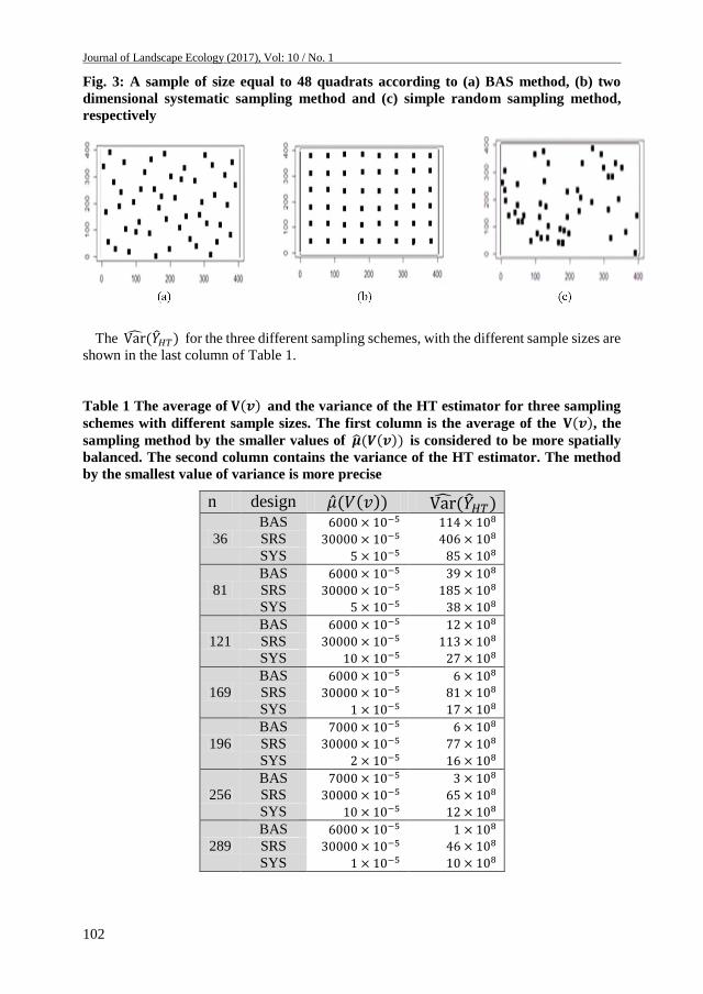
The ( ( )) for three different sampling schemes are shown in first column of Table 1.

The smallest and largest value of ( ( )) is related to the two dimensional systematic

sampling and simple random sampling method, respectively. The very low value of ( ( ))

for systematic sampling can be explained by the survey patterns. For example with a sample

of size n=48, the quadrats (sampling units) which are selected by two dimensional systematic

sampling method have a regular pattern in comparison with two other methods (Figure 3b).

This pattern is obvious in Figure 3b. Figure 3a shows how a sample from BAS and it is more

evenly spread than the sample from SRS (Figure 3c).


102

Fig. 3: A sample of size equal to 48 quadrats according to (a) BAS method, (b) two

dimensional systematic sampling method and (c) simple random sampling method,

respectively

The ( ) for the three different sampling schemes, with the different sample sizes are

shown in the last column of Table 1.

Table 1 The average of ( ) and the variance of the HT estimator for three sampling

schemes with different sample sizes. The first column is the average of the ( ), the

sampling method by the smaller values of ( ( )) is considered to be more spatially

balanced. The second column contains the variance of the HT estimator. The method

by the smallest value of variance is more precise

n design ( ( )) ( )

36

BAS

SRS

SYS

81

BAS

SRS

SYS

121

BAS

SRS

SYS

169

BAS

SRS

SYS

196

BAS

SRS

SYS

256

BAS

SRS

SYS

289

BAS

SRS

SYS



103

Fig. 4: The ( ) achieved by three different sampling methods with different

sample sizes

The trends of the ( ) for the different sampling methods and sample sizes are shown

in Figure 4. With increasing sample size, the variance of all of these methods decreased, and

both BAS and two dimensional systematic sampling had lower variance than simple random

sampling. These two designs had similar estimated variance, with BAS being more precise of

the two dimensional sampling, except with the smaller sample sizes.

FURTHER DISCUSSIONS ABOUT BAS

Of the three designs we used in our study, BAS and two dimensional systematic sampling

were superior to simple random sampling in terms of spatial spread and precision. In addition

to these statistical advantages, there are a number of practical considerations. Encountering

unforeseen factors is a common issue in implementing sampling methods on environmental

fields; therefore designing a flexible method which could adapt to field changes is desirable.

Generally in two dimensional systematic sampling method, the quadrats are selected with

a fixed distance between quadrats and with a regular pattern. Full coverage of the study area

will only be met once the sampling process is completed. In some field situations, completing

the entire sampling process may not be possible, for example if bad weather stops the field

surveys early. In this situation, two dimensional systematic sampling may not have consistent

spread of the quadrats over the study area and there may be gaps where quadrats are not

visited. BAS, on the other hand, is able to cover the study area even when sampling is

stopped early if quadrats are visited in the order they were generated. For more clarity,

assume that because of an extraordinary event we are forced to stop the sampling process at

30 quadrats instead of 48. Fig. 5 shows the quadrats that will be visited by a) BAS and b) two

dimensional systematic sampling if the site ordering is strictly followed.


104

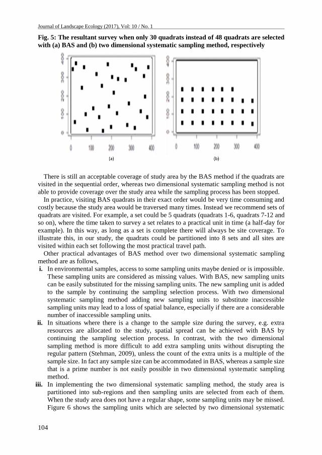
Fig. 5: The resultant survey when only 30 quadrats instead of 48 quadrats are selected

with (a) BAS and (b) two dimensional systematic sampling method, respectively

There is still an acceptable coverage of study area by the BAS method if the quadrats are

visited in the sequential order, whereas two dimensional systematic sampling method is not

able to provide coverage over the study area while the sampling process has been stopped.

In practice, visiting BAS quadrats in their exact order would be very time consuming and

costly because the study area would be traversed many times. Instead we recommend sets of

quadrats are visited. For example, a set could be 5 quadrats (quadrats 1-6, quadrats 7-12 and

so on), where the time taken to survey a set relates to a practical unit in time (a half-day for

example). In this way, as long as a set is complete there will always be site coverage. To

illustrate this, in our study, the quadrats could be partitioned into 8 sets and all sites are

visited within each set following the most practical travel path.

Other practical advantages of BAS method over two dimensional systematic sampling

method are as follows,

i. In environmental samples, access to some sampling units maybe denied or is impossible.

These sampling units are considered as missing values. With BAS, new sampling units

can be easily substituted for the missing sampling units. The new sampling unit is added

to the sample by continuing the sampling selection process. With two dimensional

systematic sampling method adding new sampling units to substitute inaccessible

sampling units may lead to a loss of spatial balance, especially if there are a considerable

number of inaccessible sampling units.

ii. In situations where there is a change to the sample size during the survey, e.g. extra

resources are allocated to the study, spatial spread can be achieved with BAS by

continuing the sampling selection process. In contrast, with the two dimensional

sampling method is more difficult to add extra sampling units without disrupting the

regular pattern (Stehman, 2009), unless the count of the extra units is a multiple of the

sample size. In fact any sample size can be accommodated in BAS, whereas a sample size

that is a prime number is not easily possible in two dimensional systematic sampling

method.

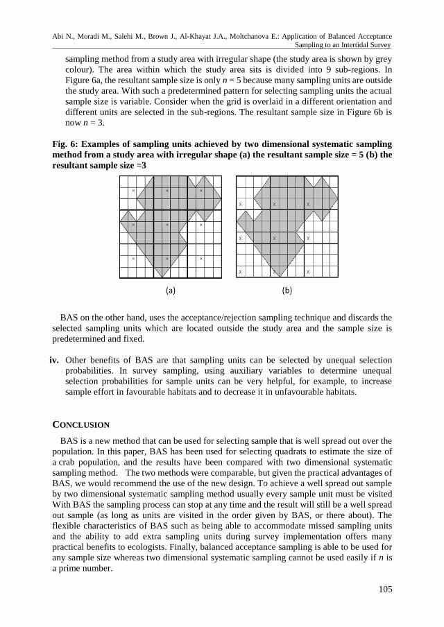
iii. In implementing the two dimensional systematic sampling method, the study area is

partitioned into sub-regions and then sampling units are selected from each of them.

When the study area does not have a regular shape, some sampling units may be missed.

Figure 6 shows the sampling units which are selected by two dimensional systematic



105

sampling method from a study area with irregular shape (the study area is shown by grey

colour). The area within which the study area sits is divided into 9 sub-regions. In

Figure 6a, the resultant sample size is only n = 5 because many sampling units are outside

the study area. With such a predetermined pattern for selecting sampling units the actual

sample size is variable. Consider when the grid is overlaid in a different orientation and

different units are selected in the sub-regions. The resultant sample size in Figure 6b is

now n = 3.

Fig. 6: Examples of sampling units achieved by two dimensional systematic sampling

method from a study area with irregular shape (a) the resultant sample size = 5 (b) the

resultant sample size =3

BAS on the other hand, uses the acceptance/rejection sampling technique and discards the

selected sampling units which are located outside the study area and the sample size is

predetermined and fixed.

iv. Other benefits of BAS are that sampling units can be selected by unequal selection

probabilities. In survey sampling, using auxiliary variables to determine unequal

selection probabilities for sample units can be very helpful, for example, to increase

sample effort in favourable habitats and to decrease it in unfavourable habitats.

CONCLUSION

BAS is a new method that can be used for selecting sample that is well spread out over the

population. In this paper, BAS has been used for selecting quadrats to estimate the size of

a crab population, and the results have been compared with two dimensional systematic

sampling method. The two methods were comparable, but given the practical advantages of

BAS, we would recommend the use of the new design. To achieve a well spread out sample

by two dimensional systematic sampling method usually every sample unit must be visited

With BAS the sampling process can stop at any time and the result will still be a well spread

out sample (as long as units are visited in the order given by BAS, or there about). The

flexible characteristics of BAS such as being able to accommodate missed sampling units

and the ability to add extra sampling units during survey implementation offers many

practical benefits to ecologists. Finally, balanced acceptance sampling is able to be used for

any sample size whereas two dimensional systematic sampling cannot be used easily if n is

a prime number.


106

REFERENCE

D’Orazio, M. (2003). Estimating the variance of the sample mean in two-dimensional

systematic sampling. Journal of Agricultural, Biological, and Environmental Statistics, 8(3),

280-295.

Eberhardt, L., & Thomas, J. (1991). Designing environmental field studies. Ecological

Monographs, 61(1), 53-73.

Fattorini, L., Marcheselli, M., & Pisani, C. (2006). A three-phase sampling strategy for

large-scale multiresource forest inventories. Journal of Agricultural, Biological, and

Environmental Statistics, 11(3), 296-316.

Grafström, A. (2012). Spatially correlated Poisson sampling. Journal of Statistical Planning

and Inference, 142(1), 139-147.

Grafström, A., Lundström, N. L., & Schelin, L. (2012). Spatially balanced sampling through

the pivotal method. Biometrics, 68(2), 514-520.

Green, R. H. (1979). Sampling design and statistical methods for environmental biologists:

John Wiley & Sons.

Halton, J. H. (1960). On the efficiency of certain quasi-random sequences of points in

evaluating multi-dimensional integrals. Numerische Mathematik, 2(1), 84-90.

Horvitz, D. G., & Thompson, D. J. (1952). A generalization of sampling without replacement

from a finite universe. Journal of the American statistical Association, 47(260), 663-685.

Howlin, S., & Mitchell, J. (2016). Monitoring Black-Tailed Prairie Dogs in Colorado with

the 2015 NAIP Imagery.

Keinath, D. A., & Abernethy, I. (2016). Bat population monitoring of bighorn canyon

national recreation area: 2015 progress report.

Mason, B. J. (1992). Preparation of soil sampling protocols: sampling techniques and

strategies. Retrieved from

McDonald, L., Mitchell, J., Howlin, S., & Goodman, C. (2015). Range-Wide Monitoring of

Black-Tailed Prairie Dogs in the United States: Pilot Study.

McDonald, T. (2016). SDraw: Spatially Balanced Sample Draws for Spatial Objects. R

package version 2.1.3. https://CRAN.R-project.org/package=SDraw.

Nadaraya, E. (1964). On estimating regression. Theory of Probability & Its Applications,

9(1), 141-142.

Nadaraya, E. (2012). Nonparametric estimation of probability densities and regression

curves (Vol. 20): Springer Science & Business Media.

Payandeh, B. (1970). Relative efficiency of two-dimensional systematic sampling. Forest

science, 16(3), 271-276.

R Core Team, (2016, September). A language and environment for statistical computing. R

Foundation for Statistical Computing, Vienna, Austria. 2015. Retrieved September 5, 2016,

from URL http. www.R-project.org.

Robertson, B., Brown, J., McDonald, T., & Jaksons, P. (2013). BAS: Balanced acceptance

sampling of natural resources. Biometrics, 69(3), 776-784.

Stehman, S. V. (2009). Sampling designs for accuracy assessment of land cover.

International Journal of Remote Sensing, 30(20), 5243-5272.

Stevens Jr, D. L., & Olsen, A. R. (2004). Spatially balanced sampling of natural resources.

Journal of the American statistical Association, 99(465), 262-278.



107

Tomppo, E., & Heikkinen, J. (1999). National forest inventory of Finland—past, present and

future. Statistics, registries and research-experiences from Finland, 89-108.

Wang, J.-F., Stein, A., Gao, B.-B., & Ge, Y. (2012). A review of spatial sampling. Spatial

Statistics, 2, 1-14.

Watson, G. S. (1964). Smooth regression analysis. Sankhyā: The Indian Journal of Statistics,

Series A, 359-372.

Documents

APPLICATION OF BALANCED ACCEPTANCE SAMPLING TO …