Embed Size (px)
Citation preview
APPLICATION OF AN INVERSE-HYSTERESIS ITERATIVE CONTROLALGORITHM FOR AFM FABRICATION
A thesis submitted in partial fulfillment of the requirements for the degree ofMaster of Science in Mechanical and Nuclear Engineering
at Virginia Commonwealth University
by
SETH C. ASHLEY
B. S., Electrical Engineering, Virginia Commonwealth University, 2006
Major Director:
Kam K. Leang, Ph.D.Assistant Professor, Mechanical Engineering, University of Nevada, Reno
Virginia Commonwealth University
Richmond, Virginia
December 2010

c© Copyright
Seth C. Ashley
All Rights Reserved
December, 2010

Acknowledgment
During the course of this study, I have had the pleasure of working with many
people whose contribution to this thesis deserves special mention. It is a pleasure to
convey my gratitude to them in my humble acknowledgment.
First, I wish to convey my gratitude to a power greater than myself for blessing
my life and for all of the people who have graced it.
I would like to express my sincere appreciation to my advisor, Prof. Kam
Leang, for the continued, tireless demand for my best work. It was his excitement
and energy that motivated the joy I found in precision controls. He has inspired and
enhanced my growth as a student, a researcher, a scientist, and an engineer. I am
indebted to him more than he knows.
I extend my gratitude to the members of my committee, Prof. Karla Mossi,
Prof. Yuichi Motai, and Prof. John Speich, for their guidance and for ushering me
through the final chapters of my studies. I am also very grateful to Prof. Gary
Atkinson for the advice and guidance throughout my academic career, and for helping
to foster my appreciation of the micro-sized world.
Sincere gratitude is also extended to my parents, Garold and Petrine, and my
sister, Jessica, for supporting me financially, emotionally, and spiritually throughout
my academic career. I thank all three of them for not only making me want to, but
for showing me how to step away from the wall and dance!
Finally, this work would not be possible without the unwavering support of my
wife, Sharon. Her love, understanding, and patience are unmeasurable and truly ap-
preciated. Sharon’s dedication, faith, loyalty, conscientiousness, and positive attitude
have made me a better man. I hope this work honors her love and her contribution.
iii

Dedication
To my wife and son.
I hope this work makes you proud.
iv

Table of Contents
List of Figures vii
List of Tables ix
Abstract x
Chapter 1 Introduction 1
1.1 Thesis Goal and Objective . . . . . . . . . . . . . . . . . . . . . . . . 1
1.2 The Need for Precision Positioning . . . . . . . . . . . . . . . . . . . 2
1.3 Challenges in Precision Positioning of Piezoactuators . . . . . . . . . 3
1.4 Piezoactuator Control Approaches . . . . . . . . . . . . . . . . . . . . 6
1.5 Proposed Approach . . . . . . . . . . . . . . . . . . . . . . . . . . . . 9
1.6 Thesis Outline . . . . . . . . . . . . . . . . . . . . . . . . . . . . . . . 10
Chapter 2 The Atomic Force Microscope 11
2.1 History of Microscopy . . . . . . . . . . . . . . . . . . . . . . . . . . 11
2.2 Atomic Force Microscopy . . . . . . . . . . . . . . . . . . . . . . . . . 14
2.3 Hysteresis Modeling and Compensation . . . . . . . . . . . . . . . . . 24
2.4 Summary . . . . . . . . . . . . . . . . . . . . . . . . . . . . . . . . . 33
Chapter 3 Iterative Control for Hysteresis Compensation 35
3.1 Motivation . . . . . . . . . . . . . . . . . . . . . . . . . . . . . . . . . 35
3.2 Review of Iterative Control Methods . . . . . . . . . . . . . . . . . . 38
3.3 Iterative Compensation of Hysteresis . . . . . . . . . . . . . . . . . . 45
3.4 Inverse-Hysteresis Iterative Control . . . . . . . . . . . . . . . . . . . 49
3.5 Summary . . . . . . . . . . . . . . . . . . . . . . . . . . . . . . . . . 52
v

Chapter 4 Experimental System and Implementation 54
4.1 Experimental System . . . . . . . . . . . . . . . . . . . . . . . . . . . 55
4.2 Iteration Process . . . . . . . . . . . . . . . . . . . . . . . . . . . . . 62
4.3 Summary . . . . . . . . . . . . . . . . . . . . . . . . . . . . . . . . . 68
Chapter 5 Experimental Results 70
5.1 Hysteresis Without Compensation . . . . . . . . . . . . . . . . . . . . 71
5.2 Hysteresis Modeling . . . . . . . . . . . . . . . . . . . . . . . . . . . . 71
5.3 Calculating Iteration Gains α and ρ . . . . . . . . . . . . . . . . . . . 73
5.4 Application of Iterative Control . . . . . . . . . . . . . . . . . . . . . 76
5.5 Comparative Results . . . . . . . . . . . . . . . . . . . . . . . . . . . 81
Chapter 6 Conclusions 83
Chapter 7 Future Work 86
List of References 88
Appendix A MATLAB and C Program Examples 104
A.1 Inverse-Hysteresis ICA C Code . . . . . . . . . . . . . . . . . . . . . . 104
A.2 MATLAB Code . . . . . . . . . . . . . . . . . . . . . . . . . . . . . . 114
Vita 119
vi

List of Figures
1.1 The nonlinear input versus output curve demonstrates hysteresis. . . 5
2.1 The main components of a scanning tunneling microscope. . . . . . . 13
2.2 The raster atomic force microscope (AFM) imaging trajectory. . . . . 15
2.3 The fundamental operation of the AFM. . . . . . . . . . . . . . . . . 15
2.4 The main components of an AFM system. . . . . . . . . . . . . . . . 16
2.5 A quartered photo-detector can detect the torsional and vertical de-
flection of the cantilever. . . . . . . . . . . . . . . . . . . . . . . . . 21
2.6 The tube piezoactuator with properly placed electrodes allows displace-
ment in all three directions. . . . . . . . . . . . . . . . . . . . . . . . 23
2.7 The hysteretic air conditioning system. . . . . . . . . . . . . . . . . . 24
2.8 Hysteresis as demonstrated by an applied voltage and the measured
displacement. . . . . . . . . . . . . . . . . . . . . . . . . . . . . . . . 27
3.1 A block diagram description of iterative control. . . . . . . . . . . . 39
4.1 A schematic of the main components of the experimental AFM system. 56
4.2 A photograph of the 5500 AFM courtesy of Agilent Technologies, Inc. 56
4.3 A block diagram of the experimental AFM system. . . . . . . . . . . 57
4.4 A scanning electron microscopy image of the underside of the AFM
probe used in this study courtesy of NANOSENSORSTM. . . . . . . . 58
4.5 Frequency response of the piezoactuator of the AFM system. . . . . . 60
4.6 The desired trajectory in (a) the x- and y- axes and (b) a top view of
the desired circular fabrication trajectory. . . . . . . . . . . . . . . . 61
vii

4.7 The desired (a) x- and (b) y-axis trajectories partitioned into mono-
tonic sections. . . . . . . . . . . . . . . . . . . . . . . . . . . . . . . . 64
4.8 Input versus output curve used to calculate the inverse hysteresis of
the y-axis. . . . . . . . . . . . . . . . . . . . . . . . . . . . . . . . . . 65
4.9 The complementary inverse-hysteresis data is interpolated using the
two closest data-points to the output value of interest. . . . . . . . . 66
4.10 The signal input before each iteration to reset the past-input memory
of the piezoactuator to the same initial condition. . . . . . . . . . . . 67
5.1 The open-loop, uncompensated performance of the piezoactuator. . . 72
5.2 The general desired trajectories with monotonic sections of interest xd
and yd. . . . . . . . . . . . . . . . . . . . . . . . . . . . . . . . . . . . 77
5.3 Results of proportional iterative control applied to the x-axis. . . . . 78
5.4 Experimental results of proportional iterative control as applied to the
y-axis. . . . . . . . . . . . . . . . . . . . . . . . . . . . . . . . . . . . 79
5.5 The inverse-hysteresis iterative control algorithm (ICA) as applied to
the x- and y- axes. . . . . . . . . . . . . . . . . . . . . . . . . . . . . 80
7.1 Cascade model of a piezoactuator. . . . . . . . . . . . . . . . . . . . . 86
A.1 The inputs over 55 iterations of the inverse-hysteresis ICA as developed
by the custom MATLAB code. . . . . . . . . . . . . . . . . . . . . . . 114
viii

List of Tables
5.1 Polynomial models of the x- and y-axis trajectories. . . . . . . . . . . 73
5.2 The constants ξ1, ξ2, M , and α as calculated for the x-axis trajectory. 76
5.3 The constants ξ1, ξ2, M , and α as calculated for the y-axis trajectory. 76
5.4 Comparison of number of iterations to achieve various levels of maxi-
mum error for the proportional P-type and inverse-hysteresis H−1 it-
erative control algorithms. . . . . . . . . . . . . . . . . . . . . . . . . 81
ix

Abstract
APPLICATION OF AN INVERSE-HYSTERESIS ITERATIVE CONTROLALGORITHM FOR AFM FABRICATION
By Seth C. Ashley, M. S.
A thesis submitted in partial fulfillment of the requirements for the degree ofMaster of Science in Mechanical and Nuclear Engineering
at Virginia Commonwealth University.
Virginia Commonwealth University, 2010
Major Director:Kam K. Leang, Ph.D.
Assistant Professor, Mechanical Engineering, University of Nevada, Reno
An iterative control algorithm (ICA) which uses an approximate inverse-hysteresis
model is implemented to compensate for hysteresis to precisely fabricate features on
a soft polymer substrate using an atomic force microscope (AFM). The AFM is an
important instrument in micro/nanotechnology because of its ability to interrogate,
manipulate, and fabricate objects at the micro/nanoscale. The AFM uses a piezo-
electric actuator to position an AFM-probe tip relative to the sample surface in three
dimensions. In particular, precision lateral control of the AFM-probe tip relative
to the sample surface is needed to ensure high-performance operation of the AFM.
However, precision lateral positioning of the AFM-probe tip is challenging due to
significant positioning error caused by hysteresis effect. An ICA which incorporates
an approximate inverse of the hysteresis behavior is proposed to compensate for the
hysteresis-caused positioning error. The approach is applied to fabricate a feature us-
ing the AFM on a polycarbonate surface, and it is demonstrated that the maximum
tracking error can be reduced to 0.225% of the displacement range, underscoring the
benefits of the control method.
xi

Chapter 1
Introduction
1.1 Thesis Goal and Objective
The goal of this thesis is to reduce the number of iterations required by a feedforward
iterative controller to minimize the hysteresis-caused positioning error in piezo-based
atomic force microscopy (AFM) (Binnig et al., 1986), a type of scanning probe mi-
croscope (SPM). The objective to achieve this goal is to apply an iterative control
algorithm where the input-update law uses an approximate hysteresis-inverse model
to increase the convergence rate. The improved performance offered by the new con-
trol approach addresses the need for precision control of SPMs to advance the state-
of-the-art of many fields of nanotechnology, including micro- and nano-fabrication
applications (Snow et al., 1997).
The AFM uses a small micro-cantilever with a sharp tip (similar to a phono-
graph arm and stylus) to “feel” the surface of the sample. The cantilever tip is often
positioned over the sample surface (in the three-dimensions, x, y, and z) using a
piezoactuator in applications that include imaging DNA (Allison et al., 1996), study-
ing the nanomechanical properties of human hair (Bhushan and Chen, 2006), and
exploring the nanostructure of food (Shimoni, 2008). Due to the hysteresis effect in
the piezoactuator, significant positioning error exists which limits the performance
1

of existing piezo-based AFM systems, and SPM systems in general (Clayton et al.,
2009). This work experimentally validates an approach which takes advantage of
an inverse-hysteresis model for iterative control. Specifically, the contribution is the
application of an input-update law which incorporates an approximate inverse of the
hysteresis effect measured experimentally for improved tracking performance com-
pared to previous work.
Many different methods have been used to compensate for hysteresis in piezo-
based scanning probe systems, including feedback control (Devasia et al., 2007), feed-
forward control (Fleming and Wills, 2009; Leang et al., 2009b), and iterative control
(Clayton et al., 2009; Wu and Zou, 2006). In particular, an iterative control algorithm
was developed for hysteretic systems and applied to AFM imaging (Leang and Deva-
sia, 2006). Convergence of the algorithm was proven and its performance quantified;
however, the structure of the input-update law was chosen conservatively. This work
improves upon the previously developed iterative control algorithm by considering an
approximate inverse-hysteresis model in the input-update law.
1.2 The Need for Precision Positioning
Precision positioning in SPM is critical in many micro- and nano-scale applications.
For example, an AFM has been used to precisely place the nanogap electrode in a
nanogap single electron transistor (Moriya et al., 2010); a scanning probe microscope
has been used to indent a semiconductor surface to facilitate the growth of quantum
2

dots (Murakami et al., 2001; Taylor et al., 2005); and the mechanical properties of
quantum dots have been investigated using a piezoactuator-driven nano-indenting
tool (McCumiskey, 2009). Quantum dots are made more efficient by growing them
closer together – on the order of tens of nanometers in pitch (Krauss, 2005), and the
properties (for example, luminescent intensity) of quantum dots have been shown to
be greatly impacted by a 4 nm deviation in size and/or spacing (Leonard et al., 1993).
Thus, nano-precision positioning control of the SPM probe is required to achieve the
spacing necessary for the fabrication of the most efficient quantum dots with desired
properties.
Likewise, there is growing interest in AFM fabrication techniques (Wiesendan-
ger, 1994), and the AFM is a valuable tool in micro- and nano-fabrication of organic
and inorganic structures (Snow et al., 1997). As the applications for AFM fabrication
increase in number and the size of fabricated components become smaller and smaller,
the necessity for precise control of the piezoactuator becomes important.
1.3 Challenges in Precision Positioning of Piezoactuators
Most scanning probe microscopy techniques use a piezoactuator for a number of good
reasons – they have high mechanical resonance (i.e., stiff), low power consumption,
they are compact, have fast response times (acceleration rates of 98 km/s2 have been
measured (Salapaka et al., 2002)), have high force output (in the kN range), and offer
sub-nanometer positioning resolution (Barrett and Quate, 1991). Many AFM systems
3

use one (or two) piezoactuators to move the cantilever tip in the x, y, and z coordinate
axes relative to the sample surface. Unfortunately, the performance of AFM is limited
by the effects of vibration, creep, and hysteresis in the piezoactuator (Croft et al.,
2001; Leang et al., 2009b). These effects can cause AFM images to be nonrepeatable
and dependent on scan size and speed (Croft et al., 2001; Leang et al., 2009b), as well
as cause variances in the shape and size of devices fabricated with the AFM (Snow
et al., 1997). For example, induced structural vibrations cause positioning errors in
the form of oscillations, and when the frequency of motion excites the mechanical
resonances of the positioning system, ripple-like distortions are observed in AFM
images (Croft et al., 2001; Leang et al., 2009b). To avoid this, the operating speed
must be kept well below the dominant mechanical resonance, such as 1% to 10% of
the dominant resonant frequency (Mokaberi and Requicha, 2008). Creep is the slow
drift of the piezoactuator after being commanded to a desired position away from the
equilibrium. The drift behavior occurs over long periods of time, for example, during
slow AFM operation. Creep is avoided by operating at higher speeds (Merry et al.,
2009).
Hysteresis is a complex nonlinear behavior which occurs between the applied
voltage and the displacement of the actuator. Specifically, the future output of a hys-
teretic systems depends on the current input as well as the history of input extremum
applied to the system (Ge and Jouaneh, 1995). At any moment in time, the output
of a hysteretic system can be in a number of positions, independent of the current in-
4
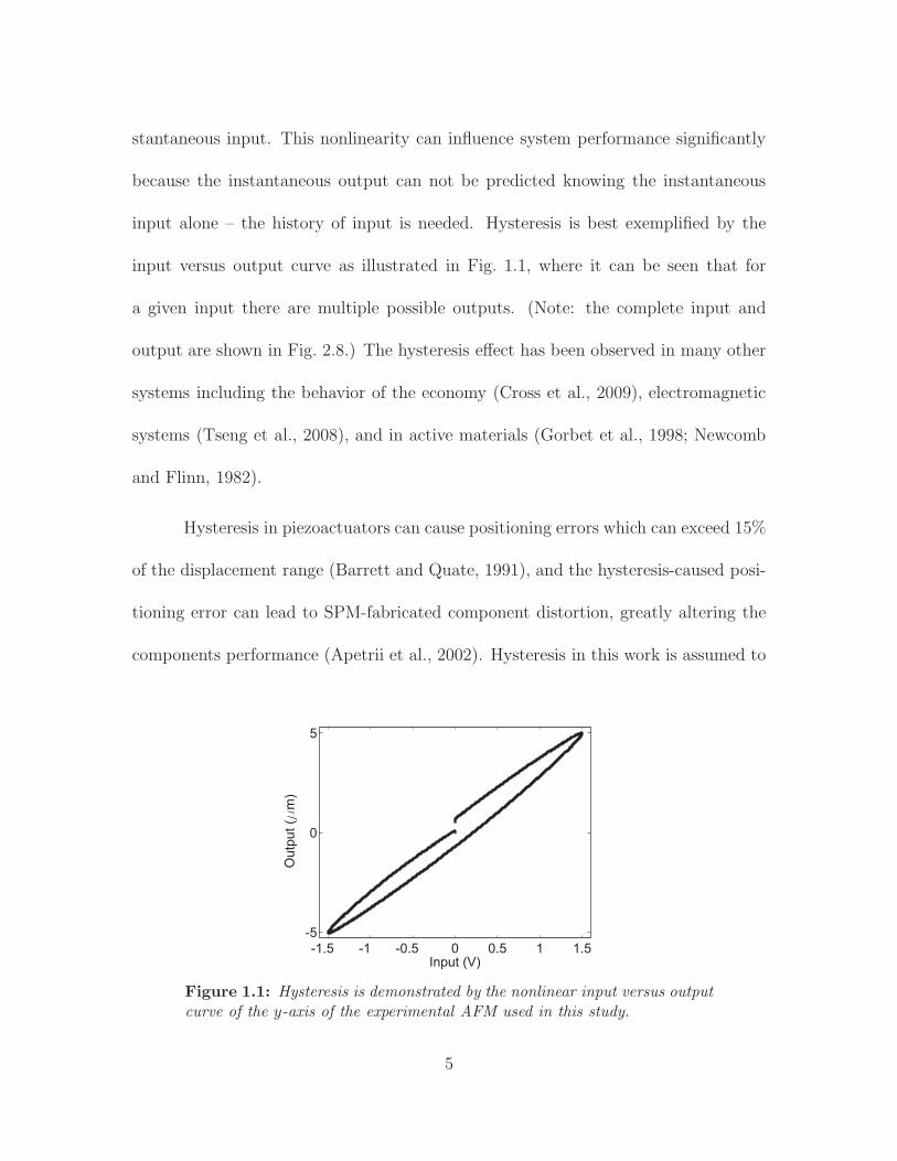
stantaneous input. This nonlinearity can influence system performance significantly
because the instantaneous output can not be predicted knowing the instantaneous
input alone – the history of input is needed. Hysteresis is best exemplified by the
input versus output curve as illustrated in Fig. 1.1, where it can be seen that for
a given input there are multiple possible outputs. (Note: the complete input and
output are shown in Fig. 2.8.) The hysteresis effect has been observed in many other
systems including the behavior of the economy (Cross et al., 2009), electromagnetic
systems (Tseng et al., 2008), and in active materials (Gorbet et al., 1998; Newcomb
and Flinn, 1982).
Hysteresis in piezoactuators can cause positioning errors which can exceed 15%
of the displacement range (Barrett and Quate, 1991), and the hysteresis-caused posi-
tioning error can lead to SPM-fabricated component distortion, greatly altering the
components performance (Apetrii et al., 2002). Hysteresis in this work is assumed to
-1.5 -1 -0.5 0 0.5 1 1.5
-5
0
5
Ou
tpu
t (m
m)
Input (V)
Figure 1.1: Hysteresis is demonstrated by the nonlinear input versus outputcurve of the y-axis of the experimental AFM used in this study.
5

be rate-independent (Yeh et al., 2006), and thus is not affected by the speed at which
the input (such as voltage) is applied. The effects of vibration and creep, although
significant in piezo-based systems, can be minimized by modifying the applied input
speed, and are not considered in this work. The focus in this thesis is hysteresis
compensation using iterative control. However, existing feedback and model-based
feedforward control methods can be applied to address the effects of creep, vibration,
and hysteresis (Clayton et al., 2009) as discussed in the following.
1.4 Piezoactuator Control Approaches
A number of control techniques have been employed to achieve the necessary precision
for applications such as assembling a single-file line of 5 nm diameter silicon nanocry-
tals 60 nm long for electrode repair (Decossas et al., 2003) and dynamically plowing
resist to fabricate 60 nm by 50 nm quantum point contacts (Skaberna et al., 2000).
These control techniques can generally be categorized as either feedback control or
feedforward control (Devasia et al., 2007). In feedback control, which is a reactive
approach, the measured response of the system is fed back and compared to the ref-
erence value, producing an error signal used by the controller. On the other hand,
feedforward controllers, which anticipate deficit performance, use an input which is
predetermined to achieve a particular output or to “cancel” a particular effect.
Feedback controllers have many advantages. Feedback controllers do not re-
quire the actuator to be modeled in detail (Salapaka et al., 2002; Tamer and Dahleh,
6

1994). Feedback controllers are more robust to actuator parameter variations, and
they can overcome disturbances (Boulet, 2000). The drawback is limited operating
frequency (Schitter et al., 2001), as there is often a trade-off between bandwidth and
precision (El Rifai et al., 2003). Finally, feedback gains are limited due to closed-loop
stability issues caused by the inherent low gain-margin of piezoactuators (Leang and
Devasia, 2007; Tien et al., 2005).
Feedforward control methods for hysteresis compensation have been studied
for AFM (Croft et al., 2001). The inversion-based feedforward technique (Clayton
et al., 2009) can provide good tracking performance given an accurate system model.
Unfortunately, as the system ages or environmental conditions change, the system
changes, thus, the model changes (Melnik, 2003). The changing system can lead to
model errors, and model error can have a negative impact on the precision of model
inversion-based feedforward controllers. It has been shown that trajectory tracking
errors caused by model uncertainties (due in part to parameter variations) cannot
be corrected by inversion-based controllers (Zhao and Jayasuriya, 1995). It is noted
that inverse-model feedforward control integrated with feedback has been used to
compensate for hysteresis and other system dynamics and has shown an improvement
over feedback alone (Leang and Devasia, 2007; Song et al., 2005).
The repetitive behavior of a system can be exploited for feedforward hysteresis
compensation (Leang and Devasia, 2006). The AFM often requires the piezoactuator
to operate in a repetitive manner, such as the repetitive lateral motion of AFM
7

imaging. Fabrication techniques are inherently repetitive, as well, to allow for high
throughput and mass-production. This repetition is evident in the proposed use of
AFM in the fabrication of superconducting flux flow transistors (Ko and Kim, 2009),
and in using AFM to fabricate 70 nm wide nano-wire as a hydrogen sensor (Li et al.,
2008). Iterative control (Arimoto et al., 1984) uses this repetitive motion as a basis to
find the input that achieves the desired output. The iterative approach is, practically
speaking, very similar to how humans learn to perform a task. The task is repeated
multiple times, using the error from the current trial to improve the performance of
the next trial.
Several researchers have used iterative control to assist in control of piezo-based
systems (Hinnen et al., 2004; Tien et al., 2005; Wu et al., 2008). In particular, Leang
and Devasia (2006) were one of the first to use iterative control for hysteresis compen-
sation in AFM. They used a proportional-type (P-type) iterative control algorithm
(ICA), where the next iteration’s input signal is the sum of a proportion of the cur-
rent tracking error and the previous input signal. Leang and Devasia (2006) proved
convergence of the algorithm and experimentally showed that the tracking error can
be reduced to nearly the noise level of the sensor measurement. Unfortunately, the
proportional iteration gain is conservative, and, therefore, may require a large num-
ber of iterations before converging to a predefined, acceptable error level. The large
number of iterations motivates the search for a new iterative control algorithm.
8

1.5 Proposed Approach
The focus of this work is to use additional information about the system for itera-
tive control with the objective of improving the convergence rate of the algorithm.
Practically speaking, fewer iterations relates to less time spent waiting for the track-
ing error to be reduced to an acceptable level. In this work, the repetition of AFM
fabrication is exploited to iteratively find an input which allows the AFM to track
a desired trajectory with minimal error by using an input-update law which uses an
inverse-model of the hysteresis. As was described above, others have used an inverse
of a hysteresis model to compensate for the effect of hysteresis in feedforward control.
A benefit of the implementation of the proposed algorithm is the inverse hysteresis
model is derived experimentally, thus the system does not require complex modeling,
to achieve a minimal error in fewer iterations than the standard, P-type ICA (Leang
and Devasia, 2006).
The AFM has been proposed to be used in many fabrication applications
that require micro- and nano-precision positioning, such as the creation of ballistic
quantum devices by dynamic ploughing (Kunze, 2002) or, as previously discussed,
efficient quantum structures. There is a need for control systems that offer nano-
scale precision and are appropriate for automated mass production. Because the
standard, proportional iterative method requires many iterations and in order for
iterative control to be a practical production-level control scheme for SPM-based
systems, it is critical that the number of required iterations to achieve a minimal
9

tracking error is reduced, thus motivating the attempt to exploit the hysteretic nature
of piezoactuators through the proposed ICA. The contribution of this work is the
experimental validation that the proposed algorithm offers comparable precision as
the standard, proportional algorithm, but with fewer iterations to achieve a desired
trajectory which can be used in AFM fabrication.
1.6 Thesis Outline
The remainder of this thesis is structured as follows. Chapter 2 presents a back-
ground on AFM. A history of AFM is presented, including a description of how AFM
works and the components involved. This chapter concludes with a description of
hysteresis, an overview of methods to model hysteresis, and a survey of control meth-
ods others have employed to compensate for hysteresis. In Chapter 3, the iterative
control approach is reviewed, existing iterative control methods are surveyed, and
inverse-hysteresis iterative control is presented in this chapter. The experimental
system used in this work and the details of the experimental iterative algorithm are
introduced in Chapter 4. Experimental results are presented in Chapter 5 for both
the inverse-hysteresis and the proportional iterative control methods for comparison.
The fabrication process with and without iterative control applied is also presented
in this chapter. Concluding comments appear in Chapter 6, and future work is dis-
cussed in Chapter 7. At the end of the thesis, in the Appendix, samples of the C and
MATLAB code used in this work are presented.
10

Chapter 2
The Atomic Force Microscope
This chapter provides an overview of the AFM, a type of scanning probe
microscope. The invention, operating modes, and key components are presented. This
is followed by a review of hysteresis, modeling techniques, and methods to compensate
for hysteresis in AFM.
2.1 History of Microscopy
The invention of the microscope was the necessary first step toward the modern-
day understanding of biology, chemistry, and nano-technology (Rochow and Rochow,
1978). However, it is not known who first used a lens to magnify small objects. In
the first century A.D., a Roman philsopher named Seneca noted, “However small
and obscure the writing may be, it appears larger and clearer when viewed through
a globule of glass filled with water” (qtd. in Allen, 1940). Despite the ancient use
of magnifying lenses, there is little evidence of improvements until the end of the
sixteenth century when a Dutch, spectacle-making father and son team, Hans and
Zacharias Janssen (1580-1683), while experimenting with several lenses in a tube,
discovered that nearby objects appeared much larger (Allen, 1940). This discovery
was the precursor to the compound microscope.
11

In the 1600’s, Antony van Leeuwenhoek of Holland, as an apprentice draper,
used magnifying glasses to count the threads in cloth. He taught himself new methods
for grinding and polishing tiny lenses with significant curvature and magnifications
up to 270x, the best at that time (Huxley, 2007). This led him to the building of
microscopes and the biological discoveries for which he is famous. Leeuwenhoek made
the first observations of microbes, and reported his findings in over one hundred letters
to the Royal Society of England and the French Academy. He is now considered the
father of microbiology (Huxley, 2007).
Robert Hooke, the English father of microscopy, has been called the world’s
first professional scientist (Huxley, 2007). Hooke improved upon Leeuwenhoek’s de-
sign and used it to verify many of his discoveries. In 1665, Hooke wrote Micrographia,
which is considered to be the first book describing observations made through a mi-
croscope (Huxley, 2007). Few major improvements were made to the microscope until
the mid-1800’s when several European countries began to manufacture fine optical
equipment (Allen, 1940), but the desire to explore smaller domains has remained.
An optical microscope, even one with perfect lenses and perfect illumination,
cannot be used to distinguish objects smaller than half the wavelength of the light
used. The smallest wavelength of visible light is approximately 400 nm, thus optical
microscopes, under ideal conditions, have a resolution no less than approximately
200 nm. Because of the desire to explore surfaces at a smaller resolution, methods
were explored to decrease the wavelength of the reflected media.
12
In an attempt to achieve finer resolution, the electron microscope was invented
in the 1930’s by Max Knoll and Ernst Ruska (Ruska, 1987). Ernst Ruska earned half
of the Nobel Prize for Physics in 1986 for the invention. In the electron microscope,
electrons are excited in a vacuum to wavelengths much smaller than visible light.
The electrons are reflected off the surface and a depiction of the sample is created
by detectors at a resolution of approximately 2 nm. In the pursuit of even finer
resolution, other microscopy techniques were explored which no longer depend on
the use of reflection. The scanning tunneling microscope (STM) was one of the
technologies explored.
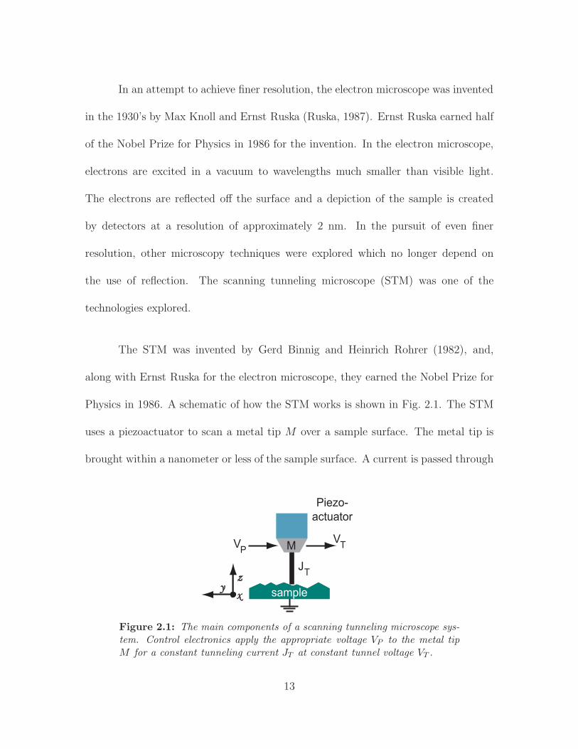
The STM was invented by Gerd Binnig and Heinrich Rohrer (1982), and,
along with Ernst Ruska for the electron microscope, they earned the Nobel Prize for
Physics in 1986. A schematic of how the STM works is shown in Fig. 2.1. The STM
uses a piezoactuator to scan a metal tip M over a sample surface. The metal tip is
brought within a nanometer or less of the sample surface. A current is passed through
Piezo-
actuator
zy
x
MV
TVP
JT
sample
Figure 2.1: The main components of a scanning tunneling microscope sys-tem. Control electronics apply the appropriate voltage VP to the metal tipM for a constant tunneling current JT at constant tunnel voltage VT .
13

the metal tip and forms a tunnel through a vacuum to the sample, hence the name
tunneling microscope. As the piezoactuator moves the metal tip M in the x- and y-
axes, the tunneling current JT changes based on the topography of the sample. Thus,
the piezoactuator moves the metal tip in the z direction to maintain the tunneling
current constant as the tip is scanned along the x and y directions over the sample.
Because a current passes from the scanned metal tip to the sample, a conductive
sample is required - a drawback of STM. The same topographical imaging principle
was later applied to the atomic force microscope.
2.2 Atomic Force Microscopy
The atomic force microscope was invented in 1986 by researchers at IBM and Stanford
University (Binnig et al., 1986) who recognized the need for a technique to examine
insulating surfaces at the atomic scale, and later, atomic resolution images of noncon-
ducting surfaces were achieved (Albrecht and Quate, 1987). The term ‘microscope’
in the name “atomic force microscope” is misleading because it suggests an optical
mechanism. In fact, the information is assembled by “feeling” the surface similar
to how a person reads Braille, moving over the sample surface with a mechanical
probe (Rosenwald, 2010). In this way, the AFM operates in a manner very similar
to the STM. A small cantilever (often approx. 150 µm by 40 µm by 5 µm) has a
tip extending perpendicular to the beam similar to the arm and stylus of a phono-
graph. The tip usually has a diameter in the nanometer range. In AFM imaging, the
14

cantilever is lowered to the surface so that the tip either contacts or nearly contacts
(within nanometers) the surface depending on the mode of operation. The cantilever
is typically raster-scanned, in the x- and y- axes, across the sample (see Fig 2.2)
by a piezoactuator while the tip is moved vertically, in the z-axis, to maintain scan
parameters (discussed further below). The vertical motion matches the topography
of the surface, as shown in Fig. 2.3.
A common AFM design is shown in Fig. 2.4 and consists of a micromachined
cantilever (e.g., see Fig. 4.4) controlled by a piezoactuator. In one mode of operation,
the cantilever tip is brought into contact with a sample surface, while the tip-sample
y -a
xis
x -axis
Image Area
y -a
xis
Time
(b)
Time
x -a
xis
(a) (c)
Figure 2.2: The raster AFM imaging trajectory, as seen from (a) top view,(b) the y-axis, and (c) the x-axis trajectories.
A
AFM Tip
Sample Surface
Figure 2.3: The fundamental operation of the AFM. The tip follows the to-pography of the sample, along path A, to keep scanning parameters constant.
15

Cantilever & Tip
Laser
Photo-detector
Piezo
Tube
Actuator
Detector
and Actuator
Control
Electronics
z
yx
Sample Surface
Figure 2.4: The main components of an AFM system. A piezoactuatormoves a cantilever and tip over the fixed sample surface. A laser reflectingoff the backside of the cantilever, detects the deflection of the cantilever. Thedeflection is monitored and the piezoactuator is controlled by electronics.
forces are monitored. The forces are measured by reflecting a laser beam off the
backside of the cantilever and monitoring the laser’s reflected position with a photo-
detector. As the cantilever bends due to the induced tip-sample forces, the reflected
laser moves on the detector. In commercial systems, a feedback circuit is often used
to maintain a constant tip-sample force. The operation mode that was just described
is contact mode, but, as it has been alluded to, there are several modes of operation
and how the individual components interact depends on the mode.
2.2.1 AFM Modes
In AFM imaging, there are two classes of modes of operation – dynamic and static.
The principle difference is whether the tip is externally excited or not.
16

Dynamic Modes
In dynamic mode, also called non-contact mode, the cantilever is intentionally
vibrated near its fundamental resonant frequency. The amplitude, phase, and fre-
quency of oscillation are influenced by the tip-sample interaction forces. The changes
in oscillation in reference to the driving signal provide information about the sample’s
surface. The most often used dynamic mode strategies are frequency modulation and
amplitude modulation.
When the oscillating tip approaches the sample surface, the tip/sample inter-
action forces cause the amplitude and phase of the of the oscillating cantilever to
change in reference to the driving signal. The changes in the phase of oscillation can
be used to differentiate between surface materials. The changes in amplitude are used
as a topographical map of the surface. The change in amplitude does not happen
instantaneously – the time constant is a function of the Q factor and the resonant
frequency of the cantilever (Giessibl, 2003). Because of the relatively slow response of
amplitude modulation mode, researchers developed frequency modulation (Albrecht
et al., 1991). The frequency of the oscillation, with respect to the applied reference,
varies based on how close the oscillating cantilever is to the sample surface. The
frequency modulation technique has been able to achieve atomic resolution images
(0.6 nm lateral and 0.01 nm vertical) in ultra-high vacuum conditions (Giessibl, 1995).
The amplitude and frequency modulation modes are intended to be non-
contact methods of imaging – the tip is far away (nanometers) from the surface
17

where the forces acting on the tip are attractive. Tapping mode was developed as
an amplitude modulation method in ambient air which operates closer to the surface
(Zhong et al., 1993). The surface is literally tapped by the AFM tip. A more detailed
description of AFM dynamic modes can be found in reference (Giessibl, 2003).
Static Modes
In static mode, also called contact mode, the AFM tip is lowered until contact
with the sample surface is made. There are two distinct contact modes, constant-
force and constant-height. In constant-force mode, the tip is lowered to deflect the
cantilever a given amount, thus applying a known force to the sample. As the tip
is scanned across the sample, the piezoactuator moves the tip perpendicular to the
surface (in the z-axis) to maintain a constant cantilever deflection Dc. The z-axis
motion matches the topography of the sample, and the resulting three-dimensional
image is a map of the function z(x, y, Fts = constant). Unfortunately, this mode is
prone to deforming the surface by scratching if the tip-sample force Fts is too great.
If the tip-sample force is too small, the image will have poor resolution.
In constant-height mode, the piezoactuator maintains a constant height, thus
the cantilever deflects Dc with the sample topography as it is moved over the sample
surface. The three-dimensional image, in constant-height mode, is a map of the
function Dc(x, y, z = constant). Damage to the cantilever and tip, or image distortion,
can occur if a sample feature is too tall, the sample has depressions too deep, or if
the sample surface is not level with the piezoactuator.
18

In summary, with static mode, the cantilever tip is actually in contact with the
sample surface, mapping the surface by keeping the cantilever deflection Dc constant
or the height z of the piezoactuator above the sample constant. Dynamic modes
vibrate the cantilever above the sample surface, monitoring the amplitude, frequency,
and/or phase of the vibration, relative to the applied signal, as the tip-sample forces
interact. Nanofabrication methods have employed both static (Sohn and Willett,
1995) and dynamic techniques (Wilder et al., 1998). Regardless of the mode employed,
precise control is necessary. To achieve precision, an understanding of each of the
components involved is necessary.
2.2.2 AFM Components
The original AFM scanned a foil lever with a piezoactuator across the surface and
measured the deflections of the lever, caused by changes in force, measured through
tunneling currents (Binnig et al., 1986). Each of the main components of the common
AFM – the cantilever, the force sensor, and the piezoactuator – are described here.
The Cantilever
One critical component of the AFM is the cantilever. In this work, the same
component is referred to as the cantilever, lever, tip, or probe.
The first prototype AFM, described by Binnig et al. (1986), employed a gold
foil cantilever with a diamond stylus to help image a sample with a lateral resolution
of 3 nm and a vertical resolution of less than 0.1 nm. The gold foil lever was used
19

because of its low spring constant, minimal mass, and its conductive properties. The
spring constant is necessarily low to allow the maximum deflection to measure the
interatomic forces (between 10−12 N and 10−7 N), but at the same time a stiff spring
with high resonant frequency is desirable to minimize the effects of vibrational noise.
If the mass, m0, is minimized and the spring constant, ks, is minimized as well,
the resonant frequency, fr, can be kept high, because the resonant frequency of the
cantilever spring system is given as fr = (1/2π)√
(ks/m0).
Typically, the cantilevers used in commercial AFM are micromachined from
Si or Si3N4 because they are cost-effective, durable materials that can be shaped to
meet different application-specific requirements. (An image of a typical commercially
available AFM probe is shown in Fig. 4.4.) Low force constants (∼ 1 N/m) and
high resonant frequencies (10 − 30 kHz) are desirable attributes of cantilevers for
contact-mode imaging. Non-contact imaging requires a cantilever with a higher force
constant (∼ 40 N/m) and a higher resonant frequency (∼ 350 kHz). Depending on
the application, AFM-based fabrication may require probes that are stiff or flexible
or, perhaps, coated with a special chemical. Most cantilevers have an integrated tip
with an end diameter of 5 − 20 nm.
The conductive properties of the gold foil cantilever used in initial experiments
allowed the use of an STM to measure the deflection of the lever and tip. The
commercial AFMs in use today do not use an STM as a force sensor, therefore,
the conductive properties are not as relevant. Some AFM applications do require
20

a conductive tip, in which case the probe is often coated in conductive material,
e.g., platinum. Many companies offer AFM probes with a reflective coating on the
backside to aid the force measurement.
The Force Sensor
Because one key component of the AFM system is the sensor used to mea-
sure the forces acting on the tip due to the tip/sample interaction, several different
sensing methods have been used. The laser diode method (Sarid et al., 1988) and an
optical interferometric sensor (Erlandsson et al., 1988) were developed to replace the
tunneling current mechanism used originally. While the tunneling current method
is more sensitive, the simpler optical interferometric sensor system has proven to be
capable of atomic resolution (Binnig, 1992). The optical method is employed in most
commercially available instruments and uses a laser beam reflected off the backside
of the cantilever. The reflected laser strikes a segmented photo-detector. A quarter
Torsional
Deflection
Vertical
Deflection
Photo-
detector
Figure 2.5: A quarteredphoto-detector can detect thetorsional and vertical deflec-tion of the cantilever.
segmentation allows both the vertical and tor-
sional deflection of the cantilever to be detected.
In contact mode, the torsional deflection relates
to the friction of the sample surface. As the tip
moves across the surface, the tip/sample friction
causes the cantilever to twist (see Fig. 2.5) caus-
ing the reflected position on the photo-detector
to move horizontally. This allows sample surface
21

properties to be detected. As the oscillation parameters in dynamic modes and to-
pography in static modes change, the reflected position on the photo-detector changes
vertically, thus, the topography of the sample can be detected.
The Piezoactuator
There are two methods to scan the AFM tip relative to the sample surface –
move the sample relative to a stationary tip, or move the tip relative to a stationary
sample (see Fig. 2.4). The stationary-tip configuration is inherently less versatile,
because of the limitations on the sample. If the sample can fit on the holder, it is
generally expected to change in size and weight, thus the mechanics of motion can be
expected to change. Conversely, the stationary-sample structure allows temperature
and humidity conditions of the sample to be controlled, the sample can be immersed
in an aqueous or gaseous solution without affecting the operation of the piezoactuator,
and the sample surface can be as large as a table top or as small as the range of the
piezoactuator. The AFM used in this work, and many commercial AFMs, employ the
stationary-sample configuration. Both AFM designs typically use a piezoactuator as
the scanning mechanism.
Piezoactuators are used in AFM and SPM because they offer high mechanical
resonant frequencies, low power consumption, they are physically small, have fast
response times (acceleration rates of 98, 000 m/s2 can be achieved (Salapaka et al.,
2002)), and they can generate forces in the kN range. Piezoactuators have operating
temperature ranges from nearly −460 ◦F, with diminished sensitivity (Salapaka et al.,
22

2002), to nearly 250 ◦F (Sayir et al., 2005). They also have limited wear because there
are no moving parts as in a motor assembly. An arguably more important reason for
the use of piezoactuators is that they do not have any backlash or friction, and
therefore offer near atomic resolution (Salapaka et al., 2002).
The motion of the piezoactuator is based on the piezoelectric effect. The effect
is exhibited in crystals and ceramics that generate a voltage when pressure is applied,
and, conversely, produce a stress or strain in response to an applied electric field. It is
the former effect which has been used to harvest electrical energy and power devices
(Mane et al., 2009), but it is the latter effect which is useful in microscopy applications.
There are natural materials, such as quartz, and many man-made materials, such as
PZT (lead zirconate titanate), that demonstrate the piezoelectric effect. In AFM,
typically a tube piezo-ceramic is utilized. The tube has the advantage of allowing
+V
z y
x
Displacement
Figure 2.6: The tube piezo-actuator with properly placedelectrodes allows displacementin all three directions.
motion in all three directions, x, y and z,
through careful placement of segmented elec-
trodes on the surface of the tube. As Fig. 2.6
shows, a piezoactuator is capable of x- and/or
y-axis motion by applying a voltage across elec-
trodes on either side of the tube. Vertical mo-
tion is achieved by applying a voltage across
electrodes on the inside and outside of the tube.
There are many excellent resources which offer
23
more information on the piezoelectric effect (Jaffe et al., 1971; Yang, 2005) and its
application (Preumont, 2006).
Partially because of the atomic resolution that the piezoactuator exhibits, the
AFM has proven to be an important tool in micro- and nano-fabrication (Wiesendan-
ger, 1994). To be able to etch parallel lines 10 nm wide and 15 nm apart (Snow and
Campbell, 1994) requires the ability to control the position of the tip with better than
10 nm lateral resolution. An obstacle to precision control is the effect of hysteresis
in piezoactuators. A review the effects of hysteresis and the modeling and control
methods others have employed follows.
2.3 Hysteresis Modeling and Compensation
The precision control of the piezoactuator, common in SPM, is not a trivial task
(Tamer and Dahleh, 1994). A major reason for the control challenge is the effect of
AC SystemON
OFF
Temp.
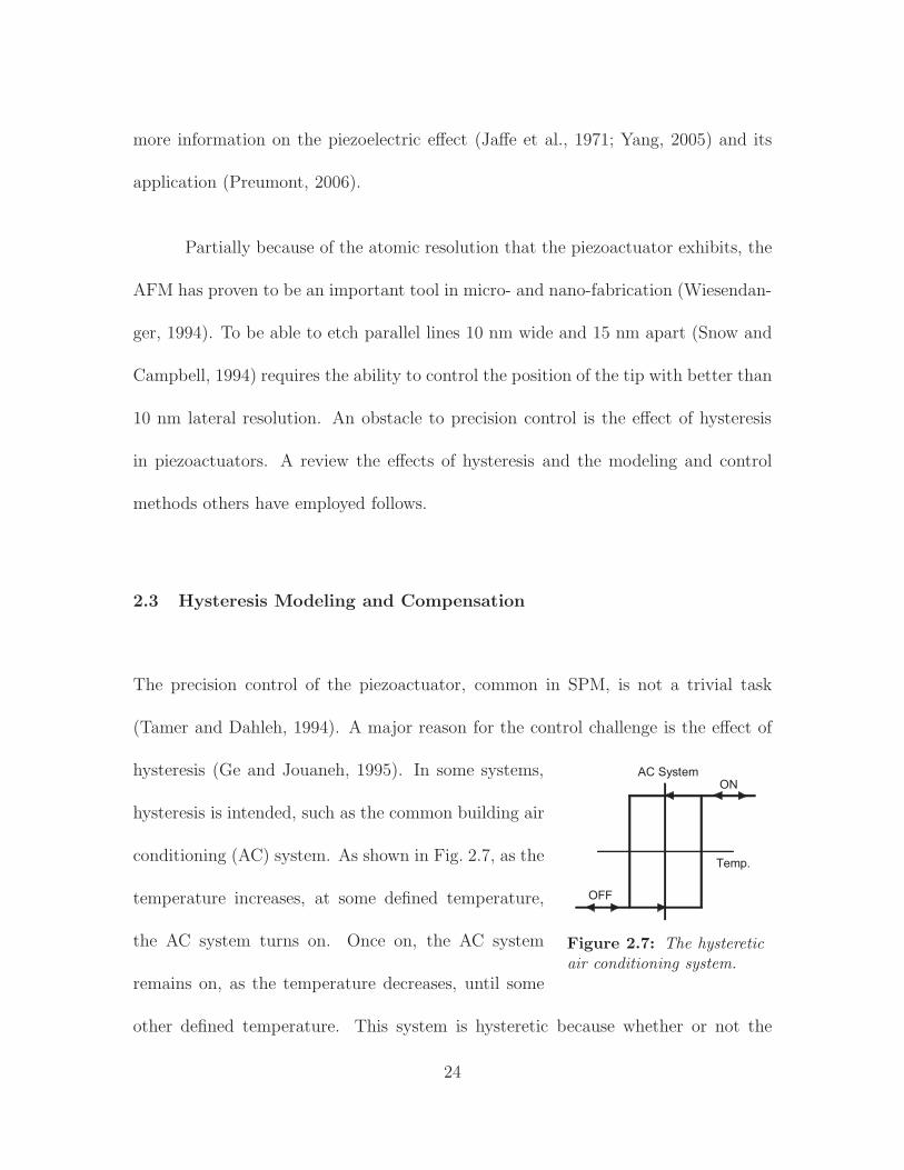
Figure 2.7: The hystereticair conditioning system.
hysteresis (Ge and Jouaneh, 1995). In some systems,
hysteresis is intended, such as the common building air
conditioning (AC) system. As shown in Fig. 2.7, as the
temperature increases, at some defined temperature,
the AC system turns on. Once on, the AC system
remains on, as the temperature decreases, until some
other defined temperature. This system is hysteretic because whether or not the
24
AC system is on depends not just on the current temperature, but on the history of
temperature input as well.
In other systems, such as piezoactuators, the effects of hysteresis are less de-
sirable. For example, in the experimental AFM used in this study, hysteresis can
cause tracking errors in excess of 14% of the displacement range (see Section 5.1).
Because of the dramatic effects of hysteresis, many efforts have been made toward
compensating for it. Before those are discussed, hysteresis is described and modeling
techniques are reviewed.
Hysteresis is a nonlinearity in which the future output depends on the cur-
rent input and output as well as the history of input extremum to the system (Ge
and Jouaneh, 1995). A hysteretic system can be described as a system with a mem-
ory of past input; this memory being nonlinear, discerning, and retentive (Hallett
and Piscitelli, 2002). Within this definition, several terms are significant: nonlin-
ear dependence on past input implies that removing or reversing the input does not
(generally) return the system to its initial state. Retentiveness suggests that the ef-
fects of an input may remain longer than the input was applied. Lastly, hysteresis
is discerning in that not all inputs have an impact: only the latest, more dominant
input.
At any moment in time, the output of a hysteretic system can be in a number
of states (or positions, in the case of the hysteretic piezoactuator), independent of
the current input. This nonlinearity can influence system performance significantly
25

because the instantaneous output can not be predicted knowing the instantaneous
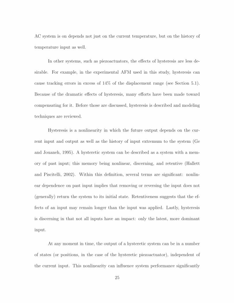
input alone – the history of inputs is needed. The effect of hysteresis in an experi-
mental piezoactuator-based system is illustrated in Fig. 2.8, where a sinusoidal input
is applied and the measured displacement output is shown. The curve in Fig. 2.8(c)
represents the input/output curve of the system (referred to as the hysteresis curve).
It is evident from Fig. 2.8 that for a given input there are multiple outputs that are
possible.
It is the hysteresis curve which illustrates how hysteresis can effect the output
of a piezoactuator. With an input of zero Volts, there is a range of outputs that are
possible, and whether the displacement is 0.7 µm, −0.7 µm, or somewhere in between
depends on the history of past input. Unfortunately, the input history is often not
known or unpredictable. It is the range of possible outputs that make hysteresis
compensation difficult and has inspired the development of many different hysteresis
models to aid control and understanding.
2.3.1 Hysteresis Modeling
Accurate modeling of hysteresis has presented a challenge to researchers for some time,
and many different methods have been used, of varying levels of complexity. Jung
and Kim (1994) have used deterministic models of hysteresis that assume hysteresis
has only local memory to find a feedforward input with a scanning accuracy 10 times
better than open-loop scanning. Hysteresis models which use only local memory
26

0 0.5 1 1.5 2 2.5
-1
0
1
Input (V
)Time (sec)
(a)
0 0.5 1 1.5 2 2.5-5
0
5
Outp
ut (m
m)
Time (sec)
Desired
Actual
(b)
-1.5 -1 -0.5 0 0.5 1 1.5
-5
0
5
Dis
pla
cem
ent (m
m)
Input (V)
14.51% error
(c)
Figure 2.8: Hysteresis as demonstrated by (a) an applied voltage and (b)the measured displacement of the y-axis of the Molecular Imaging PicoPlusAFM experimental system used in this study. The effects of hysteresis arebest illustrated by (c) the nonlinear input versus output curve.
indicate that the future output can be determined by the current value of output and
future input. Therefore, the entire history dependance of the system is contained in
the current value of output (Donnagain, 2004).
A different approach models the hysteresis of the mechanical strain of piezoac-
27

tuators by mathematically expressing the results of the observed phenomena. One
such method was developed by Goldfarb and Celanovic (1997). They used several
generalized Maxwell resistive capacitor elements operating in parallel to represent
rate-independent hysteresis. This modeling strategy requires the measurement of
mass, stiffness, damping, transformer ratio, etc. of the piezoactuator.
In contrast to mechanical strain modeling, other researchers have focused on
different views of the physical phenomena. Simkovics et al. (2000) have considered
dielectric polarization to develop a model using the Preisach hysteresis model (dis-
cussed below) and finite element analysis. Smith and Ounaies (2000) based their
model on the physical domain wall movements and the internal energy losses of the
material. Their method is similar to the Jiles-Atherton model (1984) for ferromag-
netic hysteresis, which is also based on domain wall motion.
Still another modeling method is the micromechanical method. This method
considers the individual dipoles of the actuator, and the hysteresis is modeled by
averaging over all the dipoles in the volume. Delibas et al. (2004) have developed a
micromechanical model which uses 1000 dipoles and probability functions to smooth
the simulated hysteresis curves. Micromechanical methods are computationally ex-
pensive because it is very difficult, if not impossible, to accurately capture the macro-
scopic hysteresis effect by considering individual microscopic dipoles (Hegewald et al.,
2008).
The Preisach model, another phenomenological approach, was first developed
28

to describe hysteresis in magnetic materials (Preisach, 1935), but has been applied
to piezoactuators (Ge and Jouaneh, 1995; Hu and Mrad, 2003). The Preisach model
uses the state of a large number of switching operators to characterize hysteresis,
and has been shown to accurately model piezoactuator hysteresis (Hughes and Wen,
1997). A thorough discussion of the Preisach model and the properties of the model,
can be found in the works of Mayergoyz (1985, 1991) and Ge and Jouaneh (1995).
Along with the methods described above, hysteresis has also been modeled
using a polynomial approximation (see (Croft and Devasia, 1998; Holman et al.,
1995; Hwang et al., 2000; Simion et al., 2006; Sverkunov, 1973)). The polynomial
method describes hysteresis H as a function of the input u, where the output v is
v(t) = H[u](t), and often uses a curve-fitting method to find the parameters of a
hysteresis model polynomial of the type,
H[u](t) = Au(t)3 + Bu(t)2 + Cu(t) + D, (2.1)
where A, B, C, and D are real constants (Holman et al., 1995). This method can
provide very accurate results, but does require that each hysteresis branch is modeled
individually.
The variety of methods developed to model hysteresis indicates the difficulty
encountered modeling it’s effects. Along with the trouble found modeling hysteresis,
researchers have contended with equal difficulty in trying to compensate for it.
29

2.3.2 Hysteresis Compensation
Hysteresis in the y-axis of the piezoactuator used in this study (shown in Fig. 2.8) can
cause positioning errors which can exceed 14% of the displacement range. It is because
of the profound effect hysteresis can have on a piezoactuator’s ability to track a desired
trajectory that many varying techniques have been proposed to compensate for it. For
example, by controlling the charge applied to the piezoactuator, instead of voltage
control, the effects of hysteresis can be reduced, but this leads to increased drift,
saturation problems, and a reduced travel range with the additional cost of specialized
circuitry (Kaizuka, 1989; Main et al., 1995). Additionally, post-scan software image
correction has been proposed to compensate for hysteresis (Barrett and Quate, 1991).
However, this method is not applicable for fabrication purposes, because it is post-
image processing and not real-time control.
In one of the first applications of SPM to fabrication, researchers were able to
achieve sub-micron lateral resolution relying on feedback control (McCord and Pease,
1987). The application of the principles of feedback began with simple machines as
long as 2000 years ago (Mayr, 1970). Since then, feedback systems have become
more sophisticated and accurate. Feedback has been used to compensate for hystere-
sis in many piezoactuator-based systems (Barrett and Quate, 1991; Daniele et al.,
1999; Salapaka et al., 2002; Tamer and Dahleh, 1994; Zhang et al., 2008), and most
commercially available AFMs use PID (proportional, integral, differential) feedback
controllers. There are definite advantages to using feedback controllers.
30

Among the reasons that feedback controllers are used is the fact that they are
insensitive to actuator parameter variations and can overcome disturbances (Boulet,
2000). Feedback controllers treat hysteresis as a disturbance to the system (Goforth
and Gao, 2008), thus they do not require the actuator to be modeled (Tamer and
Dahleh, 1994). Feedback controllers are robust – they can handle changes to the
system due to age or temperature variations. They are also flexible enough to be
able to handle discrepancies in modeling and unmodeled or unknown dynamics can
be compensated (Salapaka et al., 2002).
A drawback of feedback controllers is they are often sensitive to sensor noise
(Li and Mao, 1999), and the noise at high frequency operation reduces the effective-
ness of feedback control (Smith et al., 2002). Another difficulty of feedback control of
piezoactuators is the inherent low-gain margin of the piezo element limits the perfor-
mance of the controller (Salapaka et al., 2002; Schitter et al., 2001), that is, high-gain
feedback often destabilizes the actuator (Main and Garcia, 1997). More intricate
feedback controllers (compared to PID) have been used to increase the bandwidth of
piezoactuators in an attempt to alleviate the gain margin limitations (Salapaka et al.,
2002).
A different control approach is model inversion-based feedforward control. Re-
searchers have used a model of the hysteresis to develop an input which is prede-
termined (fed-forward) to achieve an output which compensates for hysteresis (Croft
et al., 2001; Ge and Jouaneh, 1995; Schitter et al., 2004; Tao and Kokotovic, 1996).
31

In theory, a model-based feedforward approach can offer perfect trajectory tracking.
By developing a model of the hysteresis and inverting the model, an input can be
found which “cancels” the effects of hysteresis. The success of this control method
is dependent on the accuracy of the hysteresis model. Accurate hysteresis modeling
and calculating an inverse requires the gathering of many input/output data sets and
many calculations. This makes accurate modeling computationally expensive and
prone to error (Goforth and Gao, 2008). Additionally, as the system ages or envi-
ronmental conditions change, the system changes, thus, the model changes (Melnik,
2003). The changing system can lead to model errors, and model error can have a
negative impact on the precision of model inversion-based feedforward controllers.
Both feedback and model-based feedforward control techniques have been
shown to be relatively accurate. They have limited the tracking error to a few percent
of the displacement range (Barrett and Quate, 1991; Putra et al., 2007; Salapaka et al.,
2002; Song et al., 2005). With this degree of error, over a 5 µm range, a tracking error
of 50 nm is unacceptable to create 60 nm wide trenches to aid in the fabrication of
semiconductor nano-devices (Cambel et al., 2008), or to create 100 nm wide by 10 µm
long gold electrodes to be used in nano-electronics (Li et al., 2005). One could easily
find many applications were precision of a few percent of the displacement range is
unacceptable. It is because of the lack of precision available through other techniques
that iterative control of hysteresis in piezoactuators was developed (Hu et al., 2008;
Leang and Devasia, 2006).
32

2.4 Summary
A brief history of microscopes, leading to the development of the atomic force mi-
croscope (AFM), was presented in this chapter. The scanning tunneling microscope
preceded the development of the AFM, which is able to image non-conducting sam-
ples and does not require a vacuum. A survey of the operation of AFM was also
presented. A cantilever with a sharp tip on the end is made to move laterally over
the sample surface by the piezoactuator as the probe tip traces the sample surface.
An overview of the modes of operation was presented, as well as a description of the
force sensor, the cantilever, and the piezoactuator involved in the operation.
This was followed by an overview of hysteresis, which has been defined as a
memory of past input, this memory being nonlinear, discerning, and retentive. Several
different methods of hysteresis modeling were also presented. This discussion covered
the polynomial method, which is accurate and simple to compute but requires each
input/output branch to be modeled individually.
Some previous attempts to compensate for hysteresis were also presented.
Feedback control is made more difficult by the inherent low-gain margin of the piezo-
actuator, which restricts the gain of a feedback controller (Tien et al., 2005). Model-
based inversion control techniques, because they are computationally expensive and
prone to model error, are not efficient for production level use (Goforth and Gao,
2008). It is because of the difficulty compensating for hysteresis, that iterative con-
trol was advanced. An understanding of how AFM was developed, the components
33

involved, and the difficulties of hysteresis compensation provide an important back-
ground to iterative control as applied to hysteresis compensation in AFM, which is
described in the following chapter.
34

Chapter 3
Iterative Control for Hysteresis Compensation
In the previous chapter, the AFM and it’s components were described. The
modeling of hysteresis and previous compensation methods were presented as well. In
this chapter, the need for precision positioning control is discussed. This is followed by
a review of iterative control approaches and the development of the inverse-hysteresis
iterative control algorithm for hysteresis compensation in AFM. A description of how
this algorithm is implemented is presented in Chapter 4.
3.1 Motivation
There have been many advances in the use of piezoactuator-based scanning probe
microscopy (SPM) fabrication techniques over the past decades. The SPM has been
used to fabricate novel nano-scale electronics and structures (Taylor et al., 2005;
Wendel et al., 1994), and sensors and devices (Davis et al., 2000). An SPM has been
used to investigate the nanomechanical properties of bacteria by indentation (Wang
et al., 2007). Additionally, AFM has been used to manipulate particles (Decossas
et al., 2003), and help create a nano-CNC machining system (Yan et al., 2007). The
AFM has been used to perform defect and quality control of optical discs (Wei-xian
and Zhuang-de, 2003). Moreover, the AFM has been used to fabricate features by
35

physically indenting and scratching a sample surface (Kunze, 2002). Each of these
applications require precise lateral (x- and y-axis) control of the piezoactuator.
Ballistic devices are a special class of nano-electronic device in which the dis-
tance electrons travel is small enough that they undergo few, if any, scattering events
from electron-electron collisions. Many novel, interesting ballistic devices have been
proposed. Lateral hot-electron transistors have been demonstrated which use closely-
spaced (200 nm) transistor gates to achieve nearly ballistic electron motion (Palevski
et al., 1989). The unique modifications to voltage-current characteristics of semi-
conductor structures are only observable if nano-scale device dimensions are possi-
ble. SPM-based fabrication techniques have been suggested for such ballistic devices
(Kunze, 2002; Sirena et al., 2009; Skaberna et al., 2000). Because of the increasing
need to miniaturize the lateral dimensions of semiconductor electronics, precise lat-
eral control is required to use SPM-based techniques to create the next generation of
electronic devices (Beaumont, 1996).
Precise positioning is also needed to fabricate quantum structures with SPM
(Apetrii et al., 2002). An SPM has been used to indent a semiconductor surface
to facilitate the growth of quantum structures (Murakami et al., 2001; Taylor et al.,
2005). Quantum structures are made more efficient by growing them closer together –
on the order of tens of nanometers in pitch (Krauss, 2005). The luminescent intensity
and energy of quantum systems have been shown to be impacted by a 4 nm deviation
in size and/or spacing (Leonard et al., 1993). Thus, nano-precision lateral positioning
36

of the SPM probe is required to achieve the spacing necessary for the most efficient
quantum structures with desired properties.
The fabrication of single-electron transistors using nanogap electrodes and self-
assembled quantum dots has become possible due, in part, to recent developments in
nanolithography (Jung et al., 2005). Single-electron transistors have shown unique
characteristics such as gate-controlled tunneling magneto-resistance (Hamaya et al.,
2007). The conventional fabrication of single-electron transistors is based on the
chance alignment of a nanogap electrode created with the lift-off technique and ran-
domly placed quantum dots. The fabrication yield of nanogap single-electron tran-
sistors can be improved by using local oxidation with an AFM to fabricate an 80 nm
wide nanogap electrode precisely aligned with a particular 20−200 nm diameter quan-
tum structure (Moriya et al., 2010). Precise control of the AFM probe is required to
fabricate nanogap single-electron transistors in this way.
Unfortunately, hysteresis is a major contributor to the challenge of precise
piezoactuator control (Song et al., 2005). Hysteresis can cause positioning errors in
excess of 10−15% of the displacement range (Barrett and Quate, 1991; Salapaka et al.,
2002). Because the unique properties of ballistic nano-electronic devices rely on nano-
scale fabrication techniques, because the quality of quantum structures is dependent
on size, shape, and spacing, and because the effects of hysteresis can have a negative
impact on piezoactuator positioning, hysteresis can have a profound negative impact
on the quality of SPM-fabricated devices (Apetrii et al., 2002).
37

It is because of the critical need for precision positioning control, that many
efforts have been made to counteract the hysteresis-caused positioning error in the
piezoactuators of SPM (as described in Section 2.3). Iterative control of hysteresis was
developed to meet this need (Hu et al., 2008; Leang and Devasia, 2006). However, the
simple, proportional iterative control algorithm requires many iterations to achieve a
desired output within a given, minimal error. Each iteration relates to time waiting
for the process to complete. In order for iterative control to be a viable production-
level control algorithm, the number of required iterations needs to be reduced. It
is this need that motivates the attempt to find another iterative control algorithm
(ICA) which requires fewer iterations.
A review of iterative control and how it is applied to hysteresis compensation
is now presented. This is followed by the presentation of the new inverse-hysteresis
ICA.
3.2 Review of Iterative Control Methods
The control method under investigation, one which “learns” an input to achieve a
desired goal by trial and error, has been known by several different names – “better-
ment process” (Arimoto et al., 1984), “repetitive control” (Mita, 1984), which now
refers to a different control method (Alsubaie et al., 2008), “iterative learning control”
(Kawamura et al., 1984), and, as it is known in this work, “iterative control”. It is
generally accepted that Uchiymama (1978) was the first publication to discuss the
38

iterative control method, but because it was written in Japanese, it was not widely
known until Arimoto et al. (1984) began researching iterative control.
There are other publications which predate both Arimoto and Uchiyama. In
a patent filed in 1967 (Garden, 1967), an iterative control method is applied to elec-
tric drive units and pneumatic actuators (for details see (Chen and Moore, 2000)).
There was certainly an interest in iterative controllers before Uchiyama and Arimoto
(Mendel, 1966; Mucciardi, 1972; Sklansky, 1966), however Arimoto et al. (1984) is
referenced as initiating iterative control research in English. It is noted that iterative
control is more thoroughly discussed in the works of Moore (1993) and Xu and Tan
(2003).
The purpose of the iterative method is to use the systems repetitiveness to
employ experience to improve the system control performance even with imperfect
system knowledge. The iterative control approach is, practically speaking, very sim-
ilar to how humans learn to perform a task. The task is repeated multiple times,
using the error from the current trial to improve the performance of the next trial.
System
Memory Memory
Iterative
Controller
uk
vk
vd
uk+1
Figure 3.1: A block diagram de-scription of iterative control.
A block-diagram of the general
iterative control method is shown in
Fig. 3.1. An input uk is applied to the
system and also stored in memory. The
system output vk is stored in memory
and compared to the desired output vd.
39

Based on the iterative controller’s input-update law, the next iteration’s input uk+1
is calculated, k is incremented, and uk is again applied to the system. The process
is repeated with the objective being that as the number of iterations increases, the
system output vk gets closer and closer to the desired output vd, such that,
limk→∞
vk(t) = vd(t), (3.1)
for all t in the finite time interval (Moore, 2003). This is, for example, how one
learns to take desired photographs with no prior knowledge. Initially, some default
settings are used, the results are compared to the desired, the settings are adjusted
accordingly, and the process is repeated. Eventually, the settings are learned to
achieve the desired photographic effect. This is also how iterative control is applied
to actuators. Given a desired trajectory, an input is applied, the resulting output is
compared to the desired, and the input is adjusted accordingly in future iterations.
Eventually, an input is found which achieves the desired actuator trajectory. It is
necessary that the desired photographic effect or actuator trajectory is repeated as
the iterative control method finds the settings or input to achieve only the desired
outcome. Thus, if the desired output changes, the iterative process must be repeated
for the new desired outcome. This is a shortcoming of the control method.
The iterative approach is open-loop control in the time domain, but closed-loop
in the iteration domain (Xu and Tan, 2003). In this way, iterative control is similar
to classical feedback control with an important difference (Moore, 1999). The classic
40

feedback strategy uses information about the effect of the input from the current
time instant to compute the input for the next time instant, however the effect of
this decision is not preserved from one iteration to the next. The iterative control
method stores information about the effect of the input at each time instant during
the iteration and uses that information to calculate an improvement of the input to be
applied during the next iteration. An ICA intends to find an input ud which achieves
a desired output vd by using information about how the controlled system responds
to input over multiple iterations.
Iterative control makes several important assumptions (Ahn et al., 2007).
First, it is assumed the system operates repetitively, each iteration operates over
a finite, fixed time, e.g., t ∈ T , [ti, tf ], and that system dynamics are not altered
throughout each iteration. Iterative control finds an input ud(t) that produces the
desired output vd(t). As such, it is assumed the the input ud(t) exists. It is further
assumed, every output vk(t) can be measured, and, therefore, the position tracking
error signal, ek(t) , vd(t)− vk(t), can be used to determine the next iteration’s input
uk+1(t). Lastly, it is necessary and assumed that the system is set to the same initial
conditions at the beginning of each iteration.
If these assumptions and conditions are met, there are several advantages of
iterative control over other control techniques (Moore, 1993). First, accurate model
information is not necessary to design an accurate iterative controller. An ICA can be
designed, and mathematically proven, to achieve perfect tracking of a desired trajec-
41

tory over a finite time interval. Lastly, if convergence conditions are met, damage to
the hardware can be prevented, the system can converge to a desired trajectory, and
the desired trajectory can avoid being overshot. Partially because of these advantages,
several different iterative control structures have been considered.
Arimoto et al. (1984) proposed what has come to be known as an “Arimoto-
type” input-update law (Ahn et al., 2007),
uk+1(t) = uk(t) + Γek(t). (3.2)
This type of ICA can also be called a “D-type” algorithm because it considers the
derivative of the error. Arimoto et al. (1984) also proposed a “PID-type” ICA,
uk+1(t) = uk + Φek(t) + Γek(t) + Ψ
∫
ek(t)dt, (3.3)
so called because of the proportional Φ, integral Ψ, and derivative Γ gains. A simpler,
proportional, “P-type” algorithm, with no integral or derivative elements, of the form,
uk+1(t) = uk(t) + Φek(t), (3.4)
has also been considered (Dou et al., 1996; Hoelzle et al., 2008; Leang and Devasia,
2006). In each of the above iterative control input-update laws (3.2, 3.3, 3.4), the
iteration gains Φ, Ψ, and Γ are all real constants. These three iterative control
42

algorithms, “D-type”, “PID-type”, and “P-type”, form the bases from which other
algorithms are derived.
As stated above, a requirement of iterative control is that the controlled system
must offer repetitive operation over a finite time interval. Fortunately, there are many
systems, such as nanomanufacturing (Doumanidis, 2004), which function repetitively.
The iterative control method has been applied to chemical processes (Choi et al.,
1996), robotics (Kawamura et al., 1984), generator excitation control (Yu et al., 2008),
magnetostrictive actuators (Song et al., 2006), industrial production machines (Wei
and Panaitescu, 2008), the problem of basketball shot control (Xu et al., 2007), and
vibration isolation (Hao et al., 2008). Iterative control of the proportional type has
been used to automatically tune a feedback controller (Tan et al., 2009). Additionally,
a P-type, phase-lead iterative control scheme, which uses an iteration error ek(z + λ)
computed from time samples a finite number of time samples λ ahead of the currently
considered time sample z (a method developed for non-minimum phase plants), has
been used to apply functional electrical stimulation to the triceps of rehabilitation
patients to assist them in performing trajectory tracking tasks (Freeman et al., 2009).
Iterative control has been applied to piezoactuators. Wu et al. (2008) do not
mention hysteresis directly, but employ proportional-gain iterative control in the fre-
quency domain along with an H∞ feedback controller to control the z-axis of a piezo-
actuator to assist high-speed imaging. They were able to show improved performance
over PI-feedback control alone. Yen et al. (2009) also do not mention hysteresis, but
43

introduce a P-type, multiple-input-multiple-output ICA for a novel optical scanning
system using two piezoactuators to manipulate a mirror. Helfrich et al. (2008) use it-
erative control and H∞ feedback control together to alleviate possible non-repeating
disturbances and iteration initialization errors in piezo-driven nanopositioning sys-
tems.
Iterative control algorithms have been developed for different classes of sys-
tems, including, as mentioned, a phase-lead algorithm for non-minimum phase sys-
tems (Cai et al., 2007; Freeman et al., 2007), a proportional-gain method for dynami-
cal systems (Sugie and Ono, 1991), a D-type approach for nonlinear systems (Su and
Kermiche, 1989), and a P-type algorithm for a linear system (Fan and Liu, 2007).
The iterative control method has also been used to compensate for hysteresis.
An ICA was applied to electromagnetic actuators (Tseng et al., 2008) and electrostric-
tive actuators (Hu et al., 2004). An anticipatory ICA was developed for hysteretic
systems in general (Hu et al., 2008), and a P-type algorithm was applied to com-
pensate for hysteresis in shape memory alloy systems (Ashley et al., 2006) and the
piezoactuators of AFM (Leang and Devasia, 2006).
In summary, the iterative control methodology makes several key assumptions,
including that every iteration operates over a fixed time interval and each iteration
begins from the same initial conditions. The benefits of the iterative control method
include that an accurate controller can be designed with inaccurate system model
information and that if convergence conditions are met, the output of successive
44

iterations will converge to the desired trajectory. There are several general methods of
iterative control, of which the simple, P-type algorithm is one, and the iterative control
system has been applied to many different systems. This work uses iterative control
to compensate for hysteresis, therefore, in the following section, the previous methods
of iterative control applied to compensate for hysteresis are discussed further.
3.3 Iterative Compensation of Hysteresis
Iterative control has been applied to many different classes of systems, and has been
used to control many different actuators and processes. In this section the iterative
methods of compensating for hysteresis are presented. This includes a discussion of
the proportional iterative control on which this thesis is based.
In the work of Tseng et al. (2008), iterative control is used to compensate for
hysteresis in electromagnetic actuators found in magnetic hard-disk recording devices.
They employ a higher-order ICA, which uses data from multiple previous iterations,
uk(t) = αk
∑
i=0
ei(t), (3.5)
where uk is the current iteration input, ei(t) is the tracking error of the ith iteration,
and α is a constant. They relate the hysteretic actuator to an ideal linear actuator
which can be controlled with the function
u(t) = αe(t). (3.6)
45

By relating Eqs. (3.5), (3.6), and subsequent tracking error, ek+1(t) = vd(t) − vk(t),
Tseng et al. conclude that for convergence the iteration gain α is limited as follows,
α max0<u<u
dϕ
du
< 0.5, (3.7)
where ϕ is a function which describes the difference between the actual hysteretic
actuator and the ideal. With the ICA (3.5), Tseng et al. (2008) have shown to provide
trajectory tracking within approximately 2% of the actuator’s range. This level of
precision is not satisfactory for nanotechnologies. Over a 5 µm range, a 2% error
is 100 nm, which is just entering what is normally considered nano-scale precision
(Lizama, 2008).
Hu et al. (2004) have used the iterative control architecture to compensate
for hysteresis in electrostrictive actuators, a relatively new class of smart materials.
In electrostrictive actuators, the induced strain is proportional to the square of the
applied electric field, and, compared to piezoactuators, demonstrate a small amount
of hysteresis (Hues et al., 1994). Hu et al. use a gain-variable feedback ICA, such that
the proportional gain is varied based on the previous iteration result and the assumed
quadratic input/output relationship of the hysteretic actuator. They are able to show
an improvement from 4% tracking error to within 0.5% error in 5 iterations.
An anticipatory iterative control algorithm has been applied to hysteretic sys-
46

tems (Hu et al., 2008) and takes the form
uk+1(t) = uk(t) + L(·)(vd(t + ∆) − vk(t + ∆)), (3.8)
where L(·) is a function chosen by the designer and ∆ > 0 is a small number. In the
work of Hu et al., the input, u(t) = ufb(t) + uic(t), is a combination of a feedback
controller ufb(t) and the feedforward anticipatory input uic(t) updated using Eq. (3.8).
In the simulations presented, the iteration gains lp = 40 and lv = 10 are chosen, but
the function L(·) is not stated. The simulated results show that ICA (3.8) reduces
hysteresis-caused RMS error from 1.2% to less than 0.1% in five iterations.
In the work of Leang and Devasia (2006), convergence was proven for a P-type
ICA to compensate for Preisach-type hysteresis. They use an input-update law of
the form
uk+1(t) = uk(t) + ρ(vd(t) − vk(t)), (3.9)
with an iteration gain ρ and a given desired trajectory vd(t) for all t in the finite
interval. They have shown that convergence is guaranteed if the iteration gain ρ
meets the condition
0 < ρ ≤ min
min{ 1
η2
,2
η1
}
, if n = 1,
min{ 1
η2
,2
η1∆umax
}
, if n = 2,
(3.10)
where ∆umax is the maximum input error and the constants η1, η2, and n are deter-
47

mined from the input/output relationship, the Preisach model, and properties thereof.
The iteration gain ρ is necessarily conservative to ensure that the desired trajectory
vd(t) is not overshot and, therefore, monotonicity of input and output are maintained,
which ensures that the direction to change the input is known based on the output
error (Leang and Devasia, 2006). The proportional ICA (3.9) was applied to the
piezoactuator of an AFM to achieve an imaging trajectory, and has shown a tracking
error reduction from 7.15% to less than 0.25% of the displacement range – which
is nearly the noise level of the displacement measurement sensor – in 40 iterations
(Leang and Devasia, 2006). The same methodology and principles were applied to
hysteresis-compensation of a shape memory alloy (Ashley et al., 2006).
The work of Leang and Devasia (2006) forms the basis of this thesis. A benefit
of the proportional ICA to compensate for hysteresis is, if the iteration gain ρ is chosen
to be sufficiently small, an input that achieves a desired output can be found with
minimal information about the system – the desired trajectory must be continuous,
monotonic, and belong on a single branch. It is because the iteration gain ρ is
necessarily conservative, that at some points along the desired trajectory convergence
comes more quickly than at other points. Thus, the entire algorithm must wait for
the slower points to ultimately converge. This implies that the ICA (3.9) requires
a greater number of iterations than otherwise required. The number of iterations
required to achieve a given, minimal error relates directly to the time spent waiting for
the process to complete. This is the motivation for a new iterative control algorithm.
48

3.4 Inverse-Hysteresis Iterative Control
In the previous section, some of the past methods of applying iterative control to
compensate for hysteresis were investigated. The work of Leang and Devasia (2006)
has successfully shown how to track a desired trajectory with minimal error, but at
the expense of many iterations. In this section, the development of the proposed
iterative control algorithm is examined. In the following chapter, the experimental
system and the experimental implementation of the proposed ICA are reviewed.
The constant gain ρ of ICA (3.9) is necessarily conservative and may lead to
slow convergence. For example, when the iterative algorithm (3.9) was applied to
a hysteretic shape memory alloy system, more than 500 iterations were required to
achieve 20% error (Leang et al., 2009a). The number of iterations required to achieve
a predefined minimal error relates directly to the time spent waiting for the process
to complete. In the experimental system used in this thesis, each iteration requires
more than one minute. Thus, even a 10% improvement in the number of iterations
required, can mean real time savings. To improve the performance of iterative control,
the system model is exploited.
In order to find the desired input ud which achieves the desired output vd, it is
desirable to have the input of the next iteration be the input which realizes the desired
output. Thus, we want uk+1(t) = ud(t) for all time t in the finite interval T . Based on
references (Devasia, 2000; Iyer et al., 2005; Smith, 2001), among others, the hysteresis
model H has been inverted to find a feedforward input to compensate for hysteresis.
49
Several hysteresis model structures in particular have been shown to be invertible.
A polynomial-based hysteresis model has been inverted to find a feedforward input
to a piezoactuator (Croft and Devasia, 1998), and an inverse Preisach hysteresis
model has been used to find a feedforward input along with PID feedback control
of a piezoactuator (Song et al., 2005). The hysteresis model is, therefore, assumed
invertible.
Given an invertible model, for a given desired output vd(t) = H[ud](t), the
input ud(t) which achieves the desired output can be found by calculating the inverse
hysteresis model H−1. Therefore, given an assumed invertible hysteresis model,
vd(t) = H[ud](t) ⇐⇒ ud(t) = H−1[vd](t), (3.11)
vk(t) = H[uk(t)] ⇐⇒ uk(t) = H−1[vk](t). (3.12)
Thus, using an inverse model of hysteresis, and starting with the fact that it is
desirable to have the next iteration’s input be the input which achieves the desired
output, an iterative control input-update law can be written as,
uk+1(t) = ud(t),
uk+1(t) = uk(t) + ud(t) − uk(t),
uk+1(t) = uk(t) + H−1[vd](t) −H−1[vk](t). (3.13)
If a perfect hysteresis model H can be identified, a perfect inverse model H−1
50

can be found, and with input-update law (3.13), convergence can be achieved in one
step. In practice, however, the model will have uncertainty. To aid in accounting for
this uncertainty, simply, the constant α is introduced,
uk+1(t) = uk(t) + α(
H−1[vd](t) −H−1[vk](t))
, (3.14)
for all time t in the finite interval T .
In the work of Ashley, Aridogan, Riddle, and Leang (2008), it has been proven
that for convergence of ICA (3.14), the following must be true,
1. The hysteretic behavior of the piezoactuator and the hysteresis model used are
invertible.
2. Before each iteration, the initial conditions are made the same. That is, the
input and memory of past input are the same at the beginning of each and
every iteration.
3. The desired trajectory is continuous and monotonic for all time in the finite
interval considered.
4. The constant α is limited by
0 < α ≤ min
{
ξ1
(ξ2 + M), 2
}
, (3.15)
where ξ1, ξ2, and M are real constants based on, and derived from, the in-
put/output relationship. The details of this limitation on the iteration gain α
are presented in reference (Ashley et al., 2008).
51

3.5 Summary
In summary, precision control of the piezoactuator in AFM is required to produce
the next generation of electronic devices and to fabricate the most efficient quantum
structures with desired properties. Because of this need for accurate lateral position
control, the drastic effects of hysteresis, the complexity of model inversion-based
control techniques, and the gain limitations of feedback control, iterative control of
the piezoactuator in AFM was developed.
Iterative control has been applied to many different systems and classes of sys-
tems – from actuators to vibration control systems and from dynamic to non-minimum
phase systems. Different iterative methods have been applied to such varying sys-
tems partially because accurate system information is not required to design and use
an accurate iterative controller. An additional advantage of iterative control is that
if convergence conditions are met, the system will, in practice, approach perfectly
tracking a desired trajectory.
An ICA makes several key assumptions about the behavior of the system and
the execution of the controller. An iterative controller assumes that before each
iteration begins, the system is in the same initial condition or position. This is
very important to the execution of an ICA used to compensate for hysteresis and is
discussed further in the following chapter.
Several iterative control methods have been employed to counteract the effects
of hysteresis. A proportional, fixed-gain algorithm has shown AFM control of the pre-
52

cision needed for applications such as the fabrication of efficient quantum structures.
Unfortunately, because of the necessarily conservative iteration gain, the algorithm
requires many iterations, and therefore time, to achieve such precision. This is the
reason for the development of the new ICA (3.14) which exploits the hysteretic na-
ture of piezoactuators in the input-update law. Before the results of the experimental
validation of the ICA (3.14) are presented, the experimental system and the empirical
hysteresis model used are described in Chapter 4.
53

Chapter 4
Experimental System and Implementation
The AFM has been used in the past to fabricate features for the creation of
novel nano-scale electronics, structures (Wendel et al., 1994), sensors, and devices
(Davis et al., 2000). The AFM has also been used to fabricate features by physi-
cally indenting and scratching the surface (Kunze, 2002). In this thesis, the process
of scratching features on a soft sample by physically embedding and “dragging” the
AFM tip over the surface is considered. This approach is one of the simplest fab-
rication techniques and the resulting features can be used in nano-imprint template
fabrication, in high-end photomask repair (Peng et al., 2009), or to define a mask for
lithography to create quantum devices (Wendel et al., 1994), which, as noted in the
previous chapter, are made more efficient by precise lateral placement of the devices.
As presented in Chapter 3, the proportional iterative control algorithm (3.9)
has been used to achieve precision lateral control of the piezoactuator in AFM (Leang
and Devasia, 2006), but requires many iterations to attain that success because of the
necessarily conservative iteration gain ρ. Based on the conservative nature of propor-
tional iterative control, the new, inverse-hysteresis iterative control algorithm (3.14)
was developed. As proof of the effectiveness of the proposed iterative control algo-
rithm (ICA), the method is applied to the piezoactuator of an AFM. The desired
54

trajectory vd is a circle in the x/y plane. The circle is scribed in the surface of
a polycarbonate substrate to demonstrate the applicability of the inverse-hysteresis
ICA (3.14) to a fabrication process. To demonstrate its improved performance, the
inverse-hysteresis ICA is experimentally compared to the proportional ICA.
The first section of this chapter details the experimental system used. This is
followed by a discussion of how the inverse-hysteresis of the desired trajectory vd and
each iterations output vk are empirically gathered and calculated and how these are
used in the overall iterative control process.
4.1 Experimental System
4.1.1 System Overview
The experimental AFM system used in this thesis is the Molecular Imaging (MI,
now part of Agilent Technologies, Chandler, AZ) PicoPlus model. In this AFM, the
cantilever probe is attached to a sectored tube piezoactuator, or piezo-positioner,
which moves the cantilever relative to a fixed sample plate as shown in Fig. 4.1. An
image of the Agilent Technologies 5500 AFM, which replaced and is identical to the
MI PicoPlus model used in this study, is shown in Fig. 4.2. The Agilent Technologies
datasheet for the piezoactuator scanner used in this study states that the x- and y-
axes have a range of 90 µm × 90 µm and a resolution of better than 5 A. The z-axis
has a range of 7 µm and a resolution of better than 0.5 A. The scanner uses a reflected
laser/photodiode force sensor, and inductive piezoactuator position sensors.
55

Piezo-PositionerOptical
Sensor
Laser
Sample Plate
Polycarbonatexy
z
x Axis
Position
Sensor
y Axis
Position
Sensor
z Axis
Position
Sensor
Figure 4.1: A schematic of the main components of the experimental AFMsystem.
A
B
C
Figure 4.2: A photograph of the 5500 AFM courtesy of Agilent Technolo-gies, Inc. The main components – the piezoactuator, cantilever, inductiveposition sensors, and the optical force sensor – are within (A) the scanner;(B) the sample plate; and (C) an environmental chamber was not used inthis study.
The system is customized with a module to permit access to the control signals
of all three coordinate axes (x, y, and z) of the piezoactuator. The output of the in-
ductive sensors, which are used to measure the displacement of the piezoactuator, are
accessible through the same custom signal access module. The gain of the inductive
56

sensors are 3.59 µm/V in the x-axis and 4.04 µm/V in the y-axis.
To input control signals to the AFM system, an IBM computer with a National
Instruments data acquisition system is used. The same system is used to read the
output position sensor voltages. A custom C-language code (using a Borland Turbo
C DOS compiler) was written to execute the control algorithms. (See the Appendix
for an example of the code used.) The commercial MI software, with a proportional-
integral (PI) feedback controller, is used to image the sample and to control the z-axis
during fabrication in order to maintain a constant deflection of the cantilever, and
thus tip force on the sample. A block diagram of the experimental system is shown
in Fig. 4.3.
C:\
PicoPlus
Piezo
Amplifier
Piezo-
Positioner
z
y
x
x y Volts
Volts
x
y
Cantilever Deflection IMAGING
SYSTEM
Inductive
Sensor
Inductive
Sensor
Inductive
Sensor
z
y
x
Displacementz
y
x
Volts
z
y
x
Volts
x y z
FABRICATION
SYSTEM
Figure 4.3: A block diagram of the experimental AFM system. The MIPicoPlus software is used to image and to establish a constant deflectionof the cantilever during fabrication. An external computer, running customcode, is used to implement the iterative control algorithm, apply controllingvoltages, and measure the displacement of the x- and y- axes.
57

The cantilever used is the NANOSENSORSTM non-contact/tapping mode
probe from the PPP-NCH series, which has a resonant frequency of 330 kHz. This
probe is used partially because of its high force constant of 42 N/m. The cantilever
is made of silicon, has a gold reflective coating on the backside for improved force
sensing, and a tip end diameter of approximately 7 nm (see Fig. 4.4).
Imaging is performed using constant-height, contact mode, as described in
Chapter 2. With the z-axis feedback controller engaged, the cantilever is lowered to
contact the sample surface. The z-axis PI closed-loop control gains are then lowered,
while the x- and y-axis closed-loop control gains are preserved, so the piezoactuator
maintains the cantilever at a constant height above the sample. The piezoactuator
then raster scans the tip across the sample, and the cantilever deflection provides
sample topography information. Imaging is used in this study to verify fabrication.
4.1.2 Frequency Response of the Piezoactuator
While it is usually desirable to fabricate with high throughput, the focus of this thesis
Figure 4.4: A scanning electron microscopy image of the underside of theAFM probe used in this study courtesy of NANOSENSORSTM.
58

is the hysteresis effect; therefore, the AFM is operated at low frequencies to avoid
exciting the high-order dynamics (Mokaberi and Requicha, 2008). To be certain of
this, the frequency response of the piezoactuator is measured for both the x- and y-
axes. The response is measured by applying a sinusoidal input of constant amplitude
(100 mV < 0.5 µm) and varying frequencies (10 Hz – 10 kHz) using a Hewlett
Packard dynamic signal analyzer. The dynamic signal analyzer applies the actuating
signal and records the magnitude and phase (with respect to the applied signal) of
the displacement by way of the inductive sensors. The measured frequency response,
shown in Fig. 4.5, reveals dominant resonant peaks at 415 Hz and 404 Hz for the
x- and y- axes, respectively. Based on the frequency response and to not excite the
high-order dynamics, the fabrication process is chosen to be performed at 0.4 Hz.
4.1.3 The Fabrication Process
To illustrate the iterative control approach for fabricating a feature using the scratch-
ing technique, a simple circular trajectory in the x/y plane was chosen (see Fig. 4.6).
A relatively soft, polycarbonate surface was chosen as the medium for scratching.
The polycarbonate sample has an elastic modulus of 2400 MPa, compared to more
than 60 GPa for the silicon cantilever (McSkimin, 1953).
The fabrication process begins by first lowering the AFM tip onto the sample
surface, and once in contact with the sample, a relatively low force set point (approx.
0.5 µN) was used to image the sample. The imaging was performed under closed-loop
59

101
102
103
104
-40
-20
0
415 HzM
ag
nit
ud
e (
dB
)
Frequency (Hz)
(a)
101
102
103
104
-1500
-1000
-500
0
500
Frequency (Hz)
Ph
as
e (
de
gre
es
)(b)
101
102
103
104
-40
-20
0
Mag
nit
ud
e (
dB
)
Frequency (Hz)
404 Hz
(c)
101
102
103
104
-1500
-1000
-500
0
500
Frequency (Hz)
Ph
as
e (
de
gre
es
)(d)
Figure 4.5: Frequency response of the piezoactuator of the experimentalAFM system: the (a) magnitude and (b) phase versus frequency about thex-axis; (c) magnitude and (d) phase about the y-axis.
60

0 1.0 2.0 2.95
0
5
Time (sec)
Desire
d T
raje
cto
ry (
mm
)xy
-5 0 5-5
0
5
x ( mm)
y ( m
m)
(a) (b)
Figure 4.6: The desired trajectory in (a) the x- and y- axes and (b) a topview of the desired circular fabrication trajectory.
PI control (ki = 1.2, kp = 1.0) using the MI software. Closed-loop imaging was done to
obtain an accurate image of the surface, especially to verify the success of fabrication.
After imaging, the piezoactuator was brought to the home position (x = y = 0)
and the force set point was increased to approximately 7.5 µN for scratching. It is
noted that the value agrees with the work of other researchers, for example see (Yan
et al., 2007, 2005). With the tip fully engaged, control voltages were then applied to
the x- and y- axes of the piezoactuator from the external computer running custom
C code. Once fabrication was complete, the force set point was reduced to the same
0.5 µN force set-point to image (in closed-loop) the sample for verification of the
fabrication process. The x and y trajectories input to achieve the desired output are
iteratively “learned” through the application of inverse-hysteresis ICA (3.14), which
is described in the following section. It is noted that in order to meet the iterative
control requirement that system dynamics do not change throughout each iteration,
the iterative process was implemented with the AFM tip not in contact with the
sample surface, that is, hovering micrometers above the sample.
61
4.2 Iteration Process
As was described in Chapter 2, others have used the inverse of the hysteresis model
to compensate for the effect of hysteresis (Croft et al., 2001; Ge and Jouaneh, 1995;
Schitter et al., 2004; Tao and Kokotovic, 1996). A drawback of this approach, is
that modeling errors negatively affect the performance of the controller. A benefit of
the implementation of the proposed algorithm (3.14) is the inverse hysteresis model
H−1 is derived experimentally. The exact steps of the proposed algorithm are first
outlined, followed by an explanation of how the inverse hysteresis data is acquired
and then used.
4.2.1 Overview of Process Steps
The inverse-hysteresis iterative control process begins by dividing the desired trajec-
tory vd, with a total of N monotonic sections, into each monotonic section n. The
next step is to gather hysteresis data (open-loop input/output data) for the section
being iterated. With the hysteresis data, the iterative control algorithm really begins.
This is outlined in the steps below.
1. Manually divide the desired trajectory vd into N individual monotonic sections.
2. Ramp the input to gather hysteresis data.
3. Calculate and store H−1[vd](t).
4. Reset and clear the memory of previous input to satisfy the iterative control
assumption that the initial conditions are the same.
62

5. Apply the input uk(t) and measure the output vk(t) for all time t of the current
monotonic section.
6. Calculate the iteration output’s inverse-hysteresis H−1[vk](t).
7. Calculate the next iteration’s input, uk+1(t) = uk(t)+α(H−1[vd](t)−H−1[vk](t)).
8. Determine if vd(t)− vk(t) is less than the predefined acceptable error ε for each
data point of the nth partition.
(a) If max{|vd(t) − vk(t)|} > ε, increment k and return to step 4.
(b) If max{|vd(t) − vk(t)|} ≤ ε, move on to step 9.
9. Determine if the monotonic section just iterated is the final section. If n < N ,
return to step 1, otherwise the process is complete.
Details of each of the above steps follow.
4.2.2 Partitioning The Desired Trajectory
As was discussed in Chapter 3, the proposed ICA (3.14) requires a monotonic desired
trajectory vd to be able to iteratively find an input ud that achieves the desired
trajectory. However, an input ud that achieves a more general desired trajectory vd
can be iteratively found by dividing the general desired trajectory into monotonic
sections and then iterating on each monotonic section to find the general input ud.
The details of the process and how it works is described in reference (Leang and
Devasia, 2006). The first step in iterating the general desired trajectory vd is to
manually partition the entire general trajectory into individual monotonic sections.
Therefore, the desired x- and y-axis trajectories to realize the circular path used in
63

0 1 2-5
0
5
Time (sec)
Dis
pla
ce
me
nt
(m m
)two
one
three
four
0 1 2-5
0
5
Time (sec)
one
two
three
Dis
pla
ce
me
nt (m
m)
(a) (b)
Figure 4.7: The desired (a) x- and (b) y-axis trajectories partitioned intomonotonic sections.
this study are partitioned into monotonic sections as shown in Fig. 4.7. It is noted
that this method of iterating one monotonic section at a time could be used to achieve
other, non-circular, multi-branch trajectories.
4.2.3 Gathering Hysteresis Data
Before the iteration process is truly begun, the open-loop input and output data
are collected to be used to calculate the inverse hysteresis of the desired and each
iteration’s output. The C program customized to implement the inverse-hysteresis
ICA (3.14) inputs a ramping signal to gather both the input and output data. The
ramp input is increasing if the section being iterated is monotonically increasing, or
decreasing if the section being iterated is monotonically decreasing. As an illustration,
the input versus output relationship of the increasing y-axis input is shown in Fig. 4.8.
64

Because there are two different scenarios for ramping the input to gather the
hysteresis data, depending on whether the current section being iterated is monoton-
ically increasing or decreasing, the latter case is described here, and the negative of
what is described is applied in the former case.
First, the piezoactuator is commanded to follow the input uprev which achieved
the output of the previous monotonic section vprev within the predefined error ε.
When the piezoactuator reaches the end of the previous monotonic section, the input
is increased an additional 0.25 V. A ramping input is then applied which begins with
a value of (uprev+0.25) and ends with the value −(uprev+0.25). The additional 0.25 V
at the extremum of the ramp input ensures the hysteresis data covers the possible
spectrum of minimum to maximum output, that is, the extrema of the ramping input
exceeds the extrema of the input which will achieve this monotonic section.
While the ramp input is applied, both the input and output data are stored.
-1.5 -1 -0.5 0 0.5 1 1.5
-5
-2.5
0
2.5
5
Input (V)
Ou
tpu
t (m
m)
Figure 4.8: Input versus output curve used to calculate the inverse hystere-sis of the y-axis.
65
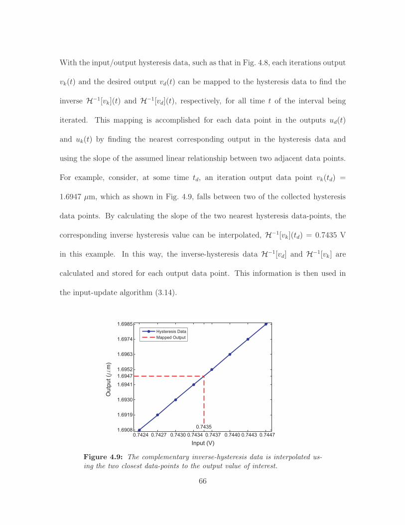
With the input/output hysteresis data, such as that in Fig. 4.8, each iterations output
vk(t) and the desired output vd(t) can be mapped to the hysteresis data to find the
inverse H−1[vk](t) and H−1[vd](t), respectively, for all time t of the interval being
iterated. This mapping is accomplished for each data point in the outputs ud(t)
and uk(t) by finding the nearest corresponding output in the hysteresis data and
using the slope of the assumed linear relationship between two adjacent data points.
For example, consider, at some time td, an iteration output data point vk(td) =
1.6947 µm, which as shown in Fig. 4.9, falls between two of the collected hysteresis
data points. By calculating the slope of the two nearest hysteresis data-points, the
corresponding inverse hysteresis value can be interpolated, H−1[vk](td) = 0.7435 V
in this example. In this way, the inverse-hysteresis data H−1[vd] and H−1[vk] are
calculated and stored for each output data point. This information is then used in
the input-update algorithm (3.14).
0.7424 0.7427 0.7430 0.7434
0.7435
0.7437 0.7440 0.7443 0.74471.6908
1.6919
1.6930
1.6941
1.6947
1.6952
1.6963
1.6974
1.6985
Ou
tpu
t (m
m)
Input (V)
Hysteresis Data
Mapped Output
Figure 4.9: The complementary inverse-hysteresis data is interpolated us-ing the two closest data-points to the output value of interest.
66

4.2.4 Initializing The System
It is an assumption of iterative control that each iteration begins with the same initial
conditions. Therefore, before each iteration k, the initial conditions must be reset to
ensure that each iteration has the same memory of past input. In order to accomplish
this reset, a sinusoidal input is applied, such as that which appears in Fig 4.10. To
clear the memory of the previous iteration, it is necessary that the resetting input
have extrema of the maximum and minimum possible input. With the MI PicoPlus
and data acquisition experimental systems used in this thesis, the maximum input is
±5 V.
0 4 8 12 16 20 24
5
0
5
Time (sec)
Inp
ut
(V)
Figure 4.10: The signal input before each iteration to reset the past-inputmemory of the piezoactuator to the same initial condition.
4.2.5 Executing the Iterative Control Algorithm
With the general desired trajectory partitioned into monotonic sections, the hysteresis
data gathered, and the initial conditions reset, the ICA can truly begin.
67

The input uk is applied and the measured output vk is recorded. This data
is stored in a data file for future analysis. An initial input u1 can be as simple as
u1(t) = 0 for all t in the finite interval T . Alternatively, the initial input u1 can be
designed to give the iteration process a head start, i.e., u1(t) can be a scaled version
of vd(t), but monotonicity of input and output must be maintained.
After each iteration input uk(t) is applied, it is then determined if the output
tracking error ek(t) = vd(t) − vk(t) is less than the predefined acceptable error ε for
all t ∈ T . If the error is within the acceptable range, then the process is complete. If
not, the inverse-hysteresis data collected previously is used to calculate the H−1[uk](t)
for all t ∈ T , the next iterations’ input is calculated using ICA (3.14), the iteration
number k is incremented, the system is reset to the initial state, and the ICA is
repeated.
With the tracking error within the acceptable range, if this is the final mono-
tonic section n ≥ N , the entire process is complete. If n < N , then the entire process
begins again for the next monotonic section by applying the input found for the pre-
vious monotonic section, ramping to determine the hysteresis data, initializing the
system, and executing the ICA (3.14).
4.3 Summary
In summary, the experimental system is a Molecular Imaging (MI, now part of Agilent
Technologies) PicoPlus AFM with custom inputs and outputs to apply controlling
68

voltages to and read from the measured displacement of the piezoactuator.
A benefit of the experimental implementation of ICA (3.14) is that the system
does not require complex modeling. The inverse hysteresis data (H−1[vd] and H−1[vk])
is experimentally obtained. Thus, the hysteresis modeling is not subject to changes
in parameters, temperature, humidity, etc.
The ICA (3.14) is demonstrated through the fabrication technique of dynam-
ically ploughing a polycarbonate sample surface, and the details of this process were
presented. Also detailed was the process of partitioning a general trajectory into
monotonic sections, gathering the hysteresis data used in ICA (3.14), initializing the
system before each iteration, and calculating the next iteration’s input.
In Chapter 5, the experimental results of applying the proposed iterative con-
trol algorithm to the x- and y- axes of the described experimental AFM are presented
along with AFM images of the fabricated feature.
69

Chapter 5
Experimental Results
One of the first uses of an SPM for fabrication was by McCord and Pease
(1987). They were able to use a scanning tunneling microscope to scratch the surface
of a thin insulating film. This act was one of many to demonstrate the potential to
create devices with micrometer-scale lateral precision. To illustrate the effectiveness
of the inverse-hysteresis iterative control algorithm (ICA), it is applied to a fabrication
process with the AFM – dynamically ploughing a polycarbonate surface. The new,
inverse-hysteresis ICA (3.14) is demonstrated with the fabrication process, and, for
comparison, the proportional, P-type algorithm (3.9) is applied to the piezoactuator
as well. Experimental results, including graphical displays of the maximum error emax
vs. iteration k and AFM images of the fabricated feature, both with and without
hysteresis compensation, are presented.
Note:
In every instance to which it is referred, the maximum tracking error is defined and
calculated as
emax ,max{|vd − vk|}
max{vd} − min{vd}. (5.1)
70

5.1 Hysteresis Without Compensation
Without compensation, the effect of hysteresis in the piezoactuator causes significant
tracking error and distortion of the fabricated feature. Figure 5.1 shows the effects
of hysteresis in the desired and measured outputs, the hysteresis curves of each axis,
and an AFM image of the feature fabricated without hysteresis compensation. The
polycarbonate substrate used was not entirely flat and defects are evident. The
maximum possible tracking error due to hysteresis in the x-axis is 13.48% and 14.51%
in the y-axis over the 10 µm displacement range.
5.2 Hysteresis Modeling
A hysteresis model is identified using the polynomial method described in reference
(Croft and Devasia, 1998) and in Section 2.3. The model is used to compute the itera-
tion gain α of the inverse-hysteresis iterative control algorithm (3.14). The MATLAB
program used to find the polynomial coefficients that fit the input/output data best
in a least-squares sense is presented in the Appendix.
The polynomial found for each monotonic section of the x-axis trajectory and
the associated absolute maximum error between the modeled and the measured out-
puts appear in Table 5.1. The same method is used to calculate a polynomial to fit
the open-loop input/output data of each monotonic section of the y-axis trajectory
and they are also shown in Table 5.1. The polynomial model effectively models the
hysteresis with an accuracy of 2% or better.
71

1.0 2.0 2.9-5
0
5
Time (sec)
Dis
pla
ce
me
nt
(m m
)
Desired
Actual
x
y
0 -5 0 5-5
0
5
x (m m)
y (m
m)
(a) (b)
-1.5 -0.75 0 0.75 1.5
-5
-2.5
0
2.5
5
Input (V)
Dis
pla
ce
me
nt
(m m
)
Desired
Actual
13.48% error
-1.5 -0.75 0 0.75 1.5
-5
-2.5
0
2.5
5
Input (V)
Dis
pla
ce
me
nt
(m m
)
Desired
Actual
14.51% error
(c) (d)
(e)
Figure 5.1: The open-loop, uncompensated performance of the piezoactua-tor: (a) The x and y trajectories versus time, (b) a top view of the fabricationtrajectory, the hysteresis curves of (c) the x- and (d) the y- axes, and (e) anAFM image of the fabricated feature.
72

Table 5.1: Polynomial models of the x- and y-axis trajectories.
MonotonicPolynomial Model
MaximumSection Error
A u(t)3 + B u(t)2 + C u(t) + D
x-axis
1 −0.035 u(t)3 + 0.532 u(t)2 + 2.536 u(t) − 0.006 0.86%
2 0.020 u(t)3 − 0.251 u(t)2 + 3.240 u(t) + 0.648 1.05%
3 0.021 u(t)3 + 0.263 u(t)2 + 3.262 u(t) − 0.645 0.41%
4 0.340 u(t)3 − 1.084 u(t)2 + 3.908 u(t) + 0.515 1.85%
y-axis
1 0.161 u(t)3 − 0.253 u(t)2 + 2.618 u(t) − 0.052 1.40%
2 0.025 u(t)3 + 0.270 u(t)2 + 3.282 u(t) − 0.734 0.52%
3 0.141 u(t)3 − 0.763 u(t)2 + 3.829 u(t) + 0.547 2.00%
5.3 Calculating Iteration Gains α and ρ
A condition of convergence of the inverse-hysteresis ICA (3.14) is that the iteration
gain α is limited per Eq. (3.15) (Ashley et al., 2008). Thus, the coefficients ξ2, ξ1, and
M must be calculated. It is assumed that the difference in the output of the inverse
hysteresis model is bounded such that,
ξ1
(
v2(t2) − v1(t1))m
≤ H−1[v2](t2) −H−1[v1](t1) ≤ ξ2
(
v2(t2) − v1(t1))
, (5.2)
where ξ1 and ξ2 are real constants, u1(t1) ≤ u2(t2) for any t1, t2 ∈ T , the input/output
pairs (u1(t1), v1(t1)) and (u2(t2), v2(t2)) belong to the same continuous, monotonic
73

input/output branch, and where m is a positive integer. Additionally, it is assumed
there exists a constant 0 < M < ∞, such that for every change of input, the output
change is bounded,
εu
(
ek(t))
≤ Mek(t), (5.3)
where the error in input εu(·) is monotonic in the output difference ek and εu(ek(t)) = 0
when ek(t) = 0 for all t ∈ T . These relationships, (5.2) and (5.3), allow the calculation
of the coefficients ξ2, ξ1, and M . It is noted that in order to consider the most
conservative iteration gain α, the minimum value of the constant ξ1 and the maximum
values of ξ2 and M are considered.
Based on the input bounding Eq. (5.2), the constant ξ2 can be calculated
ξ2 ≥H−1[v2](t2) −H−1[v1](t1)
v2(t2) − v1(t1). (5.4)
Using a polynomial hysteresis model of the type and order of Eq. (2.1) (and shown
in Table 5.1) and assuming the polynomial perfectly models the hysteresis, that is,
H−1[v](t) = u(t), the constant ξ2 can be represented,
ξ2≥H−1[v2](t2) −H−1[v1](t1)
Au2(t2)3 + Bu2(t2)2 + Cu2(t2) + D − Au1(t1)3 − Bu1(t1)2 − Cu1(t1) − D,
ξ2≥u2(t2) − u1(t1)
A(u2(t2)3 − u1(t1)3) + B(u2(t2)2 − u1(t1)2) + C(u2(t2) − u1(t1)),
ξ2≥1
A(u2(t2)2 + u2(t2)u1(t1) + u1(t1)2) + B(u2(t2) + u1(t1)) + C, (5.5)
74

where A, B, C, and D are the polynomial coefficients of Eq. (2.1). Similarly, based
on Eq. (5.2), the constant ξ1 can be calculated as
ξ1≤(H−1[v2](t2) −H−1[v1](t1))
(
A(u2(t2)3 − u1(t1)3) + B(u2(t2)2 − u1(t1)2) + C(u2(t2) − u1(t1)))m .
Because higher orders of m produce larger values of ξ1, m is set to equal 1. Assuming
a perfect hysteresis model,
ξ1≤1
A(u2(t2)2 + u2(t2)u1(t1) + u1(t1)2) + B(u2(t2) + u1(t1)) + C, (5.6)
again where A, B, and C, are the polynomial coefficients of Eq. (2.1).
Based on the output change bounding Eq. (5.3), the constant M is calculated
as a maximum of the inverse of the slope of the input/output curve. It is noted that
because the individual monotonic sections may not contain the smallest input/output
slope, and therefore, the largest M , the constant α is calculated by using two times
the M computed for each monotonic section.
Using these methods, the constants ξ1, ξ2, M , and α are calculated for each
monotonic section of the x- and y- axes and shown in Tables 5.2 and 5.3, respectively.
From the calculations, the values α = 0.05, α = 0.10, and α = 0.50 were chosen to
determine the effect of α on the performance of the inverse-hysteresis ICA (3.14).
Similarly, in the work of Leang and Devasia (2006) it is proven that conver-
gence of the proportional ICA (3.9) is guaranteed if the iteration gain ρ is limited per
75

Table 5.2: The constants ξ1, ξ2, M , and α as calculated for the x-axistrajectory.
Monotonic Section ξ1 ξ2 M α
1 0.2689 0.4244 0.1514 0.4671
2 0.2421 0.3808 0.0380 0.5780
3 0.2385 0.3823 0.0380 0.5674
4 0.2559 0.3631 0.1514 0.4974
Table 5.3: The constants ξ1, ξ2, M , and α as calculated for the y-axistrajectory.
Monotonic Section ξ1 ξ2 M α
1 0.2239 0.3819 0.0347 0.5375
2 0.2345 0.3781 0.0347 0.5681
3 0.2612 0.4010 0.0347 0.5994
Eq. (3.10). The Preisach hysteresis model is used to determine an appropriate itera-
tion gain ρ for convergence of the P-type ICA (3.9), and is calculated 0 < ρ ≤ 0.062.
Details of this calculation are presented in reference (Ashley et al., 2008). In exper-
iments using the P-type ICA, the value ρ = 0.05 is used, which is within the range
calculated.
5.4 Application of Iterative Control
In this section, the iterative control method is applied to the x- and y- axes of the
piezoactuator of the experimental Molecular Imaging PicoPlus AFM described in
76
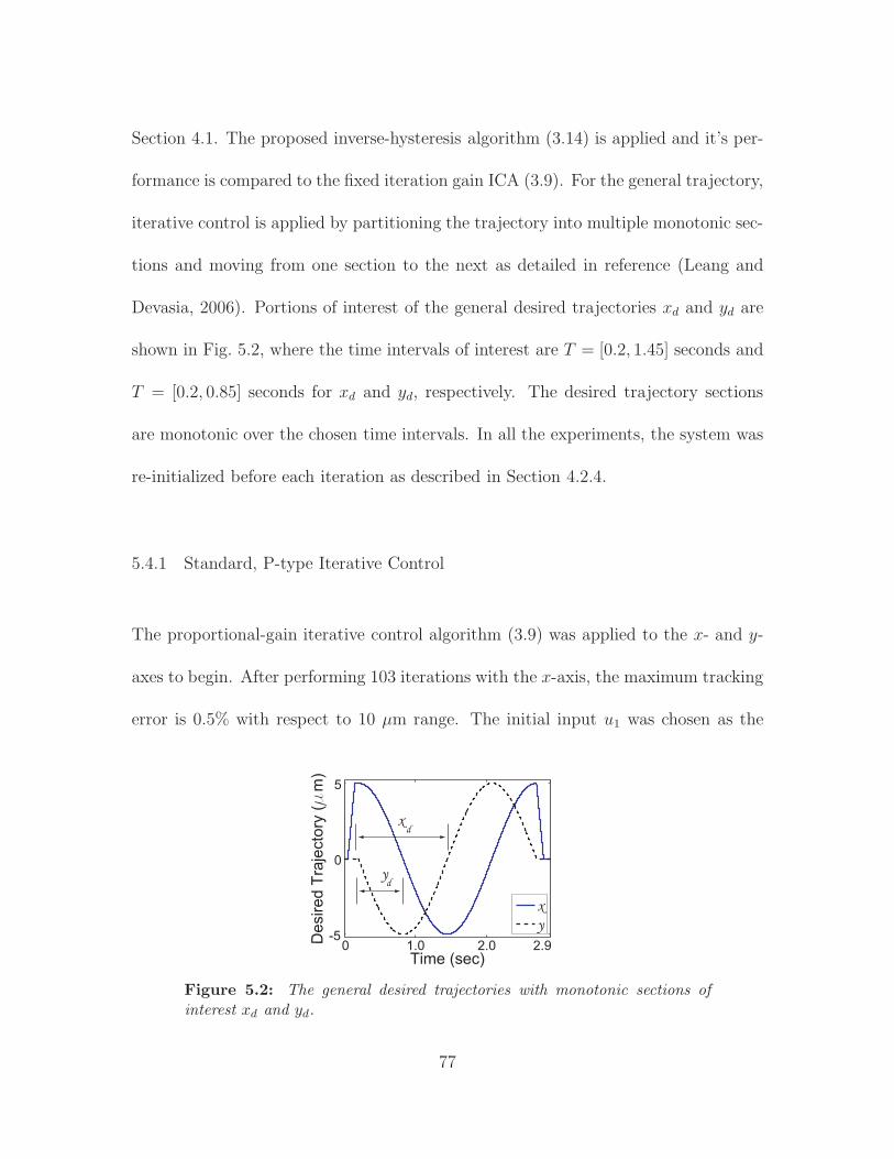
Section 4.1. The proposed inverse-hysteresis algorithm (3.14) is applied and it’s per-
formance is compared to the fixed iteration gain ICA (3.9). For the general trajectory,
iterative control is applied by partitioning the trajectory into multiple monotonic sec-
tions and moving from one section to the next as detailed in reference (Leang and
Devasia, 2006). Portions of interest of the general desired trajectories xd and yd are
shown in Fig. 5.2, where the time intervals of interest are T = [0.2, 1.45] seconds and
T = [0.2, 0.85] seconds for xd and yd, respectively. The desired trajectory sections
are monotonic over the chosen time intervals. In all the experiments, the system was
re-initialized before each iteration as described in Section 4.2.4.
5.4.1 Standard, P-type Iterative Control
The proportional-gain iterative control algorithm (3.9) was applied to the x- and y-
axes to begin. After performing 103 iterations with the x-axis, the maximum tracking
error is 0.5% with respect to 10 µm range. The initial input u1 was chosen as the
0 1.0 2.0 2.9-5
0
5
Time (sec)
Desire
d T
raje
cto
ry (
mm
)
x
y
xd
yd
Figure 5.2: The general desired trajectories with monotonic sections ofinterest xd and yd.
77

desired trajectory scaled by a constant value to give the iteration process a head
start. The tracking results are shown in Fig. 5.3 as well as the maximum error versus
iteration step k.
The constant-gain ICA (3.9) was applied to the y-axis as well. The tracking
results of several iterations and the maximum error emax versus iteration k are shown
in Fig. 5.4. The y-axis requires several more iterations to achieve less than 1% error
over the displacement range because the x-axis input for iteration k = 1 gives the
process a head-start.
5.4.2 Inverse-Hysteresis Iterative Control
The inverse-hysteresis-based iterative control input-update law (3.14) was applied
using the same desired trajectory xd. The value of α was 0.05, 0.1, and 0.5 to better
understand the effect of α on the performance of the algorithm. By incorporating the
0.2 0.4 0.6 0.8 1 1.2 1.4−5
−2.5
0
2.5
5
Vk (
µm
)
Time (sec)
k = 1
k = 10
k = 20
k = 60
k = 121
xd
20 40 60 80 100 1200
20
40
60
Iteration number, k
Err
or
MA
X (
%)
0.17%
ρ = 0.05
(a) (b)
Figure 5.3: Results of proportional iterative control (ρ = 0.05) applied tothe x-axis. The output (a) for several particular trials and (b) the magnitudeof maximum tracking error for each iteration k.
78

0.2 0.4 0.6 0.8
-5
-4
-3
-2
-1
0V
(m
m)
Time (sec)
k = 1
k = 10
k = 20
k = 125
k = 60yd
k
20 40 60 80 100 120 1400
20
40
60
80
100
Iteration number, k
Err
or M
AX (
%)
r=0.05
0.36%
(a) (b)
Figure 5.4: Experimental results of iterative control with constant iterationgain (ρ = 0.05) as applied to the y-axis: (a) The output for several trials;(b) The magnitude of maximum tracking error versus iteration k.
experimental inverse-hysteresis model, ICA (3.14) converges more rapidly than the
proportional ICA (3.9). The tracking results of inverse-hysteresis iterative control as
applied to the x-axis at different iteration steps are shown in Fig. 5.5(a) as well as
the magnitude of the maximum error versus iteration step k shown in Fig. 5.5(b).
Based on the success of using an iteration gain α = 0.5 when ICA (3.14) was
applied to the x-axis, only the value α = 0.5 was used in the y-axis. Several iterations
of inverse-hysteresis iterative control as applied to the y-axis are shown in Fig. 5.5(c),
and the maximum error versus iteration k is shown in Fig. 5.5(d). With α = 0.5, after
9 iterations the maximum error of the inverse-based ICA converges to 0.5% in the
x-axis, while the y-axis requires 21 iterations to achieve 0.5%. This difference in the
number of iterations required is, again, because of the head-start the x-axis is given.
Figure 5.5(e) shows the fabrication results using the inverse-hysteresis ICA (3.14),
and the desired circular feature the inverse-hysteresis algorithm achieved.
79

0.4 0.6 0.8 1 1.2 1.4-5
-3
0
3
5
Outp
ut m
m)
Time (sec)
k = 1
k = 2
k = 3
k = 5k = 8
vd
20 40 60 80 100 1200
10
20
30
40
50
Iteration number, k
Err
or m
ax (
%)
a = 0.50
a = 0.10
a = 0.05
0.358%
0.176%0.051%
(a) (c)
0.2 0.4 0.6 0.8
-5
-4
-3
-2
-1
0
Outp
ut m
m)
Time (sec)
k = 1
k = 3
k = 5
k = 9
k = 16
vd
5 10 15 20 250
20
40
60
80
Iteration number, k
Err
or m
ax (
%)
a = 0.5
0.225%
(b) (d)
(e)
Figure 5.5: Several iterations of the inverse-hysteresis ICA (α = 0.5) asapplied to (a) the x-axis and (b) the y-axis. The maximum error vs. iterationk as applied to (c) the x-axis and (d) the y-axis. An AFM image (e) of thefabricated feature with inverse-hysteresis iterative control applied.
80

5.5 Comparative Results
In order to demonstrate the effectiveness of the inverse-hysteresis ICA (3.14), it and
the proportional ICA (3.9) were both applied to the same desired trajectories – xd
and yd as they appear in Fig. 5.2. As can be seen in Table 5.4, the inverse-hysteresis
algorithm (α = 0.5) requires many fewer iterations than the proportional iterative
control to achieve the same level of precision. The improvement in the rate of conver-
gence is nearly ten-fold compared to the constant iteration gain approach. As seen in
Table 5.4, the inverse-hysteresis algorithm, as applied to the y-axis, requires only 15
iterations to reduce the maximum error from 16% to 0.25%, while the proportional
ICA requires more than 100 iterations.
Table 5.4: Comparison of number of iterations to achieve various levelsof maximum error for the proportional P-type and inverse-hysteresis H−1
iterative control algorithms.
x-axis y-axisP-type H−1 Maximum H−1 P-type
ρ = 0.05 α = 0.5 Error α = 0.5 ρ = 0.05
29 3 16.0% 8 50
59 6 4.0% 13 84
80 7 1.5% 16 110
89 8 1.0% 18 123
103 9 0.5% 21 146
121 11 0.25% 23More Than
150†
†In 150 iterations a maximum error of 0.36% is achieved.
81

This improvement relates to real time savings waiting for the iterative process
to be completed. In these experiments, each iteration required more than one minute
to complete, thus, 110 or 130 fewer iterations to achieve 0.25% error means real time
savings. This time-savings opens the door for iterative control to be considered a
production-level control technique for SPM-based nano-fabrication.
As shown in Fig. 5.5(b), the performance of the inverse-hysteresis ICA (3.14) is
improved by increasing the value of the iteration gain α. Based on the calculations in
Tables 5.2 and 5.3, the gain α could be further increased for some monotonic sections,
thus, improving the performance of inverse-hysteresis iterative control even further.
82

Chapter 6
Conclusions
In conclusion, this thesis investigated the iterative control method used to
compensate for hysteresis effect in the piezoactuators of atomic force microscopy.
The details of how the atomic force microscope came to be invented, along
with an investigation of the modes and components of operation, were presented.
The piezoactuator is commonly used to move the AFM-probe tip relative to the
sample surface, partially because of the possibility of atomic-resolution positioning.
Unfortunately, the piezoactuators motion is negatively impacted by the effects of
hysteresis (as well as creep and vibration).
Hysteresis is a complex, nonlinear effect observed between the applied input
and the output of the system. The previous attempts to compensate for hystere-
sis, including feedback and inverse model-based feed-forward control, were discussed.
While there are advantages to feedback and inversion-based feed-forward methods,
they are overshadowed by the inherent low gain-margin of the piezoactuator and the
computational complexity of modeling a system prone to change. The previous work
toward iterative control of hysteresis and the motivation to achieve precision control
in fewer iterations than previously possible were also described.
83

The proposed iterative control algorithm (3.14) incorporates an approximate,
experimentally-calculated inverse hysteresis model, and, therefore, does not require
complex modeling unlike other model inversion-based control techniques. The condi-
tions for convergence of the inverse-hysteresis ICA were presented to achieve precision
control along a single hysteresis branch. The inverse-hysteresis ICA and proportional
iterative control were both applied to the same desired trajectories, and results were
presented for the same monotonic sections of the desired trajectory, xd and yd, to
demonstrate the effectiveness of the new iterative control algorithm. The method to
find an input which achieves a general, multi-branch desired trajectory was exploited
to achieve the circular motion of the piezoactuator in the x/y plane.
The inverse-hysteresis ICA was able to achieve a trajectory which is within
0.225% of the desired trajectory over the displacement range. This error equates to
±22.5 nm = ±5.57 mV from the inductive position sensors, which is approaching the
resolution of the experimental data acquisition system at ±2.4 mV.
The experimental results show that the inverse-hysteresis ICA offers conver-
gence in fewer iterations compared to other hysteresis-compensating iterative algo-
rithms. It is specifically shown that compared to the standard, proportional ICA,
the inverse-hysteresis model-based iterative algorithm offers a ten-fold improved rate
of convergence. The inverse-hysteresis ICA is able to reduce the maximum error in
the x-axis from 16% to 0.25% in 8 iterations, while the proportional ICA requires
92 iterations. This improvement relates to real time savings waiting for the iterative
84

process to be completed.
The new iterative control method was applied to fabricate a five-micron radius
circular feature with better than 25 nm precision using the experimental AFM to
demonstrate the capability and effectiveness of the inverse-hysteresis iterative control
approach in micro-fabrication. The success of the inverse-hysteresis ICA shows that
iterative control can be a viable production-level control scheme and can be used in
the SPM-based mass production of emergent nano-technologies – a trajectory can
now be “learned” in minutes as opposed to the hours it took previously.
85

Chapter 7
Future Work
While the experimental results of the proposed inverse-hysteresis iterative con-
trol algorithm (3.14) have shown one magnitude of improvement in the number of
iterations required to reach a minimal error in the hysteretic AFM system, there are
several key aspects that warrant further investigation.
An opportunity for exploration is combining the inverse-hysteresis ICA with
inverse vibration and inverse creep models to be able to compensate for the hysteresis
and dynamic effects. The hysteresis, vibration, and creep effects have been modeled
as a cascade of a nonlinear hysteresis and a linear, time-invariant (LTI) dynamic block
as shown in Fig. 7.1 (Croft et al., 2001). As such, the dynamic effects can be modeled
and an inverse model can then be used to find an appropriate input ud which achieves
a desired output yd with each of the hysteresis, vibration, and creep effects accounted
for and compensated. Such compensation would allow for trajectories to operate at
high frequencies with high precision.
H LTI
Piezoactuator
u v y
Figure 7.1: Cascade model of a piezoactuator.
86

Additionally, the iterative control algorithm developed in this thesis was used
to compensate for the effects of hysteresis in the piezoactuator of AFM. The algorithm
has potential uses in a variety of other applications. Shape memory alloys (SMA) have
been used in novel cell and tissue stretching devices (Shan et al., 2007). Unfortunately,
the precision performance of SMA is severely compromised by the effects of hysteresis
(Gorbet et al., 1998). The standard, P-type iterative method was applied to SMA
(Leang et al., 2009a), but required more than 500 iterations to achieve better than 20%
error over the displacement range. Iterative control has been applied to other systems
which exhibit hysteresis, such as electromagnetic actuators (Tseng et al., 2008). The
inverse-hysteresis ICA developed in this work may offer improved performance when
applied to these and other hysteretic systems.
87

List of References
88

List of References
Agilent Technologies. Closed-loop Scanner Datasheet, #PF 010 SCAN 9-04-5000,
2004.
H.-S. Ahn, K. L. Moore, and Y. Chen. Iterative Learning Control: Robustness and
Monotonic Convergence for Interval Systems. Springer-Verlag, London, 2007.
T. R. Albrecht and C. F. Quate. Atomic resolution imaging of a nonconductor by
atomic force microscopy. J, Appl. Phys., 62(7):2599–2602, 1 Oct. 1987.
T. R. Albrecht, P. Grutter, D. Horne, and D. Rugar. Frequency modulation detection
using high-Q cantilevers for enhanced force microscope sensitivity. J. Appl.
Phys., 69:668–673, 1991.
R. M. Allen. The Microscope. D. Van Nostrand Company, Inc., New York, 1940.
D. P. Allison, P. S. Kerper, M. J. Doktycz, J. A. Spain, P. Modrich, F. W. Larimer,
T. Thundat, and R. J. Warmack. Direct atomic force microscope imaging of
EcoRI endonuclease site specifically bound to plasmid DNA molecules. Proc.
Natl. Acad. Sci. USA, 93:8826–8829, 1996.
M. A. Alsubaie, Z. Cai, C. T. Freeman, P. L. Lewin, and E. Rogers. Repetitive and
iterative learning controllers designed by duality with experimental verification.
In Proc. 17th IFAC World Congress, pages 3562–3567, Seoul, Korea, 2008.
G. Apetrii, S. F. Fischer, U. Kunze, D. Reuter, and A. D. Wieck. Influence of
processing parameters on the transport properties of quantum point contacts
fabricated with an atomic force microscope. Semicond. Sci. Technol., 17:735–
739, 2002.
S. Arimoto, S. Kawamura, and F. Miyazaki. Bettering operation of robots by learning.
J. Robot. Syst., 1(2):123–140, 1984.
89
S. C. Ashley, G. Tchoupo, R. M. Mohr, and K. K. Leang. Precise positioning of a
shape memory alloy actuator using iterative control. In Proc. Actuator 2006
Conf., Bremen, Germany, 14 June 2006.
S. C. Ashley, U. Aridogan, R. Riddle, and K. K. Leang. Hysteresis inverse iterative
learning control of piezoactuators in AFM. In Proc. 17th IFAC World Congress,
pages 8269–8274, Seoul, Korea, 6 July 2008.
R. C. Barrett and C. F. Quate. Optical scan-correction system applied to atomic
force microscopy. Rev. Sci. Instrum., 62(6):1393–1399, 1991.
S. P. Beaumont. III-V Nanoelectronics. Microelectron. Eng., 32:283–295, 1996.
B. Bhushan and N. Chen. AFM studies of environmental effects on nanomechanical
properties and cellular structure of human hair. Ultramicroscopy, 106(8-9):755–
764, 2006.
G. Binnig. Force microscopy. Ultramicroscopy, 42-44:7–15, 1992.
G. Binnig, H. Rohrer, Ch. Gerber, and E. Weibel. Surface studies by scanning tun-
neling microscopy. Phys. Rev. Lett., 49(1):57–61, 1982.
G. Binnig, C. F. Quate, and Ch. Gerber. Atomic force microscope. Phys. Rev. Lett.,
56(9):930–933, 1986.
B. Boulet. Introduction to feedback control systems. Technical report, Coronado
Systems, April 2000.
Z. Cai, C. Freeman, E. Rogers, and P. Lewin. Reference shift iterative learning control
for a non-minimum phase plant. In Proc. Am. Control Conf., pages 558–563,
New York, NY, 9 July 2007.
V. Cambel, J. Martaus, J. Soltys, R. Kudela, and D. Grgusova. Local anodic oxidation
by AFM tip developed for novel semiconductor nanodevices. Ultramicroscopy,
108:1021–1024, 2008.
Y. Chen and K. L. Moore. Comments on United States Patent 3,555,252 – “Learn-
ing control of actuators in control systems”. In Proc. Intl. Conf. Automation,
Robotics, and Control, Singapore, 2000.
90

J.-W. Choi, H.-G. Choi, K.-S. Lee, and W.-H. Lee. Control of ethanol concentration
in a fed-batch cultivation of acinetobacter calcoaceticus RAG-1 using a feedback-
assisted iterative learning algorithm. J. Biotechnol., 49(1-3):29–43, Aug. 1996.
G. M. Clayton, S. Tien, K. K. Leang, Q. Zou, and S. Devasia. A review of feed-
forward control approaches in nanopositioning for high speed SPM. ASME J.
Dyn. Syst. Meas. and Cont., Special Issue on Dynamic Modeling, Control, and
Manipulation at the Nanoscale, 131(6):061101 (19 pages), 2009.
D. Croft and S. Devasia. Hysteresis and vibration compensation for piezoactuators.
J. Guid. Control Dyn., 21(5):710–717, Sept. 1998.
D. Croft, G. Shed, and S. Devasia. Creep, hysteresis, and vibration compensation
for piezoactuators: Atomic force microscopy application. Trans. ASME J. Dyn.
Syst. Meas. Control, 123:35–43, 2001.
R. Cross, M. Grinfeld, and H. Lamba. Hysteresis and economics. IEEE Control Syst.
Mag., 29(1):30–43, Feb. 2009.
A. Daniele, S. Salapaka, M. V. Salapaka, and M. Dahleh. Piezoelectric scanners for
atomic force microscopes: Design of lateral sensors, identification and control.
In Proc. Am. Control Conf., pages 253–257, San Diego, CA, June 1999.
Z. J. Davis, G. Abadal, O. Kuhn, O. Hansen, F. Grey, and A. Boisen. Fabrication
and characterixation of nanoresonating devices for mass detection. J. Vac. Sci.
Technol. B, Microelectron. Nanometer Struct., 18(2):612–615, 2000.
S. Decossas, F. Mazen, T. Baron, G. Bremond, and A. Souifi. Atomic force mi-
croscopy nanomanipulation of silicon nanocrystals for nanodevice fabrication.
Nanotechnol., 14:1272–1278, 2003.
B. Delibas, A. Arockiarajan, and W. Seemann. Nonlinear simulation of piezoceramic
material using micromechanical approach. In Proc. Struct., Struct. Dyn., and
Mater. Conf., volume 4, pages 3245–3253, Palm Springs, CA, 19 April 2004.
S. Devasia. Robust inversion-based feedforward controllers for output tracking un-
der plant uncertainty. In Proc. Am. Control Conf., volume 1, pages 497–502,
Chicago, IL, 28 June 2000.
91

S. Devasia, E. Eleftheriou, and S. O. R. Moheimani. A survey of control issues in
nanopositioning. IEEE Trans. Contr. Syst. Technol., 15(5):802–823, 2007.
M. O. Donnagain. Semi-linear duffing equation with discrete preisach nonlinearity.
Master’s thesis, National University of Ireland, Cork, Oct. 2004.
H. Dou, Z. Zhou, M. Sun, and Y. Chen. Robust high-order P-type iterative learning
control for a class of uncertain nonlinear systems. In Intl. Conf. Syst., Man and
Cybernetics, volume 2, pages 923–928, New York, NY, 14 Oct. 1996.
C. C. Doumanidis. Nano-manufacturing: Technical advances, research challenges and
future directions. Proc. Inst. Mech. Eng. N, J. Nanoeng. Nanosyst., 218(N2):
51–70, 2004.
O. M. El Rifai, B. D. Aumond, and K. Youcef-Toumi. Imaging at the nano-scale. In
Proc. of IEEE/ASME Intl. Conf. Advanced Intell. Mechatron., volume 2, pages
715–722, Port Island, Kobe, Japan, 20 July 2003.
R. Erlandsson, G. M. McClelland, C. M. Mate, and S. Chiang. Atomic force mi-
croscopy using optical interferometry. J. Vac. Sci. Technol. Part A Vac. Surf.
Films, 6(2):266–270, 1988.
L. Fan and Y. Liu. Iterative learning control for linear motor motion system. In Proc.
IEEE Intl. Conf. Automat. and Logis., pages 2379–2383, Aug. 2007.
A. J. Fleming and A. G. Wills. Optimal periodic trajectories for band-limited systems.
IEEE Control Syst. Technol., 13(3):552–562, 2009.
C. Freeman, P. L. Lewin, and E. Rogers. Further results on the experimental eval-
uation of iterative learning control algorithms for non-minimum phase plants.
Intl. J. Control, 80(4):569–582, April 2007.
C. T. Freeman, A.-M. Hughes, J. H. Burridge, P. H. Chappell, P. L. Lewin, and
E. Rogers. Iterative learning control of FES applied to the upper extremity for
rehabilitation. Control Eng. Prac., 17(3):368–381, March 2009.
M. Garden. US Patent #3555252, Learning control of actuators in control systems,
Filed: 11 May, 1967.
92

P. Ge and M. Jouaneh. Modeling hysteresis in piezoceramic actuators. Precision
Eng., 17(3):211–221, 1995.
F. J. Giessibl. Atomic resolution of the silicon (111)-(7 × 7) surface by atomic force
microscopy. Science, 267:68–71, 1995.
F. J. Giessibl. Advances in atomic force microscopy. Rev. Modern Phys., 75(3):
949–983, 2003.
F. J. Goforth and Z. Gao. An active disturbance rejection control solution for hys-
teresis compensation. In Proc. Am. Control Conf., pages 2202–2208, Seattle,
WA, 11 June 2008.
M. Goldfarb and N. Celanovic. Modeling piezoelectric stack actuators for control of
micromanipulation. IEEE Control Syst. Mag., 17(3):69–79, June 1997.
R. B. Gorbet, D. W. L. Wang, and K. A. Morris. Preisach model identification of a
two-wire SMA actuator. In Proc. IEEE Conf. on Robotics & Automat., volume 3,
pages 2161–2167, Leuven, Belgium, 16 May 1998.
A. J. Hughes Hallett and L. Piscitelli. Testing for hysteresis against nonlinear alter-
natives. J. Econ. Dyn. & Control, 27:303–327, 2002.
K. Hamaya, M. Kitabatake, K. Shibata, M. Jung, M. Kawamura, K. Hirakawa,
T. Machida, T. Taniyama, S. Ishida, and Y. Arakawa. Electric-field control
of tunneling magnetoresistance effect in a Ni/InAs/Ni quantum-dot spin valve.
Appl. Phys. Lett., 91(2):22107 (3 pages), 9 July 2007.
X. Hao, L. Zhang, and H. Li. A new PD type iterative learning control in active control
for vibration. In Proc. Intell. Control Automat., pages 922–926, Chongqing,
China, 25 June 2008.
T. Hegewald, B. Kaltenbacher, M. Kaltenbacher, and R. Lerch. Efficient modeling of
ferroelectric behavior for the analysis of piezoceramic actuators. J. Intel. Mater.
Syst. Struct., 19:1117–1129, Oct. 2008.
B. E. Helfrich, C. Lee, D. A. Bristow, X. H. Xiao, J. Dong, A. G. Alleyne, S. M.
Salapaka, and P. M. Ferreira. Combined H∞-feedback and iterative learning
control design with application to nanopositioning systems. In Proc. Am. Control
Conf., pages 3893–3900, Seattle, WA, 11 June 2008.
93
K. J. G. Hinnen, R. Fraanje, and M. Verhaegen. The application of initial state
correction in iterative learning control and the experimental validation on a
piezoelectric tube scanner. Proc. of the Inst. Mech. Engineers. Part I: J. Syst.
and Control Engr., 218(6):503–511, Sept. 2004.
H. Hoelzle, A. G. Alleyne, and A. J. W. Johnson. Iterative learning control for robotic
deposition using machine vision. In Proc. Am. Control Conf., pages 4541–4547,
Seattle, WA, 11 June 2008.
A. E. Holman, P. M. L. O. Scholte, W. Chr. Heerens, and F. Tuinstra. Analysis
of piezo actuators in translation constructions. Rev. Sci. Instrum., 66(5):3208–
3215, May 1995.
R. Hooke. Micrographia, or Some Physiological Desciptions of Minute Bodies. Cosimo
Classics, from original 1665 version, New York, 2007.
H. Hu and R. B. Mrad. On the classical Preisach model for hysteresis in piezoceramic
actuators. Mechatronics, 13(2):85–94, March 2003.
M. Hu, H. Du, S.-F. Ling, Z. Zhou, and Y. Li. Motion control of an electrostrictive
actuator. Mechatronics, 14:153–161, March 2004.
T. Hu, D. Wang, L. Shen, Y. Sun, and H. Wang. Iterative learning control for a class
of systems with hysteresis. In Proc. Intl. Conf. Control, Automat., Robotics,
and Vision, pages 10–15, Hanoi, Vietnam, 17 Dec. 2008.
S. M. Hues, C. F. Draper, K. P. Lee, and R. J. Colton. Effect of PZT actuator
hysteresis and creep on nanoindentation measurements using force microscopy.
Rev. Sci. Instrum., 65(5):1561–1565, May 1994.
D. Hughes and J. T. Wen. Preisach modeling of piezoceramic and shape memory
alloy hysteresis. Smart Mater. Struct., 6(3):287–300, June 1997.
R. Huxley, editor. The Great Naturalists. Thames & Hudson, New York, 2007.
M. Hwang, M. Farhoud, Y. Hao, M. Walsh, T. A. Savas, H. I. Smith, and C. A.
Ross. Major hysteresis loop modeling of two-dimensional arrays of single domain
particles. IEEE Trans. Magn., 36(5):3173–3175, Sept. 2000.
94

R. V. Iyer, X. Tan, and P. S. Krishnaprasad. Approximate inversion of the preisach
hysteresis operator with application to control of smart actuators. IEEE Trans.
Autom. Control, 50(6):798–810, 2005.
B. Jaffe, W. R. Cook, and H. Jaffe. Piezoelectric Ceramics. Academic Press, London,
1971.
D. C. Jiles and D. L. Atherton. Theory of ferromagnetic hysteresis (invited). J. Appl.
Phys., 55:2115–2120, Mar. 1984.
M. Jung, K. Hirakawa, Y. Kawaguchi, S. Komiyama, S. Ishida, and Y. Arakawa.
Lateral electron transport through single self-assembled InAs quantum dots.
Appl. Phys. Lett., 86(3):1–3, 17 Jan. 2005.
S.-B. Jung and S.-W. Kim. Improvement of scanning accuracy of PZT piezoelectric
actuators by feed-forward model-reference control. Prec. Engr., 16(1):49–55,
Jan. 1994.
H. Kaizuka. Application of capacitor insertion method to scanning tunneling micro-
scopes. Rev. Sci. Instrum., 60(10):3119–3122, 1989.
S. Kawamura, F. Miyazaki, and S. Arimoto. Iterative learning control for robot
systems. In Proc. Intl. Conf. Indust. Elec., Control and Instrum., Tokyo, Japan,
22 October 1984.
S. Ko and S.-J. Kim. Transistor characteristics of a parallel-channel and a serial-
channel superconducting flux flow transistor fabricated by the AFM anodization
process. Curr. Appl. Phys., 9(1):S35–S37, Jan 2009.
T. F. Krauss. Control at the quantum level. Science, 308:1122–1123, 2005.
U. Kunze. Invited Review: Nanoscale devices fabricated by dynamic ploughing with
an atomic force microscope. Supperlattices and Microstruct., 31(1):3–17, 2002.
K. K. Leang and S. Devasia. Design of hysteresis-compensating iterative learning
control for piezo-positioners: Application to atomic force microscopes. Mecha-
tronics, 16(3-4):141–158, 2006.
95

K. K. Leang and S. Devasia. Feedback-linearized inverse feedforward for creep, hys-
teresis, and vibration compensation in AFM piezoactuators. IEEE Trans. Contr.
Syst. Technol., 15(5):927–935, 2007.
K. K. Leang, S. C. Ashley, and G. Tchoupo. Iterative and feedback control for
hysteresis compensation in SMA. Trans. ASME J. Dyn. Syst. Meas. Control,
131(1):14502 (6 pages), Jan. 2009a.
K. K. Leang, Q. Zou, and S. Devasia. Feedforward control of piezoactuators in
atomic force microscope systems: Inversion-based compensation for dynamics
and hysteresis. IEEE Cont. Syst. Mag., Special Issue on Hysteresis, 29(1):70–
82, Feb. 2009b.
D. Leonard, M. Krishnamurthy, C. M. Reaves, S. P. Denbaars, and P. M. Petroff.
Direct formation of quantum-sized dots from uniform coherent islands of InGaAs
on GaAs surfaces. Appl. Phys. Lett., 63(23):3203–3205, 6 Dec. 1993.
L. Li and J. Mao. Feedback linearisation of magnetic bearing actuators for a uniform
upper bound of force slew rate. IEE Proc., Electr. Power Appl., 146(4):378–382,
July 1999.
T. Li, X. Zhang, X. Jiang, Y. Li, and Z. Du. Fabrication of gold nanoelectrodes based
on nanolithography electrochemically through a conductive AFM tip. Chin. Sci.
Bull., 50(22):2560–2564, Nov. 2005.
Z. Li, M. Wu, T. Liu, C. Wu, and B. Zhao. Preparation of TiO2 nanowire gas
nanosensor by AFM anode oxidation. Ultramicroscopy, 108:1334–1337, 2008.
J. A. Lizama. English physicist explains pros of nanotechnology. Richmond Times-
Dispatch, page B2, 21 Oct. 2008.
J. A. Main and E. Garcia. Piezoelectric stack actuators and control system design:
Strategies and pitfalls. J. Guid. Control Dyn., 20(3):479–485, 1997.
J. A. Main, E. Garcia, and D. V. Newton. Precision position control of piezoelectric
actuators using charge feedback. J. Guid. Control Dyn., 18(5):1068–1073, 1995.
P. Mane, K. Mossi, and C. Green. Optimizing energy harvesting parameters using re-
sponse surface methodology. IEEE Trans. Ultrason., Ferroelectr., Freq. Control,
56(3):429–436, March 2009.
96

I. D. Mayergoyz. Hysteresis models from the mathematical and control theory points
of view. J. Appl. Phys., 57(8):3803–3805, April 1985.
I. D. Mayergoyz. Mathematical models of hysteresis. Springer-Verlag, New York,
1991.
O. Mayr. The origins of feedback control. Sci. Amer., 223(4):110–118, 1970.
M. A. McCord and R. F. W. Pease. Scanning tunneling microscope as a microme-
chanical tool. Appl. Phys. Lett., 50(10):569–570, 1987.
E. J. McCumiskey. Mechanical characterization of nanocomposite CdSe quantum
dot - MEH-PPV polymer thin films via nanoindentation. Master’s thesis, Vir-
ginia Commonwealth University, Richmond, Virginia, May 2009.
H. J. McSkimin. Measurement of elastic constants at low temperatures by means of
ultrasonic waves – data for silicon and germanium single crystals, and for fused
silica. J. Appl. Phys., 24(8):988–997, August 1953.
R. V. N. Melnik. Modelling coupled dynamics: Piezoelectric elements under changing
temperature conditions. Intl. Commun. Heat Mass Transf., 30(1):83–92, Jan.
2003.
J. M. Mendel. A survey of learning control systems. ISA Trans., page 297, July 1966.
R. Merry, M. Uyanik, R. van de Molengraft, M. Steinbuch, R. Koops, and M. van
Veghel. Modeling and compensation of asymmetric hysteresis in a piezo actuated
metrological AFM. In Proc. Am. Control Conf., pages 967–972, 10 June 2009.
T. Mita. Repetitive control of mechanical systems. In Proc. ATACS ’84, Izu, Japan,
1984.
B. Mokaberi and A. G. Requicha. Compensation of scanner creep and hysteresis
for AFM nanomanipulation. IEEE Trans. Autom. Sci. and Eng., 5(2):197–206,
2008.
K. L. Moore. Iterative Learning Control for Deterministic Systems. Springer-Verlag,
London, 1993.
97

K. L. Moore. Applied and Computational Control, Signals and Circuits: Volume 1,
chapter Iterative Learning Control – An Expository Overview, pages 151–214.
Birkhauser, Boston, 1999.
K. L. Moore. An introduction to iterative learning control. http://inside.mines.edu/
∼kmoore/ilc-intro-pdftex03-03.pdf, March 2003.
R. Moriya, H. Kobayashi, K. Shibata, S. Masubuchi, K. Hirakawa, S. Ishida,
Y. Arakawa, and T. Machida. Fabrication of single-electron transistor com-
posed of a self-assembled quantum dot and nanogap electrode by atomic force
microscope local oxidation. Appl. Phys. Expr., 3(3):035001 (3 pages), 2010.
A. N. Mucciardi. Elements of learning control systems with applications to industrial
processes. In Proc. IEEE Conf. Decision and Control, pages 320–325, New
Orleans, LA, 13 Dec. 1972.
Y. Murakami, S. Shingubara, H. Sakaue, and T. Takahagi. Formation of aluminum
nano-dot array by the use of nano-indentation and anodic oxidation. In Proc.
Intl. Microproc. and Nanotechnol., pages 166–167, Shimane, Japan, 31 Oct.
2001.
NANOSENSORSTM. PointProbeR© Plus AFM Probes – Product Brochure.
www.nanosensors.com.
C. V. Newcomb and I. Flinn. Improving the linearity of piezoelectric ceramic actua-
tors. Elec. Lett., 18(11):442–444, May 1982.
A. Palevski, C. P. Umbach, and M. Heiblum. High-gain lateral hot-electron device.
Appl. Phys. Lett., 55(14):1421–1423, 1989.
P. Peng, T. Shi, G. Liao, Z. Tang, and C. Liu. Scratch of submicron grooves on
aluminum film with AFM diamond tip. In Proc. IEEE Nano/Micro Engr. Molec.
Syst., pages 983–986, Shenzhen, China, 5 Jan. 2009.
F. Preisach. Uber die magnetische nachwirkung (About the magnetic aftereffect).
Zeitschrift fur Physik, 94(5-6):277–302, May 1935.
A. Preumont. Mechatronics: Dynamics of Electromechanical and Piezoelectric Sys-
tems, volume 136 of Solid Mechanics and its Applications. Springer, Dordrecht,
The Netherlands, 2006.
98

A. S. Putra, S. Huang, K. K. Tan, S. K. Panda, and T. H. Lee. Design, modeling,
and control of piezoelectric actuators for intracytoplasmic sperm injection. IEEE
Trans. Contr. Syst. Technol., 15(5):879–890, 2007.
T. G. Rochow and E. G. Rochow. An Introduction to Microscopy by Means of Light,
Electrons, X-Rays, or Ultrasound. Plenum Press, New York, 1978.
M. Rosenwald. The genius of small things. Smithsonian, 41(4):106–112, July/August
2010.
E. Ruska. The development of the electron microscope and of electron microscopy.
Rev. Mod. Phys., 59(3):627–638, Jul 1987. doi: 10.1103/RevModPhys.59.627.
S. Salapaka, A. Sebastian, J. P. Cleveland, and M. V. Salapaka. High bandwidth
nano-positioner: A robust control approach. Rev. Sci. Instrum., 73(9):3232–
3241, 2002.
D. Sarid, D. Iams, V. Weissenberger, and L. S. Bell. Compact scanning-force micro-
scope using a laser diode. Opt. Lett., 13(12):1057–1059, 1988.
A. Sayir, S. C. Farmer, and F. W. Dynys. High-temperature piezoelectric ceramic
developed. Technical report, Case Western Reserve, Record 57 from NTIS, Jun
2005.
G. Schitter, P. Menold, H. F. Knapp, F. Allgower, and A. Stemmer. High performance
feedback for fast scanning atomic force microscopes. Rev. Sci. Instrum., 72(8):
3320–3327, 2001.
G. Schitter, R. W. Stark, and A. Stemmer. Fast contact-mode atomic force microscopy
on biological specimen by model-based control. Ultramicroscopy, 100:235–257,
2004.
Y. Shan, J. Dodson, S. Abraham, J. E. Speich, R. Rao, and K. K. Leang. A biaxial
shape memory alloy actuated cell/tissue stretching system. In Proc. ASME Intl.
Mech. Eng. Congress and Expo., pages 161–169, Seattle, WA, 11 Nov. 2007.
E. Shimoni. Using AFM to explore food nanostructure. Curr. Opin. Colloid Interface
Sci., 13(5):368–374, Oct. 2008.
99
E. Simion, A. Ceclan, D. D. Micu, L. Cret, and L. Man. Analytical curve fitting of
nonlinear characteristics and hysteresis. In Proc. Symp. Electromagnetic Phen.
Nonlin. Circuits, pages 131–132, Maribor, Slovenia, 28 June 2006.
R. Simkovics, H. Landes, M. Kaltenbacher, and R. Lerch. Finite element analysis
of ferroelectric hysteresis effects in piezoelectric transducers. In Proc. IEEE
Ultrasonics Symp., volume 2, pages 1081–1084, San Juan, Puerto Rico, 22 Oct.
2000.
M. Sirena, S. Fusil, K. Bouzehouane, J.-M. George, and V. Cros. Study of atomic force
microscopy nanoindentation for the developement of nanostructures. Physica B,
404:2705–2709, 2009.
S. Skaberna, M. Versen, B. Klehn, U. Kunze, D. Reuter, and A. D. Wieck. Fabrication
of a quantum point contact by the dynamic plowing technique and wet-chemical
etching. Ultramicroscopy, 82:153–157, 2000.
J. Sklansky. Learning systems for automatic control. IEEE Trans. Autom. Control,
AC-11(1):6–19, Jan. 1966.
R. C. Smith. Inverse compensation for hysteresis in magnetostrictive transducers.
Math. Comput. Model., 33(1-3):285–298, Jan.-Feb. 2001.
R. C. Smith and Z. Ounaies. A domain wall model for hysteresis in piezoelectric
materials. J. Intell. Mater. Syst. Struct., 11(1):62–79, Jan. 2000.
R. C. Smith, M. V. Salapaka, A. Hatch, J. Smith, and T. De. Model development
and inverse compensator design for high speed nanopositioning. In Proc. IEEE
Conf. Decision and Control, pages 3652–3657, Las Vegas, NV, 10 Dec. 2002.
E. S. Snow and P. M. Campbell. Fabrication of Si nanostructures with an atomic
force microscope. Appl. Phys. Lett., 64(15):1932–1934, 1994.
E. S. Snow, P. M. Campbell, and F. K. Perkins. Nanofabrication with proximal
probes. Invted Paper, Proc. IEEE, 85(4):601–611, April 1997.
L. L. Sohn and R. L. Willett. Fabrication of nanostructures using atomic-force-
microscope-based lithography. Appl. Phys. Lett., 67(11):1552–1554, 1995.
100
G. Song, J. Zhao, X. Zhou, and J. A. De Abreu-Garcia. Tracking control of a piezo-
ceramic actuator with hysteresis compensation using inverse preisach model.
IEEE/ASME Trans. Mechatronics, 10(2):198–209, 2005.
Z.-Q. Song, S.-L. Zhou, and X.-J. Shi. Trajectory tracking control for a GMM actuator
based on a heuristic ILC method. Chin. J. Aeronaut., 19:S232–S234, Dec. 2006.
R. Su and N. Kermiche. Learning control for a class of nonlinear systems. In Proc.
IEEE Intl. Symp. Intell. Control, pages 582–585, Albany, NY, 25 Sept. 1989.
T. Sugie and T. Ono. An iterative learning control law for dynamical systems. Au-
tomatica, 27(4):729–732, 1991.
Y. D. Sverkunov. Polynomial approximation of the response of a system with hys-
teresis. Autom. Remote Control, 34(7):1198–1200, July 1973.
N. Tamer and M. Dahleh. Feedback control of piezoelectric tube scanners. In Proc.
IEEE Conf. Decision and Control, pages 1826–1831, Lake Buena Vista, FL, 14
Dec. 1994.
K. K. Tan, K. Y. Chua, S. Zhao, S. Yang, and M. T. Tham. Repetitive control
appraoch towards automatic tuning of Smith predictor controllers. ISA Trans.,
48:16–23, 2009.
G. Tao and P. V. Kokotovic. Adaptive control of systems with actuator and sensor
nonlinearities. Wiley, New York, 1996.
C. R. Taylor, E. A. Stach, A. P. Malshe, and G. Salamo. Analysis of nanoscale
deformation in GaAs(100): Towards patterned growth of quantum dots. In
Proc. Mater. Res. Soc. Symp., volume 864, pages 175–180, San Francisco, CA,
28 March 2005.
S. Tien, Q. Zou, and S. Devasia. Iterative control of dynamics-coupling-caused errors
in piezoscanners during high-speed AFM operation. IEEE Trans. Contr. Syst.
Technol., 13(6):921–931, 2005.
C. Tseng, I. Mayergoyz, P. McAvoy, and C. Krafft. Iterative compensation for hystere-
sis effects in positioning and tracking problems. J. Appl. Phys., 103(7):07D902,
2008.
101

M. Uchiymama. Formation of high speed motion pattern of mechanical arm by trial.
Trans. Soc. Instrum. Control Eng. (Japan), 14(6):706–712, Dec. 1978.
J. Wang, S. He, S. Xie, L. Xu, and N. Gu. Probing nanomechanical properties of
nickel coated bacteria by nanoindentation. Mater. Lett., 61:917–920, 2007.
D. Wei and R. Panaitescu. An implementation of iterative learning control in in-
dustrial production machines. In Proc. Conf. Automat. Sci. and Engr., pages
472–477, Washington, DC, 23 Aug. 2008.
J. Wei-xian and J. Zhuang-de. Measurement and quality control of optical discs with
atomic force microscope. Opt. Prec. Engr., 11(4):368–373, 2003.
M. Wendel, S. Kuhn, H. Lorenz, J. P. Kotthaus, and M. Holland. Nanolithography
with an atomic force microscope for integrated fabrication of quantum electronic
devices. Appl. Phys. Lett., 65(14):1775–1777, 1994.
R. Wiesendanger. Scanning probe microscopy and spectroscopy. Cambridge University
Press, Cambridge, U.K., 1994.
K. Wilder, C. F. Quate, D. Adderton, R. Bernstein, and V. Elings. Noncontact
nanolithography using atomic force microscope. Appl. Phys. Lett., 73(17):2527–
2529, 1998.
Y. Wu and Q. Zou. Iterative control approach to compensate for the hysteresis and
the vibrational dynamics effects of piezo actuators. In Proc. Am. Control Conf.,
pages 424–429, Minneapolis, MN, 2006.
Y. Wu, Q. Zou, and C. Su. A current cycle feedback iterative learning control approach
to AFM imaging. In Proc. Am. Control Conf., pages 2040–2045, Seattle, WA,
11 June 2008.
J.-X. Xu and Y. Tan. Linear and nonlinear iterative learning control. Springer-Verlag,
Berlin, 2003.
J.-X. Xu, W. Wang, and D. Huang. Iterative learning in ballistic control. In Proc.
Am. Control Conf., pages 1293–1298, New York, NY, 9 July 2007.
102

Y. Yan, T. Sun, Y. Liang, and S. Dong. Investigation on AFM-based micro/nano-
CNC machining system. Intl. J. Mach. Tools Manuf., 47(11):1651–1659, Sept.
2007.
Y. D. Yan, S. Dong, and T. Sun. 3D force components measurement in AFM scratch-
ing tests. Ultramicroscopy, 105:62–71, 2005.
J. Yang. An introduction to the theory of piezoelectricity, volume 9 of Advances in
Mechanics and Mathematics. Springer, New York, 2005.
T.-J. Yeh, S.-W. Lu, and T.-Y. Wu. Modeling and identification of hysteresis in
piezoelectric actuators. Trans. ASME J. Dyn. Syst. Meas. Control, 128:189–
196, 2006.
J.-Y. Yen, Y.-C. Yeh, Y.-H. Peng, and J.-F. Lee. Application of the continuous no-
reset switching iterative learning control on a novel optical scanning system.
Mechatronics, 19(1):65–75, Feb. 2009.
S. Yu, S. Xiong, and J. Bai. Design of iterative learning excitation controller combined
with feedback control. In Proc. Chinese Control and Decision Conf., pages 4461–
4464, Yantai, Shandong, China, 2 July 2008.
W. Zhang, L. Miao, Y. Zheng, Z. Dong, and N. Xi. Feedback control implementation
for AFM contact-mode scanner. In Proc. IEEE Intl. Conf. Nano/Micro Engr.
Molec. Syst., pages 617–621, Sanya, China, 6 Jan. 2008.
Y. Zhao and S. Jayasuriya. Tracking accuracy in presence of plant uncertainties.
Trans. ASME J. Dyn. Syst. Meas. Control, 117(4):490–495, 1995.
Q. Zhong, D. Inniss, K. Kjoller, and V. B. Elings. Fractured polymer/silica fiber
surface studied by tapping mode atomic force microscopy. Surf. Sci., 290(1-2):
L688–L692, 1993.
103

Appendix A
MATLAB and C Program Examples
Presented are examples of the custom programs used to execute the presented
iterative control algorithm (ICA), to analyze the data collected, and to model the
hysteresis of the piezoactuator.
A.1 Inverse-Hysteresis ICA C Code
This is a section of the C code used to implement the inverse-hysteresis iterative
control algorithm described in Chapter 4. This program inputs a file with the desired
trajectory vd and the initial iteration input vk for k = 1. The hysteresis model is
developed by inputting a ramping voltage and reading the induced displacement.
This hysteresis data is then used to compute the inverse-hysteresis of the desired
trajectory H−1[vd](t) and the output of each iteration H−1[vk](t). With each iteration,
the piezoactuator is cycled to reset the initial condition, the input uk(t) is applied,
the output vk(t) is read, the inverse-hysteresis of the output is calculated, the input
for the next iteration uk+1(t) is calculated, and a file is generated with the data for
the desired output, iteration input, iteration output, and the inverse-hysteresis of the
iteration output.
104

// Inverse-Hysteresis Iterative Program
// originally kam leang 02.12.06
// edited by Seth Ashley July, 2007
// the input file must be: [vd; uk; vk], where ’k’ is some iteration trial
// program implements ICA of the form: uk+1 = uk + alpha*[H(vd)-H(vk)],
// ========================================================================
#include <stdlib.h>
#include <stdio.h>
#include <dos.h>
#include <conio.h>
#include <math.h>
#include <errno.h>
#include <alloc.h>
#define board1 0x260
#define board2 0x200
#define DAC0 0x04
#define DAC1 0x06
#define vmax 5
#define interrupt_loc 0x08
#define freq 10000
// USER MODIFIABLE VALUES **************************************************
#define N_CHAN_1 1
#define N_CHAN_2 1
#define cycleSize 9000
// USER DEFINED ROUTINES ****************************************************
void user_init(int,int); /* Initialization program. Sets the frequency */
void user_interface(void); /* Interface task. Executed in the foreground */
void user_task(void); /* Periodic task. Executed in the background */
void user_terminate(void); /* Termination task. Executed after terminate() */
void user_abort(void); /* Abort task. Executed after ctrl-break */
void newbreak_start(void);
void newtask_init(void);
void terminate(void);
void newbreak_stop(void);
void newtask_start(void);
void out(float,int,int);
void start_AD(int);
void write_data(void);
void allocate_memory(void);
void read_data(void);
void scale_data(void);
void zero_outputs(void);
void load_temp(void);
void load_temp_to_vd_uk(void);
void store_vd_to_ek(void);
105

void filtfilt(void);
void write_temp(void);
void compute_Hvk(void);
void get_offsets(void);
void cycle(int);
float in(int);
float HinvLookup(float Hv);
void read_Hinv_data(void);
void get_H_data(void);
int countdown, delay_count;
int lobyte, hibyte;
// USER VARIABLES GO HERE **************************************************
float huge *inData;
float huge *H_data;
unsigned long inSize = 60000; /* max size for memory allocation */
unsigned long HinvSize = 2000; /* Size of H_inv data
/**** Assumes H_inv_data = [Hv Hu]
MUST BE DIVISIBLE BY 2 ****/
unsigned long i1 = 0; /* start of first block, vd */
unsigned long i2 = 15000; /* start of second block, uk */
unsigned long i3 = 30000; /* start of third block, vk */
unsigned long i4 = 45000; /* start of fourth block, H_inv(v_k) */
/**** Filter values for LP freq=10000 ****/
#define A 0.0265
#define B 0.9735
unsigned long int_count, k, Ap, Np, lcv1, iStop;
int done, Nn, fileNo, fileNoStart;
float Scale1, Scale2, Scale3, vos1, vos2, vos3, alpha, u, v1, v2, v3;
float umax = 4.9;
float umin = -4.9;
int done, Nstop,Ncount,LoopCount,StopSeconds;
float Hvd[15000];
float cycle_data[cycleSize];
char cyclefile[]="Cycle03.in";
char tempfile[]="temp";
char counter[5];
char dummy[80];
char infile[80];
char Hinvfile[80];
char outfile[80];
// MAIN PROGRAM **************************************************************
void main(void){
float Minutes;
allocate_memory();
/**** Get file names and ICA info ****/
printf("Enter INPUT file: "); gets(infile);
106

printf("Enter OUTPUT file prefix: "); gets(outfile);
strcpy(&dummy[0],&outfile[0]);
printf("Enter Scale1: "); scanf("%f",&Scale1);
printf("Enter fileNoStart: "); scanf("%d",&fileNoStart);
printf("Enter # of iterations (k): "); scanf("%d",&Nn);
printf("Enter alpha: "); scanf("%f",&alpha);
/**** Initialize parameters ****/
Scale2 = 1.0;
Scale3 = 1.0;
Ap = 1700;
Np = i2; /* total number of points */
printf("Sampling freq: %d Hz\n",freq);
getch();
read_data();
scale_data();
write_data(); // write first data file for k=0
write_temp(); // inData -> TEMP file
user_init(board1,N_CHAN_1);
zero_outputs();
/**** Get Hysteresis Data ****/
get_H_data();
printf("Calculating H_inv(v_d)...\n");
for(lcv1 = 0; lcv1 < Np-Ap; lcv1++){
Hvd[lcv1] = HinvLookup(inData[i1+lcv1+Ap]); delay(1);
}
printf("Done calculating H_inv(v_d)...\nPress any button...\n");
\************ Start ICA ************/
for(fileNo = fileNoStart; fileNo < Nn + fileNoStart; fileNo++){
load_temp();
done = 0; int_count = 0;
/**** Cycle piezo to reset Initial Memory ****/
cycle(1);
newtask_init();newbreak_start(); newtask_start();
/**** Input uk ****/
while(!done){user_interface();}
terminate();
write_temp();
filtfilt();
load_temp_to_vd_uk();
write_temp();
/**** Compute H-inverse of vk ****/
compute_Hvk();
write_data();
107

/**** Calculate next iteration’s input u(k+1) = u(k)+alpha*(H(vd)- H(vk)) ****/
for(lcv1 = 0; lcv1 < Np-Ap; lcv1++){
inData[i2+lcv1+Ap] = inData[i2+lcv1+Ap] +
alpha*Hvd[lcv1] - alpha*inData[i4+lcv1+Ap];
}
write_temp();
zero_outputs();
delay(2000);
}
for(lcv1 = 0; lcv1 < HinvSize; lcv1++){
inData[lcv1] = H_data[lcv1];
}
write_temp();
}
/* To be done with every interrupt */
void user_task(void) {
u = inData[i2 + int_count];
if(u > umax){u = umax;}
if(u < umin){u = umin;}
out(u,board1,DAC0);
LoopCount++;
start_AD(board1); v1 = in(board1) - vos1; // PIN 1
inData[i3 + int_count] = v1;
int_count++; // increment interupt counter
if (int_count >= Np){ done = 1; int_count = Np - 1; }
}
/** To be written to the screen **/
void user_interface(void){
printf("k: %d, i: %ld, u: %f, v: %f\n",fileNo,int_count,u,v1);
}
// Read in file data
void read_data(void){
FILE *fp1;
float temp1;
unsigned long i;
if((fp1=fopen(infile,"r"))==NULL){
perror("Error opening input file!!");
exit(EXIT_FAILURE);
}
for(i=0; i < inSize; i++){
fscanf(fp1,"%f\n",&temp1);
inData[i]=temp1;
}
fclose(fp1);
printf("Acquired INPUT DATA file %s!\n",infile);
}
108

void allocate_memory(void){
// allocate memory for inData array using farcalloc
inData = (float huge *)farcalloc(inSize,sizeof(float));
if (inData == NULL){
printf("Not enough memory to store inData array\n");
exit(1); }
for(k=0; k < inSize; k++){ inData[k] = 0.0; }
H_data = (float huge *)farcalloc(HinvSize,sizeof(float));
if (H_data == NULL){
printf("Not enough memory to store Hv_data array\n");
exit(1); }
for(k=0; k < HinvSize; k++){ H_data[k] = 0.0; }
printf("Memory allocation success!\n");
}
//-------------------------------------------------------------------
//-------------------------------------------------------------------
void get_H_data(void){
unsigned long Num;
unsigned long q,ni;
float temp,in1;
Num = HinvSize/2;
cycle(1);
u = 0.0;
for(ni=0;ni<Ap;ni++){
u = inData[ni+i2];
out(u,board1,DAC0);
printf("Hyst: u = %f\n",u);
}
temp = inData[Ap+i2-1]+0.25;
u = temp;
out(u,board1,DAC0);
printf("Wait\n");
delay(5000);
printf("u = %f\n",u);
for(q=0;q<Num;q++){
u = u-(2*temp/Num);
out(u,board1,DAC0);
H_data[q+Num] = u;
start_AD(board1);
H_data[q] = in(board1) - vos1;
printf("Hyst[%ld]: u = %f,v = %f\n",q,u,H_data[q]);
}
u = 0.0;
zero_outputs();
printf("Done getting Hyst. data....\n");
}
109
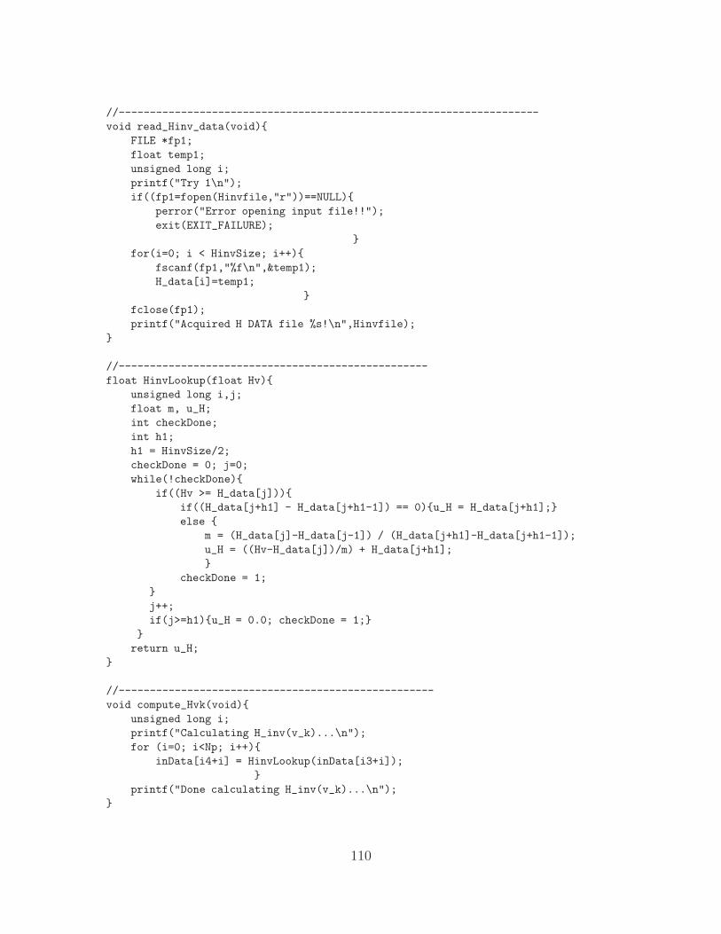
//--------------------------------------------------------------------
void read_Hinv_data(void){
FILE *fp1;
float temp1;
unsigned long i;
printf("Try 1\n");
if((fp1=fopen(Hinvfile,"r"))==NULL){
perror("Error opening input file!!");
exit(EXIT_FAILURE);
}
for(i=0; i < HinvSize; i++){
fscanf(fp1,"%f\n",&temp1);
H_data[i]=temp1;
}
fclose(fp1);
printf("Acquired H DATA file %s!\n",Hinvfile);
}
//--------------------------------------------------
float HinvLookup(float Hv){
unsigned long i,j;
float m, u_H;
int checkDone;
int h1;
h1 = HinvSize/2;
checkDone = 0; j=0;
while(!checkDone){
if((Hv >= H_data[j])){
if((H_data[j+h1] - H_data[j+h1-1]) == 0){u_H = H_data[j+h1];}
else {
m = (H_data[j]-H_data[j-1]) / (H_data[j+h1]-H_data[j+h1-1]);
u_H = ((Hv-H_data[j])/m) + H_data[j+h1];
}
checkDone = 1;
}
j++;
if(j>=h1){u_H = 0.0; checkDone = 1;}
}
return u_H;
}
//---------------------------------------------------
void compute_Hvk(void){
unsigned long i;
printf("Calculating H_inv(v_k)...\n");
for (i=0; i<Np; i++){
inData[i4+i] = HinvLookup(inData[i3+i]);
}
printf("Done calculating H_inv(v_k)...\n");
}
110

//---------------------------------------------------
void scale_data(void){
unsigned long i;
for (i=0; i<Np; i++){
inData[i1 + i] = Scale1*inData[i1 + i];
inData[i2 + i] = Scale2*inData[i2 + i];
inData[i3 + i] = Scale3*inData[i3 + i];
}
}
void zero_outputs(void){
out(0.0,board1,DAC0);out(0.0,board1,DAC1);
}
void get_offsets(void){
float temp1, temp2;int i;
temp1 = 0; temp2 = 0;
for(i=0;i<1000;i++){
//----------- read initial offset values
start_AD(board1); temp2 = temp2 + in(board1);
start_AD(board1); temp1 = temp1 + in(board1);
}
vos1 = temp1 / i;
vos2 = temp2 / i;
printf("Offset1 = %f Offset2 = %f\n",vos1,vos2);
delay(2000);
}
void cycle(int uN){
int i,j;
float temp1, o1,o2;
FILE *fp3;
if((fp3=fopen(cyclefile,"r"))==NULL){
perror("Error opening Cycle Data File!"); exit(1);
}
else{
for(i=0;i<cycleSize;i++){
fscanf(fp3,"%f\n",&temp1);
cycle_data[i]=temp1;
}
}
fclose(fp3);
for(i=0;i<uN;i++){
for(j=0;j<cycleSize;j++){
out(cycle_data[j],board1,DAC0);
start_AD(board1); o1 = in(board1); /* read */
delay(3);
printf("Cycle x [%d, %d] in: %f Out: %f\n",fileNo,j,cycle_data[j],o1);
}
}
get_offsets();
}
111

void write_data(void){
unsigned long i;
FILE *fp2;
strcpy(&outfile[0],&dummy[0]);
itoa(fileNo,&counter[0],10);
strcat(&outfile[0],&counter[0]);
if((fp2=fopen(outfile,"w"))==NULL)
printf("Error opening %s!! No data saved!\n",outfile);
else{
for(i=0; i < inSize; i++){
fprintf(fp2,"%f\n",inData[i]);
}
printf("INPUT DATA USED: %s\n",infile);
printf("ALPHA USED: %f\n",alpha);
printf("Done writing OUTPUT DATA to %s\n",outfile);
delay(2000);
fclose(fp2);
}
}
void write_temp(void){
FILE *fp2;
unsigned long i;
if((fp2=fopen(tempfile,"w"))==NULL)
printf("Error opening TEMP file!!\n");
else{
for(i=0;i < inSize;i++){
fprintf(fp2,"%f\n",inData[i]);
}
printf("Done writing TEMP file\n");
fclose(fp2);
}
}
void load_temp(void){
FILE *fp1;
float temp1;
unsigned long i;
if((fp1=fopen(tempfile,"r"))==NULL){
perror("Error opening TEMP file!!");
exit(EXIT_FAILURE);
}
for(i=0; i < inSize; i++){
fscanf(fp1,"%f\n",&temp1);
inData[i]=temp1;
}
fclose(fp1);
printf("Acquired TEMP file!\n");
}
112

void load_temp_to_vd_uk(void){
FILE *fp1;
float temp1;
unsigned long i;
if((fp1=fopen(tempfile,"r"))==NULL){
perror("Error opening TEMP file!!");
exit(EXIT_FAILURE);
}
for(i=0; i<2*Np; i++){
fscanf(fp1,"%f\n",&temp1);
inData[i]=temp1;
}
fclose(fp1);
printf("Acquired vd and uk!\n");
}
void filtfilt(void){ // zero-phase shift low-pass digital filter
unsigned long idata, lcv2, lcv3;
idata = i3;
inData[0] = 0.0;
for (lcv2=1; lcv2<Np; lcv2++){
inData[lcv2] = B*inData[lcv2-1] + A*inData[idata+lcv2-1];
}
/**** flip data ****/
for (lcv2=0; lcv2<Np; lcv2++){
lcv3 = Np-1-lcv2;
inData[idata+lcv2] = inData[lcv3];
}
/**** filter again to remove phase shift ****/
inData[0] = inData[idata];
for (lcv2=1; lcv2<Np; lcv2++){
inData[lcv2] = B*inData[lcv2-1] + A*inData[idata+lcv2-1];
}
/**** flip data back ****/
for (lcv2=0; lcv2<Np; lcv2++){
lcv3 = Np-1-lcv2;
inData[idata+lcv2] = inData[lcv3];
}
}
113

A.2 MATLAB Code
A.2.1 ICA Analysis
A sample of the MATLAB code is presented which allows the graphical presen-
tation of the ICA data over all iterations. In Fig. A.1 the inputs are shown for each
of the fifty-five iterations of the second monotonic section of the x-axis trajectory as
generated by the inverse-hysteresis ICA (3.14) with α = 0.10.
0 0.5 1 1.5-2.0
-1.0
0
1.0
2.0
Time (sec)
Inp
ut
(V)
Figure A.1: The inputs over 55 iterations of the inverse-hysteresis ICA(α = 0.10) as applied to the second monotonic section of the x-axis anddeveloped by the custom MATLAB code.
clear all;
freq = 10000; % Frequency of execution Hz
iStart = 1; % start file #
iStop = 130; % end file #
Nn = 15000; % no. of points of actual data
Nu = []; % input matrix
Nv = []; % output matrix
Calb = 3.59; %Factor 3.59 for X ONLY, 4.04 for Y
pack;
Ap = 1;
114

for i = iStart:iStop
[vd,uk,vk,Hvk] = getHilcdata(’HX16_’,i);
%%%%%%%%%%%%%%%%%%%%%%%%%%%%%%%%%%%%%%%%%%%
Nu = [Nu uk(Ap:Nn)]; %
Nv = [Nv vk(Ap:Nn)]; %
i %to monitor progress
end
vd = vd(Ap:Nn);
vd = vd*Calb;
Nv = Nv*Calb;
% calculate error
[row,col] = size(Nu);
for i = 1:col
e(i) = 100*max(abs(vd-Nv(:,i)))/(max(vd)-min(vd)); %in percent
end
k = iStart:iStart+col-1;
t = 0:1/freq:length(vd)/freq+0-1/freq;
%plot input
figure(1); clf;
plot(t,Nu); ylabel(’Input (V)’); xlabel(’Time (sec)’);
%plot output
figure(2); clf;
plot(t,Nv_14); hold on; plot(t,vd,’r--’,’LineWidth’,3);
ylabel(’Output \mum)’); xlabel(’Time (sec)’);
% plot the max error vs. k
MaxError = max(e); MinErr = min(e)
figure(3); clf;
plot(k,e,’k*-’);
xlabel(’Iteration number, k’); ylabel(’Error_{MAX} (%)’);
axis([k(1) k(col_16) 0 MaxError+3]);
%*%*%*%*%*%*%*%*%*%*%*%*%*%*%*%*%*%*%*%*%*%*%*%*%*%*%*%*%*%*%*%
% FUNCTION getHILCdata
% Assumed data in vector file of the form
% [desired_out, current_input, current_out, inverse_hyst_data]
function [vd,u,v, Hv] = getHilcdata(filename_prefix,index)
col=1;
filename_index = int2str(index);
filename = strcat(filename_prefix,filename_index);
fid=fopen(filename,’r’); % Open file for reading
dat=fscanf(fid,’%f’);
row = length(dat);
N=row/4;
115

fclose(fid);
fid=fopen(filename,’r’) ;
dat=fscanf(fid,’%f’,[col,row]);
fclose(fid);
dat=dat’;
vd = dat(1:N); u = dat(N+1:2*N);
v = dat(2*N+1:3*N); Hv = dat(3*N+1:4*N);
return
A.2.2 Hysteresis Modeling
This MATLAB code is used to model the hysteresis of individual branches of
the hysteresis behavior of the x-axis of the experimental piezoactuator. This code
first opens the previously stored file with the open loop desired, input, and output
trajectories. The MATLAB command polyfit is used to find the coefficients of the
polynomial which best fits, in the least-squares sense, the input/output data.
%%%%%%%%%%%%%%%%%%%%%%%%%%%%%%%
%%%%%%%% Model OL data %%%%%%%%
%%%%%%%% SETH ASHLEY %%%%%%%%
clear all;
Calb = 3.59; %Factor to convert output from V to um
%Load file and separate into components
f = load(’OLX04.OUT’);
xd = f(1:29000)*Calb;
xin = f(30001:59000);
xo = f(60001:89000)*Calb;
t = 0 : 1/10000 : length(xd)/10000-(1/10000);
%2nd Mono sec. of X axis
M = [2500 14503];
% Separate monotonic section
in2 = xin(M(1):M(2));
out2 = xo(M(1):M(2));
t_2 = t(M(1):M(2));
116

xd2 = xd(M(1):M(2));
% Determine 3rd order polynomial coefficients
poly2 = polyfit(in2,out2,3)
%calculate model output from actual input
for i =1:length(in2)
p_x2(i) = poly2(1)*in2(i)^3 + poly2(2)*in2(i)^2 + poly2(3)*in2(i) + poly2(4);
% compute error between modeled and actual output
e_x2(i) = (p_x2(i)-out2(i))*100/(max(out2)-min(out2));
end
%Maximum error
max_err2 = max(e_x2)
%3rd Mono sec. of X axis
M = [14504 27000];
% Separate monotonic section
in3 = xin(M(1):M(2));
out3 = xo(M(1):M(2));
t_3 = t(M(1):M(2));
xd3 = xd(M(1):M(2));
% Determine 3rd order polynomial coefficients
poly3 = polyfit(in3,out3,3)
%calculate model output from actual input
for i =1:length(in3)
p_x3(i) = poly3(1)*in3(i)^3 + poly3(2)*in3(i)^2 + poly3(3)*in3(i) + poly3(4);
% compute percent error between modeled and actual output
e_x3(i) = (p_x3(i)-out3(i))*100/(max(out3)-min(out3));
end
%Maximum error
max_err3 = max(e_x3)
% Put data together to plot
oc = [out2 ; out3];
pc = [p_x2 p_x3];
inc = [in2 ; in3];
tc = [t_x2 t_x3];
%Plot desired trajectory vs. time
figure(1);clf;
plot(t,xd,’b-.’);
hold on;
117

%Plot desired actual and modeled outputs vs. time
plot(tc,oc,’r’,tc,pc,’k--’);
% Plot hysteresis curves of measured and modeled data
figure(2);clf;
plot(inc,oc,’r’,inc,pc,’k--’);
118

Vita
Mr. Seth C. Ashley, E.I.T., was born September 1976, in
Chicago, Illinois, and is a U.S. citizen. Mr. Ashley graduated
from Whitney M. Young Magnet High School in Chicago,
Illinois and attended Oakton Community College in Des
Plaines, Illinois. He received the Bachelor of Science degree
in Electrical Engineering with a minor in Physics, cum laude
and with University Honors, from Virginia Commonwealth University in May 2006.
In August 2006, Mr. Ashley began his pursuit of a Master’s degree in Mechanical
Engineering, and received departmental support as a teaching assistant for the un-
dergraduate classes Mechatronics and Process System Dynamics. Since June 2007,
while still pursuing an advanced degree, Mr. Ashley has worked as an Electrical
Product Engineer with ALSTOM Power where he designs, develops, troubleshoots,
installs, and commissions excitation control systems, synchronizers, and protection
systems for synchronous generators.
Publications
K. K. Leang, S. C. Ashley, and G. Tchoupo, Iterative and feedback control forhysteresis compensation in SMA. Trans. ASME J. Dyn. Syst. Meas. Control,131(1):14502 (6 pages), Jan. 2009.
S. C. Ashley, U. Aridogan, R. Riddle, and K. K. Leang, Hysteresis inverse iterativelearning control of piezoactuators in AFM. In Proc. of the 17th IFAC WorldCongress, pages 8269-8274, Seoul, Korea, 6 July 2008.
S. C. Ashley, G. Tchoupo, R. M. Mohr, and K. K. Leang, Precise positioning of ashape memory alloy actuator using iterative control. In Proc. Actuator 2006Conf., Bremen, Germany, 14 June 2006.
119

Honors and Memberships
April 2006, Passed the Fundamentals of Engineering (FE) exam to earn the Engineerin Training (E.I.T.) designation
August 2006 to May 2008, Graduate and Professional Student Honor Council mem-ber
2006, Inducted into Eta Kappa Nu, The Electrical Engineering Honor Society
2005, Inducted into Tau Beta Pi, The Engineering Honors Society
2003 to Present, Member IEEE
120


![Unsupervised Deep Basis Pursuit: Learning inverse problems ...stellayu/publication/doc/2019basisNeurIPS… · Deep learning in tandem with model-based iterative optimization [2]–[6],](https://img.dokumen.tips/doc/110x75/5eca6b792047d83ea45dbaf5/unsupervised-deep-basis-pursuit-learning-inverse-problems-stellayupublicationdoc2019basisneurips.jpg)