Application of a new spectral theory of stably stratiﬁed ...netfam.fmi.fi/SSS/pdf/SGP_paper.pdf · Application of a new spectral theory of stably stratiﬁed turbulence to atmospheric

Application of a new spectral theory of stably stratified

turbulence to atmospheric boundary layers over sea ice

Semion Sukoriansky ([email protected])Department of Mechanical Engineering/Perlstone Center for AeronauticalEngineering Studies, Ben-Gurion University of the Negev, Beer-Sheva 84105, Israel

Boris Galperin ([email protected])College of Marine Science, University of South Florida, St. Petersburg, Florida33701, USA

Veniamin Perov ([email protected])Department of Research and Development, Swedish Meteorological and HydrologicalInstitute, SE-601 76 Norrkoping, Sweden

December 17, 2004

Abstract. A new spectral closure model of stably stratified turbulence is usedto develop a K − ε model suitable for applications to atmospheric boundary layers(ABLs). This K−ε model utilizes the vertical viscosity and diffusivity obtained fromthe spectral theory. In the ε-equation, the Coriolis parameter-dependent formulationof the coefficient C1 suggested by Detering and Etling is generalized to include thedependence of the Brunt-Vaisala frequency, N . The new K − ε model is testedin simulations of ABLs over sea ice and compared with the data from BASE assimulated in LES by Kosovic and Curry and data from SHEBA.

Keywords: Turbulence, Spectral theories, Stable stratification, Atmospheric bound-ary layers

1. Introduction

Atmospheric boundary layers (ABLs) are the medium moderating be-tween the atmosphere and the underlying surface. The physical pro-cesses in ABLs determine the surface fluxes of the momentum, tem-perature and humidity that are among the primary governors of theatmospheric and oceanic circulations on synoptic and global scales.Turbulence in ABL flows is strongly affected by density stratifica-tion. The subject of this paper are ABLs with stable stratification, orSBLs. Stable stratification tends to reduce the vertical mixing leadingto the development of spatial anisotropy. With increasing strength ofstratification, the near-surface layer may become pinched-off from theoverlaying circulation, essentially shielding this circulation from thesurface fluxes. Referring to this phenomenon, (Mahrt, 1998; Mahrt,1999) considered two prototype flow regimes, very stable and weaklystable, noting that in most cases, SBL flows are between these two ex-

c© 2004 Kluwer Academic Publishers. Printed in the Netherlands.

paper2.tex; 17/12/2004; 10:49; p.1

2 Sukoriansky, Galperin, Perov

tremes. The physics of the very stable SBLs are quite subtle. Althoughsuch SBLs become very shallow, down to 10 m or less (Kitaigorodskiiand Joffre, 1988; King, 1990; Zilitinkevich and Mironov, 1996; Zilitinke-vich et al., 2002a; Zilitinkevich and Baklanov, 2002; Zilitinkevich andEsau, 2002; Zilitinkevich and Esau, 2003), they still maintain well-developed turbulence (e.g., Larsen, 1990). Further analysis reveals thatthe effect of a very strong negative buoyancy force is two-fold. On theone hand, it tends to suppress vertical mixing; on the other, it enhancesvertical velocity gradient thus increasing the velocity shear and the pro-duction of the turbulent kinetic energy. These opposing actions greatlyenhance the irregularity of the flow field and its intermittency. Thispicture is further complicated by the contribution from internal wavesand their breaking (Zilitinkevich, 2002). Similar phenomena are alsoobserved in oceanic mixed layers with strong stable stratification wherelevels of turbulent energy and vertical eddy viscosity remain finite evenfor relatively large values of the Richardson number Ri (Peters et al.,1988, Cane, 1993).

Generally, spatial anisotropy and turbulence-internal wave interac-tion, features characteristic of stably stratified flows, are among the pro-cesses that are least friendly to mathematical modeling. Both phenom-ena are governed by strong nonlinearity and are not readily amenableto treatment within analytical theories. Therefore, most models eitherignore these phenomena or include them using ad hoc approximations.Modeling of SBLs presents a challenge not only to the widely usedReynolds-averaged Navier-Stokes equations-based models (RANS) butalso to large eddy simulations (LES) because strong stratification mayhave significant impact upon the subgrid-scale (SGS) modes; realisticSGS parameterizations must account for this effect.

Turbulence parameterizations used in atmospheric SBL and oceancirculation models are usually based on closure assumptions introducedin simple, nearly isotropic flows and extrapolated into real flows withstrong anisotropy and waves. However, such extrapolation may takethe closure models beyond their realm of applicability, degrading thequality of their predictive skills. Therefore, the improvement of theRANS models is an ongoing effort. Along with the RANS, alterna-tive turbulence closure models have been developed during the recentdecades. One class of such models is based upon spectral closure meth-ods (McComb, 1991). Generally, spectral closures are more complicatedthan RANS models but to their advantage, they retain more compre-hensive physics and are believed to be more accurate and general thantheir RANS counterparts. Spectral models have been widely used inanalytical theories of turbulence as well as in Large Eddy Simulations(LES) (Galperin and Orszag, 1993). Recently, we have developed a

paper2.tex; 17/12/2004; 10:49; p.2

A spectral closure model for ABL 3

new spectral closure model based upon a mapping of the velocity fieldonto a quasi-Gaussian field whose modes are governed by the Langevinequation (Sukoriansky et al., 2003). The parameters of the mappingare calculated using a systematic process of successive averaging oversmall shells of velocity and temperature modes that yields equationsfor increasingly larger-scale modes. In this procedure, the combinedcontribution of turbulence and internal waves is accounted for andthe spatial anisotropy is explicitly resolved (Sukoriansky and Galperin,2004). When the process of successive averaging is extended to thelargest scales available in the system (i.e., the turbulence macroscale),the spectral closure yields a new RANS model. This model has beenimplemented as a new version of the K − ε model and tested in single-column simulations of SBLs over sea ice. Two test cases, the BeaufortArctic Storms Experiment (BASE) and the Surface Heat Budget in theArctic program (SHEBA), were selected. This selection was stipulated,on the one hand, by the fact that the data included cases of moderateand strong stable stratification such that the new model could be putthrough a severe testing; on the other, the data has been replicatedin LES by Kosovic and Curry (2000) which, thus, could be used asa benchmark for simulations with the new K − ε model. This paperdescribes the results of these simulations. The next section provides abrief outlook of the spectral closure theory utilized in this study whilea subsequent section elaborates on the implementation of this theoryin K − ε modeling. In Section 4, results of simulations with the newK − ε model are compared with the LES of BASE and with the datafrom SHEBA. Finally, Section 5 provides discussion and conclusions.

2. The spectral closure model

The spectral closure theory is developed for a fully three-dimensional,incompressible, turbulent flow field with an imposed homogeneous,vertical, stable temperature gradient; the flow is governed by the mo-mentum, temperature and continuity equations in Boussinesq approx-imation,

∂u∂t

+ (u∇)u + αgθe3 = ν0∇2u − 1ρ∇P + f0, (1)

∂θ

∂t+ (u∇)θ +

dΘdz

u3 = κ0∇2θ, (2)

∇u = 0, (3)

where u and θ are the fluctuating velocity and the fluctuating potentialtemperature, respectively; P is the pressure, ρ is the constant reference

paper2.tex; 17/12/2004; 10:49; p.3


density, ν0 and κ0 are the molecular viscosity and diffusivity, respec-tively, α is the thermal expansion coefficient, g is the acceleration dueto gravity directed downwards, dΘ

dz is the mean potential temperaturegradient, and f0 represents a large-scale external energy source custom-arily used in spectral theories of turbulence; it maintains turbulencein statistically steady state and may originate from large-scale shearinstabilities. According to the Kolmogorov theory of turbulence, thedetails of this forcing are immaterial in statistical description; its neteffect is communicated to the fluid via a single integral parameter, therate of the energy injection at large scales. Due to strong nonlinearinteractions, the external forcing excites all Fourier modes down to thedissipative scale kd = (ε/ν3

0)1/4 (ε is the rate of viscous dissipation). Themodes exert indiscriminant, random agitation upon each other which isaccompanied by simultaneous random damping. In statistically steadystate, the processes of forcing and damping balance each other; in otherwords, every Fourier mode u(k, ω) (k and ω being Fourier space wavenumber and frequency, respectively) receives and loses equal, in statis-tical sense, amounts of energy. Reflecting the duality between nonlinearinteractions and stochastic forcing and damping, the nonlinear term inEq. (1) can be replaced by a random, modal forcing f and dampingrepresented by turbulent viscosity. The resulting linear equation withstochastic forcing and damping is known as the Langevin equation,

ui(k, ω) = Gij(k, ω)fj(k, ω). (4)

In the characterization by Kraichnan (1987), the Langevin equation canbe viewed as a device that facilitates the replacement of the originalnonlinear Navier-Stokes equation by a linear, forced, stochastic equa-tions in which the energy budget is systematically adjusted for everyFourier mode. For the temperature, a similar Langevin-type equationcan be derived; it can be shown that the role of the random forcing inthis case is assumed by the vertical velocity fluctuation (Sukorianskyand Galperin, 2004),

θ(k, ω) = −dΘdz

Gθ(k, ω)u3(k, ω). (5)

The major closure assumption of the theory is that the forcing f isquasi-Gaussian, placing the present spectral theory in the family ofthe classical quasi-Gaussian spectral closures such as the direct in-teraction approximation (DIA) (Kraichnan, 1959); the eddy-damped,quasi-normal, Markovian approximation (EDQNM)(Orszag, 1977), or,collectively, the renormalized perturbation theories (RPT) (McComb,1991). This assumption enables one to derive expressions for the eddy

paper2.tex; 17/12/2004; 10:49; p.4


viscosity and eddy diffusivity. The fluctuating velocity field is zero-mean and incompressible imposing the same restraints upon the forcingf(k, ω) in (4); in the assumption of quasi-Gaussianity, this forcing isfully determined by its two-point, two-time correlation function. Thechoice of the analytical representation of this correlation function isguided by general considerations of spatial and temporal homogeneityand incompressibility which almost completely determine its functionalform (Sukoriansky et al., 2003). By its physical meaning, the correla-tion function of the forcing f(k, ω) accounts for the statistical meanenergy input to a given mode k via its interaction with all other modessuch that its amplitude, D, is proportional to the mean rate of energytransfer through that mode. The balance between the energy gain dueto the eddy forcing and the energy loss due to the eddy dampingenables one to relate the forcing amplitude D to the dissipation rateε and the buoyancy destruction. In the case of neutral stratification,this approach recovers some basic features of isotropic homogeneousturbulence including the Kolmogorov spectrum and the Kolmogorovconstant (Sukoriansky et al., 2003; Yakhot and Orszag, 1986).

Rigorous derivation of the velocity and temperature response, orGreen functions, Gij(k, ω) and Gθ(k, ω), from the original system (1-3) is given in Sukoriansky and Galperin (2004); here, only their finalrepresentation is shown:

Gij(k, ω) = G(k, ω) [δij + A(k, ω)Pi3(k)δj3] , (6)

A(k, ω) =−N2

(−iω + νhk2h + νzk2

z)(−iω + κhk2h + κzk2

z) + N2P33(k), (7)

G(k, ω) =(−iω + νhk2

h + νzk2z

)−1, (8)

Gθ(k, ω) =(−iω + κhk2

h + κzk2z

)−1, (9)

where kh and kz are the horizontal and vertical wave numbers; νh, κh

and νz , κz are the horizontal and vertical eddy viscosities and diffusivi-ties, respectively; N ≡

√αg(dΘ/dz) is the Brunt-Vasala frequency; δij

is the Kronecker delta-symbol, and Pij(k) = δij − kikj/k2.Note that due to the effect of stable stratification, the Green’s func-

tion Gij(k, ω) has acquired tensorial properties, while eddy viscositiesand diffusivities became different in the vertical and in the horizontal.Expression (7) contains complex poles generated by the term N2P33(k)in its denominator. The real part of these poles yields a dispersionrelation for internal waves in the presence of turbulence (Sukoriansky

paper2.tex; 17/12/2004; 10:49; p.5


and Galperin, 2004),

ω2 = ω20

1 −(

k

kO

)4/3

(κzνn

− νzνn

)cos2 θ +

(κhνn

− νhνn

)sin2 θ

4 sinθ

2

,

(10)where

ω20 = N2 sin2 θ (11)

is the classical dispersion relation for linear internal waves. Here, θ isthe angle between the vector k and the vertical axis; kO = (N3/ε)1/2

is the Ozmidov wave number, and νn is the eddy viscosity in the caseof neutral stratification. The expression in the figure brackets of Eq.(10) describes internal wave frequency shift due to turbulence. In thelimit k/kO → 0 (large scales; strong stratification), the classical disper-sion relation (11) is recovered. On the other hand, on small scales,k/kO → ∞, the increasingly disorganizing action of the turbulentoverturn eventually overwhelms internal waves rendering the flow fieldpurely turbulent. The threshold of the internal waves generation in thepresence of turbulence is given by ω = 0 which, using Eq. (10), yields

kt = kO

∣∣∣∣∣4 sin θ(

κzνn

− νzνn

)cos2 θ +

(κhνn

− νhνn

)sin2 θ

∣∣∣∣∣

3/2

. (12)

Assuming that the wave radiation begins at relatively large k, at whichturbulence is still close to isotropic, the following estimates can bemade: κz/νn − νz/νn ≈ 0.4; κh/νn − νh/νn ≈ 0.4 (Sukoriansky andGalperin, 2004) yielding

kt ' kO|10 sinθ|3/2 ' 32kO| sinθ|3/2. (13)

Thus, the internal gravity waves exist only at wave numbers k smallerthan the threshold value kt.

The parameters of eddy damping are calculated using a systematicalgorithm of successive averaging over small shells of velocity and tem-perature modes which, utilizing the Langevin equations (4) and (5),yields small increments to the vertical and horizontal viscosities anddiffusivities. The details of this calculation are described in Sukorianskyand Galperin (2004); it leads to a system of four coupled ODEs forνh, νz, κh, κz,

d

dk(νh, νz , κh, κz) = −C

ε

k5R1,2,3,4(νh, νz , κh, κz), (14)

where C ' 0.7 and R1 through R4 are transcendental expressions(Sukoriansky and Galperin, 2004). These expressions are given in the

paper2.tex; 17/12/2004; 10:49; p.6


0.01 0.1 1 10 1000

0.5

1

1.5

2

2.5

Figure 1. Normalized horizontal and vertical eddy viscosities and diffusivities asfunctions of k/kO . The vertical dashed line shows the location of kt, the thresholdof internal wave generation in presence of turbulence.

Appendix for the asymptotic cases of weak and strong stratification.The computation of the viscosities and diffusivities starts at the Kol-mogorov scale kd where the initial values of νz and κz are equal totheir respective molecular values ν0 and κ0 and is continued to anarbitrary wave number k < kd. The system (14) can only be solvednumerically. Solutions obtained for the nondimensional variables νh/νn,νz/νn, κh/νn and κz/νn are presented on Fig. 1 as functions of the ratiok/kO.

At large k/kO (relatively small scales), as expected, all the nondi-mensional parameters approach the values typical of the case of neutralstratification. At small k/kO, on the other hand, approximately at thethreshold of internal wave generation, horizontal and vertical viscosi-ties and diffusivities depart markedly. Horizontal viscosity increases bya factor of 1.3 compared to the neutral case, while vertical viscositydecreases to approximately 1/6 of the horizontal viscosity value. Thevertical viscosity νz preserves a finite asymptotic value even for verystrong stable stratification. This “residual” momentum mixing may bedue to the action of internal waves which are the integral part of thepresent spectral model. It is worth of noting that the onset of internalwave radiation is concurrent with the emergence of flow anisotropy

paper2.tex; 17/12/2004; 10:49; p.7


0.1 1 100

0.5

1

1.5

2

2.5

Fr

0.01 0.1 10

0.5

1

1.5

2

2.5

Ri

Figure 2. Normalized turbulent exchange coefficients as functions of the Froudenumber Fr (left panel) and the gradient Richardson number Ri (right panel).

induced by stable stratification and the beginning of strong deviationsin eddy viscosities and diffusivities from their values in the neutral case.

Another interesting result is that κz/κh → 0 for k/kO → 0; understrong stratification, vertical diffusivity is suppressed while its hori-zontal counterpart is enhanced almost by a factor of 3 compared tothe neutral case. Flows of this kind may reveal certain features oftwo-dimensional (2D) turbulence (Cho et al., 1999).

The new spectral model can be used for simulations of turbulentshear flows with stable stratification. The scale-dependent viscositiesand diffusivities can be utilized for derivation of the respective subgrid-scale (SGS) parameters in LES. Let us denote the wave number of LESgrid resolution by kc. In many SGS parameterizations in use today, theeffect of stable stratification is not taken into account. Figure 1 providesa criterion when such an assumption is acceptable. Namely, for kc > kt,kt is given by Eq. (13), the effect of stable stratification is small suchthat the eddy viscosity and eddy diffusivity can be taken the same asin the case of neutral stratification. However, for kc < kt, the effectof stable stratification cannot be neglected; furthermore, it profoundlyincreases with decreasing ratio kc/kt. The need to improve SGS rep-resentation for LES of strongly stratified flows was emphasized in therecent GABLS report (Holtslag, 2003). The present theory provides aself-consistent framework to address this need.

The process of small scales elimination can be extended to the largestscale of turbulence identified with the integral length scale, k−1

L . Thisapproach is analogous to the Reynolds averaging and the resultingequations represent a sort of a RANS model. In the RANS format, the

paper2.tex; 17/12/2004; 10:49; p.8


non-dimensional eddy viscosities and eddy diffusivities, νh/νn, νz/νn,κh/νn and κz/νn, become functions of kL/kO. It is well known in theK−ε modeling that kL is related to the total kinetic energy of the flow,K, as kL ∝ ε/K3/2, such that kL/kO ∝ Fr3/2, where Fr = ε/KN is theFroude number. The dependence of the eddy viscosities and eddy dif-fusivities on Fr is shown on Fig. 2; more detailed derivations are givenin Sukoriansky and Galperin (2004). Alternatively, these parameterscan be represented as functions of the gradient Richardson number,Ri = N2/S2. This can be done by introducing a closure assumptionthat prescribes an equilibrium between the sum of the rate of the energydissipation, ε, and the buoyancy destruction, B (B = κzN

2), with theshear production, P (P = νzS

2, S is the magnitude of the shear). TheRi-dependent non-dimensional eddy viscosities and eddy diffusivitiesare also shown on Fig. 2. By virtue of derivation, the major featuresof the dependence on Fr and on Ri, shown in Fig. 2, replicate thoseof the dependence on k/kO shown in Fig. 1. Turbulent viscosities anddiffusivities begin to depart from their values under neutral stratifica-tion at relatively small Ri and large Fr. The most significant changein their values takes place in the range of Fr and Ri between 0.1and 1; however, the spectral theory does not predict a single value ofthe critical Richardson number, such as 1/4 according to Miles (1961)and Howard (1961) or 1 according to Abarbanel et al. (1984), at whichturbulent mixing ceases completely. For Fr < 1 and Ri > 0.1, both ver-tical viscosity and diffusivity decrease with diffusivity decreasing faster.Eventually, stable stratification may totally suppress vertical scalarmixing while vertical momentum mixing continues even at relativelyhigh Ri, apparently, due to the contribution of internal waves. Suchbehavior is not easily reproduced in RANS models or in second-momentclosure models in use in atmospheric or oceanographic modeling wherethe concept of externally imposed “residual” mixing has been routinelyutilized to account for otherwise suppressed turbulent mixing (Kanthaand Clayson, 1994; Large et al., 1994). This result is consistent withthe atmospheric and oceanic data mentioned in the Introduction thatpointed out to turbulence survival in flows with very strong stablestratification. Recent towed chain observations in the ocean (Mack andSchoeberlein, 2004) are also supportive of the gradual attenuation ofturbulence under the action of increasing stable stratification, ratherthan a sharp cut-off: “... no single critical 10-m Ri, either 0.25 (Milesand Howard) or 1 (Abarbanel et al.), is identified.”

One of the important characteristics of stably stratified turbulentflows is the behavior of the “vertical” turbulent Prandtl number, Prt =νz/κz , as a function of Ri. Figure 3 compares the prediction of the

paper2.tex; 17/12/2004; 10:49; p.9


Figure 3. Inverse turbulent Prandtl number, Pr−1t , as a function of Ri. Data points

are the observations by Kondo et al., 1978; long-dashed line refers to the model byZilitinkevich and Calanca (2000), the solid line is the present spectral theory.

present model with the observational data from Kondo et al. (1978)and a model by Zilitinkevich and Calanca (2000).

Although the general trend of Pr−1t is reproduced well for all Ri,

the theoretical values are somewhat higher than the data. Note thatpartially, this is due to the uncertainty with the value of Prt0 in neutralstratification. In the present model, Prt0 = 0.72; however, this valuemay vary between about 0.5 and 1.2 which would affect the rest ofthe curve. The broad range of variation of Pr−1

t in the data pointsout to a need for further experimental research in order to reduce thenoise-to-signal ratio.

3. Implementation of the spectral results in K − ε modelingof SBLs

The RANS models are concerned with the equations for mean hori-zontal velocities U and V and mean potential temperature Θ (PT). Inapplications to ABLs, they employ turbulent viscosity and diffusivity,KM and KH . The central problem of the RANS modeling is the deriva-tion of the appropriate expressions for KM and KH . In a standard K−εmodel used in neutrally stratified flows, the values of KM and KH are

paper2.tex; 17/12/2004; 10:49; p.10


calculated using the well-known Kolmogorov-Prandtl formulation,

KM = CµK2

ε, KH = Pr−1

t0 CµK2

ε, (15)

where the coefficient Cµ is constant and equal to 0.09 (Rodi, 1980). Asimilar value was obtained within the present spectral theory (Sukorian-sky and Galperin, 2004). In the format of K−ε modeling, the turbulentkinetic energy K and the dissipation rate ε are obtained from additionalprognostic equations. In neutral stratification, K−ε modeling has beenwell established and widely used. When the stratification is not neutral,the K − ε equations in 1D, single-column formulation take the form

DK

Dt= KM

[(∂U

∂z

)2

+(

∂V

∂z

)2]− g

Θ0KH

∂Θ∂z

− ε +∂

∂z

(Kq

∂K

∂z

), (16)

Dε

Dt=

ε

K

{C1KM

[(∂U

∂z

)2

+(

∂V

∂z

)2]− C3

g

Θ0KH

∂Θ∂z

}

− C2ε2

K+

∂

∂z

(Kε

∂ε

∂z

). (17)

The terms on the right side of Eq. (16) represent shear production,buoyant destruction, dissipation and vertical turbulent transport ofK. The terms on the right side of Eq. (17) are shear and buoyancyforcing, destruction, and vertical turbulent transport of ε. In additionto the conventional vertical eddy viscosity and diffusivity, KM andKH , respectively, Eqs. (16,17) also involve vertical turbulent mixingcoefficients for the turbulence kinetic energy and dissipation, Kq andKε, which, following Rodi (1980), have been set to Kq = KM/σq andKε = KM/σε, where σq = 1.0 and σε = 1.3. The coefficients C1, C2 andC3 are constants in a standard K − ε model. Following Rodi (1980),their values are C1 = 1.44 and C2 = 1.92 in neutral flows. Whenstratification is not neutral, the value of C3 is customarily set at 1.

In stratified flows, the K−ε formulation is affected in two aspects: (i)the coefficient Cµ in (15) is multiplied by a non-dimensional function ofstratification (the so-called stability function), and (ii) the coefficientsC1, C2 and C3 in the ε-equation may also become flow-dependent. Indealing with (i), the vertical turbulent viscosity and diffusivity, KM andKH , can be determined from a Reynolds stress model in which closureassumptions are invoked for all components of the Reynolds stress ten-sor and the heat flux vector. A well-known Reynolds stress model widelyused in meteorological and oceanographic applications is the Mellor-Yamada (MY) model and its modifications (Mellor and Yamada, 1982;

paper2.tex; 17/12/2004; 10:49; p.11


Galperin et al., 1988; Galperin and Kantha, 1989; Galperin et al., 1989;Galperin and Mellor, 1991; Kantha and Clayson, 1994, Kantha, 2003).Although the MY model employs prognostic equation for Kl ratherthan ε (l being the turbulence macroscale), the dissipation equation canreadily be implemented in that scheme. The aspect (ii) is more difficultto tackle because the ε-equation, as well as its MY counterpart, the Klequation, are not derived from any conservation law and merely followthe pattern of the turbulent energy equation (16). The problematicissues of the ε-equation have been thoroughly discussed in the literatureand will not be repeated here. Both the Reynolds stress models andthe ε-equation have problems in stratified ABLs. For instance, the MYmodels have too low values of the critical Richardson numbers at whichthe vertical turbulent mixing is suppressed (Large et al., 1994; Chenget al., 2002) while the standard K − ε model fails to replicate even aneutrally stratified ABLs (Detering and Etling, 1985).

In this paper, a new way of improving the K−ε models is suggested.The present spectral closure model is used to obtain the expressions forKM and KH thus circumventing certain shortcomings of the Reynoldsstress modeling. It is hoped that the comprehensive physical foundationof the spectral model would ensure its better performance in situationswhere the Reynolds stress closures have difficulties.

The implementation of the new spectral model in the K − ε formatsuitable for 1D, single-column simulations of SBLs is straightforward.The vertical eddy viscosity and diffusivity coefficients predicted by thespectral model, namely νz and κz , are used in place of KM and KH .Utilizing the expression for the vertical viscosity in the neutral case,

νn = CµK2

ε, (18)

where Cµ ' 0.09, one can represent KM and KH as following:

KM = αMCµK2

ε, KH = αHCµ

K2

ε, (19)

whereαM =

νz

νn, αH =

κz

νn(20)

are the aforementioned non-dimensional stability functions (note thatPrt0 in (19) is absorbed in αH). These functions can be obtained fromFig. 2 in terms of the dependence on the Froude number, Fr = ε/KN .Note that Fr is more general than Ri because the former can be usedin shearless flows. In addition, the evaluation of Ri relies upon calcu-lation of the gradients of U , V and Θ which may introduce significantnumerical errors.

paper2.tex; 17/12/2004; 10:49; p.12


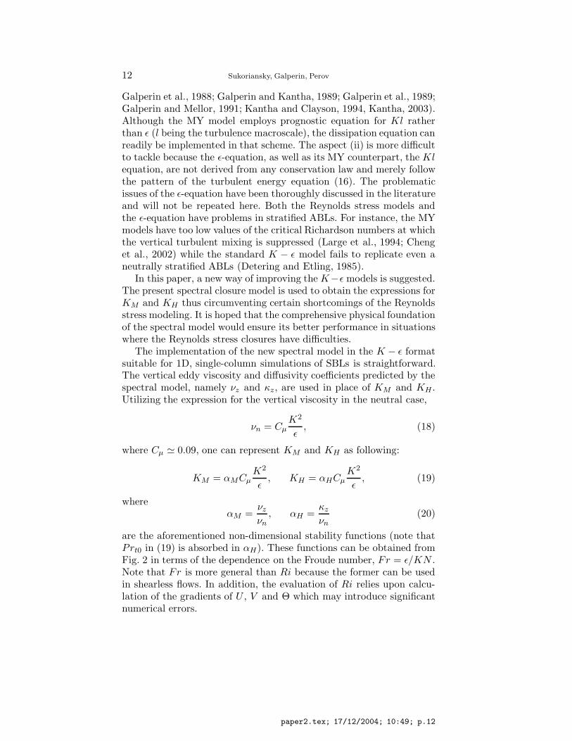
Figure 4. Comparison of stability functions calculated from the present model andfrom the MY model modified by Galperin et al. (1988).

It is of interest to compare functions αM and αH with respectivestability functions in Reynolds stress closure models. For example, inMY models, eddy viscosity and eddy diffusivity are related to stabilityfunctions, SM and SH , as

KM = qlSM , KH = qlSH, (21)

where q2 = 2K (Mellor and Yamada, 1982; Galperin et al., 1988). Com-paring (21) with (19) and using the MY relationship for the dissipation,

ε =q3

B1l, (22)

where B1 = 16.6 is one of the constants of the MY model, one obtains:

SM =(

B1

4

)CµαM , SH =

(B1

4

)CµαH . (23)

In Galperin et al. (1988), SM and SH were given as functions of GH =−(lN/q)2 which is related to the Froude number as GH = −(B1Fr/2)−2.Figure 4 compares stability functions obtained from the present spec-tral model with those from Galperin et al. (1988). A general observationis that with increasing stable stratification, both SM and SH in the MYmodel fall off quicker than their counterparts in the present spectral

paper2.tex; 17/12/2004; 10:49; p.13


model. The most significant difference is revealed in the behavior ofSM : in MY models, it becomes very small for Fr < 0.2 while in thespectral model, it remains finite even for very small values of Fr. Therapid decrease in SM may be behind the well known deficiency of theMY models to often produce insufficient mixing in flows with strongstable stratification (e.g., Kantha, 2003). The spectral model appearsto be free of this shortcoming.

Returning now to the dissipation equation, recall that when thecoefficients C1, C2 and C3 are kept constant (the standard K−ε model),the model fails to replicate a neutrally-stratified ABL (Detering andEtling, 1985). Problems arising in applications of K−ε models to ABLshave been discussed elsewhere (Rodi, 1975; Rodi, 1980; Detering andEtling, 1985). It has been realized that the constants of a standardK − ε model are not universal and various ways have been proposed tomake the constants flow-dependent. To achieve realistic description ofthe Leipzig velocity profile in neutral ABL, Detering and Etling (1985)have found it necessary to include the effect of the Earth’s rotation inthe ε-equation by making C1 dependent on the friction velocity u∗ andthe Coriolis parameter f . Their modification can be expressed in termsof the friction velocity-based Rossby number Ro∗ = u∗/|f |L,

C1 = C01 + CfRo−1

∗ , (24)

where C01 is the standard coefficient equal to 1.44, Cf = 111 is an

empirical constant and L = 0.16K3/2/ε is the turbulence macroscaleused in the K − ε modeling.

To include the effect of stable stratification, we have generalized Eq.(24) by adding a new term that depends on the friction velocity - basedFroude number Fr∗ = u∗/NL,

C1 = C01 + CfRo−1

∗ − CNFr−1∗ , (25)

where CN = 0.55 is a new empirical constant. Taking into account thatf/N ∼ 10−2 in off-equatorial regions, one can see that the rotation-and stratification-dependent terms in (25) are of the same order ofmagnitude. Note that a similar modification could be introduced in thecoefficient C3 rather than C1 in which case the correction to C0

3 = 1would have a positive sign rather than the negative sign in (25). Here,however, it was preferred to associate all the corrections with one coef-ficient, C1, and to leave the other two coefficients intact. Also note thatthe formulation (25) is just a simple lowest order (linear) approximationto the function C1(Ro−1

∗ , Fr−1∗ ). It is reasonable to assume that this

lowest order approximation would not work at large Fr−1∗ . Indeed, it

was found that a limitation

C1 ≥ C01 (26)

paper2.tex; 17/12/2004; 10:49; p.14


should be imposed on C1. Therefore, a more accurate functional formof C1 could consist of the present formulation for small and very largeFr−1

∗ , Eqs. (25) and (26), and some interpolating function for inter-mediate values of Fr−1

∗ . However, the present formulation was foundadequate for practical applications.

The K − ε model that includes prognostic equations (16) and (17)along with Eqs. (19), (20), (25) and (26) was implemented in theweather forecast model HIRLAM (High Resolution Limited Area Model)(Perov and Gollvik, 1996; Perov et al., 2001) and used to simulate SBLover sea ice. The results of these simulations are described in the nextsection.

4. Application of the new K − ε model to SBL over sea ice

Under the conditions of strong radiative cooling, the ABL over sea iceis normally clear and stably stratified. Such situation is common, forinstance, in the Arctic during the winter. Several Arctic cloud clima-tologies indicate that at winter, clear-sky conditions are observed 40 -60% of the time (Huschke, 1969; Hahn et al., 1984). During the SurfaceHeat Budget of the Arctic Ocean (SHEBA) experiment, clear-sky con-ditions were observed 27% of the winter time (Intrieri et al., 2002). TheSBL over sea ice is of a special concern for numerical weather predictionand climate modeling because of the extremely cold temperatures inthe winter Curry et al. (1996). The interest in SBLs over sea ice hasalso been stimulated by the recent attempts to interpret satellite datain situations where uncertainties in the remote sensing of sea ice lead tolarge discrepancies between surface- and satellite-derived climatologies(Rossow et al., 1993; Ramanathan et al., 1989). The properties of SBLsover ice have been studied by Tsay and Jayaweera (1984), Curry (1986),Curry et al. (1988), Fett et al. (1994), Ruffeaux et al. (1995) usingthe data collected during the Arctic Ice Dynamics Joint Experiment(AIDJEX, 1975) and the Arctic Stratus Experiment (1980). The LeadExperiment (LEADEX, 1992) was carried out to study interactionsbetween ice field with leads and SBLs (Pinto and Curry, 1995; Walteret al., 1995). The autumnal freezing period has been studied duringBASE (Paluch and Lenschow, 1997) and simulated in LES by Kosovicand Curry (2000). The Surface Heat Budget in the Arctic program(SHEBA, 1997-1998) was focused on surface fluxes at the sea ice duringdifferent seasons, particularly in the spring (Andreas et al., 1999). TheLES results for BASE and data collected during the SHEBA campaignwill be used for intercomparisons with the present K − ε model in asingle-column format.

paper2.tex; 17/12/2004; 10:49; p.15


4.1. Comparison with BASE

The main goal of BASE was to improve understanding of weathersystems in the Arctic during the fall season. BASE was conductedfrom September 19 through October 29, 1994 in the Beaufort Sea,north of the mouth of the Mackenzie River. The principal data set wasobtained from the National Center for Atmospheric Research (NCAR)C-130 aircraft. There were 14 research flights with the duration of 6 to 8hours each. These flights have provided large volumes of data coveringa wide range of SBL and sea ice conditions. The description of thedata can be found in Curry et al. (1996). In this study, the soundingsof wind and temperature, collected during flight 7 (73 N, 133 W) over afrozen sea surface, were used. No clouds were present while the potentialtemperature profile ensured strong stable stratification. The soundingsextended down to the altitude of 40 m where the temperature couldbe as low as −12.5◦C yet the well-mixed surface layer could not bereached. The surface temperature of the frozen sea was about −15◦C(corresponding to 257◦K at pressure of 1013 mb) suggesting that stablestratification could extend all the way down to the surface. The extrap-olation of the potential temperature Θ from the lowest 100 m of thesounding to the surface yields ∂Θ

∂z ∼ 0.057◦Km−1 which correspondsto the Brunt-Vaisala frequency N ∼ 0.046s−1 (Paluch and Lenschow,1997). Note that the frozen sea surface in flight 7 was not uniformas it included open leads. Since the larger leads extended over severalhundred meters and the aircraft flew only about 40 m above the surface,it was expected that the aircraft would encounter warm and moistplumes rising from the leads. However, the data from flight 7 showedno signature of such plumes. The data from flight 7 of BASE was suc-cessfully simulated in LES by Kosovic and Curry (2000) who consideredtwo cases, NLHRB and NLMR10CR. The difference between the caseswas in the rate of the surface cooling equal to 0.25◦Khr−1 in the firstcase, which was a moderately stable ABL, and 1.0◦Khr−1 in the secondcase, which was a strongly stable ABL. Thus, the BASE data coveredthe two extreme cases mentioned in the Introduction. The strengthof the overlying inversion was 0.01◦Km−1 and the surface roughnesswas 0.1m. In the LES, the transitional process of the boundary layeradjustment to the respective surface cooling rates was simulated foreach of the two cases.

Using the new K−ε model, we have simulated the same experimentsin a single-column formulation with the vertical resolution of 10 m.The boundary conditions for the turbulence characteristics at the firstgrid point are: K = 3.75u2

∗, ε = u3∗/κz, −uw = CD|U|U , −vw =

CD|U|V , −θw = CH |U|(Θ1 − Θs). Here, κ = 0.4 is the von-Karman

paper2.tex; 17/12/2004; 10:49; p.16


0

50

100

150

200

250

300

350

262 264 266 268

Hei

ght (

m)

Potential Temperature (K)

<- PTo

0

50

100

150

200

250

300

350

252 256 260 264 268

Hei

ght (

m)


<- PTo

Figure 5. Vertical profiles of mean potential temperature for the cases of moderate(left panel) and strong (right panel) stable stratification simulated with the new(solid line) and the standard (dashed-dotted line) K − ε models. The LES results byKosovic and Curry (2000) are shown by asterisks. The initial PT profiles (markedas PT0) are shown by straight solid lines.

constant, z is the distance to the surface, CD and CH are the drag andthe heat transfer coefficients, |U| is the magnitude of the near-surfacewind, Θ1 and Θs are the PT values at the first grid point and at thesurface, respectively. The CD and CH coefficients include correctiondue to the PT gradient outside of the boundary layer (Zilitinkevichand Calanca, 2000; Zilitinkevich et al., 2002b). At the upper boundary,zero values of K, ε, heat and momentum fluxes are set. Both cases ofthe moderate and strong stratification were simulated for 12 hours ofphysical time during which the flow attained a quasi-steady state. Theinitial values of the turbulent kinetic energy and dissipation were setequal to small constants. In the course of the simulations, the model“forgot” the initial distributions of K and ε after, approximately, onehour of integration.

Figure 5 shows the profiles of the potential temperature (PT) simu-lated with the new and the standard K − ε models as well as with theLES after 12 hours simulation. The agreement of the new model withthe LES data is very good for the case of moderate stratification. Thestandard model strongly overestimates the height of the temperatureboundary layer in that case. In the case of strong stratification, thesimulated temperature profile is lower than in LES. In order to un-derstand the source of this discrepancy, recall that the SGS viscositiesand diffusivities in LES by Kosovic and Curry (2000) were adopted

paper2.tex; 17/12/2004; 10:49; p.17


0

50

100

150

200

250

300

0 20 40 60

Hei

ght (

m)

Ozmidov length scale (m)

Figure 6. Left panel: mean PT profiles at different grid resolutions (the resolutionsare shown in the top left corner of the panel) for the final hour of UK MeteorologicalOffice simulations of BASE data with moderate stable stratification (courtesy ofRobert Beare, UK Met Office); right panel: vertical profiles of the Ozmidov lengthscale LO obtained from LES by Kosovic and Curry (2000) after 12 hours of simulatedtime (solid and dashed lines refer to the cases of moderate and strong stratification,respectively).

from the neutral case thus ignoring the effect of stable stratificationon SGS parameters. As discussed earlier, such an approximation isjustified when the grid size is smaller than the Ozmidov length scale,LO = π/kO. However, in strong stratification, LO decreases and maybecome comparable to or even smaller than the grid size. As evidentfrom Fig. 1, eddy viscosities and diffusivities in this case are signifi-cantly reduced compared to their values in neutral stratification. Theuse of the latters in strongly stratified flows may result in overesti-mated mixing and overpredicted boundary layer height. Since the eddydiffusivity in such flows decreases much faster than the eddy viscosity,the overprediction of the temperature boundary layer height may bemost profound. To avoid this problem, one can either increase the gridresolution or account for the effect of stratification on SGS parameters.Figure 6 substantiates these arguments. The left panel shows profiles ofpotential temperature for the moderately stratified case of BASE after 9hours of simulated time computed in LES with variable grid resolution;the model of the UK Meteorological Office has been employed in thisLES. One can see that indeed, the increase in resolution is accompaniedby the lowering of the PT profiles and sharpening of their gradients. Theright panel shows the vertical profiles of the Ozmidov scale for moderateand strong stable stratification calculated from the data in LES byKosovic and Curry (2000). In the case of the moderate stratification,the grid resolution was 5.51 m; LO remained well above this value al-most everywhere except for the top of the boundary layer such that the

paper2.tex; 17/12/2004; 10:49; p.18


0

50

100

150

200

250

300

350

-2 0 2 4 6 8 10 12

Hei

ght (

m)

Wind velocity U, V (m/s)

<- Uo

<-Vo

0

50

100

150

200

250

300

350

-2 0 2 4 6 8 10 12

Hei

ght (

m)

Wind velocity U,V (m/s)

<-Uo

<-Vo

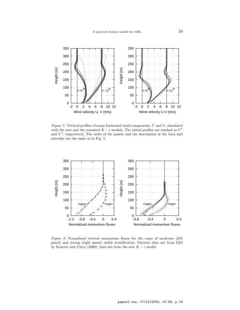
Figure 7. Vertical profiles of mean horizontal wind components, U and V , simulatedwith the new and the standard K − ε models. The initial profiles are marked as U0

and V 0, respectively. The order of the panels and the description of the lines andasterisks are the same as in Fig. 5.

0

50

100

150

200

250

300

350

-1.2 -0.8 -0.4 0 0.4

Hei

ght (

m)

Normalized momentum fluxes

<uw> <vw>

0

50

100

150

200

250

300

350

-0.8 -0.4 0 0.4

Hei

ght (

m)

Normalized momentum fluxes

<uw> <vw>

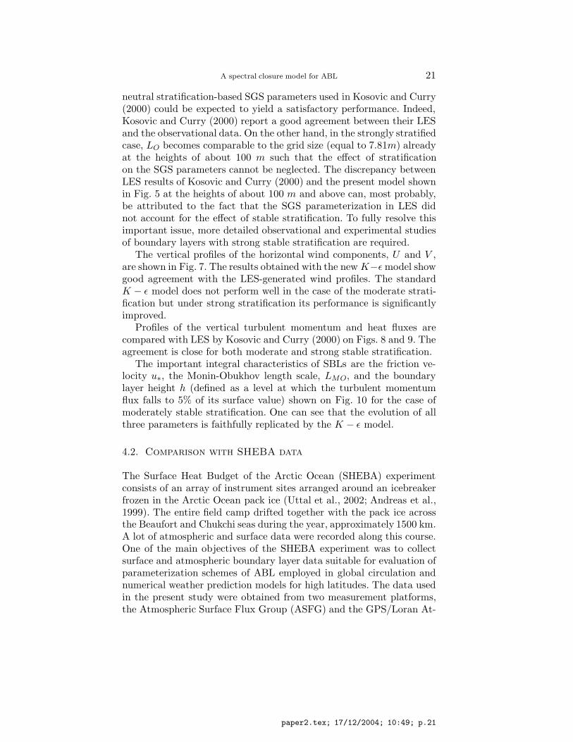
Figure 8. Normalized vertical momentum fluxes for the cases of moderate (leftpanel) and strong (right panel) stable stratification. Discrete data are from LESby Kosovic and Curry (2000), lines are from the new K − ε model.

paper2.tex; 17/12/2004; 10:49; p.19


0

50

100

150

200

250

300

350

0 0.2 0.4 0.6 0.8 1

Hei

ght (

m)

Normalized heat flux

0

50

100

150

200

250

300

350

0 0.2 0.4 0.6 0.8 1

Hei

ght (

m)

Normalized heat flux

Figure 9. Normalized vertical heat flux. The description of the panels and the datais the same as in Fig. 8

0.2

0.25

0.3

0.35

0.4

0.45

0.5

0 2 4 6 8 10 12

Fric

tion

velo

city

(m

/s)

Time (hours)

0

50

100

150

200

250

300

350

0 2 4 6 8 10 12

Hei

ght (

m)

Time (hours)

Figure 10. Friction velocity, u∗, (solid line; left panel) and Monin-Obukhov lengthscale and boundary layer height (solid and dashed lines, respectively; right panel)obtained with the new K−ε model and LES by Kosovic and Curry (2000) (asterisksand crosses). Both panels refer to the case of moderately stable stratification.

paper2.tex; 17/12/2004; 10:49; p.20


neutral stratification-based SGS parameters used in Kosovic and Curry(2000) could be expected to yield a satisfactory performance. Indeed,Kosovic and Curry (2000) report a good agreement between their LESand the observational data. On the other hand, in the strongly stratifiedcase, LO becomes comparable to the grid size (equal to 7.81m) alreadyat the heights of about 100 m such that the effect of stratificationon the SGS parameters cannot be neglected. The discrepancy betweenLES results of Kosovic and Curry (2000) and the present model shownin Fig. 5 at the heights of about 100 m and above can, most probably,be attributed to the fact that the SGS parameterization in LES didnot account for the effect of stable stratification. To fully resolve thisimportant issue, more detailed observational and experimental studiesof boundary layers with strong stable stratification are required.

The vertical profiles of the horizontal wind components, U and V ,are shown in Fig. 7. The results obtained with the new K−ε model showgood agreement with the LES-generated wind profiles. The standardK − ε model does not perform well in the case of the moderate strati-fication but under strong stratification its performance is significantlyimproved.

Profiles of the vertical turbulent momentum and heat fluxes arecompared with LES by Kosovic and Curry (2000) on Figs. 8 and 9. Theagreement is close for both moderate and strong stable stratification.

The important integral characteristics of SBLs are the friction ve-locity u∗, the Monin-Obukhov length scale, LMO, and the boundarylayer height h (defined as a level at which the turbulent momentumflux falls to 5% of its surface value) shown on Fig. 10 for the case ofmoderately stable stratification. One can see that the evolution of allthree parameters is faithfully replicated by the K − ε model.

4.2. Comparison with SHEBA data

The Surface Heat Budget of the Arctic Ocean (SHEBA) experimentconsists of an array of instrument sites arranged around an icebreakerfrozen in the Arctic Ocean pack ice (Uttal et al., 2002; Andreas et al.,1999). The entire field camp drifted together with the pack ice acrossthe Beaufort and Chukchi seas during the year, approximately 1500 km.A lot of atmospheric and surface data were recorded along this course.One of the main objectives of the SHEBA experiment was to collectsurface and atmospheric boundary layer data suitable for evaluation ofparameterization schemes of ABL employed in global circulation andnumerical weather prediction models for high latitudes. The data usedin the present study were obtained from two measurement platforms,the Atmospheric Surface Flux Group (ASFG) and the GPS/Loran At-

paper2.tex; 17/12/2004; 10:49; p.21


mospheric Sounding System. The ASFG site consisted of a 20 metersheight tower with meteorological sensors at five levels above the surface,as well as several ground based measurement platforms surroundingthe tower. The ASFG data included the surface pressure, temperature,sensible and latent heat fluxes, wind stress and albedo, and verticalprofiles of temperature and wind velocity in the lowest twenty metersof the ABL (Persson et al., 2002). The vertical profiles of temperature,humidity and winds above the ASFG tower were obtained with theVaisala radiosondes which were launched from the ship deck. In thepresent study, we used data from the winter case of 15 January, from0 to 12 hours. The values of temperature and velocity componentsabove the tower at 12 hours were obtained by linear interpolationbetween launch times. In the vertical, all radiosonde data values ateach height above the ASFG tower were smoothed using six-pointrunning mean values. At initial time, which for the winter case of 15January was characterized by strong stability, low surface temperaturewas Ts = 235◦K and the geostrophic wind velocity was Ug = 6 ms−1.During 12 hours, Ug increased to 8.2 ms−1 and Ts decreased to 233.5◦K.This process was simulated using the new K − ε model in a single-column format; the results of 12 hour integration are shown in Fig. 11.The observed vertical profile of potential temperature above ABL hadshifted during the integration period relative to the initial profile. Theanalysis of the ECMWF weather forecast for this period has showna week subsidence (negative vertical velocity) over the area of study.To reflect the ensuing processes of the large-scale vertical advectionof potential temperature and velocity, a negative vertical velocity of−10−3ms−1 was incorporated in the model. With vertical advectionaccounted for, the simulated potential temperature and velocity profilesare in good agreement with the observational data. On the other hand,Fig. 11 shows that the data cannot be reliably reproduced if the verticaladvection is not accounted for.

5. Discussion and conclusions

The spectral theory of turbulence employed in this study is based upona process of successive elimination of small scale modes that leads to amodel describing the largest scales of a flow. Partial scale eliminationcan be used to derive turbulent viscosities and diffusivities suitable forSGS parameterization in LES. The elimination of all scales leads toRANS-type models. The spectral model is derived from first principlesand is free of empirical coefficients. The model yields a dispersion rela-tion for internal waves in presence of turbulence and offers a powerful

paper2.tex; 17/12/2004; 10:49; p.22


0

50

100

150

200

250

300

232 236 240 244 248

Hei

ght (

m)


<- PTo

0

50

100

150

200

250

300

2 4 6 8 10

Hei

ght (

m)

Wind speed (m/s)

Figure 11. Vertical profiles of potential temperature (left panel) and wind speed(right panel) in SHEBA experiment. The observational data is represented by aster-isks, the simulations are shown by the thin solid lines. The short dashed lines referto the case in which the vertical advection is not accounted for.

tool to study wave-turbulence interaction. The model recognizes thehorizontal-vertical anisotropy introduced by stable stratification andprovides expressions for the horizontal and vertical turbulent viscositiesand diffusivities. The theory does not support an idea of a sharp cut-off critical Richardson number at which turbulence is fully inhibited.Instead, it predicts a transitional range of Ri in which vertical mixingis suppressed while the horizontal mixing is enhanced. The verticalturbulent viscosities and diffusivities obtained in the RANS mode (av-eraging over all scales) can be used in a K − ε model. The modificationof the coefficient C1 in the ε-equation to include the effect of stablestratification results in a general K − ε model suitable for applicationsin engineering flows as well as in neutral and stably stratified ABLs.This is a significant improvement in the K−ε modeling. The new K−εmodel has been tested in simulations of SBLs over sea ice under theconditions of moderate and strong stable stratification. The predictedpotential temperature and wind velocity, as well as the friction veloc-ity, the Monin-Obukhov length scale and the boundary layer heightare in good agreement with the corresponding values obtained in LESof BASE (Kosovic and Curry, 2000) in the case of moderately stablestratification. In the case of strong stratification, the predicted poten-tial temperature appears to slightly deviate from the LES results inthe upper part of the SBL. The source of this discrepancy has beentraced to the use of the SGS parameterization in the LES suitable

paper2.tex; 17/12/2004; 10:49; p.23


for the neutrally stratified flows. The measure of deviation of the SGSviscosities and diffusivities from their values under neutral stratificationis the ratio, kc/kO, where kc and kO are the grid resolution and theOzmidov wave numbers, respectively. When kc/kO = O(1), the effectof stable stratification on the SGS parameterization must be accountedfor. Indeed, the part of the SBL where the LES and the present resultsdiffer coincides with the region where that ratio is O(1). Additionalexperimental and/or observational data for such situations is neces-sary to fully resolve this complicated problem. Finally, the profiles ofthe mean potential temperature and wind speed predicted by the newK − ε model are in very good agreement with the observational datafrom SHEBA (Uttal et al., 2002).

This paper presents only one of the first attempts to test and vali-date the new spectral closure-based K − ε model; further comparisonswith experimental and observational data as well as with DNS andLES results are clearly needed. However, one can already see that thenew technique appears promising for practical applications and can bebeneficial if implemented in multi-dimensional circulation models.

Acknowledgements

The authors are thankful to Robert Beare from the UK Met Office forproviding the left panel of Fig. 6 and to two anonymous reviewers forconstructive suggestions. Support of this research by the ARO grantDAAD19-01-1-0816, the Israel Science Foundation grant No. 134/03,EU project “Integrated Observing and Modelling of the Arctic SeaIce and Atmosphere (IOMASA)” - EVK3-CT-2002-00067, and SwedishMeteorological and Hydrological Institute (SMHI) EU INTAS project“Representation of lakes in numerical models for environmental appli-cation” is greatly appreciated.

Appendix

A. Asymptotic cases of weak and strong stable stratification

It is convenient to introduce a spectral Froude number,

F ≡ νhk2

N, (27)

that measures the ratio of the internal wave period to the turbulenceturnover time of the mode k. The asymptotic cases of F → ∞ and

paper2.tex; 17/12/2004; 10:49; p.24


F → 0 correspond to weak and strong stratification, respectively. Inthese two cases, the expressions for R1 - R4 simplify significantly; theyare presented below.

B. Case of weak stratification, F → ∞

A small parameter expansion in powers of F−1 yields, in the lowestorder approximation,

R1 =1

5 ν2h

+ F−2

[−1

70 κh νh− 2 κh

105 (κh + νh)3+

170 (κh + νh)2

+1

70 κh (κh + νh)

]

+νh − νz

5 ν3h

, (28)

R2 =1

5 νh2

+ F−2

[−29

105 κh νh+

8 κh

105 (κh + νh)3− 4

21 (κh + νh)2+

29105 κh (κh + νh)

]

+2 (νh − νz)

15 νh3

, (29)

R3 =2

3 νh (κh + νh)

[1 − F−2 νh

10 κh+

2 (κh − κz)5 (κh + νh)

+2 (κh + 2 νh) (νh − νz)

5 νh (κh + νh)

], (30)

R4 =2

3 νh (κh + νh)

[1 − 4F−2 νh

5 κh+

κh − κz

5 (κh + νh)+

(κh + 2 νh) (νh − νz)5 νh (κh + νh)

]. (31)

C. Case of strong stratification, F → 0

In the limit F → 0, the following expressions for R1 - R4 are obtained:

R1 =164

{2

νh νz+

1−ν2

h + νh νz

+2 (κh + νh) (4 κh + 3 νh) + (22 κh + 9 νh − 15 κz − 15 νz) (κz + νz)

(κh + νh − κz − νz)3 (κz + νz)

−κz

[−2 (κh + νh)2 + (κz + νz) [9 (κh + νh) + 8 κz + 8 νz ]

]

(κh + νh − κz − νz)3 (κz + νz)

2

+ arcsinh√−1 +

νh

νz

4 νh − 3 νz

[νh (νh − νz)]32

− arcsinh

√−1 +

κh + νh

κz + νz

√κh + νh

(κh + νh − κz − νz)5

[17 κh + 20 νh + κz + νz

κh + νh

paper2.tex; 17/12/2004; 10:49; p.25


+15 (κh − κz)

κh + νh − κz − νz

]}, (32)

R2 =116

[−20 κh + 2 κz − 21 νh

(κh + νh) (κh − κz + νh − νz)2 +

κh + 2 κz + νh

(κh + νh)2 (κh − κz + νh − νz )

+2 κz

(κh + νh)2 (κz + νz)+

15 (κh − κz)(−κh + κz − νh + νz)

3

]

+arcsinh

√−1 + κh+νh

κz+νz

16√

(κh + νh) (κh − κz + νh − νz)

[−1

κh + νh+

15 (κh − κz) (κh + νh)(κh − κz + νh − νz)

3

+3 (5 κh + κz + 7 νh)(κh − κz + νh − νz)

2 +9 κh + 8 νh

(κh + νh) (−κh + κz − νh + νz)

], (33)

R3 =

√1− νz

νharcsinh

√−1 + νh

νz−

√1 − κz+νz

κh+νharcsinh

√−1 + κh+νh

κz+νz

2 (νh κz − κh νz), (34)

R4 = O(F2). (35)

References

Abarbanel, H.D., Holm, D.D., Marsden, J.E. and Ratiu, T.: 1984, ‘Richardson num-ber criterion for the nonlinear stability of three-dimensional stratified flow’, Phys.Rev. Lett. 52, 2352-2355.

Andreas, E.L., Fairall, C.W., Guest, P.S. and Persson, P.O.G.: 1999, ‘An overview ofthe SHEBA atmospheric surface flux programm. 13th Symposium on BoundaryLayers and Turbulence, Dallas, TX, Amer. Meteorol. Soc., 550–555.

Cane, M.: 1993, ‘Near-surface mixing and the ocean’s role in climate’, in: LargeEddy Simulation of Complex Engineering and Geophysical Flows, B. Galperinand S.A. Orszag, eds. Cambridge University Press, 489–509.

Cheng, Y., Canuto, V.M. and Howard, A.M.: 2002, ‘An improved model for theturbulent PBL’, J. Atmos. Sci. 59, 1550–1565.

Cho, J.Y.N., Newell, R.E. and Barrick, J.D.: 1999, ‘Horizontal wavenumber spectraof winds, temperature, and trace gases during the Pacific Exploratory Missions:2. Gravity waves, quasi-two-dimensional turbulence, and vortical modes’, J.Geophys. Res. 104, 16297–16308.

Curry, J.A.: 1986, ‘Interaction among turbulence, radiation and microphysics inArctic stratus clouds’, J. Atmos. Sci. 43, 90–106.

Curry, J.A., Ebert, E.E. and Herman, G.F.: 1988, ‘Mean and turbulence structureof the summertime Arctic cloudy boundary layer’, Quart. J. R. Meteorol. Soc.114, 715–746.

Curry, J.A., Rossow, W.B., Randall, D. and Schramm, J.L.: 1996, ‘Overview ofArctic cloud and radiation characteristics’, J. Climate 9, 1731–1764.

Detering, H. and Etling, D.: 1985, ‘Application of the E−ε model to the atmosphericboundary layer’, Boundary-Layer Meteorol. 33, 113–133.

paper2.tex; 17/12/2004; 10:49; p.26


Fett, R.W., Burk, S.D. and Thompson, W.T.: 1994, ‘Environmental phenomena ofthe Beaufort sea observed during the Leads Experiment’, Bull. Am. Meteorol.Soc. 75, 2131–2145.

Galperin, B., Kantha, L.H., Hassid, S. and Rosati, A.: 1988, ‘A quasi-equilibriumturbulent energy model for geophysical flows’, J. Atmos. Sci. 45, 55–62.

Galperin, B. and Kantha, L.H.: 1989, ‘Turbulence model for rotating flows’, AIAAJ. 27, 750–757.

Galperin, B. and Mellor, G.L.: 1991, ’The effects of streamline curvature and span-wise rotation on near-surface, turbulent boundary-layers’, J. Appl. Math. andPhysics (ZAMP) 42, 565–583.

Galperin, B. and Orszag, S., Eds. 1993: Large Eddy Simulation of ComplexEngineering and Geophysical Flows, Cambridge University Press, 622pp.

Galperin, B., Rosati, A., Kantha, L.H. and Mellor, G.L.: 1989, ‘Modeling rotatingstratified turbulent flows with application to oceanic mixed layers’, J. Phys.Oceanogr. 19, 901–916.

Hahn, C.J., Warren, S.G., London, J., Chervin, R.M., and Jenne, R.L.: 1984, ’Atlasof simultaneous occurrences of different cloud types over land’, NCAR Tech. NoteTN-241-STR, 21 pp.

Holtslag, A.A.M.: 2003, ‘GABLS initiates intercomparison for stable boundary layercase’, GEWEX News 13, 7–8.

Howard, L. N.: 1961, ‘Note on a paper of John W. Miles’, J. Fluid Mech. 10, 509-512.Huschke, R.E.: 1969, ’Arctic cloud statistics from air-calibrated surface weather

observations’, The Rand Corporation RM-6173-PR, 79 pp.Intrieri, J.M., Shupe, M.D., Uttal, T., and McCarty, B.J.: 2002, ’Annual cycle of

Arctic cloud geometry and phase from radar and lidar at SHEBA’, J. Geophys.Res. 107, 8030.

Kantha, L.H.: 2003, ‘On an improved model for the turbulent PBL’, J. Atmos. Sci.60, 2239–2246.

Kantha, L.H. and Clayson, C.A.: 1994, ‘An improved mixed-layer model forgeophysical applications’, J. Geophys. Res. 99, 25235–25266.

Kim, J. and Mahrt, L.: 1993, ‘Simple formulation of turbulent mixing in the stablefree atmosphere and nocturnal boundary layer’, Tellus 44A, 381–394.

King, J. C.: 1990, ‘Some measurements of turbulence over an Antarctic ice shelf’,Quart. J. Roy. Meteorol. Soc. 116, 379–400.

Kitaigorodskii, S. A. and Joffre, S. M.: 1988, ’In search of simple scaling for theheights of the stratified atmospheric boundary layer’, Tellus 40A, 419–443.

Kondo, J., Kanechika, O. and Yasuda, N.: 1978, ‘Heat and momentum transfer understrong stability in the atmospheric surface layer’, J. Atmos. Sci. 35, 1012–1021.

Kosovic, B. and Curry, J.A.: 2000, ‘A large eddy simulation study of a quasi-steady,stably stratified atmospheric boundary layer’, J. Atmos. Sci. 57, 1052–1068.

Kraichnan, R.H.: 1959, ‘The structure of isotropic turbulence at very high Reynoldsnumbers’, J. Fluid Mech. 5, 497–543.

Kraichnan, R.H.: 1987, ‘An interpretation of the Yakhot-Orszag turbulence theory’,Phys. Fluids 30, 2400–2405.

Large, W.G., J.C. McWilliams, and P. Niiler, 1986: Upper ocean thermal responseto strong autumnal forcing of the northeast Pacific. J. Phys. Oceanogr., 16,1524-1550.

Large, W.G., McWilliams, J.C. and S.C. Doney,: 1994, ‘Oceanic vertical mixing:A review and a model with nonlocal boundary layer parameterization’, Rev.Geophys. 32, 363–403.

paper2.tex; 17/12/2004; 10:49; p.27


Larsen, S. E., Courtney, M. and Mahrt, L.: 1990, ’Low frequency behaviour ofhorizontal power spectra in stable surface layers’, Proc. 9th AMS Symposiumon Turbulence and Diffusion, American Meteorological Society, Boston, USA,401-404.

Mack, S.A. and H.C. Schoeberlein: 2004, ’Richardson number and ocean mixing:Towed chain observations’, J. Phys. Oceanogr. 34, 736–754.

Mahrt, L.: 1998, ‘Stratified atmospheric boundary layers and breakdown of models’,Theoret. Comput. Fluid Dyn. 11, 263–279.

Mahrt, L.: 1999, ‘Stratified atmospheric boundary layers’, Boundary-Layer Meteorol.90, 375–396.

McComb, W.D.: 1991, ‘The Physics of Fluid Turbulence’, Oxford University Press,576 pp.

Mellor, G.L. Yamada, T.: 1982, ‘Development of turbulence closure model forgeophysical fluid problems’, Rev. Geophys. Space Phys. 20, 851–875.

Miles, J. W.: 1961, ‘On the stability of heterogeneous shear flows’, J. Fluid Mech.10, 496-508.

Orszag, S.A.: 1977, ‘Statistical theory of turbulence’, in Les Houches Summer Schoolin Physics, R. Balian and J.-L. Peabe, eds. Gordon and Breach, 237-374.

Paluch, I.R. and Lenschow, D.H.: 1997, ‘Arctic boundary layer in the fall seasonover open and frozen sea’, J. Geophys. Res., 102, 25955–25971.

Perov, V., Zilitinkevich, S. and Ivarsson, K.-I.: 2001, ‘Implementation of new pa-rameterisation of the surface turbulent fluxes for stable stratification in the 3-DHIRLAM’, HIRLAM Newsletter, 37, 60–66.

Persson, P.O.G., Fairall, C.W., Andreas, E.L., Guest, P.S. and Perovich, D.K.: 2002,“Measurements near the atmospheric surface flux group tower at SHEBA: Sitedescription, data processing and accuracy estimates”, NOAA Tech. Memo. OARETL.

Perov, V. and Gollvik, S.: 1996, ‘A 1-D test of a non-local K − ε boundary layerscheme for a NWP model resolution’, HIRLAM Technical Report 25.

Peters, H., Gregg, M.C. and Toole, J.M.: 1988, ‘On the parameterization ofequatorial turbulence’, J. Geophys. Res. 93, 1199–1218.

Pinto, J.O. and Curry, J.A.: 1995, ‘Atmospheric convective plumes emanating fromleads, II, Microphysical and radiative processes’, J. Geophys. Res. 100, 4633–4642.

Ramanathan, V., Cess, R.D., Harrison, E.F., Minnis, P., Barkstrom, B.R., Ahmad,E. and Hartman, D.: 1989, ‘Cloud radiative forcing and climate: Results fromthe Earth Radiative Budget Experiment’, Science 243, 63—67.

Rodi, W., 1975: ‘A note on the empirical constant in the Kolmogorov-Prandtl eddy-viscosity expression’, J. of Fluids Eng., Trans. ASME, 386–389.

Rodi, W.: 1980, ‘Turbulence models and their application in hydraulics’, Tech. Rep.Int. Assoc. for Hydraul. Res., Delft, Netherlands.

Rossow, W.B., Walker, A.W. and Garder, L.C.: 1993, ‘Comparison of ISCCP andother cloud amounts’, J. Climate 6, 2394-2418.

Ruffeaux, D., Ola, P., Persson, G., Fairall, C. and Wolfe, D.E.: 1995, ‘Ice pack andsurface energy budgets during LEADEX 1992’, J. Geophys. Res. 100, 4593-4612.

Sukoriansky, S. and Galperin, B.: 2004, ‘A spectral closure model for turbulent flowswith stable stratification’, in: Marine Turbulence - Theories, Observations andModels, H. Baumert, J. Simpson, J. Sundermann, eds., Cambridge UniversityPress, in press.

Sukoriansky, S., Galperin, B., and Staroselsky, I.: 2003, ‘Cross-term and ε-expansionin RNG theory of turbulence’, Fluid Dyn. Res. 33, 319–331.

paper2.tex; 17/12/2004; 10:49; p.28


Tsay, S.C. and Jayaweera, K.: 1984, ‘Physical characteristics of Arctic stratusclouds’, J. Clim. Appl. Meteorol 23, 584–596.

Uttal T. et al.: 2002, ‘Surface heat budget of the Arctic Ocean’, Bull. Amer. Met.Soc. 83, 255–276.

Walter, B.A., Overland, J.E. and Turet, P.: 1995, ‘A comparison of satellite-derivedand aircraft-measured surface sensible heat fluxes over the Beaufort Sea’, J.Geophys. Res. 100, 4583–4591.

Yakhot, V. and Orszag, S.A.: 1986, ‘Renormalization group analysis of turbulence.I. Basic theory’, J. Sci. Comput. 1, 3–51.

Zilitinkevich, S.: 2002, ‘Third-order transport due to internal waves and non-localturbulence in the stably stratified surface layer’, Quart, J. Roy. Met. Soc. 128,913–925.

Zilitinkevich, S.S., Baklanov, A., Rost, J., Smedman, A.-S., Lykosov, V., andCalanca, P.: 2002a, ‘Diagnostic and prognostic equations for the depth of thestably stratified Ekman boundary layer’, Quart, J. Roy. Met. Soc. 128, 25–46.

Zilitinkevich, S.S. and Baklanov, A.: 2002, ’Calculation of the height of sta-ble boundary layers in practical applications’, Boundary-Layer Meteorol. 105,389–409.

Zilitinkevich, S.S. and Calanca, P.: 2000, ‘An extended similarity - theory for thestably stratified atmospheric surface layer’, Quart. J. R. Meteorol. Soc. 126,1913–1923.

Zilitinkevich S. S. and Esau, I. N.: 2002, ‘On integral measures of the neutral,barotropic planetary boundary layers’, Boundary-Layer Meteorol. 104, 371–379.

Zilitinkevich S. S. and Esau, I. N.: 2003, ‘The effect of baroclinicity on the depthof neutral and stable planetary boundary layers’, Quart, J. Roy. Met. Soc. 129,3339–3356.

Zilitinkevich, S. and Mironov, D. V.: 1996, ‘A multi-limit formulation for the equi-librium depth of a stably stratified boundary layer’, Boundary-Layer Meteorol.81, 325–351.

Zilitinkevich, S.S., Perov , V.L., and King, J.C.: 2002b, ’ Near-surface turbulentfluxes in stable stratification: Calculation techniques for use in general-circulationmodels’, Quart. J. R. Meteorol. Soc. 128, 1571–1587.

paper2.tex; 17/12/2004; 10:49; p.29

paper2.tex; 17/12/2004; 10:49; p.30

Documents

Application of a new spectral theory of stably stratiﬁed ...netfam.fmi.fi/SSS/pdf/SGP_paper.pdf · Application of a new spectral theory of stably stratiﬁed turbulence to atmospheric