Appendix

1. Codes

The meaning of point data is defined by the parameter code:

1 - 3000 general single points 3001 - 3100 like before, with raster symbol (file with extension SIG) 3501 - 3600 like before, with vector symbol 4001 - 5000 for DTMs, in particular:

4006 significant single points, filter resistant 4007 starting points for deletion for free cut areas

5001 - 8000 general lines 8501 - 8600 like before, with vector symbol 900 I - 9999 for DTMs, in particular:

9007 limits for interpolation 9008 border polygon for free cut areas 9009 "soft" break line, if needed will be filtered 90 I 0 "hard" break line, filter resistant

For details see the LISA BASIC manual (c:\lisa\text\lisa.doc).

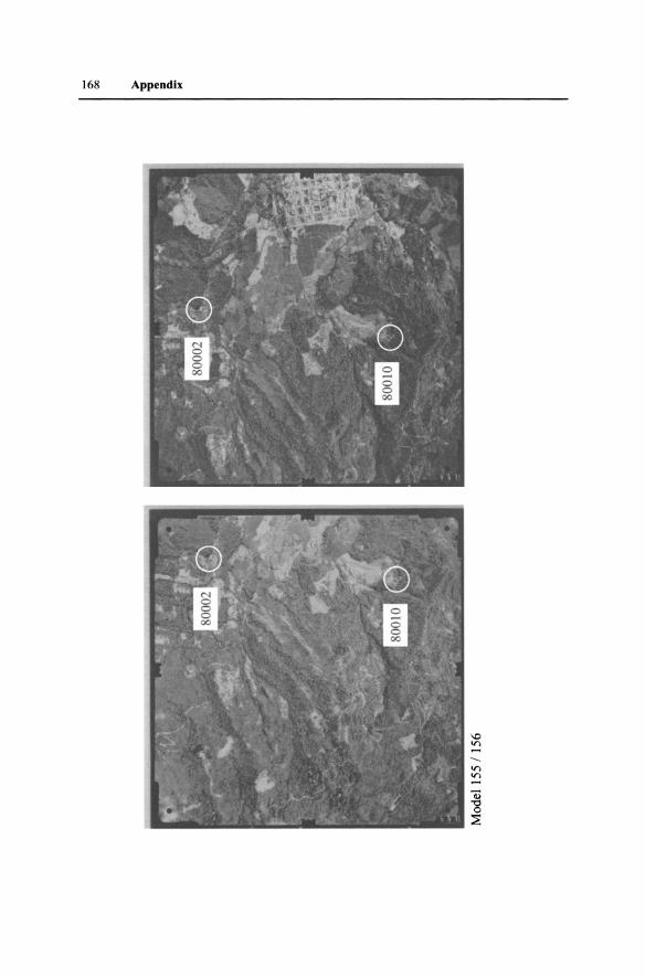
2. GCP positions for tutorial 2

On the following pages you find all of the models used in tutorial 2 (chapter 5), giving you the possibility to find the approximate positions of the GCPs.

The models are arranged in the order in which they forms the block, from left to right within each strip.

162 Appendix

Appendix 163

164 Appendix

Appendix 165

166 Appendix

Appendix 167

168 Appendix

Appendix 169

170 Appendix

Appendix 171

172 Appendix

Appendix 173

174 Appendix

Appendix 175

176 Appendix

Appendix 177

178 Appendix

1.0 1.0

Appendix 179

References

Albertz, J. & Kreiling, W. (1989): Photogrammetric Guide. 4th edition Karlsruhe, 292p. Bacher, U. (1998): Experimental Studies into Automatic DTM Generation on the DPW770. Int.

Arch. of Photogrammetry and Remote Sensing, Vol. 32, Part 4, pp 35-41. Baltsavias, P.B. & Waegli, B. (1996): Quality analysis and calibration ofDTP scanners. IAPRS,

Vol. 31, Part Bl, pp 13-19. De Lange, N. (2002) : Geoinformatik in Theorie und Praxis. Heidelberg, Berlin, New York. 438

S. Frick, W. (1995): Digitale Stereoauswertung mit der ImageStation. Zeitschrift fur Photogram­

metrie und Fernerkundung, H. I, S. 23-29. Hannah, M.J. (1988): Digital stereo image matching techniques. International Archives of Pho­

togrammetry and Remote Sensing, Vol. 27, Part B3, p 280-293. Hannah, M.J. (1989): A system for digital stereo image matching. Photogrammetric Engineering

and Remote Sensing, Vol. 55, No. 12, pp 1765-1770. Heipke c., (1990): Integration von digitaler Bildzuordnung, Punktbestimmung, Oberflachenre­

konstruktion und Orthoprojektion innerhalb der digitalen Photogrammetrie, DGK-C 366, Beck'sche Verlagsbuchhandlung, Miinchen, 89 p (PhD thesis).

Heipke, C. (1995): State-of-the-art of Digital Photogrammetric Workstations for Topographic Applications. Photogrammetric Engineering and Remote Sensing, Vol. 61, pp 49-56.

Heipke C., (1995): Digitale photogrammetrische Arbeitsstationen, DGK-C 450, Beck'sche Ver­lagsbuchhandlung, Miinchen, III p.

Heipke, C. (1996): Overview ofImage Matching Techniques. In K61bl O. (Ed.), OEEPE - Work­shop on the Application of Digital Photogrammetric Workstations, OEEPE Official Publica­tions No. 33,173-189.

Heipke, C. & Eder, K. (1998): Performance of tie-point extraction in automatic aerial triangula­tion. OEEPE Official Publication No. 35, Vol. 12, pp 125-185.

Helava, U.V. (1988): Object-space least squares correlation. Photogrammetric Engineering & Remote Sensing, Vol. 54, No.6, pp 711-714.

Hobrough, G.L. (1978): Digital online correlation. Bildmessung und Luftbildwesen, Heft 3, pp 79-86.

Jacobsen, K. (2000): Erstellung digitaler Orthophotos. GTZ Workshop zur Errichtung eines Kompetenznetzwerks fur die Sicherung von Grundstiicksrechten, Land- und Geodatenmana­gement. Hannover, 8 S.

Jacobsen, K. (2001): New Developments in Digital Elevation Modelling. GeoInformatics No.4, pp18-21.

Jacobsen, K. (2001): PC-Based Digital Photogrammetry, UN/Cospar ESA-Workshop on Data Analysis and Image Processing Techniques, Damascus, 2001, volume 13 of "Seminars of the UN Programme of Space Applications", selected Papers from Activities Held in 2001, lip.

Jacobsen, K. (2002): Programme manuals BLUH. Institute for Photogrammetry and GeoInfor­mations, University of Hannover.

Jordan / Eggert / Kneissl (1972): Handbuch der Vermessungskunde Bd. IlIa / 2. § 104 - 108. Kaufmann, V. & Ladstaedter, R. (2002): Spatio-temporal analysis of the dynamic behaviour of

the Hochebenkar rock glaciers (Oetztal Alps, Austria) by means of digital photogrammetric methods. Grazer Schriften der Geographie und Raumforschung, Bd. 37, S. 119-140.

182 References

Konecny, G. (1978): Digitale Prozessoren fUr Differentialentzerrung und Bildkorrelation. Bild­messung und Luftbildwesen, H. 3, S. 99-109.

Konecny, G. (1984): Photogrammetrie. 4. Auflage, Berlin, New York, 392 p. Konecny, G. (1994): New Trends in Technology, and their Application - Photogrammetry and

Remote Sensing - From Analogue to Digital. 13th United Nations Cartographic Conference, Beijing, China, May 9-18,1994 (World Cartography).

Konecny, G. (2002): Geoinformation. Taylor & Francis, London. Konecny, G. & Pape, D. (1980): Correlation techniques and devices. Vortrag zum XIV. ISP­

KongreB Hamburg. IPI Universitlit Hannover, Heft 6, pp 11-28. Also in: Photogrammetric Engineering and Remote Sensing, 1981, p.323-333

Kruck, E. (2002): Programme manual BINGO. GIP, Aalen. Linder, W. (1991): Klirnatisch und eruptionsbedingte Eismassenverluste am Nevado del Ruiz,

Kolumbien, wiihrend der letzten 50 Jahre. Eine Untersuchung auf der Basis digitaler Hohenmo­delle. Wiss. Arb. d. Fachr. Vermessungswesen d. Univ. Hannover, Nr. 173, 125 S. und Kartenteil.

Linder, W. & Meuser, H.-F. (1993): Automatic and interactive tiepointing. In: SAR Geocoding: Data and Systems. Karlsruhe. p 207-212.

Linder, W. (1994): Interpolation und Auswertung digitaler Gelandemodelle mit Methoden der digi­talen Bildverarbeitung. Wiss. Alb. d. Fachr. Vermessungswesen d. Univ. Hannover, Nr. 198, 101 S.

Linder, W. (1999): Geo-Informationssysteme - ein Studien- und Arbeitsbuch. Heidelberg, Ber­lin, New York. 170 S.

Lohmann, P. (2002): Segmentation and Filtering of Laser Scanner Digital Surface Models, Proc. of ISPRS Commission II Symposium on Integrated Systems for Spatial Data Production, Custodian and Decision Support, IAPRS, Volume XXXIV, part 2, pp. 311-315.

Masry, S.E. (1974): Digital correlation principles. Photogrammetric Engineering Vol. 3, pp 303-308.

Mayr, W. (2002): New exploitation methods and their relevance for traditional and modem imaging sensors. Vortrag zur 22. Wissenschaftlich-technischen Jahrestagung der DGPF, Neubrandenburg.

Miller, S.B., Helava, U.V. & De Venecia, K. (1992): Softcopy photogrammetric workstations. Photogrammetric Engineering & Remote Sensing, Vol. 58, pp 77-84.

Miller, S.B. & Walker, A.S. (1995): Die Entwicklung der digitalen photogrammetrischen Sys­teme von Leica und Helava. Zeitschrift fUr Photogrammetrie und Fernerkundung, H. 1, S. 4-15.

Mustaffar, M. & Mitchell, H.L. (2001): Improving area-based matching by using surface gradi­ents in the pixel co-ordinate transformation. ISPRS Joumal of Photogrammetry & Remote Sensing, Vol. 56, pp 42-52.

Petrie, G., Toutin, T., Rammali, H. & Lanchon, C. (2001): Chromo-Stereoscopy: 3D Stereo with orthoimages and DEM data. GeoInformatics, No.7, pp 8-11.

Plugers, P. (2000): Product Survey on Digital Photogrammetric Workstations. GIM Interna­tional, Vol. 7, pp 76-81.

Rieke-Zapp, D., Wegmann, H., Nearing, M. & Santel, F. (2001): Digital Photogrammetry for Measuring Soil Surface Roughness, In: Proceedings of the year 2001 annual conference of the American Society for Photogrammetry & Remote Sensing ASPRS, April 23-27 2001, St. Louis.

Santel, F. (2001): Digitale Nahbereichsphotogrammetrie zur Erstellung von Oberflachenmodel­len fUr Bodenerosionsversuche. Diplomarbeit, Universitlit Hannover, 119 S.

Santel, F., Heipke, C., Konnecke, S. & Wegmann, H. (2002): Image sequence matching for the determination of three-dimensional wave surfaces. Proceedings of the ISPRS Commision V Symposium, Corfu. Vol. XXXIV, part 5, pp 596-600.

Sasse, V. (1994): Beitrage zur digitalen Entzerrung auf Grund von Oberflachenrekonstruktion. Wiss. Arb. d. Fachr. Vermessungswesen d. Univ. Hannover, Nr. 199,227 p.

Schenk, T. (1999): Digital Photogrammetry, Volume I. Terra Science, Laurelville, 428 p.

References 183

Schenk, T. & Krupnik, A. (1996): Ein Verfahren zur hierarchischen Mehrfachbildzuordnung im Objektraum. Zeitschrift fur Photogrammetrie und Femerkundung, H. 1, S. 2-11.

Walker, A.S. & Petrie, G. (1996): Digital Photogrammetric Workstations 1992-96. ISPRS con­gress Vienna. International Archives of Photogrammetry and Remote Sensing, Vol. XXXI, part B2, pp 384 - 395.

Wiggenhagen, M. (2001): Geometrische und radiometrische Eigenschaften des Scanners Vexcel UltraScan 5000. Photogrammetrie, Femerkundung, Geoinformation H. 1, pp 33-37.

Willkomm, P. & Diirstel, C. (1995): Digitaler Stereoplotter PHODIS ST - Workstation Design und Automatisierung photogrammetrischer Arbeitsgange. Zeitschrift fur Photogrammetrie und Femerkundung, H. 1, S. 16-23.

Wrobel, B. & Ehlers, M. (1980): Digitale Korrelation von Femerkundungsbildem aus Wattge­bieten. Bildmessung und Luftbildwesen Nr. 48, S. 67-79.

Zhang, B. & Miller, S. (1997): Adaptive Automatic Terrain Extraction. Proceedings SPIE Vol. 3072, pp 27-36.

List of figures and formulas

1. Figures

Fig. 1: Geometry in an oriented stereo model. Changing the height in point P (on the surface) leads to a linear motion (left - right) of the points P' and P" within the photos along epipolar lines.

Fig. 2: Photos taken from different positions and with different lens angles. The Situation, view from above.

Fig. 3: The results: Photos showing the house in same size but in different repre­sentations due to the central perspective.

Fig. 4: Focal length, projection centre and rotation angles. Fig. 5: Relations between focal length J, height above ground hg and the photo

scaleflhg· Fig. 6: Photos, models and strips forming a block. Fig. 7: Flatbed DTP scanner and suggested positions ofthe photos. Fig. 8: All photos of a block should be scanned in the orientation in which they

form the block, regardless to the flight direction. Fig. 9: Shapes (first and second row) and positions (third row) of fiducial marks in

aerial photos. Fig. 10: Relations between grey values in the image and on screen. Fig. 11: Examples of natural ground control points. Fig. 12: Positions of the control points in the left image (157) Fig. 13: Positions of the control points in the right image (158) Fig. 14: Calculated versus correct graph of the function f(x) = ax + b using two,

three or more observations. Fig. 15: Test image, model 157 /158, showing the relative position of the images

and the positions of the control points. Fig. 16: Situation in the terrain and kinds of digital elevation models. Fig. 17: Relation between image positions and correlation coefficient. Fig. 18: Parts of the left and the right image, strongly zoomed. The grey values are

similar but not identical. Therefore, the correlation coefficient will not be equal but near to 1.

Fig. 19: Displacements caused by the relief, grey value differences from reflec­tions.

Fig. 20: DTM derived from image matching. Fig. 21: Central projection (images) and parallel projection (map, ortho image).

186 List of figures and formulas

Fig. 22: The resampling problem: Find the grey values for the pixels in the new image.

Fig. 23: Effect of the grey value adjustment. Fig. 24: Ortho image, 10-m contours overlaid. Fig. 25: Proposed positions of control points in the block. From JACOBSEN

2002. Fig. 26: Scheme of a block adjustment. Fig. 27: Principles of point transfer within a block. Fig. 28: Position and terrain co-ordinates of the control points. Fig. 29: Position and terrain co-ordinates of the control points (continued). Fig. 30: Part of the graphics interface for the measurement of strip connections. Fig. 31: Workflow and interchange files in BLUR. Simplified from JACOBSEN

2002. Fig. 32: Results from BLUH - Distribution of control and tie points. Fig. 33: Results from BLUH - Area covered by each image. Fig. 34: DTM mosaic, 25 m contours overlaid Fig. 35: Ortho image mosaic Fig. 36: Ortho image mosaic draped over the DTM mosaic. Fig. 37: Scan of an aerial photo on an A4 DTP scanner. Fig. 38: Test field for soil erosion, a camera position, control points. From

SANTEL 2001. Fig. 39: Situation before rain (left) and afterwards (middle), 10 m contours over­

laid, differential DTM (right). Fig. 40: The test area (above) and the camera positions on top of two houses (be-

low). Fig. 41: Approximate positions of the control points. Fig. 42: Positions ofthe control points in detail. Fig. 43: Points found by correlation, showing the wave structures. The cameras

are looking from bottom right. Fig. 44: Wave movement, time interval 0.25 seconds.

In the appendix: Stereo models and ground control point positions (for tutorial 2).

2. Formulas

1.5.1 1.7.1 1.7.2 3.2.1 3.3.1 4.2.3.1 4.3.1

Relation between height above ground, focal length and photo scale Length units Angle units Relation between pixel size [dpi] and geometric resolution [J..lm] Grey value calculated from an RGB image Brightness and contrast Co-ordinate transformations

Index

AATM 78-80,87,93,106-108, 128,142-145

Absolute orientation 30,85, 122 Adaptive threshold 79, 144 Aerial camera 3,4,5, 121 Aerial triangulation 11, 14, 15, 30,

66,67,127,128,138,143,146 Anaglyph method 43,64, 124, 139 Analysis 55,80,83,88, 107, 147,

149,150 Analytical plotter 4,8,21,29,123 Anchor points 51, 58 Approximation 47,79,107,137,

144 Area based matching 47, 154 Area sensor 3 ASCII 28,34,63, 72, 83, 88, 123,

125,153,160 Azimuth 98 Base 10,40 Batch mode 23,82,83,94, 126,

134,154,156 Bilinear 60 Block adjustment 14, 15,67,68,

79-81,83,86,88,93, 107, 129, 145-150

Blunder 80,82,85, 147-149 BMP 21-23, 100, 126 Break line 44, 135, 162 Brightness 29,31,49,60,77,129,

139,142,158 Calibration 22,27,80, 102, 103,

127-129,132 Cartesian 8, 104 Central perspective 1,3-5, 7,42,

56, 156 Central projection 57

Certain point 39-41, 106, 108, 134-136

Close-range 80, 100, 110, 121 Code 44,63,117,135,153,162 Collinear equations 37,40,43, 148 Connection point 66, 87, 90, 107,

127,138,142-145 Contours 15,32,61,62,95,97, 109 Contrast 29,31,49-53, 64, 110,

117,118,129,131,143,144, 155-158

Co-ordinate system 8, 26, 104 Correlation coefficient 39,48-56,

79,107,108,117,135-144,152-156

Correlation window 51-53,79,107, 108,117,144,154-156

Cubic convolution 60 Data collection 63 Data reduction 62, 80 Data snooping 82, 147, 149 Differential DTM 105, 108-110 Differential rectification 58 Digital camera 3,4, 10, 14,40, 103-

106, 110, 121, 127, 128, 135 Digital image processing 45, 122 Displacements 5-7,29,49,50,56,

58,87, 155 Digital situation model 58 Digital terrain model 26, 46 Elevation model 46, 47 End lap 11,21,71,107,139 Epipolar lines 2, 49 Epipolar plane 40, 44, 117 Equidistance 62, 97 Error correction 82,84-89, 147,

149,150

188 Index

Exterior accuracy 55,56 Exterior orientation 8,30-38, 66,

80,94,105-107,112-116,122, 127,130-139,151-157

Feature collection 42,44 Fiducial mark 19,21,26-29,40,

100-105,122,126-134,141,145 Filtering 61,62,97, 108, 117, 156,

157 Focal length 3,5,8-10,27,28, 102,

105, 112, 127-133, 141 Gaps 52-54,58,60, 153, 156, 157 Gauss-Krueger 8, 104 Generalisation 33 Geometric resolution 20, 26, 59, 60,

125,135,151,158 GPS 33,56, 121 Grey value adjustment 60, 61, 96,

158 Grid 45,53,54,98, 106, 133, 144,

153,160 Ground control point 32, 33, 55, 66-

69, 73, 81, 89, 150 Gruber points 69, 71, 72, 140 Height-base ratio 39, 135, 138 Hidden areas 58, 110, 112 Homologous points 73, 106-108,

126,144,155,156 Horizontal plane 8 Image space 49 Improvement 29,51,53,71,79,86,

93, 102, 107, 108, 117, 130, 132, 144, 156

Initial DTM 137,152,155,157 Interior accuracy 55 Interior orientation 8, 21, 26, 28-30,

35,37,67,69,102-105,112,127-132,137,138,141,144,148

Interpolation 46, 51, 53, 54, 58, 129,152,155,156,162

Intersection 3,40,43,49, 58, 60, 131,148,149,154

Lateral overlap 11, 141 Least squares 39, 129, 130 Lens angle 5, 6, 58 Line sensor 3

Longitudinaloverlap 11, 70, 138, 143

Matching 46-49, 52-55, 64, 72, 96, 100, 105, 108, 109, 116, 133, 152-156

Meander 11,29,129 Measuring mark 29,37,44,46,55,

101,122,123,128,130,138,141, 150,153

Metric 11,99, 104 Model area 39,40,43-46, 52, 55,

60,121,127,134,136,151-156 Model definition 30,39,93, 106,

107,115,116,122,137,151,153, 154,157

Mono measurement 64, 150 Morphologic data 44 Mosaic 15,26,60,66,93-98, 150,

153,156,157 Mounting plate 42 Nearest nadir 58,60, 157 Nearest neighbour 59 Nominal co-ordinates 27, 126, 129,

131, 132, 144, 145 Object space 43, 49 Oblique image 111, 116, 130 On-screen digiti sing 32, 159 Over-determination 30,32,37-39,

105,130 Overlay 53-56,61,62,96, 138,

150, 152, 153, 158, 159 Parallax correction 41, 122, 133-

136 Parallel projection 57 PCX 22,23, 99, 125 Plane affine transformation 29,30,

41,56,129,144,145 Pixel size 20,26,38, 124, 135 Point transfer 69, 70, 72, 139 Polygon 44,116,134,161 Polyline 44 Polynomials 133, 134 Pre-positioning 29,30,37,46,54,

128, 132, 14~ 152, 153 Principal point 104,111,127,157

Projection centre 4, 8-10, 36, 40, 44,58, Ill, 112, 120, 130-132

Projection ray 6,40,44,49, 56, 58, Ill, 154

Pyramid 100,125,143 Quicklook 71,130,143,144 Quality control 55, 136 Quality image 53,55,156 Radial-symmetric displacement 6,

49,56,133 Radiometric resolution 19,21 Rectification 56,58, 126, 136, 156,

157 Red-green glasses 15, 43, 138 Reference matrix 48 Region growing 155 Relative orientation 30, 79, 83, 121,

146, 147 Repetitive structures 50, Ill, 116,

154 Resampling 58-60 Resection in space 37,65,80, 126,

130, 133 Residuals 30,37,39,85-88, 129-

132,146,149 Resolution 20, 50, 109 Roaming 15,138,141,151,153 Robust estimators 147, 148 Rotation angles 9, 112, 120, 130 Scanner 4,5,8,11,13,14,19-22,

40,99,100, 122, 125-129,131, 132

Search matrix 48-50 Shaded relief 95, 96 Side if ormation bar 19, 21, 27, 29,

101,125,128 Side lap 11, 139, 141 Sigma naught 85

References 189

Signalised point 65 Sketch 34,36,37, 70, 71,130, 138,

141,152 Standard deviation 30,37,55,81,

85, 115, 132, 146, 148 Stereo correlation 50, 52, 93, 107,

116,153 Stereographic projection 56 Stereo measurement 17,42,52,54,

105,107,136,151,155 Stereoscopic viewing 1, II, 13,42,

56 Strip connection 72, 76, 77, 86, 88,

142,143,146,149 Subpixel improvement 29, 101,

128, 131 Superimposition 153, 158 Systematic image errors 79 Terrain model 14, 15,26,43-46,62,

95-97,108,118,151 Three-dimensional 151, 152 Threshold value 143, 154 Tie point 65, 76, 83, 87-92, 137,

141,143,147-150 TIFF 22,23,99,125 Trace 154,155 Unknowns 147 UTM 8,103 Vectordata 54,96,116,153,154,

158,159 Vector overlay 96 Vertical line locus 49 Volume 3, 108, 109 Wide angle 3,27,58, 101, 109 Window size 53, 143, 154 Working directory 25, 124 Zoom 70,97,138,141,150,153

ehe first to know with the new online notification service

Springer Alert You decide how WI keep you up to date on new publications:

• Select a specialist neld within a subjec t area

• Take your pick f rom various information formats

• (hoose how often you'd l ike to be informed

And reul .... customised informlltion to suit your needs

bJJi,i/t,.de!alert

and then you are one click away from a world of geoscience information!

Come and visit Springer's Geoscience Online Library

bJJi,i/t,.de!geO

Springer