F-1

APPENDIX FINFILTRATION MODELLING

Table of Contents

Page

F-1 Principles of Infiltration Modelling

F-1.1 Soil Properties........................................................................................................3F-1.2 Darcy’s Law..........................................................................................................4F-1.3 Concept of Vertical Infiltration.................................................................................5F-1.4 Hydrograph Separation............................................................................................6

F-2 Examples of Infiltration Models

F-2.1 The Horton Model..................................................................................................7F-2.2 Holton’s Infiltration Model......................................................................................8F-2.3 The Green-Ampt Infiltration Model..........................................................................9F-2.4 The Phi-Index Method .......................................................................................... 10F-2.5 The SCS Infiltration Model.................................................................................... 11F-2.6 Philip's 2T Infiltration Model................................................................................. 13F-2.7 GALAYER Infiltration Model............................................................................... 15F-2.8 Pond Infiltration Model (GAEXP).......................................................................... 17F-2.9 GACONST Infiltration Model................................................................................ 18F-2.10 INFEXF - Infiltration and Exfiltration Model........................................................... 20

F-3 Infiltrometers

F-3.1 ASTM Double-Ring Infiltrometer .......................................................................... 22F-3.2 Double-Cap Infiltrometer ...................................................................................... 23F-3.3 USU Recycling Furrow Infiltrometer...................................................................... 24

F-2

PageList of Figures

Figure F-1.1 Soil Moisture Hysterisis Curve ................................................................................3Figure F-1.2 Darcy’s Law - Field Representation..........................................................................4Figure F-1.3 Vertical Infiltration Schematic .................................................................................5Figure F-1.4a Hydrograph Recession Curve ..................................................................................6Figure F-1.4b Hydrograph Separation............................................................................................6Figure F-2.1 Horton’s Infiltration Model......................................................................................7Figure F-2.2 Holton’s Infiltration Model......................................................................................8Figure F-2.3 Concept: Ponded Infiltration Process........................................................................9Figure F-2.4 The Phi (φ) Index Approach .................................................................................. 10Figure F-2.5 Results: SCS Infiltration Simulation Model............................................................ 12Figure F-2.6 Homogeneous Conditions (Philip's 2T) Infiltration Simulation Model........................ 14Figure F-2.7 GALAYER Infiltration Simulation Model (Non-Homogeneous Conditions) .............. 16Figure F-2.8 GAEXP Infiltration Simulation Model (Ponded Conditions) ..................................... 17Figure F-2.9 GACONST Infiltration Simulation Model (Non-Ponding Conditions) ....................... 19Figure F-2.10 INFEXF Infiltration Simulation Model (Infiltration/Exfiltration) ............................... 21Figure F-3.1 ASTM Double-Ring Infiltrometer .......................................................................... 22Figure F-3.2 Double-Cap Infiltrometer ...................................................................................... 23Figure F-3.3 USU Recycling Furrow Infiltrometer...................................................................... 24

List of Tables

Table F-1.1 Soil Properties........................................................................................................3Table F-1.2 Bulk Density ..........................................................................................................3Table F-1.3 Darcy’s Law..........................................................................................................4Table F-1.4 Vertical Infiltration .................................................................................................5Table F-1.5 Estimation of Groundwater Storage..........................................................................6Table F-2.1 Infiltration Rate (i) and Infiltration Capacity (f) .........................................................7Table F-2.2 Holton’s Model......................................................................................................8Table F-2.2.1 Vegetation Parameters ............................................................................................8Table F-2.3 The Green-Ampt Model..........................................................................................9Table F-2.4 The Phi (φ) Index Approach .................................................................................. 10Table F-2.5 SCS Infiltration Model.......................................................................................... 11Table F-2.6 Philip's 2T Infiltration Model................................................................................. 13Table F-2.7 Model Parameters................................................................................................. 15Table F-2.8 Green-Ampt Equation ...........................................................................................15Table F-2.9 Green-Ampt Constant Flux Infiltration Model (GACONST)..................................... 18Table F-2.10 Infiltration/Exfiltration Model (INFEXF)................................................................ 20

F-3

F-1 Principles of Infiltration Modelling

F-1.1 Soil Properties

The following summarizes the infiltration process and relevant soil properties(Tables F-1.1, F-1.2, and Figure F-1.1):

Table F-1.2Bulk Density (kg/m3)

Sand 1550Gravel 1760Silt 1380Loam 1420Clay 1490All soils 1350

Table F-1.1Soil Properties

Soil porosity:

n = Vv/VT = (Vw + Va)/VT

where: Vv = volume of void, L3;VT = total volume, L3;Vw = volume of water, L3;andVa = volume of air, L3 .

Maximum storage capacity in soil, SW(max), L:

SW(max) = n. d,

where: d = depth of soil layer, L

Available volumetric water content, θ, ratio:

θ = Vw/VT

where: 0 ≤ θ ≤ n, in the order, n is 0 to.33

Water content in equivalent depth (d):SW = θ d; andSW = soil water content depth, L.

Porosity can be expressed with solid density, and dry bulkdensity:

n = 1 - ρb/ρs

where: ρb = ms/VT is dry bulk density;ρs = ms /Vs is solid density;

VT and Vs are total volume and volume of solids, L3; and Ms =mass of solids.

Soil water pressure:Ψ = Pw / γw

where: Ψ = soil water pressure head L; Pw = soil water pressure N L-2; and

λw = weight density of water NL-3.

Soil water pressure is negative in the unsaturated zone, Ψ< 0, and positive in the saturated zone, Ψ > 0.

Reference: Serrano, S.E. (1997)

Drying curve 0.4

0.3

0.2 Wetting curve 0.1

0 -150 -100 -50 0

Pressure head,? (cm)

Figure F-1.1Soil Moisture Hysterisis Curve

Hyd

raul

ic c

ondu

ctiv

ity ,

K(?

) (m

/day

)

F-4

F-1.2 Darcy’s Law

The following briefly summarizes Darcy’s Law (Table F-1.3 and Figure F-1.2):

Figure F-1.2Darcy’s Law - Field Representation

Table F-1.3Darcy’s Law

qx = Kx ix

where: qx = specific discharge LT -1 (the volumetric flowrate per unit cross-sectional area , Q x/AT)

Kx = hydraulic conductivity LT -1

ix = hydraulic gradient= dh/dx

Dynamic Darcy’s Law for saturated flow:

qx = -Kx dh/dx

Dynamic Darcy’s Law for unsaturated flow:

qx = -Kx (Ψ) dh/dx

where: Kx = hydraulic conductivity under saturatedconditions

Kx(Ψ) = hydraulic conductivity under unsaturatedconditions

Hydraulic conductivity:

K = k γ / µ

where: K = hydraulic conductivity LT-1;k = intrinsic permeability, a medium property L2;γ = specific weight of fluid NL-3; andµ = dynamic viscosity of fluid kg/(L-1T-1) .

Reference: Serrano, 1997; Chow et al, 1988

F-5

F-1.3 Concept of Vertical Infiltration

The calculation of vertical infiltration is an important component of the overallwater budget and is useful for estimating potential groundwater recharge rates(Tables F-1.4, Figure F-1.3 ).

qx AT

∆z

qx + [(∂qx / ∂z)∆z] AT

mass rate of water leaving soil

Figure F-1.3Vertical Infiltration Schematic

Table F-1.4Vertical Infiltration

Net mass rate + change of mass within volume = 0 (Figure F-1.3)

∂qx / ∂z + ∂θ / ∂t = 0

The specific moisture capacity, that is the unsaturated storageproperty – the Richard’s soil moisture equation:

C(Ψ) ∂Ψ/∂t - ∂/∂z (Kz(Ψ) ∂Ψ/∂z ) - ∂Kz(Ψ)/∂ z = 0

where: C(Ψ) = dθ / dΨ is the slope of the water content vs pressure head

Knowing that in time ∂θ/∂t = (dθ/dΨ)(∂Ψ/∂t), i. e. θ =f(Ψ)

Solution of Philip’s equation (Philip, 1957) requires knowledge ofboundary and initial soil moisture content in the soil profile.

Reference: Serrano, 1997

F-6

F-1.4 Hydrograph Separation

Hydrograph separation techniques can be used to estimate watershed infiltrationand recharge (Serrano, 1997) ( Table F-1.5, and Figures F-1.4a and F-1.4b ).

Use of water balance equation:

P – ET – I –R0 = ∆S

where: P = total precipitation, L;ET = total evaporation, L;I = total infiltration, L (interception In and

depression storage Id neglected) ;R0 = effective precipitation, L; and∆S = St2 –St1 is the change in storage; L.

With the assumption that ∆S is positive for a short term of astorm, the infiltration can be estimated:

I = P – R0 – c3 k(qt2 –qt1)/A

where: q1, q2 = flow rate at time t1 and t2;k = recession constant;c3 = a unit correction for k; andA = watershed area.

q

SR

t1 t2

time

Figure F-1.4bHydrograph Separation

Table F-1.5Estimation of Groundwater Storage

The groundwater storage, Sg, at any time, ti , underthe groundwater recession curve is the summationof baseflow rates from t1 to t2

Sg = c ∫ qt dt = c ∫qt e-t/k dt = - c k q t e

-t/k 8o

= c k qt

where: Sg = groundwater storage at time t, L3;qt = flow rate at time t, L3/T;k = groundwater recession constant(T) ;c = correction factor.

Reference: Serrano, 1997

q

t2

time

Figure F-1.4aHydrograph Recession Curve

k1 – overland flow recession

k2 – surface flow recession

k3 – groundwaterflow recession

Surface runoffvolume

Groundwater runoff volume

F-7

F-2 Examples of Infiltration Models

F-2.1 The Horton Model

The Horton model can be used to describe the concepts of infiltration rate andinfiltration capacity (Table F-2.1 and Figure F-2.1 ):

Table F-2.1Infiltration Rate (i) and Infiltration Capacity (f)

The Horton model defines:

f(t) = fc + (f0 – fc)e-kt

where: f(t) = infiltration capacity, LT-1;fc = infiltration capacity with prolonged wetting, LT-

1;f0 = initial infiltration capacity, LT -1; andk = a constant representing the rate of decrease.

Please note limitations; p(t) > f(t) for all time t, implying actualinfiltration rate i(t) equals infiltration capacity, f(t):

i(t) = f(t)

where: i(t) = the specific discharge at the ground surface; andf(t) = the intake capacity through the soil surface,

equivalent to the maximum infiltrationrate(i(max)).

Cumulative infiltration (I), depth L:

I(t) = ∑j i(j)∆t

Overland or surface runoff (SRO), depth L:

SRO(t) = P(t) – I(t)

Where: P(t) = total precipitation, L; and I(t) = infiltration, L.Horton’s model requires evaluation of f o, fc, and K (theseparameters are derived based on infiltration tests. The modelapplies when precipitation rate p(t) ,exceeds infiltration capacityf(t)

Reference: Linsley et al, 1984; Serrano, 1997

R

f0

i

I fc

time

Figure F-2.1Horton’s Infiltration Model

F-8

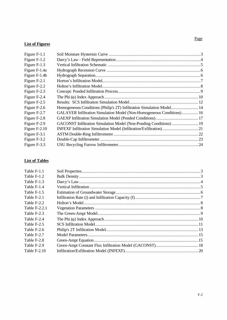
F-2.2 Holton’s Infiltration Model

The Holton model is a simple technique which specifically takes into account theeffects of vegetation ( Tables F-2.2, F-2.2.1 and Figure F-2.2 ).

Table F-2.2Holton’s Model

f = GI a Sa1.4 + fc

where: f = infiltration capacity, L;GI = growth index of vegetation;fc = infiltration capacity after prolonged wetting, L;a = surface-connected porosity; andSa = storage available in the root zone = S(max) – Sw(t), L.

The surface-connected porosity depends on the infiltration capacity of the availableStorage – a function of the density of plant roots (Table F-2.2.1). It can be estimatedFrom infiltrometer test.

Use this model when the precipitation rate is less than the infiltration capacity.

Reference: Serrano, 1997

P(t) ET(t) I(t) = min[f(t), p(t)]

Sa(t) = SMAX – SW(t)

RG(t)

Figure F-2.2Holton’s Infiltration Model

Table F-2.2.1Vegetation

Parameter, aLanduse Poor

ConditionGood

Condition

Fallow/raw crop 0.027 0.0823

Small grains/legumes

0.0548 0.0823

Hay 0.1097 0.1645

Pastures 0.2194 0.2742

Wood/forest 0.2144 0.2742

Reference: Serrano 1997.

F-9

F.2.3 The Green-Ampt Infiltration Model

The Green-Ampt model can take into account surface ponding and the movementof the wetting front ( Table F-2.3 and Figure F-2.3 ).

Table F-2.3The Green-Ampt Model

V = Ks dh/dL

where: V is flow velocity, Ks is hydraulic conductivity, and dh/dLis the hydraulic gradient.

The hydraulic gradient dh/dL, can be described in terms of thesum of the depth of pond, dp, the depth of the wetting front fromthe ground surface, Lw, and the soil suction, Scw, at the wettingfront, Lw:

dh/dL = (dp + Lw + Scw)/Lw

The total sum of infiltration I = (θs - θi)Lw

Where θsand θi are saturated and initial volume of water content.The assumption is that times t s and ti are constant as the wettingfront advances, therefore the change in I with time is:

dI/dt = d[((θs - θi)Lw]/dt = (θs -θi)dLw/dt

where: dI/dt equals Darcy’s velocity of the first equation.

Now substituting gives:

[ θs - θi) ]dLw/dt = Ks(Lw+Scw)/Lw

Rearranging: Ks/((θs - θi)dt = Lw/(Lw = Scw)dLw

Integration yields: Ktx / (θs - θi) = Scw+Lw – Scwln(Scw - Lw) + CHere, C is a constant of integration: C = Scw lnScw – Scw , at t = θ

By substituting into the yields equation gives:

Ks.t / (θs - θi) = Lw – Scw ln(1 + Lw/Scw) orKs.t = (θs - θi) Lw – Scw(θs - θi) ln(1 + Lw/Scw)

Using the cumulative infiltration and volumetric water contentgives:

Ks.t = I – Scw(θs - θi) ln[1 + I / (Scw(θs - θi) )]

Therefore, the infiltration capacity f, at any time t can be derive bytaking the derivative of the last equation:

f = Ks + Ks Scw(θs - θi) /I

Reference: McCuen, R. (1989)

Figure F-2.3Concept: Ponded Infiltration Process

F-10

F-2.4 The Phi-Index Method

This is a simple technique which is sometimes used in general water budgetmodels ( Table F-2.4 and Figure F-2.4 ).

Table F-2.4The Phi (φ) Index Approach

The phi-index represents an average rainfall intensity above which the volume of rainfallequals the volume of observed runoff. The method assumes the rate of basin rechargeremains constant during the rainfall period:

Phi-index = total basin recharge divided by the duration of rainfall

It should be noted that the phi-index overestimates infiltration rates at the start of therainfall and underestimates at the end of the event. This is due to the rate of surfaceretention and infiltration capacity which decreases with time throughout the stormperiod. Also, phi-index represents the constant rate at which water is taken from therainfall input to produce basin recharge, and it represents a combined effect ofinterception and depression storage and infiltration..

Reference: R.K. Linsley, M.A. Kohler and J.P. Paulhus (1949), Applied Hydrology, McGraw-Hill Book Co., Inc.

time

Inte

nsity

, i

Phi(φ) Basin Index

Runoff

Figure F-2.4The Phi (φ) Index Approach

F-11

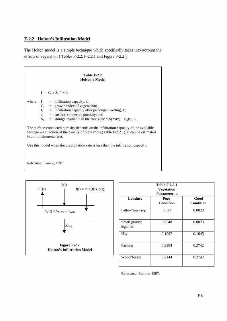
F.2.5 The SCS Infiltration Model

Simulation of water infiltration through a loamy sandy soil, e.g. a sandy material isbounded above by the soil surface and below by the groundwater table. It is important tonote that initial soil moisture content, rainfall rate and duration and surface runoffs arefactors that affect the rate of water infiltration into the soil. The purpose is to calculatethe daily infiltration amount into the soil profile. Whenever there is a lack of soilmoisture data or insufficient definition of the boundary conditions, the SCS model is asuitable semi-empirical model (USDA-SCS, 1972) ( Table F-2.5 ).

Example:

Parameter: Sw=8.2 inches, daily rainfall amount P = 0.1 to 10.0 inches is assumed.

Simulation Results: Figure F-2.5 shows the daily infiltration as a function of the dailyrainfall and surface runoff as a function of the daily rainfall. The exercise shows thatrunoff does not occur when the daily rainfall amount is smaller than 1.64 inches (0.2F=1.64 inches). Before runoff occurs, the daily infiltration equals the daily rainfall, andthe daily infiltration increases as the daily rainfall increases. However, the rate of theincrease of the daily infiltration reaches infiltration capacity at soil saturation(EPA/600/R-97/128b).

Table F-2.5SCS Infiltration Model

R = (P - 0.2Sw)2/(P + 0.8Sw)

for P > 0.2Sw

R = 0

for P 0.2Sw and

q = P - R

where:R = runoff, inches;P = daily rainfall, inches; andSw = (1000/CN) –10.

CN is based on antecedent moisture conditions

F-12

FigureF-2.5Results: SCS Infiltration Simulation Model (after EPA, 1997)

Infiltration

Sand

F-13

F-2.6 PHILIP's 2T Model

This model simulates vertical infiltration of water into a homogeneous sandy soil profile.Soil water content at the inflow-end (at the surface) is held constant and at saturation.Figure F-2.6 shows water bounded above by the soil surface and below by the ground-water table. The water depth is much greater than the water penetration depth. Hence,free water is available in excess at the surface, and the water content at the surfaceremains constant throughout the infiltration period ( Philip, 1957) ( Table F-2.6 ).

Example:

Parameters: Duration, t =1 to 24 hours is assumedInfiltration Sorptivity, S =1 cm/h½ (Philip, 1969)Constant A = 7.6 (=0.363 k ) cm/h (Jury et al, 1991)Saturated hydraulic conductivity, K= 21 cm/h (Carsel and Parrish,1988)

Simulation Results: Figure F-2.6 shows typical soil infiltration patterns, with aninfiltration rate relatively high at the onset of the infiltration. A linear relationshipbetween the cumulative infiltration and time is shown. By knowing the soil waterinfiltration rate, the movement of contaminants in the soil can now be evaluated usingother transport model equations (EPA/600/R-97/128b).

Table F-2.6Philip's 2T Infiltration Model

q(t) =1/2 S t -1/2 + A

I(t) = St1/2 + At

where: q = infiltration rate (cm/h);S = sorptivity (cm/h1/2);A = a constant (cm/h);I(t) = cumulative infiltration rate at time, t; andt = time (h).

F-14

Figure F-2.6Homogeneous Conditions (Philip's 2T) Infiltration Simulation Model

(after EPA, 1997)

Infiltration

(sand)

F-15

F-2.7 GALAYER Infiltration Model

This model describes infiltration for non-homogeneous conditions. The soil profile hasdifferent layers, and as a result the water distribution during infiltration is not uniform.Two hypothetical simulations are examined: a soil profile with two layers -- a sandylayer underlain by a loam; and a profile of three layers -- a sandy layer underlain by aloam and the loam underlain by a clay layer. Under such conditions, the sandy layercontrols the infiltration rate initially, and with time the rate of infiltration will becontrolled by the lower fine-textured layer that has the least hydraulic conductivity (Table F-2.8 )

Example:

The schematic diagrams show the layered soil profile. The thickness of the sand layer is10 cm, and the loam layer extends from the bottom of the first layer to the bottom of thesoil profile. Simulation 1 estimates water infiltration into the sand layer and continuingthrough the loam layer, while simulation 2 estimates water infiltration into three layers(sand, loam and clay). The thickness of the upper layers (sand and loam) is 10 cm. Thelowest layer (loam or clay) extends to the rest of the soil profile. The GALAYER(Flerchinger et al, 1988) model for layered soils was used. The model parameters arelisted in Table F-2.7 and infiltration results in Figure F-2.7 ).

Table F-2.7Model Parameters

Duration of Infiltration, t =1 to 24 h, is assumedSaturated Hydraulic Conductivity (Layer 1) K = 1 cm/h (Hillel, 1982)Saturated Hydraulic Conductivity (Layer 2) K = 0.5 cm/h (Hillel, 1982)Saturated Hydraulic Conductivity (Layer 3) K = 0.1 cm/h (Hillel, 1982)Change in Volumetric Water Content in (Layer 2) = 2 0.2 cm3/cm3 assumed for

Simulation 1Change in Volumetric Water Content in (Layer 3) = 2 0.1 cm3/cm3 assumed for

Simulation 2Suction Head (of Layer 2) for Simulation 1. H = 3000 cm (Hillel, 1982)Suction Head (of Layer 3) for Simulation 2. H = 7000 cm (Hillel, 1982)

Simulation Results:The infiltration rate was high at the start of the infiltration process in scenario 2. It

eventually decreased to a constant rate in time for both scenarios 1 and 2.Infiltration rate is faster in the two-layered soils as compared to the three-layered soil.

Table F-2.8Green-Ampt Equation

( see Table F-2.3 )

F-16

Figure F-2.7GAYLAYER Infiltration Simulation Model -Non-Homogeneous Conditions

(after EPA, 1997)

Infiltration (sand) 1st LAYER

Wetting Front(loam) 2nd LAYER

Sand 1 st LAYER

Loam 2nd LAYER

Clay 3rd LAYER

F-17

F-2.8 Pond Infiltration Model (GAEXP)

This model describe conditions where water infiltrates into a sandy soil under pondedconditions. Under such conditions, the infiltration rate is expected to reduce to a steady-induced rate which is equal to the saturated hydraulic conductivity. This soil profile isbounded by the soil surface water pond, and below by a groundwater table. The ExplicitGreen-Ampt model was selected. The model yields cumulative infiltration and infiltrationrate as a function of time. The model equation was to be solved iteratively (Salvucci andEntekhabi, 1994).

Example:

Parameters: Saturated Hydraulic Conductivity K= 21 cm/h (Carsel and Parrish,1988)Pond depth h =1 cm, assumedSaturated volumetric water content = 0.43 cm3 /cm3

Initial volumetric water content = 0.05 cm 3/cm3, assumed (Hillel,1982)

Simulation Results: The figure F-2.8 shows the surface infiltration and cumulativeinfiltration as a function of time. Observed is a typical soil infiltration pattern, with aninfiltration rate relatively high at the onset, then decreasing, and eventually approaching aconstant (US EPA/600/R-97/128b).

The model requires homogenous soil condition/ properties, constant and non-zeroponding depth

Figure F-2.8GAEXP Infiltration Simulation Model (Ponded Conditions)

(after EPA, 1997)

Ponding Water

Infiltration(sand)

Ponding water

Infiltration( Sand )

F-18

F-2.9 GACONST Model

This model was developed to describe infiltration into a sandy loam soil under non-ponding conditions. This soil profile is bounded above by the soil surface and below bythe groundwater table. No ponding occurs after the soil is saturated and the excess wateris discharged as surface runoff. Several infiltration models for non-ponded conditionshave been developed (Philip, 1957; Swartzendruber, 1974). In this exercise, the ConstantFlux Green-Ampt model was used (Table F-2.9 ).

Example:

Parameters: Saturated Hydraulic Conductivity K =2.59 cm/hConstant Application Rate, r = 3.5 cm/h, is assumedSaturated Volumetric Water Content = 0.41 cm3 /cm3

Initial Volumetric Water Content = 0.05 cm3 /cm3 is assumedAir exit head, he = -13.33 cmPore size index π = 0.89 (Carsel and Parrish, 1988)

Simulation Results: The figure F-2.9 shows a constant-flux infiltration pattern whenr >K. Before the surface saturation occurs at time t (5 hours), the infiltration rate isconstant and equals r, after that the infiltration rate decreases with time. The next figureillustrates a linear relationship between the cumulative infiltration and time ( EPA/600/R-97/128b).

Table F-2.9Green-Ampt Constant Flux Infiltration Model (GACONST)

When the application rate r < Ks , and t >0:

q = rI = r.t

When r > Ks , and t < t0:

q = rI = r.t

q=KS[1-(θS-θ0)hf / I

I0 = rt

Ks.( t – to) = I-Io +h f (θs - θo) Ln[(I –θs - θo )hf )/ (I o-(θs - θo)hf ] to = [K s h f (θs - θo)]/[r(r-Ks)]Where: q = surface infiltration; k s= saturated hydraulic condition; θs, θo = saturated and initial volumetric water contents, respectively; h f= capillary pressure head; t = time; r = constant water application rate; and I,Is = infiltration and initial infiltration respectively.

F-19

Figure F-2.9GACONST Infiltration Simulation Model (Non-Ponding Conditions)

(after EPA, 1997)

Infiltration( sand )

F-20

F-2.10 INFEXF - Infiltration and Exfiltration Method

The vertical movement of soil water in subsurface environments can be divided into twomajor processes: (1) infiltration and (2) exfiltration. The exfiltration process includescapillary rise, evaporation, and water uptake by plant roots (transpiration). The depth tothe groundwater table is much greater than the water penetration depth. The surfacerainfall, evaporation and transpiration are included in the model. The INFEXF modelwas chosen for the simulation (Eagleson, 1978). The initial water content before thestorm is 0.07 cm3 /cm3 This case holds for conditions when the rainfall intensity is greaterthan the infiltration capacity ( Table F-2.10 ).

Example:

The exfiltration considers a uniform initial water content of 0.20 cm3 /cm3 through andafter the storm. Also potential evaporation is assumed to be greater than the exfiltrationcapacity. The dry condition at the soil surface causes capillary rise and evaporation ofwater out of the soil surface. This exercise used the exfiltration equation.

Parameters: Saturated hydraulic conductivity K =2.59 cm/hSaturated volumetric water content = 0.41 cm3/cm3 (Carsel and Parrish,1988)Vegetated fraction M = 0.2Transpiration rate E= 0.1 cm/hInitial volumetric water content = 0.05 cm3 /cm3 assumedPore distribution index = 8.89Initial volumetric water content during interstorm period = 0.20cm3/cm3 assumed (Eagleson, 1978)

Simulation Results: The first graph of figure F-2.10 shows typical soil infiltrationpatterns, with an increase infiltration rate at the onset, then decreasing, and eventuallyapproaching a constant rate. The next graph illustrates exfiltration (actual evaporation)decreasing with time. A negative value of exfiltration indicates that exfiltration hasceased while transpiration proceeds (EPA/600R-97/128b).

Table F-2.10Infiltration/Exfiltration Model (INFEXF) Eagleson 1978.

Infiltration:

f1 = 1/2Sit-1/2 + ½ (K1 + K0 )

Exfiltration:

fe = 1/2Set-1/2 - ½ (K1 + K0 ) - MEv

where: fI and fe = infiltration and exfiltration rate (cm/h), respectively;SI and Se = infiltration and exfiltration sorptivity (cm/h1/2 ), respectively;K0 and K1 = initial and actual hydraulic conductivity (cm/h), respectively;Ev = transpiration rate (cm/h);M = vegetative fraction of land surface;t = time(h).

F-21

Figure F-2.10INFEXF Infiltration Simulation Model (Infiltration/Exfiltration)

(after EPA, 1997)

Infiltration

F-22

F.3 Infiltrometers

F-3.1 ASTM –Double Ring Infiltrometer

This device measures in-situ soil infiltration. The assembly consists of two con-centric cylinders of height = 400 mm and radius = 150 mm (inner cylinder) and300 mm (outer cylinder). A barrel (208 mm) is used as a mariotte to supply waterto each cylinder, while the flux of the inner cylinder is measured with a calibratedflow-tube-type flow meter ( Figure F-3.1 )

Figure F-3.1ASTM Double-Ring Infiltrometer

F-23

F-3.2 Double-Cap Infiltrometer

This double-cap assembly for in-situ measurement of infiltration was developedmainly to reduce the disturbance of the soil during instrument installation. Itconsists of two concentric cylinders, an inner radius of 75 mm and an outercylinder with a radius of 180 mm. Both are covered by a 10 mm thick aluminumplate. At installation, three hose fittings are attached to inlet ports, two to the outercylinder and one to the inner cylinder. Two sealed mariotte containers (25 litreseach) supply water, and the flux is measured by a flow meter that monitors in theinner compartment ( Figure F-3.2 ).

Figure F-3.2Double-Cap Infiltrometer

F-24

F-3.3 USU Recycling Furrow Infiltrometer

The recycling infiltrometer assembly consists of a small reservoir with a waterlevel recorder. Water is pumped at a fixed discharged rate to the inlets of furrowtest sections. As water flows through the test sections, it is pumped back into thereservoir. The procedure is carried out to determine the cumulative infiltration (I)as a time distribution of volumetric depletion in the reservoir. With time, a steadyinfiltration (f0) is achieved. The analysis uses the Kostiakov-Lewis equation: I =

kτa + f0 , where I = cumulative intake(vol./unit width), τ = intake opportunity time,f0 = basic intake rate (vol./unit width/unit length or time/unit time), a and k areempirical constants ( Figure F-3.3 ).

Figure F-3.3USU Recycling Furrow Infiltrometer