Embed Size (px)
Citation preview

P
ROJECT LEVE
I-69 EVAN
S
APPEEL CON
NSVILLE T
Section 5—F
ENDIX FORMIT
O INDIAN
Final Envir
OO TY DE
APOLIS TI
onmental Im
TERMINA
IER 2 STUD
mpact State
ATION
DIES
ment

Indiana Division 575 N. Pennsylvania Street, Room 254 Indianapolis, IN 46204 June 26, 2013 317-226-7475 317-226-7341 In Reply Refer To: HAD-IN Mr. Roy Nunnally, Director Asset Management, Program Engineering & Road Inventory Indiana Department of Transportation 100 N. Senate Ave. Indianapolis, Indiana 46204 Dear Mr. Nunnally: The Federal Highway Administration (FHWA) has completed the review of the enclosed Air Quality Technical Report PM 2.5 Quantitative Hot-spot analysis for I-69 Evansville to Indianapolis, Indiana: Section 5 Bloomington to Martinsville. The analysis had demonstrated transportation conformity for the project by determining that future design value concentrations for the 2018 and 2035 analysis year will be lower than the 1997 annual PM2.5 NAAQS of 15.0 μg/m³. As a result, the project does not create a violation of the 1997 annual PM2.5 NAAQS, worsen an existing violation of the NAAQS, or delay timely attainment of the NAAQS and interim milestones, which meets 40 CRF 93.116 and 93.123 and supports the project level conformity. The Indiana Department of Environmental Management (IDEM) and the United States Environmental Protection Agency (EPA) completed their reviews in accordance with the Indiana Conformity Consultation State Implementation Plan (SIP – see Enclosed USEPA and IDEM corespondence).
The Indianapolis Metropolitan Planning Organization (MPO) adopted the 2035 Long-Range Transportation Plan: 2012 Amendment that includes the approved Section 5 project corridor and corresponding “Air Quality Conformity Determination Report”, dated July 23, 2012. 1 The determination report found I-69 Section 5 to conform to the criteria outlined in the conformity rule (see Enclosed FHWA Conformity Finding dated July 23, 2012 and associated USEPA and IDEM correspondence).
1 The Indianapolis Metropolitan Planning Organization, “Indianapolis Metropolitan Planning Area, Air Quality Conformity
Determination Report, 2035 Long-Range Transportation Plan: 2012 Amendment & 2012-2015 Indianapolis Regional Transportation Improvement Program,” Indianapolis Metropolitan Planning Organization, Madison County Council of Governments, Indiana Department of Transportation, July 23, 2012, http://www.indympo.org/Plans/Documents/2035LRTP 2012Amendment Final.pdf.

2
Based on the above, we find that I-69 Section 5 conforms to all applicable project level conformity requirements. If you have any questions regarding this finding, you may contact Larry Heil at (317) 226-7480 or by e-mail [email protected].
Sincerely,
for: Richard J. Marquis Division Administrator
Enclosures Cc: Shawn Seals, IDEM
Anthony Maietta, R-5 EPA


1
Hamman, Mary Jo
From: [email protected]: Monday, June 24, 2013 3:00 PMTo: [email protected]: [email protected]: RE: I-69 Section 5 - Final PM2.5 Hot-Spot Analysis Report with Public Notices
Good Afternoon Larry! We have discussed the PM2.5 Hot‐Spot analysis process and report internally. IDEM views the PM2.5 Hot Spot analysis, as well as the associated report, as a planning requirement to demonstrate conformity with a national standard, in this case one set by the U.S. EPA. There is no direct association to an IDEM developed State Implementation Plan or rule. As such, IDEM chooses to defer official determination of this planning requirement to the Federal Highway Administration. Thanks much! Shawn
From: [email protected] [mailto:[email protected]] Sent: Tuesday, June 18, 2013 1:00 PM To: [email protected]; SEALS, SHAWN Cc: Mcmullen, Kenneth B.; Flum, Sandra; Sperry, Steve; Bales, Ronald; [email protected]; [email protected] Subject: RE: I-69 Section 5 - Final PM2.5 Hot-Spot Analysis Report with Public Notices Tony and Shawn: Attached is the final report that concludes with the following:
The analysis had demonstrated transportation conformity for the project by determining that future design value concentrations for the 2018 and 2035 analysis year will be lower than the 1997 annual PM2 5 NAAQS of 15.0 µg/m³. As a result, the project does not create a violation of the 1997 annual PM2.5
NAAQS, worsen an existing violation of the NAAQS, or delay timely attainment of the NAAQS and interim milestones, which meets 40 CRF 93.116 and 93.123 and supports the project level conformity determination.
There were no comments. So FHWA would like to issue the PM 2.5 Hot Spot conformity finding as soon as possible so we can forward the FEIS/ROD to our Headquarters for the final legal sufficiency review. Would you be able to get me your letters concurring that it is appropriate for FHWA to issue the above finding based on the attached technical report by close of business this Friday? I really appreciate all of your help in pulling this together, and I think this will provide a sound example for future such analysis. Thanks for issuing your letters as soon as you can!! Larry Heil FHWA Indiana Division
From: Bales, Ronald [mailto:[email protected]] Sent: Tuesday, June 18, 2013 12:41 PM To: Allen, Michelle (FHWA); Heil, Larry (FHWA)

2
Cc: Mcmullen, Kenneth B.; Flum, Sandra; Sperry, Steve Subject: FW: I-69 Section 5 - Final PM2.5 Hot-Spot Analysis Report with Public Notices Michelle and Larry, Please find the attached PM Hot‐Spot Technical Report provided by Michael Baker/BLA for I‐69 Section 5. Thank you. Ron Bales INDOT‐Environmental Services Division 317‐234‐4916
From: Szekeres, Dan [mailto:[email protected]] Sent: Tuesday, June 18, 2013 12:28 PM To: Bales, Ronald Cc: Hamman, Mary Jo; Miller, Tim ([email protected]) Subject: I-69 Section 5 - Final PM2.5 Hot-Spot Analysis Report with Public Notices Ron, We have updated the PM2.5 hot‐spot analysis report has follows: Within Subsection B, included reference to:
The ICG Meeting held on May 23, 2013 and that the group reviewed a preliminary version of the Technical Report, offered feedback, and advanced the document for public comment. (inserted language after Exhibit 1)
Inserted a new Subsection M (moving the Conclusion to Subsection N), entitled Public Involvement.
Noted that the Technical Report was advertised in the Martinsville Reporter‐Times and the Indianapolis Star on May 30, 2013 and June 4, 2013. A two week comment period was offered, which concluded on June 14, 2013.
Referenced the copies of the public notices in a new “Attachment F”
Noted that no comments were received during the comment period. Due to small print in the public notices, we had to preserve a high image quality which increased the WORD document size. As a result, the WORD file is available for download from our FTP site. The PDF version is attached to this email. ************ FTP LINK TO THE WORD VERSION OF TECHNICAL REPORT **********
Final (6-18-13) - I69 PM Hotspot Tech Report.docx To retrieve these attachments, click on the secure link below. https://eftp.mbakercorp.com:443?wtcQID=TVNMT05GVlNJVDpaS0tEVjVCZg==/
Access to this information will expire on 6/25/2013 12:00:00 AM ***************************************************************** As we understand, you will review, and if no comments, will forward to Larry Heil. Thanks, Dan ‐‐‐‐‐‐‐‐‐‐‐‐‐‐‐‐‐‐‐‐‐‐
Daniel Szekeres Technical Manager

3
Michael Baker Jr., Inc. 4431 North Front Street Harrisburg, PA 17110-1709 717.221.2019 (ofc) 717.579.2501 (cell) www.mbakercorp.com
Please consider the environment before printing this email.

I-69 Evansville to Indianapolis Tier 2 Studies
1
Interagency Conference Call Minutes Date: May 23, 2013 Subject: PM2.5 Hotspot Analysis: Interagency Conference Call on Technical Report Attendees:
Organization Participant Organization Participant FHWA Larry Heil Indy MPO Andrew Swenson Michele Allen Catherine Kostyn Joyce Newland IDEM Brian Callahan INDOT Ron Bales Greg Katter Baker Dan Szekeres Ying-Tzu Chung EPA Tony Maietta BLA Tim Miller
Meeting Minutes:
Larry Heil opened the conference call with an overview of the status of the I69 Section 5 PM2.5 air quality hot-spot analysis. The hot-spo t analysis technical report was provided as an attachment to the meeting appointment. The goal of the meeting was to identify i f there were any final comments on the report text and/or conclusions.
Larry provided a review of the current status and schedule:
o Finalize report by end of May 23rd. o Release public notice on May 24th for a 2-week comment period ending June 7th. o FHWA will review the summary disposi tion of comm ents and ask INDOT to
forward the final docum ent to the ICG th e week of June 10, with a request for ICG formal consultation comments within a week if possible.
o Issue the PM2.5 hot-spot conformity determination letter by the end of the week of June 17.
Tony Maietta was in acceptanc e of the docum ent as long as the comments from EPA
OTAQ were addressed (as provided in an email from Meg Patulski on 5/22/13). T he document provided for this ICG meeting addressed the comments from EPA OTAQ.

I-69 Evansville to Indianapolis Tier 2 Studies
2
IDEM (Brian Callahan) provi ded two comm ents to be ad dressed before the docum ent goes to public comment:
o Footnote the table documenting the monitor locations that monitor #2 and #3 are
“not appropriate for annual NAAQS comparison”. o Throughout the document, add “1997” before references to the PM 2.5 annual
standard. Action Items:
Baker will update the technical report to include the comments from IDEM. Baker/BLA will finalize the public notice.

1
Hamman, Mary Jo
From: [email protected]: Tuesday, April 30, 2013 9:31 AMTo: [email protected]; [email protected]; [email protected];
[email protected]; [email protected]; [email protected]; [email protected]
Cc: Szekeres, Dan; Hamman, Mary Jo; [email protected]; [email protected]; [email protected]; [email protected]; [email protected]
Subject: I-69 Section 5 PM2.5 Hot Spot Analysis ICG MinutesAttachments: Final I69 HotSpot - Meeting Minutes 041913 - Revised Per 042913 Followup....pdf; Final I69
HotSpot - Handouts ICG 041913 - Revised Per 042913 Followup Mtg.pdf; Final I69 HotSpot - Data Checklist ICG 041913 - Revised Per 042913 Followup Mtg.xlsx
Interagency Consultation Group: Attached are the Minutes from our April 19, 2013 ICG Conference Call. We had a follow‐up meeting with IDEM yesterday and determined the most recent meteorology data that is representative of our project is area is from the National Weather Service monitoring site at the Indianapolis International Airport (see http://www.in.gov/idem/airquality/2376.htm ). This data is in a format that can readily be used by AERMOD, and so we concluded it would be best to use AERMOD at this time. We expect to distribute a draft report for your review and comment the week of May 6. 2013. Timely feedback would be greatly appreciated as we would like to discuss the resolution of any comments at our ICG Meeting schedule for May 23, so it can be released for the 15‐day public comment period. OTAQ indicated they may be able to provide a suggested documentation format per their ongoing work in developing a template. Any such guidance would be much appreciated. Larry Heil FHWA Indiana Division
From: Patulski, Meg [mailto:[email protected]] Sent: Thursday, April 25, 2013 4:24 PM To: Heil, Larry (FHWA); [email protected]; Maietta, Anthony; Allen, Michelle (FHWA); [email protected]; [email protected]; Bizot, David; [email protected]; [email protected] Cc: [email protected]; Perritt, Karen (FHWA); [email protected]; [email protected]; [email protected]; [email protected]; Berry, Laura Subject: Additional information for I-69 Section 5 PM2.5 Hot Spot Analysis Tony and I have talked further about the met data issues that were discussed on last Friday’s conference call for the I‐69, Section 5 PM hot‐spot analysis. We wanted to share new information that could help inform the analysis. 1. We wanted to confirm our support for the MOVES input approach for temperature and humidity. The 4/19/13 draft checklist described these inputs as: “Monthly average meteorology data for each hour by month. Use same inputs as developed for PM2.5 SIP (Marion County inputs) to calculate average temperatures/humidity for each representative time period.” We support this approach for the PM hot‐spot analysis. 2. We also support the approach for the CAL3QHCR input data (i.e., using “Meteorology inputs from EPA’s SCRAM website”) if the met data is representative of the project area. On the Friday call, I raised concerns regarding the age of the data on the SCRAM site, but I now believe it is reasonable and consistent with EPA’s Guidance if the data is representative.

2
Section 7.5.1 of EPA’s Quantitative PM Hot‐spot Guidance states that “One of the key factors in producing credible results in a PM hot‐spot analysis is the use of meteorological data that is as representative as possible of the project area.” The selection of a representative met station is something that is decided through the consultation process, and the guidance describes several factors to consider in deciding whether met data for air quality modeling is representative, e.g., “The proximity of the project area to the meteorological monitoring site” and “The similarity of the project area to the meteorological monitoring site in surface characteristics.” The guidance states that “five consecutive years of the most recent representative meteorological data should be used,” but also states that EPA’s SCRAM site contains additional information, including “archived meteorological data (which may be suitable for some analyses).” I hope these clarifications are helpful in providing certainty in developing your project analysis. I will return to the office on Tuesday, and can answer any additional questions if needed. Meg Patulski, EPA‐OTAQ

I-69 Evansville to Indianapolis Tier 2 Studies
1
Interagency Conference Call Minutes Date: April 19, 2013 (Includes Revisions based on 4-29-13 Meeting/Call with IDEM/FHWA/INDOT/Consultants) Subject: I69 Section 5 PM 2.5 Hotspot Analysis: Interagency Conference Call on Methodology Attendees:
Organization Participant Organization Participant FHWA Larry Heil Indy MPO Andrew Swenson Michele Allen Stephanie Belch Karen Perritt IDEM Gale Ferris INDOT Ron Bales Greg Katter Baker Mary Jo Hamman Dan Szekeres EPA Meg Patulski Ying-Tzu Chung David Bizot Rob D’Abadie Tony Maietta BLA Tim Miller
Meeting Minutes: Project Overview: Larry Heil opened the conference call with an overview of the I69 Section 5 project. This section of the project does not include additiona l travel lanes and is focused on upgrading the roadway to a lim ited-access facility with inte rchanges. Section 4 is under construction and Section 6 is in the MPO confor mity analysis for construction during the 2016-2035 time period after Section 5 has opened to traffic. The PDF handout file (attached to m inutes) was reviewed to identify key m ethodology and approach issues requiring interagency concurre nce (as indicated on page 1 of the handout). These topics are addressed in the following sections. Need for PM2.5 Hotspot Analysis (Handout Page 2): Larry Heil indicated that FHWA does not con sider this p roject as a Project of Air Quality Concern. Forecasts ind icate small increases in trucks (+351 per day) in 2018. Larger truck increases are forecasted in 2035 but emission factors are expected to be much lower than current values.

I-69 Evansville to Indianapolis Tier 2 Studies
2
Meg Patulski indicated that OTAQ believes th is project is a Project o f Air Quality Concern. Tony Maietta of EPA’s regional office deferred to OTAQ in providing the recommendation. The ICG group concurred that a project level hots pot analysis would be conducted f or Section 5 despite not having a unanimous decision on it being a Project of Air Quality Concern. Analysis Approach (Handout Page 3-4): Larry Heil provided an overview of the analys is approach. The approach will utilize EPA’s guidance (EPA-420-B-10-040) and will in itially focus on the Build con dition of th e preferred alternative. Design values will be calcu lated for each an alysis year and com pared to the NAAQS. The ICG concurred with the project approach. Analysis Study Area (Handout Page 5): Larry Heil provided a description of the analysis study area that includes the interchange with SR 39. This study area falls within Section 6 not Section 5. Meg Patulski of OTAQ agreed with the selection of the project location and indicated that the intent of the guida nce was followed. The ICG concurred with the analysis study area. Analysis Years (Handout Page 6): Larry Heil indicated the analysis years based on the available m odeling. The years include the opening year (2018) and a horizon year (2035). Despite having m uch lower trucks, the opening year is estimated to have higher em issions based on an initial analysis of emission factors from EPA’s MOVES model conducted by Baker. Due to the difficulties in selecting only one of these years, FHWA has recommended that both analysis years be included in the analy sis. The I CG concurred with this decision. Type of PM for Analysis (Handout Page 7): Dan Szekeres of Baker provided an overview of what pollutants will be included in the hotspot analysis. Analyses will include directly emitted PM2.5 with a focus on only the freeway running emissions. Start and ev aporative emissions are not anticipated to be a concern based on the pollutants and study area characteristics. Based on previous calls, Mr. Szekeres indicated that there are no major point sources near the project area that require special consideration. In additi on, construction emissions (considered temporary) and road dust will not be cons idered in the analysis. No inte rmodal terminals are identified to be related or tied to this project. The ICG concurred with these decisions. Emission Models (Handout Page 8): Revisions to emission models were discussed during the 4-29-13 fo llowup meeting/call. It was agreed to use MOVES2010B and the latest ve rsion of AERMOD. AE RMOD was chosen since more recent meteorology data is available for that model. AERMOD will be run by treating th e roadway as a “volume” source. The ICG concurred with this decision.

I-69 Evansville to Indianapolis Tier 2 Studies
3
Background Concentrations (Handout Pages 9-10): Dan Szekeres reviewed methods to develop a background concentration for the hotspot analysis. The value (10.4) was calculated based on the latest 3-years of data available from the closest monitor location in Bloomington. FHWA and OTAQ accept this approach. The ICG concurred with the use of the 10.4 background concentration. Traffic Data for MOVES (Handout Page 11): Dan Szekeres reviewed available traffic data from the corridor model. Since a 2018 m odel run has not been produced, traffic volumes will b e interpolated from the 2010 and 2035 model runs. 2018 traffic speed assumptions will be the sam e as 2035 since the mode ling does not indicate any congestion in the study area. The ICG concurred with these decisions. Receptor Locations (Handout Page 12): Dan Szekeres provide some considerations that will be addressed in selecting receptor locations. This includes extending the analys is study area just north of the SR39 interchange so a receptor can be placed in the vicinity of the residential development and school near SR37. Meg Patulski believes that approach would be appropriate. The ICG concurred with these decisions. Other Input Parameters (Handout Page 13 and EXCEL checklist file): Dan Szekeres rev iewed the EXCEL checklist f ile documenting key input assum ptions for the MOVES and AERMOD m odels. MOVES inputs are based on data re ceived from the Indianapolis MPO consistent with that used for the developm ent of the PM2.5 SIP. Larry Heil indicated that such consistency is important. OT AQ was in agreem ent with these assum ptions. Andy Swenson indicated that additional information on roadway grade can be obtained from the IMAGIS consortium (digital elevation m odeling). He will provide Baker with a contact. Meg Patulski was in accep tance of using recomme nded parameters from the 3-day EPA/FHWA hotspot training course. Per the 4-29-13 follow up meeting, the use of AERMOD with IDEM’s latest meteorology was determined to be the best approach for dispersion modeling at this time. The ICG has concurred with this approach. Documentation (Handout Page 14): Dan Szekeres provided key sources that would be used to develop the docum entation shell. The primary source would include the hotspot technical repo rt for the Elgin O’Hare-West Bypass. That document would be updated based on inform ation provided in the tem plates developed for NCHRP 25-25 Task 71. A docum ent shell will be provided to the ICG before the analysis is complete. Meg Patulski indicated that EPA is currently reviewing the NCHRP 25-25 Task 71 templates and their use for PM2.5 hotspot analyses . OTAQ would be willing to share a pre-release version to assist with documentation preparation. Kare n Perritt and OTAQ stressed use of EPA guidance Section 3.10 in developing the technical report.

I-69 Evansville to Indianapolis Tier 2 Studies
4
Schedule (Handout Page 15): Larry Heil reviewed the project schedule. A draft document shell would be completed for May 6 with the analysis results incorporated into that document by May 20. EPA indicated that they were on furlough on May 24th so the next ICG meeting would be moved to May 23. Action Items:
Baker will follow-up with the Indianapolis MPO and Roberto Miquel (CDM Smith) in an effort to obtain MOVES tem perature data for all four seasons. Current data from the MPO only contains summer and annual average values.
Baker will obtain digital elevations from IMAGIS. The Indianapolis MPO will provide
the contacts for obtaining that information.
OTAQ will provide Baker with any suggested documentation formats per their ongoing work in developing a template.

1
I69 Section 5 PM2.5 Hot-spot Analysis
ICG Review of AssumptionsAgenda for ICG ReviewApril 19, 2013 (Updated Per 4-29-13 Meeting/Call)
1. Need for PM Hot-spot Analysis
2. Analysis Approach
3. Study Area
4. Analysis Years
5. Type of PM Emissions to be Analyzed
6. Emission Models
7. Monitor Locations – Background Concentration
8. Traffic Data for MOVES
9. Receptor Locations
10. Other Input Parameters
11. Documentation
12. Schedule

2
I69 Section 5 PM2.5 Hot-spot Analysis
ICG Review of Assumptions
AM PM Daily AM PM Daily AM PM Daily AM PM DailySR 37 / I‐69
South of Liberty Church Road 200 113 3,417 209 122 3,576 568 197 11,034 656 247 12,726
Between Liberty Church Road and SR 39 210 105 3,571 220 113 3,714 569 199 11,060 658 248 12,785
North of SR 39 170 95 3,318 189 105 3,669 436 157 8,767 608 216 12,005
Liberty Church RoadWest of I‐69 1 1 9 1 1 18 ‐ ‐ 10 3 2 74
East of I‐69 2 2 36 3 3 47 2 1 40 5 3 90
SR 39North of SR 37 / I‐69 70 36 1,095 49 32 804 141 49 2,391 55 36 857
AM PM Daily AM PM Daily AM PM Daily AM PM DailySR 37 / I‐69
South of Liberty Church Road 2,200 2,503 29,490 2,444 2,822 32,648 3,294 3,559 42,926 4,580 5,179 58,890
Between Liberty Church Road and SR 39 2,379 2,597 29,146 2,648 2,934 32,331 3,399 3,702 44,550 4,752 5,422 61,588
North of SR 39 1,894 2,245 23,252 2,178 2,621 26,810 2,574 2,827 34,350 3,984 4,589 53,104
Liberty Church RoadWest of I‐69 42 50 300 84 101 1,311 24 36 402 206 319 3,199
East of I‐69 56 98 1,148 80 147 1,724 82 106 1,110 250 374 3,957
SR 39North of SR 37 / I‐69 732 846 9,579 710 830 8,811 1,053 1,210 15,320 957 1,140 11,799
2035 NO BUILD ASSUMES SECTION 5 IS NOT BUILT BUT SECTION 6 IS BUILT ‐ TRUCK VOLUMES
Segment 2018 No Build Truck Volumes 2018 Build Truck Volume 2035 No Build Truck Volumes 2035 Build Truck Volumes
2035 NO BUILD ASSUMES SECTION 5 IS NOT BUILT BUT SECTION 6 IS BUILT ‐ AADT
Segment 2018 No Build AADT 2018 Build AADT 2035 No Build AADT 2035 Build AADT
Need for Hotspot Analysis
While a recommendation has not been made that the project is a "Project of Air Quality Concern," INDOT and FHWA have determined that it is in the best interest of the project to conduct the analysis without a final determination being made.
Truck and AADT
Decision

3
I69 Section 5 PM2.5 Hot-spot Analysis
ICG Review of AssumptionsAnalysis Approach
A PM2.5 quantitative hot-spot analysis will be conducted according to the guidelines and methods provided in EPA’s guidance document, Transportation Conformity Guidance for Quantitative Hot-spot Analyses in PM2.5 and PM10 Nonattainment and Maintenance Areas (EPA-420-B-10-040), and materials from EPA’s 3-day training course on the topic. Key steps in the analysis process are:

4
I69 Section 5 PM2.5 Hot-spot Analysis
ICG Review of AssumptionsAnalysis Approach
Model Build Scenario for Each Analysis Year• Refined Preferred Alternative 8• Account for background concentrations
Calculate Build Design Value• Compare to NAAQS• Show project meets hotspot requirement
Model No-Build Scenario for Each Analysis Year• Compare to Build Scenario• Show project meets requirements If Build less than or equal
to NoBuild
If Conformity Cannot Be
Demonstrated Then:

5
I69 Section 5 PM2.5 Hot-spot Analysis
ICG Review of AssumptionsAnalysis Study Area
Section 5
Currently full interchange (no signals)
• Location of highest air quality concentration
• Impacted by Section 5 improvements
Section 6
Analysis will focus on interchange with SR39.
Will include vehicle emissionson roadways
Study Area Extents

6
I69 Section 5 PM2.5 Hot-spot Analysis
ICG Review of AssumptionsAnalysis Years
From BLA Traffic Model and Interpolation
Roadway 2018 Auto Volume
2018 Truck Volume
2035 Auto Volume
2035 TruckVolume
SR 37* 28,617 3,714 48,803 12,785
SR 39 8,007 804 10,942 857* Between Liberty Church Road and SR 39 (Highest Truck Volumes)
Vehicle Group 2018 Emission Factor (g/mi)
2035 Emission Factor (g/mi)
Auto 0.012 0.010
Truck 0.157 0.036
2018 EmissionQuantity Estimate (g)
2035 EmissionQuantity Estimate (g)
575 533
From EPA MOVES Emission Model (Default Data for
Morgan County)
* Assumes 0.5 mi length for all segments
Recommendation: Analyze both 2018 & 2035
Below FHWA Example of Project of AQ Concern (e.g. <125,000AADT and <10,000 Truck AADT)

7
I69 Section 5 PM2.5 Hot-spot Analysis
ICG Review of AssumptionsType of PM for Analysis
A portion of Section 5 (Morgan County) is located in an area designated as nonattainment for the annual 1997 PM2.5 NAAQS.
SourceInclude in Hotspot
Analysis?Reasons for Decision
Directly Emitted PM2.5(Running/Crankcase Exhaust,
Brakewear, Tirewear)Yes
Vehicle operations on freeways and on interchange
Directly Emitted PM2.5(Start)
Other PM2.5 Precursors
No
Start exhaust is unlikely to be a primary contributor at the interchange.Precursors are not required to be analyzed.
Construction Emissions NoConstruction of Section 5 expected to be < 5 years;No other compelling reasons to include
Other Non-Road Sources NoNo new project-related service to rail intermodal facility; No major point sources of emissions

8
I69 Section 5 PM2.5 Hot-spot Analysis
ICG Review of AssumptionsEmission Models
ModelUse for Hotspot Analysis
Used For: Reasons for Use
EPA MOVES2010B YesVehicle emission factors by speed; Run in project mode Required
CAL3QHCR No
Air quality dispersion model; Calculates future design values with project impacts
Not Used
AERMOD Yes
More recent meteorology data available from IDEM for AERMOD: http://www.in.gov/idem/airquality/2376.htm

9
I69 Section 5 PM2.5 Hot-spot Analysis
ICG Review of AssumptionsMonitor Locations

10
I69 Section 5 PM2.5 Hot-spot Analysis
ICG Review of AssumptionsBackground Concentration
Considerations from EPA Guidance:• Monitors with similar characteristics between the monitor
location and project area• Distance of monitor from project area• Wind patterns between monitor from project area
Closest monitor is one in Bloomington Prevailing winds travel generally from the southwest during most of
the year. (http://iclimate.org/narrative.asp)
Average monitor reading over last 3 years = 10.4 IDEM considers this to be near background concentrations

11
I69 Section 5 PM2.5 Hot-spot Analysis
ICG Review of AssumptionsTraffic Data for MOVES
2035 Analysis Year
Extract from 2035 Travel Model Links: • Volumes (AM, PM, Daily Average)• Travel Time / Speeds (AM, PM, Daily Average)
Create MOVES data inputs for 4 time periods (Average Speed Method in EPA Tech Guidance)
NOTE: Model does not show congestion on study area links during peak periods
2018 Analysis Year
Use Interpolated Link Volumes from BLA:• Use 2035 peak hour percentages to divide volumes to
each time period• Assume free-flow speed from 2035 model for all time
periods (e.g. no significant congestion)
Create MOVES data inputs for 4 time periods (Average Speed Method in EPA Tech Guidance)
Corridor Model Link

12
I69 Section 5 PM2.5 Hot-spot Analysis
ICG Review of AssumptionsReceptor Locations (Not Finalized)
• Identify sensitive populations (schools, hospitals, senior facilities)
SR 39
School

13
I69 Section 5 PM2.5 Hot-spot Analysis
ICG Review of AssumptionsOther Input Parameters
See attached EXCEL Checklist
• MOVES Input Data Provided by Indianapolis MPO Consistent with recent PM2.5 SIP
• AERMOD Input DataMeteorology inputs from IDEM website
(http://www.in.gov/idem/airquality/2376.htm)
Recommendations from FHWA hot-spot training documents
Treat highway as a “Volume” source per EPA guidance methods

14
I69 Section 5 PM2.5 Hot-spot Analysis
ICG Review of AssumptionsDocumentation
Develop Air Quality Technical Report
• Use Elgin O’Hare-West Bypass project as example
• Reference NCHRP 25-25 / Task 71 – Templates for Project-Level Analyses
• Provide document shell before analysis complete to ensure sufficient review and to allow for addressing comments

15
I69 Section 5 PM2.5 Hot-spot Analysis
ICG Review of AssumptionsSchedule/Public Involvement
Item Date
Initiate Hot-spot Analysis 4/22/2013Draft Document Shell 5/6/2013Analysis Completion 5/20/2013Draft Document for Review 5/24/2013 (ICG Meeting)Public Comment Period 5/28/2013 – 6/12/13
15 day period

DRAFT Traffic / Air Quality Data Checklist (4/29/2013)MOVES Project-Level Emission Modeling for I-69 Project (Morgan County, IN)
Data Item Inputs Needed/Assumptions Data StatusMOVES RunSpec
Scale/Calula ion Type Project Scale Emission Rates Run
Analysis County Morgan County (FIPS: 18109)
Analysis Years 2018 & 2035
Representative Months January (Jan-Mar), April (Apr-Jun), July (Jul-Sep), October(Oct-Dec)
Representative Hours 6 am (6am-9am), 12 pm (9am-4pm), 6 pm(4pm-7pm), 12 am(7pm-6am)
Number of Runs 4 hours of a weekday x 4 quarters = 16 runs per scenario
Pollutants and ProcessesPrimary Exhuast PM2.5 - Total: Running Exhaust & Crankcase Running ExhaustPrimary PM2.5 - Brakewear ParticulatePrimary PM2.5 - Tirewear Par iculate
Stage II Refueling Emissions Not Applicable
Fuel Types Gasoline, Diesel, CNG
Traffic Data
Highway Network Requried traffic volume, speed, distance and facility type by time period (AM/PM peak and daily average) for each link. Average speed will be estimated using traffic volume and traffic delay from model network.
- Traffic network databases received from Brian Curtis on 4/2/2013- Network field definition file received from Brian Curtis on 4/8/2013
MOVES Inputs
Fuel Supply
Fuel Formulation
I/M Parameters Not Applicable
Vehicle Age Distribution Use same inputs as developed for PM2.5 SIP (Marion County inputs)
Temperatures/Humidity Average meteorology data for each hour for each representative time period. Use same inputs as developed for recent PM2.5 SIP/regional analysis.
Links
Average speed, traffic volume, distance and road type (facility type) for each link. Examine traffic network to define representative links based on geographic and vehicle activity parameters (e.g. traffic volume, congested speed, acceleration, deceleration, cruise, idle, etc.)Grade: To be determined
- To be calculated from highway network databases.- Eleva ion data (DEMs) received from IMAGIS (Jim Stout) on 4/22/2013
Link Source TypeDistribution of source type popula ion for each link. Use traffic volumes from model network and regional fleet distribution (based on MOVES source type population input for reginal analysis) to calculate link source type distribution.
MOVES data received from Indianapolis MPO (Catherine Kostyn) on 4/8/2013
Link Drive Schedule Not Applicable
Operating Mode Distribution Not Applicable
Off-Network Link Not Applicable
Control Programs
Early NLEV / CALLEVII Not Applicable
Stage II Refueling Parameters Not Applicable
- MOVES inputs for Marion County received from Indianapolis MPO (Catherine Kostyn) on 4/8/2013-Seasonal MOVES meteorology inputs for Marion County received from CDM Smi h (Roberto Miquel) on 4/22/2013
Use MOVES defaults (Marion County's fuel inputs for regional analysis as provided by Indianapolis MPO are based on MOVES defaults)

Draft Air Quality Model Data Checklist (4/29/2013)AERMOD Dispersion Modeling for I-69 Project (Morgan County, IN)
Data Item Inputs Needed/Assumptions Data SourceAnalysis
Air Quality Dispersion Model AERMOD (Dated 12345) Downloaded from EPA's SCRAM website(http://www.epa gov/ttn/scram/dispersion_prefrec.htm#aermod)
Key AERMOD Inputs
Meteorology Data (*.sfc & *.pfl)Use 5 most recent available years (2006-2010) of off-site meteorological data available from IDEM website:- Surface meteorological data is from the National Weather Service Site for Indianapolis, IN- Upper air meteorological data is from Lincoln, IL station.
Downloaded from IDEM website(http://www.in.gov/idem/airquality/2376.htm)
Emission Source Type Model roadway links as "Volume" sources
Receptors Receptor placements will consider sensitive populations and to be determined per PM Hot-Spot Guidance.

July 23, 2012 HDA-IN Ms. Audra Blasdel, Director LPA/MPO and Grant Administration Indiana Department of Transportation 100 N. Senate Avenue, Room IGC-N 755 Indianapolis, Indiana 46204-2217 Dear Ms. Blasdel: The Federal Highway Administration (FHWA) and the Federal Transit Administration (FTA) have completed our review of the June 6, 2012 amendment to the 2035 Transportation Plan and FY 2012-2015 Transportation Improvement Program (TIP) for Indianapolis, Indiana. The conformity documentation prepared by the Indianapolis Metropolitan Planning Organization (IMPO) includes analyses to demonstrate conformity for 8-hour ozone and annual fine particulate matter. Enclosed are the USEPA and IDEM comment letters noting that all applicable Clean Air Act conformity requirements have been addressed. Therefore, FHWA and FTA find the IMPO 2035 Transportation Plan updates and FY 2012-2015 TIP as amended demonstrate conformity for 8-hour ozone and the annual standard for PM 2.5 as required by the conformity rule. There were no amendments to the Madison County Council of Government (MCCOG) 2035 Transportation Plan and FY 2012-2015 TIP, nonetheless the analysis also serves to demonstrate the existing MCCOG documents conform as well. If you have any questions, please contact Larry Heil of this office at (317) 226-7480 or by e-mail at [email protected].
Sincerely,
for: Robert F. Tally, Jr., P.E. Division Administrator
Enclosures
Indiana Division
575 North Pennsylvania Street, Room 254 Indianapolis, Indiana 46204

2
cc: Pat Morris, R-5 EPA Shawn Seals, IDEM Reginald Arkell, R-5 FTA Randy Walter, INDOT Stephanie Belch, IMPO Steve Cunningham, IMPO Jerry Bridges, MCCOG Reginald Arkell, R-5 FTA Laurence Brown, INDOT


PM2.5 Quantitative Hot‐spot Analysis Page 1
AirQualityTechnicalReportPM2.5QuantitativeHot‐spotAnalysisI‐69EvansvilletoIndianapolis,Indiana:Section5BloomingtontoMartinsville
A.Introduction This technical report outlines the methodology, inputs and results of the PM2.5 quantitative hot‐spot analysis presented in the I‐69 Evansville to Indianapolis, Indiana, Section 5, Bloomington to Martinsville, Indiana Tier 2 Final Environmental Impact Statement (referred herein as I‐69 Section 5). A portion of the project (Morgan County) is within the Central Indiana nonattainment area for the 1997 annual fine particles (PM2 5) National Ambient Air Quality Standard (NAAQS). On March 10, 2006, the U.S. Environmental Protection Agency (EPA) published a Final Rule (71 FR 12468) that establishes transportation conformity criteria and procedures for determining which transportation projects must be analyzed for local air quality impacts in PM2.5 and PM10 nonattainment and maintenance areas. A quantitative PM hot‐spot analysis using EPA’s MOVES emission model is required for those projects that are identified as projects of local air quality concern. Quantitative PM hot‐spot analyses are not required for other projects. The interagency consultation process plays an important role in evaluating which projects require quantitative hot‐spot analyses and determining the methods and procedures for such analyses.
The air quality analysis for the I‐69 Section 5 project included modeling techniques to estimate project‐specific emission factors from vehicle exhaust and local PM2.5 concentrations due to project operation. Emissions and dispersion modeling techniques were consistent with the EPA quantitative PM hot‐spot analysis guidance, “Transportation Conformity Guidance for Quantitative Hot‐spot Analysis in PM2.5 and PM10 Nonattainment and Maintenance Areas“ (USEPA, 2010) 1 that was released in December, 2010.
B.InteragencyConsultation The conformity rule requires that federal, state and local transportation and air quality agencies establish formal procedures for interagency coordination. This analysis included participation from the following agencies:
FHWA Indiana Division and Resource Center
Indiana Department of Environmental Management (IDEM)
Indiana Department of Transportation (INDOT)
Indianapolis Metropolitan Planning Organization (MPO)
EPA Office of Transportation and Air Quality (OTAQ)
EPA Region 5 Interagency consultation provides an opportunity to reach agreements on key assumptions to be used in conformity analyses, strategies to reduce mobile source emissions, specific impacts of major projects,
1 US EPA. 2010. Transportation Conformity Guidance for Quantitative Hot-spot Analyses in PM2.5 and PM10 Nonattainment and Maintenance Areas” (EPA-420-B-10-040) located online at: http://www.epa.gov/otaq/stateresources/transconf/policy/420b10040.pdf

PM2.5 Quantitative Hot‐spot Analysis Page 2
issues associated with travel demand and emissions modeling for hot‐spot analyses. 40 CFR 93.105(c)(1)(i) requires interagency consultation to “evaluate and choose models and associated methods and assumptions.” Per Section 2.3 of EPA’s hot‐spot guidance, “for many aspects of PM hot‐spot analyses, the general requirement of interagency consultation can be satisfied without consulting separately on each and every specific decision that arises. In general, as long as the consultation requirements are met, agencies have discretion as to how they consult on hot‐spot analyses.” For this project, interagency consultation meetings were held on April 19 and April 29, 2013. The meetings were used to obtain feedback on the document text and technical analysis assumptions. Exhibit 1 provides a summary of the meeting topics and the key decisions by the interagency consultation group (ICG).
Exhibit 1: Key ICG Decisions on Quantitative Methods and Data
Topic Key Decisions/Considerations
Analysis Approach • Compare results of the Build analyses to the NAAQS.
Study Area • Focus on the I-69 / SR39 Interchange. It was determined this location was the
location with highest emissions.
Analysis Years • Analyze both 2018 and 2035
Type of PM Emissions Analyzed
• Direct PM2.5 mobile source running emissions (exhaust, crankcase, brake/tire wear) • Construction emissions are not considered (< 5 years in duration) • No major non-road sources near the project location • Road dust is not considered a significant source
Emission and Air Quality Models
• MOVES2010b • AERMOD (run using “Area” method)
Background Concentrations
• Based on closest monitor location in Bloomington • Average monitor reading 2010-2012 = 10.43
Traffic Data Source – MOVES Application Methods
• Utilize project corridor model used for other components of EIS
Receptor Locations • Placed according to EPA guidance
Other Input Parameters • MOVES inputs consistent with SIP/Conformity analysis by Indianapolis MPO • Recommendations from hot-spot training • AERMOD meteorology from IDEM
A follow‐up meeting was conducted on May 23, 2013 to review the preliminary version of the technical report, offer feedback, and to advance the document for public comment.
C.OverviewoftheAnalysisApproach EPA released guidance for quantifying the local air quality impacts of certain transportation projects for the PM2.5 and PM10 NAAQS on December 10, 2010. This guidance must be used by state and local agencies to conduct quantitative hot‐spot analyses for new or expanded highway or transit projects with significant increases in diesel traffic in nonattainment or maintenance areas.

PM2.5 Quantitative Hot‐spot Analysis Page 3
The steps required to complete a quantitative PM hot‐spot analysis are summarized in Exhibit 2. The hot‐spot analysis compares the air quality concentrations with the proposed project (the build scenario) to the 1997 annual PM2 5 NAAQS. These air quality concentrations are determined by calculating a future design value, which is a statistic that describes a future air quality concentration in the project area that can be compared to a particular NAAQS. This report serves as documentation of the PM hot‐spot analysis (Step 9) and includes a description of all steps.
Exhibit 2: EPA’s PM Hot‐spot Analysis Process
D.(Step1)DetermineNeedforPMHot‐spotAnalysis Section 93.109(b) of the conformity rule outlines the requirements for project‐level conformity determinations. A PM2.5 hot‐spot analysis is required for projects of local air quality concern, per Section 93.123(b)(1). The need for a quantitative PM2 5 analysis for I‐69 Section 5 was discussed by the ICG. It was noted that the project is located in a PM2.5 nonattainment area with an increase in the number of diesel vehicles expected in future years. The ICG agreed that a project level hot‐spot analysis would be conducted for I‐69 Section 5 although the group did not conclude that the project was a Project of Air Quality Concern.
E.(Step2)DetermineApproach,ModelsandData GeographicAreaandEmissionSources
PM hot‐spot analyses must examine the air quality impacts for the relevant PM NAAQS in the area substantially affected by the project (40 CFR 93.123(c)(1)). It is appropriate in some cases to focus the PM hot‐spot analysis only on the locations of highest air quality concentrations. For large projects, it may be necessary to analyze multiple locations that are expected to have the highest air quality concentrations and, consequently, the most likely new or worsened NAAQS violations.
In ICG discussions regarding I‐69 Section 5, the length of the project falling within the Indianapolis PM2 5 non‐attainment area was selected as a starting point in determining the geographic area impacted by
Step 2 Determine Approach, Models and Data
Step 4Estimate Emissions from Road Dust, Construction and Additional Sources
Step 5Select Air Quality Model, Data Inputs, and Receptors
Step 1 Determine the need for
Analysis
Step 7 Determine Design Values and Determine Conformity
Step 8 Consider Mitigation or Control Measures
Step 3 Estimate On‐Road Motor
Vehicle Emissions
Step 6Determine Background
Concentrations
Step 9 Document Analysis

PM2.5 Qu
the projeMorgan Cthat coultraffic aninterchandue to itensure tthe applicthe road
The emiconsiderany new would req
Analysis
As this prvehicle voThe openinclude was such beyond tassure th
Accordinalternatiwhen the
antitative Hot
ct. Results frCounty portid be affectedd emissions ige falls just s potential that the locaticable NAAQSways accessin
ssions and aed all reasonor worseninquire individ
Approach
oject is beinolumes are eing year (20
more trucks tthat there
hese two anae peak emiss
g to EPA guidve. A hot‐spobuild altern
t‐spot Analysi
om regional ton of the proj by the projes the interchout of the Seco be influenon with the g. The geograpg the freeway
Exhibit 3: S
ir quality anable and foresg point sourcual considerat
andYear(s)
g constructedxpected in th18) will have hat pre date nwere no intealysis years. Tion year was
ance and pert evaluation ative does not
is
raffic modeliject (e.g. witect. The locatange of I‐69 ction 5 projeced by the pgreatest likelphic area for ty.
Study Area fo
nalysis were seeable devees or facilitietion.
as part of a he 2035 analya smaller numnewer emissioermediate yeaThe ICG agreanalyzed.
r ICG agreemof the no‐but show a new
ng were cohin the nonaion that was with State Roct study areaproject. This ihood to cathe analysis w
r Quantitativ
based on thelopment wites with signi
national corrysis year oncmber of dieseon standards.ars that wared to model
ent, the hotuild analysis w or worsened
mpiled and evttainment ardetermined oute (SR) 39 a but within interchange
use a potentiwas therefor
ve Hot‐spot A
he earlier thin the regioficant numbe
ridor, the mose the nationael vehicles b. The ICG felt ranted additboth the 2
‐spot analysiis not requird violation of
aluated for loea) and for oto potentiallyas illustratedthe PM2 5 hot‐was chosen al exceedance focused on
Analysis
Maps from G
raffic forecasn. That effors of idling d
st significant al corridor is ut this 2018 fthat the stagional conside018 and 2035
s focused on red to demonthe NAAQS.
P
ocations withother nearby y have the hid in Exhibit 3‐spot analysisfor evaluatie would still this area incl
sting effort wort did not iddiesel vehicles
increases in largely compfleet is assumging of the proeration above5 analysis yea
the project’snstrate confo
Page 4
in the areas ighest 3. This s area on to meet uding
which entify s that
diesel leted.
med to ojects e and ars, to
build ormity

PM2.5 Quantitative Hot‐spot Analysis Page 5
PMNAAQSEvaluated
The project is located in an area designated as nonattainment for the 1997 annual PM2.5 NAAQS (15 micrograms per cubic meter µg/m3). The area is currently attaining the 24‐hour PM2.5 NAAQS and 24‐hour PM10 NAAQS.
TypeofPMEmissionsModeled The PM hot‐spot analyses include only directly emitted PM2.5 emissions. These include vehicle running and crankcase exhaust, brake wear, and tire wear emissions from on‐road vehicles. Start and evaporative emissions are not a significant portion of the roadway emissions in the study area. Any non‐running emissions are assumed to be included in the background concentrations. PM2.5 precursors are not considered in PM hot‐spot analyses, since precursors take time at the regional level to form into secondary PM.
Re‐entrained road dust was not included because the State Implementation Plan does not identify that such emissions are a significant contributor to the PM2.5 air quality in the nonattainment area. In addition, emissions from construction‐related activities were not included because they are considered temporary as defined in 40 CFR 93.123(c)(5) (i.e. emissions that occur only during the construction phase and last five years or less at any individual site).
ModelsandMethods
The latest approved emissions model must be used in quantitative PM hot‐spot analyses. The latest approved emission factor model is EPA’s MOVES2010b. Ground‐level air concentrations of PM2.5 were estimated using AERMOD which is listed as one of the recommended air quality models for highway and intersection projects in the EPA quantitative PM hot‐spot guidance. Per EPA OTAQ recommendations, the roadway emissions were treated as an area source within the AERMOD model.
Project‐SpecificData
The conformity rule requires that the latest planning assumptions (available at the time that the analysis begins) must be used in conformity determinations (40 CFR 93.110). In addition, the regulation states that hot‐spot analysis assumptions must be consistent with those assumptions used in the regional emissions analysis for any inputs that are required for both analyses (40 CFR 93.123(c)(3)). This quantitative analysis uses local‐specific data for both emissions and air quality modeling whenever possible, though default inputs may be appropriate in some cases. The Indianapolis MPO provided MOVES input files that were used for regional emissions analyses, including vehicle/fleet characterization data (age, fleet mix etc.), meteorological data, fuel, and control strategy parameters. Under a separate traffic evaluation effort2, a corridor‐specific regional travel demand model was developed to evaluate travel conditions in the future. The results of the travel model were used in determining the link characteristics (roadway type, number of lanes, coordinates, etc.) as well as future operating characteristics (traffic volume, speed, levels of congestion, etc.). As with most typical regional models, the study area is represented using a series of one and two‐way links, with each link representing a section of roadway with similar traffic/activity conditions and characteristics. The
2 See Section 5.6 of the I‐69 Evansville to Indianapolis, Indiana, Section 5, Bloomington to Martinsville, Indiana Tier2 Final Environmental Impact Statement

PM2.5 Quantitative Hot‐spot Analysis Page 6
regional corridor modeling was available for a base year and a 2035 forecast year. The modeling completed for 2035 showed little congestion on any of the roadways in the study area. The traffic volumes for 2018 were developed by interpolating the base and forecast analysis year results. Given the nature of the improvements that will occur in the study area, it was also predicted that conditions would be similarly uncongested in the 2018 analysis year. It should be noted that there are no signalized intersections within the boundary area for the hot‐spot analysis, and all intersections were controlled with a combination of stop and yield signs. Queuing within the study area impacting the PM hot‐spot analysis is expected to be minimal. Estimates of the 2018 and 2035 traffic volumes can be found in Attachment A. Interagency consultation agreed that the 2035 No‐Build traffic should assume Section 6 is built and open to traffic, to be consistent with the Indianapolis Metropolitan Transportation Planning assumptions. To support the MOVES modeling of specific roadway links, geographic digital elevation files were also obtained from the Indianapolis Mapping and Geographic Infrastructure System (imagis). This data was used to estimate a link‐specific grade that impacted the resulting emission factors from MOVES. Attachment B summarizes the MOVES input data for each roadway link. Hourly meteorological data is used for dispersion modeling and must be representative of the project area. The most recent available years (2006‐2010) of off‐site meteorological data prepared by IDEM was downloaded from the IDEM website (http://www.in.gov/idem/airquality/2376.htm). Surface meteorological data is from the National Weather Service Site for Indianapolis, IN, while upper air meteorological data is from the Lincoln, IL station.
F.(Step3)EstimateOn‐RoadVehicleEmissions On‐road vehicle emissions were estimated using the MOVES emission factor model. As discussed in the previous section, the MOVES inputs are consistent with recent SIP and conformity analyses conducted by the Indianapolis MPO. The modeling undertaken for this project includes traffic estimates subdivided into light duty vehicles (autos) and trucks. These values were allocated into the various MOVES source‐type (vehicle) classifications by applying vehicle distributions used in the development of the on‐road mobile source emissions inventory found in the SIP. The MOVES input traffic information relies on link‐specific data, a distinction that is particularly important when employing it for project level analysis. A link file includes the vehicle volume, average speed, facility type, and grade. The PM emissions vary by time of day and time of year. Volume and speed data for each link were provided by the traffic analysts for AM peak, PM peak, and daily average traffic conditions. For each analysis year, MOVES was run for four weekday time periods (AM peak, midday, PM peak, and overnight) for four different months (January, April, July, and October) to account for different climate conditions throughout the year. The AM and PM peak time periods were run with peak‐hour traffic activity while the midday and overnight time periods were run with average‐hour activity. Time periods were represented by the following hours:
6 AM was used to represent the AM time period (6 AM – 9 AM.)
12 PM was used to represent the midday time period (9 AM – 4 PM)
6 PM was used to represent PM peak time period (4 PM – 7 PM)
12 AM was used to represent the overnight time period (7 PM – 6 AM)

PM2.5 Quantitative Hot‐spot Analysis Page 7
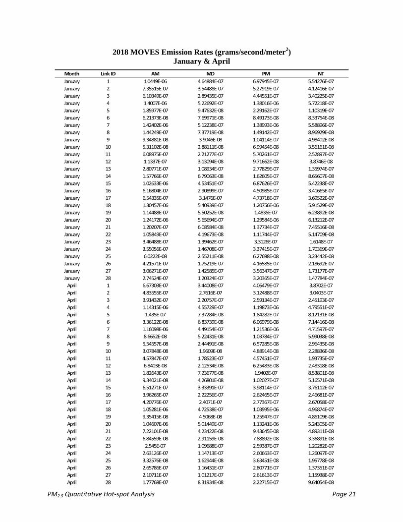
The results of the four hours were extrapolated to cover the entire day. The MOVES2AERMOD tool downloaded from the EPA website was utilized to post‐process MOVES outputs for generating the “EMISFACT” portion of an AERMOD input file. The emission rates as input to AERMOD are in units of grams per second per square meter. Attachment C summarizes MOVES emission rates by four representative time periods for each of the four representative months. A checklist summarizing MOVES “Run Spec” and input assumptions is shown in Attachment D. G.(Step4)RoadDust,Construction,andAdditionalSources Road dust emissions were not included in the analysis as described in Step 2. Construction emissions were not included as the period of construction for this segment will be for less than five years. No additional sources of PM2.5 emissions were included in this analysis. It is assumed that PM2.5 concentrations due to any nearby emissions sources are included in the ambient monitor values that are used as background concentrations. In addition, this project is not expected to result in changes to emissions from existing nearby sources or support any new facilities that would impact localized PM2 5 emissions
H.(Step5)Air‐QualityModel,DataInputs,andReceptorsThe following provides an overview of the air quality modeling undertaken including the assumptions used in EPA’s AERMOD model that was used to estimate concentrations of PM2.5. The AERMOD model requires the determination of the emission sources (e.g. the roadway) and the locations to measure air quality concentrations (e.g. the receptors). Exhibit 4 illustrates the extents used to define the source and receptor locations.
Exhibit 4: Extent of Emissions and Air Quality Modeling

PM2.5 Quantitative Hot‐spot Analysis Page 8
Defined areas were used to delineate the emission sources. Using GIS software, polygons were created having the same roadway segmentation as found in the traffic forecasting and MOVES modeling, with the width set to the width of the travel lanes. The areas/polygons representing ramps include an additional one‐lane wide section parallel the mainline roadway to represent the merge areas. As recommended in the EPA PM hot‐spot guidance, receptors were placed in order to estimate the highest concentrations of PM2.5 and to determine any possible violations of the NAAQS. Areas with higher concentrations of PM2.5 are expected nearest the interchange and along the I‐69 right–of‐way. An area within 5m of the edge of all roadways was excluded as were medians and other areas to which the public would not have access. In cases where it was unclear if the area might be the site for future development, the area was included as a conservative assumption. GIS software was used to define an area within 80 meters of the roadway edges. Within this area (but outside the excluded areas) receptors were located in a 15m grid formation. A second area was then defined between 80m and 500m of the edge of the roadways. Within this area, receptors were located in 75m grid formation. The extensive grid of receptors is used to evaluate the impact of the roadway emissions within the study area. Exhibit 5 illustrates the extent area for receptor locations.
Exhibit 5: Modeled Receptor Locations

PM2.5 Qu
I.(SteThe deteregion. Exhibit 6.
Key refer
T
C
4 Monitor choosing
D
S
Based oconcentr
antitative Hot
p6)Backg
rmination oNo monitor
Exhibi
*Per IDEM,
ences used i
he EPA PM H
onformity ru
0 CFR Part 51
data was othe monitor
istance of m
Wind pattern
imilar charac
n ICG discusations for thi
t‐spot Analysi
groundC
f backgroundis located im
t 6: Monitor
monitor sites
n determining
ot‐spot guida
le, Sections 9
1, Appendix W
btained froms included:
onitor from p
s between mo
teristics betw
sions, the Bs analysis du
*
*
is
oncentrat
emissions wmmediately w
Locations and
2 and 3 are co
g the appropr
ance (Section
3.105(c)(1)(i)
W, Section 8.2
m the EPA’s A
roject area
onitor from p
ween the mon
Bloomingtone to its proxi
tionsfro
was based owithin the st
d Average An
onsidered not a
iate backgro
8)
) and 93.123(c
2.1 and 8.2.3
AIR website
roject area
nitor location
monitor wasimity to the
mNearb
n readings udy area.
nnual PM2.5
appropriate for
und concent
c)
(http://ww
and project a
s selected fstudy area.
yandOthe
available fromNearby monit
Levels Report
r NAAQS comp
ration levels t
w.epa.gov/air
area
or representWith prevailin
P
erSource
m monitors itors are show
ted
parison.
to use include
rdata/). Facto
tative backgrng winds gen
Page 9
es
n the wn in
e:
ors in
round nerally

PM2.5 Quantitative Hot‐spot Analysis Page 10
from the southwest during most of the year (http://iclimate.org/narrative.asp) this appeared to be a conservative choice. The average monitor reading over last 3 years (2010‐2012) was equal to a value
of 10.43 µg/m3; a monitor value that the ICG agreed reasonably reflected the background concentration
in this region. These values are conservative because it is expected that ambient PM2.5 concentrations will be lower in future years as a result of the State Implementation Plan and the general trend in declining vehicle emissions due to technological advances. Also, the project area is decidedly less developed than the areas sampled by these monitors, making the estimated background emissions even more conservative. This value was added to the AERMOD modeled receptor values to yield a design values for comparison to the NAAQS.
J.(Step7)CalculateDesignValuesandDetermineConformity The previous steps of the PM hot‐spot analysis were combined to determine design values that were compared to the NAAQS for each analysis year. The annual PM2 5 design values are defined as the average of three consecutive years’ annual averages, each estimated using equally‐weighted quarterly averages. This NAAQS is met when the three‐year average concentration is less than or equal to the 1997 annual PM2.5 NAAQS. AERMOD was run to provide the annual average PM2.5 concentrations at each receptor. For the receptor with the maximum modeled concentration (in each analysis year), the following steps were used to determine the design value, as outlined in EPA’s guidance.
1. Obtain the average annual concentration for the receptor with the maximum modeled concentration from AERMOD output.
2. Add the average annual background concentration (10.43 µg/m³ as described in Step 6) to the average annual modeled concentration to determine the total average annual concentration.
3. Exhibit 7 summarizes the design values that correspond to the receptor with the maximum modeled concentration for each analysis year. All design values for the maximum receptor location are below the 1997 annual PM2.5 NAAQS of 15.0 µg/m³.
4. It is implied that the design value for all other receptors within the model domain are equal to, or lower than, the values in Exhibit 7, and therefore, are also below the NAAQS.
Exhibit 7: Estimated 2018 and 2035 Design Values
Analysis Year Background
Concentration (µg/m³)
AERMOD Modeling Results*
(µg/m³)
Design Value (µg/m³)
(rounded to one decimal per EPA Guidance)
2018 10.43 0.99 11.4
2035 10.43 0.70 11.1
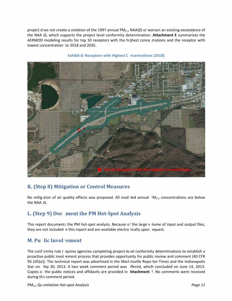
Notes: Modeling results are for the receptors with the maximum concentration. 1997 annual PM2.5 NAAQS is 15 µg/m³ µg/m³ = micrograms per cubic meter AERMOD air quality modeling results show that the annual average concentrations are higher in 2018 than in 2035 as emission rates from MOVES for 2018 are higher than for 2035. Exhibit 8 illustrates the top 10 receptors with the highest concentrations, all of which are from 2018 modeling results. The
PM2.5 Qu
project dthe NAAAERMOD lowest co
K.(Ste No mitigthe NAA
L.(Step This repothey are n
M.Pu The confproactive 93.105(e)Star on Copies oduring th
antitative Hot
oes not creatQS, which supmodeling rencentration
p8)Mitig
ation of air qQS.
p9)Doc
rt documentnot included
blicInvol
ormity rule rpublic invol). The techni
May 30, 2013f the public ne comment p
t‐spot Analysi
e a violation pports the prsults for top for 2018 and
Exhibit 8: R
gationor
uality effects
umentthe
s the PM hotin this report
vement
equires agencvement procecal report wa. A two weeotices and aferiod.
is
of the 1997 aoject level co10 receptors2035.
Receptors wit
ControlM
s was propos
ePMHot‐S
‐spot analysisand are avail
cies completiness that provias advertisedk comment pffidavits are p
annual PM2.5 onformity dets with the hi
th Highest C
Measures
ed. All mod
SpotAnal
s. Because olable electro
ng project‐ledes opportun in the Martperiod was provided in
NAAQS or wotermination.ghest conce
oncentrations
eled annual
lysis
f the large vnically upon
vel conformitnity for publiinsville Repooffered, whichAttachment
orsen an existAttachment
ntrations and
s (2018)
PM2.5 concent
olume of inpurequest.
ty determinatc review and rter‐Times anh concluded F. No comme
Pa
ting exceedanE summarizethe receptor
trations are b
ut and output
tions to estabcomment (4
nd the Indianaon June 14, ents were rec
age 11
nce of es the r with
below
t files,
blish a 40 CFR apolis 2013. ceived

PM2.5 Quantitative Hot‐spot Analysis Page 12
N.ConclusionThis technical report has provided a quantitative PM2.5 hot‐spot analysis for the I‐69 Section 5 project in Indiana. The interagency consultation process played an integral role in defining the need, methodology and assumptions for the analysis. The air quality analysis included modeling techniques to estimate project‐specific emission factors from vehicle exhaust and local PM2.5 concentrations due to project operation. Emissions and dispersion modeling techniques were consistent with the EPA quantitative PM hot‐spot analysis guidance, “Transportation Conformity Guidance for Quantitative Hot‐spot Analysis in PM2.5 and PM10 Nonattainment and Maintenance Areas“ (USEPA, 2010) that was released in December, 2010.
The analysis had demonstrated transportation conformity for the project by determining that future design value concentrations for the 2018 and 2035 analysis year will be lower than the 1997 annual PM2 5 NAAQS of 15.0 µg/m³. As a result, the project does not create a violation of the 1997 annual PM2 5 NAAQS, worsen an existing violation of the NAAQS, or delay timely attainment of the NAAQS and interim milestones, which meets 40 CRF 93.116 and 93.123 and supports the project level conformity determination.
References
“I‐69 Evansville to Indianapolis, Indiana, Section 5, Bloomington to Martinsville, Indiana Tier 2 Final Environmental Impact Statement”
United States Environmental Protection Agency (USEPA). 2010. “Transportation Conformity Guidance for Quantitative Hot‐spot Analyses in PM2.5 and PM10 Nonattainment and Maintenance Areas.”
United States Environmental Protection Agency (USEPA) and United States Department of Transportation. 2012. “Completing Quantitative PM Hot‐spot Analysis: 3 Day Course”
Attachments
Attachment A: I‐69 Section 5 Traffic Volumes
Attachment B: MOVES Link Data Input Files
Attachment C: MOVES Outputs (Emission Rates for AERMOD Modeling) Attachment D: MOVES and AERMOD Input Data Assumptions and Parameters Attachment E: AERMOD Outputs for Top 10 and Lowest Receptors Attachment F: Public Comment Notices and Affidavits

PM2.5 Qu
AttachmI‐69 Se
antitative Hot
ment A: ction 5 Tra
t‐spot Analysi
ffic Volum
is
mes
Paage 13

PM2.5 Quantitative Hot‐spot Analysis Page 14
Attachment B: MOVES Link Data Input Files
MOVES Emissions Analysis Inputs 2018 Daily (For Hours 12 AM and 12 PM Runs)
link ID Road Type ID link Length(miles)
Link Volume(veh/hour)
Link Avg Speed (mph)
Link Description Link Avg Grade
1 4 0.77 674 75.74 55‐I‐069 AB Link 0.05
2 4 0.23 536 76.67 55‐I‐069 AB Link 0.66
3 4 0.94 552 78.33 55‐I‐069 AB Link ‐0.12
4 4 0.26 185 31.84 55‐R‐Flare Ramp AB Link ‐0.15
5 4 0.22 55 34.74 55‐R‐Flare Ramp AB Link ‐0.17
6 4 0.12 19 28.8 55‐R‐Loop Ramp AB Link 1.58
7 4 0.05 158 30 55‐R‐Flare Ramp AB Link 0.76
8 5 0.05 21 8.82 55‐CR‐150 S AB Link 0
9 5 0.04 23 34.29 55‐LS‐ROGERS RD AB Link 0.95
10 4 0.21 25 34.05 55‐R‐Flare Ramp AB Link ‐0.54
11 5 0.19 206 49.57 55‐S‐039‐0‐01 AB Link 0.4
12 5 0.04 9 7.27 55‐LS‐BURTON LN AB Link 0
13 5 0.13 71 39 55‐LS‐BURTON LN AB Link 0
14 5 0.26 47 35.45 55‐LS‐SOUTH VIEW D AB Link 0
15 4 0.93 674 76.44 55‐I‐069 BA Link ‐0.04
16 4 0.58 546 77.33 55‐I‐069 BA Link ‐0.13
17 4 0.55 559 76.74 55‐I‐069 BA Link 0.07
18 4 0.22 180 32.2 55‐R‐Flare Ramp BA Link 0.17
19 4 0.05 29 33.33 55‐R‐Flare Ramp BA Link ‐0.76
20 4 0.36 175 27.69 55‐S‐039‐0‐01 BA Link 0
21 5 0.05 18 8.82 55‐CR‐150 S BA Link 0
22 5 0.06 28 32.73 55‐LS‐ROGERS RD BA Link ‐1.26
23 5 0.19 162 49.57 55‐S‐039‐0‐01 BA Link ‐0.4
24 5 0.08 177 53.33 55‐S‐039‐0‐01 BA Link ‐0.47
25 5 0.04 17 34.29 55‐LS‐BURTON LN BA Link 0
26 5 0.13 70 16.96 55‐LS‐BURTON LN BA Link 0
27 5 0.26 60 22.29 55‐LS‐SOUTH VIEW D BA Link 0
28 5 0.02 23 4 55‐LS‐ROGERS RD AB Link 1.89

PM2.5 Quantitative Hot‐spot Analysis Page 15
MOVES Emissions Analysis Inputs 2018 AM Peak Period (For Hour 6 AM Run)
link ID Road Type ID link Length(miles)
Link Volume(veh/hour)
Link Avg Speed (mph)
Link Description Link Avg Grade
1 4 0.77 1324 75.74 55‐I‐069 AB Link 0.05
2 4 0.23 1064 76.67 55‐I‐069 AB Link 0.66
3 4 0.94 1086 78.33 55‐I‐069 AB Link ‐0.12
4 4 0.26 459 31.84 55‐R‐Flare Ramp AB Link ‐0.15
5 4 0.22 74 34.74 55‐R‐Flare Ramp AB Link ‐0.17
6 4 0.12 37 28.8 55‐R‐Loop Ramp AB Link 1.58
7 4 0.05 423 30 55‐R‐Flare Ramp AB Link 0.76
8 5 0.05 36 8.82 55‐CR‐150 S AB Link 0
9 5 0.04 39 34.29 55‐LS‐ROGERS RD AB Link 0.95
10 4 0.21 39 34.05 55‐R‐Flare Ramp AB Link ‐0.54
11 5 0.19 473 49.57 55‐S‐039‐0‐01 AB Link 0.4
12 5 0.04 26 7.27 55‐LS‐BURTON LN AB Link 0
13 5 0.13 125 39 55‐LS‐BURTON LN AB Link 0
14 5 0.26 78 35.45 55‐LS‐SOUTH VIEW D AB Link 0
15 4 0.93 1324 76.44 55‐I‐069 BA Link ‐0.04
16 4 0.58 1082 77.33 55‐I‐069 BA Link ‐0.13
17 4 0.55 1089 76.74 55‐I‐069 BA Link 0.07
18 4 0.22 424 32.2 55‐R‐Flare Ramp BA Link 0.17
19 4 0.05 41 33.33 55‐R‐Flare Ramp BA Link ‐0.76
20 4 0.36 346 27.69 55‐S‐039‐0‐01 BA Link 0
21 5 0.05 30 8.82 55‐CR‐150 S BA Link 0
22 5 0.06 53 32.73 55‐LS‐ROGERS RD BA Link ‐1.26
23 5 0.19 326 49.57 55‐S‐039‐0‐01 BA Link ‐0.4
24 5 0.08 334 53.33 55‐S‐039‐0‐01 BA Link ‐0.47
25 5 0.04 32 34.29 55‐LS‐BURTON LN BA Link 0
26 5 0.13 121 16.96 55‐LS‐BURTON LN BA Link 0
27 5 0.26 91 22.29 55‐LS‐SOUTH VIEW D BA Link 0
28 5 0.02 39 4 55‐LS‐ROGERS RD AB Link 1.89

PM2.5 Quantitative Hot‐spot Analysis Page 16
MOVES Emissions Analysis Inputs 2018 PM Peak Period (For Hour 6 PM Run)
link ID Road Type ID link Length(miles)
Link Volume(veh/hour)
Link Avg Speed (mph)
Link Description Link Avg Grade
1 4 0.77 1467 75.74 55‐I‐069 AB Link 0.05
2 4 0.23 1298 76.67 55‐I‐069 AB Link 0.66
3 4 0.94 1316 78.33 55‐I‐069 AB Link ‐0.12
4 4 0.26 488 31.84 55‐R‐Flare Ramp AB Link ‐0.15
5 4 0.22 116 34.74 55‐R‐Flare Ramp AB Link ‐0.17
6 4 0.12 48 28.8 55‐R‐Loop Ramp AB Link 1.58
7 4 0.05 426 30 55‐R‐Flare Ramp AB Link 0.76
8 5 0.05 43 8.82 55‐CR‐150 S AB Link 0
9 5 0.04 59 34.29 55‐LS‐ROGERS RD AB Link 0.95
10 4 0.21 56 34.05 55‐R‐Flare Ramp AB Link ‐0.54
11 5 0.19 529 49.57 55‐S‐039‐0‐01 AB Link 0.4
12 5 0.04 30 7.27 55‐LS‐BURTON LN AB Link 0
13 5 0.13 160 39 55‐LS‐BURTON LN AB Link 0
14 5 0.26 110 35.45 55‐LS‐SOUTH VIEW D AB Link 0
15 4 0.93 1467 76.44 55‐I‐069 BA Link ‐0.04
16 4 0.58 1322 77.33 55‐I‐069 BA Link ‐0.13
17 4 0.55 1311 76.74 55‐I‐069 BA Link 0.07
18 4 0.22 426 32.2 55‐R‐Flare Ramp BA Link 0.17
19 4 0.05 65 33.33 55‐R‐Flare Ramp BA Link ‐0.76
20 4 0.36 429 27.69 55‐S‐039‐0‐01 BA Link 0
21 5 0.05 41 8.82 55‐CR‐150 S BA Link 0
22 5 0.06 70 32.73 55‐LS‐ROGERS RD BA Link ‐1.26
23 5 0.19 381 49.57 55‐S‐039‐0‐01 BA Link ‐0.4
24 5 0.08 412 53.33 55‐S‐039‐0‐01 BA Link ‐0.47
25 5 0.04 47 34.29 55‐LS‐BURTON LN BA Link 0
26 5 0.13 158 16.96 55‐LS‐BURTON LN BA Link 0
27 5 0.26 135 22.29 55‐LS‐SOUTH VIEW D BA Link 0
28 5 0.02 59 4 55‐LS‐ROGERS RD AB Link 1.89

PM2.5 Quantitative Hot‐spot Analysis Page 17
MOVES Emissions Analysis Inputs 2035 Daily (For Hours 12 AM and 12 PM Runs)
link ID Road Type ID link Length(miles)
Link Volume(veh/hour)
Link Avg Speed (mph)
Link Description Link Avg Grade
1 4 0.77 1295 75.74 55‐I‐069 AB Link 0.05
2 4 0.23 1036 76.67 55‐I‐069 AB Link 0.66
3 4 0.94 1115 78.33 55‐I‐069 AB Link ‐0.12
4 4 0.26 259 31.84 55‐R‐Flare Ramp AB Link ‐0.15
5 4 0.22 79 34.74 55‐R‐Flare Ramp AB Link ‐0.17
6 4 0.12 79 28.8 55‐R‐Loop Ramp AB Link 1.58
7 4 0.05 324 30 55‐R‐Flare Ramp AB Link 0.76
8 5 0.05 23 8.82 55‐CR‐150 S AB Link 0
9 5 0.04 29 34.29 55‐LS‐ROGERS RD AB Link 0.95
10 4 0.21 87 34.05 55‐R‐Flare Ramp AB Link ‐0.54
11 5 0.19 311 49.57 55‐S‐039‐0‐01 AB Link 0.4
12 5 0.04 11 7.27 55‐LS‐BURTON LN AB Link 0
13 5 0.13 56 39 55‐LS‐BURTON LN AB Link 0
14 5 0.26 43 35.45 55‐LS‐SOUTH VIEW D AB Link 0
15 4 0.93 1281 76.44 55‐I‐069 BA Link ‐0.04
16 4 0.58 1086 77.33 55‐I‐069 BA Link ‐0.13
17 4 0.55 1174 76.74 55‐I‐069 BA Link 0.07
18 4 0.22 259 32.2 55‐R‐Flare Ramp BA Link 0.17
19 4 0.05 59 33.33 55‐R‐Flare Ramp BA Link ‐0.76
20 4 0.36 194 27.69 55‐S‐039‐0‐01 BA Link 0
21 5 0.05 20 8.82 55‐CR‐150 S BA Link 0
22 5 0.06 36 32.73 55‐LS‐ROGERS RD BA Link ‐1.26
23 5 0.19 245 49.57 55‐S‐039‐0‐01 BA Link ‐0.4
24 5 0.08 198 53.33 55‐S‐039‐0‐01 BA Link ‐0.47
25 5 0.04 22 34.29 55‐LS‐BURTON LN BA Link 0
26 5 0.13 55 16.96 55‐LS‐BURTON LN BA Link 0
27 5 0.26 55 22.29 55‐LS‐SOUTH VIEW D BA Link 0
28 5 0.02 29 4 55‐LS‐ROGERS RD AB Link 1.89

PM2.5 Quantitative Hot‐spot Analysis Page 18
MOVES Emissions Analysis Inputs 2035 AM Peak Period (For Hour 6 AM Run)
link ID Road Type ID link Length(miles)
Link Volume(veh/hour)
Link Avg Speed (mph)
Link Description Link Avg Grade
1 4 0.77 2549 75.74 55‐I‐069 AB Link 0.05
2 4 0.23 2018 76.67 55‐I‐069 AB Link 0.66
3 4 0.94 2110 78.33 55‐I‐069 AB Link ‐0.12
4 4 0.26 531 31.84 55‐R‐Flare Ramp AB Link ‐0.15
5 4 0.22 92 34.74 55‐R‐Flare Ramp AB Link ‐0.17
6 4 0.12 92 28.8 55‐R‐Loop Ramp AB Link 1.58
7 4 0.05 646 30 55‐R‐Flare Ramp AB Link 0.76
8 5 0.05 36 8.82 55‐CR‐150 S AB Link 0
9 5 0.04 42 34.29 55‐LS‐ROGERS RD AB Link 0.95
10 4 0.21 151 34.05 55‐R‐Flare Ramp AB Link ‐0.54
11 5 0.19 626 49.57 55‐S‐039‐0‐01 AB Link 0.4
12 5 0.04 27 7.27 55‐LS‐BURTON LN AB Link 0
13 5 0.13 76 39 55‐LS‐BURTON LN AB Link 0
14 5 0.26 53 35.45 55‐LS‐SOUTH VIEW D AB Link 0
15 4 0.93 2249 76.44 55‐I‐069 BA Link ‐0.04
16 4 0.58 1869 77.33 55‐I‐069 BA Link ‐0.13
17 4 0.55 2020 76.74 55‐I‐069 BA Link 0.07
18 4 0.22 531 32.2 55‐R‐Flare Ramp BA Link 0.17
19 4 0.05 63 33.33 55‐R‐Flare Ramp BA Link ‐0.76
20 4 0.36 380 27.69 55‐S‐039‐0‐01 BA Link 0
21 5 0.05 29 8.82 55‐CR‐150 S BA Link 0
22 5 0.06 57 32.73 55‐LS‐ROGERS RD BA Link ‐1.26
23 5 0.19 431 49.57 55‐S‐039‐0‐01 BA Link ‐0.4
24 5 0.08 389 53.33 55‐S‐039‐0‐01 BA Link ‐0.47
25 5 0.04 33 34.29 55‐LS‐BURTON LN BA Link 0
26 5 0.13 74 16.96 55‐LS‐BURTON LN BA Link 0
27 5 0.26 63 22.29 55‐LS‐SOUTH VIEW D BA Link 0
28 5 0.02 42 4 55‐LS‐ROGERS RD AB Link 1.89

PM2.5 Quantitative Hot‐spot Analysis Page 19
MOVES Emissions Analysis Inputs 2035 PM Peak Period (For Hour 6 PM Run)
link ID Road Type ID link Length(miles)
Link Volume(veh/hour)
Link Avg Speed (mph)
Link Description Link Avg Grade
1 4 0.77 2801 75.74 55‐I‐069 AB Link 0.05
2 4 0.23 2160 76.67 55‐I‐069 AB Link 0.66
3 4 0.94 2334 78.33 55‐I‐069 AB Link ‐0.12
4 4 0.26 641 31.84 55‐R‐Flare Ramp AB Link ‐0.15
5 4 0.22 174 34.74 55‐R‐Flare Ramp AB Link ‐0.17
6 4 0.12 174 28.8 55‐R‐Loop Ramp AB Link 1.58
7 4 0.05 794 30 55‐R‐Flare Ramp AB Link 0.76
8 5 0.05 55 8.82 55‐CR‐150 S AB Link 0
9 5 0.04 75 34.29 55‐LS‐ROGERS RD AB Link 0.95
10 4 0.21 208 34.05 55‐R‐Flare Ramp AB Link ‐0.54
11 5 0.19 761 49.57 55‐S‐039‐0‐01 AB Link 0.4
12 5 0.04 37 7.27 55‐LS‐BURTON LN AB Link 0
13 5 0.13 127 39 55‐LS‐BURTON LN AB Link 0
14 5 0.26 94 35.45 55‐LS‐SOUTH VIEW D AB Link 0
15 4 0.93 2668 76.44 55‐I‐069 BA Link ‐0.04
16 4 0.58 2220 77.33 55‐I‐069 BA Link ‐0.13
17 4 0.55 2428 76.74 55‐I‐069 BA Link 0.07
18 4 0.22 641 32.2 55‐R‐Flare Ramp BA Link 0.17
19 4 0.05 122 33.33 55‐R‐Flare Ramp BA Link ‐0.76
20 4 0.36 448 27.69 55‐S‐039‐0‐01 BA Link 0
21 5 0.05 52 8.82 55‐CR‐150 S BA Link 0
22 5 0.06 89 32.73 55‐LS‐ROGERS RD BA Link ‐1.26
23 5 0.19 548 49.57 55‐S‐039‐0‐01 BA Link ‐0.4
24 5 0.08 459 53.33 55‐S‐039‐0‐01 BA Link ‐0.47
25 5 0.04 57 34.29 55‐LS‐BURTON LN BA Link 0
26 5 0.13 126 16.96 55‐LS‐BURTON LN BA Link 0
27 5 0.26 116 22.29 55‐LS‐SOUTH VIEW D BA Link 0
28 5 0.02 75 4 55‐LS‐ROGERS RD AB Link 1.89

PM2.5 Quantitative Hot‐spot Analysis Page 20
Attachment C: MOVES Outputs (Emission Rates for AERMOD Modeling)
<Data Outputs Begin on Following Page>
PM2.5 Quantitative Hot‐spot Analysis Page 21
2018 MOVES Emission Rates (grams/second/meter2) January & April
Month Link ID AM MD PM NTJanuary 1 1.0449E‐06 4.64884E‐07 6.97945E‐07 5.54276E‐07
January 2 7.35515E‐07 3.54488E‐07 5.27919E‐07 4.12416E‐07
January 3 6.10349E‐07 2.89435E‐07 4.44551E‐07 3.40225E‐07
January 4 1.4007E‐06 5.22692E‐07 1.38016E‐06 5.72218E‐07
January 5 1.85977E‐07 9.47632E‐08 2.29162E‐07 1.10319E‐07
January 6 6.21373E‐08 7.69971E‐08 8.49173E‐08 8.33754E‐08
January 7 1.42402E‐06 5.12238E‐07 1.38993E‐06 5.58896E‐07
January 8 1.44249E‐07 7.37719E‐08 1.49142E‐07 8.96929E‐08
January 9 9.34881E‐08 3.9046E‐08 1.04114E‐07 4.98402E‐08
January 10 5.31102E‐08 2.88111E‐08 6.99454E‐08 3.56161E‐08
January 11 6.08975E‐07 2.21277E‐07 5.70261E‐07 2.52897E‐07
January 12 1.1337E‐07 3.13094E‐08 9.71662E‐08 3.8746E‐08
January 13 2.80771E‐07 1.08934E‐07 2.77829E‐07 1.35974E‐07
January 14 1.57766E‐07 6.79063E‐08 1.62605E‐07 8.65607E‐08
January 15 1.02633E‐06 4.53451E‐07 6.87626E‐07 5.42238E‐07
January 16 6.16804E‐07 2.90899E‐07 4.50985E‐07 3.41665E‐07
January 17 6.54335E‐07 3.1476E‐07 4.73718E‐07 3.69522E‐07
January 18 1.30457E‐06 5.40939E‐07 1.20756E‐06 5.91529E‐07
January 19 1.14488E‐07 5.50252E‐08 1.4835E‐07 6.23892E‐08
January 20 1.24172E‐06 5.65694E‐07 1.29584E‐06 6.13212E‐07
January 21 1.20207E‐07 6.08584E‐08 137734E‐07 7.45516E‐08
January 22 1.05849E‐07 4.19673E‐08 1.11744E‐07 5.14709E‐08
January 23 3.46488E‐07 1.39462E‐07 3.3126E‐07 1.6148E‐07
January 24 3.55056E‐07 1.46708E‐07 3.37415E‐07 1.70369E‐07
January 25 6.0222E‐08 2.55211E‐08 6.27698E‐08 3.23442E‐08
January 26 4.21571E‐07 1.75219E‐07 4.16585E‐07 2.18692E‐07
January 27 3.06271E‐07 1.42585E‐07 3.56347E‐07 1.73177E‐07
January 28 2.74524E‐07 1.20324E‐07 3.20365E‐07 1.47784E‐07
April 1 6.67303E‐07 3.44008E‐07 4.06479E‐07 3.8702E‐07
April 2 4.83555E‐07 2.7616E‐07 3.12488E‐07 3.0403E‐07
April 3 3.91432E‐07 2.20757E‐07 2.59134E‐07 2.45193E‐07
April 4 1.14315E‐06 4.55729E‐07 1.19873E‐06 4.79551E‐07
April 5 1.435E‐07 7.37284E‐08 1.84282E‐07 8.12131E‐08
April 6 3.36122E‐08 6.83739E‐08 6.06979E‐08 7.14416E‐08
April 7 1.16098E‐06 4.49154E‐07 1.21536E‐06 4.71597E‐07
April 8 8.6652E‐08 5.22431E‐08 1.03784E‐07 5.99038E‐08
April 9 5.54557E‐08 2.44491E‐08 6.57285E‐08 2.96435E‐08
April 10 3.07848E‐08 1.9609E‐08 4.88914E‐08 2.28836E‐08
April 11 4.57847E‐07 1.78523E‐07 4.57451E‐07 1.93735E‐07
April 12 6.8403E‐08 2.12534E‐08 6.25483E‐08 2.48318E‐08
April 13 1.82643E‐07 7.23677E‐08 1.9402E‐07 8.53801E‐08
April 14 9.34021E‐08 4.26801E‐08 1.02027E‐07 5.16571E‐08
April 15 6.51271E‐07 3.33391E‐07 3.98114E‐07 3.76112E‐07
April 16 3.96265E‐07 2.22256E‐07 2.62465E‐07 2.46681E‐07
April 17 4.20776E‐07 2.4071E‐07 2.77367E‐07 2.67058E‐07
April 18 1.05281E‐06 4.72538E‐07 1.03995E‐06 4.96874E‐07
April 19 9.35415E‐08 45068E‐08 1.25947E‐07 4.86109E‐08
April 20 1.04607E‐06 5.01449E‐07 1.13241E‐06 5.24305E‐07
April 21 7.22101E‐08 4.23422E‐08 9.43645E‐08 4.89311E‐08
April 22 6.84559E‐08 2.91159E‐08 7.88892E‐08 3.36891E‐08
April 23 2.545E‐07 1.09688E‐07 2.59387E‐07 1.20282E‐07
April 24 2.63126E‐07 1.14713E‐07 2.60663E‐07 1.26097E‐07
April 25 3.32576E‐08 1.62944E‐08 3.63451E‐08 1.95778E‐08
April 26 2.65786E‐07 1.16431E‐07 2.80771E‐07 1.37351E‐07
April 27 2.10711E‐07 1.01217E‐07 2.61613E‐07 1.15938E‐07
April 28 1.77768E‐07 8.31934E‐08 2.22715E‐07 9.64054E‐08

PM2.5 Quantitative Hot‐spot Analysis Page 22
2018 MOVES Emission Rates (grams/second/meter2) July & October
Month MOVESlinkID AM MD PM NTJuly 1 5.95063E‐07 3.39754E‐07 3.89155E‐07 356384E‐07
July 2 4.35351E‐07 2.7341E‐07 2.99683E‐07 2.84178E‐07
July 3 3.4955E‐07 2.18343E‐07 2.48112E‐07 2.27787E‐07
July 4 1.09388E‐06 4.53392E‐07 1.18804E‐06 4.62581E‐07
July 5 1.35374E‐07 7.29888E‐08 1.81628E‐07 758824E‐08
July 6 2.81551E‐08 6.80736E‐08 5.9261E‐08 6.92562E‐08
July 7 1.11066E‐06 4.46956E‐07 1.20508E‐06 4.5561E‐07
July 8 7.56334E‐08 5.14848E‐08 1.01094E‐07 5.44481E‐08
July 9 4.81797E‐08 2.39329E‐08 6.34476E‐08 259444E‐08
July 10 2.65138E‐08 1.92843E‐08 4.76425E‐08 2.05517E‐08
July 11 4.28934E‐07 1.77023E‐07 4.50784E‐07 1.82898E‐07
July 12 5.98006E‐08 2.08992E‐08 6.04948E‐08 2.22834E‐08
July 13 1.6387E‐07 7.10762E‐08 1.89047E‐07 7.61135E‐08
July 14 8.10886E‐08 4.17884E‐08 9.84277E‐08 452644E‐08
July 15 5.79518E‐07 3.29167E‐07 3.80903E‐07 3.45683E‐07
July 16 3.54073E‐07 2.19843E‐07 2.51259E‐07 2.29282E‐07
July 17 3.76093E‐07 2.38108E‐07 2.65696E‐07 2.4829E‐07
July 18 1.00464E‐06 4.70153E‐07 1.03006E‐06 4.79539E‐07
July 19 8.95344E‐08 4.47188E‐08 1.24626E‐07 4.60874E‐08
July 20 1.00864E‐06 4.99215E‐07 1.12279E‐06 5.08022E‐07
July 21 6.30278E‐08 4.16897E‐08 9.17925E‐08 4.42387E‐08
July 22 6.13023E‐08 2.86622E‐08 7.69393E‐08 3.04325E‐08
July 23 2.36901E‐07 1.08643E‐07 255134E‐07 1.12737E‐07
July 24 2.45539E‐07 1.1359E‐07 256122E‐07 1.17989E‐07
July 25 2.8099E‐08 1.59682E‐08 3.47741E‐08 1.72396E‐08
July 26 2.35982E‐07 1.14354E‐07 2.72706E‐07 1.22453E‐07
July 27 1.92429E‐07 9.97569E‐08 2.55993E‐07 1.05454E‐07
July 28 1.59258E‐07 8.18895E‐08 2.16938E‐07 8.69958E‐08
October 1 8.71803E‐07 4.10616E‐07 5.67415E‐07 4.77657E‐07
October 2 6.20011E‐07 3.1932E‐07 4.31438E‐07 3.62765E‐07
October 3 5.09993E‐07 2.58601E‐07 3.61512E‐07 2.96691E‐07
October 4 1.28264E‐06 4.92626E‐07 1.29891E‐06 5.29771E‐07
October 5 1.66506E‐07 8.53197E‐08 2.09063E‐07 9.69866E‐08
October 6 4.90612E‐08 7.31254E‐08 7.40711E‐08 7.79086E‐08
October 7 1.30344E‐06 4.83915E‐07 131175E‐06 5.18907E‐07
October 8 1.17846E‐07 6.41069E‐08 1.28829E‐07 7.60474E‐08
October 9 7.60535E‐08 3.2493E‐08 8.6924E‐08 4.05885E‐08
October 10 4.28764E‐08 2.46801E‐08 6.05169E‐08 2.97838E‐08
October 11 5.39696E‐07 2.02081E‐07 5.19739E‐07 2.25796E‐07
October 12 9.27569E‐08 2.67949E‐08 8.16636E‐08 3.23723E‐08
October 13 2.35789E‐07 9.25185E‐08 2.40296E‐07 1.12798E‐07
October 14 1.28261E‐07 5.65817E‐08 1.35476E‐07 7.05723E‐08
October 15 8.54392E‐07 3.99549E‐07 5.57968E‐07 4.66136E‐07
October 16 5.15703E‐07 2.60081E‐07 3.66558E‐07 2.98153E‐07
October 17 5.47266E‐07 2.81512E‐07 3.85783E‐07 3.22585E‐07
October 18 1.18916E‐06 5.10229E‐07 1.1325E‐06 5.4817E‐07
October 19 1.04886E‐07 5.05549E‐08 138317E‐07 5.60778E‐08
October 20 1.15203E‐06 5.3685E‐07 1.22265E‐06 5.72487E‐07
October 21 9.82051E‐08 5.2546E‐08 1.18312E‐07 6.28156E‐08
October 22 8.87076E‐08 3.61981E‐08 9.70307E‐08 433256E‐08
October 23 3.04319E‐07 1.26095E‐07 2.99072E‐07 1.42608E‐07
October 24 3.12914E‐07 1.32343E‐07 3.03042E‐07 150089E‐07
October 25 4.78612E‐08 2.13791E‐08 5.09361E‐08 2.64962E‐08
October 26 3.50156E‐07 1.48827E‐07 3.55762E‐07 1.81431E‐07
October 27 2.62465E‐07 1.24013E‐07 3.13921E‐07 1.46957E‐07
October 28 2.30172E‐07 1.03655E‐07 2.76636E‐07 1.2425E‐07

PM2.5 Quantitative Hot‐spot Analysis Page 23
2035 MOVES Emission Rates (grams/second/meter2) January & April
Month Link ID AM MD PM NTJanuary 1 1.21261E‐06 4.2384E‐07 8.76147E‐07 5.57726E‐07
January 2 8.01159E‐07 2.88295E‐07 5.64625E‐07 3.73834E‐07
January 3 7.09373E‐07 2.6038E‐07 5.18629E‐07 3.39648E‐07
January 4 7.22501E‐07 2.66233E‐07 6.26542E‐07 3.30259E‐07
January 5 1.20092E‐07 7.25254E‐08 1.60024E‐07 9.26794E‐08
January 6 1.4445E‐07 853202E‐08 1.87388E‐07 1.10342E‐07
January 7 9.14102E‐07 338989E‐07 7.93906E‐07 4.26287E‐07
January 8 1.32663E‐07 6.21682E‐08 1.48443E‐07 7.7321E‐08
January 9 7.83307E‐08 3.68604E‐08 9.64936E‐08 4.87591E‐08
January 10 1.91124E‐07 7.97971E‐08 1.90857E‐07 1.00548E‐07
January 11 3.83146E‐07 1.29211E‐07 3.13192E‐07 1.72802E‐07
January 12 1.03843E‐07 3.12758E‐08 1.05099E‐07 3.92891E‐08
January 13 1.17988E‐07 5.96745E‐08 1.37228E‐07 7.85002E‐08
January 14 8.62894E‐08 4.85519E‐08 1.07812E‐07 6.36153E‐08
January 15 1.05973E‐06 4.15093E‐07 8.30292E‐07 5.46144E‐07
January 16 6.34824E‐07 257729E‐07 5.00383E‐07 3.34974E‐07
January 17 7.22548E‐07 2.91088E‐07 5.73846E‐07 3.80811E‐07
January 18 7.26854E‐07 2.6474E‐07 6.22888E‐07 3.3133E‐07
January 19 8.2266E‐08 552775E‐08 1.13894E‐07 6.8978E‐08
January 20 5.46102E‐07 2.13526E‐07 4.70333E‐07 2.62659E‐07
January 21 1.06112E‐07 532902E‐08 1.39049E‐07 6.65173E‐08
January 22 9.27493E‐08 4.25893E‐08 1.06205E‐07 5.35399E‐08
January 23 2.39251E‐07 9.33032E‐08 2.07321E‐07 1.23642E‐07
January 24 2.07255E‐07 7.1458E‐08 1.65149E‐07 9.58045E‐08
January 25 5.53079E‐08 2.58081E‐08 6.75275E‐08 3.35828E‐08
January 26 1.94695E‐07 1.03494E‐07 2.39617E‐07 1.32303E‐07
January 27 1.44014E‐07 8.94737E‐08 1.90927E‐07 1.13872E‐07
January 28 2.31109E‐07 1.13151E‐07 2.92916E‐07 1.44416E‐07
April 1 6.18235E‐07 2.4282E‐07 4.0036E‐07 3.07218E‐07
April 2 4.17383E‐07 1.72649E‐07 2.59414E‐07 2.13785E‐07
April 3 3.68495E‐07 1.53206E‐07 2.39406E‐07 1.91332E‐07
April 4 4.47505E‐07 1.79659E‐07 4.01453E‐07 2.10463E‐07
April 5 7.18988E‐08 452724E‐08 9.79867E‐08 5.49701E‐08
April 6 8.46285E‐08 5.14846E‐08 1.10356E‐07 6.35246E‐08
April 7 5.50398E‐07 2.20949E‐07 4.91008E‐07 2.6295E‐07
April 8 8.36091E‐08 4.16784E‐08 9.79072E‐08 4.89693E‐08
April 9 4.26616E‐08 2.07699E‐08 5.35826E‐08 2.64959E‐08
April 10 1.16548E‐07 5.17372E‐08 1.21532E‐07 6.17219E‐08
April 11 1.99715E‐07 7.02664E‐08 1.62085E‐07 9.1241E‐08
April 12 6.28016E‐08 2.044E‐08 6.75088E‐08 2.42958E‐08
April 13 6.509E‐08 3.42171E‐08 7.77445E‐08 4.32764E‐08
April 14 4.77233E‐08 2.81817E‐08 6.20046E‐08 3.54307E‐08
April 15 5.49068E‐07 237907E‐07 3.81224E‐07 3.00941E‐07
April 16 3.37283E‐07 153294E‐07 2.32866E‐07 1.90444E‐07
April 17 3.79339E‐07 1.6978E‐07 2.64451E‐07 2.12934E‐07
April 18 4.40845E‐07 1.747E‐07 3.88778E‐07 2.06737E‐07
April 19 5.23491E‐08 3.67513E‐08 7.42895E‐08 4.33435E‐08
April 20 3.44305E‐07 1.47089E‐07 3.09568E‐07 1.70728E‐07
April 21 6.6474E‐08 3.54044E‐08 9.113E‐08 4.17687E‐08
April 22 5.68605E‐08 2.7781E‐08 6.85159E‐08 3.30506E‐08
April 23 1.27854E‐07 5.22786E‐08 1.11508E‐07 6.68769E‐08
April 24 1.07059E‐07 3.85358E‐08 8.53048E‐08 5.02511E‐08
April 25 3.10804E‐08 152946E‐08 3.94501E‐08 1.90359E‐08
April 26 1.14175E‐07 6.45364E‐08 1.47736E‐07 7.83997E‐08
April 27 8.63492E‐08 5.6481E‐08 1.19281E‐07 6.82218E‐08
April 28 1.37367E‐07 7.08769E‐08 1.80193E‐07 8.59189E‐08

PM2.5 Quantitative Hot‐spot Analysis Page 24
2035 MOVES Emission Rates (grams/second/meter2) July & October
Month MOVESlinkID AM MD PM NTJuly 1 5.04522E‐07 2.36516E‐07 3.721E‐07 2.61335E‐07
July 2 3.4396E‐07 1.68645E‐07 2.41292E‐07 1.84471E‐07
July 3 3.03279E‐07 1.49482E‐07 2.22824E‐07 1.64166E‐07
July 4 3.94896E‐07 1.76621E‐07 3.88109E‐07 1.88523E‐07
July 5 6.26792E‐08 4.43117E‐08 9.43054E‐08 4.80638E‐08
July 6 7.31844E‐08 5.02925E‐08 1.05786E‐07 5.49499E‐08
July 7 4.8082E‐07 2.16808E‐07 4.73055E‐07 2.33036E‐07
July 8 7.42249E‐08 4.09571E‐08 9.49112E‐08 4.37767E‐08
July 9 3.58377E‐08 2.02011E‐08 5.10321E‐08 2.24182E‐08
July 10 1.02281E‐07 5.07487E‐08 1.1742E‐07 5.46111E‐08
July 11 1.64622E‐07 6.81893E‐08 1.53112E‐07 7.63028E‐08
July 12 5.49501E‐08 2.00582E‐08 6.5279E‐08 2.15498E‐08
July 13 5.497E‐08 3.33173E‐08 7.42098E‐08 3.6825E‐08
July 14 4.03451E‐08 2.74612E‐08 5.92818E‐08 3.02686E‐08
July 15 4.51369E‐07 2.31736E‐07 3.54552E‐07 2.5603E‐07
July 16 2.80358E‐07 1.49669E‐07 2.16983E‐07 1.63972E‐07
July 17 3.13679E‐07 1.65564E‐07 2.46077E‐07 1.82185E‐07
July 18 3.86129E‐07 1.7154E‐07 3.74898E‐07 1.83918E‐07
July 19 4.66258E‐08 3.60991E‐08 7.19409E‐08 3.86486E‐08
July 20 3.057E‐07 1.44758E‐07 3.00039E‐07 1.53891E‐07
July 21 5.8891E‐08 3.47743E‐08 8.82884E‐08 3.72361E‐08
July 22 4.99946E‐08 2.72582E‐08 6.62778E‐08 2.92979E‐08
July 23 1.06542E‐07 5.08322E‐08 1.05818E‐07 5.64802E‐08
July 24 8.78906E‐08 3.73746E‐08 8.05617E‐08 4.19077E‐08
July 25 2.64455E‐08 1.49229E‐08 3.77814E‐08 1.63716E‐08
July 26 9.87708E‐08 6.31596E‐08 1.42277E‐07 6.8527E‐08
July 27 7.5317E‐08 5.53156E‐08 1.15025E‐07 5.98606E‐08
July 28 1.19434E‐07 6.93922E‐08 1.73519E‐07 7.52056E‐08
October 1 9.40131E‐07 3.42558E‐07 6.63065E‐07 4.4297E‐07
October 2 6.25224E‐07 2.36365E‐07 4.27935E‐07 3.00517E‐07
October 3 5.53107E‐07 2.12256E‐07 3.93578E‐07 2.71706E‐07
October 4 5.96441E‐07 2.27366E‐07 5.25741E‐07 2.75384E‐07
October 5 9.80001E‐08 6.02905E‐08 1.32242E‐07 7.54057E‐08
October 6 1.17027E‐07 7.01302E‐08 1.52891E‐07 8.88963E‐08
October 7 7.47379E‐07 2.85996E‐07 6.5826E‐07 3.51467E‐07
October 8 1.10176E‐07 5.29696E‐08 1.25811E‐07 6.43339E‐08
October 9 6.19795E‐08 2.96368E‐08 7.72765E‐08 3.85606E‐08
October 10 1.56938E‐07 6.72001E‐08 1.59812E‐07 8.27629E‐08
October 11 2.99058E‐07 1.02748E‐07 2.45521E‐07 1.3544E‐07
October 12 8.50295E‐08 2.64113E‐08 8.82653E‐08 3.24211E‐08
October 13 9.37392E‐08 4.82461E‐08 1.10589E‐07 6.23648E‐08
October 14 6.86102E‐08 3.94072E‐08 8.7298E‐08 5.07044E‐08
October 15 8.25629E‐07 3.35534E‐07 6.29176E‐07 4.33819E‐07
October 16 4.98424E‐07 2.10834E‐07 3.80575E‐07 2.68765E‐07
October 17 5.65213E‐07 2.36617E‐07 4.35283E‐07 3.03906E‐07
October 18 5.95746E‐07 2.24317E‐07 5.18047E‐07 2.74257E‐07
October 19 6.85519E‐08 4.69604E‐08 9.61579E‐08 5.72356E‐08
October 20 4.53597E‐07 1.83699E‐07 3.98338E‐07 2.20549E‐07
October 21 8.79416E‐08 4.52605E‐08 1.17589E‐07 5.51806E‐08
October 22 7.62974E‐08 3.59414E‐08 8.93268E‐08 4.41542E‐08
October 23 1.88185E‐07 7.48857E‐08 1.64413E‐07 9.76388E‐08
October 24 1.61324E‐07 5.6678E‐08 1.29393E‐07 7.49373E‐08
October 25 4.42017E‐08 2.10883E‐08 5.49537E‐08 2.69191E‐08
October 26 1.57783E‐07 8.60046E‐08 1.98469E‐07 1.07611E‐07
October 27 1.1758E‐07 7.46624E‐08 1.58841E‐07 9.29602E‐08
October 28 1.88138E‐07 9.41728E‐08 2.42436E‐07 1.1762E‐07
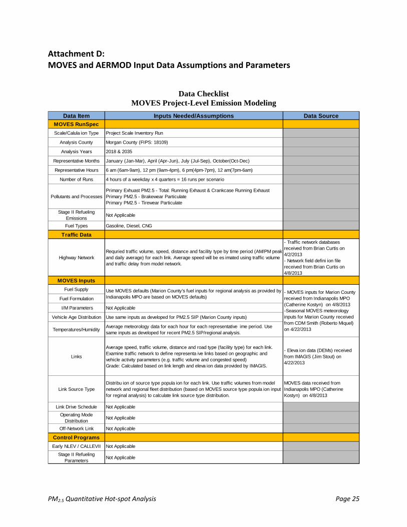
PM2.5 Quantitative Hot‐spot Analysis Page 25
Attachment D: MOVES and AERMOD Input Data Assumptions and Parameters
Data Checklist MOVES Project-Level Emission Modeling
Data Item Inputs Needed/Assumptions Data SourceMOVES RunSpec
Scale/Calula ion Type Project Scale Inventory Run
Analysis County Morgan County (FIPS: 18109)
Analysis Years 2018 & 2035
Representative Months January (Jan-Mar), April (Apr-Jun), July (Jul-Sep), October(Oct-Dec)
Representative Hours 6 am (6am-9am), 12 pm (9am-4pm), 6 pm(4pm-7pm), 12 am(7pm-6am)
Number of Runs 4 hours of a weekday x 4 quarters = 16 runs per scenario
Pollutants and ProcessesPrimary Exhuast PM2.5 - Total: Running Exhaust & Crankcase Running ExhaustPrimary PM2.5 - Brakewear ParticulatePrimary PM2.5 - Tirewear Particulate
Stage II Refueling Emissions Not Applicable
Fuel Types Gasoline, Diesel, CNG
Traffic Data
Highway NetworkRequried traffic volume, speed, distance and facility type by time period (AM/PM peak and daily average) for each link. Average speed will be es imated using traffic volume and traffic delay from model network.
- Traffic network databases received from Brian Curtis on 4/2/2013- Network field defini ion file received from Brian Curtis on 4/8/2013
MOVES Inputs
Fuel Supply
Fuel Formulation
I/M Parameters Not Applicable
Vehicle Age Distribution Use same inputs as developed for PM2.5 SIP (Marion County inputs)
Temperatures/Humidity Average meteorology data for each hour for each representative ime period. Use same inputs as developed for recent PM2.5 SIP/regional analysis.
Links
Average speed, traffic volume, distance and road type (facility type) for each link. Examine traffic network to define representa ive links based on geographic and vehicle activity parameters (e.g. traffic volume and congested speed)Grade: Calculated based on link length and eleva ion data provided by IMAGIS.
- Eleva ion data (DEMs) received from IMAGIS (Jim Stout) on 4/22/2013
Link Source TypeDistribu ion of source type popula ion for each link. Use traffic volumes from model network and regional fleet distribution (based on MOVES source type popula ion input for reginal analysis) to calculate link source type distribution.
MOVES data received from Indianapolis MPO (Catherine Kostyn) on 4/8/2013
Link Drive Schedule Not ApplicableOperating Mode
Distribution Not Applicable
Off-Network Link Not Applicable
Control Programs
Early NLEV / CALLEVII Not Applicable
Stage II Refueling Parameters Not Applicable
- MOVES inputs for Marion County received from Indianapolis MPO (Catherine Kostyn) on 4/8/2013-Seasonal MOVES meteorology inputs for Marion County received from CDM Smith (Roberto Miquel) on 4/22/2013
Use MOVES defaults (Marion County's fuel inputs for regional analysis as provided by Indianapolis MPO are based on MOVES defaults)

PM2.5 Quantitative Hot‐spot Analysis Page 26
Data Checklist AERMOD Dispersion Modeling
Data Item Inputs Needed/Assumptions Data SourceAnalysis
Air Quality Dispersion Model AERMOD (Dated 12345)Downloaded from EPA's SCRAM website(http://www.epa.gov/ttn/scram/dispersion
_prefrec.htm#aermod)
Key AERMOD Inputs
Modeling Options Modle concentration and assume flat terrain
Pollutant PM 2.5
Averaging Period Annual
Receptor Height 1.8 metersPer EPA & DOT “Completing Quantitative
PM Hot-spot Analysis: 3 Day Course” Training Document (2012)
Emission Source Type Model roadway links as "Area" sources, and use "AREAPOLY" option to specify area sources.
Release Height1.3~1.8 meters (estimated using a volume-weighted avearge for each link). Assume release height is 1.3 meters for light duty vehicles and 3.4 meters for heavy duty vehicles.
Per EPA & DOT “Completing Quantitative PM Hot-spot Analysis: 3 Day Course”
Training Document (2012)
Initial Vertical Dispersion Coefficient
1.2~1.7 meters (estimated using a volume-weighted avearge for each link). Assume coefficient is 1.2 meters for light duty vehicles and 3.2 meters for heavy duty vehicles.
Per EPA & DOT “Completing Quantitative PM Hot-spot Analysis: 3 Day Course”
Training Document (2012)
Emission Rates Emission factors (g/s/m2) by season and hour of day derived from MOVES outputs
Receptors
Receptor are placed per PM Hot-Spot Guidance and considering sensitive populations:First receptor network is within 5-80 meters of the roadway edges with 15 meters of spacing among receptors.Second receptor network is within 80-500 meters of the roadway edges with 75 meters of spacing among receptors.
Per EPA Quantitative PM Hot-Spot Analyses Guidance
Meteorology Data (*.sfc & *.pfl)
Use 5 most recent available years (2006-2010) of off-site meteorological data available from IDEM website:- Surface meteorological data is from the National Weather Service Site for Indianapolis, IN- Upper air meteorological data is from Lincoln, IL station.
Downloaded from IDEM website(http://www.in.gov/idem/airquality/2376.ht
m)

PM2.5 Quantitative Hot‐spot Analysis Page 27
Attachment E: AERMOD Outputs for Top 10 and Lowest Receptors
2018 AERMOD Outputs
Rank X Y AERMOD Modeling Results (µg/m³)
1 954470 461105 0.98771
2 954455 461090 0.95111
3 954410 461120 0.9481
4 954425 461135 0.92261
5 954440 461075 0.91043
6 954545 461165 0.90249
7 954440 461150 0.89479
8 954455 461165 0.86358
9 954530 461150 0.86002
10 954425 461060 0.85588
Lowest 953465 460535 0.02154
2035 AERMOD Outputs
Rank X Y AERMOD Modeling Results (µg/m³)
1 954470 461105 0.69623
2 954455 461090 0.6766
3 954410 461120 0.65825
4 954440 461075 0.65513
5 954425 461135 0.63944
6 954425 461060 0.62783
7 954170 460805 0.6239
8 954440 461150 0.61853
9 954185 460820 0.60922
10 954200 460835 0.59584
Lowest 953465 460535 0.01767

PM2.5 Quantitative Hot‐spot Analysis Page 28
Attachment F: Public Comment Notices and Affidavits <Notices and Affidavits Begin on Following Page>

PM2.5 Quantitative Hot‐spot Analysis Page 29
n 1M claoslfteasl

~

PM2.5 Quantitative Hot‐spot Analysis Page 31

PM2.5 Quantitative Hot‐spot Analysis Page 32

PM2.5 Quantitative Hot‐spot Analysis Page 33

PM2.5 Quantitative Hot‐spot Analysis Page 34

PM2.5 Quantitative Hot‐spot Analysis Page 35

PM2.5 Quantitative Hot‐spot Analysis Page 36

PM2.5 Quantitative Hot‐spot Analysis Page 37

PM2.5 Quantitative Hot‐spot Analysis Page 38

PM2.5 Quantitative Hot‐spot Analysis Page 39