Embed Size (px)
Citation preview

Analysis of the Golomb Ruler and the SidonSet Problems, and Determination of Large,
Near-Optimal Golomb Rulers
by
Apostolos Dimitromanolakis
AD
Department of Electronic and Computer Engineering
Technical University of Crete
June 2002

II

Contents
1 Introduction 1
2 Golomb Rulers 5
2.1 Golomb Rulers . . . . . . . . . . . . . . . . . . . . . . . . . . 5
2.1.1 Uses of Golomb rulers . . . . . . . . . . . . . . . . . . 6
2.1.2 Formal definition . . . . . . . . . . . . . . . . . . . . . 7
2.1.3 Elementary properties of G . . . . . . . . . . . . . . . 8
2.2 The search for optimal Golomb rulers . . . . . . . . . . . . . 9
2.3 Similarity transformations . . . . . . . . . . . . . . . . . . . . 11
2.4 Perfect Golomb rulers . . . . . . . . . . . . . . . . . . . . . . 13
2.5 Optimal Golomb rulers . . . . . . . . . . . . . . . . . . . . . . 14
2.6 Near optimal Golomb rulers . . . . . . . . . . . . . . . . . . . 15
2.7 Summary . . . . . . . . . . . . . . . . . . . . . . . . . . . . . 15
3 Sidon Sets 19
3.1 History of the problem . . . . . . . . . . . . . . . . . . . . . . 19
3.2 Definition of a Sidon sequence . . . . . . . . . . . . . . . . . . 20
3.2.1 Generalizations of B2 sequences . . . . . . . . . . . . . 20
3.2.2 Dense B2 sequences . . . . . . . . . . . . . . . . . . . 21
3.3 A survey of results in Sidon sets . . . . . . . . . . . . . . . . 21
3.3.1 Upper Bounds of F2 . . . . . . . . . . . . . . . . . . . 21
3.3.2 Lower Bounds of F2 . . . . . . . . . . . . . . . . . . . 23
3.3.3 Well Distribution in residue classes . . . . . . . . . . . 24
3.3.4 Linear distribution of elements . . . . . . . . . . . . . 25
3.4 Summary . . . . . . . . . . . . . . . . . . . . . . . . . . . . . 26
III

IV CONTENTS
4 Equivalence of the two problems 27
4.1 Equivalence of Sidon sets and Golomb rulers . . . . . . . . . 27
4.2 Relations between G(n) and F2(n) . . . . . . . . . . . . . . . 28
4.2.1 Equality relations . . . . . . . . . . . . . . . . . . . . . 29
4.2.2 Inequality relations . . . . . . . . . . . . . . . . . . . . 30
4.3 Improving lower bounds of G(n) . . . . . . . . . . . . . . . . 32
4.4 Summary . . . . . . . . . . . . . . . . . . . . . . . . . . . . . 34
5 Constructions for Golomb rulers 35
5.1 Introduction to number theory . . . . . . . . . . . . . . . . . 35
5.1.1 Prime numbers and Euler’s φ fucntion . . . . . . . . . 36
5.1.2 Integer division . . . . . . . . . . . . . . . . . . . . . . 36
5.1.3 The multiplicative group modulo n . . . . . . . . . . . 38
5.1.4 Finite fields . . . . . . . . . . . . . . . . . . . . . . . . 41
5.2 A simple construction . . . . . . . . . . . . . . . . . . . . . . 41
5.3 Erdos and Turan construction . . . . . . . . . . . . . . . . . . 43
5.4 Ruzsa construction . . . . . . . . . . . . . . . . . . . . . . . . 43
5.5 Singer Perfect Difference sets . . . . . . . . . . . . . . . . . . 45
5.6 Bose-Chowla theorem . . . . . . . . . . . . . . . . . . . . . . 46
5.7 Shifting and multiplying a construction . . . . . . . . . . . . 47
5.7.1 Addition . . . . . . . . . . . . . . . . . . . . . . . . . . 48
5.7.2 Multiplication . . . . . . . . . . . . . . . . . . . . . . . 50
5.8 Summary . . . . . . . . . . . . . . . . . . . . . . . . . . . . . 51
6 Algorithms for near optimal Golomb rulers 53
6.1 Old results . . . . . . . . . . . . . . . . . . . . . . . . . . . . 54
6.2 Choosing a construction to use . . . . . . . . . . . . . . . . . 54
6.3 A note on the computational model . . . . . . . . . . . . . . 55
6.4 Common algorithms for both constructions . . . . . . . . . . 55
6.4.1 Modular multiplication of a construction . . . . . . . . 55
6.4.2 Truncating and unwounding a construction . . . . . . 56
6.5 A fast algorithm for the construction of Ruzsa . . . . . . . . 57
6.5.1 Finding a primitive element . . . . . . . . . . . . . . . 59
6.6 Bose-Chowla construction . . . . . . . . . . . . . . . . . . . . 61
6.7 Implementation . . . . . . . . . . . . . . . . . . . . . . . . . . 63
6.8 Exhaustive search for Golomb rulers . . . . . . . . . . . . . . 64

CONTENTS V
6.8.1 Computing the total running time . . . . . . . . . . . 64
6.9 Summary . . . . . . . . . . . . . . . . . . . . . . . . . . . . . 66
7 Results and proof of main theorem 69
7.1 Rulers found by Ruzsa’s construction . . . . . . . . . . . . . . 69
7.1.1 Prime number of marks . . . . . . . . . . . . . . . . . 69
7.1.2 Non-prime number of marks . . . . . . . . . . . . . . . 70
7.2 Rulers found by Bose-Chowla construction . . . . . . . . . . . 75
7.2.1 Finishing the proof of the main theorem . . . . . . . . 75
7.2.2 Complete computations of Bose’s construction . . . . 80
7.3 Summary . . . . . . . . . . . . . . . . . . . . . . . . . . . . . 80
8 Conclusion 83
Appendix A: Source code 91
1 ruzsa.C . . . . . . . . . . . . . . . . . . . . . . . . . . . . . . 91
2 bose-fast.C . . . . . . . . . . . . . . . . . . . . . . . . . . . . 97
3 common.C . . . . . . . . . . . . . . . . . . . . . . . . . . . . . 106

VI CONTENTS

List of Figures
2.1 A common ruler . . . . . . . . . . . . . . . . . . . . . . . . . 5
2.2 A Golomb ruler . . . . . . . . . . . . . . . . . . . . . . . . . . 5
2.3 Smallest known values for G(n) . . . . . . . . . . . . . . . . . 9
2.4 Smallest known values for G(n) divided by n2 . . . . . . . . . 10
2.5 A ruler and it’s mirror image . . . . . . . . . . . . . . . . . . 13
4.1 Lower bounds known versus known optimal ruler sizes . . . . 33
5.1 Unwounding a modular construction to form a Golomb ruler 48
5.2 Forming a shorter ruler by shifting and truncating . . . . . . 50
6.1 Running times of both algorithms for the test run . . . . . . 67
6.2 Cumulative running times of both algorithms . . . . . . . . . 68
7.1 Near optimal rulers for prime number of marks . . . . . . . . 70
7.2 Difference of n2 and ruler size for prime number of marks . . 71
7.3 Near optimal rulers for any number of marks (1-1000) . . . . 72
7.4 Near optimal rulers for any number of marks (1000-4000) . . 72
7.5 Near optimal rulers for any number of marks (4000-30000) . . 73
7.6 Near optimal rulers for any number of marks (30000-65000) . 73
7.7 Extracted rulers from a 277 marks construction . . . . . . . . 76
7.8 The situation between 31397 and 31417 . . . . . . . . . . . . 76
7.9 Rulers found by Bose-Chowla for up to 3000 marks . . . . . . 81
VII

VIII LIST OF FIGURES

List of Tables
2.1 Known values of G(n) . . . . . . . . . . . . . . . . . . . . . . 11
2.2 Known optimal rulers (not including mirror images) . . . . . 16
5.1 Powers of 2 and 3 in Z∗13 . . . . . . . . . . . . . . . . . . . . . 39
7.1 Negative results . . . . . . . . . . . . . . . . . . . . . . . . . . 74
7.2 Negative results and prime gaps . . . . . . . . . . . . . . . . . 75
IX

X LIST OF TABLES

Chapter 1
Introduction
The discrete mathematics problems of Sidon sets and Golomb rulers have
been studied since the 1930’s and 1960’s respectively by non-overlapping
groups of researchers. The main contribution of this thesis will be a study
of the relationship between the two problems and the computational veri-
fication of a conjecture by Erdos on Sidon sets up to a much larger bound
than the one previously known.
Golomb rulers are sets of positive integer numbers having all the differ-
ences between any pair of elements of the set to be unique. These numbers
can be thought of as ruler marks (at integer locations) as an analogy with
common rulers. Golomb rulers have many applications ranging from con-
structions for error correcting codes, to placement of radio telescopes in lin-
ear arrays. They were first studied by Babock in 1953 who was led to their
definition to solve a problem in interference between communication chan-
nels. Golomb was the first researcher to systematically study the subject in
the 1960’s and since then his name is associated with these constructions.
The function G(n), referred to as the length of an optimal Golomb ruler, is
defined as the smallest possible length of a ruler with n marks. A review of
the work that has been done on Golomb rulers will be presented in chapter
2.
Sidon sets or B2 sequences is a related problem from combinatorial num-
ber theory. These sequences are subsets of {1, . . . , n} having distinct pair
wise sums between the elements. Sidon sets are named after Fourier analyst
Simon Sidon who defined these sets in order to solve a problem in harmonic
analysis. Sidon communicated the problem to Erdos who, together with
1

2 Chapter 1. Introduction
Paul Turan, made the first publication on the topic in 1934. It was Erdos
who gave the name Sidon sets to these constructions. The function F2(n)
is define as the largest number of element which can be selected from the
first n positive integers forming a Sidon set. In chapter 3 we will review the
results known for Sidon sets and bounds for the function F2(n).
Although from the nature of these two problems it is apparent that
they are related, they have been studied for the most part independently.
Consequently, important theoretical results from Sidon set theory were never
applied to Golomb rulers. This is one of the main contributions of the
present thesis. In chapter 4, the problems of Sidon sets and Golomb rulers
are proven to be equivalent, once an appropriate formalism is used to account
for disparate formulations that had been used to date. Once the equivalence
is established, a known bound for the function F2(n) is used to prove an
improved bound for the function G(n), more specifically that
G(n) > n2 − 2n√
n +√
n− 2.
When constructing a ruler with a large number of marks, placing the
marks so that the maximum mark is in the lowest possible location is a diffi-
cult combinatorial optimization problem. There exists no known closed-form
formula to generate G(n), and the optimality proofs of such constructions
can only be made with exhaustive search methods. The computational com-
plexity of the problem is such, that even with distributed computer search
with tens of thousands of computers beyond the year 2000, constructions
and optimal Golomb rulers are known only up to 23 marks. The reason is
that the time needed for an exhaustive proof of the optimality of a Golomb
ruler increases exponentially with the size of the problem.
For values of n larger than 24, one has to resort to near-optimal rulers,
which have length close to the optimal one. In chapter 5, a review of all
the known constructions from number theory, which lead to near-optimal
Golomb rulers, will be presented. All the known constructions apply only
for prime or prime power number of marks. We will discuss how one can
form a near-optimal Golomb ruler with any number of marks from such
constructions.
Moreover the constructions are modular, that is the differences or sums
between any two elements must be different modulo some integer z. This

3
modular form allows two similarity transformations to be applied, which can
lead to better Golomb rulers. We will describe how one can find the best
Golomb ruler that can be formed from a modular construction.
Near-optimal rulers are known for up to 150 marks. For all these near-
optimal rulers, the length of the largest element is less than n2. A yet
uproven conjecture, originally stated by Erdos for Sidon sets in 1934 states
that Golomb ruler of such length exist for any number of marks. The topic
of the last two chapters will be the computational proof of this conjecture
for up to 65000 marks.
In chapter 6, we will discuss the various constructions and develop fast
algorithms that will allow such a search for near-optimal rulers.
Finally, in chapter 7 we will present the results of this search and an-
nounce the proof of the Erdos conjecture for rulers up to 65000 marks that
G(n) < n2 for all n < 65000
or in Sidon set terms
F2(n) < n1/2 for all n < 650002.
For the purposes of the search a distributed computer network with 10 nodes
was utilized and about 21 CPU days were used for the computations.

4 Chapter 1. Introduction

Chapter 2
Golomb Rulers
2.1 Golomb Rulers
Common rulers have their marks equally spaced in some unit of measure
(for example 1 cm), so someone can measure any distance between 1 and
the length of the ruler by placing an object between any two marks with the
desired distance. For example to measure a distance of 5 cm, it is possible
to place an object between marks of 0 and 5 cm or 1 and 6 cm etc.
Figure 2.1: A common ruler
Figure 2.2: A Golomb ruler
Golomb rulers can be thought as a special kind of rulers. For a ruler to
be Golomb, you must have only one choice if you want to measure a specific
distance. More specifically every distance between two numbers (or marks)
must be different from all the others. If this holds then a given ruler is
Golomb.
5

6 Chapter 2. Golomb Rulers
For example if there is a mark at position 2 and another one at position
5, then no other pair of marks must be seperated by a distance of 3. From
this definition it is obvious that a common ruler with more than 2 marks is
not Golomb.
Using the Golomb ruler in figure 2.2 one can measure the distances
{1, 2, 3, 4, 5, 7, 8, 9, 10, 11} by a suitable choice of two marks but no other
distances can be measured. Moreover for each of these distances, only one
pair of marks can be used to make such a measurement, therefore the Golomb
property is satisfied.
2.1.1 Uses of Golomb rulers
Golomb rulers are named after Solomon W. Golomb, professor of Engi-
neering and Mathematics of the University of Southern California.
Babock[6] was the first to use Golomb rulers, under a different name,
to solve a problem in inteference between radio communication channels. If
the frequencies of the channels are assigned in proportion to the marks of a
Golomb ruler, then Babock has found that third-order interference between
the channels is eliminated.
Although Babock was the first to study Golomb rulers, they were named
by Golomb who was the first to do a systematic treatment of the subject.
Similar constructions has been studied by other authors [47] [5] under dif-
ferent names like time-hopping patterns and DDS (distinct difference sets).
Professor’s Golomb name is more commonly associated with such con-
structions and we will this name for our purposes.
Since then, Golomb rulers have been applied to number of applications,
ranging from coding theory to radio astronomy.
Particularly, in radio astronomy [9] [10] astronomers often use an ar-
ray of telescopes in a single line to measure different measurements of the
light or electromagnetic radiation of a distant star. By a process called
interferometry, which works by finding the difference of the measurements
between two telescopes taken precisely at the same time, more information
can be extracted than by simple examining individual observations of the
telescopes.
A measurement is different from another if the distance between the two
telescopes used for the first measurement is different from the distance used

2.1. Golomb Rulers 7
for the second. If the telescopes are placed in positions dictated by the
marks of a Golomb ruler the number of different pairwaise distances will be
maximized as we will shortly see.
Other applications of Golomb rulers are in the construction of radio sys-
tem withour third order intermodulation by Babock [6] and the construction
of convolutional self-orthogonal codes (CSOC) by Robinson and Bernstein
[47]. For a more thorough investigation of Golomb ruler uses in various field
of science see [46].
2.1.2 Formal definition
A Golomb ruler consists of a set of integer numbers. These integer
number are called marks as in the case of common wooden rulers.
We now proceed to formally define the notion of Golomb rulers.
Definition (Golomb ruler). A set of integers
A = {a1, a2, . . . , an} a1 < a2 < . . . < an
is called a Golomb ruler if for each integer x 6= 0 there is at most one solution
to the equation
x = aj − ai aj , ai ∈ A
Notice that a Golomb ruler does not necessarily start at position 0, it
can begin at some positive or even negative point. However, usually our
constructions will begin at position 0 and we will define later a canonical
form of Golomb rulers that always has it’s first mark at position 0.
The difference between the largest and the smallest element of the set
an − a1 is called the length of the ruler. Examining a Golomb ruler, one
can see than it is difficult to pack a large number of marks inside a ruler
with small length. The problem of finding the smallest ruler length that can
hold a given number of marks is difficult. It has been studied extensively
but up to now no exact solution exists.
We are interested in rulers which have the smallest possible length for a
given number of marks. These rulers are called optimal Golomb rulers.
If a ruler is not optimal but its length is close to optimal it will be called a
near-optimal Golomb ruler.

8 Chapter 2. Golomb Rulers
From now on, let G(n) be the minimum length of a ruler with n marks.
Definition (G(n)). For every integer n > 0, G(n) = d if for ruler having
n marks d is its smallest possible length.
We will be interested in providing exact values or bounds for the function
G(n). The first lower bound for function G(n) can be easily be found using
a double counting argument.
2.1.3 Elementary properties of G
As there are 12n(n− 1) positive differences between any two marks and
all of them must be distinct, a Golomb ruler measure exactly that many
differenct distances. All these distances must belong to the set N+ = 1, 2, . . .
and the largest of them is the length of the ruler. From this obervation it
follows that the length of the ruler is at least 12n(n− 1), that is
G(n) > 12n(n− 1) (2.1)
This is very close to the best lower bound known for G(n).
Another interesting property of G(n) is that it is a strictly monotonically
increasing function. To prove this consider the optimal Golomb ruler with
n marks with length G(n) = d. If we remove the largest element from the
ruler, then we have a ruler with n − 1 marks and distance less than d. It
follows that G(n− 1) must be less than or equal to d, so generally it holds
that:
G(n) > G(n− 1) (2.2)
Sometimes, we will also be interested in counting how many distinct
Golomb rulers exist for a given length d with n marks. We define the
function C(n, d) to denote this number.
Definition ( C(n, d) ). For every n, d define
C(n, d) = |A = {a1, . . . , an} : an − a1 = d and A is a Golomb ruler|
the number of Golomb rulers with n marks and length exactly d.
With this definition G(n) = d, if d is the smallest possible integer satis-
fying C(n, d) > 0.

2.2. The search for optimal Golomb rulers 9
0 20 40 60 80 100 120 140 160number of marks
0
3000
6000
9000
12000
15000
18000
21000
leng
th
best known lengthn*n
Figure 2.3: Smallest known values for G(n)
2.2 The search for optimal Golomb rulers
Fining an optimal Golomb ruler is a difficult computational problem.
Although it has not been proved to be NP − hard, that is requiring expo-
nential time by today’s best algorithms, it is believed that no polynomial
time algorithm exists for this problem.
The problem of finding an exact value for G(n), consists of two parts.
First one must exhibit the ruler to be shown optimal which should verified
to be Golomb and then prove that this ruler has the shortest possible length.
Currently the only way known to prove a statement like this is to ex-
haustively search all the possible rulers with shorter lengths and n marks,
and prove that none has the Golomb property. This might seem as a dumb
brute force attack to the problem but currently no other algorithm is known
to be better.
The best algorithms known[46, 19], employ heuristics and a clever way
of skipping the examinination of rulers that are surely not Golomb. Still the
time required to find a value of G(n) increases by a factor of more than 10
when n is increased by 1.

10 Chapter 2. Golomb Rulers
0 20 40 60 80 100 120 140number of marks
0
0.1
0.2
0.3
0.4
0.5
0.6
0.7
0.8
0.9
1
leng
th d
ivid
ed b
y n*
n
Figure 2.4: Smallest known values for G(n) divided by n2
However, it is possible that better algorithms than brute force search
exist. As an analogy, consider the integer factoring problem: given an integer
find it’s prime factors. One can of course think that the only way to do this
is to start dividing the number with all the prime numbers until a factor
is found. Indeed, it was the case that this simple algorithm was the best
known for many years.
Yet, as in the past few years the factoring problem became suddenly
more attractive, being used for almost all the encryption and decryption
of data taking place in the internet and all digital banking transactions,
faster algorithms were developed. These algorithms do not have anything
to do with trial division of the number, in fact some of them don’t even do
divisions at all.
Still today, only the brute force attack on the Golomb ruler problem is
known.
A personal computer (with CPU clock about 1GHz) can find the values
of G(n) for n up to 18 in some hours. However the search for n = 24, required
computations by a distributed computer network of thousands of computers

2.3. Similarity transformations 11
for almost a year. This network was coordinated by distributed.net1 and
they have found optimal Golomb rulers with sizes 20,21,22 and 23.
As of the writing of this paper, the verification of G(24) is still in progress
by distributed.net and the computation of G(25) has began.
Table 2.1: Known values of G(n)
n 1 2 3 4 5 6 7 8 9 10 11 12 13 14G(n) 0 1 3 6 11 17 25 34 44 55 72 85 106 127
n 15 16 17 18 19 20 21 22 23 24G(n) 151 177 199 216 246 283 333 356 372 425
The known values of G(n) which have been proved to be optimal are
shown in table 2.1. In figure 2.3 the smallest known values for G(n) are
compared against n2.
Values for n more than 24 are not proven to be optimal and are the
shortest rulers found to date using different methods we will describe later.
Looking to the graph, there seem to always exist rulers with length less
than n2 that is G(n) < n2 for all n. This is an unproven conjecture and
it is one of the most challenging open problems concerning Golomb rulers.
Figure 2.4 gives the ratio G(n)/n2. It appears that G(n)/n2 is asymptotic
to 1 as n approaches infinity which also supports the conjecture.
2.3 Similarity transformations
Golomb rulers adhere to two simple similarity transformations that pro-
duce new rulers which also have the Golomb property: the translation prop-
erty and the multiplication property.
Much later we will use this two properties in another, stronger, form to
oftern improve the length of a Golomb ruler.
Property 1 (Translation). If the set A = {a1, a2, . . . , an} is a Golomb
ruler then so is the set
A′ = {x + a1, x + a2, . . . , x + an}
1For more information see http://distributed.net/ogr.

12 Chapter 2. Golomb Rulers
for every integer x.
Proof. If A′ is not a Golomb ruler then there must exist i, j, k, l such that
(x+ai)−(x+aj) = (x+ak)−(x+al) but this would imply that ai−aj = ak−al
a contradiction since A is a Golomb ruler.
Property 2 (Multiplication). If the set A = {a1, a2, . . . , an} is a Golomb
ruler then so is the set
A′ = {za1, za2, . . . , zan}
for every non-zero integer z.
Proof. As in the previous case, if A′ is not a Golomb ruler then there must
exist i, j, k, l such that zai − zaj = zak − zal but this would imply that
ai − aj = ak − al a contradiction.
We will use the notation t + A to refer to the translation of ruler A by t
and zA to refer to the multiplication of Golomb ruler A by z.
Using the translation property every ruler can be translated so that
a1 = 0 and from now on when we refer to Golomb rulers we will assume
that the ruler begins at 0. We call it the canonical form of a Golomb ruler.
Now, suppose you put a mirror on the left end of the ruler. Then the
marks will be projected to some other points in the other half plane, but
their mutual distances will remain the same. Therefore, this forms a new
Golomb ruler. We can form this ruler by using both properties as
A′ = an − 1A = {an − a1, an − a2, . . . , an − an}
This ruler is called the mirror image of the original. It begins in 0 and
has the same length as the original, which is equal to the position of the last
mark an. The marks of the mirror image can be thought to be produced by
mirroring the marks of the original ruler in front of a mirror.
Every Golomb ruler has a mirror image. Except for the case of {0, 1}all the other mirror images are provably different from the original ruler.
This is the case because if the two images were the same, the ruler would
measure the same distances in the left half and in the right half. So for any
given length d and n > 2 there are an even number of Golomb rulers, that
is C(n, d) is even for n > 2.

2.4. Perfect Golomb rulers 13
For the purposes of our discussion, we regard both the ruler and it’s mir-
ror image as equivalent, however we will count both of them when referring
to the function C.
Figure 2.5: A ruler and it’s mirror image
2.4 Perfect Golomb rulers
A Golomb ruler with n marks measures exactly 12n(n− 1) distances.
When these distances are exactly the first 12n(n−1) positive integers, we
have a perfect Golomb ruler. For example, the ruler {0, 1, 4, 6} measures
the distances {1, 2, 3, 4, 5, 6} and is perfect. The following rulers (and their
mirror images) are perfect:
(n = 1) 0
(n = 2) 0 1
(n = 3) 0 1 3
(n = 4) 0 1 4 6
Actually, these four are the only perfect Golomb rulers. For n > 4 no
perfect Golomb rulers exist and we can present a simple proof of this fact.
Theorem 2.1. (Golomb) A Golomb ruler with more that 4 marks cannot
be perfect, that is for n > 4
G(n) >12n(n− 1). (2.3)
Proof. Suppose we have a perfect ruler with n > 4 and G(n) = d where
d = 12n(n − 1). Trying to place the marks of the ruler will lead us to a
contradiction.
The ruler must measure distance d − 1 and this distance must be mea-
sured starting from one of the two edges of the ruler. This means that the

14 Chapter 2. Golomb Rulers
distance 1 is measured starting from the other edge of the ruler. By the mir-
roring property, without loss of generality we can assume that 1 is measure
starting from the left edge that is there marks at positions 0 and 1.
Now consider distance d−2. It must be measured either between (0, d−2)
or (1, d− 1) or (2, d). The first possibility generates two times the distance
d − 1 and is invalid. Also, the second possibility generates two times the
distance 1. Thus only the third possibility is valid, this means there are
marks at positions d− 2 and d.
Until now, we proved that there must be marks at positions: {0, 1, d −2, d}. Distance d− 3 is also measured between 1 and d− 2.
We also have to measure distance d − 4. The possible positions of two
marks to measure this distance are:
(0, d− 4) (1, d− 3) (2, d− 2) (3, d− 1) (4, d)
Any of these posibilities would violate the Golomb property. For example
placing a mark at d− 4 would generate twice the distance 2.
The proof is valid only if d− 4 is greater than 2, or else if d− 4 6 2 we
would have already placed distance d− 4 at the final step. That means
d− 4 > 2 ⇒ d > 6 ⇒ 12n(n− 1) > 6 ⇒ n(n− 1) > 12
This holds for n > 4.
2.5 Optimal Golomb rulers
When n exceeds 4 then no perfect Golomb rulers exist. In this case the
best one can do is find the shortest possible Golomb ruler with n marks, an
optimal Golomb ruler.
Optimal Golomb rulers have been found and proved to be optimal for
up to 23 marks. Rulers with 5 to 7 marks have been proved by Robinson
and Bernstein [47] and for 8 to 11 marks by William Mixon.
The search was continued by Robinson[47] who found the optimal rulers
for 12 and 13 marks in 1979 and Shearer [51] who gave rulers with 14 to 17
marks in 1990.
The next two rulers 17 and 18 were proved by Olin Silbert (unpublished,

2.6. Near optimal Golomb rulers 15
in 1993) and the 19 mark ruler was found by Rankin[46] also in 1993 by
computer search using about 36,200 CPU hours.
From this point, the search was continued as a web project by Mark
Garry, David Vanderschel and others and later moved to distributed.net2.
They finished the search for the 20,21,22 and 23 mark rulers and currently
the 24 and 25 mark ruler search is continued.
All known optimal Golomb rulers, not including their mirror images, are
shown in table 2.2.
In view of these results and the exponential increase in computational
time for proving optimality, it is unlikely that optimal Golomb rulers with
many more marks will be proved in the following years.
2.6 Near optimal Golomb rulers
When n exceeds 23, no optimal Golomb rulers are known. In this case
the best one can do is find a near-optimal ruler, that is one with length near
the optimal one.
Near optimal rulers for large number of marks cannot be found by ex-
haustive computer search. In this case one has to resort to algebraic con-
structions that give near-optimal Golomb rulers. Most of these rulers proved
to be optimal have been found in this way and so one is justified to call rulers
generated by such constructions near-optimal.
Currently, the computation of near optimal Golomb rulers has been done
for up to 100 marks by Atkinson, Santoro and Urrutia[5] and up to 150 marks
by Lam and Sarwate[40] in 1988. From this point, no other near-optimal
rulers have been found. The lengths of the best near optimal rulers are
plotted in figure 2.3.
2.7 Summary
This chapter consisted of an introduction to Golomb rulers. Apart
from the definition of the problem, the notion of optimal and near-optimal
Golomb rulers was defined. Optimal Golomb rulers are known only for up
to 23 marks and the computational power needed to verify a Golomb ruler
2distributed.net/ogr

16 Chapter 2. Golomb Rulers
Table 2.2: Known optimal rulers (not including mirror images)
n length position of marks1 0 02 1 0 13 3 0 1 34 6 0 1 4 65 11 0 1 4 9 11
0 3 4 9 116 17 0 1 4 10 12 17
0 1 4 10 15 170 3 5 9 16 170 4 6 9 16 17
7 25 0 1 4 10 18 23 250 2 3 10 16 21 250 2 6 9 14 24 250 1 7 11 20 23 250 3 4 12 18 23 25
8 34 0 1 4 9 15 22 32 349 44 0 3 9 17 19 32 39 43 44
10 55 0 1 6 10 23 26 34 41 53 5511 72 0 1 4 13 28 33 47 54 64 70 72
0 1 9 19 24 31 52 56 58 69 7212 85 0 2 6 24 29 40 43 55 68 75 76 8513 106 0 7 8 17 21 36 47 63 69 81 101 104 10614 127 0 5 28 38 41 49 50 68 75 92 107 121 123 12715 151 0 6 7 15 28 40 51 75 89 92 94 121 131 147 15116 177 0 1 4 11 26 32 56 68 76 115 117 134 150 163 168 17717 199 0 5 7 17 52 56 67 80 81 100 122 138 159 165 · · ·
· · · 168 191 19918 216 0 2 10 22 53 56 82 83 89 98 130 148 153 167 · · ·
· · · 188 192 205 21619 246 0 4 13 15 42 56 59 77 93 116 126 138 146 174 · · ·
· · · 214 221 240 245 24620 283 0 24 30 43 55 71 75 89 104 125 127 162 167 189 · · ·
· · · 206 215 272 275 282 28321 333 0 4 23 37 40 48 68 78 138 147 154 189 204 238 · · ·
· · · 250 251 256 277 309 331 33322 356 0 1 9 14 43 70 106 122 124 128 159 179 204 223 · · ·
· · · 253 263 270 291 330 341 353 35623 372 0 6 22 24 43 56 95 126 137 146 172 173 201 213 · · ·
· · · 258 273 281 306 311 355 365 369 372

2.7. Summary 17
increases exponentially. This means that unless new algorithms are found,
optimal Golomb rulers with 26 or more marks are not likely to be known in
the following years.
When the number of marks exceeds this point, the best one can do is
find a near-optimal ruler, which has length close to the optimal one. The
search for near-optimal rulers has been done for up to 150 marks. Later, in
chapter 6 and 7, we will extend this search to a much larger bound. In the
next chapter, temporarily we will forget what we know about Golomb rulers
and describe a related problem from number theory.

18 Chapter 2. Golomb Rulers

Chapter 3
Sidon Sets
After the discussion of Golomb rulers, we will focus on a problem from
additive number theory closely related to Golomb rulers: Sidon sequences,
also called B2 sequences by some authors. In this chapter, we will present
a discussion of Sidon sets and the known results regarding upper and lower
limit and
3.1 History of the problem
Sidon sets are named after Simon Sidon, a Fourier analyst which was the
first to pose this problem in 1932 [52]. Sidon considered the problem when
he investigated problems related to Fourier series.
Paul Erdos, probably the most famous mathematician of the 20th cen-
tury, met Sidon, who described him the problem. Erdos was fascinated as
it involved both combinatorial and number theory, the two fields in which
he worked most of his time. He named the problem Sidon sequences and
together with his friend Paul Turan, published the classical paper of 1934
On a problem of Sidon in additive number theory [25]. This paper was the
first systematic treatment of the problem.
Since then, a number of authors have improved the results of Erdos and
Turan. Nevertheless, the best efforts have resulted only in bounding the
possible solutions of the problem and not providing a general solution.
19

20 Chapter 3. Sidon Sets
3.2 Definition of a Sidon sequence
A Sidon set is a subset of the set A = 1, . . . , N of positive integers which
have the property that for each two elements ai, aj of the set, their sum
ai + aj is different from all other sums.
A more formal definition will allow us to generalize the problem later.
Define the representation function for every integer x as the number of ways
that this integer can be represented as a sum of two elements of the set.
Definition. For every x ∈ N denote the representation function rA(x) of x
in any set A as
rA(x) = | {(a, b) : a, b ∈ A, a 6 b, x = a + b} |
We can now define a Sidon sequence more formally.
Definition (Sidon set). A Sidon set or B2 sequence A = {a1 < a2 < . . . <
ak} is a subset of {1, 2, . . . , n} such that
rA(x) 6 1 ∀x ∈ N+
Sidon set are also called B2 sequences by some authors as the name Sidon
has a very different meaning in harmonic analysis. From now on, we will
use the name B2 sequence to describe such sequences.
3.2.1 Generalizations of B2 sequences
Sidon sets are called B2 sequences every sum of 2 elements of the set is
different from all others. Generalizing, we can define Bn sequences for every
n > 0. A Bn sequence has the property that every sum
a1 + a2 + . . . + an
of n elements of the sequence is different from all others.
Also, by using a positive integer constant a and let the representation
function be less than or equal to a that is rA(x) 6 a we can define B2[a]
sequences for every a > 1. This sequences has the property that every
integer can be represented at most a time as sums of two elements of the
set.
3.3. A survey of results in Sidon sets 21
From now on, we shall only be concerned with B2[1] sequences or Sidon
sets.
3.2.2 Dense B2 sequences
Much like the treatment of Golomb rulers, we will be mostly interested
in dense Sidon sets.
Since not all elements of {1, 2, . . . , n} can be selected for a B2 sequence
there is a maximum number of elements that can be selected. The problem
of finding that maximum number is hard and no closed-form solution exists,
as the case is with Golomb rulers. Define this number for any n as F2(n).
Definition ( F2 ). Let F2(d) be the maximum size of a B2 sequence con-
tained in {1, . . . , d} that is
F2(d) = k
if k is the maximum cardinality of a Sidon set B2 contained in the first d
positive integers.
F2 obviously is a non-decreasing function as it not possible to select more
integers that form a B2 sequence in a smaller interval.
3.3 A survey of results in Sidon sets
3.3.1 Upper Bounds of F2
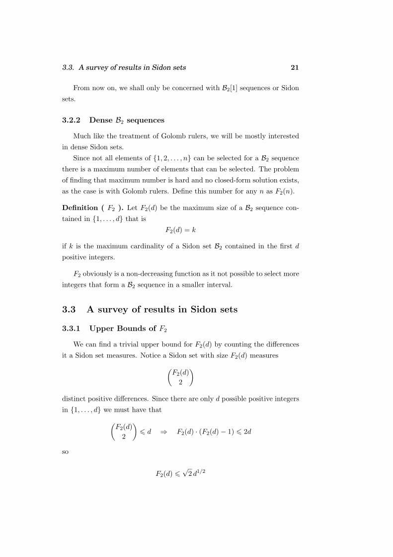
We can find a trivial upper bound for F2(d) by counting the differences
it a Sidon set measures. Notice a Sidon set with size F2(d) measures
(F2(d)
2
)
distinct positive differences. Since there are only d possible positive integers
in {1, . . . , d} we must have that
(F2(d)
2
)6 d ⇒ F2(d) · (F2(d)− 1) 6 2d
so
F2(d) 6√
2 d1/2

22 Chapter 3. Sidon Sets
Erdos and Turan were the first to improve this bound in 1941. They
proved in [25] that
F2(d) 6 d1/2 + O(d1/4)
This lower bound was further improved by Lindstrom[42] and indepen-
dently by Klazar[33] and the following is, as of today, the tightest upper
bound known. We will provide a simple combinatorial proof similar to the
one of Lindstrom.
Theorem 3.1 (Lindstrom).
F2(d) < d1/2 + d1/4 + 1
Proof. Let A = a1 < a2 < . . . < ar be a B2 sequence from the set
{1, 2, . . . , d}. The differences aj − ai , 1 6 i < j 6 r must be all differ-
ent. We call the positive number j − i the order of the difference aj − ai.
For a given order ν consider the sum of all differences of order ν
Σν =r−ν∑
i=1
(ai+ν − ai)
The sum can be split in ν sequences of the form
(aν+1 − a1) + (a2ν+1 − aν+1) + (a3ν+1 − a2ν+1) + . . .
(aν+2 − a2) + (a2ν+2 − aν+2) + (a3ν+2 − a2ν+2) + . . .
...
As a result of cancellations, each of the ν sequences has sum at most d
and the total sum of all differences of order ν is at most νd.
Consequently, the sum of all differences of order at most m is at most
Σ1 + Σ2 + . . . + Σm < (1 + 2 + . . . + m)d =12m(m + 1)n. (3.1)
There are r−ν differences of order ν. The number of differences of order
3.3. A survey of results in Sidon sets 23
at most m is
(r − 1) + (r − 2) + . . . + (r −m) = mr − 12m(m + 1) = ms
where s = r − 12(m + 1). Since all these differences must be different, we
find that
Σ1 + Σ2 + . . . + Σm > 1 + 2 + . . . + ms =12ms(ms + 1) (3.2)
Using equations 3.1 and 3.2 and the inequality ms(ms + 1) > m2s2, we
bound s from above
12m2s2 <
12m(m + 1)d =⇒ s < n1/2
√1 + m−1
To simplify the expression, notice that for all x,√
1 + x < 1+ 12x and let
x = m−1. Moreover, since m−1 is less than 1, we have a good approximation√1 + x ≈ 1 + 1
2x of the radical. By substituting s we get
r <12(m + 1) + d1/2(1 +
12m−1)
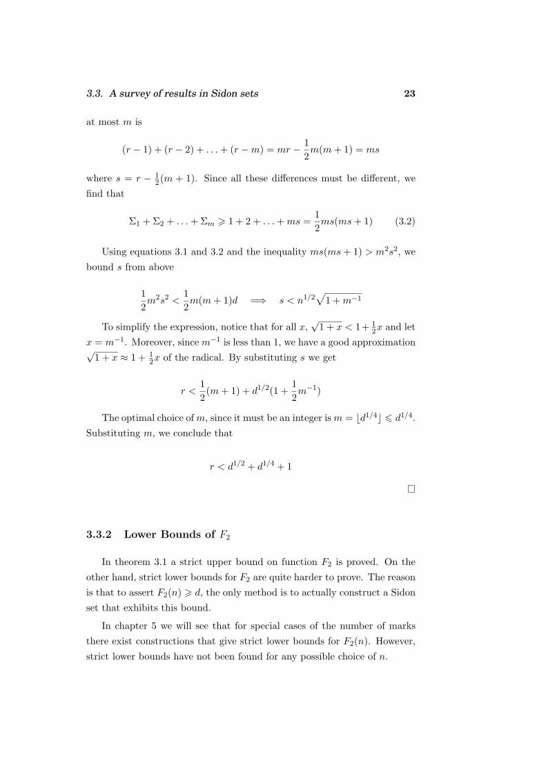
The optimal choice of m, since it must be an integer is m = bd1/4c 6 d1/4.
Substituting m, we conclude that
r < d1/2 + d1/4 + 1
3.3.2 Lower Bounds of F2
In theorem 3.1 a strict upper bound on function F2 is proved. On the
other hand, strict lower bounds for F2 are quite harder to prove. The reason
is that to assert F2(n) > d, the only method is to actually construct a Sidon
set that exhibits this bound.
In chapter 5 we will see that for special cases of the number of marks
there exist constructions that give strict lower bounds for F2(n). However,
strict lower bounds have not been found for any possible choice of n.

24 Chapter 3. Sidon Sets
The best lower bound known which is asymptotic to n2 is
F2(n) > n1/2 −O(n5/16)
which has been proved by Erdos and Turan [25].
3.3.3 Well Distribution in residue classes
Lindstrom [44] has proved that the numbers that form a Sidon sequence
of size more than n1/2 are well distributed in residue classes modulo m. That
is about 1/m of all the elements fall in each of the m residue classes.
Theorem 3.2 (Lindstrom). Let A ⊆ [1, n] be a Sidon set with r = |A| =(1 + o(1))n1/2. For a fixed integer m > 2 let Ai = {a ∈ A : a ≡ i (mod m)}and ri = |Ai|, 0 6 i < m. Then ri/
√n → 1/m when n →∞.
He also proved than in the special case when m = 2 the number of even
and odd elements is almost equal.
Theorem 3.3 (Lindstrom). Let A ⊆ [1, n] be a Sidon set of size r > n1/2.
Then for the number r0 of even elements and the number r1 of odd elements
|r0 − r1| < 4√
r3/20 + r
3/21 = O(n3/8).
Kolountzakis [39] has proved a more general result that does not impose
the restriction of Lindtrom’s theorem on the number of elements of the Sidon
set. Let
Theorem 3.4 (Kolountzakis). Let A ⊆ [1, n] be a Sidon set with size
r = |A| > n1/2 + l(n)
where l(n) = o(n1/2).
For each modulus m define
a(x) = |{a ∈ A : a ≡ x (mod m)}|
be the number of elements that fall in each residue class. Then, if m =
o(n1/2)
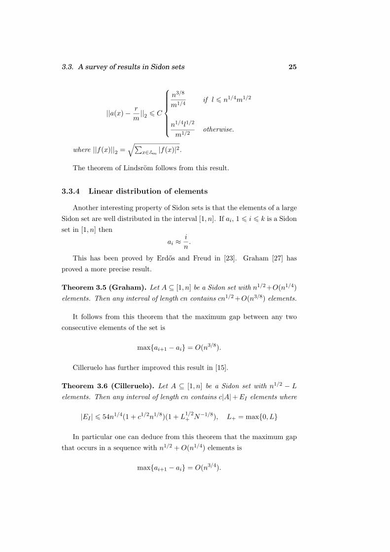
3.3. A survey of results in Sidon sets 25
||a(x)− r
m||2 6 C
n3/8
m1/4if l 6 n1/4m1/2
n1/4l1/2
m1/2otherwise.
where ||f(x)||2 =√∑
x∈Zm|f(x)|2.
The theorem of Lindsrom follows from this result.
3.3.4 Linear distribution of elements
Another interesting property of Sidon sets is that the elements of a large
Sidon set are well distributed in the interval [1, n]. If ai, 1 6 i 6 k is a Sidon
set in [1, n] then
ai ≈ i
n.
This has been proved by Erdos and Freud in [23]. Graham [27] has
proved a more precise result.
Theorem 3.5 (Graham). Let A ⊆ [1, n] be a Sidon set with n1/2+O(n1/4)
elements. Then any interval of length cn contains cn1/2 +O(n3/8) elements.
It follows from this theorem that the maximum gap between any two
consecutive elements of the set is
max{ai+1 − ai} = O(n3/8).
Cilleruelo has further improved this result in [15].
Theorem 3.6 (Cilleruelo). Let A ⊆ [1, n] be a Sidon set with n1/2 − L
elements. Then any interval of length cn contains c|A|+EI elements where
|EI | 6 54n1/4(1 + c1/2n1/8)(1 + L1/2+ N−1/8), L+ = max{0, L}
In particular one can deduce from this theorem that the maximum gap
that occurs in a sequence with n1/2 + O(n1/4) elements is
max{ai+1 − ai} = O(n3/4).

26 Chapter 3. Sidon Sets
3.4 Summary
In this chapter, Sidon sets were introduced and the known properties of
the elements of a Sidon set were reviewed.
The elements of Sidon sets have all the good properties one might hope:
they are well distributed linearly inside the selected interval, they are well
distributed in residue classes and their size is about n1/2. However all the
theorems that have been proved only provide asymptotic results.
When one looks into a Sidon set more closely the (small asymptotically)
variation between exact linear distribution and the actual distribution of the
elements is significant. Moreover, the difference between n1/2 and the size
of a Sidon set can approach to 0 as a limit but this difference is enough to
make the problem of determining the exact maximum size of a Sidon set
still an open problem.
Chapter 4
Equivalence of the two
problems
Sidon sequences and Golomb rulers have equivalent definitions, as we will
shortly prove. However, no systematic treatment of the relation between the
two problems has been done up to now. In fact, some authors seem to ignore
the relation between the two problems and reprove old results using their
own methods. Distinct notation is what has prevented bounds between the
two equivalent problems to be united.
We will study the equivalence between the two problems and unite in
some sense the results on bounds of the sizes of Sidon sets and Golomb
rulers. Theorems that will allow future results on one problem to be easily
restated to the other will be presented.
Using the main result of this chapter, theorem 4.5, we will prove an
improved lower bound in theorem 4.9 for the length of optimal Golomb
rulers.
4.1 Equivalence of Sidon sets and Golomb rulers
From a quick look at the definition of Sidon sets it is not hard to notice
the relation to the Golomb ruler problem: a set having distinct differences
between any two elements will also have distinct sums and vice versa. To
illustrate this, consider that for any four elements ai, aj , ak, al we have that
ai + aj = ak + al ⇐⇒ ai − ak = al − aj . (4.1)
27

28 Chapter 4. Equivalence of the two problems
Now we can prove that the two definitions are equivalent.
Proposition 4.1. If a set A is a B2 sequence then it is a Golomb ruler and
vice versa.
Proof. Suppose that A is B2 but not a Golomb ruler. Since it not a Golomb
ruler, there must exist elements ai, aj , ak, al with ai − aj = ak − al. This
would imply, by equation 4.1, that ai + al = ak + aj , a contradiction since
it is a Sidon set.
Now suppose A is a Golomb ruler but not a Sidon set. Since it is not a
B2 sequence, there must exist elements ai, aj , ak, al having ai + aj = ak + al
with {i, j} 6= {k, l}.At most 2 of these elements can be identical and suppose i 6= l. Then
we can arrange them in differences ai − al = ak − aj with {i, l} 6= {k, j}.This is a contradiction since the original set is a Golomb ruler.
If we view B2 sequences in Golomb ruler terms, F2(d) is the maximum
number of marks that can be placed in the interval {1, . . . , d}.
4.2 Relations between G(n) and F2(n)
In the past many authors have worked independently between the two
problems. Sometimes essentially the same results have been reproved and
published in different journals, like the fact that G(n) asymptotically ap-
proaches n2 as n → ∞. It has been proved by Singer and Erdos but has
been republished in [5] in 1986.
To enable us to restate results between the two problems, an investigation
of the relation between G(n) and F2(n) will be presented. Remember that,
by definition 2.1.2 (page 8), G(n) is the minimum length of a Golomb ruler
with n marks.
It is should be clear by now that between these two function there is
some sense of inverse relation: G(n) refers to the minimum size of a Golomb
ruler given the number of marks and F2(n) refers to the maximum number
of marks in relation to the length of the ruler.

4.2. Relations between G(n) and F2(n) 29
4.2.1 Equality relations
First, we will consider equality relation between the two functions. We
will prove two lemmas that will help us later prove our two main theorems
for inequality relations.
Notice that B2 sequences do not necessarily begin at 1 or end at n.
However since every B2 sequence is a Golomb ruler, the two properties of
translation and mirroring also apply. By the translation A′ = A−min{ai}we get a Golomb ruler that begins at position 0 from any B2 sequence.
First suppose that we know the exact value of F2(d) for some d. The
following lemma tells us what we can learn about G(n).
Lemma 4.1. For every d, if
F2(d) = n ⇐⇒ G(n) 6 d− 1
G(n + 1) > d− 1
Proof. If the maximum size of a Sidon set contained in {1, . . . , d} is n then
there is a Golomb ruler with k marks that has elements
A′ = {ai −min(ai) ∀ai ∈ A}
where A is the Sidon set and min(ai) it’s minimum element which is at least
1. This ruler begins at position 0 and has length 6 d− 1 thus G(n) 6 d− 1.
Also, since at most n marks can be placed in {1, . . . , d}, also at most n
marks can be placed in {0, . . . , d− 1}. It follows that G(k + 1) > d− 1.
For the opposite direction notice that if the two inequality relations
hold for G(n) then at most n marks can be placed in {0, . . . , d − 1} (and
G(n) 6 d − 1 guarantees that such placement exists) or equivalently in
{1, . . . , d}, so F2(d) = n.
Inversly, if we know for some n an exact value of G(n), the following
lemma will help us find two exact values for F2(d).
Lemma 4.2. For every n, d, if
G(n) = d ⇐⇒ F2(d) = n− 1
F2(d + 1) = n

30 Chapter 4. Equivalence of the two problems
Proof. If G(n) = d then there exist a Golomb ruler contained in the set
{0, 1, . . . , d} with n marks but no such ruler exists in {0, 1, . . . , d− 1}.In turn, by the translation property a Sidon set with n elements exists
contained in {1, 2, . . . , d+1} which means that F2(d+1) > n. But F2(d+1)
cannot be n + 1 as it would imply that G(n + 1) = d and G is strictly
increasing so F2(d + 1) = n.
Also, since G(n) = d and G is monotonically increasing (lemma 2.2), we
have that G(n − 1) 6 d − 1 and G(n) > d − 1. These two inequalities and
lemma 4.1 imply that F2(d) = n− 1.
For the opposite direction, F2(d + 1) = n implies that n marks can be
placed in [1, d+1] or equivalently in [0, d]. By F2(d) = n−1, n marks cannot
be placed in [0, d− 1] and consequently G(n) = d.
It is evident that the two functions can provide us with the same in-
formation of the properties of the Sidon sets and Golomb rulers. In some
sense, exact values of G are stronger than exact values of F2, since the for-
mer transform directly into two exact values of F2 while the opposite does
not hold. However, complete knowledge of the values of one function, either
G or F2, provides the values of the other function.
4.2.2 Inequality relations
Less that 25 exact values are known for G or F2. Most results concerning
these two functions are in the form of lower and upper bounds for the exact
value. To be able to translate these results between the two problems we
must translate inequality relations between F2 and G.
First consider the case that we know a lower or an upper bound for
F2(d). The following two lemmas will help in bound G(n).
Lemma 4.3. For every n, d if
F2(d) > n =⇒ G(n) < d− 1
Proof. Suppose F2(d) = n′ > n. Then by lemma 4.1: G(n′) 6 d− 1. Since
n′ > n and G(n) is monotonically increasing by lemma 2.2, we have that
G(n′) > G(n) so
G(n) < G(n′) 6 d− 1
4.2. Relations between G(n) and F2(n) 31
Lemma 4.4. For every n, d if
F2(d) < n =⇒ G(n) > d− 1
Proof. Suppose F2(d) = n′ < n. Then by lemma 4.1: G(n′ + 1) > d − 1.
Since n > n′ + 1 ⇒ G(n) > G(n′ + 1) so
G(n) > G(n′ + 1) > d− 1
These two lemmas enable us to bound G using known bounds for F2.
Suppose that we have a function l(d) that bounds F2 from below: F2(d) >
l(d) for each d. Usually l(d) will be a monotonically increasing function so
it admits an inverse function l−1(n), so that l−1(l(d)) = d. Then if for all d:
F2(d) > l(d) =⇒ G(l(d)) < d− 1 =⇒
G(n) < l−1(n)− 1 (4.2)
Accordingly, if F2(d) < u(d) for each d and u−1(n) exists then G(n) >
u−1(n)− 1
We have proved that
Theorem 4.5. Suppose l(d) and u(d) are well-defined and admit inverse
functions l−1(n) and u−1(n) inside an interval A ⊆ N. If
l(d) < F2(d) < u(d)
then
u−1(n) < G(n) + 1 < l−1(n)
Now consider the opposite case where we know some bound for G(n)
and wish to bound F (d).
Lemma 4.6. For every n, d if G(n) < d then F2(d) > n
Proof. Since G(n) < d, there exists a Golomb ruler with n marks having
0 = a1 < a2 < . . . < an < d.

32 Chapter 4. Equivalence of the two problems
The B2 sequence bi = ai + 1 is contained in [1, d] since bn 6 d so F2(d)
is at least n.
Lemma 4.7. For every n, d if G(n) > d then F2(d) 6 n.
Proof. By the hypothesis, in the set {0, . . . , d} we cannot select n marks.
That implies that the maximum number of integers we can select from
{1, . . . , d + 1} is less that n. Then, F2(d + 1) < n and also F2(d) 6 n
since F2 is non-decreasing.
The following theorem unites the two lemmas
Theorem 4.8. Suppose l(n) and u(n) are well-defined and admit inverse
functions l−1(d) and u−1(d) inside an interval A ⊆ N. If
l(n) < G(n) < u(n) then u−1(d) 6 F2(d) 6 l−1(d)
4.3 Improving lower bounds of G(n)
By using the upper bound we proved for F2 we can find a better lower
bound for the optimal length of Golomb rulers.
Theorem 4.9. For all n
G(n) > n2 − 2n√
n +√
n− 2
Proof. By theorem 3.1 we know that F2(d) < d1/2 + d1/4 + 1. Consider the
function u(d) = d1/2 +d1/4 +1. This function is monotonically increasing in
the interval (0,∞) and we can find it’s inverse by the substitution d = y4.
Solving for y we have that
y =√
n− 3/4− 1/2
and consequently
u−1(n) =(√
n− 34 − 1
2
)4
(4.3)
= n2 − 2n√
n− 34 +
√n− 3
4 − 12 (4.4)
(4.5)

4.3. Improving lower bounds of G(n) 33
Using theorem 4.5 we find that
G(n) > n2 − 2n√
n− 34 +
√n− 3
4 − 32 (4.6)
> n2 − 2n√
n +√
n− 34 − 3
2 (4.7)
By the inequality√
n− 34 > √
n− 12 for n > 1 , we conclude that
G(n) > n2 − 2n√
n +√
n− 2
This is an improvement over the trivial lower bound G(n) > 12n(n − 1)
for n > 13. As n becomes larger the gap between the two bounds increases.
In figure 4.3 the bound we proved is compared against the trivial lower
bound 12n(n − 1) and the known optimal values of the length of Golomb
rulers for n < 24.
0 5 10 15 20number of marks
0
100
200
300
400
500
leng
th
best known lengthlower boundn*(n-1)/2
Figure 4.1: Lower bounds known versus known optimal ruler sizes

34 Chapter 4. Equivalence of the two problems
4.4 Summary
Golomb rulers and Sidon sets are closely related: both have equivalent
definitions. In this chapter we discussed the relation between F2(n) and
G(n), the two functions that give the best possible size of a Sidon set or
length of a Golomb ruler and proved theorems that allow the restatement of
known or future results on G(n) or F2(n) to the other problem. Using these
results we have derived a better lower bound for G(n) which is contained in
theorem 4.3.

Chapter 5
Constructions for Golomb
rulers
When the number of marks exceeds 25, brute-force algorithms that
search all the possible rulers do not stand a chance of finding a near-optimal
ruler with size less that n2. In this case one has to resort to algebraic con-
structions that generate sequences of integers having a priori the desired
properties.
In this chapter we will consider constructions that generate Golomb
rulers with large number of marks and size near n2. All of our construction
will be based on the properties of finite fields.
We will first introduce basic facts from number theory and finite fields
for the reader which is not acquainted with the subject and then we will
describe the constructions.
The main constructions we will use are the Bose-Chowla construction de-
scribed in [11] and I. Ruzsa [50] construction as extended by Lindstrom[43].
5.1 Introduction to number theory
Before we begin describing the constructions for Golomb rulers (and
Sidon sets) we will first give a quick review of the number theoretic facts we
will use from now on. For a more complete treatment see the classic text in
number theory by Hardy and Wright[30].
The reader who is acquainted with number theory and finite fields can
skip this section.
35

36 Chapter 5. Constructions for Golomb rulers
5.1.1 Prime numbers and Euler’s φ fucntion
An integer a > 1 is prime if it has no other divisors but 1 and a. Primes
have many special properties and play a critical role in number theory. The
first few primes are:
2, 3, 5, 7, 11, 13, 17, 19, 23, 29, 31, 37, 41, 43, 47
If a number is not prime it is a composite number. For example 39 is
composite as 39 = 3 ∗ 13. The integer 1 is neither a prime nor a composite
and is called a unit. Similarly 0 is neither prime or composite.
For every two integers a, b we can find the largest integer that divides
both of then. This integer is called the greatest common divisor of a
and b and is symbolized as gcd(a, b) or more commonly just (a, b).
If a, b do not share common divisors larger that 1 then they are relative
prime and (a, b) = 1. For example, 8 and 15 are relative prime since no
integer larger than 1 divides both of them.
For a given number n, the number of integers, smaller than a, that are
relative prime to n is symbolized as φ(n), the Euler’s phi function. By
|S| we denote the number of elements of set S.
φ(n) = |{a < n and gcd(a, n) = 1}|
For example φ(10) = 7 since the integers that do not share a common divisor
with 10 are 7 : 1, 3, 4, 6, 7, 8, 9.
Note that if p is a prime number then neither of the integers 1, 2, . . . , p−1
has a common divisor with p so
φ(p) = p− 1 if p is prime
5.1.2 Integer division
Elementary mathematics state that every integer a when divided by b
has an unique integer quotient q and remainder r, so that a = q · b + r. For
example 26 divided by 3, gives q = 8 and r = 2: 26 = 8 · 3 + 2.
Theorem 5.1 (Division). For every integer a and b, there are unique
5.1. Introduction to number theory 37
integers q and r so that 0 6 r < b and
a = q · b + r.
Proof. Suppose that there exist two different solutions
a = q1b + r1 = q2b + r2.
q1 must be different from q2, so (q1 − q2)b = r1 − r2 must be a non-zero
multiple of b. Consequently it is greater than b in absolute value.
We must have that |r2 − r1| > b, a contradiction since −b < r2 − r1 < b
by 0 6 r1, r2 < b.
The integer q is called the modulus of a when divided by b and as we
shown it belongs to the interval [0, b− 1]. Usually we denote it as
a mod b = q or (a)b = q
If q = 0 then b divides a and we write b|a. Of course if b|a then a mod b = 0.
When two integers a1,a2 share the same modulus when divided by b we
say that they are equivalent modulo b and denote it as
a1 ≡ a2 mod b
For example 45 ≡ 25 mod 20.
The modulus has some important properties that will be very useful from
now on:
(a)n + (b)n ≡ a + b mod n (5.1)
(a)n · (b)n ≡ a · b mod n (5.2)
We can define addition and multiplication modulo some integer n as
normal addition and multiplication but taking the modulo n of the results.
Sometimes the symbols +n and ·n will be used to denote such operations.
Subtraction −n can be defined likewise. For example 2 +9 17 = 1 and
2 ·5 10 = 0.
These two operations and especially multiplication modulo p will play a
central role from now on so one must have a good grasp of the theory. We
will now define more formally these operations.

38 Chapter 5. Constructions for Golomb rulers
Define the set Zn = {0, 1, . . . , n − 1}. We can think Zn as the set of
all possible remainders modulo n. Suppose we have a, b ∈ Zn. Then also
a +n b is in Zn and always using +n we will never get outside of the set
Zn. Forgetting the usual addition, if we always use addition modulo n then
say that we belong to a group, more specifically the group of Zn under the
operation of addition modulo n. It is symbolized as group Z+n = (Zn, +n),
the additive group modulo n.
More generally a group is a set S together with an operation ¯ defined
on S and is symbolized as (S,¯). The following properties must hold for a
group:
1. Closure: For all a, b ∈ S, we have a¯ b ∈ S.
2. Identity: There exist an element e ∈ S, called the identity of the
group, such that e¯ a = a¯ e = a for all a ∈ S.
3. Associativity: For all a, b, c ∈ S, we have (a¯ b)¯ c = a¯ (b¯ c).
4. Inverse element: For each a ∈ S, there exists a unique element
b ∈ S, called the inverse of a, such that a¯ b = b¯ a = e.
The size of a group is the number of elements in it’s defining set. In this
case the number of elements in (Zn, +n) is |Zn| = n.
5.1.3 The multiplicative group modulo n
Another group, more interesting for our discussion, is the multiplica-
tive group modulo n, (Z∗n, ·n), where the operation is multiplication mod-
ulo n. It can be proved that 0 cannot be an element of the group and neither
can be any integer that has a common divisor with n or else there would
not be a unique inverse for each element .
So, only integers that are relative prime to n can be in this group. For
example Z∗15 = {1, 2, 4, 7, 8, 11, 13, 14}. By the definition of the Euler’s phi
function, the size of the group is |Z∗n| = φ(n).
We will only consider multiplicative groups with n being a prime number.
If p is prime then Z∗p = {1, 2, . . . , p− 1} and |Z∗p | = p− 1.
As multiplication is defined, we can also define powers of an element a
of Z∗p as

5.1. Introduction to number theory 39
Table 5.1: Powers of 2 and 3 in Z∗13
n 0 1 2 3 4 5 6 7 8 9 10 11 122n 1 2 4 8 3 6 12 11 9 5 10 7 13n 1 3 9 1 3 9 1 3 9 1 3 9 1
ak = a ·p a ·p a . . . a︸ ︷︷ ︸k times
Define also a0 = 1. The usual law of exponents holds: ak al = ak+l.
Since there are only φ(n) different elements in the multiplicative group,
the powers of a must repeat inevitably. Fermat’s theorem and Euler’s gen-
eralization state this fact.
Theorem 5.2 (Euler). For every element a of Z∗n,
aφ(n) ≡ 1 (mod n).
Corollary 5.3 (Fermat). If p is prime, then
ap−1 ≡ 1 (mod p).
So, if p is prime then ap−1+k = ap−1ak = ak that is, the powers of a
repeat after, at most, p− 1 steps. In the following table we list the powers
of 2 and 3 (mod 13) .
Notice that the powers of 3 repeat after 3 steps but the powers of 2
generate all the integers 1, 2, . . . , 12 in a permutation. The order ordpa of
an element is the period of it’s powers in Z∗p . In this case ord133 = 3 and
ord132 = 12.
Definition (order). The order of an element g of Z∗p is the least positive
integer z for which gz ≡ 1 (mod p). We will use the notation ordpg to refer
to the order of element g in Z∗p .
We can classify the elements of Z∗p in two categories: If the powers of a
cycle through all elements of group Z∗p or equivalently if ordpa = p− 1 then
a is called a primitive element of Z∗p . On the other hand, if ordpa < p− 1
then a is a not primitive.

40 Chapter 5. Constructions for Golomb rulers
Definition (primitive element). If gi ≡ 1 (mod p) does not hold for
1 6 i 6 p − 1, or equivalently ordpg = p − 1, then g is called a primitive
element of Z∗p .
Primitive elements are also called generators of Z∗p since the powers of
g generate all the elements of the field. For a primitive element the powers
g0, g1, . . . , gp−1 are a permutation of 1, 2, . . . , p− 1.
An important property of primitive elements is that
gi = gj ⇐⇒ i = j (5.3)
for i, j < p− 1, since the elements gi are unique.
In our example 2 is a primitive element as the values of 2n for 1 6 n 6 12
are exactly the integers 1, 2, . . . 12. On the other hand the powers of 3 repeat
with period 3 and it is not a primitive element.
To find primitive elements the following will be useful.
Lemma 5.4. The order of an element g of Z∗p divides p− 1.
Proof. We know, by Fermat’s theorem 5.3, that gp−1 ≡ 1 (mod p). Let t be
the order of g so gt ≡ 1 (mod p).
Suppose t does not divide p− 1, then by the division theorem
p− 1 = u · t + v
with v 6= 0 and v < t. Now we have that:
gp−1 ≡ gutgv ≡ (gt)ugv ≡ 1ugv ≡ gv
Since gp−1 ≡ 1 (mod p) then we have that gv ≡ 1 (mod p). This is a
contradiction because v < t and we assumed t is the least positive integer
for which gt ≡ 1 (mod p).
Corollary 5.5. If gi ≡ 1 (mod p) does not hold for 1 6 i 6 bp−12 c then g
is a primitive element of Z∗p .
Proof. By 5.4, if gi 6= 1 (mod p) for i 6 bp−12 c then the order of g is greater
than 12(p− 1). Since there are no numbers greater than 1
2(p− 1) that divide
p− 1 before p− 1 itself, the period of g is p− 1.

5.2. A simple construction 41
Later, we will be interested in findind all the primitive roots of Z∗p .
Instead of trying every element of Z∗p to see if it’s order is p− 1, we can use
the following lemma to find all the primitive elements after we have found
the first. The proof is omitted.
Lemma 5.6. If g is a primitive root of Z∗p then gn is also a primitive root
if and only if gcd(n, p− 1) = 1.
By using this lemma, we can find the exact number of primitive roots in
Z∗p which is the number of integers n such that gcd(n, p− 1) = 1.
Lemma 5.7. There are exactly φ(p− 1) primitive roots in the group Z∗p .
5.1.4 Finite fields
We have described the multiplicative group Z∗n for any n. When n is a
prime number p then the elements of the group are all the positive integers
1,2,. . .,p− 1 since none of them has a common divisor with p.
Groups with prime number of elements have some additional properties
and they have a special name, finite fields. The theory of finite fields began
with the work of Carl Friedrich Gauss (1777-1855) and Evariste Galois (1811-
1832) but it only became of interest for applied mathematicians in recent
decades with the emergence of discrete mathematics and the applications
in cryptography and other areas. In honor of Galois the finit field with p
elements is denoted as GF (p).
It can be proved that finite fields exist not only for prime numbers,
but also for any power of a prime number pn. The field GF (pn) is called
an extension field of GF (p). When n > 1, extension fields are difficult
to describe and we will not continue the discussion here. For a complete
treatment of finite fields see [41] or any modern algebra book.
5.2 A simple construction
Before we describe more subtle constructions, we will first see a simple
one which follows from elementary mathematics.
Construction 1. Let n be any positive integer. Then the sequence
Φ0(a) = 2na2 + a , 0 6 a < n
42 Chapter 5. Constructions for Golomb rulers
forms a Golomb ruler.
Proof. Suppose we have the sum of two elements
Φ0(a) + Φ0(b) = 2n(a2 + b2) + (a + b) (5.4)
Consider the division of Φ0(a) + Φ0(b) by 2n. By the division algorithm
there exist unique integers q, r with 0 6 r < 2n such that
Φ0(a) + Φ0(b) = 2n q + r (5.5)
But since 0 6 a + b < 2n, by equation 5.4 we have q = a2 + b2, r = a + b.
This system has a unique solution (up to permutation) for a, b,
{a, b} =12(r ±
√2q − r2)
and so there cannot be two different pairs of elements which have the
same sum.
With a more complex argument, using the differences instead of the
sums, it can be shown that dropping the 2 from equation 5.4 will also result
in a Golomb ruler.
Construction 2. Let n be any positive integer. Then the sequence
Φ1(a) = na2 + a , 0 6 a < n
forms a Golomb ruler.
The largest element of this sequence is n3− 2n2 + 2n which implies that
for all n an upper bound for the optimal length of a Golomb ruler is
G(n) 6 n3 − 2n2 + 2n.
Computing these two construction is straightforward and takes time
O(n) for every n. In fact the computations can be arranged so that Θ(n)
additions and multiplications are necessary.

5.3. Erdos and Turan construction 43
5.3 Erdos and Turan construction
Erdos and Turan [25], have given the first construction which lowers the
bound and provides rulers with size Θ(n2).
Unfortunately this construction and all constructions which produce
rulers of size Θ(n2) do not work for all choices of prime numbers but only
for primes (or prime powers).
Construction 3. For every prime number p the following sequence forms
a Golomb ruler
2p a + (a2)p , 0 6 a < p
This construction was used by Erdos to prove the first upper bound on
Sidon sets and consequently Golomb rulers. For for p prime, it is implied
by the construction that
G(p) 6 2p2 − p− 1
.
Again, it is easy to compute the elements of this construction in time
O(p) using Θ(p) multiplications and additions.
Unfortunately this construction does not produce Golomb rulers of size
less than n2, so we will not be able to use it for out purposes.
5.4 Ruzsa construction
The first construction we will discuss that gives rules of size near n2 was
given by I.Z. Ruzsa in [50].
It is a very fast construction which gives Golomb rulers with p − 1 ele-
ments for every prime number p and size p2 − p.
The computations used are straightforward and can be developed to a
very efficient algorithm that is able to find sequences with more than 10000
marks.
We will use some more complicated arguments in this proof regarding
finite fields. For the related theorems, see any basic treatment of finite fields
like [41].

44 Chapter 5. Constructions for Golomb rulers
Construction 4 (Ruzsa). Let p be a prime number and g a primitive
element of the multiplicative group Z∗p . The following sequence is a Golomb
ruler.
R(p, g) = pi + (p− 1)gi mod p(p− 1) for 1 6 i 6 p− 1
Proof. Let
p(i + j) + (p− 1)(gi + gj) ≡ a (mod p)(p− 1)
be the sum of two elements. Then we can find that
gi + gj ≡ −a (mod p) (5.6)
i + j ≡ a (mod p− 1) (5.7)
By Fermat’s little theorem 5.3 that we proved earlier in page 39:
gigj ≡ ga (mod p) (5.8)
By 5.6 and 5.8, gi and gj are the roots of the quadratic polynomial
X2 + aX + ga in GF (p), so
X2 + aX + ga = (X − gi)(X − gj).
From the uniqueness of the factorization of a quadratic polynomial in GF (p)
we infer the uniqueness of gi, gj and consequently of i,j up to a permutation.
For an example when p = 7, the primitive elements elements of Z∗7 are
3 and 5. Then
R(7, 3) = {6, 10, 15, 23, 25, 26}
R(7, 5) = {6, 11, 15, 37, 38, 40}
Lindstrom [43] has proved that if f is an integer relative prime to p− 1
then the following is also a Golomb ruler:
R′(p, g, f) = pfi + (p− 1)gi mod p(p− 1) for 1 6 i 6 p− 1
He has also proved in the same paper that by varying the primitive

5.5. Singer Perfect Difference sets 45
element and f , one does not produce new Golomb ruler but a translation
of the original one multiplied by an integer modulo p(p − 1). Since the
extended construction is equivalent to the original one, we will not consider
this extension.
The p−1 integers in R(p, f) are reduced modulo p(p−1) and the largest
of them is smaller than p(p− 1). The following bound for G(n) follows
Lemma 5.8. G(n) < n2 + n whenever n+1 is prime
The computation of R(p, g) depends on finding a primitive element of the
appropriate finite field. The construction assumes that a primitive element
of the associate finite field can be found fast. We will see in the next chapter
that this actually holds and the time of computing all the primitive elements
of Z∗p can be found in time neglible to the other operations.
Assuming that a primitive element is found, the algorithm will take time
O(p) to find all the elements of a Golomb ruler. However the elements will
not be necessary in increasing order so a sorting algorithm has to be used.
Linear time sorting algorithms exists [4], so the total time to produce a
Golomb ruler in sorted order can be O(p). However the constants involved in
linear time sorting algorithms are large and classical sorting approaches are
more efficient. We will use a classical comparison based sort like mergesort
[16] to provide an upper bound of O(p log p) for the total running time.
5.5 Singer Perfect Difference sets
Singer [53] has proved that if q is a power of a prime then we can find
q + 1 integers which have distinct differences modulo q2 + q + 1 and thus
form a Golomb ruler. Singer’s construction depends on the evaluation of
extensions of Galois fields, actually GF (p3) the 3rd order extension of the
multiplicative field Z∗p .
We will omit the proofs of this construction (as well as the next one);
they are quite complicated and beyond the scope of this discussion.
The reader who wishes to find more can refer to [41] or any modern
algebra book for a general discussion of the properties of finite fields of
higher order. The original proof is in [53].

46 Chapter 5. Constructions for Golomb rulers
Construction 5 (Singer). Let q = pn be a prime power. There there exist
q + 1 integers
d0, d1, . . . , dq
such that the q2 +q differences di−dj(i 6= j) when reduced modulo q2 +q+1,
are all the different non-zero integers less than q2 + q + 1.
This implies that whenever n − 1 is a prime power then, by the substi-
tution q + 1 = n, G(n) < n2.
Corollary 5.9. G(n) < n2 − n + 1 whenever n− 1 is a prime power.
The time required to compute Singer’s construction is of the order O(p3),
quite prohibitive for use in our computations.
5.6 Bose-Chowla theorem
Bose [11] and Chowla [12] have proved that for any prime power pn there
exist pn integers which form a Golomb ruler modulo p2n − 1.
Construction 6 (Bose). Let q = pn be a power of a prime and θ a primitive
element in the Galois field GF (q2). Then the q integers
d1, . . . , dq = {a : 1 6 a < q2 and θa − θ ∈ GF (q)} (5.9)
have distinct pairwise differences modulo q2 − 1.
In addition the q(q − 1) differences di − dj, i 6= j, when reduced modulo
q2 − 1, are all the different non-zero integers less than q2 − 1 which are not
divisible by q + 1.
For example when q = 11, θ = 2x+3 is a primitive element of GF (112).
The following sequence which is generated by equation 5.9
1, 6, 20, 27, 38, 40, 55, 65, 71, 117, 118
has distinct sums and differences modulo 120.
The largest element of this sequence is smaller than q2 − 1, so Bose-
Chowla theorem implies that whenever q = pn, a Golomb ruler with size
less that the square of the number of marks exists.

5.7. Shifting and multiplying a construction 47
Corollary 5.10. G(q) < q2 − 1 whenever q is a prime power.
We will use the construction of Bose later for the case of prime numbers
(n = 1) to find near-optimal Golomb rulers. Assuming that one can find a
primitive element of the field GF (q2) fast usually by a randomized algorithm,
computing the sequence takes time O(q2).
5.7 Shifting and multiplying a construction
The three constructions we described that produce rulers of size near n2,
work only for a prime (or power of a prime) number of marks. From these
constructions we will be using two transformations similar to the ones of
Golomb rulers we discussed in chapter 2: addition and multiplication.
Using these two properties one can find new Golomb rulers from the
given ones which also have about the same size. Then one can remove some
elements of the sequence to get rulers with a smaller number of marks for the
purpose of covering the gaps between prime numbers where no construction
for Golomb ruler exists. We will be using this properties to prove that
G(n) < n2 for all n smaller than a limit and not just prime numbers.
Note that having different pairwise sums modulo some integer z is some-
what stronger than just having different pairwise sums. This is the case as
between two elements ai > aj there exist two distances. The first is the
positive difference ai − aj like the case of Golomb rulers. The other one is
aj − ai which is also positive mod z and must be different from all other
distances.
To illustrate this, modular constructions can be thought as points on
the circumference of a circle. See for example figure 5.7 where a sequence
constructed by Bose-Chowla theorem {1, 2, 5, 11, 31, 36, 38} mod 48 is visu-
alized in the circumference of the circle and then unwound to form a Golomb
ruler of length 38.
The arc distance between any two points in a modular construction
must be different. There are n(n− 1) different arc lengths because between
each two elements there are two distances, one clockwise and one counter-
clockwise. So compared to 12n(n− 1) different distances for a Golomb ruler,
it is twice as hard to find a modular construction.
In a modular construction the important property is the modulus z. The
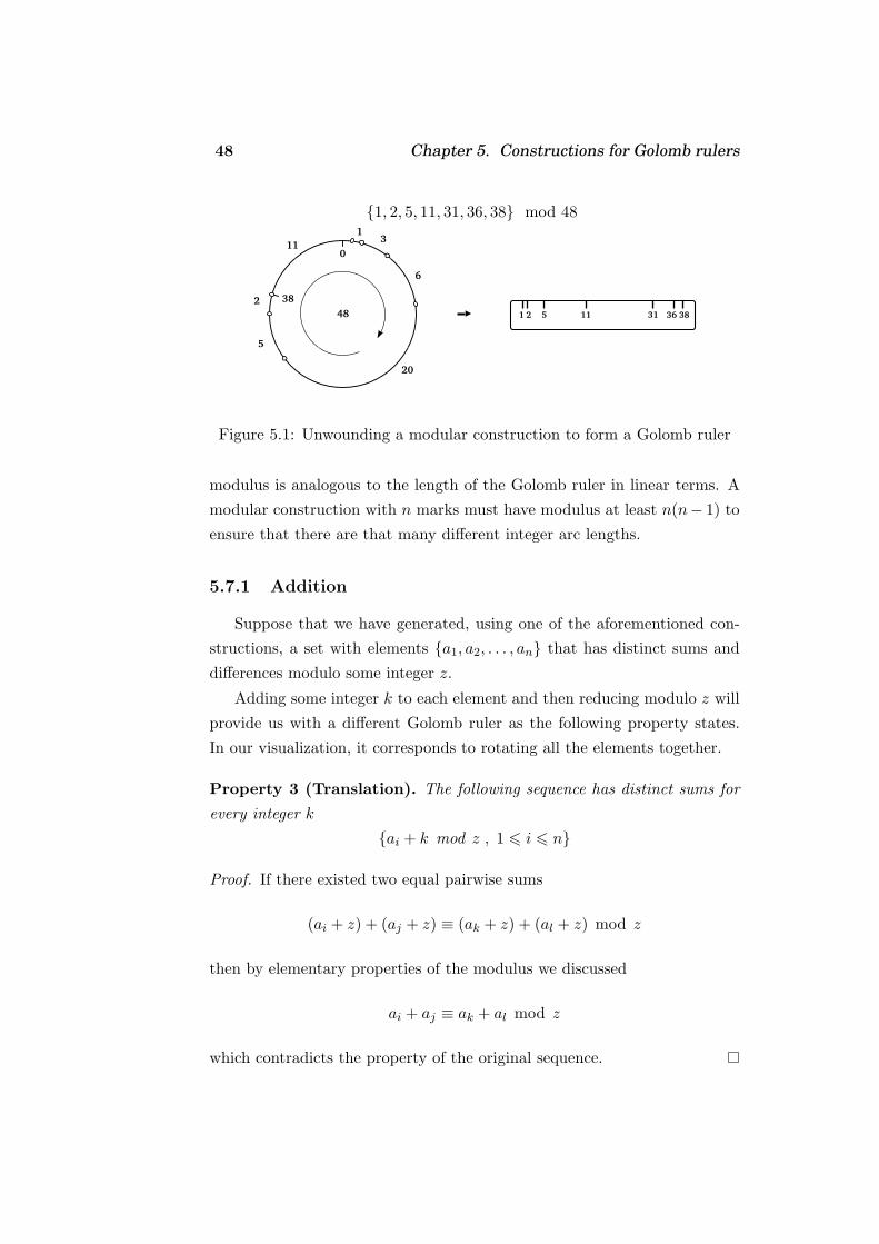
48 Chapter 5. Constructions for Golomb rulers
{1, 2, 5, 11, 31, 36, 38} mod 48
Figure 5.1: Unwounding a modular construction to form a Golomb ruler
modulus is analogous to the length of the Golomb ruler in linear terms. A
modular construction with n marks must have modulus at least n(n− 1) to
ensure that there are that many different integer arc lengths.
5.7.1 Addition
Suppose that we have generated, using one of the aforementioned con-
structions, a set with elements {a1, a2, . . . , an} that has distinct sums and
differences modulo some integer z.
Adding some integer k to each element and then reducing modulo z will
provide us with a different Golomb ruler as the following property states.
In our visualization, it corresponds to rotating all the elements together.
Property 3 (Translation). The following sequence has distinct sums for
every integer k
{ai + k mod z , 1 6 i 6 n}
Proof. If there existed two equal pairwise sums
(ai + z) + (aj + z) ≡ (ak + z) + (al + z) mod z
then by elementary properties of the modulus we discussed
ai + aj ≡ ak + al mod z
which contradicts the property of the original sequence.

5.7. Shifting and multiplying a construction 49
By varying the element k, from 0 up to z − 1 we can get z different
Golomb rulers. Using other values of k would not give us any different
rulers since adding k to each element is equivalent to adding k mod z.
The importance of these new rulers is that in general the maximum
element of this ruler will be different when varying k:
maxi{ai} 6= max
i{ai + k}
In general to obtain the best ruler, one has vary k and find the minimum
of all the maximum elements obtained by different choices of k:
mink
maxi{ai + k}
We can find which value of k will lead to the shortest Golomb ruler. If
the smallest mark of the ruler after a translation a1 is greater 0 one could
shift the ruler left by a1 to find a shorter one. That means only the cases
of k when the smallest element is 0 are meaningful. In this case the largest
element is is z−di where di = (ai+1−ai)z is the set of the distances between
consecutive elements. The minimum for the largest element occurs when di
is maximum that is
mink
maxi{ai + k} = z −max{ai+1 − ai (mod z)}
where we assume that the each subscript ax is reduced modulo z: ai+z = ai.
Generalizing, when one has to remove k elements from the construction
to form a Golomb ruler, the maximum difference ai+1+k−ai must be found.
We will use the following lemma to find the minimal maximum element of
the sequence in this case.
Lemma 5.11. If, for a construction with n elements mod z, we have to
remove k > 0 elements then the minimal length of the sequence that can be
produced by the translation property is
z − max16i6n
{a(i+1+k)n− ai (mod z)}
Intuitevely, the way to obtain the shortest possible Golomb ruler is to
shift the maximum of the differences between consecutive elements ai+1−ai
and shift this difference so that it is placed after the largest mark of the

50 Chapter 5. Constructions for Golomb rulers
{1, 2, 5, 11, 31, 36, 38} mod 48
Figure 5.2: Forming a shorter ruler by shifting and truncating
ruler and the end of the modulus.
5.7.2 Multiplication
Consider again a construction {a1, a2, . . . , an} that has distinct sums and
differences modulo some integer z. The second important transformation
that allows to generate new Golomb rulers modulo z from a given one is the
multiplication with an element relative prime to z.
Property 4 (Multiplication). The following sequence has distinct sums
for ever integer c with gcd(c, z) = 1
{c · ai mod z , 1 6 i 6 n}Proof. If there existed two equal pairwise sums
(cai) + (caj) ≡ (cak) + (cal) mod z
then by elementary properties of the modulus we discussed we can drop c
from both sides of the equation, so
ai + aj ≡ ak + al mod z
which contradicts the property of the original sequence.

5.8. Summary 51
If gcd(c, z) 6= 1 then we cannot drop c and the generated sequence will
not be a Golomb ruler.
Again, by varying element c one can produce new Golomb rulers. There
is no general way to know before multiplying which value will give the short-
est Golomb ruler and one has to cycle through all values of c. Altogether
there are φ(z) values of c to consider by the definition of Euler’s function.
5.8 Summary
In this chapter we discussed various known constructions for Golomb
rulers and Sidon sets. These constructions yield near-optimal sets, although
many of the sets generated by these constructions were proved to be optimal.
The important property that the three most important constructions
(Singer, Bose-Chowla and Ruzsa) have is that they are modular: the sums
or differences between pairs of elements are distinct modulo some integer z.
This property allows us to use two similarity transformations to generate
new Golomb rulers from a given one. Using these two transformations one
can often improve the length of a given Golomb ruler produced from a
modular construction.
A downside is that the constructions that yield near-optimal rulers apply
only to prime or prime power number of marks. However by omitting some
elements of a set one can fill the gap between the prime numbers and yield
near-optimal Golomb rulers for any number of marks.

52 Chapter 5. Constructions for Golomb rulers

Chapter 6
Algorithms for near optimal
Golomb rulers
Today near-optimal Golomb rulers of sizes less than n2 for n smaller
than 150 are known. Most of these rulers have been found using the con-
structions we described in chapter 5 and suitable transformations using the
two properties discussed.
In this chapter we will be interested in finding quick algorithms that
can continue this search and find near-optimal Golomb rulers with sizes less
than n2 for a number of marks up to 65000.
Our aim is to prove that Golomb rulers with size less than n2 exist for
every number of marks up to 65000. To prove this statement rulers of such
size must be exhibited for all n. For this purpose, use of constructions
described in chapter 5 is needed.
The following theorem will be the mail goal of this and the following
chapter. The proof will be computational.
Theorem 6.1 (Main Theorem). Golomb rulers of size less than n2 exists
for all n < 65000. Equivalently
G(n) < n2 for n < 65000
or in Sidon set terms
F2(d) > n1/2 for all d < 4.2 · 109
53

54 Chapter 6. Algorithms for near optimal Golomb rulers
6.1 Old results
A number of conjectures on the growth of the functions F2 and G exist.
Originally, most of the conjectures were introduced for the Sidon problem.
An old conjecture by Erdos states that G(n) < n2, that is Golomb rulers
with sizes less that n2 exist for all n.
This has not been proven up to now despite efforts by many mathemati-
cians. The closest form that has been proven is that G(n) asymptotically
approaches n2 as n tends to infinity. It has been shown by Chowla[14] and
Erdos[25, Addendum] that
F2(n) > n1/2 − o(n1/2)
which implies by the results of chapter 4 that
G(n) 6 n2 + o(n2).
Computationally it has been proven that G(n) < n2 for all n < 150
using Golomb rulers constructed by Singer and Bose constructions. The
computations for Golomb rulers have been done by Alex W. Lam and Dilip
V. Sarwate [40] and for Sidon sets by Zhang [54].
6.2 Choosing a construction to use
In chapter 5 we discussed various constructions for Golomb rulers which
yield near or not so near optimal rulers. We will examine the suitability
of these constructions to use in the proof of theorem 6.1 and choose the
construction we will use.
Constructions 1 and 2 produce rulers of size n3, quite above the bound
we wish to prove. Also, construction 3 of Erdos give rulers of size 2n2, double
of what we want to prove. None of these 3 constuctions will be useful.
Only the remaining constructions can provide rulers of size near n2.
Singer’s construction depends on the evaluation of the field GF (p3) and the
computational cost is quite prohibitive for rulers with a large number of
marks.
The two candidate constructions are by I. Ruzsa (construction 4) and
Bose and Chowla (construction 6). We will implement both of them in a

6.3. A note on the computational model 55
quick way to find Golomb rulers with large number of marks.
6.3 A note on the computational model
We will use a simple computational model where each elementary oper-
ation, addition or multiplication, takes constant time O(1). This is justified
as we shall be handing only integers with bounded length. Most of the
computations are performed on 32-bit integers and on some occasions 64-bit
integers are used that can be handled naturally by compiler technology in
O(1) time.
Using this computational model can provide us a basis for making rea-
sonable estimates of the algorithm’s actual running time on a computer.
This will be supported by the actual running times that will be presented
later.
However for the sake of being complete in our discussion, an asymptotic
estimate for the number of bit operations the algorithm performs will be
presented. These estimates are dominant by the number multiplications
and divisions used and asymptotic estimates for these operations will be
given.
A multiplication of two b-bit integers by an ordinary method takes time
Θ(b2). Similarly the operation of division a b-bit integer by a shorter integer
or the operations of taking the remainder of a b-bit integer when divided by
a shorter one can be performed also in time Θ(b2) by simple algorithms [16].
The estimates of bit operations can be used to predict running times (up
to a constant) when arbitrary precision arithmetic is used in the implemen-
tation of various arbitrary precision library packages (see for example gmp,
cln and piologie).
6.4 Common algorithms for both constructions
6.4.1 Modular multiplication of a construction
In both of the constructions that will be implemented, we will be con-
cerned with modular structures for Golomb rulers. A modular structure as
we saw in chapter 5, page 50 can be multplied by an integer z relative prime
to the modulus of the construction to yield another Golomb ruler.

56 Chapter 6. Algorithms for near optimal Golomb rulers
The following elementary algorithm will be used in both constructions
for this purpose. It multiplies the construction a[1 . . . n] by m and reduce
modulo z. After the multiplication the generated sequence is not necessarily
in sorted order so we have to sort it.
Modular-Multiply(a[ ], n, z, m)
1 for i := 1, 2, . . . , n do
2 b[i] ← (m · a[i]) mod z
3 Sort(b[ ], n)
4 return b[ ]
The running time of the algorithm is dominated by the sorting procedure.
Linear time sorting algorithms exists [4], however the constants involved in
linear time sorting algorithms are often large and classical sorting approaches
are efficient. A classical comparison based sort like mergesort [16] will serve
to provide an upper bound of O(n log n) for the total running time.
6.4.2 Truncating and unwounding a construction
As the constructions we will use produce Golomb rulers only for prime
number of marks it is necessary to truncate these constructions to find
Golomb rulers for any number of marks.
Suppose the we are given a modular construction a[1 . . . n] modulo z
and wish to extract from this modular construction, Golomb rulers with
sizes l,l + 1,. . .,n. By lemma 5.11 we can find the maximum gap between
pairs of elements that are apart k positions in the sequence, for k in 1,2 and
up to n− l + 1.
Before we begin we unwound the construction so that
a[n + 1], a[n + 2], . . . , a[2n] = a[1] + z, a[2] + z, . . . , a[n] + z
which eliminates the need of taking modulus every time.

6.5. A fast algorithm for the construction of Ruzsa 57
Modular-Extract(a[ ], n, z, l)
1 for i := 1, 2, . . . , n do
2 a[i + n] ← a[i] + z
3 maxofs[1 . . . n− l + 1] ← −∞4 maxarg[1 . . . n− l + 1] ← 0
5 for k := 1, 2, . . . , n− l + 1 do
6 for i := 1, 2, . . . , n do
7 if a[i + k]− a[i] > maxofs[k] then
8 maxofs[k] ← a[i + k]− a[i]
9 maxarg[k] ← i
10 return maxofs[ ],maxarg[ ]
The procedure Modular-Extract takes time O(n2 − nl) to complete
using Θ(n2 − nl) additions and no multiplications.
6.5 A fast algorithm for the construction of Ruzsa
As we proved in chapter 5, when p is a prime number and g a primitive
element modulo p, then the numbers
pi + (p− 1)gi mod p(p− 1)
for 1 6 i 6 p− 1 form a Golomb ruler.
The evaluation of the sequence is straightforward in time O(n) but de-
pends on finding a primitive element of the field Z∗p . The discussion for
the procedure of finding primitive elements Primitive-Element will be
postponed for a bit later.
After the first primitive element is found then it is straightforward to
generate the construction. Lindstrom [43] has proved that by varying the
primitive element is equivalent to shifting and multiplying the construction
by some k relative prime to p−1. So, to find all different constructions for a
single prime number p it is not necessary to vary the primitive element but
just use the Modular-Multiply procedure for all suitable mutlipliers.
The following algorithm will exhaust all possible constructions for a given
prime p and truncate to Golomb rulers of sizes downto l.

58 Chapter 6. Algorithms for near optimal Golomb rulers
Ruzsa-Extract(l,p)
1 g ← Primitive-Element(p)
2 c ← p
3 d ← (p− 1)g
4 for i := 1, 2, . . . , p− 1 do
5 a[i] ← (c + d) mod p(p− 1)
6 c ← c + p
7 d ← (d · g) mod p(p− 1)
8 maxofs[1, . . . , n− l] ← 0
9 maxarg[1, . . . , n− l] ← 0
10 maxmult[1, . . . , n− l] ← 0
11 for m := 1, 2, . . . n do
12 if gcd(m, p− 1) = 1 then
13 b[ ] ← Modular-Multiply(a[ ], p− 1, p(p− 1),m)
14 ofs[ ], arg[ ] ← Modular-Extract(a[ ], p− 1, p(p− 1), l)
15 for i := 1, 2, . . . n− l
16 if ofs[i] > maxofs[i] then
17 maxofs[i] ← ofs[i]
18 maxarg[i] ← arg[i]
19 maxmult[i] ← m
20 for n := l, l + 1, . . . , p− 1
21 size[n] ← p(p− 1)−maxofs[p− n]
22 return g, size[ ],maxarg[ ],maxmult[ ]
Actual Golomb rulers are not produced by this algorithm but the primi-
tive element and the multiplier m used are output at the end of the program
which allows the reconstruction of the Golomb ruler instantly at a later time.
The best sizes of Golomb rulers that were found are left in array size[ ]
after the end of the algorithm.
The running time is dominated by the loop of lines 12-19. Asymptotically
the algorithm takes time
T1(l, p) = O( φ(p− 1)[p log p + p(p− l)] ) (6.1)
where the first part in the brackets corresponds to Modular-Multiply
procedure and the second to Modular-Extract. It depends on the choice
6.5. A fast algorithm for the construction of Ruzsa 59
of l whether the order of magnitute of the term in the brackets will be p log p
or p2. We shall see later that for our computations p log p will be dominant.
The Euler’s φ(n) function never assumes values greater that n − 1 and
it’s order of magnitude is about n. The time of the algorithm thus can be
bounded by
T1(l, p) = O( p2 log p + p2(p− l) ) (6.2)
Actually in Hardy and Wright[30] it is proved that φ(n) is about 6π2 n ≈
0.61n.
Since p is prime in our algorithm we can prove a slightly better bound,
that φ(p− 1) will never assume a value greater that p/2.
Theorem 6.2. If p is an odd prime then φ(p− 1) 6 p2 .
Proof. Since p is prime p−1 is divisible by 2 which implies that at least half
the numbers less than p− 1 have φ(n) > 2.
6.5.1 Finding a primitive element
To produce a corrent Sidon sequence using the construction we described,
we have to find a primitive element g of the group Z∗p .
Testing if an element is primitive
Recall that a primitive element g of the multiplicative group Z∗p is one
that gi ≡ 1 mod p does not hold for i < p− 1. To test the primitiveness of
an element g all powers of g modulo p must be verified to be greater than 1.
The recursive computation gp = g · gp−1 is used, which takes time O(1)
to compute each power for a total cost of O(p).
By corollary 5.5 we halve the time of the algorithm by computing powers
up to bp−12 c.

60 Chapter 6. Algorithms for near optimal Golomb rulers
Test-Primitiveness(g, p)
1 r ← 1
2 for i := 1, 2, . . . , bp−12 c do
3 r ← (g · r) mod p
4 if r = 1 then
5 then return false
6 return true
The algorithm take O(p) time in the worst case, when we have a primitive
element and the loop completes all iterations. In this case, 2bp−12 c 6 p − 1
multiplications/divisions are executed.
Finding a primitive element
To find a primitive elements of Z∗p we should iterate g through all values
of the multiplicative group. For p > 2, we can omit the test for 1 which is
never a primitive element and p− 1 which is not primitive by the identity
(p− 1)2 ≡ p2 − 2p + 1 ≡ 1 (mod p)
The following algorithm find a primitive element of Z∗p .
Primitive-Element(p)
1 for g := 2, . . . , p− 2 do
2 if Test-Primitiveness(g, p)
3 then return g
We have proved in lemma 5.7 that there exist φ(p−1) primitive elements
in a prime field. Computationally these elements are uniformly spaced in-
side Zp, thus by counting starting from 2 we can assure that we will find a
primitive element soon. By the evaluation of the algorithm, primitive ele-
ments less than 35 were found for all fields up to Z100000 so the Primitive-
Element function is guaranteed to complete quick.

6.6. Bose-Chowla construction 61
6.6 Bose-Chowla construction
The next construction we will implement will be by Bose and Chowla
described in [11].
Recall that we will have to find a primitive element θ of the field GF (q2).
Then the elements of the sequence are integers a with 1 6 a < q2 having
the property that
θa − θ ∈ GF (q).
We will implement the construction only for the case where q = p is a
prime number and not a prime power. Evaluating the Galois field for the
case of prime powers involves computations with polynomials of large degree
and is prohibitive for our purposes.
In the simple second order extension field GF (q2) of GF (q) we are deal-
ing with polynomials of degree at most 1 modulo q. The computations of
such polynomials can be performed in constant time.
The following algorithm will evaluate the construction for a prime num-
ber p.
Bose-Chowla(θ,p)
1 ζ ← θ
2 for n := 1, 2, . . . , q2 do
3 if ζ − θ ∈ GF (q) then
4 a[i] ← n
5 i ← i + 1
6 ζ ← ζ · θ7 return a[ ]
An interesting property of the particular construction is that the marks
of the ruler are produced in sorted order, something that does not hold for
the previous construction we discussed.
The running time of the Bose-Chowla algorithm is O(q2) if the com-
putations in the field GF (p2) can be done in constant time (which is the
case when p is prime).
Lindstrom [43] has proved that varying the primitive element is equiva-
lent to multiplying and shifting the construction (much like the case of the
previous construction).
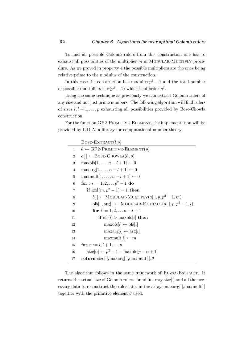
62 Chapter 6. Algorithms for near optimal Golomb rulers
To find all possible Golomb rulers from this construction one has to
exhaust all possibilities of the multiplier m in Modular-Multiply proce-
dure. As we proved in property 4 the possible multipliers are the ones being
relative prime to the modulus of the construction.
In this case the construction has modulus p2 − 1 and the total number
of possible multipliers is φ(p2 − 1) which is of order p2.
Using the same technique as previously we can extract Golomb rulers of
any size and not just prime numbers. The following algorithm will find rulers
of sizes l, l + 1, . . . , p exhausting all possibilities provided by Bose-Chowla
construction.
For the function GF2-Primitive-Element, the implementation will be
provided by LiDIA, a library for computational number theory.
Bose-Extract(l,p)
1 θ ← GF2-Primitive-Element(p)
2 a[ ] ← Bose-Chowla(θ, p)
3 maxofs[1, . . . , n− l + 1] ← 0
4 maxarg[1, . . . , n− l + 1] ← 0
5 maxmult[1, . . . , n− l + 1] ← 0
6 for m := 1, 2, . . . p2 − 1 do
7 if gcd(m, p2 − 1) = 1 then
8 b[ ] ← Modular-Multiply(a[ ], p, p2 − 1,m)
9 ofs[ ], arg[ ] ← Modular-Extract(a[ ], p, p2 − 1, l)
10 for i := 1, 2, . . . n− l + 1
11 if ofs[i] > maxofs[i] then
12 maxofs[i] ← ofs[i]
13 maxarg[i] ← arg[i]
14 maxmult[i] ← m
15 for n := l, l + 1, . . . p
16 size[n] ← p2 − 1−maxofs[p− n + 1]
17 return size[ ],maxarg[ ],maxmult[ ],θ
The algorithm follows in the same framework of Ruzsa-Extract. It
returns the actual size of Golomb rulers found in array size[ ] and all the nec-
essary data to reconstruct the ruler later in the arrays maxarg[ ],maxmult[ ]
together with the primitive element θ used.

6.7. Implementation 63
The running time is now
T2(l, p) = O( φ(p2 − 1))[p log p + p(p− l)] ) (6.3)
Again, by the properties of the Euler’s φ function
T2(l, p) = O( p3 log p + p2(p− l) ) (6.4)
which is worse by a factor p compared to the previous construction.
6.7 Implementation
Both algorithms were implemented in ANSI C++. All the development
was done at the Linux operating system with the GNU C++ compiler. The
source code of both constructions is listed in the appendices.
Since we are dealing with large integers near 232 an important topic that
should be addressed is the possibility of overflowing machine size integers.
Actually, the choice of 65000 as the maximum element of Golomb rulers
co-incides with the limit of 32-bit integers. For p > 65535, p2 overflows 32-bit
integers and would have to resort to arbitrary precision arithmetic libraries.
Then the efficiency of the algorithms would suffer severely by the speed of
these libraries and one should expect the running time to be multiplied by
at least 10, since every elementary operation would be replaced by library
calls.
There are some places in the algorithms that integers of size greater than
p2 have to be computed. Such dangerous places are:
1. Modular-Multiply algorithm line 2, when m · a[i] ≈ p3 if a[i] is
about p2 and the multiplier m is about p.
2. Ruzsa-Extract algorithm line 7, when d is about p2 and g is about
p.
3. Modular-Extract algorithm line 2, where the unwound sequence
might be of size 2p2.
Fortunately, for these limited cases, we use the GNU g++ compiler’s
internal support for fast 64-bit data types (data type long long). We use

64 Chapter 6. Algorithms for near optimal Golomb rulers
such 64-bit integers whenever there is a danger of overflowing 32-bit data
types. To overflow 64-bit integers with p3, p must be at least
p3 > 264 =⇒ p > 2642245
quite above the valus of p we will need to prove 6.1.
The running time of the algorithms is only slightly increased by using
long long carefully and only in places where necessary.
As for the sorting of the sequence, the Sort procedure is an implemen-
tation of standard textbook QuickSort which reverts to insertion sort for
less than 15 elements.
6.8 Exhaustive search for Golomb rulers
To prove theorem 6.1 we have to extract Golomb rulers using the two
consctructions we described for all n 6 65000.
6.8.1 Computing the total running time
Since the algorithms apply only to prime numbers, for each prime less
than 65000 the algorithms should be run and allowed to extract Golomb
rulers down to the previous prime. This will fill the gap between prime
numbers and provide Golomb rulers of all sizes.
For example the first few calls to Ruzsa-Extract will be
Ruzsa-Extract(2, 3)
Ruzsa-Extract(3, 5)
Ruzsa-Extract(5, 7)
Ruzsa-Extract(7, 11)
. . .
Ruzsa-Extract(pn−1, pn)
where pn be the n-th prime. Then the total running time of the Ruzsa
extract algorithm to extract all Golomb rulers of sizes up to x will be by
equation 6.1
T3(x) = O
(pn<x∑
n=1
φ(pn − 1)[pn log pn + pn(pn − pn−1)]
)

6.8. Exhaustive search for Golomb rulers 65
The difference between two consecutive primes pn−pn−1, although com-
pletely irregular, averagely is so slowly increasing that computationally it is
practically constant. So, the second term in the parenthesis is about pn and
neglible to the first term.
T3(x) = O
(pn<x∑
n=1
φ(pn − 1)pn log pn
)
Similarly for the Bose construction the total running time will be
T4(x) = O
(pn<x∑
n=1
φ(p2n − 1)pn log pn
)
Since the sums cannot be evaluated due to the inability to find the
exact distribution of primes, an initial test was run of both algorithms for
x < 3000. Running times are presented for both algorithms in figure 6.8.1.
The running times appear irregular because of the irregularities of the
Euler’s φ functions. However, in the long term the running times follow an
polynomial increase which is of the order n2 for Ruzsa and n3 for Bose. The
running time of Bose appear a bit more regular.
As expected Ruzsa’s construction is much faster than Bose.
T3(x) and T4(x), the cumulative sum of the running times, fitted with a
non-linear curve fitter to the following values
Ruzsa-Extract T3(x) ≈ 5.56 · 10−9x3
Bose-Extract T4(x) ≈ 2.40 · 10−9x4
For x = 65000, Ruzsa-Extract would take about 17 days on the ref-
erence cpu machine and Bose-Extract about 1358 years so the choice of
Ruzsa’s construction as our main tool is inevitable.
The algorithm was run on a computer network of 10 machines. Since
the computations can be split in small units, one for each prime number,
the algorithm parallelizes easily.
A distributed client was implemented which reads a stub (work unit)
from a central server. It then computes the stub and sends the results back
to the server. The communication was done using TCP sockets.
Both client and server were implemented in TCL, which facilitates the
quick development of such application. The workhorse routine was imple-
mented in C++ using GNU C++ compiler.

66 Chapter 6. Algorithms for near optimal Golomb rulers
6.9 Summary
In this chapter we introduced the goal of chapters 6 and 7: the com-
putational verification that Golomb rulers of size less than n2 exist for all
n 6 65000. We have chosen the algorithm which uses Ruzsa’s construc-
tion, having the other algorithm as a backup. In the next chapter, we will
see that this backup, the algorithm for Bose’s construction, will actually be
desperately needed to complete our goal.

6.9. Summary 67
Ruzsa-Extract
0 500 1000 1500 2000 2500 3000n
0
0.5
1
1.5
2
2.5
3
seco
nds
Bose-Extract
0 500 1000 1500 2000 2500 3000n
0
500
1000
1500
2000
2500
3000
seco
nds
Figure 6.1: Running times of both algorithms for the test run

68 Chapter 6. Algorithms for near optimal Golomb rulers
Ruzsa-Extract
0 1000 2000 3000n
0
50
100
150
seco
nds
Bose-Extract
0 1000 2000 3000n
0
50000
100000
150000
200000
seco
nds
Figure 6.2: Cumulative running times of both algorithms

Chapter 7
Results and proof of main
theorem
Computations were carried out first by Ruzsa-Extract for up to 65000
marks. Most of the rulers produced had the desired property of having
length less than n2. However is a small number of cases the best rulers
found had size more than n2. In these cases, the much slower algorithm
Bose-Extract was used to correct the situation and find suitable Golomb
rulers.
7.1 Rulers found by Ruzsa’s construction
First we will consider the much faster construction of Ruzsa and the
algorithm Ruzsa-Extract we developed in the previous chapter.
Computation of Ruzsa’s construction for all rulers up to 65000 number of
marks has been carried out in a distributed network consisting of 10 personal
computers running linux. The computational power of these workstations
varied but most of them had CPU clocks about 1.5GHz.
About 2.1 million cpu seconds or 24 cpu days were used for these com-
putations, close to the estimate of the previous chapter.
7.1.1 Prime number of marks
We will first present the results for prime number of marks in which the
algorithm had no problem to find near-optimal ruler of suitable sizes. In
69
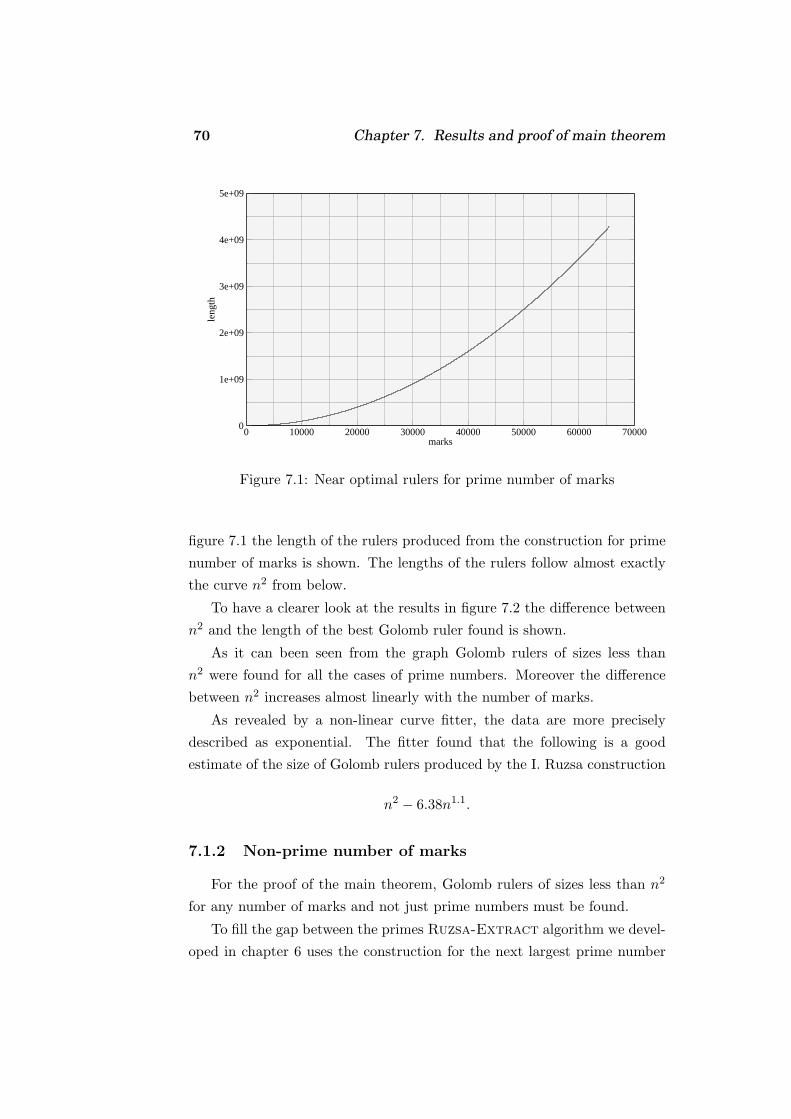
70 Chapter 7. Results and proof of main theorem
0 10000 20000 30000 40000 50000 60000 70000marks
0
1e+09
2e+09
3e+09
4e+09
5e+09
leng
th
Figure 7.1: Near optimal rulers for prime number of marks
figure 7.1 the length of the rulers produced from the construction for prime
number of marks is shown. The lengths of the rulers follow almost exactly
the curve n2 from below.
To have a clearer look at the results in figure 7.2 the difference between
n2 and the length of the best Golomb ruler found is shown.
As it can been seen from the graph Golomb rulers of sizes less than
n2 were found for all the cases of prime numbers. Moreover the difference
between n2 increases almost linearly with the number of marks.
As revealed by a non-linear curve fitter, the data are more precisely
described as exponential. The fitter found that the following is a good
estimate of the size of Golomb rulers produced by the I. Ruzsa construction
n2 − 6.38n1.1.
7.1.2 Non-prime number of marks
For the proof of the main theorem, Golomb rulers of sizes less than n2
for any number of marks and not just prime numbers must be found.
To fill the gap between the primes Ruzsa-Extract algorithm we devel-
oped in chapter 6 uses the construction for the next largest prime number

7.1. Rulers found by Ruzsa’s construction 71
0 10000 20000 30000 40000 50000 60000marks
0
5e+05
1e+06
1.5e+06
2e+06
diff
eren
ce o
f le
ngth
to n
^2
Figure 7.2: Difference of n2 and ruler size for prime number of marks
and removes the necessary number of marks.
The difference of the length and n2 is shown in figures 7.3, 7.4, 7.5 and
7.6.
The algorithm produced good Golomb rulers for the 99.999% of the cases.
However, there is a small number of negative results, in which the length
of the best Golomb ruler produced was more than the goal n2. These cases
have to be resolved for the proof of the main theorem. The results that were
negative are shown in table 7.1.
The problem occurs precisely at the points where the difference between
two consecutive prime numbers is large. In this case the algorithm has to
use a construction for the next largest prime and remove a large number of
elements to fill the gap.
The elements of a dense Golomb ruler are approximately linearly dis-
tributed over the full length of the ruler [23]. That means that starting with
a ruler with n marks and size about n2 the i-th element is about at position
in. Extracting from this ruler another one with m marks, the latter will
have size about mn. Thus, as m decreases, mn becomes increasingly larger
than the goal m2.
This is shown in figure 7.7 where the construction of Ruzsa for 277 marks

72 Chapter 7. Results and proof of main theorem
0 200 400 600 800 1000marks
0
5000
10000
15000
20000
diff
eren
ce o
f le
ngth
to n
^2
Figure 7.3: Near optimal rulers for any number of marks (1-1000)
1000 1500 2000 2500 3000 3500 4000marks
0
20000
40000
60000
80000
diff
eren
ce o
f le
ngth
to n
^2
Figure 7.4: Near optimal rulers for any number of marks (1000-4000)

7.1. Rulers found by Ruzsa’s construction 73
5000 10000 15000 20000 25000 30000marks
0
200000
400000
600000
800000
diff
eren
ce o
f le
ngth
to n
^2
Figure 7.5: Near optimal rulers for any number of marks (4000-30000)
35000 40000 45000 50000 55000 60000 65000marks
-500000
0
500000
1000000
1500000
2000000
diff
eren
ce o
f le
ngth
to n
^2
Figure 7.6: Near optimal rulers for any number of marks (30000-65000)

74 Chapter 7. Results and proof of main theorem
Table 7.1: Negative results
n l n2 − l
113 12790 -211327 1766741 -58121328 1767716 -41321329 1768457 -22161330 1769309 -409
19609 384597182 -8430119610 384624625 -7252519611 384641715 -5039419612 384667800 -3725619613 384686390 -1662125474 648928604 -392831397 986197070 -42546131398 986204645 -37024131399 986296027 -39882631400 986343472 -38347231401 986373159 -35035831402 986424378 -33877431403 986452244 -30383531404 986479109 -26789331405 986542983 -26895831406 986635350 -29851431407 986663424 -26377531408 986677530 -21506631409 986716601 -19132031410 986785033 -19693331411 986820402 -16948131412 986869510 -15576631413 986910763 -13419431414 986943786 -10439031415 986979155 -7693031416 987012077 -4702131417 987031261 -337234061 1160519170 -36744934062 1160547296 -32745234063 1160578879 -29091034064 1160592347 -236251
n l n2 − l
34065 1160623930 -19970534066 1160670148 -17779234067 1160695738 -13524934068 1160696903 -6827934069 1160722604 -2584334070 1160829254 -6435434071 1160953336 -12029534072 1160954501 -5331734073 1160980202 -1087334074 1161037977 -50135617 1268691836 -12114735618 1268720119 -7819535619 1268726764 -1360335623 1269001983 -385440639 1651703022 -17470140640 1651754919 -14531940641 1651757563 -6668240642 1651859670 -8750640643 1651867536 -1408743331 1877839745 -26418443332 1877870808 -20858443333 1877934842 -18595343334 1877977590 -14203443335 1878001275 -7905043336 1878044384 -3548844293 1962072520 -20267144294 1962154288 -19585244295 1962171771 -12474644296 1962230373 -9475744297 1962259182 -3497344298 1962330046 -1724244299 1962450197 -4879644300 1962526788 -3678844301 1962615591 -3699045893 2106197458 -30009

7.2. Rulers found by Bose-Chowla construction 75
is used to extract rulers down to 1 mark. The difference of the length and
n2 quickly becomes negative. The negative results occur precisely at the
points where the difference between two primes assumes a large value.
All negative results can be grouped in the areas shown in table 7.2.
Table 7.2: Negative results and prime gaps
negative results prime gap gap length113 113− 127 14
1327− 1330 1327− 1361 3419609− 19613 19609− 19661 52
25474 25471− 25523 5231397− 31417 31397− 31469 7234061− 34074 34061− 34123 6235617− 35623 35617− 35671 5440639− 40643 40639− 40693 5443331− 43336 43331− 43391 6044293− 44301 44293− 44351 58
45893 45893− 45943 50
The average prime gap between 1 and 1500 is 6 and between 1 and 65000
is 10. When this gap becomes quite larger than this, the algorithm is not
able to produce good Golomb rulers.
The most discouraging case is between 31397 and 31417 where the prime
gap is 72, quite above the average, and Golomb rulers found become very
bad. This situation is displayed more precisely in figure 7.8
7.2 Rulers found by Bose-Chowla construction
7.2.1 Finishing the proof of the main theorem
To finish the proof of our theoren, for the points where Ruzsa’s construc-
tion failed, we used Bose-Extract algorithm for precisely the cases where
size of the rulers produced by the first algorithm was negative.
The algorithm was allowed to run until it found a Golomb ruler of suit-
able size and then stopped. Otherwise running through all possible con-
structions of Bose-Chowla even for a single number of marks p would take
many years of CPU time by the estimate of the previous chapter and the

76 Chapter 7. Results and proof of main theorem
0 50 100 150 200 250 300marks
-10000
-5000
0
5000di
ffer
ence
of
leng
th to
n^2
Figure 7.7: Extracted rulers from a 277 marks construction
31400 31500 31600marks
-500000
0
500000
1000000
diff
eren
ce o
f le
ngth
to n
^2
non-primesprimes
Figure 7.8: The situation between 31397 and 31417

7.2. Rulers found by Bose-Chowla construction 77
observations of the speed that the multipliers were exhausted.
The optimal Golomb rulers found using this method are presented in
the following table, along with the irreducible polynomials and primitive
elements used for the computation of the Galois fields.
GF (1132) = 〈69x + 2〉/x2 + 13x + 41 mod 113
n length m n2 − l
113 11647 115 1122
GF (13622) = 〈1220x + 162〉/x2 + 276x + 48 mod 1362
n length m n2 − l
1327 1751426 98711 95031328 1753632 98711 99521329 1756863 29129 93781330 1757303 29129 11597
GF (196612) = 〈12958x + 10688〉/x2 + 6013x + 5403 mod 19661
n length m n2 − l
19609 384199114 3415357 31376719610 384209834 3415357 34226619611 384255276 3415357 33604519612 384280268 12122089 35027619613 384315330 3415357 354439
GF (255232) = 〈11709x + 22179〉/x2 + 9158x + 7230 mod 25523
n length m n2 − l
25474 648887797 20483 36879
GF (313972) = 〈21016x + 14783〉/x2 + 25136x + 23613 mod 31397
n length m n2 − l
31397 985182074 7391 589535

78 Chapter 7. Results and proof of main theorem
GF (314692) = 〈1554x + 29508〉/x2 + 29760x + 9050 mod 31469
n length m n2 − l
31398 985733211 8556871 10119331399 985790592 8556871 10660931400 985835555 8556871 12444531401 985879154 8556871 14364731402 985951670 8556871 13393431403 986001830 8556871 14657931404 986033653 8556871 17756331405 986087575 8556871 18645031406 986108679 8556871 22815731407 986181195 8556871 21845431408 986231379 8556871 23108531409 986279127 8556871 24615431410 986287982 8556871 30011831411 986309474 8556871 34144731412 986366671 8556871 34707331413 986411811 8556871 36475831414 986480862 8556871 35853431415 986503109 8556871 39911631416 986575625 8556871 38943131417 986633006 8556871 394883
GF (341232) = 〈19239x + 16497〉/x2 + 13878x + 14722 mod 34123
n length m n2 − l
34061 1160133938 1045519 1778334062 1160184349 2087299 3549534063 1160286494 450227 147534064 1160328690 444775 2740634065 1160379857 231775 4436834066 1160412101 231775 8025534067 1160520937 163765 3955234068 1160615428 76973 1319634069 1160673088 33721 2367334070 1160702245 33721 6265534071 1160777943 33721 5509834072 1160822990 33721 7819434073 1160852147 33721 11718234074 1161029988 4751 7488

7.2. Rulers found by Bose-Chowla construction 79
GF (356712) = 〈19447x + 33743〉/x2 + 25262x + 26129 mod 35671n length m n2 − l
35617 1268463057 88651 10763235618 1268475498 88651 16642635619 1268703314 71489 984735620 1268760714 71489 2368635621 1268836365 68011 1927635622 1268903019 27589 2386535623 1268976373 4367 21756
GF (406932) = 〈5595x + 16764〉/x2 + 21946x + 2344 mod 40693n length m n2 − l
40639 1651339857 16115 18846440640 1651398771 16115 21082940641 1651504446 16115 18643540642 1651563360 16115 20880440643 1651667503 16115 185946
GF (433912) = 〈39179x + 25402〉/x2 + 4218x + 42993 mod 43391n length m n2 − l
43331 1877499646 84529 7591543332 1877540552 84529 12167243333 1877627142 84529 12174743334 1877771317 84529 6423943335 1877812223 84529 11000243336 1877898813 84529 110083
GF (443512) = 〈3722x + 32899〉/x2 + 1508x + 4745 mod 44351n length m n2 − l
44293 1961850181 380159 1966844294 1961890065 380159 6837144295 1961926018 380159 12100744296 1961965902 380159 16971444297 1962017702 380159 20650744298 1962077915 380159 23488944299 1962257057 380159 14434444300 1962280901 380159 20909944301 1962341114 380159 237487
GF (459432) = 〈2981x + 13885〉/x2 + 34036x + 4658 mod 45943n length m n2 − l
45893 2105954557 97321 212892

80 Chapter 7. Results and proof of main theorem
7.2.2 Complete computations of Bose’s construction
Apart from the proof of the main theorem, Bose-Chowla construction
was completely evaluated iterating through all possible constructions and
multipliers for a number of marks up to 3000 marks.
In this range Bose’s construction has produced in most of the cases
better Golomb rulers that Ruzsa’s construction, of course with much more
computational time. Golomb rulers of sizes less than n2 were found in this
range for any number of marks.
The results for up to 3000 marks are presented in figure 7.9. As usual
the difference between the length and n2 is presented.
The function x√
x is also plotted which was believed by some authors
to be about the difference between n2 and the length of an optimal Golomb
ruler. However, clearly x√
x diverges from the results so the conjecture that
the length of an optimal ruler is about x2 − x√
x does not seem to hold.
7.3 Summary
The algorithms Ruzsa-Extract and Bose-Extract together were
used to provide the proof of the main theorem of chapter 6.
All the results together with the appropriate code and tables of computed
Golomb rulers, can be found at the web page devoted to this diploma thesis
http://www.softnet.tuc.gr/~apdim/diploma.

7.3. Summary 81
0 1000 2000 3000marks
0
20000
40000
60000
80000
diff
eren
ce o
f le
ngth
to n
^2
x*sqrt(x)best ruler found
Figure 7.9: Rulers found by Bose-Chowla for up to 3000 marks

82 Chapter 7. Results and proof of main theorem

Chapter 8
Conclusion
In this thesis, two related problem from number theory, Golomb rulers
and Sidon sets were investigated. Although the two problems are closely
related, they were studied almost independently, with some authors ignoring
and reproving older results.
To clarify this situation, we have concentrated on the equivalence be-
tween the two problems and, in chapter 4, we proved theorems that allow
bounds from one problem to be restated to the other.
The results were applied to a known upper bound on the size of Sidon
sets by Lindstrom to yield a better lower bound for the length of optimal
Golomb rulers: an optimal Golomb ruler must have size at least
n2 − 2n√
n +√
n− 2
In the second part of the thesis, we investigated constructions from num-
ber theory that give modular Golomb rulers and Sidon sets. All the known
constructions were reviewed and we investigated their application to Golomb
rulers. Of more interest are the three constructions by Singer, Bose-Chowla
and Ruzsa. All of these constructions can be applied to produce Golomb
rulers of size near n2, whose length is close to the optimal one (and in some
cases optimal).
A conjecture from Sidon sets, that their size is at most n1/2 is an old
conjecture, circulated by Erdos in the early 40’s. Restating this to Golomb
rulers (using the results of chapter 4), the conjecture reads that the size of
an optimal Golomb rulers is less that n2.
83

84 Chapter 8. Conclusion
In chapter 6, we have developed algorithms that allow the quick eval-
uation of both Ruzsa’s construction and Bose’s construction to yield near-
optimal Golomb rulers. These algorithms, Bose-Extract and Ruzsa-
Extract have been used to computationally prove the main theorem of
chapter 6 and this thesis, that the conjecture of Erdos is true up to a bound
on the number of marks of the ruler.
Both algorithms were used, as Ruzsa’s construction failed to produce
suitable Golom rulers in some cases where there is a large gap between
prime numbers.
Using about 21 CPU days on a distributed run of both algorithms, we
proved that rulers of size less than n2 exist for all n less than 65000. Equiv-
alently, in Sidon set terms
F2(n) < n1/2 for all n < 650002
So, the conjecture of Erdos is true up to 4.225·109. It is still not known if
this holds for all n. However, the search we have done can be extended (with
additional computational power) to larger bounds. Indeed, it appears that
Erdos conjecture is true, however the proof of such a statement is beyond
the reach of today’s mathematical knowledge.

Bibliography
[1] M. Ajtai, J. Kolmos, and E. Szemeredi, A dense infinite Sidon sequence,
European Journal of Combinatorics 2 (1981), 1–11.
[2] N. Alon and M. N. Kolountzakis, On a problem of Erdos and Turan
and some related results, Journal of number theory 55 (1995), 82–93.
[3] Andersson, Hagerup, Nilsson, and Raman, Sorting in linear time?,
STOC: ACM Symposium on Theory of Computing (STOC), 1995.
[4] A. Andersson, T. Hagerup, S. Nilsson, and R. Raman, Sorting in linear
time?, Journal of Computer and System Sciences 57 (1998), 74–93.
[5] M. D. Atkinson, N. Santoro, and J. Urrutia, Integer sets with distinct
sums and differences and carrier frequence assignments for nonlinear
repeaters, IEEE Transactions on Communications 34 (1986), 614–617.
[6] W.C. Babock, Intermodulation interference in radio systems, Bell Sys-
tems Technical Journal (1953), 63–73.
[7] G. S. Bloom and S. W. Golomb, Numbered complete graphs, un-
usual rulers, and assorted applications, Lecture Notes in Mathematics,
Springer-Verlag New York, 1976, pp. 53–65.
[8] , Applications of numbered undirected graphs, Proceedings of
IEEE 65 (1977), 562–571.
[9] E. J. Blum, F. Biraud, and J. C. Ribes, On optimal synthetic linear
arrays with applications to radioastronomy, IEEE Transactions on An-
tennas and Propagation 22 (1974), 108–109.
85

86 BIBLIOGRAPHY
[10] E. J. Blum, J. C. Ribes, and F. Biraud, Some new possibilitied of opti-
mal synthetic linear arrays for radioastronomy, Astronomy and Astro-
physics 41 (1975), 409–411.
[11] R.C. Bose, An affine analogue of Singer’s theorem, Journal of the Indian
Mathematical Society 6 (1942), 1–15.
[12] R.C. Bose and S. Chowla, Theorems in the additive theory of numbers,
Commentarii Mathematici Helvetici 37 (1962-63), 141–147.
[13] Zhi Chen, Further results on difference triangle sets, IEEE Transactions
on Information Theory 40 (1994), 1268–1270.
[14] S. Chowla, Solution of a problem of Erdos in and Turan in additive
number theory, Proceedings of the National Academy of Sciences, India
14 (1944), 1–2.
[15] J. Cilleruelo, Gaps in dense sidon sets, The Electronic Journal of Com-
binatorial Number Theory 0 (2000).
[16] T. Cormen, C. Leiserson, R. Rivest, and C. Stein, Introduction to algo-
rithms, 2nd ed., MIT Press, 2001.
[17] A. K. Dewdney, Computer recreations, Scientific American 253 (1985),
no. 6, 16–20.
[18] , Computer recreations, Scientific American 254 (1986), no. 3,
14.
[19] A. Dollas, W. T. Rankin, and D. McCracken, A new algorithm for
Golomb ruler derivation and proof of the 19 mark ruler, IEEE Trans-
actions on Information Theory 44 (1998), 379–382.
[20] A. R. Eckler, The construction of missile guidance codes resistant to
random interference, Bell System Tech. Journal (1960), 973–994.
[21] P. Erdos, On a problem of Sidon in additive number theory, Acta Sci-
entiarum Mathematicarum, Univ. Szeged 15 (1953-54), 255–259.
[22] P. Erdos and R. Freud, On sums of a sidon-sequence, Journal of Number
Theory 38 (1991), 196–205.

BIBLIOGRAPHY 87
[23] P. Erdos, A. Sarkozy, and V. Sos, On sum sets of Sidon sets I., Journal
of Number Theory 47 (1994), 329–347.
[24] P. Erdos and A. Renyi, Additive properties of random sequences of pos-
itive integers, Acta Arithmetica 6 (1960), 83–110.
[25] P. Erdos and P. Turan, On a problem of Sidon in additive number
theory and some related problems, Journal. of the London Mathematical
Society 16 (1941), 212–215, Addendum (by P. Erdos), ibid. 19(1944),
208.
[26] M. Gardner, Mathematical games, Scientific American (1972), no. 3,
108–112.
[27] S.W. Graham, Bh sequences, Proceedings of a Conference in Honor of
Heine Halberstam, Birkhauser, 1996, pp. 337–355.
[28] Richard K. Guy, Unsolved problems in number theory, 2nd ed., Problem
Books in Mathematics, Unsolved Problems in Intuitive Mathematics, I.,
ch. 10 Modular Difference Sets and Error Correcting Codes, Springer-
Verlag, New York, 1994.
[29] H. Halberstam and K. F. Roth, Sequences, vol. I, Oxford University
Press, 1966, (2nd ed. Springer-Verlag, New York, 1983).
[30] G. H. Hardy and E. M. Wright, An introduction to the theory of num-
bers, 5th ed., Oxford University Press, 1989.
[31] M. Helm, Some remarks on the Erdos-Turan conjecture, Acta arith-
metica 63 (1993), 373–378.
[32] X.-D. Jia, On finite Sidon sequences, Journal of number theory 44
(1993), 84–92.
[33] Martin Klazar, Note on the maximum size of a Sidon set, unpublished.
[34] E. J. Klieber, Some difference triangles for constructing self-orthogonal
codes, IEEE Transactions on Information Theory 16 (1970), 237–238.
[35] T. Kløve, Bounds on the size of optimal difference sets, IEEE Transac-
tions on Information Theory 34 (1988), 355–361.

88 BIBLIOGRAPHY
[36] , Bounds and construction for difference triangle sets, IEEE
Transactions on Information Theory 35 (1989), 879–886.
[37] D. E. Knuth, The art of computer programming. volume 2: Seminu-
merical algorithms, Addison-Wesley, 1969.
[38] Mihail N. Kolountzakis, Probabilistic and constructive methods in har-
monic analysis and additive number theory, Ph.D. thesis, Stanford Uni-
versity, May 1994.
[39] , On the uniform distribution in residue classes of dense sets
of integers with distinct sums, Journal of number theory 76 (1999),
147–153.
[40] A. W. Lam and D. V. Sarwate, On optimum time-hopping patterns,
IEEE Transactions on Communications 36 (1988), 380–382.
[41] R. Lidl and H. Niederreiter, Finite fields, Encyclopedia of Mathematics,
vol. 20, Cambridge University Press, 1997.
[42] Bernt Lindstrom, An inequality for b2-sequences, Journal of Combina-
torial Theory 6 (1969), 211–212.
[43] , Finding finite B2-sequences faster, Mathematics of Computa-
tion 67 (1998), 1173–1178.
[44] , Well distribution of Sidon sets in residue classes, Journal of
Number Theory 69 (1998), 197–200.
[45] R. Lorentzen and R. Nilsen, Application of linear programming to the
optimal difference triangle set problem, IEEE Transactions on Informa-
tion Theory 37 (1991), 1268–1270.
[46] William T. Rankin, Optimal Golomb rulers: An exhaustive parallel
search implementation, Master’s thesis, Duke University, department
of Electrical Engineering, 1993.
[47] J. Robinson and A. Bernstein, A class of binary recurrent codes with
limited error propagation, IEEE Transactions on Information Theory
13 (1967), 106–113.

BIBLIOGRAPHY 89
[48] J. P. Robinson, Optimal Golomb rulers, IEEE Transactions on Com-
puters 28 (1979), 943–944.
[49] , Addendum to optimal Golomb rulers, IEEE Transactions on
Computers 32 (1983), 201.
[50] Imre Z. Ruzsa, Solving a linear equation in a set of integers I, Acta
Arithmetica LXV.3 (1993), 259–282.
[51] J. B. Shearer, Some new optimum Golomb rulers, IEEE Transactions
on Information Theory 36 (1990), 183–184.
[52] S. Sidon, Mathematische Annalen 106 (1932), 539.
[53] J. Singer, A theorem in finite projective geometry and some applications
to number theory, Transactions of the American Mathematical Society
43 (1938), 377–385.
[54] Zhenxiang Zhang, Finding finite B2-sequences with larger m − a1/2m ,
Mathematics of Computation 63 (1994), 403–414.
[55] C. Zhi, F. Pingzhi, and J. Fan, Disjoint difference sets, difference tri-
angle sets and related codes, IEEE Transactions on Information Theory
38 (1992), 518–522.

90 BIBLIOGRAPHY

Appendix A: Source code
1 ruzsa.C
#define REVISION 1 . 3 5
/∗5 This program w i l l f i nd the best p o s s i b l e Golomb ru l e r
f o r p prime us ing Ruzsa con s t ru c t i on .
Usage :. / f i n d a l l l p
10
Var ia t i on s : −DCHECK −> check i f the produced r u l e r sare a c t ua l l y golomb .
p must be prime . I t w i l l f i nd a l l golomb r u l e r s o f s i z e s15 l . . p−1 us ing the con s t ru c t i on f o r p .
∗/
20 typedef long long i n t64 ;typedef unsigned int uint32 ;typedef unsigned int myint ; // datatype f o r the s o r t
#include < i o s t ream . h>25 #include <math . h>
#include < s t d l i b . h>#include < s t d i o . h>#include < time . h>#include < s i g n a l . h>
30 #include <uni s td . h>
uint32 a [ 2 3 0 0 0 0 ] ;
#include ”common .C”35
/∗Function : g ene ra t e one l i nd s t r om ( g , p , f )
Compute the Sidon s e t us ing Lindstrom cons t ruc t i on f o r
91

92 Appendix A: Source code
40 parameters g , p , f
∗/
void45 gene ra t e one l i nd s t r om ( uint32 g , u int32 p , u int32 f , u int32 a [ ] ){
uint32 c = p∗ f ;i n t64 d = (p−1)∗g ;
50 uint32 z = p∗(p−1);
for ( u int32 i =1; i<=p−1; i++){
i n t64 m = ( c + d) % z ;55
a [ i ] = m;
c += p∗ f ;d = (d∗g ) % z ;
60 }}
/∗Function : genera te one ( g , p)
65
Compute the Sidon s e t us ing I . Ruzsa con s t ru c t i on f o rparameters g , p
∗/
70
voidgenerate one ( u int32 g , u int32 p , u int32 f , u int32 a [ ] ){
uint32 c = p ;75 i n t64 d = (p−1)∗g ;
u int32 z = p∗(p−1);
for ( u int32 i =1; i<=p−1; i++){
80 i n t64 m = ( c + d) % z ;
a [ i ] = m;
c += p ;85 d = (d∗g ) % z ;
}}
90 long long o f s [ 1 0 0 0 0 ] ;u int32 arg [ 1 0 0 0 0 ] ;
/∗

1. ruzsa.C 93
Function : modular extract ( a , n , p , l )95
For sequence a [ i ] f i nd a l l maximum o f f s e t sby t runcat ing down to l e lements
∗/
100 /∗ DO SOME PREPROCESSING TO SPEED THINGS UP:a [ n + 1 ] . . . a [ 2 n] <− a [1 ]+p . . . a [ n]+p
∗/
long long b [ 1 5 0 0 0 0 ] ; /∗ the unwound sequence ∗/105
void modular extract ( u int32 a [ ] , u int32 n , u int32 z , u int32 l ){
uint i , j , k ;
110 for ( i =1; i<=n ; i ++) { b [ i ] = a [ i ] ; b [ n+i ] = ( long long ) a [ i ]+z ; }
for ( i =1; i<=n−l +1; i ++) o f s [ i ] = 0 ;
for ( k=1; k<=n−l +1; k++)115 #i f d e f BREAK
i f ( min length [ n−k+1] > (n−k+1)∗(n−k+1))#end i f
for ( i =1; i<=n ; i++){
120 long long do f s = b [ i+k ] − b [ i ] ;
i f ( do f s > o f s [ k ] ){
o f s [ k ] = do f s ;125 arg [ k ] = i+k ;
}}
for ( i =1; i<=n−l +1; i ++) i f ( arg [ i ] > n ) arg [ i ] −= n ;130 }
/∗Fucntion : f i n d b e s t ( i n t b [ ] , i n t a [ ] , i n t p , i n t z )
135 Print the best r u l e r found with ( p−z ) e lementsa f t e r maximum o f f s e t s has foundthe best s h i f t . Store in b [ ]
∗/140
void f i n d b e s t ( long long b [ ] , long long a [ ] , u int32 p , u int32 z ){
uint32 j = arg [ z ] ;u int32 o f s = a [ j ] ;
145
for ( u int32 i =1; i<=p−z+1; i ++) b [ i ] = a [ j ++] − o f s ;}

94 Appendix A: Source code
150 /∗i n t FindAll ( r , p ) :
g iven an i n t e g e r r a c t ua l l y f i nd the best r u l e r s withr , r + 1 , . . . , p−1 marks
155 by t runcat ing the con s t ru c t i on f o r prime p a f t e r .
Return s u i t a b l e a r rays max ofs , max mult , gused f o r the c on s t ru c t i on s .
160 Do not a c t ua l l y f i nd the r u l e r s .∗/
uint32 max ofs [ 1 0 0 0 ] , max mult [ 1 0 0 0 ] , max arg [ 1 0 0 0 ] ;u int32 g ;
165
void r u z s a ex t r a c t ( u int32 l , u int32 p){
for ( u int i =1; i<=p−l ; i ++) max ofs [ i ] = 0 ;
170 uint32 f = 1 ;
/∗ f i nd a p r im i t i v e element ∗/uint32 g1 = 1 ;while ( ! i s p r i m i t i v e ( g1 , p ) ) g1++;
175
g = g1 ;
// f o r ( u int32 t =1; t<p−1; t++,g=(g∗g1)%p ) i f (mygcd( t , p−1)==1)
180 uint32 a0 [ 2 3 0 0 0 0 ] ;genera te one ( g , p , 1 , a0 ) ;
/∗ No need to vary prim . element s i n c e i tproduces the same r u l e r s ! ! ∗ /
185
for ( u int m=1;m<=p−1;m++) i f (mygcd(m, p−1)==1){
/∗ Modular−Mult ip ly ∗/for ( u int i =1; i<=p−1; i++)
190 a [ i ] = ( ( long long )m∗a0 [ i ] ) % (p∗(p−1)) ;
s o r t ( a , p−1);
modular extract ( a , p−1,p∗(p−1), l ) ;195
for ( int i =1; i<=p−l ; i++)i f ( o f s [ i ] > max ofs [ i ] ){
max ofs [ i ] = o f s [ i ] ;200 max mult [ i ] = m;

1. ruzsa.C 95
#i f d e f CHECKlong long b1 [ 7 0 0 0 0 ] ;f i n d b e s t ( b1 , b , p−1, i ) ;
205 cout << i << ” :” ;for ( int l =1; l<=p−i ; l ++) cout << b1 [ l ] << ” ” ;
cout << ”(” << i s go lomb (b1 , p−i ) ;
210 i f ( i s go lomb (b1 , p−i ) !=1){ cout << ” e r r o r \n” ; e x i t ( 1 ) ; }
cout << ”)\n” ;#end i f
215 }}
}
uint l , p ;220
int main ( int argc , char ∗ argv [ ] ){
c e r r << ”RuzsaFind ( f a s t ) rev ” << REVISION << ”\n\n” ;
225 i f ( argc != 3 ){
c e r r << ”\bUsage : ruzsa l p\n\n” ;e x i t ( 1 ) ;
}230
l = a t o i ( argv [ 1 ] ) ;p = a t o i ( argv [ 2 ] ) ;
235
#i f d e f LASTPRIMEl = p−1;while ( ! i s p r ime ( l ) ) l−−;#end i f
240
i f ( ! i s p r ime (p ) ){
c e r r << p << ” i s not a prime number !\n” ;e x i t ( 1 ) ;
245 }
r u z s a ex t r a c t ( l , p ) ;
f p r i n t f ( s t d e r r ,”%d %.3 f s ec \n” , p , usert ime ( ) ) ;250
for ( int n=l ; n<p ; n++)cout << n << ” ” << p∗(p−1)−max ofs [ p−n] << ” ”
<< p << ” ” << g << ” ” << max mult [ p−n] << ”\n” ;
255 f f l u s h ( stdout ) ;

96 Appendix A: Source code
return 0 ;}

2. bose-fast.C 97
2 bose-fast.C
#define REVISION 2 . 2 2
/∗5 Find r u l e r s us ing Bose−Chowla con s t ruc t i on
Usage :. / bose−f a s t l p
10 p must be prime . I t w i l l f i nd a l l golomb r u l e r s o f s i z e sl . . p us ing the con s t ru c t i on f o r p .
Compile :g++−O2 bose−f a s t .C −lLiDIA −lgmp −lm
15
Needs LiDIA l i b r a r y f o r number theory( see http ://www. in fo rmat ik . tu−darmstadt . de/TI/LiDIA/)
Var i a t i on s :20 −DCHECK −> check i f the produced r u l e r s
are a c t ua l l y golomb .−DBREAK −> stop s e r ch ing when golomb r u l e r s o f
s i z e l e s s than nˆ2−2n are found .∗/
25
#include < i o s t ream . h>#include < f s t ream . h>#include < s t r s t r eam . h>#include < s t r i n g . h>
30 #include < s t d l i b . h>#include < s i g n a l . h>#include < time . h>#include <uni s td . h>
35 #include <LiDIA/ b i g i n t . h>#include <LiDIA/ g f e l ement . h>#include <LiDIA/ timer . h>
typedef unsigned long int myint ;40 typedef unsigned long int uint32 ;
long long o f s [ 1 0 0 0 0 ] ;u int32 arg [ 1 0 0 0 0 ] ;
45
/∗ Mininum data found ∗/long long min length [ 1 0 0 0 0 0 ] ;long long min mult [ 1 0 0 0 0 0 ] ;
50 int cu r r en t s t a t e ;
u int m, i ;

98 Appendix A: Source code
char fname [ 2 5 6 ] , f i e ldname [ 2 5 6 ] ;55
#include ”common .C”
/∗60 Function : modular extract ( a , n , p , l )
For sequence a [ i ] f i nd a l l maximum o f f s e t sby t runcat ing down to l e lements
∗/65
/∗ DO SOME PREPROCESSING TO SPEED THINGS UP:a [ n + 1 ] . . . a [ 2 n] <− a [1 ]+p . . . a [ n]+p
∗/
70 long long b [ 2 5 0 0 0 0 ] ; /∗ the unwound sequence ∗/
void modular extract ( u int32 a [ ] , u int32 n , u int32 z , u int32 l ){
uint i , j , k ;75
for ( i =1; i<=n ; i ++) { b [ i ] = a [ i ] ; b [ n+i ] = ( long long ) a [ i ]+z ; }
for ( i =1; i<=n−l +1; i ++) o f s [ i ] = 0 ;
80 for ( k=1; k<=n−l +1; k++)#i f d e f BREAKi f ( min length [ n−k+1] > (n−k+1)∗(n−k+1))#end i f
for ( i =1; i<=n ; i++)85 {
long long do f s = b [ i+k ] − b [ i ] ;
i f ( do f s > o f s [ k ] ){
90 o f s [ k ] = do f s ;arg [ k ] = i+k ;
}}
95 for ( i =1; i<=n−l +1; i ++) i f ( arg [ i ] > n ) arg [ i ] −= n ;}
100 /∗Fucntion : f i n d b e s t ( i n t b [ ] , i n t a [ ] , i n t p , i n t z )
Pr int the best r u l e r found with ( p−z ) e lementsa f t e r maximum o f f s e t s has found
105 the best s h i f t . Store in b [ ]
∗/
2. bose-fast.C 99
void f i n d b e s t ( myint b [ ] , myint a [ ] , u int n , u int z )110 {
uint j = arg [ z ] ;myint o f s = a [ j ] ;
for ( u int i =1; i<=n−z+1; i ++) b [ i ] = a [ j ++] − o f s ;115 }
120 struct poly { long int d [ 3 ] ; void pr in t (void ) ; } ;
voidpoly : : p r i n t (void ){
125 cout << d [2 ] << ” xˆ2 + ” ;cout << d [1 ] << ” x + ” ;cout << d [0 ] << ” ” ;cout << ”\n” ;
}130
poly i r r e d , prim ;
int mod ; /∗ mod = p ∗/
135
/∗Mult ip ly two polynomia l s o f degree at most 1 and reducemodulo an i r r e d u c i b l e poly o f degree 2
140 The i r r e d u c i b l e polynomial i s assumed tohave l ead ing c o e f f 1
∗/
poly145 poly mul ( poly a , poly b)
{poly r ;
r . d [ 0 ] = ( a . d [ 0 ] ∗ b . d [ 0 ] ) % mod ;150 r . d [ 1 ] = ( a . d [ 1 ] ∗ b . d [ 0 ] + a . d [ 0 ] ∗ b . d [ 1 ] ) % mod ;
r . d [ 2 ] = ( a . d [ 1 ] ∗ b . d [ 1 ] ) % mod ;
int c = r . d [ 2 ] ;
155 r . d [0 ] −= c ∗ i r r e d . d [ 0 ] ;r . d [1 ] −= c ∗ i r r e d . d [ 1 ] ;r . d [ 2 ] = 0 ;
/∗ r . d [ 2 ] w i l l be 0 ∗/160 // r . d [2 ] −= c ∗ i r r e d . d [ 2 ] ;

100 Appendix A: Source code
r . d [0 ] %= mod ;r . d [1 ] %= mod ;
165 i f ( r . d [ 0 ]<0 ) r . d [0 ] += mod ;i f ( r . d [ 1 ]<0 ) r . d [1 ] += mod ;
return r ;}
170
using namespace LiDIA ;
Fp polynomial min polynom [ 1 0 0 0 0 0 ] ;175 Fp polynomial f i e l d p o l y ;
myint a [ 1 2 0 0 0 0 ] , a0 [ 1 2 0 0 0 0 ] ;u int n=0;
180
/∗Generate the Bose−Chowla f i e l d pˆ2 in to a0 [ 1 . . n ]
∗/
185 void generate ( u int p){
g a l o i s f i e l d f i e l d ( ( long int )p , 2 ) ;
f i e l d p o l y = f i e l d . i r r ed po l ynomia l ( ) ;190
#i f d e f DEBUGcout << ”Generating f i e l d GF∗(” << p << ” ˆ 2 ) . . . \ n\n” ;
195 cout << ”This f i e l d has ” ;cout << f i e l d . number of e lements ( ) ;cout <<” e lements .\n” ;#end i f
200 #i f d e f DEBUGcout << ”The d e f i n i n g polynomial o f the f i e l d i s \n” ;cout << f i e l d p o l ycout << endl ;#end i f
205
g f e l ement th ( f i e l d ) , elem ( f i e l d ) ;
elem . a s s i g n p r im i t i v e e l emen t ( f i e l d ) ;
210 cout << ”A pr im i t i v e element i s : ” << elem << ”\n” ;cout << ”Order o f element i s : ” << elem . order () << ”\n” ;
th = elem ;
215 Fp polynomial fp = f i e l d p o l y ;

2. bose-fast.C 101
( ( b i g i n t ) fp [ 0 ] ) . l o n g i f y ( i r r e d . d [ 0 ] ) ;( ( b i g i n t ) fp [ 1 ] ) . l o n g i f y ( i r r e d . d [ 1 ] ) ;( ( b i g i n t ) fp [ 2 ] ) . l o n g i f y ( i r r e d . d [ 2 ] ) ;
220
fp = elem . po lynomia l rep ( ) ;
( ( b i g i n t ) fp [ 0 ] ) . l o n g i f y ( prim . d [ 0 ] ) ;( ( b i g i n t ) fp [ 1 ] ) . l o n g i f y ( prim . d [ 1 ] ) ;
225 ( ( b i g i n t ) fp [ 2 ] ) . l o n g i f y ( prim . d [ 2 ] ) ;
i f ( i r r e d . d [ 2 ] ! = 1 ){
cout230 << ” i r r e d u c i b l e has not so good l ead ing c o e f f f i c i e n t \n” ;
e x i t ( 1 ) ;}
235 cu r r en t s t a t e = 1 ;
poly theta = prim ;mod = p ;
240 n=0;
for ( i =1; i<p∗p ; i++){
i f ( theta . d [ 1 ] − prim . d [ 1 ] == 0) a0[++n ] = i ;245
theta = poly mul ( theta , prim ) ;}
i f (n != p ) { cout << ” e r r o r ! n=” << n << ”\n” ; e x i t ( 1 ) ; }250
ofstream of ( f i e ldname ) ;
o f << ” F i e ld : ” << p << ”ˆ2\n” ;o f << ” I r r e d u c i b l e polynomial : ” << f i e l d p o l y << ”\n” ;
255 o f << ” Pr imi t ive element : ” << elem << ”\n” ;o f << ”\n” ;
for ( int i =1; i<=p ; i ++) o f << a0 [ i ] << ”\n” ;}
260
/∗Compute a l l r u l e r s o f s i z e s l . . . p
∗/265
voidcompute ( u int l , u int p){
i f s t r e am f i e l d i n ( f i e ldname ) ;

102 Appendix A: Source code
270
i f ( f i e l d i n ){
cout << ”\nReading f i e l d from ” << f i e ldname << ”\n” ;
275 char t [ 5 0 0 ] ;f i e l d i n . g e t l i n e ( t , 5 0 0 ) ;f i e l d i n . g e t l i n e ( t , 5 0 0 ) ;f i e l d i n . g e t l i n e ( t , 5 0 0 ) ;f i e l d i n . g e t l i n e ( t , 5 0 0 ) ;
280
n=0;for ( int i =1; i<=p ; i ++) f i e l d i n >> a0[++n ] ;
cout << ” F i e ld : ” << a0 [ 1 ]285 << ” ” << a0 [2 ] << ” . . . ” << a0 [ n] << ”\n” ;
}else{
generate (p ) ;290 }
#i f d e f CHECKint i s = is go lomb ( a0 , n ) ;cout << ”\n” ;
295 cout << ” i s go lomb : ” << i s << ”\n” ;
i f ( i s ==0) { cout << ” e r r o r ! ” ; e x i t ( 1 ) ; }#end i f
300 cout << ”Varying f to produce new r u l e r s . . . \ n” ;c u r r en t s t a t e = 2 ;
for (m=1;m<=p∗p−1;m++) i f ( mygcd(m, p∗p−1) == 1 ) {
305 /∗ Modular−Mult ip ly by m∗/for ( u int i =1; i<=n ; i++)
a [ i ] = ( ( ( long long )m)∗ a0 [ i ] ) % ( p∗p−1);
s o r t ( a , n ) ;310
modular extract ( a , n , p∗p−1, l ) ;
for ( u int n=l ; n<=p ; n++){
315 uint d =(p∗p−1−o f s [ p−n +1 ] ) ; /∗ l ength o f r u l e r computed ∗/
#i f d e f CHECKint j = arg [ p−n+1] ;
320 myint s h i f t = a [ j ] ;
myint b [ 1 2 0 0 0 0 ] ;for ( int i =1; i<=n ; i ++) b [ i ] = a [ j++]− s h i f t ;
2. bose-fast.C 103
325 // cout << n << ” : ” ;// cout << ”( ” << i s go lomb (b , n) << ”) ” ;// p r i n t (b , n ) ;
i f ( ! i s go lomb (b , n ) ) { cout << ” e r r o r \n” ; e x i t ( 1 ) ; }330 #end i f
i f (d < min length [ n ] ){
min length [ n ] = d ;335 min mult [ n ] = m;
}} // n
/∗ Break the loop i f we found a l l r u l e r s340 with s i z e s l e s s than n∗n ∗/
#i f d e f BREAKuint n ;for (n=l ; n<=p ; n++) i f ( min length [ n]>=(long long )n∗n ) break ;
345 i f (n>p ) break ;#end i f
} // m}
350
uint l , u ;
355 /∗ pr in t r e s u l t s so f a r ∗/void qu i t ( int t ){{
ofstream out ( fname ) ;360
for ( long long t=l ; t<=u ; t++)out<< t << ” ”<< min length [ t ] << ” ”
365 << min mult [ t ] << ” ”<< ( t ∗ t−(signed long long ) min length [ t ]) << ”\n” ;
out . c l o s e ( ) ;}
370
i f ( c u r r en t s t a t e == 1)cout << ”Computing f i e l d i=” << i << ”/” << u∗u << ”\n” ;
else{
375 cout << ”Modular mult ip ly m=” << m << ”/”<< u∗(u−1) << ”\n” ;

104 Appendix A: Source code
for ( long long t=l ; t<=u ; t++)cout
380 << t << ” ”<< min length [ t ] << ” ”<< min mult [ t ] << ” ”<< ( t ∗ t−(signed long long ) min length [ t ]) << ”\n” ;
385 cout << ”\n” ;}
}
390 int main ( int argc , char ∗ argv [ ] ){
cout << ”Bose−Chowla ( f a s t ) rev ” << REVISION << ”\n\n” ;
l = a t o i ( argv [ 1 ] ) ;395 u = a to i ( argv [ 2 ] ) ;
i f ( argc != 3 ){
cout << ”usage : bose−f a s t l u\n\n” ;400 e x i t ( 1 ) ;
}
#i f d e f LASTPRIMEl = u−1;
405 while ( ! i s p r ime ( l −1)) l−−;#end i f
i f ( ! i s p r ime (u ) ){
410 c e r r << u << ” i s not a prime number !\n” ;e x i t ( 1 ) ;
}
s p r i n t f ( fname , ” outquick%d . dat” , u ) ;415 s p r i n t f ( f i e ldname , ” g f r u l e r%d . dat” , u ) ;
p r i n t f ( ” Construct ing Bose f o r %d” ) ;p r i n t f ( ” and t runcat ing down to %d\n” , u , l ) ;
420 for ( u int i=l ; i<=u ; i ++) min length [ i ] = ( long long )1<<40;
s i g n a l (SIGINT , qu i t ) ;
compute ( l , u ) ;425
p r i n t f (”%d %.3 f \n” , u , usert ime ( ) ) ;
/∗ Write r e s u l t s ∗/
430 for ( long long t=l ; t<=u ; t++)cout

2. bose-fast.C 105
<< t << ” ”<< min length [ t ] << ” ”<< min mult [ t ] << ” ”
435 << ( t ∗ t−(signed long long ) min length [ t ]) << ”\n” ;
o fstream out ( fname ) ;
for ( long long t=l ; t<=u ; t++)440 out
<< t << ” ”<< min length [ t ] << ” ”<< min mult [ t ] << ” ”<< ( t ∗ t−(signed long long ) min length [ t ]) << ”\n” ;
445
out . c l o s e ( ) ;
cout . f l u s h ( ) ;}

106 Appendix A: Source code
3 common.C
/∗Functions : i s go lomb (n , a [ ] )
5 Check i f g iven s e t i s a golomb ru l e r in time O(nˆ2)
assume that a [ i ] are so r t ed∗/
10 char ∗ d i s t = new char [ 1 6 0 00000 ] ;
template<class myint>int i s go lomb ( myint a [ ] , u int n){
15 // uint32 d i s t [ 1 0 0 0 0 0 0 ] ;
d i s t [ 0 ] = 1 ;for ( u int i =1; i<=a [ n ] ; i ++) d i s t [ i ] = 0 ;
20 for ( u int i =1; i<=n ; i++)for ( u int j =1; j<i ; j++){
i f ( a [ i ]<0) return 0 ;
25 int d = a [ i ] − a [ j ] ;
i f ( d i s t [ d ] == 1) return 0 ;
d i s t [ d ] = 1 ;30 }
return 1 ;}
35 /∗Function : i s p r i m i t i v e ( g , p)
Return i f g i s p r im i t i v e in Z p ˆ∗ and a l s o f i l l the va lue so f g pow with the powers o f g
40 ∗/
template<class myint>int
45 i s p r i m i t i v e ( myint g , myint p){
myint r = g ;
for ( myint i =1; i<=(p−1)/2; i++)50 {
// here r = gˆ i mod pi f ( r==1) return 0 ;r = ( r ∗g)%p ;

3. common.C 107
}55
return 1 ;}
/∗60 Function : s o r t ( a [ ] , n )
Sort the array a [ 1 ] . . a [ n ] us ing QuickSort in time O( nlogn )∗/
65 #include ” s o r t .C”
template<class myint>voids o r t ( myint a [ ] , u int n)
70 {qu i ck so r t (&a [ 1 ] , n ) ;
}
75 /∗Function : i s p r ime (p)
Check i f p i s prime by d i v i d i ng with a l l i n t e g e r s < s q r t (p ) . Time O( sq r t (p ) )
80 ∗/
template<class myint>int i s p r ime ( myint p){
85 i f (p==1) return 0 ;
for ( myint i =2; i ∗ i<=p ; i++)i f (p % i == 0) return 0 ;
90 return 1 ;}
/∗Function : gcd ( a , b)
95
Find the g r e a t e s t common d i v i s o r o f a and b us ingEucl id ’ s a lgor i thm
∗/
100 template<class myint>int mygcd( myint a , myint b){
while ( a!=0 && b!=0)i f ( a>b ) a %= b ; else b %= a ;
105
return a+b ;}

108 Appendix A: Source code
/∗110 Print the sequence a [ 1 . . n ]
∗/
template<class myint>void
115 pr in t ( myint a [ ] , int n){
for ( int i =1; i<=n ; i ++) cout << a [ i ] << ” ” ; cout << ”\n” ;}
120
double usert ime ( ){
return ( double ) c l o ck ( )/CLOCKS PER SEC;}