Embed Size (px)
Citation preview

Asia Pacific Journal of Energy and Environment, Volume 1, No 3 (2014)
Asian Business Consortium | APJEE Page 176
Vol 1, No 3/2014

Asia Pacific Journal of Energy and Environment, Volume 1, No 3 (2014)
Asian Business Consortium | APJEE Page 177
Asia Pacific Journal of Energy and Environment
International Standard Serial Number: 2312-2005 (Print) International Standard Serial Number: 2312-282X (Online)
http://apjee-my.weebly.com/
Established: 2014
Review Process: Blind peer-review
Volume 1, Number 3/2014 (Third Issue)
All communication should be addressed to the Managing Editor, APJEE Email: [email protected]
Asian Business Consortium www.abcreorg.weebly.com
www.abcjournals.net

Asia Pacific Journal of Energy and Environment, Volume 1, No 3 (2014)
Asian Business Consortium | APJEE Page 178
EDITORIAL BOARD
Editor-in-Chief
Dr. Raquel Lobosco Professor of Hydraulics and Fluid Mechanics in the Chemistry Engineering Department,
Federal Technological University of Parana, Brazil
Managing Editor
Dr. Alim Al Ayub Ahmed Executive Vice Chairman, Asian Business Consortium, Bangladesh
Consulting Editors
Dr. Md. Hasanuzzaman
Um Power Energy Dedicated Advanced
Centre (Umpedac), University of Malaya,
Malaysia
Dr. Bensafi Abd-El-Hamid Department of Chemistry and Physics,
Abou Bekr Belkaid University of
Tlemcen, Algeria
Dr. Zerrin Kaynak Pat
Department of Chemistry, Bilecik Şeyh
Edebali University, Turkey
Dr. P.S. Sharavanan
Department of Botany, Annamalai
University, India
Dr. Wahabi Bolanle Asiru
Federal Institute of Industrial Research,
Lagos, Nigeria
Dr. Ek Raj Ojha Climate Change and Development Program,
Tribhuvan University, Nepal
Dr. Sriraj Srinivasan Scientist, Analytical and Systems
Research, Arkema Inc., 900 1st Ave King
of Prussia, PA, USA
Dr. Khaled Bataineh Department of Mechanical Engineering,
Jordan University of Science and
Technology, Jordan
Dr. sc.Lulzim Zeneli Institute of Biochemistry, Faculty of
Medicine, University of Prishtina
St. Mother Teresa, Republic of Kosovo
Dr. Sadanand Pandey Materials Research Centre, Indian Institute
of Science, Bangalore, India
The Editorial Board assumes no responsibility for the content of the published articles.
Asian Business Consortium Off Pantai Dalam, Kuala Lampur, Malaysia
12/Cha/1/D, Rd 4, Shyamoli, Dhaka-1207, Bangladesh
3900 Woodhue Place, Alexandria, VA 22309, USA

Asia Pacific Journal of Energy and Environment, Volume 1, No 3 (2014)
Asian Business Consortium | APJEE Page 179
Asian Business Consortium is working closely with major
databases to get APJEE indexed, including
IndexCoernicus, EBSCO, ProQuest, DOAJ, Ulrich’s, Cabells, Research Bible,
JournalSeek and etc. We will gradually publish the index
information of the journal and try to have good impact factor
for APJEE.

Asia Pacific Journal of Energy and Environment, Volume 1, No 3 (2014)
Asian Business Consortium | APJEE Page 180
Asia Pacific Journal of Energy and Environment Blind Peer-Reviewed Journal
Volume 1, Number 3/2014 (Third Issue)
Contents
1. An Economic Evaluation of Electromechanical Components for Microhydro in Borneo – Case Study
Mohd Azlan Ismail, Al Khalid Othman, & Hushairi Zen
182-188
2. Wind Power potential in Kigali and Western provinces of Rwanda
Otieno Fredrick Onyango, Sibomana Gaston, Elie Kabende, Felix Nkunda, & Jared Hera Ndeda
189-199
3. Bearings-Only Tracking of Manoeuvring Targets Using Multiple Model Variable Rate Particle Filter with Differential Evolution Ghasem Saeidi, & M. R. Moniri
200-214
4. India‘s initiatives on Improving Energy Efficiency in Aluminium Industries Piyush Verma, Alka Verma, & Anupam Agnihotri
215-222
Publish Online and Print Version Both
ISSN Online: 2312-282X Online Archive Link: http://apjee-my.weebly.com/e-archives.html OAJI link: http://oaji.net/journal-archive-stats.html?number=803
i-Scholar link: http://www.i-scholar.in/index.php/apjee Google Scholar link: http://goo.gl/TK5y03
Online How to Cite link: http://publicationslist.org/apjee

Asia Pacific Journal of Energy and Environment, Volume 1, No 3 (2014)
Asian Business Consortium | APJEE Page 181
ABC Journals Online Submission
Peer Reviewed
Open Access
Online Archives
Paperless Review
Prompt Feedback
Global Circulation
International Authorship
Why Open Access ???
“In the traditional publishing model, readers have limited access to scientific papers; authors do not have copyright for their own papers, and cannot post their papers on their own
websites, which presents a significant barrier to the sharing of knowledge, as well as being unfair to authors. Open access can overcome the drawbacks of the traditional publishing model
and help scholars build on the findings of their colleagues without restriction”
Asia Pacific Journal of Energy and Environment, Volume 1, No 3 (2014)
Asian Business Consortium | APJEE Page 182
An Economic Evaluation of Electromechanical
Components for Microhydro in Borneo – Case
Study
Mohd Azlan Ismail1, Al Khalid Othman2, Hushairi Zen3 1Researcher, Faculty of Engineering, University Malaysia Sarawak, MALAYSIA 2Associate Professor, Faculty of Engineering, University Malaysia Sarawak, MALAYSIA 3Senior Lecturer, Faculty of Engineering, University Malaysia Sarawak, MALAYSIA
ABSTRACT
This paper presents an economic evaluation using Life Cycle Cost Analysis and Rate of Return to compare Pump as Turbine and Multi Jet Pelton Turbine as an electromechanical component in a microhydro project for Kampung Longkongungan, Sabah. The aim of this paper is to support microhydro project managers in rural areas to evaluate economic advantages between two type of turbines, taking into account relevant cost components, covering a wider perspective beyond capital cost. The analysis is set in view of 15 years product lifespan with discount rate set at 5% per annum. The goal of this study is to determine which system produced the best return on investment. All relevant data have been collected through product manuals, product suppliers, and academic literature. The study reveals that Pump as Turbine and Multi Jet Pelton Turbine cumulative profit are recorded at MYR 10,065.11 and MYR 14,863.82 respectively. The Rate of Return for Pump as Turbine is at 4.34 while Multi Jet Pelton at 6.11 years. The result shows that Pump as Turbine has a low capital cost and shorter Rate of Return. However, due to low efficiency, the total return of investment is lower than Multi Jet Pelton Turbine. Keywords: microhydro, electromechanical, pump as turbine, life cycle cost, rate of return
INTRODUCTION
More than 55% of ASEAN (Association of Southeast Asian Nations) country's population live in rural areas, and has been reported that 130 million are without access to electricity. Myanmar, Cambodia, Lao PDR and Indonesia were reported to be countries having the lowest percentage of electrification coverage to the electrification percentage of 26.0%,
This article is is licensed under a Creative Commons Attribution-NonCommercial 4.0 International License. Attribution-NonCommercial (CC BY-NC) license lets others remix, tweak, and build upon work non-commercially, and although the new works must also acknowledge & be non-commercial.
How to Cite: Ismail MA, Othman AK, Zen H. An Economic Evaluation of Electromechanical Components for Microhydro in Borneo – Case Study Asia Pacific Journal of Energy and Environment. 2014;1(3):182-188.
Source of Support: Centre of Excellence for Renewable Energy (CoERE), Universiti Malaysia Sarawak (UNIMAS) under Grant no. UNIMAS/CoERE/2014/Grant (01). Conflict of Interest: None declared
DOI prefix 10.15590/apjee
Asia Pacific Journal of Energy and Environment, Volume 1, No 3 (2014)
Asian Business Consortium | APJEE Page 183
24.0%, 78.0% and 73.7% respectively ("ASEAN Guideline on Off-grid Rural Electrification Approaches," 2013). Despite the low electrification percentage, current statistics indicated an exponential increase in energy supply since 2005 with the implementation of new policies, strategies and sharing experiences among ASEAN countries. One of the methods is the use of appropriate technology solutions to suit local condition, environment and resources. With that in mind, the main philosophy of rural electrification has been to provide cost effective and technical support, appropriate for remote isolated places. The traditional way to generate electricity for rural areas is by extending the existing national grid through distance and hilly terrain and this is prohibitively expensive. On the other hand, decentralized electric generation by building an off grid power generation system using diesel generators, solar power, wind power, biomass, hydropower or a hybrid system is increasingly being recognized and accepted. Considerable numbers of off-grid projects have been reported and highlighting the benefit and challenges faced by any types of power generation sources (Anyi, Kirke, & Ali, 2010; McNish, Kammen, & Gutierrez, 2010; S Murni, Whale, Davis, Urmee, & Harries, 2010; Sari Murni, Whale, Urmee, Davis, & Harries, 2012). In many cases, it has become clear that microhydro is a favourable source of energy, if there is a potential site. With careful design and implementation, the capacity factor of a microhydro system can reach up to 50%, beyond other types of renewable energy (Uhunmwangho & Okedu, 2009). Electrification of rural area using microhydro is considered as most reliable technology to replace the traditional diesel generator. However the high capital cost always an overriding issue in implementing microhydro projects. Capital costs for microhydro scheme are site specific and vary from site to site. The average microhydro scheme has been found to be USD3000/kW(Kennas & Barnett, 2000; Vaidya) worldwide, on the contrary, the average capital cost for microhydro in Sabah and Sarawak was reported of about USD10,000 /kW (McNish et al., 2010). The high cost was reported mainly come from logistic factor due to remote sites. Typically, a microhydro project is built by appointing contractors or non-government agencies, involving professional consultant services and exponentially increasing the cost. The main components that comprise the high capital cost of typical microhydro schemes are electromechanical components, civil works and energy distribution system(Arriaga, 2010; Vaidya). An optimum design and smart selection of main components can lower the total cost (Alexander & Giddens, 2008; Mishra, Singal, & Khatod, 2011). It is important to pay attention to reducing the overall microhydro cost, because it is always an overriding issue for small communities, consequently making it an unpopular choice. Electromechanical components cost is site specific but it usually contributes 1/3 of the total cost of microhydro systems. Commercially available turbine offer high efficiency operation, however, they are too expensive and unaffordable for self-funded projects. It is worth to mention that the earnings of rural communities in Borneo are traditional farming and fishing thus economic feasibility is one of the main concerns. The use of PAT for microhydro offers low capital cost as a substitution for a commercial microhydro turbine. Domestic and industrial centrifugal pumpsare readily available and mass produce, thus easy to get in hand. Moreover, know-how knowledge operates and maintain a typical end suction pump will reduce technical dependence on expert consultant thus further reduces the cost. In terms of economic evaluation, Life Cycle Cost Analysis and Rate of Return are a management tools that can help users to select the best choice between two or more products. Overall cost and energy return throughout the equipment life span are carefully
Asia Pacific Journal of Energy and Environment, Volume 1, No 3 (2014)
Asian Business Consortium | APJEE Page 184
determined and compare(Motwani, Jain, & Patel, 2013). A clear understanding of all cost components throughout lifespan will help project managers to make a sensible selection rather than comparing the capital purchase price.
RESEARCH METHODOLOGY
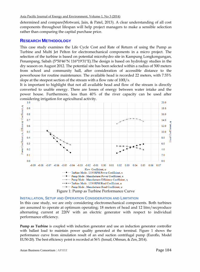
This case study examines the Life Cycle Cost and Rate of Return of using the Pump as Turbine and Multi Jet Pelton for electromechanical components in a micro project. The selection of the turbine is based on potential microhydro site in Kampung Longkongungan, Penampang, Sabah (5°50'46"N 116°19'31"E).The design is based on hydrology studies in the dry season on August 2012. The potential site has been selected within a radius of 500 meters from school and community hall, after consideration of accessible distance to the powerhouse for routine maintenance. The available head is recorded 22 meters, with 7.55% slope at the steepest section of the stream with a flow rate of 100l/s. It is important to highlight that not all available head and flow of the stream is directly converted to usable energy. There are losses of energy between water intake and the power house. Furthermore, less than 40% of the river capacity can be used after considering irrigation for agricultural activity.
Figure 1: Pump as Turbine Performance Curve
INSTALLATION, SETUP AND OPERATION CONSIDERATION AND LIMITATION In this case study, we are only considering electromechanical components. Both turbines are assumed to operate at optimum operating; 18 meters of head and 12 litre/secproduce alternating current at 220V with an electric generator with respect to individual performance efficiency. Pump as Turbine is coupled with induction generator and use an induction generator controller with ballast load to maintain power quality generated at the terminal. Figure 1 shows the performance curve from simulation result of an end suction centrifugal pump (Euroflo, Model EU50-20). The best efficiency point is recorded at 56% (Ismail, Othman, & Zen, 2014).
Asia Pacific Journal of Energy and Environment, Volume 1, No 3 (2014)
Asian Business Consortium | APJEE Page 185
Multi Jet Pelton Turbine is direct coupled to Permanent Magnet Alternator (PMA) with built in voltage regulator. The system generates good power quality and require minimum technical know-how skill to operate, suitable for remote areas. Due to no local microhydro manufacturer, the Multi Jet Pelton Turbine will be purchased from international supplier.
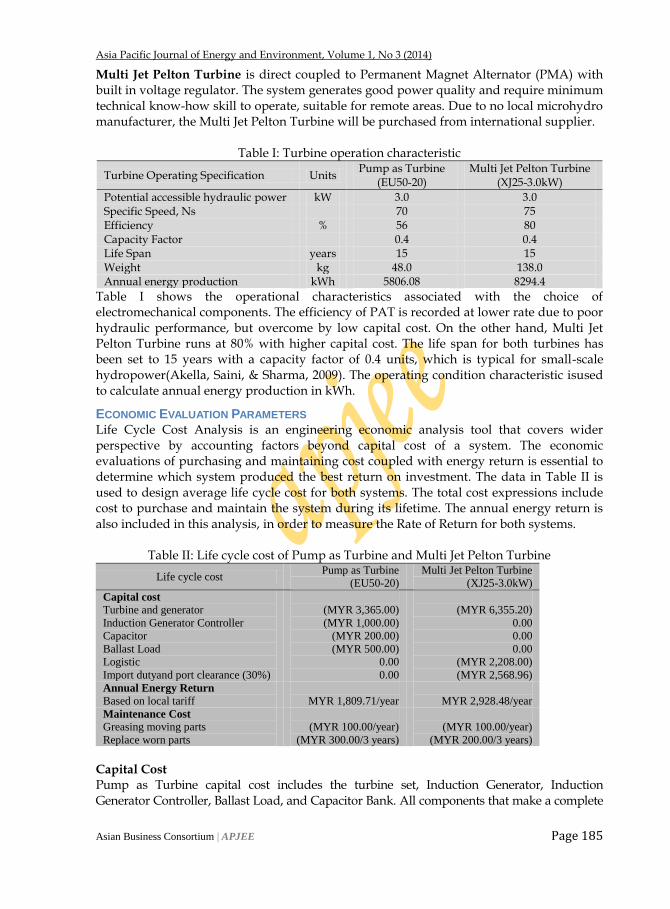
Table I: Turbine operation characteristic
Turbine Operating Specification Units Pump as Turbine
(EU50-20) Multi Jet Pelton Turbine
(XJ25-3.0kW)
Potential accessible hydraulic power kW 3.0 3.0 Specific Speed, Ns 70 75 Efficiency % 56 80 Capacity Factor 0.4 0.4 Life Span years 15 15 Weight kg 48.0 138.0 Annual energy production kWh 5806.08 8294.4
Table I shows the operational characteristics associated with the choice of electromechanical components. The efficiency of PAT is recorded at lower rate due to poor hydraulic performance, but overcome by low capital cost. On the other hand, Multi Jet Pelton Turbine runs at 80% with higher capital cost. The life span for both turbines has been set to 15 years with a capacity factor of 0.4 units, which is typical for small-scale hydropower(Akella, Saini, & Sharma, 2009). The operating condition characteristic isused to calculate annual energy production in kWh.
ECONOMIC EVALUATION PARAMETERS Life Cycle Cost Analysis is an engineering economic analysis tool that covers wider perspective by accounting factors beyond capital cost of a system. The economic evaluations of purchasing and maintaining cost coupled with energy return is essential to determine which system produced the best return on investment. The data in Table II is used to design average life cycle cost for both systems. The total cost expressions include cost to purchase and maintain the system during its lifetime. The annual energy return is also included in this analysis, in order to measure the Rate of Return for both systems.
Table II: Life cycle cost of Pump as Turbine and Multi Jet Pelton Turbine
Life cycle cost Pump as Turbine
(EU50-20)
Multi Jet Pelton Turbine
(XJ25-3.0kW)
Capital cost
Turbine and generator
Induction Generator Controller
Capacitor
Ballast Load
Logistic
Import dutyand port clearance (30%)
(MYR 3,365.00)
(MYR 1,000.00)
(MYR 200.00)
(MYR 500.00)
0.00
0.00
(MYR 6,355.20)
0.00
0.00
0.00
(MYR 2,208.00)
(MYR 2,568.96)
Annual Energy Return
Based on local tariff
MYR 1,809.71/year
MYR 2,928.48/year
Maintenance Cost
Greasing moving parts
Replace worn parts
(MYR 100.00/year)
(MYR 300.00/3 years)
(MYR 100.00/year)
(MYR 200.00/3 years)
Capital Cost Pump as Turbine capital cost includes the turbine set, Induction Generator, Induction Generator Controller, Ballast Load, and Capacitor Bank. All components that make a complete
Asia Pacific Journal of Energy and Environment, Volume 1, No 3 (2014)
Asian Business Consortium | APJEE Page 186
turbine system are purchased locally, therefore excluding the cost of freight and import duty. The Multi Jet Pelton Wheel is purchased from international suppliers. The capital cost acquiring a complete turbine system includes freight charges at the rate of MYR16.00/kg. On top of that, the import duty and port clearance are charge at the rate of 30%. Maintenance Cost Maintenance and repair cost covers consumable items relevant to preventive maintenance and repair of the electromechanical system. The preventive maintenance includes both routine housekeeping and lubricating moving parts, such as bearings, which in turn maintain optimum operating performance and extend lifespan. The scheduled maintenance includes replacing worn parts such as nozzle, impeller and bearings. In terms of repair, replacing parts is carried out based on operation and maintenance manuals for both systems. Energy Revenue
The energy return on the installed systems is measured by converting it to revenue in term of MYR (Malaysia Ringgit) based on Sabah Electric Sdn. Bhd. (SESB) domestic tariff rate. It is important to mention that electricity power in Sabah is partly subsidized by the government, which has a low power tariff among Asia-Pacific countries Present Value (PV) Present value illustrates practical analysis when using currency to measure future cash flow. The calculation using Present Value is appropriate because the analysis considers an investment projection of 15 years life span. For this case study, the discounted rate is set at 5% per annum.
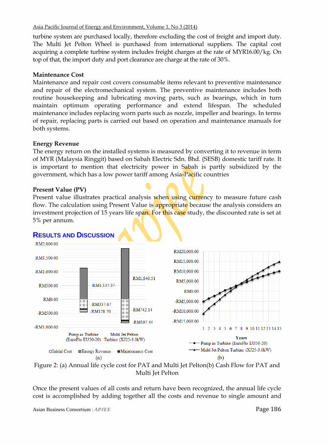
RESULTS AND DISCUSSION
Figure 2: (a) Annual life cycle cost for PAT and Multi Jet Pelton(b) Cash Flow for PAT and
Multi Jet Pelton
Once the present values of all costs and return have been recognized, the annual life cycle cost is accomplished by adding together all the costs and revenue to single amount and
Asia Pacific Journal of Energy and Environment, Volume 1, No 3 (2014)
Asian Business Consortium | APJEE Page 187
divided by the number of life span. The annual life cycle cost of both choices as an electromechanical component in microhydro systems are shown in Figure 2 (a). The total annual net revenue for Pump as Turbine and Multi Jet Pelton Turbine has been recorded at MYR671.00 and MYR990.93, respectively. The annual capital cost for Multi Jet Pelton is significantly higher than Pump as Turbine. The reason of this is from surplus purchasing cost imposed such as freight charges, import duty and port clearance explained earlier in this paper. The annual maintenance cost between both systems is recorded at MYR128.70 and MYR107.44. The Multi Jet Pelton generatesa higher energy return annually since it has higher efficiency. The cash flow of the Pump as Turbine and Multi Jet Pelton Turbine is shown in Figure 2 (b). The Rate of Return for Pump as Turbine and Multi Jet Pelton Turbine is recorded at 4.34 years and 6.11 years respectively. The Pump as Turbine has lower Rate of Return, however lower cumulative profit at MYR 10,065.11 after 15 years. On the other hand, Multi Jet Pelton turbine has longer Rate of Return, but the cumulative profit has been recorded at MYR 14,863.82 with higher return of investment.
CONCLUSION
This case study is intended to show an economic evaluation as one of decision tools to help project managers to choose most economical choices between two or more options. With that in mind, economic evaluations consisting of Life Cycle Cost Analysis and Rate of Return for electromechanical components for Kampung Longkongungan, Sabah, were analysed and compared. All relevant costsoverthe electromechanical operation life span were grouped in three distinct elements, namely capital cost, maintenance cost and energy revenue. The result shows that Pump as Turbine has a low capital cost and shorter Rate of Return. However, due to low efficiency, thetotal return of investment is lower than Multi Jet Pelton Turbine. It is worth to mention that, high capital investment is always an overriding issue for a small community project. However, if there is adequate funding, Multi Jet Pelton Turbine is the best choice forelectromechanical components.
ACKNOWLEDGEMENT
This research was supported by the Centre of Excellence for Renewable Energy (CoERE), Universiti Malaysia Sarawak (UNIMAS) under Grant no. UNIMAS/CoERE/2014/Grant (01).
REFERENCE
Akella, A. K., Saini, R. P., & Sharma, M. P. (2009). Social, Economical and Environmental Impacts of Renewable Energy Systems. Renewable Energy, 34(2), 390-396.
Alexander, K. V., & Giddens, E. P. (2008). Microhydro: Cost-effective, modular systems for low heads. Renewable Energy, 33(6), 1379-1391. doi: 10.1016/j.renene.2007.06.026
Anyi, Martin, Kirke, Brian, & Ali, Sam. (2010). Remote Community Electrification in Sarawak, Malaysia. Renewable Energy, 35(7), 1609-1613.
Arriaga, Mariano. (2010). Pump as Turbine – A Pico-Hydro Alternative in Lao People's Democratic Republic. Renewable Energy, 35(5), 1109-1115.
ASEAN Guideline on Off-grid Rural Electrification Approaches. (2013). In A. C. f. Energy (Ed.). Ismail, Mohd Azlan, Othman, Al Khalid, & Zen, Hushairi. (2014). Numerical Simulation on End Suction
Centrifugal Pump Running in Inverse Flow for Microhydro Applications. Paper presented at the International Integrated Engineering Summit Malaysia.
Kennas, Smail, & Barnett, Andrew. (2000). Best Practices for Sustainable Development of Micro Hydro Power in Developing Countries.

Asia Pacific Journal of Energy and Environment, Volume 1, No 3 (2014)
Asian Business Consortium | APJEE Page 188
McNish, Tyler, Kammen, Daniel M., & Gutierrez, Benjamin. (2010). Clean Energy Options for Sabah: An Analysis of Resource Availability and Cost.
Mishra, Sachin, Singal, S. K., & Khatod, D. K. (2011). Optimal Installation of Small Hydropower Plant—A Review. Renewable and Sustainable Energy Reviews, 15(8), 3862-3869.
Motwani, K. H., Jain, S. V., & Patel, R. N. (2013). Cost Analysis of Pump as Turbine for Pico Hydropower Plants – A Case Study. Procedia Engineering, 51, 721-726.
Murni, S, Whale, J, Davis, JK, Urmee, T, & Harries, D. (2010). Status of Rural Electrification in The ‗Heart of Borneo‘: Role of Micro Hydro Projects.
Murni, Sari, Whale, Jonathan, Urmee, Tania, Davis, John, & Harries, David. (2012). The Role of Micro Hydro Power Systems in Remote Rural Electrification: A Case Study in The Bawan Valley, Borneo. Procedia Engineering, 49(0), 189-196.
Uhunmwangho, R., & Okedu, E.K. (2009). Small Hydropower for Sustainable Development. Pacific Journal of Science and Technology, 10(2), 535-543.
Vaidya, Dr. Cost and Revenue Structures for Micro-Hydro Projects in Nepal. http://www.microhydropower.net/download/mhpcosts.pdf
--0--

Asia Pacific Journal of Energy and Environment, Volume 1, No 3 (2014)
Asian Business Consortium | APJEE Page 189
Wind Power potential in Kigali and Western
provinces of Rwanda
Otieno Fredrick Onyango1, Sibomana Gaston
2, Elie Kabende
3, Felix Nkunda
4,
Jared Hera Ndeda5
1Senior Lecturer, Department of Mathematics and Physical Sciences, Maasai Mara University, Kenya 2,3,4Department of Applied Physics, Kigali Institute of Science and Technology, Rwanda 5Senior Lecturer, Department of Physics, Jomo Kenyatta University of Agriculture & Technology, Kenya
ABSTRACT
Wind speed and wind direction are the most important characteristics for assessing wind energy potential of a location using suitable probability density functions. In this investigation, a hybrid-Weibull probability density function was used to analyze data from Kigali, Gisenyi, and Kamembe stations. Kigali is located in the Eastern side of Rwanda while Gisenyi and Kamembe are to the West. On-site hourly wind speed and wind direction data for the year 2007 were analyzed using Matlab programmes. The annual mean wind speed for Kigali, Gisenyi, and Kamembe sites were determined as 2.36m/s, 2.95m/s and 2.97m/s respectively, while corresponding dominant wind directions for the stations were 3200, 1800 and 1500 respectively. The annual wind power density of Kigali was found to be 13.7W/m2, while the power densities for Gisenyi and Kamembe were determined as 18.4W/m2and 24.4W/m2. It is clear, the investigated regions are dominated by low wind speeds thus are suitable for small-scale wind power generation especially at Kamembe site.
Keywords: Probability density function, Wind power density, Wind speed
INTRODUCTION
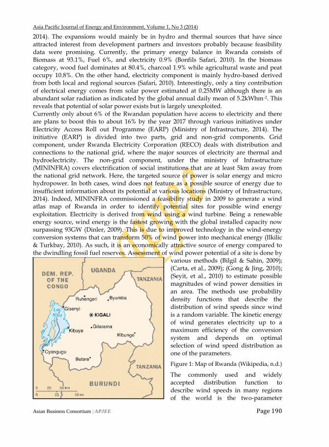
Rwanda is a landlocked country in central Africa with a surface area of 26,338 km2 and located between 20: 00 Latitude South and 300:00 Longitude East. It borders Tanzania to the east, Democratic republic of Congo to the West, Uganda to the North and Burundi to the South (figure 1). Energy supply in the country is mainly from hydro and thermal sources where the former accounts for 26.74MW and the latter contributes 29.57MW against a skyrocketing national demand. Available electricity is therefore insufficient to meet both domestic and industrial needs required for sustainable economic development. The demand for electricity, that continues to rise every year, has necessitated a projected expansion from the current 69MW to 130MW by the year 2015 (Ministry of Infrastructure,
This article is is licensed under a Creative Commons Attribution-NonCommercial 4.0 International License. Attribution-NonCommercial (CC BY-NC) license lets others remix, tweak, and build upon work non-commercially, and although the new works must also acknowledge & be non-commercial.
How to Cite: Onyango OF, Gaston S, Kabende E, Nkunda F, Ndeda JH. Wind Power potential in Kigali and Western provinces of Rwanda Asia Pacific Journal of Energy and Environment. 2014;1(3):189-199.
Source of Support: SFAR Conflict of Interest: Non Declared
DOI prefix 10.15590/apjee
Asia Pacific Journal of Energy and Environment, Volume 1, No 3 (2014)
Asian Business Consortium | APJEE Page 190
2014). The expansions would mainly be in hydro and thermal sources that have since attracted interest from development partners and investors probably because feasibility data were promising. Currently, the primary energy balance in Rwanda consists of Biomass at 93.1%, Fuel 6%, and electricity 0.9% (Bonfils Safari, 2010). In the biomass category, wood fuel dominates at 80.4%, charcoal 1.9% while agricultural waste and peat occupy 10.8%. On the other hand, electricity component is mainly hydro-based derived from both local and regional sources (Safari, 2010). Interestingly, only a tiny contribution of electrical energy comes from solar power estimated at 0.25MW although there is an abundant solar radiation as indicated by the global annual daily mean of 5.2kWhm-2. This reveals that potential of solar power exists but is largely unexploited. Currently only about 6% of the Rwandan population have access to electricity and there are plans to boost this to about 16% by the year 2017 through various initiatives under Electricity Access Roll out Programme (EARP) (Ministry of Infrastructure, 2014). The initiative (EARP) is divided into two parts, grid and non-grid components. Grid component, under Rwanda Electricity Corporation (RECO) deals with distribution and connections to the national grid, where the major sources of electricity are thermal and hydroelectricity. The non-grid component, under the ministry of Infrastructure (MININFRA) covers electrification of social institutions that are at least 5km away from the national grid network. Here, the targeted source of power is solar energy and micro hydropower. In both cases, wind does not feature as a possible source of energy due to insufficient information about its potential at various locations (Ministry of Infrastructure, 2014). Indeed, MININFRA commissioned a feasibility study in 2009 to generate a wind atlas map of Rwanda in order to identify potential sites for possible wind energy exploitation. Electricity is derived from wind using a wind turbine. Being a renewable energy source, wind energy is the fastest growing with the global installed capacity now surpassing 93GW (Dinler, 2009). This is due to improved technology in the wind-energy conversion systems that can transform 50% of wind power into mechanical energy (Ilkilic & Turkbay, 2010). As such, it is an economically attractive source of energy compared to the dwindling fossil fuel reserves. Assessment of wind power potential of a site is done by
various methods (Bilgil & Sahin, 2009); (Carta, et al., 2009); (Gong & Jing, 2010); (Seyit, et al., 2010) to estimate possible magnitudes of wind power densities in an area. The methods use probability density functions that describe the distribution of wind speeds since wind is a random variable. The kinetic energy of wind generates electricity up to a maximum efficiency of the conversion system and depends on optimal selection of wind speed distribution as one of the parameters.
Figure 1: Map of Rwanda (Wikipedia, n.d.)
The commonly used and widely accepted distribution function to describe wind speeds in many regions of the world is the two-parameter

Asia Pacific Journal of Energy and Environment, Volume 1, No 3 (2014)
Asian Business Consortium | APJEE Page 191
Weibull distribution (Himri, et al., 2010). However, it does not represent all wind regimes in every region of the world. In such cases, alternative distributions are required that suit specific wind regimes (Khan & Shahidehpour, 2009).
WIND DATA
The historical wind data used in this study are from Kamembe and Gisenyi stations, both in the Western province of Rwanda, while Kanombe station is in Kigali province. Kamembe is the airport in Cyangugu at the shores of Lake Kivu as shown in figure 1. Meteorological department (Meteo) Rwanda that collects and archives all weather-related information of the country manages the stations. The hourly wind speed and wind direction data were recorded at anemometer height of 10m above ground. Table I gives the measuring year of the data, geographical coordinates, and altitude of the stations. Table I: Geographic parameters of the site
Station latitude Longitude Altitude (m)
Measuring year
Anemometer height(m)
Kamembe 2° 28' 0'' S 28° 55' 0'' E 1491 2007 10
Gisenyi 01° 40' 37.93" S 029°15' 31.95" E 1549 2007 10
Kanombe 1057‘55.33‖S 30008‘05.18‖E 1494 2007 10
MATERIALS AND METHOD
Hybrid-Weibull distribution function
Probability density functions (PDFs) are important in wind studies to estimate the power of a given wind speed which is then compared with the measured probabilities found by getting the ratio of the frequency of a given speed to the total frequency of speeds occurring in a location. The probability density function that has wide appeal as the standard function for wind speed modelling is the Weibull distribution (equation 1), but it is most appropriate for regions with negligible occurrence of null wind speeds. If one cannot ignore the presence of null wind speeds then appropriate modifications to Weibull distribution is necessary. One such modification is the Hybrid Weibull distribution given in equation 2 with ϕ representing the distribution parameters k and c, while θo is the probability of null wind speeds. In this paper, the hybrid Weibull distribution was used for the analysis of wind power density. The hybrid Weibull distribution is well defined (Carta, et al., 2009). Generally, the Weibull probability density function of a random variable v is given in equation 1 where k is a shape parameter while c is a scale parameter. Both of these parameters are functions of mean wind speed and standard deviation as in equation 3 and 4 respectively.
kk
wc
v
c
v
c
kvf exp
1
(1)
Hybrid Weibull distribution ℎ 𝑣,ϕ , 𝜃𝑜 = 𝜃0𝛿 𝑣 + 1 − 𝜃𝑜 𝑓𝑤 (𝑣,ϕ ) (2)
where 𝛿 𝑣 = 1, 𝑖𝑓 𝑣 = 0
0, 𝑖𝑓 𝑣 ≠ 0
𝑘 = 𝜎
𝑣𝑚 −1.086
(1 ≤ 𝑘 ≤ 10) (3)
Asia Pacific Journal of Energy and Environment, Volume 1, No 3 (2014)
Asian Business Consortium | APJEE Page 192
11
mvc
k
(4)
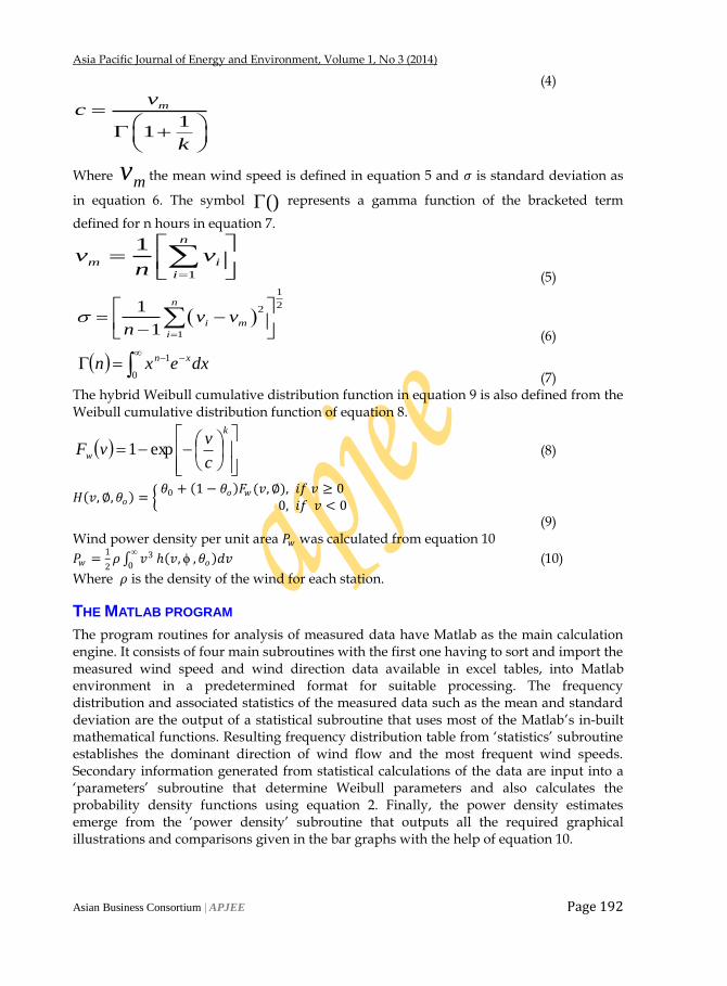
Where mv the mean wind speed is defined in equation 5 and 𝜎 is standard deviation as
in equation 6. The symbol () represents a gamma function of the bracketed term
defined for n hours in equation 7.
1
1 n
m i
i
v vn
(5)
1
22
1
1
1
n
i m
i
v vn
(6)
dxexn xn
0
1
(7) The hybrid Weibull cumulative distribution function in equation 9 is also defined from the Weibull cumulative distribution function of equation 8.
k
wc
vvF exp1 (8)
𝐻 𝑣,∅,𝜃𝑜 = 𝜃0 + 1 − 𝜃𝑜 𝐹𝑤 (𝑣,∅), 𝑖𝑓 𝑣 ≥ 0
0, 𝑖𝑓 𝑣 < 0
(9) Wind power density per unit area 𝑃𝑤 was calculated from equation 10
𝑃𝑤 =1
2𝜌 𝑣3∞
0ℎ 𝑣, ϕ ,𝜃𝑜 𝑑𝑣 (10)
Where 𝜌 is the density of the wind for each station.
THE MATLAB PROGRAM
The program routines for analysis of measured data have Matlab as the main calculation engine. It consists of four main subroutines with the first one having to sort and import the measured wind speed and wind direction data available in excel tables, into Matlab environment in a predetermined format for suitable processing. The frequency distribution and associated statistics of the measured data such as the mean and standard deviation are the output of a statistical subroutine that uses most of the Matlab‘s in-built mathematical functions. Resulting frequency distribution table from ‗statistics‘ subroutine establishes the dominant direction of wind flow and the most frequent wind speeds. Secondary information generated from statistical calculations of the data are input into a ‗parameters‘ subroutine that determine Weibull parameters and also calculates the probability density functions using equation 2. Finally, the power density estimates emerge from the ‗power density‘ subroutine that outputs all the required graphical illustrations and comparisons given in the bar graphs with the help of equation 10.
Asia Pacific Journal of Energy and Environment, Volume 1, No 3 (2014)
Asian Business Consortium | APJEE Page 193
PERFORMANCE ANALYSIS
There are various methods used to analyze convergence between measured data and results that are due to a mathematical model. Performance analysis of results obtained from the Hybrid-Weibull distribution was done using the mean absolute percentage error (MAPE) given in equation 11. The coefficient of correlation between the measured and estimated data was also determined using equation 12.
𝑀𝐴𝑃𝐸 =1
𝑡 𝑎𝑏𝑠
𝑒𝑗−𝑚 𝑗
𝑒𝑗 𝑡
𝑗=1 × 100 (11)
𝑅 =𝑚 .𝑒 −𝑚 .𝑒
𝑚2 −(𝑚 )2 . 𝑒2 −(𝑒 )2
(12)
Where m is the measured wind speed data; e is the estimated data; t is the total number of hours; 𝑒 is the mean of estimated data; 𝑚 is the mean of measured data; 𝑚. 𝑒 is the mean of product of measured and estimated data.
RESULTS AND DISCUSSIONS
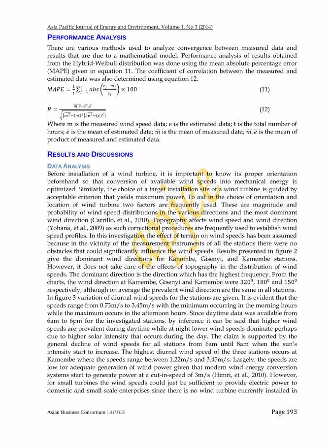
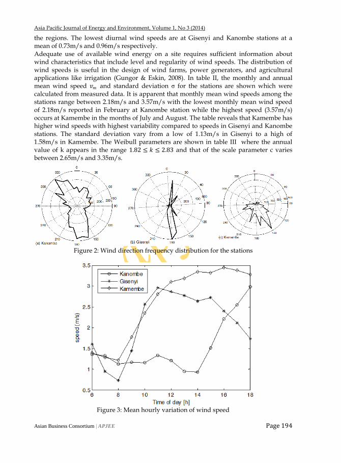
DATA ANALYSIS Before installation of a wind turbine, it is important to know its proper orientation beforehand so that conversion of available wind speeds into mechanical energy is optimized. Similarly, the choice of a target installation site of a wind turbine is guided by acceptable criterion that yields maximum power. To aid in the choice of orientation and location of wind turbine two factors are frequently used. These are magnitude and probability of wind speed distributions in the various directions and the most dominant wind direction (Carrillo, et al., 2010). Topography affects wind speed and wind direction (Yohana, et al., 2009) as such correctional procedures are frequently used to establish wind speed profiles. In this investigation the effect of terrain on wind speeds has been assumed because in the vicinity of the measurement instruments of all the stations there were no obstacles that could significantly influence the wind speeds. Results presented in figure 2 give the dominant wind directions for Kanombe, Gisenyi, and Kamembe stations. However, it does not take care of the effects of topography in the distribution of wind speeds. The dominant direction is the direction which has the highest frequency. From the charts, the wind direction at Kamembe, Gisenyi and Kamembe were 3200, 1800 and 1500 respectively, although on average the prevalent wind direction are the same in all stations. In figure 3 variation of diurnal wind speeds for the stations are given. It is evident that the speeds range from 0.73m/s to 3.45m/s with the minimum occurring in the morning hours while the maximum occurs in the afternoon hours. Since daytime data was available from 6am to 6pm for the investigated stations, by inference it can be said that higher wind speeds are prevalent during daytime while at night lower wind speeds dominate perhaps due to higher solar intensity that occurs during the day. The claim is supported by the general decline of wind speeds for all stations from 6am until 8am when the sun‘s intensity start to increase. The highest diurnal wind speed of the three stations occurs at Kamembe where the speeds range between 1.22m/s and 3.45m/s. Largely, the speeds are low for adequate generation of wind power given that modern wind energy conversion systems start to generate power at a cut-in-speed of 3m/s (Himri, et al., 2010). However, for small turbines the wind speeds could just be sufficient to provide electric power to domestic and small-scale enterprises since there is no wind turbine currently installed in
Asia Pacific Journal of Energy and Environment, Volume 1, No 3 (2014)
Asian Business Consortium | APJEE Page 194
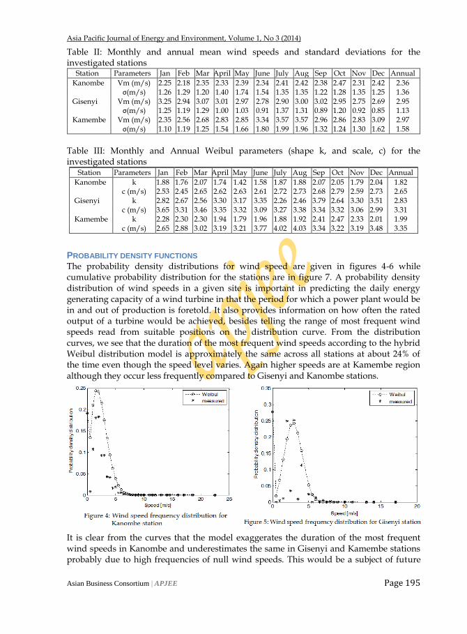
the regions. The lowest diurnal wind speeds are at Gisenyi and Kanombe stations at a mean of 0.73m/s and 0.96m/s respectively. Adequate use of available wind energy on a site requires sufficient information about wind characteristics that include level and regularity of wind speeds. The distribution of wind speeds is useful in the design of wind farms, power generators, and agricultural applications like irrigation (Gungor & Eskin, 2008). In table II, the monthly and annual mean wind speed 𝑣𝑚 and standard deviation σ for the stations are shown which were calculated from measured data. It is apparent that monthly mean wind speeds among the stations range between 2.18m/s and 3.57m/s with the lowest monthly mean wind speed of 2.18m/s reported in February at Kanombe station while the highest speed (3.57m/s) occurs at Kamembe in the months of July and August. The table reveals that Kamembe has higher wind speeds with highest variability compared to speeds in Gisenyi and Kanombe stations. The standard deviation vary from a low of 1.13m/s in Gisenyi to a high of 1.58m/s in Kamembe. The Weibull parameters are shown in table III where the annual value of k appears in the range 1.82 ≤ 𝑘 ≤ 2.83 and that of the scale parameter c varies between 2.65m/s and 3.35m/s.
Figure 2: Wind direction frequency distribution for the stations
Figure 3: Mean hourly variation of wind speed
Asia Pacific Journal of Energy and Environment, Volume 1, No 3 (2014)
Asian Business Consortium | APJEE Page 195
Table II: Monthly and annual mean wind speeds and standard deviations for the investigated stations
Station Parameters Jan Feb Mar April May June July Aug Sep Oct Nov Dec Annual
Kanombe Vm (m/s) 2.25 2.18 2.35 2.33 2.39 2.34 2.41 2.42 2.38 2.47 2.31 2.42 2.36 σ(m/s) 1.26 1.29 1.20 1.40 1.74 1.54 1.35 1.35 1.22 1.28 1.35 1.25 1.36 Gisenyi Vm (m/s) 3.25 2.94 3.07 3.01 2.97 2.78 2.90 3.00 3.02 2.95 2.75 2.69 2.95 σ(m/s) 1.25 1.19 1.29 1.00 1.03 0.91 1.37 1.31 0.89 1.20 0.92 0.85 1.13 Kamembe Vm (m/s) 2.35 2.56 2.68 2.83 2.85 3.34 3.57 3.57 2.96 2.86 2.83 3.09 2.97 σ(m/s) 1.10 1.19 1.25 1.54 1.66 1.80 1.99 1.96 1.32 1.24 1.30 1.62 1.58
Table III: Monthly and Annual Weibul parameters (shape k, and scale, c) for the investigated stations
Station Parameters Jan Feb Mar April May June July Aug Sep Oct Nov Dec Annual
Kanombe k 1.88 1.76 2.07 1.74 1.42 1.58 1.87 1.88 2.07 2.05 1.79 2.04 1.82 c (m/s) 2.53 2.45 2.65 2.62 2.63 2.61 2.72 2.73 2.68 2.79 2.59 2.73 2.65 Gisenyi k 2.82 2.67 2.56 3.30 3.17 3.35 2.26 2.46 3.79 2.64 3.30 3.51 2.83 c (m/s) 3.65 3.31 3.46 3.35 3.32 3.09 3.27 3.38 3.34 3.32 3.06 2.99 3.31 Kamembe k 2.28 2.30 2.30 1.94 1.79 1.96 1.88 1.92 2.41 2.47 2.33 2.01 1.99 c (m/s) 2.65 2.88 3.02 3.19 3.21 3.77 4.02 4.03 3.34 3.22 3.19 3.48 3.35
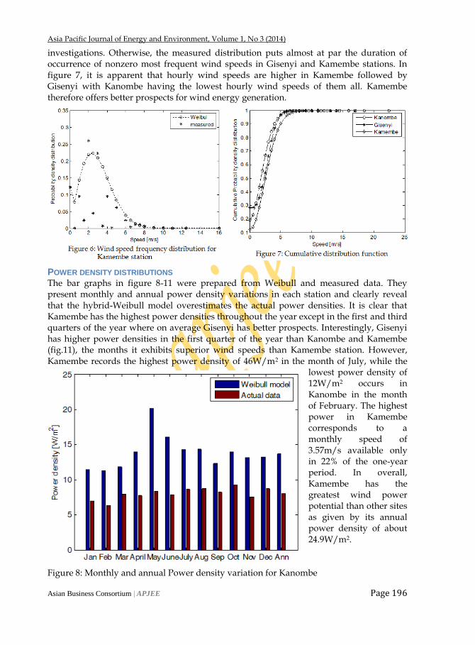
PROBABILITY DENSITY FUNCTIONS The probability density distributions for wind speed are given in figures 4-6 while cumulative probability distribution for the stations are in figure 7. A probability density distribution of wind speeds in a given site is important in predicting the daily energy generating capacity of a wind turbine in that the period for which a power plant would be in and out of production is foretold. It also provides information on how often the rated output of a turbine would be achieved, besides telling the range of most frequent wind speeds read from suitable positions on the distribution curve. From the distribution curves, we see that the duration of the most frequent wind speeds according to the hybrid Weibul distribution model is approximately the same across all stations at about 24% of the time even though the speed level varies. Again higher speeds are at Kamembe region although they occur less frequently compared to Gisenyi and Kanombe stations.
It is clear from the curves that the model exaggerates the duration of the most frequent wind speeds in Kanombe and underestimates the same in Gisenyi and Kamembe stations probably due to high frequencies of null wind speeds. This would be a subject of future
Asia Pacific Journal of Energy and Environment, Volume 1, No 3 (2014)
Asian Business Consortium | APJEE Page 196
investigations. Otherwise, the measured distribution puts almost at par the duration of occurrence of nonzero most frequent wind speeds in Gisenyi and Kamembe stations. In figure 7, it is apparent that hourly wind speeds are higher in Kamembe followed by Gisenyi with Kanombe having the lowest hourly wind speeds of them all. Kamembe therefore offers better prospects for wind energy generation.
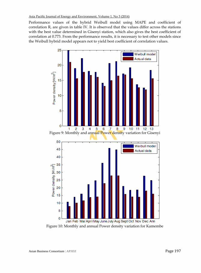
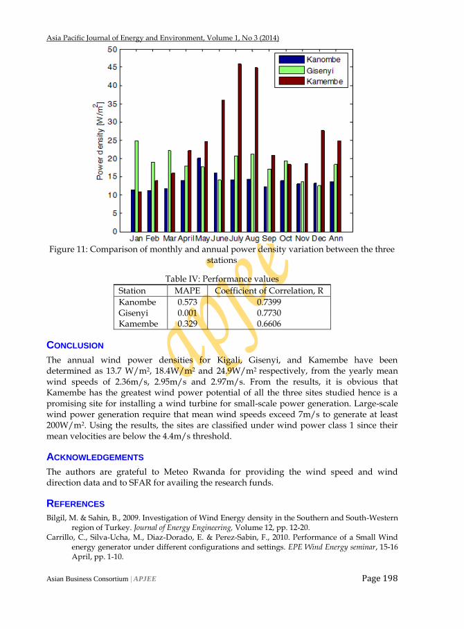
POWER DENSITY DISTRIBUTIONS The bar graphs in figure 8-11 were prepared from Weibull and measured data. They present monthly and annual power density variations in each station and clearly reveal that the hybrid-Weibull model overestimates the actual power densities. It is clear that Kamembe has the highest power densities throughout the year except in the first and third quarters of the year where on average Gisenyi has better prospects. Interestingly, Gisenyi has higher power densities in the first quarter of the year than Kanombe and Kamembe (fig.11), the months it exhibits superior wind speeds than Kamembe station. However, Kamembe records the highest power density of 46W/m2 in the month of July, while the
lowest power density of 12W/m2 occurs in Kanombe in the month of February. The highest power in Kamembe corresponds to a monthly speed of 3.57m/s available only in 22% of the one-year period. In overall, Kamembe has the greatest wind power potential than other sites as given by its annual power density of about 24.9W/m2.
Figure 8: Monthly and annual Power density variation for Kanombe
Asia Pacific Journal of Energy and Environment, Volume 1, No 3 (2014)
Asian Business Consortium | APJEE Page 197
Performance values of the hybrid Weibull model using MAPE and coefficient of correlation R, are given in table IV. It is observed that the values differ across the stations with the best value determined in Gisenyi station, which also gives the best coefficient of correlation at 0.773. From the performance results, it is necessary to test other models since the Weibull hybrid model appears not to yield best coefficient of correlation values.
Figure 9: Monthly and annual Power density variation for Gisenyi
Figure 10: Monthly and annual Power density variation for Kamembe
Asia Pacific Journal of Energy and Environment, Volume 1, No 3 (2014)
Asian Business Consortium | APJEE Page 198
Figure 11: Comparison of monthly and annual power density variation between the three
stations
Table IV: Performance values
Station MAPE Coefficient of Correlation, R
Kanombe 0.573 0.7399 Gisenyi 0.001 0.7730 Kamembe 0.329 0.6606
CONCLUSION
The annual wind power densities for Kigali, Gisenyi, and Kamembe have been determined as 13.7 W/m2, 18.4W/m2 and 24.9W/m2 respectively, from the yearly mean wind speeds of 2.36m/s, 2.95m/s and 2.97m/s. From the results, it is obvious that Kamembe has the greatest wind power potential of all the three sites studied hence is a promising site for installing a wind turbine for small-scale power generation. Large-scale wind power generation require that mean wind speeds exceed 7m/s to generate at least 200W/m2. Using the results, the sites are classified under wind power class 1 since their mean velocities are below the 4.4m/s threshold.
ACKNOWLEDGEMENTS
The authors are grateful to Meteo Rwanda for providing the wind speed and wind direction data and to SFAR for availing the research funds.
REFERENCES
Bilgil, M. & Sahin, B., 2009. Investigation of Wind Energy density in the Southern and South-Western region of Turkey. Journal of Energy Engineering, Volume 12, pp. 12-20.
Carrillo, C., Silva-Ucha, M., Diaz-Dorado, E. & Perez-Sabin, F., 2010. Performance of a Small Wind energy generator under different configurations and settings. EPE Wind Energy seminar, 15-16 April, pp. 1-10.
Asia Pacific Journal of Energy and Environment, Volume 1, No 3 (2014)
Asian Business Consortium | APJEE Page 199
Carta, J. A., Ramirez, P. & Velazquez, S., 2009. A Review of Wind speed probability distributions used in Wind Energy analysi: Case studies in the Canary Islands.. Renewable and Sustainable Energy Reviews, Volume 13, pp. 933-955.
Dinler, S. A. A. a. A., 2009. A new method to estimate Weibull parameters for wind Energy Applications. Energy Conversion and management, Volume 50, pp. 1761-1766.
Gong, L. & Jing, S., 2010. Application of Bayesian model averaging in modelling long-term wind speed distributions. Renewable Energy, Volume 35, pp. 1192-1202.
Gungor, A. & Eskin, N., 2008. The Characteristics that define Wind as an Energy Source. Energy Sources part (A), Volume 30, pp. 842-855.
Himri, Y., Himri, S. & A, B. S., 2010. Wind Speed Data Analysis used in Installation of Wind Energy Conversion Systems in Algeria. New Orleans, LA, USA, IEEE.
Ilkilic, C. & Turkbay, I., 2010. Determination and Utilization of Wind Energy potential for Turkey. Renewable and Sustainable Energy Reviews, Volume 14, pp. 2202-2207.
Islam MA, Bhuiya MA and Islam MS. 2014. A Review on Chemical Synthesis Process of Platinum Nanoparticles Asia Pacific Journal of Energy and Environment, 1, 107-120.
Khan, A. A. & Shahidehpour, M., 2009. Day Ahead Wind Speed Forecasting using Wavelets. Seattle, WA USA, IEEE.
Ministry of Infrastructure, 2011. [Online] Available at: http://mininfra.gov.rw/ [Accessed 20 January 2014].
Safari, B., 2010. A review of Energy in Rwanda. Renewable and Sustainable Energy reviews, Volume 14, pp. 524-529.
Seyit, A. A., Bagiorgas, H. S. & Mihalakakou, G., 2010. Use of two-component Weibull mixtures in the analysis of wind speed in the Eastern mediterranean. Applied Energy, Volume 87, pp. 2566-2573.
Wikipedia, n.d. Rwanda. [Online] Available at: http://en.wikipedia.org/wiki/Rwanda [Accessed 3 August 2014].
Yohana, N. M., Sungsu, L. & Young-Kyu, L., 2009. Topographical Effects on Wind Speed over various terrains: A Case Study for Korean Peninsula. The Seventh Asia-Pacific Conference on Wind Engineering, 8-12 November.

Asia Pacific Journal of Energy and Environment, Volume 1, No 3 (2014)
Asian Business Consortium | APJEE Page 200
Bearings-Only Tracking of Manoeuvring Targets
Using Multiple Model Variable Rate Particle
Filter with Differential Evolution
Ghasem Saeidi, M. R. Moniri
Department of Communication Engineering, Islamic Azad University, Shahr-e-Rey Branch, Iran
ABSTRACT
In standard target tracking, algorithms assume synchronous and identical sampling rate for measurement and state processes. Contrary to these methods particle filter is proposed with variable rate. These filters use a restricted number of states, and a Gamma distribution is applied at state arrival time so that the maneuvering targets could be tracked. Although this structure is capable of tracking a wide range of targets motion features using linear, curvilinear motion dynamics, it suffers from a basic weak point. It cannot estimate the position of targets in high maneuvering regions. Thus, multiple model variable rate particle filter (MM-VRPF) is utilized to overcome this shortage using various dynamic models. A weak point of a particle filter is a phenomenon called degeneracy that even exists in MM-VRPF structure. In this study, differential evolution method, is exploited to improve the mentioned method and a novel structure called multiple model variable rate particle filter with differential evolution (MM-VRPF with DE) is introduced. The simulation results of a bearing only tracking achieved from a maneuvering target, revealed that the proposed structure has better performance while it maintains advantages of variable rate structure.
Key words: Target tracking, Multiple model variable rate particle filter, Differential evolution
INTRODUCTION
General speaking tracking is referred to obtaining kinematic parameters of the target (such as location, velocity, acceleration) during a time interval based on noisy observations. During the last decade tracking maneuvering targets have experienced increasing progress and has attracted great attention owing to the development of numerical techniques (Jilkov, 2003). Estimation in nonlinear systems is a prominent issue in many applications. Bayesian field is one of the most popular estimation techniques. From its perspective, the objective is to estimate a stochastic process based on noisy observations. In this framework state space equations are common. The goal is to estimate the state of a
This article is is licensed under a Creative Commons Attribution-NonCommercial 4.0 International License. Attribution-NonCommercial (CC BY-NC) license lets others remix, tweak, and build upon work non-commercially, and although the new works must also acknowledge & be non-commercial.
How to Cite: Saeidi G, Moniri MR. Bearings-Only Tracking of Manoeuvring Targets Using Multiple Model Variable Rate Particle Filter with Differential Evolution Asia Pacific Journal of Energy and Environment. 2014;1(3):200-214.
Source of Support: Nil Conflict of Interest: Declared
DOI prefix 10.15590/apjee

Asia Pacific Journal of Energy and Environment, Volume 1, No 3 (2014)
Asian Business Consortium | APJEE Page 201
dynamic system based on noisy observations that are a function of system state. In Bayesian filter, it is desired to estimate posterior probability density function. Knowing the probability density, an optimized estimation of states might be achieved, and it could be calculated proportionate to every criterion function. Since this filter does not have a closed solution, different methods have been proposed for its implementation in accordance with process and measurement model. With this regard for limited linear dynamic systems grid, based filters are utilized Fox (2003), Boers (1999). Furthermore in case of a nonlinear system and Gaussian noise Extended Kalman Filter (EKF) is exploited Ristic (2004), Simon (2006). Increase in nonlinearity of the system, the estimation results are distorted, and the posterior probability function violates Gaussian state and destroys the estimations Ristic, (2004), Arulampalam (2002). Another practical solution for implementation of Bayesian filters is using nonparametric methods among that the most important one is the particle filter (Gordon, 1993). In the above-mentioned filter posterior probability density function is estimated by a set consisting of weighted a particles Ristic, (2004), Arulampalam (2002). In standard methods for target tracking and particularly in particle filter, the state sampling rate is determined proportionate to measurement rate. A modern and economic approach is utilizing variable rate particle filter (VRPF) where state arrival times (new states) are modeled as pseudo-Markovian random process. Although this structure would be able to track different features of motion using linear, curvilinear motion dynamic model, it is not capable of providing a precise estimation in regions with high maneuver. To address this problem, a structure with multiple models might be employed that models, target motion dynamics using a set of models and it can switch between these models. The modified structure is called multiple mode variable rate particle filter (MM-VRPF). Using this method continuous certain process proposed in Godsill (2007), Ulker (2012) will be maintained; meanwhile, they would be adapted to variable rate structure with multiple models, so that the tracking operation is improved. The most essential weak point that must be taken into considerations in particle filters is the degeneracy phenomenon that results from an increase in variance of weights (Doucet, 2000). In practice, it has been observed that most of the samples have normalized weight close to zero after a short time, and only one sample has a large weight. So the weights of some samples are calculated whereas they have a negligible effect on the final estimation that is a waste of power. To address this issue resampling is utilized. In resampling stage, weighted samples at the end of a step, are sampled N times. The chance of each sample for being selected depends on its weight. As a result, in this step samples with greater weights are copied several times and samples with smaller weights would be eliminated. At the end of this step a non-weighted estimation of joint posterior distribution is achieved. Numerous algorithms have been proposed for resampling; in (Doucand, 2005) a good comparison is presented. Resampling method improves degeneracy (Gordon, 1993); however, it has a crucial weakness called sample impoverishment. It is due to repeat of samples with large weight. It causes all samples to have the same history after a specific time step. In this paper differential evolution optimization algorithms are utilized to mitigate degeneracy an a new set of filters are introduced; multiple model variable rate particle filter with differential evolution (MM-VRPF with DE). In this algorithm particles are optimized using differential evolution algorithm and they are combined with a random set obtained by probability distribution in variable rate structure, so that better solution is derived. The simulation results illustrated that proposed structure increases efficiency and precision in path estimation compared to MM-VRPF.
Asia Pacific Journal of Energy and Environment, Volume 1, No 3 (2014)
Asian Business Consortium | APJEE Page 202
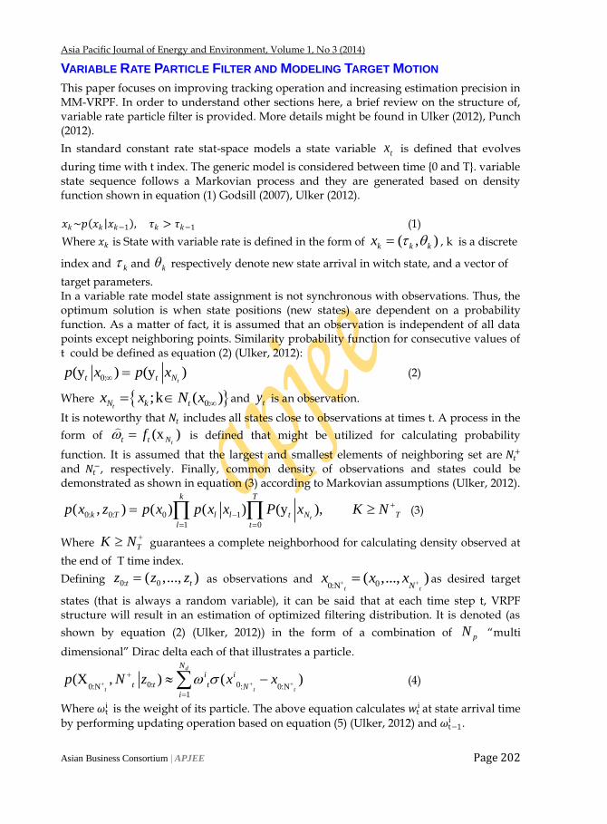
VARIABLE RATE PARTICLE FILTER AND MODELING TARGET MOTION
This paper focuses on improving tracking operation and increasing estimation precision in MM-VRPF. In order to understand other sections here, a brief review on the structure of, variable rate particle filter is provided. More details might be found in Ulker (2012), Punch (2012).
In standard constant rate stat-space models a state variable tx is defined that evolves
during time with t index. The generic model is considered between time {0 and T}. variable state sequence follows a Markovian process and they are generated based on density function shown in equation (1) Godsill (2007), Ulker (2012). 𝑥𝑘~𝑝 𝑥𝑘 𝑥𝑘−1 , 𝜏𝑘 > 𝜏𝑘−1 (1)
Where 𝑥𝑘 is State with variable rate is defined in the form of ( , )k k kx , k is a discrete
index and k and k respectively denote new state arrival in witch state, and a vector of
target parameters. In a variable rate model state assignment is not synchronous with observations. Thus, the optimum solution is when state positions (new states) are dependent on a probability function. As a matter of fact, it is assumed that an observation is independent of all data points except neighboring points. Similarity probability function for consecutive values of t could be defined as equation (2) (Ulker, 2012):
0:(y ) (y )tt t Np x p x (2)
Where 0:;k ( )tN k tx x N x and ty is an observation.
It is noteworthy that 𝑁𝑡 includes all states close to observations at times t. A process in the
form of (x )tt t Nf
is defined that might be utilized for calculating probability
function. It is assumed that the largest and smallest elements of neighboring set are 𝑁𝑡+
and 𝑁𝑡−, respectively. Finally, common density of observations and states could be
demonstrated as shown in equation (3) according to Markovian assumptions (Ulker, 2012).
0: 0: 0 1
1 0
( , ) ( ) ( ) (y ),t
k T
k T l l t N T
l t
p x z p x p x x P x K N
(3)
Where TK N guarantees a complete neighborhood for calculating density observed at
the end of T time index.
Defining 0: 0( ,..., )t tz z z
as observations and 00:N( ,..., )
t tNx x x as desired target
states (that is always a random variable), it can be said that at each time step t, VRPF structure will result in an estimation of optimized filtering distribution. It is denoted (as
shown by equation (2) (Ulker, 2012)) in the form of a combination of pN ―multi
dimensional‖ Dirac delta each of that illustrates a particle.
0: 00:N : 0:N1
(X , ) ( )d
t t t
Ni i
t t t Ni
p N z x x
(4)
Where 𝜔ti
is the weight of its particle. The above equation calculates 𝑤t
i at state arrival time
by performing updating operation based on equation (5) (Ulker, 2012) and 𝜔t−1i .
Asia Pacific Journal of Energy and Environment, Volume 1, No 3 (2014)
Asian Business Consortium | APJEE Page 203
1 1
1 1
1:N
1
0:1:N
( ) ( )
( , )
t t t t
t t t
i i i
t N N Ni i
t ti i
tN N
p y x p x x
q x x y
(5)
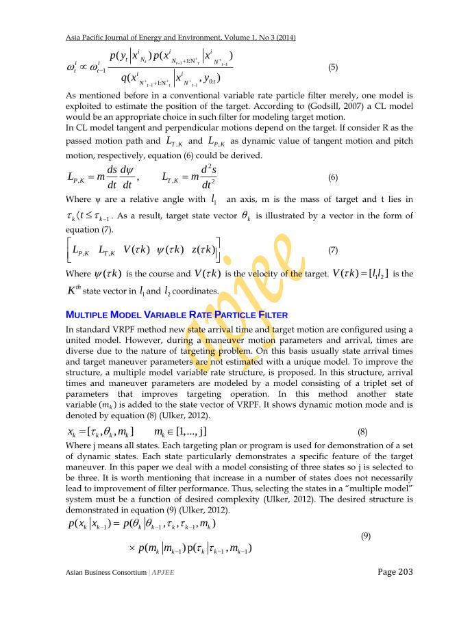
As mentioned before in a conventional variable rate particle filter merely, one model is exploited to estimate the position of the target. According to (Godsill, 2007) a CL model would be an appropriate choice in such filter for modeling target motion. In CL model tangent and perpendicular motions depend on the target. If consider R as the
passed motion path and ,T KL and ,P KL as dynamic value of tangent motion and pitch
motion, respectively, equation (6) could be derived. 2
, , 2,P K T K
ds d d sL m L m
dt dt dt
(6)
Where ψ are a relative angle with 1l an axis, m is the mass of target and t lies in
1k kt . As a result, target state vector k is illustrated by a vector in the form of
equation (7).
, , ( ) ( ) ( )P K T KL L V k k z k
(7)
Where ( )k is the course and ( )V k is the velocity of the target. 1 2( ) [ ]V k l l is the
thK state vector in 1l and 2l coordinates.
MULTIPLE MODEL VARIABLE RATE PARTICLE FILTER
In standard VRPF method new state arrival time and target motion are configured using a united model. However, during a maneuver motion parameters and arrival, times are diverse due to the nature of targeting problem. On this basis usually state arrival times and target maneuver parameters are not estimated with a unique model. To improve the structure, a multiple model variable rate structure, is proposed. In this structure, arrival times and maneuver parameters are modeled by a model consisting of a triplet set of parameters that improves targeting operation. In this method another state variable 𝑚𝑘 is added to the state vector of VRPF. It shows dynamic motion mode and is denoted by equation (8) (Ulker, 2012).
[ , , ] [1,..., j]k k k k kx m m (8)
Where j means all states. Each targeting plan or program is used for demonstration of a set of dynamic states. Each state particularly demonstrates a specific feature of the target maneuver. In this paper we deal with a model consisting of three states so j is selected to be three. It is worth mentioning that increase in a number of states does not necessarily lead to improvement of filter performance. Thus, selecting the states in a ―multiple model‖ system must be a function of desired complexity (Ulker, 2012). The desired structure is demonstrated in equation (9) (Ulker, 2012).
1 1 1
1 1 1
( ) ( , , , )
( ) p( , )
k k k k k k k
k k k k k
p x x p m
p m m m
(9)
Asia Pacific Journal of Energy and Environment, Volume 1, No 3 (2014)
Asian Business Consortium | APJEE Page 204
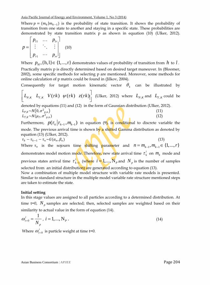
Where 𝑝 = (𝑚𝑘 𝑚𝑘−1) is the probability of state transition. It shows the probability of
transition from one state to another and staying in a specific state. These probabilities are demonstrated by state transition matrix p as shown in equation (10) (Ulker, 2012).
11 1
1
r
r rr
p p
p
p p
(10)
Where ,{h, l} {1,..., r}hlp demonstrates values of probability of transition from h to l .
Practically matrix p is directly determined based on desired target maneuver. In (Bloomer, 2002), some specific methods for selecting p are mentioned. Moreover, some methods for online calculation of p matrix could be found in (Jilkov, 2004).
Consequently for target motion kinematic vector k can be illustrated by
, , ( ) ( ) ( )P K T KL L V k k z k
(Ulker, 2012) where ,P KL and ,T KL could be
denoted by equations (11) and (12) in the form of Gaussian distribution (Ulker, 2012).
𝐿𝑃,𝐾~𝑁 0,𝜎2𝑝 ,𝑛 (11)
𝐿𝑇,𝐾~𝑁(𝜇𝑇 ,𝜎2𝑝 ,𝑛) (12)
Furthermore, 1 1( , )k k kp m
in equation (9), is conditional to discrete variable the
mode. The previous arrival time is shown by a shifted Gamma distribution as denoted by equation (13) (Ulker, 2012). 𝜏𝑘 − 𝜏𝑘−1 − 𝜏𝑛~𝐺(𝛼𝑛 ,𝛽𝑛) (13)
Where 𝜏𝑛 is the sojourn time shifting parameter and 1 1, {1,..., }k kn m m r
demonstrates model motion mode. Therefore, new state arrival time i
k on km
mode and
previous states arrival time i
k 1 (where 1,..., NPi and pN is the number of samples
selected from an initial distribution) are generated according to equation (13). Now a combination of multiple model structure with variable rate models is presented. Similar to standard structure in the multiple model variable rate structure mentioned steps are taken to estimate the state.
Initial setting In this stage values are assigned to all particles according to a determined distribution. At
time t=0, pN samples are selected; then, selected samples are weighted based on their
similarity to actual value in the form of equation (14).
0
1i
t
pN , 1,..., N .Pi (14)
Where 0
i
t is particle weight at time t=0.
Asia Pacific Journal of Energy and Environment, Volume 1, No 3 (2014)
Asian Business Consortium | APJEE Page 205
Propagation step
In this step as soon as a new state arrives, pN samples are selected based on q(.)
distribution that plays the role of previous state distribution. q(.) distribution is stated as shown by equation (15) (Ulker, 2012).
1 1 1 1:1:N 1:
( , ) ( )t t t t t t
i i
o tN N N N Nq x x y p x x
(15)
Updating the particle weights
Updating is performed based on a simplified form of equation (5). In this equation if previous distribution q(.) is utilized, a simpler equation in the form of equation (16) is
derived (Ulker, 2012) that is exploited for calculating particle weights , 1,..., Ni
t Pi .
1 ( )t
i i i
t t t Np y x (16)
Thus, ( )t
i
t Np y x probability in updating operation of i
t could be defined in the form of
equation (17).
( ) ( )tt N t tp y x p y
(17)
Finally, it could be concluded that posterior probability function 0:( , | )t t tp x y
N N is
estimated by associated weight vectors {𝑦𝑡𝑖}
𝑖=1
𝑁𝑝 and particles {𝑥𝒩𝑡
𝑖 }𝑖=1
𝑁𝑝. Afterwards, if
2
1
1
( )p
eff N
i
t
i
N
w
is less than default threshold value, resampling operation will be done.
MM-VRPF structure does not need regeneration stage whereas it is necessary for VRPF framework; thus, it considerably reduces a computational load (Ulker, 2012).
DIFFERENTIAL EVOLUTION
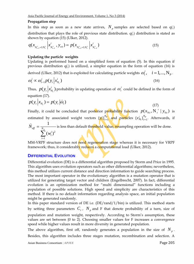
Differential evolution (DE) is a differential algorithm proposed by Storm and Price in 1995. This algorithm uses evolution operators such as other differential algorithms; nevertheless, this method utilizes current distance and direction information to guide searching process. The most important operator in the evolutionary algorithm is a mutation operator that is utilized for generating target vector and children (Engelbrecht, 2007). In fact, differential evolution is an optimization method for ―multi dimensional‖ functions including a population of possible solutions. High speed and simplicity are characteristics of this method. If there is no default information regarding analysis space, an initial population might be generated randomly. In this paper standard version of DE i.e. (DE/rand/1/bin) is utilized. This method starts
by setting three parameters rC , pN and F that denote probability of a turn, size of
population and mutation weight, respectively. According to Storm‘s assumption, these values are set between {0 to 2}. Choosing smaller values for F increases a convergence speed while higher values result in more diversity in generated population.
The above algorithm, first off, randomly generates a population in the size of pN .
Besides, this algorithm includes three stages mutation, recombination and selection. A

Asia Pacific Journal of Energy and Environment, Volume 1, No 3 (2014)
Asian Business Consortium | APJEE Page 206
population in the form of i
Gp is considered and a vector whose length is pN . The vector
includes elements in the form of J,G
ip illustrating the size of a population where j is the
position in R-dimension unique element and G demonstrates the generation to that the
population belongs. i is an index for each element in i
Gp ; these triple steps are briefly
explained Engelbrecht (2007), Rahnamayan (2008), Das (2005).
Mutation In this stage, three vectors are randomly selected so that they are mutually different. The result is a directed vector that is shown in the form of equation (18) for each vector inside the population.
31 2 ( )( ) ( )( ) *( )rr ri
j j j jx p F p p (18)
Where 1,..., pi N and, 1r , 2r and 3r
are mutually different random vectors that are
selected based on {1,..., }pN .
Recombination
In this stage mutated vector components are transferred to candidate vector with equal
probability of rC ; otherwise, equivalent component will be substituted in main vector and
shown in the form of equation (19).
,( )
,
,
( ) ()i
j G ri
j G
i
j G
x if rand j c or j randbu
p else
(19)
Where rand(j) demonstrates a jth call of a random function that is a number between {0 and 1}. To make sure that at least one component is transferred to test vector, one component is
transferred from the mutated vector to test vector disregarding rC . So, for each candidate
vector one component is selected for transferring to a next generation.
Selection To select residuals, each vector is compared to corresponding candidate vector. As a result, each of them that is more competent will be transferred to the next generation.
By selecting vector 𝑥𝐺(𝑖)
or 𝑃𝐺(𝑖)
as a member of next generation 1G , one may write
according to equation (20).
( ) ( ) ( )( )
1( )
, ( ) (x )i i ii G G G
Gi
G
x if f p fp
p else
(20)
In the algorithm (1) DE performance would be introduced as a pseudocode. ............................................................................................................................. ........ Algorithm 1. D E ............................................................................................................................. .......
Input: Initialize and evaluate population pN

Asia Pacific Journal of Energy and Environment, Volume 1, No 3 (2014)
Asian Business Consortium | APJEE Page 207
Repeat
For 1 pi N do
Select 1( )rp to 3( )r
p , where 1 2 3r r r i
// Selecting R, as the dimension of a particle
( (0,1))randj floor R rand
For 1,...,j R do
if (0,1) r randrand C or j j then
31 2 ( )( ) ( )( ) *( )
rr ri
j j j jx p F p p
else
( ) ( )i i
j jx p
end if end for end for // select next generation
for 1 pi N do
If ( ) ( )( ) (x )i if p f then
( ) ( )i ip x
end if end for Termination conditions ………………………………………………………………………………………
MULTIPLE MODEL VARIABLE RATE PARTICLE FILTER WITH DIFFERENTIAL EVOLUTION
Degeneracy phenomenon is a weakness of the particle filter. This phenomenon is resulted from variance of sample weights, and it is still a problem in MM-VRPF structure. Many efforts have been made to generate a new group of particles that can generate higher weights such that these particles are substituted for particles with much smaller weights. In this paper, differential evolution algorithm is exploited to obtain such particles. These particles have the most proper unique values. With this regard, the fitness function in DE is a function for calculating the weight of a particle. In the algorithm (2) the result of merging DE and MM-VRPF algorithm is presented. Lines starting by (///) demonstrate changes that are resulted after merging. ................................................................................................. ........................................ Algorithm 2. MM-VRPF with DE ............................................................................................................................. ............... Input: Initialization
Set t = 0
For 1 pi N , draw equally weighted samples, 𝑥0𝑖 ~𝑝(𝑥0) from the predefined.
Asia Pacific Journal of Energy and Environment, Volume 1, No 3 (2014)
Asian Business Consortium | APJEE Page 208
Initial step /// distribution and set t = 1 with optimal states that are calculated by differential
Evolution.
Propagation step
Set 𝑘 = 𝑁 + 𝑡 − 1
for 1 pi N
- during the neighborhood i
tN are incomplete
* Set k = k + 1 and draw samples form the proposal distribution
𝑥𝑘𝑖 ~𝑞(𝑥𝑘 𝑥𝑘−1, 𝑦𝑡) until .k t
/// The particles are optimized by differential evolution. /// Mixing particles that is achieved from two pervious steps with the parameter 𝑁𝑑 .
Weight update step Calculate the particle weights
1 1
1 1
1:N
1
0:1:N
( ) ( )
( , )
t t t t
t t t
i i i
t N N Ni i
t ti i
tN N
p y x p x xw w
q x x y
Normalize the particle weights.
Resampling step
Resample xNt
i , wti
i=1
NP if effective sample size N eff =
1
(w ti )2Np
i=1
, is Below a
preset a threshold. Set 𝑡 = 𝑡 + 1.
Iterate through Propagation step
..........…………………………………………………………………………………………
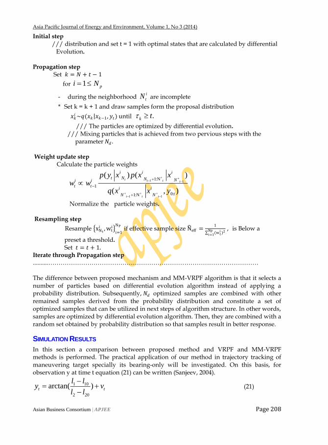
The difference between proposed mechanism and MM-VRPF algorithm is that it selects a number of particles based on differential evolution algorithm instead of applying a probability distribution. Subsequently, 𝑁𝑑 optimized samples are combined with other remained samples derived from the probability distribution and constitute a set of optimized samples that can be utilized in next steps of algorithm structure. In other words, samples are optimized by differential evolution algorithm. Then, they are combined with a random set obtained by probability distribution so that samples result in better response.
SIMULATION RESULTS
In this section a comparison between proposed method and VRPF and MM-VRPF methods is performed. The practical application of our method in trajectory tracking of maneuvering target specially its bearing-only will be investigated. On this basis, for observation y at time t equation (21) can be written (Sanjeev, 2004).
1 10
2 20
arctan( )t t
l ly v
l l
(21)
Asia Pacific Journal of Energy and Environment, Volume 1, No 3 (2014)
Asian Business Consortium | APJEE Page 209
Where arctan(.) demonstrates nonlinear relationship, vt~N(0,σθ2) is the sensor noise and
10 20
Tl l denotes the position of sensor (Sanjeev, 2004).
There are two efficiency measures for evaluation of tracking filters; time averaged root mean
square position error ( )RMSE
and instant root mean square position error(RMSE)t are
mentioned in equation (22). The achieved values for these two measures are obtained by Monte Carlo method with L=100 runs (Ulker, 2012).
2
2
2 2
1 1 2
1
2 2
1 1 2
1 1
1( ) ( )
1( ) ( )
Li i i i
t t t t t
i
T Li i i i
t t t t
t i
RMSE l l l lT
RMSE l l l lLT
(22)
Where T is an index to the last observation. Moreover, for executing it run i
tl
and i
tl
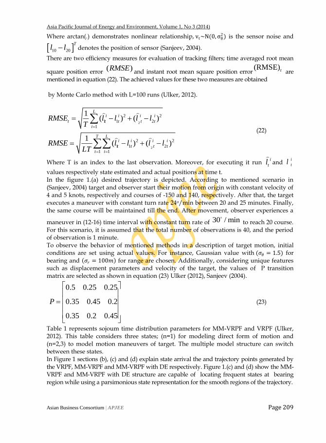
values respectively state estimated and actual positions at time t. In the figure 1.(a) desired trajectory is depicted. According to mentioned scenario in (Sanjeev, 2004) target and observer start their motion from origin with constant velocity of 4 and 5 knots, respectively and courses of -150 and 140, respectively. After that, the target executes a maneuver with constant turn rate 24o/min between 20 and 25 minutes. Finally, the same course will be maintained till the end. After movement, observer experiences a
maneuver in (12-16) time interval with constant turn rate of 30 / min to reach 20 course.
For this scenario, it is assumed that the total number of observations is 40, and the period of observation is 1 minute. To observe the behavior of mentioned methods in a description of target motion, initial conditions are set using actual values. For instance, Gaussian value with (𝜎𝜃 = 1.5) for bearing and 𝜎𝑟 = 100𝑚
for range are chosen. Additionally, considering unique features
such as displacement parameters and velocity of the target, the values of P transition matrix are selected as shown in equation (23) Ulker (2012), Sanjeev (2004).
0.5 0.25 0.25
0.35 0.45 0.2
0.35 0.2 0.45
P
(23)
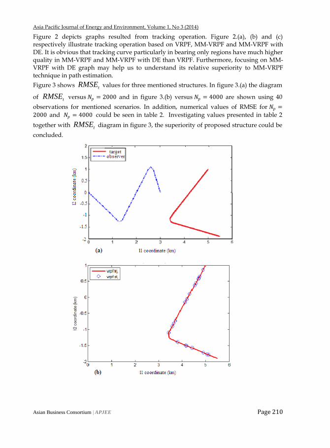
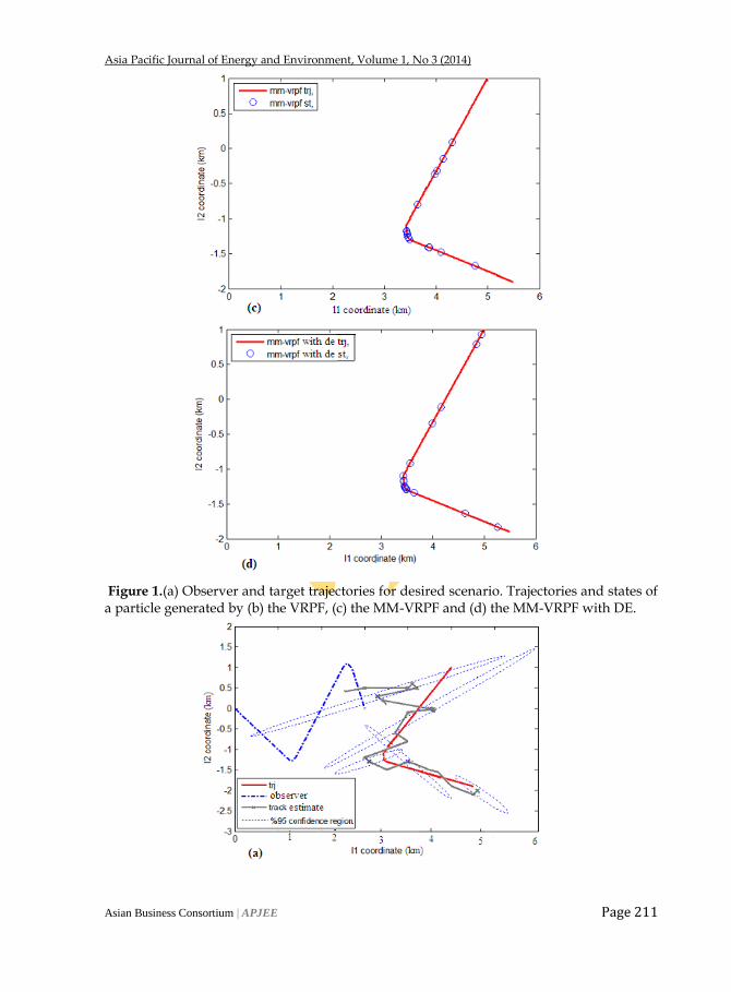
Table 1 represents sojoum time distribution parameters for MM-VRPF and VRPF (Ulker, 2012). This table considers three states; (n=1) for modeling direct form of motion and (n=2,3) to model motion maneuvers of target. The multiple model structure can switch between these states. In Figure 1 sections (b), (c) and (d) explain state arrival the and trajectory points generated by the VRPF, MM-VRPF and MM-VRPF with DE respectively. Figure 1.(c) and (d) show the MM-VRPF and MM-VRPF with DE structure are capable of locating frequent states at bearing region while using a parsimonious state representation for the smooth regions of the trajectory.
Asia Pacific Journal of Energy and Environment, Volume 1, No 3 (2014)
Asian Business Consortium | APJEE Page 210
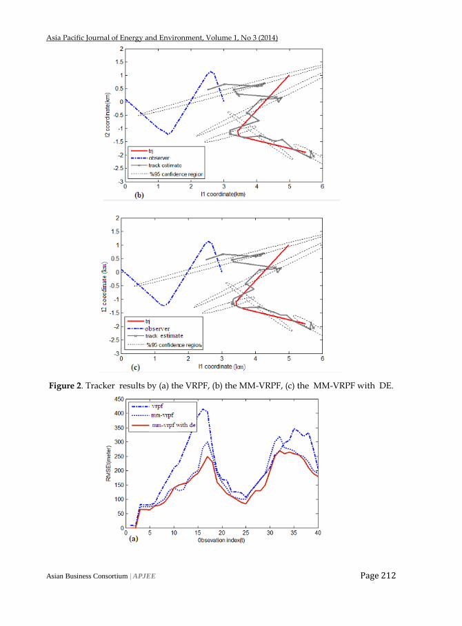
Figure 2 depicts graphs resulted from tracking operation. Figure 2.(a), (b) and (c) respectively illustrate tracking operation based on VRPF, MM-VRPF and MM-VRPF with DE. It is obvious that tracking curve particularly in bearing only regions have much higher quality in MM-VRPF and MM-VRPF with DE than VRPF. Furthermore, focusing on MM-VRPF with DE graph may help us to understand its relative superiority to MM-VRPF technique in path estimation.
Figure 3 shows tRMSE values for three mentioned structures. In figure 3.(a) the diagram
of tRMSE versus 𝑁𝑝 = 2000 and in figure 3.(b) versus 𝑁𝑝 = 4000 are shown using 40
observations for mentioned scenarios. In addition, numerical values of RMSE for 𝑁𝑝 =
2000 and 𝑁𝑝 = 4000 could be seen in table 2. Investigating values presented in table 2
together with tRMSE diagram in figure 3, the superiority of proposed structure could be
concluded.
Asia Pacific Journal of Energy and Environment, Volume 1, No 3 (2014)
Asian Business Consortium | APJEE Page 211
Figure 1.(a) Observer and target trajectories for desired scenario. Trajectories and states of a particle generated by (b) the VRPF, (c) the MM-VRPF and (d) the MM-VRPF with DE.
Asia Pacific Journal of Energy and Environment, Volume 1, No 3 (2014)
Asian Business Consortium | APJEE Page 212
Figure 2. Tracker results by (a) the VRPF, (b) the MM-VRPF, (c) the MM-VRPF with DE.
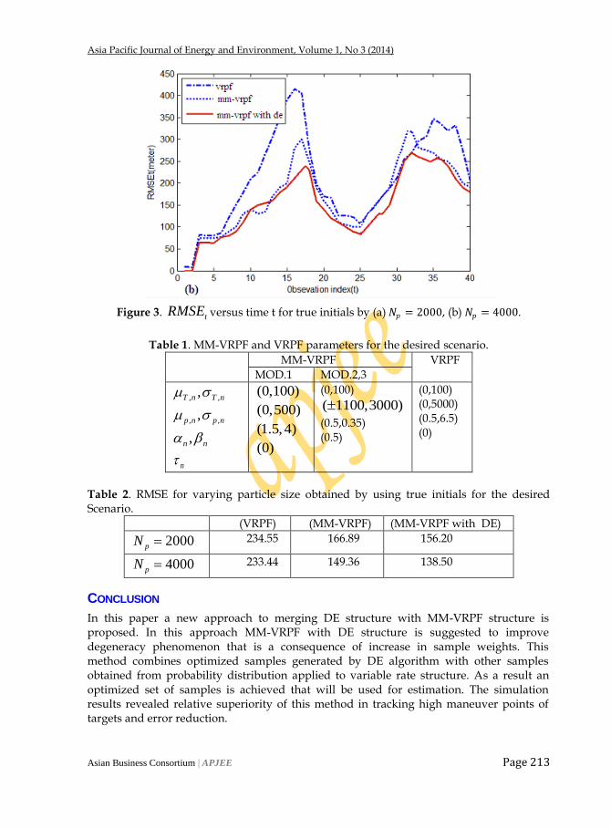
Asia Pacific Journal of Energy and Environment, Volume 1, No 3 (2014)
Asian Business Consortium | APJEE Page 213
Figure 3. tRMSE versus time t for true initials by (a) 𝑁𝑝 = 2000, (b) 𝑁𝑝 = 4000.
Table 1. MM-VRPF and VRPF parameters for the desired scenario.
MM-VRPF VRPF
MOD.1 MOD.2,3
, ,,T n T n
, ,,p n p n
,n n
n
(0,100)
(0,500)
(1.5,4)
(0)
(0,100)
( 1100,3000)
(0.5,0.35) (0.5)
(0,100) (0,5000) (0.5,6.5) (0)
Table 2. RMSE for varying particle size obtained by using true initials for the desired Scenario.
(VRPF) (MM-VRPF) (MM-VRPF with DE)
2000pN 234.55 166.89 156.20
4000pN 233.44 149.36 138.50
CONCLUSION
In this paper a new approach to merging DE structure with MM-VRPF structure is proposed. In this approach MM-VRPF with DE structure is suggested to improve degeneracy phenomenon that is a consequence of increase in sample weights. This method combines optimized samples generated by DE algorithm with other samples obtained from probability distribution applied to variable rate structure. As a result an optimized set of samples is achieved that will be used for estimation. The simulation results revealed relative superiority of this method in tracking high maneuver points of targets and error reduction.

Asia Pacific Journal of Energy and Environment, Volume 1, No 3 (2014)
Asian Business Consortium | APJEE Page 214
REFERENCES
Arulampalam S, Maskell S, Gordon N and Clapp T. A Tutorialon Particle Filters for Online Non-linear/Non-gaussian Bayesian Tracking. IEEE Trans. Signal Process. 2002: 174–188.
Bloomer L, Gray JE. Are more models better?: The effect of the model transition matrix on the IMM filter. In: 4th Southeastern Symp. System Theory; 2002; Huntsville, CANADA. pp. 20–25.
Boers Y. On the Number of Samples to be Drawn in Particle Filtering. IEEE Colloquium on Target Tracking: Algorithms and Applications. 1999: 5/1- 5/6.
Das S, Konar A, Chakraborty U. Improved differential evolution algorithms for handling noisy optimization problems. IEEE Congress on Evolutionary Computation. 2005: 1691–1698.
Doucand R, Capp_e O. Comparison of resampling schemes for particle Filtering. In: Image and Signal Processing and Analysis IEEE 2005 Proceedings of the 4th International Symposium; 2005; USA, IEEE. pp. 64–69.
Doucet A, Godsill SJ, Andrieu C. On sequential Monte Carlo sampling methods for Bayesian filtering. Statistics and computing. 2000: 197–208.
Engelbrecht AP. Computational Intelligence An Introduction 2th Ed.New Jersy. USA: John Wiley and Sons John. 2007.
Fox D. KLD-Sampling: Adaptive Particle Filters. Int. J. Robotics Research. 2003: 985-1003. Godsill SJ, Vermaak J, Ng W, Li JF. Models and Algorithms for Tracking of Maneuvering Objects
Using Variable Rate. proc. IEEE. 2007: 1-28. Gordon N, Salmond D, Smith AFM. Novel Approach to Non-linear and Non-Gaussian Bayesian State
Estimation. Radar and Signal Processing. IEE Proceedings F. Vol. 140. No. 2. 1993: 107–113. Gordon NJ, Salmond DJ, and Smith AFM. Novel approach to nonlinear/non-Gaussian Bayesian
state estimation. in IEE Proceedings. vol. 140. 1993: 107–113. Jilkov VP, Li XR. Online bayesian estimation of transition probabilities for markovian jump systems.
IEEE Trans. Signal Process. 2004: 1620–1630. Li X, Jilkov V. Survey of maneuvering target tracking. Part I: Dynamic models. IEEE Transactions on
Aerospace and Electronic Systems, vol. 39. 2003: 1333–1364. Punch P, Godsill SJ. Dynamical models for tracking with the variable rate particle filter. In: IEEE 15th
International Conference on information fusion; 2012; USA; IEEE. pp. 1769 – 1775. Rahnamayan S, Tizhoosh HR, Salama MMA. Opposition-based differential evolution, IEEE
Transactions on Evolutionary Computation. 2008: 64–79. Ristic B, Arulampalam S, Gordon N. In Beyond Kalman Filter:Particle Filters TrackingApplication.
Artech House Publishers. Boston,Ch. 1–3. 2004: 3–65. Sanjeev Arulampalam M, Ristic B, Gordon N, Mansell T. Bearings-Only Tracking of Manoeuvring
Targets Using Particle Filters. EURASIP Journal on Signal Processing. 2004: 2351-2365. Simon D. Optimal State Estimation Kalman, Hand Non-linear Approaches. New Jersey, USA: John
Wiley and Sons, 2006. Ulker Y, Gunsel B. Multiple model target tracking with variable rate particle filters. Elsevier Journal
on Signal Processing. 2012: 417-429.

Asia Pacific Journal of Energy and Environment, Volume 1, No 3 (2014)
Asian Business Consortium | APJEE Page 215
India’s initiatives on Improving Energy
Efficiency in Aluminium Industries
Piyush Verma1, Alka Verma
2, Anupam Agnihotri
3
1Project Engineer, Bureau of Energy Efficiency, New Delhi, India
2Project Engineer, Energy Efficiency Services Limited, New Delhi, India
3Director, JawaharLal Nehru Aluminium Research Development & Design Centre, Nagpur, India
ABSTRACT
India is an important player in the aluminium, especially because of its abundant bauxite reserves and low-cost skilled manpower. The sector has a significant importance in the growth of Indian economy since the aluminium consumption follows GDP growth curve. Indian aluminium sector is observed as one of the energy intensive sectors with ample scope for improvements in energy efficiency as compared to world standards. The aluminium industries are upgrading themselves by adapting state-of-art technologies, which are more energy-efficient and sustainable in a highly competitive market. These initiatives are further accelerated and motivated by an innovative incentivization scheme (called Perform, Achieve and Trade) of Govt. of India. Currently, the first phase (2012-15) is under implementation, and an unexpected movement towards energy efficiency is envisaged as a result that will ultimately lead towards production of low carbon aluminium for the society. Key words: Industries, Aluminium, PAT, CO2 emission, sustainability
INTRODUCTION
India is the fifth largest producer of bauxite, accounting for 7.4 % of global production in 2012 and the fifth largest producer of alumina. With a 3 % share of global production of primary aluminium, India is among the top ten producers. The 90% increase in primary production since 2000 was mostly driven by demand for aluminium products arising from the aluminium used in transportation, building and electrical segments. With a dramatic increase in the production, the biggest challenge for the aluminium industries is to survive in a highly competitive market in a sustainable and cost-effective manner.
This article is is licensed under a Creative Commons Attribution-NonCommercial 4.0 International License. Attribution-NonCommercial (CC BY-NC) license lets others remix, tweak, and build upon work non-commercially, and although the new works must also acknowledge & be non-commercial.
How to Cite: Verma P, Verma A, Agnihotri A. India’s initiatives on Improving Energy Efficiency in Aluminium Industries Asia Pacific Journal of Energy and Environment. 2014;1(3):215-222.
Source of Support: Nil Conflict of Interest: Non declared
DOI prefix 10.15590/apjee
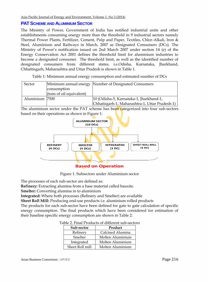
Asia Pacific Journal of Energy and Environment, Volume 1, No 3 (2014)
Asian Business Consortium | APJEE Page 216
PAT SCHEME AND ALUMINIUM SECTOR
The Ministry of Power, Government of India has notified industrial units and other establishments consuming energy more than the threshold in 9 industrial sectors namely Thermal Power Plants, Fertilizer, Cement, Pulp and Paper, Textiles, Chlor-Alkali, Iron & Steel, Aluminium and Railways in March, 2007 as Designated Consumers (DCs). The Ministry of Power‘s notification issued on 2nd March 2007 under section 14 (e) of the Energy Conservation Act 2001 defines the threshold limit for aluminium industries to become a designated consumer. The threshold limit, as well as the identified number of designated consumers from different states, i.e.Odisha, Karnataka, Jharkhand, Chhattisgarh, Maharashtra and Uttar Pradesh is shown in Table 1.
Table 1: Minimum annual energy consumption and estimated number of DCs
Sector Minimum annual energy consumption (tons of oil equivalent)
Number of Designated Consumers
Aluminium 7500 10 (Odisha-5, Karnataka-1, Jharkhand-1, Chhatisgarh-1, Maharashtra-1, Uttar Pradesh-1)
The aluminium sector under the PAT scheme has been categorized into four sub-sectors based on their operations as shown in Figure 1:
Figure 1. Subsectors under Aluminium sector
The processes of each sub-sector are defined as: Refinery: Extracting alumina from a base material called bauxite. Smelter: Converting alumina in to aluminium Integrated: Where both processes (Refinery and Smelter) are available Sheet Roll Mill: Producing end-use products i.e. aluminium rolled products The products for each sub-sector have been defined for gate to gate calculation of specific energy consumption. The final products which have been considered for estimation of their baseline specific energy consumption are shown in Table 2:
Table 2. Final Products of different sub-sectors Sub-sector Product
Refinery Calcined Alumina
Smelter Molten Aluminium
Integrated Molten Aluminium
Sheet Roll mill Molten Aluminium

Asia Pacific Journal of Energy and Environment, Volume 1, No 3 (2014)
Asian Business Consortium | APJEE Page 217
The total reported energy consumption of these designated consumers is about 7.71 million ton of oil equivalent that is around 4.67% of total consumption of industries covered under PAT scheme.
ESTIMATION OF BASELINE AND TARGET SETTING
The target setting for industries under the PAT scheme was a challenging process because of the wide bandwidth of specific energy consumption (SEC) in each of the industrial sectors. Although the wide bandwidth of SEC within an industrial sector is indicative of the large energy-savings potential in that sector but the challenging thing was to assign the energy saving targets to the individual industries as there was a wide variation amongst the plants because of their varying vintage, production capacity, raw material quality, and product-mix . The SEC bandwidth of the aluminium sector is shown in Table 3 where the SEC in most in-efficient plant was 35 times higher than the most efficient plant.
Table 3.SEC Bandwidth of Aluminium Sector
Bandwidth of Sector Bandwidth Index Energy Savings
Min Max Min Max toe
toe/t toe/t
0.183 6.405 1.00 35.00 0.456
Such wide variation also makes it difficult to specify a single benchmark SEC for the sector as a whole: older plants will find the benchmark impossibly high if it is set at the level of newer plants; newer plants will find it trivial if it is set at the level of older plants. The broad bandwidth of SEC within a sector and the inability of all plants to achieve a sectoral benchmark SEC suggest that SEC improvement norms need to be set for individual plants. These SEC improvement targets can be based on the trend of energy consumption and energy-savings potential of the plants. In general, higher the energy efficiency (or, the lower SEC), indicates the lower energy-savings potential. Thus, it is evident that it is not feasible to define a single norm/standard unless there is significant homogeneity amongst units in a sector. Therefore, the energy efficiency improvement targets fixed are ―unit-specific‖. Each industry under the sector has mandated to reduce its SEC by a certain value, based on its current SEC (or baseline SEC) within the sectoral bandwidth. The following target setting methodologies have been adopted in the aluminium sector:
Sectoral target is allocated based on a pro-rate basis of total energy consumption in the aluminum sector among all the eight sectors covered under PAT scheme.
Sub-sectoral target is allocated based on a pro-rata basis of total energy consumption in the sub-sector among the total aluminum sector.
The designated consumer level target is allocated based on a statistical analysis derived from ―Relative SEC‖ concept. This approach was applicable to all the designated consumers of a sub-sector only.
The baseline and target SEC for all the sub-sectors of aluminium sector has been shown in Figure 3:
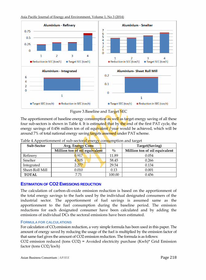
Asia Pacific Journal of Energy and Environment, Volume 1, No 3 (2014)
Asian Business Consortium | APJEE Page 218
Figure 3.Baseline and Target SEC
The apportionment of baseline energy consumption as well as target energy saving of all these four sub-sectors is shown in Table 4. It is estimated that by the end of the first PAT cycle, the energy savings of 0.456 million ton of oil equivalent /year would be achieved, which will be around 7% of total national energy saving targets assessed under PAT scheme.
Table 4.Apportionment of sub-sectoral energy consumption and target
Sub-Sector Avg. Energy Cons
Target(Saving)
Million ton of oil equivalent % Million ton of oil equivalent
Refinery 0.917 11.89 0.054
Smelter 4.505 58.45 0.266
Integrated 2.277 29.54 0.134
Sheet-Roll Mill 0.010 0.13 0.001
TOTAL 7.71 100.00 0.456
ESTIMATION OF CO2 EMISSIONS REDUCTION
The calculation of carbon-di-oxide emission reduction is based on the apportionment of the total energy savings to the fuels used by the individual designated consumers of the industrial sector. The apportionment of fuel savings is assumed same as the apportionment to the fuel consumption during the baseline period. The emission reductions for each designated consumer have been calculated and by adding the emissions of individual DCs the sectoral emissions have been estimated.
FORMULA FOR CALCULATIONS For calculation of CO2 emission reduction, a very simple formula has been used in this paper. The amount of energy saved by reducing the usage of the fuel is multiplied by the emission factor of that same fuel gives the amount of CO2 emission reduction. The formula is as follows: CO2 emission reduced (tons CO2) = Avoided electricity purchase (Kwh)* Grid Emission factor (tons CO2/kwh)
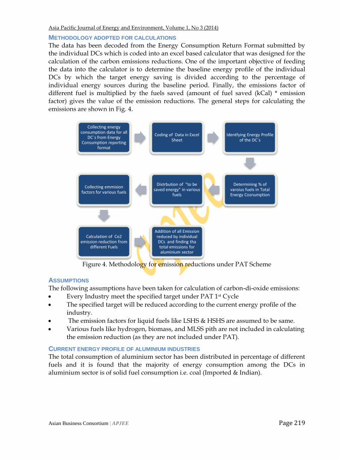
Asia Pacific Journal of Energy and Environment, Volume 1, No 3 (2014)
Asian Business Consortium | APJEE Page 219
METHODOLOGY ADOPTED FOR CALCULATIONS The data has been decoded from the Energy Consumption Return Format submitted by the individual DCs which is coded into an excel based calculator that was designed for the calculation of the carbon emissions reductions. One of the important objective of feeding the data into the calculator is to determine the baseline energy profile of the individual DCs by which the target energy saving is divided according to the percentage of individual energy sources during the baseline period. Finally, the emissions factor of different fuel is multiplied by the fuels saved (amount of fuel saved (kCal) * emission factor) gives the value of the emission reductions. The general steps for calculating the emissions are shown in Fig. 4.
Figure 4. Methodology for emission reductions under PAT Scheme
ASSUMPTIONS The following assumptions have been taken for calculation of carbon-di-oxide emissions:
Every Industry meet the specified target under PAT 1st Cycle
The specified target will be reduced according to the current energy profile of the industry.
The emission factors for liquid fuels like LSHS & HSHS are assumed to be same.
Various fuels like hydrogen, biomass, and MLSS pith are not included in calculating the emission reduction (as they are not included under PAT).
CURRENT ENERGY PROFILE OF ALUMINIUM INDUSTRIES The total consumption of aluminium sector has been distributed in percentage of different fuels and it is found that the majority of energy consumption among the DCs in aluminium sector is of solid fuel consumption i.e. coal (Imported & Indian).
Collecting energy consumption data for all
DC`s from Energy Consumption reporting
format
Coding of Data in Excel Sheet
Identfying Energy Profile of the DC`s
Determining % of varoius fuels in Total Energy Cosnumption
Distrbution of "to be saved energy" in various
fuels
Collecting emmision factors for various fuels
Calculation of Co2 emission reduction from
different Fuels
Addition of all Emission reduced by individual DCs and finding tha total emissions for aluminium sector
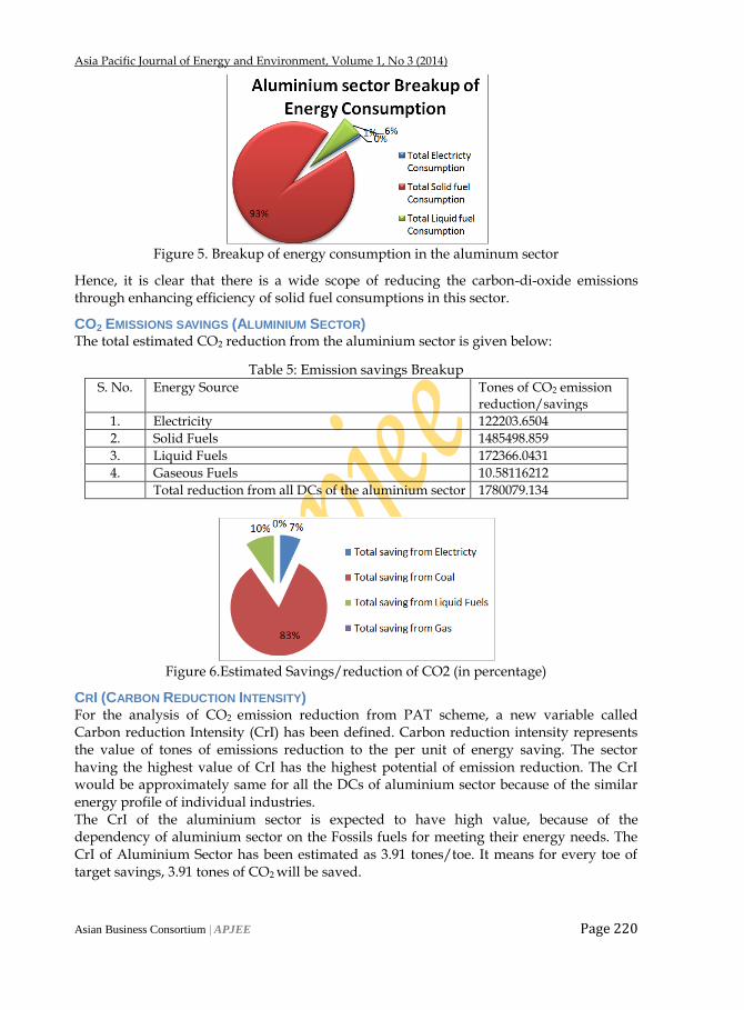
Asia Pacific Journal of Energy and Environment, Volume 1, No 3 (2014)
Asian Business Consortium | APJEE Page 220
Figure 5. Breakup of energy consumption in the aluminum sector
Hence, it is clear that there is a wide scope of reducing the carbon-di-oxide emissions through enhancing efficiency of solid fuel consumptions in this sector.
CO2 EMISSIONS SAVINGS (ALUMINIUM SECTOR) The total estimated CO2 reduction from the aluminium sector is given below:
Table 5: Emission savings Breakup S. No. Energy Source Tones of CO2 emission
reduction/savings
1. Electricity 122203.6504
2. Solid Fuels 1485498.859
3. Liquid Fuels 172366.0431
4. Gaseous Fuels 10.58116212
Total reduction from all DCs of the aluminium sector 1780079.134
Figure 6.Estimated Savings/reduction of CO2 (in percentage)
CRI (CARBON REDUCTION INTENSITY) For the analysis of CO2 emission reduction from PAT scheme, a new variable called Carbon reduction Intensity (CrI) has been defined. Carbon reduction intensity represents the value of tones of emissions reduction to the per unit of energy saving. The sector having the highest value of CrI has the highest potential of emission reduction. The CrI would be approximately same for all the DCs of aluminium sector because of the similar energy profile of individual industries. The CrI of the aluminium sector is expected to have high value, because of the dependency of aluminium sector on the Fossils fuels for meeting their energy needs. The CrI of Aluminium Sector has been estimated as 3.91 tones/toe. It means for every toe of target savings, 3.91 tones of CO2 will be saved.
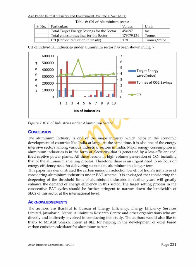
Asia Pacific Journal of Energy and Environment, Volume 1, No 3 (2014)
Asian Business Consortium | APJEE Page 221
Table 6: CrI of Aluminium sector S. No. Particulars Values Units
Total Target Energy Savings for the Sector 454997 toe
Total emission savings for the Sector 178079.134 Tonnes
CrI (Carbon reduction Intensity) 3.91 Tonnes/mtoe
CrI of individual industries under aluminium sector has been shown in Fig. 7.
Figure 7.1CrI of Industries under Aluminium Sector
CONCLUSION
The aluminium industry is one of the major industry which helps in the economic development of countries like India at large. At the same time, it is also one of the energy intensive sectors among various industrial sectors in India. Major energy consumption in aluminium industries is in the form of electricity that is generated by a less-efficient coal fired captive power plants. All these results in high volume generation of CO2 including that of the aluminium smelting process. Therefore, there is an urgent need to re-focus on energy efficiency need for delivering sustainable aluminium in a longer term. This paper has demonstrated the carbon emission reduction benefit of India‘s initiatives of considering aluminium industries under PAT scheme. It is envisaged that considering the deepening of the threshold limit of aluminium industries in further years will greatly enhance the demand of energy efficiency in this sector. The target setting process in the consecutive PAT cycles should be further stringent to narrow down the bandwidth of SECs of this sector at the international level.
ACKNOWLEDGEMENTS
The authors are thankful to Bureau of Energy Efficiency, Energy Efficiency Services Limited, Jawaharlal Nehru Aluminium Research Centre and other organizations who are directly and indirectly involved in conducting this study. The authors would also like to thank to Mr.Atik Shiekh, Intern at BEE for helping in the development of excel based carbon emission calculator for aluminium sector.
0
1
2
3
4
5
6
7
0
100000
200000
300000
400000
500000
600000
1 2 3 4 5 6 7 8 9 10
T
o
n
n
e
s
No of Industries
Target Energy saved(mtoe)
Tonnes of CO2 Savings
Cri
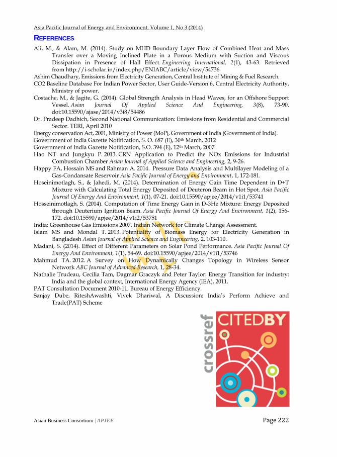
Asia Pacific Journal of Energy and Environment, Volume 1, No 3 (2014)
Asian Business Consortium | APJEE Page 222
REFERENCES
Ali, M., & Alam, M. (2014). Study on MHD Boundary Layer Flow of Combined Heat and Mass Transfer over a Moving Inclined Plate in a Porous Medium with Suction and Viscous Dissipation in Presence of Hall Effect. Engineering International, 2(1), 43-63. Retrieved from http://i-scholar.in/index.php/ENIABC/article/view/54736
Ashim Chaudhary, Emissions from Electricity Generation, Central Institute of Mining & Fuel Research. CO2 Baseline Database For Indian Power Sector, User Guide-Version 6, Central Electricity Authority,
Ministry of power. Costache, M., & Jagite, G. (2014). Global Strength Analysis in Head Waves, for an Offshore Support
Vessel. Asian Journal Of Applied Science And Engineering, 3(8), 73-90. doi:10.15590/ajase/2014/v3i8/54486
Dr. Pradeep Dadhich, Second National Communication: Emissions from Residential and Commercial Sector. TERI, April 2010
Energy conservation Act, 2001, Ministry of Power (MoP), Government of India (Government of India). Government of India Gazette Notification, S. O. 687 (E), 30th March, 2012 Government of India Gazette Notification, S.O. 394 (E), 12th March, 2007 Hao NT and Jungkyu P. 2013. CRN Application to Predict the NOx Emissions for Industrial
Combustion Chamber Asian Journal of Applied Science and Engineering, 2, 9-26. Happy FA, Hossain MS and Rahman A. 2014. Pressure Data Analysis and Multilayer Modeling of a
Gas-Condansate Reservoir Asia Pacific Journal of Energy and Environment, 1, 172-181. Hoseinimotlagh, S., & Jahedi, M. (2014). Determination of Energy Gain Time Dependent in D+T
Mixture with Calculating Total Energy Deposited of Deuteron Beam in Hot Spot. Asia Pacific Journal Of Energy And Environment, 1(1), 07-21. doi:10.15590/apjee/2014/v1i1/53741
Hosseinimotlagh, S. (2014). Computation of Time Energy Gain in D-3He Mixture: Energy Deposited through Deuterium Ignition Beam. Asia Pacific Journal Of Energy And Environment, 1(2), 156-172. doi:10.15590/apjee/2014/v1i2/53751
India: Greenhouse Gas Emissions 2007, Indian Network for Climate Change Assessment. Islam MS and Mondal T. 2013. Potentiality of Biomass Energy for Electricity Generation in
Bangladesh Asian Journal of Applied Science and Engineering, 2, 103-110. Madani, S. (2014). Effect of Different Parameters on Solar Pond Performance. Asia Pacific Journal Of
Energy And Environment, 1(1), 54-69. doi:10.15590/apjee/2014/v1i1/53746 Mahmud TA. 2012. A Survey on How Dynamically Changes Topology in Wireless Sensor
Network ABC Journal of Advanced Research, 1, 28-34. Nathalie Trudeau, Cecilia Tam, Dagmar Graczyk and Peter Taylor: Energy Transition for industry:
India and the global context, International Energy Agency (IEA), 2011. PAT Consultation Document 2010-11, Bureau of Energy Efficiency. Sanjay Dube, RiteshAwashti, Vivek Dhariwal, A Discussion: India‘s Perform Achieve and
Trade(PAT) Scheme

Asia Pacific Journal of Energy and Environment, Volume 1, No 3 (2014)
Asian Business Consortium | APJEE Page 223
Off Pantai Dalam, Kuala Lampur, Malaysia Rd 4, Shyamoli, Dhaka-1207, Bangladesh
3900 Woodhue Place, Alexandria, VA 22309, USA
www.abcreorg.weebly.com / www.abcjournals.net
Asian Business Consortium (ABC) is a multi-disciplinary research, training, publishing, digital library supporting and service house. Though founded in 2010 as the Business and Computing organization of Asia, it was reconstituted as the ABC in 2011. It has been working for creating and nurturing talents in USA, Malaysia and Bangladesh since its inception. As ABC is going global, it intends to open chapters in Australia, Germany, Japan, Pakistan, and other Asian countries in near future. The objectives of consortium are solely centered round the welfare and humane attitude of the founders who enthusiastically took up this noble cause and materialized it with a view to promote research and educational activities for the encouragement of scholars to develop their knowledge, to publish their analysis oriented scientific researches in international Journals, books, the task of organizing workshops, seminars, conferences, training, personality development programs and allied services. In addition to research activities, ABC provides a good number of scholarships to the poor and meritorious students at various levels of education throughout the world. It plays an important role in the field of research by funding research projects and publishing the research papers. This consortium will unquestionably become the mouth-piece of the dark horses and unacknowledged scholar whose endowed and commendable contributions shall be provided an outlet keeping in mind the greater good of the larger society of the world. ABC runs the following international referred journals for creating a platform to share the thoughts of professionals, scholars and academicians throughout the world.
ABC Publications (ABC Journals)
Asian Accounting and Auditing Advancement (4A Journal)
Asian Business Review (ABR)
Asian Journal of Applied Sciences and Engineering (AJASE)
Global Disclosure of Economics and Business (GDEB)
ABC Journal of Advanced Research (ABC-JAR)
International Journal of Reciprocal Symmetry and Theoretical Physics (IJRSTP)
American Journal of Trade and Policy (AJTP)
Asian Journal of Humanity, Art and Literature (AJHAL)
Malaysian Journal of Medical and Biological Research (MJMBR)
Asia Pacific Journal of Energy and Environment (APJEE)
Engineering International (EI)
ABC Research Alert (Online) Each journal home page provides specific information for potential authors and subscribers. Open access policy, the quick review process, rich editorial boards and quality publications have already made ABC Journals unique. ABC Journals are published under the direct supervisions of renowned academicians of the world. Collaboration in Conference: ABC considers high-quality conference papers for publication. Please contact us for detailed information. Collaboration in Publishing: If you like to start writing a book, propose a new journal or advertise in ABC journals, please feel free to contact us.