AP Microeconomics Full Review - North Allegheny · AP ® Microeconomics Full Review . VERSION 2 ... Around 18% and 15% of people get 5s on the AP Micro and AP Macro ... Economics

Primary Works Consulted:

1. Notes from Mrs. Joelle Keats’, Mr. Nathan Tengowski, and Mr. Jason Mohr’s AP Economics Classes

2. Cracking the AP Economics Exams (2015) 3. ACDCecon: http://www.acdcecon.com/#!ap-econ/c18qp 4. Crash Course Economics: https://www.youtube.com/user/crashcourse

AP and Advanced Placement are registered trademarks of the College Board, which does not sponsor or endorse this product.

Updated:

2015-2016

AP® Microeconomics Full Review

VERSION 2.0

AUTHOR: GABE REN

http://www.acdcecon.com/#!ap-econ/c18qp

https://www.youtube.com/user/crashcourse

Shared Folder: http://bit.ly/AP_ECON

AP Microeconomics Full Review Page 1 of 56

Table of Contents Please Read/Background Info................................................................................................................... 5

About the Exams ....................................................................................................................................... 5

Resources .................................................................................................................................................. 6

Tips ........................................................................................................................................................... 6

Key for Abbreviations .............................................................................................................................. 7

Micro Unit 1: Basic Economic Concepts ................................................................................................. 8

Scarcity ................................................................................................................................................. 8

Factors of Production (Inputs): LLCE .................................................................................................. 8

EXAMPLE: Factors of Production – Donut Shop ............................................................................... 8

Opportunity Costs ................................................................................................................................. 9

GRAPH: Production Possibilities Curve/Frontier (PPC/PPF) with Specialization .............................. 9

GRAPH: Production Possibilities Curve/Frontier (PPC/PPF) without Specialization....................... 10

GRAPH: Capital Goods vs. Consumption Goods on a PPC/PPF ...................................................... 11

Specialization and Comparative Advantage ....................................................................................... 12

EXAMPLE: Absolute and Comparative Advantages ......................................................................... 12

Three Important Questions for any Economy .................................................................................... 13

Systems of Government ...................................................................................................................... 14

Micro Unit 2: The Nature and Functions of Product Markets: Supply and Demand ............................. 15

GRAPH: Demand Curve .................................................................................................................... 15

EXAMPLE: Summation of Individual Demand Curves .................................................................... 16

GRAPH: Marginal Utility (MU) vs. Total Utility .............................................................................. 17

GRAPH: Supply Curve....................................................................................................................... 18

EXAMPLE: Summation of Individual Supply Curves ...................................................................... 19

GRAPH: Supply and Demand ............................................................................................................ 19

http://bit.ly/AP_ECON

EXAMPLE: Supply or Demand Shifting ........................................................................................... 20

EXAMPLE: Supply and Demand Shifting ......................................................................................... 21

GRAPH: Consumer and Producer Surplus ......................................................................................... 21

GRAPH: Price Ceilings ...................................................................................................................... 22

GRAPH: Price Floors ......................................................................................................................... 22

EXAMPLE: Tax on Buyers (Demand) ............................................................................................... 23

EXAMPLE: Tax on Suppliers (Supply) ............................................................................................. 24

Micro Unit 3: Production, Costs, and Elasticity ..................................................................................... 25

Elasticity ............................................................................................................................................. 25

Price Elasticity of Demand ................................................................................................................. 25

GRAPH: Price Elasticity of Demand ................................................................................................. 26

EXAMPLE: Total Revenue Test ........................................................................................................ 27

Price Elasticity of Supply ................................................................................................................... 27

Income Elasticity of Demand ............................................................................................................. 28

Cross-Price Elasticity of Demand ....................................................................................................... 28

GRAPH: Marginal Product and Total Product ................................................................................... 29

GRAPH: Marginal Cost and Total Cost ............................................................................................. 30

Short Run vs. Long Run ..................................................................................................................... 31

GRAPH: Economies of Scale ............................................................................................................. 32

Micro Unit 4: Perfect Competition ......................................................................................................... 33

Key Terms .......................................................................................................................................... 33

EXAMPLE: Decreasing Cost Industry (less common) ...................................................................... 34

GRAPH: Perfect Competition ............................................................................................................ 35

GRAPH: Total Cost and Total Revenue ............................................................................................. 36

GRAPH: Perfect Competition – Profit Maximizing Firm .................................................................. 37



GRAPH: Shut Down Decision ........................................................................................................... 38

Micro Unit 5: Monopolies ...................................................................................................................... 39

GRAPH: Monopoly ............................................................................................................................ 39

Price Discrimination ........................................................................................................................... 40

GRAPH: Monopoly – Perfect Price Discrimination .......................................................................... 40

GRAPH: Monopoly – Perfect Price Discrimination w/Differing Demand Elasticities ..................... 41

EXAMPLE: Government Policy towards Imperfect Competition ..................................................... 41

GRAPH: Natural Monopoly ............................................................................................................... 42

Micro Unit 6: Monopolistic Competition and Oligopolies ..................................................................... 43

GRAPH: Monopolistic Competition .................................................................................................. 43

Oligopoly ............................................................................................................................................ 44

Game Theory ...................................................................................................................................... 44

EXAMPLE: Payoff Matrix – Dominant Strategy Equilibrium .......................................................... 45

EXAMPLE: Payoff Matrix – Non-Dominant Strategy Equilibrium .................................................. 46

Bilateral Monopoly (less common) .................................................................................................... 46

SUMMARY: Market Structures ............................................................................................................. 47

Micro Unit 7: Factor Markets ................................................................................................................. 48

EXAMPLE: Factor Markets – Ice Cream Machines .......................................................................... 48

GRAPH: Marginal Revenue Product of Labor ................................................................................... 48

GRAPH: Perfectly Competition – Labor Market ............................................................................... 49

GRAPH: Monopsony.......................................................................................................................... 50

Unions (less common) ........................................................................................................................ 51

Micro Unit 8: Market Failures and the Role of Government ................................................................. 52

Market Failures ................................................................................................................................... 52

Externalities ........................................................................................................................................ 52


EXAMPLE: Negative Externality ...................................................................................................... 53

EXAMPLE: Positive Externality ........................................................................................................ 53

Public Goods ....................................................................................................................................... 54

Antitrust Legislation (less common) .................................................................................................. 54

Measures of Market Power (less common) ........................................................................................ 55

GRAPH: Lorenz Curve ....................................................................................................................... 55

Poverty and Taxes ............................................................................................................................... 56



Please Read/Background Info

I. This resource is not meant to teach you economics; rather it is meant to serve as a concise guide for

you to review economic knowledge you have already learned (translation: you still need to pay

attention in class)

II. Very few parts of this study guide are bolded so pay special attention to bolded sections

III. (less common) indicates material that can, but rarely, appears on the AP test

IV. GRAPH: or DIAGRAM: indicates the section has an accompanying graph or diagram

V. SUMMARY: provides a short summary of a section’s material

VI. This is the full version of the study guide. Other resources including the condensed version can be

found here: http://bit.ly/1UqPiBi

About the Exams

Around 18% and 15% of people get 5s on the AP Micro and AP Macro tests, respectively1

Shoot for an 80% to 85% on both the MC and FR sections for a 5

I. 60 multiple choice

a. 70 minutes

b. 66% of total score

II. 3 free response

a. 60 minutes

i. 10 minute reading/planning period

1. May begin the test during this time

ii. 50 minute solving period

b. 33% of total score

i. Long FR counts for ½ of this percentage

1. Spend around 25 minutes

ii. Two short FR count for ¼ of this percentage

1. Spend around 25 minutes

1 Data from the 2015 AP Microeconomics and AP Macroeconomics Tests


http://bit.ly/1UqPiBi

Resources

I. AP Central

a. Contains course description with practice MC questions and past FR questions

b. Micro Homepage:

http://apcentral.collegeboard.com/apc/public/courses/teachers_corner/2121.html

c. Micro FR:

http://apcentral.collegeboard.com/apc/members/exam/exam_information/2084.html

d. Macro Homepage:


e. Macro FR:


II. ACDCecon (Mr. Clifford)

a. http://www.acdcecon.com/#!ap-econ/c18qp

b. Micro cumulative video review: https://www.youtube.com/watch?v=JRlREpsr348

c. Macro cumulative video review: https://www.youtube.com/watch?v=e18RXFFoL9c

III. Crash Course Economics

a. https://www.youtube.com/user/crashcourse

Tips

These are applicable to both exams, unless stated otherwise.

I. Multiple choice section

a. Types of questions

i. Economic policy

ii. Graphs

iii. True vs. false statements

b. Use the process of elimination

c. Stick with your gut feeling

d. Two pass system

i. Skip the questions you aren’t comfortable with





http://www.acdcecon.com/#!ap-econ/c18qp

https://www.youtube.com/watch?v=JRlREpsr348

https://www.youtube.com/watch?v=e18RXFFoL9c

https://www.youtube.com/user/crashcourse



1. Come back to them later if you have time

ii. Use the letter of the day strategy

1. Guess using the same answer choice

e. No penalty for guessing

II. Free response section

a. Determine which economic tools the question is asking about

b. Always draw graphs even if they aren’t explicitly asked for

i. Label every line and axis

ii. Graphs will help you avoid making silly mistakes

c. Don’t skip steps in your explanation

i. Bad answer: expansionary monetary policy shifts AD out

ii. Good answer: expansionary monetary policy shifts the money supply curve to the

right, thus lowering interest rates which attracts more investment and shifts AD out

d. Don’t say unnecessary stuff though

i. AP graders will take off points for incorrect extraneous information

e. As a blanket statement, always think in terms of marginal cost = marginal benefit

Key for Abbreviations

I. MC = multiple choice

II. FR = free response

III. PL = price level

IV. F.O.P. = factors of production

V. Rightward shift = outward shift

VI. Leftward shift = inward shift

VII. SR = short run

VIII. LR = long run

IX. e = subscript e = equilibrium

X. 𝚫𝚫 = delta = change in

XI. Fed = federal reserve = central bank

XII. Ceteris paribus = all other things being held equal


Micro Unit 1: Basic Economic Concepts

Economics is the study of how to allocate scarce resources among competing ends.

Microeconomics analyzes the market behavior of individual consumers and firms in an attempt to

understand the decision-making process of firms and households.

Scarcity

I. Occurs b/c our unlimited desire for goods and services exceeds our limited ability to produce them

due to constraints on time and resources

Factors of Production (Inputs): LLCE

I. Land (natural resources)

a. Any productive resource existing in nature

b. E.g. water, wind, mineral deposits

II. Labor

a. Physical and mental effort of people

III. Capital

a. Manufactured goods that can be used in the production process

b. E.g. tools, equipment, buildings, machinery

c. Human capital (less common)

i. Knowledge and skills acquired through training and experience

IV. Entrepreneurship

a. Ability to identify opportunities and organize production

b. Willingness to accept risk in the pursuit of rewards

EXAMPLE: Factors of Production – Donut Shop

I. Land

a. Land and rain provide wheat for the dough

II. Labor

a. People making and selling the donuts



III. Capital

a. Building, ovens

IV. Entrepreneurship

a. Shop-owner took risks to open a business

Opportunity Costs

I. Value of the best alternative sacrificed as compared to what actually takes place

II. Implicit costs

a. Forgone benefits of any single transaction

b. E.g. time and effort an owner puts into maintaining a company, rather than expanding it

III. Explicit costs

a. Expenses that are paid with cash or equivalent

b. E.g. wages to workers, electricity bill

GRAPH: Production Possibilities Curve/Frontier (PPC/PPF) with Specialization

I. Illustrates the choices an economy faces when deciding to produce one good over another

II. Point A

a. Outside the frontier

b. Currently unobtainable


III. Point B

a. Inside the frontier

b. Obtainable but inefficient

IV. Point C

a. On the frontier

b. Efficiency occurs at all points on the frontier

i. Economy is using all of its resources productively

V. Effects of specialization on the PPC/PPF (less common)

a. Assume our economy is only producing chairs

b. The initial opportunity cost of producing one birdcage is small, only 0.25 chairs

c. However, as we begin to produce more birdcages, the opportunity cost rises

d. This is b/c the resources that are used to produce birdcages are less and less specialized for

birdcage production and more and more specialized for chair production

GRAPH: Production Possibilities Curve/Frontier (PPC/PPF) without Specialization

I. Effect of no specialization on the PPC/PPF (less common)

a. Economy must allocate its resources between two goods that involves no specialization of

resources; skills, tools etc. to produce the two goods may be identical



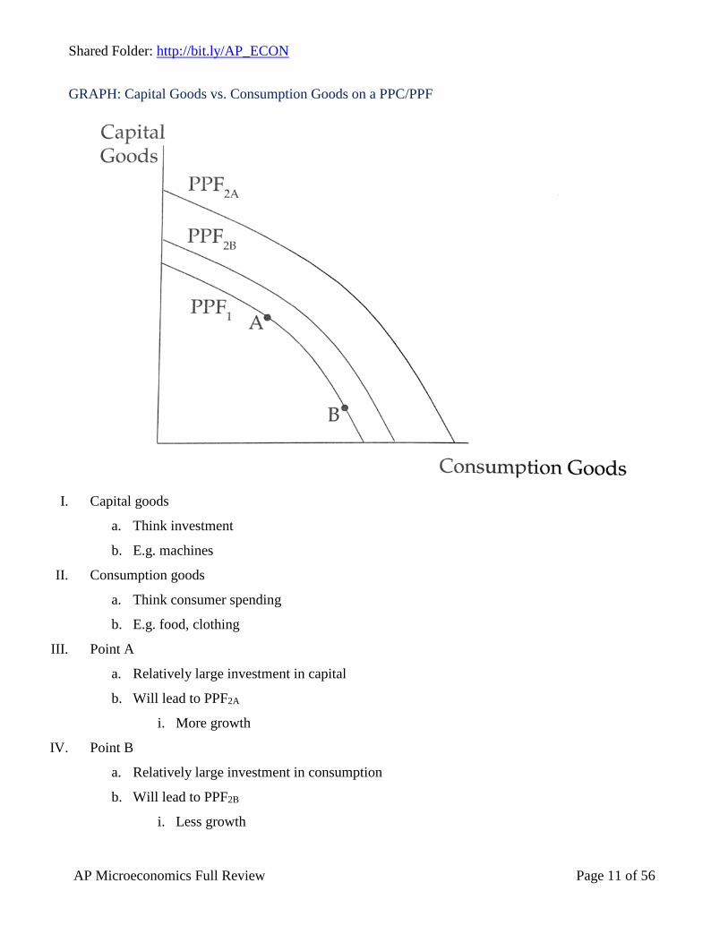
GRAPH: Capital Goods vs. Consumption Goods on a PPC/PPF

I. Capital goods

a. Think investment

b. E.g. machines

II. Consumption goods

a. Think consumer spending

b. E.g. food, clothing

III. Point A

a. Relatively large investment in capital

b. Will lead to PPF2A

i. More growth

IV. Point B

a. Relatively large investment in consumption

b. Will lead to PPF2B

i. Less growth


Specialization and Comparative Advantage

I. Specialization results from people having different skills and leads to increased productivity

II. Division of labor

a. Permits people to develop expertise in the task(s) they concentrate on

III. Absolute advantage

a. Production of a good requires fewer resources per unit than another country

b. Just b/c a country has an absolute advantage, it doesn’t mean that the country

necessarily benefits the most from producing that good

IV. Comparative advantage

a. Production of a good has a lower opportunity cost (of another good) than another country

b. Countries will benefit from specialization if one country has a comparative advantage

in one good, and the other country has a comparative advantage in the other good

V. Trade ends up benefiting both countries

EXAMPLE: Absolute and Comparative Advantages

I. Consider Brazil and Mexico in the production of coffee and broccoli

II. Brazil has an absolute advantage in both producing coffee and broccoli

III. Let’s calculate the comparative advantages for each country

a. 𝐵𝐵𝐵𝐵𝐵𝐵𝐵𝐵𝐵𝐵𝐵𝐵𝑜𝑜𝑜𝑜𝑜𝑜𝑜𝑜𝑜𝑜𝑜𝑜𝑜𝑜𝑜𝑜𝑜𝑜𝑜𝑜𝑜𝑜 𝑐𝑐𝑜𝑜𝑐𝑐𝑜𝑜 𝑓𝑓𝑜𝑜𝑜𝑜 1 𝑐𝑐𝑜𝑜𝑓𝑓𝑓𝑓𝑐𝑐𝑐𝑐 = 1 𝑏𝑏𝐵𝐵𝑏𝑏𝑏𝑏𝑏𝑏𝑏𝑏𝐵𝐵𝐵𝐵

b. 𝐵𝐵𝐵𝐵𝐵𝐵𝐵𝐵𝐵𝐵𝐵𝐵𝑜𝑜𝑜𝑜𝑜𝑜𝑜𝑜𝑜𝑜𝑜𝑜𝑜𝑜𝑜𝑜𝑜𝑜𝑜𝑜𝑜𝑜 𝑐𝑐𝑜𝑜𝑐𝑐𝑜𝑜 𝑓𝑓𝑜𝑜𝑜𝑜 1 𝑏𝑏𝑜𝑜𝑜𝑜𝑐𝑐𝑐𝑐𝑜𝑜𝑏𝑏𝑜𝑜 = 1 𝑏𝑏𝑏𝑏𝑐𝑐𝑐𝑐𝑐𝑐𝑐𝑐

c. 𝑀𝑀𝑐𝑐𝑀𝑀𝐵𝐵𝑏𝑏𝑏𝑏𝑜𝑜𝑜𝑜𝑜𝑜𝑜𝑜𝑜𝑜𝑜𝑜𝑜𝑜𝑜𝑜𝑜𝑜𝑜𝑜𝑜𝑜 𝑐𝑐𝑜𝑜𝑐𝑐𝑜𝑜 𝑓𝑓𝑜𝑜𝑜𝑜 1 𝑐𝑐𝑜𝑜𝑓𝑓𝑓𝑓𝑐𝑐𝑐𝑐 = 0.5 𝑏𝑏𝐵𝐵𝑏𝑏𝑏𝑏𝑏𝑏𝑏𝑏𝐵𝐵𝐵𝐵𝑏𝑏

d. 𝑀𝑀𝑐𝑐𝑀𝑀𝐵𝐵𝑏𝑏𝑏𝑏𝑜𝑜𝑜𝑜𝑜𝑜𝑜𝑜𝑜𝑜𝑜𝑜𝑜𝑜𝑜𝑜𝑜𝑜𝑜𝑜𝑜𝑜 𝑐𝑐𝑜𝑜𝑐𝑐𝑜𝑜 𝑓𝑓𝑜𝑜𝑜𝑜 1 𝑏𝑏𝑜𝑜𝑜𝑜𝑐𝑐𝑐𝑐𝑜𝑜𝑏𝑏𝑜𝑜 = 2 𝑏𝑏𝑏𝑏𝑐𝑐𝑐𝑐𝑐𝑐𝑐𝑐𝑏𝑏



IV. Mexico has a comparative advantage in the production of coffee

V. Brazil has a comparative advantage in the production of broccoli

VI. Thus, both of these countries can benefit from trade

Three Important Questions for any Economy

I. What goods and services will be produced?

a. Seeking allocative efficiency

i. P = MC

b. Output reflects the needs and wants of consumers

II. How much of each input will be used in the production of each good?

a. Seeking productive efficiency

i. P = minimum ATC

b. Marginal products of labor and capital (less common)

i. Firm only uses labor and capital to produce goods

ii. 𝑃𝑃𝐵𝐵𝐵𝐵𝑏𝑏𝑐𝑐 𝑏𝑏𝑐𝑐 𝐵𝐵𝐵𝐵𝑏𝑏𝑏𝑏𝐵𝐵 (𝑃𝑃𝐿𝐿) = 𝑤𝑤𝐵𝐵𝑤𝑤𝑐𝑐 (𝑤𝑤)

iii. 𝑃𝑃𝐵𝐵𝐵𝐵𝑏𝑏𝑐𝑐 𝑏𝑏𝑐𝑐 𝑏𝑏𝐵𝐵𝑐𝑐𝐵𝐵𝑐𝑐𝐵𝐵𝐵𝐵 (𝑃𝑃𝐾𝐾) = 𝐵𝐵𝑐𝑐𝑟𝑟𝑐𝑐𝐵𝐵𝐵𝐵 𝐵𝐵𝐵𝐵𝑐𝑐𝑐𝑐 (𝐵𝐵)

iv. 𝑀𝑀 = 𝑚𝑚𝐵𝐵𝐵𝐵𝑤𝑤𝐵𝐵𝑟𝑟𝐵𝐵𝐵𝐵

v. We want 𝑀𝑀𝑃𝑃𝐾𝐾𝑜𝑜

= 𝑀𝑀𝑃𝑃𝐿𝐿𝑤𝑤

1. If one side is too “heavy,” a firm will invest more into the other side and

decreases investment into the current side to achieve productive efficiency

III. Who will receive the final products?

a. Seeking distributive efficiency (less common)

i. Marginal rate of substitution (MRS) = 𝑃𝑃𝐴𝐴𝑃𝑃𝐵𝐵

= 𝑀𝑀𝑈𝑈𝐴𝐴𝑀𝑀𝑈𝑈𝐵𝐵

ii. Formal condition for distributive efficiency is when every consumer’s MRS is equal

b. Those who place the highest relative value on goods receive them

c. Marginal utilities

i. 𝑀𝑀𝐵𝐵𝐵𝐵𝑤𝑤𝐵𝐵𝑟𝑟𝐵𝐵𝐵𝐵 𝑢𝑢𝑐𝑐𝐵𝐵𝐵𝐵𝐵𝐵𝑐𝑐𝑢𝑢 = 𝑀𝑀𝑀𝑀

ii. We want 𝑀𝑀𝑈𝑈𝑓𝑓𝑓𝑓𝑓𝑓𝑓𝑓𝑃𝑃𝑓𝑓𝑓𝑓𝑓𝑓𝑓𝑓

= 𝑀𝑀𝑈𝑈𝑐𝑐𝑐𝑐𝑓𝑓𝑐𝑐ℎ𝑒𝑒𝑒𝑒𝑃𝑃𝑐𝑐𝑐𝑐𝑓𝑓𝑐𝑐ℎ𝑒𝑒𝑒𝑒

1. This is where utility is maximized


Systems of Government

I. Communism

a. Minimize imbalance in wealth via the collective ownership of property

b. Lacks incentives for extra effort, risk taking, and innovation

c. Wages determined by the gov.

d. Particularly vulnerable to corruption as the gov. plays the central role in allocating

resources; only one political party

II. Socialism

a. Minimize imbalance in wealth

b. Lacks incentives for extra effort, risk taking, and innovation

c. Wages determined by negotiations between trade unions and managers

d. Multiple political parties

III. Capitalism

a. Pursuit of individual profit

b. Private individuals control the factors of production

c. Wages determined by negotiations between trade unions and managers

d. Market forces of supply and demand determine the allocation of resources

e. Gov. can regulate business and provide tax-supported social benefits



Micro Unit 2: The Nature and Functions of Product Markets: Supply and Demand

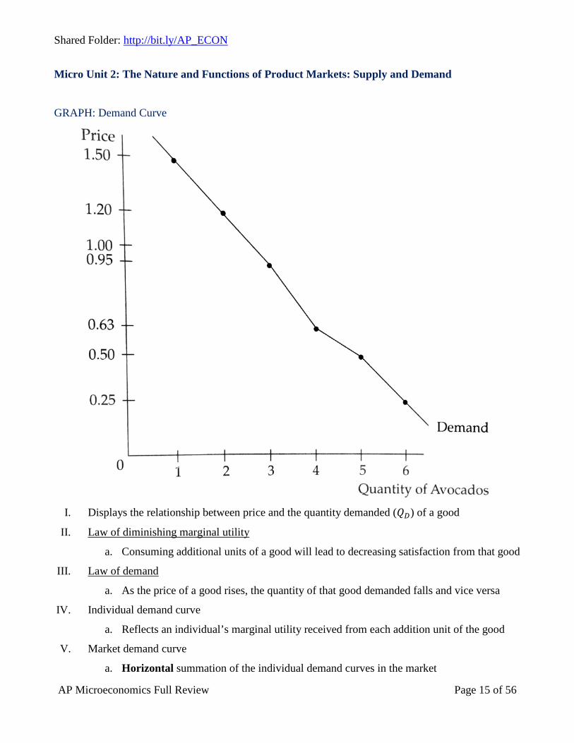
GRAPH: Demand Curve

I. Displays the relationship between price and the quantity demanded (𝑄𝑄𝐷𝐷) of a good

II. Law of diminishing marginal utility

a. Consuming additional units of a good will lead to decreasing satisfaction from that good

III. Law of demand

a. As the price of a good rises, the quantity of that good demanded falls and vice versa

IV. Individual demand curve

a. Reflects an individual’s marginal utility received from each addition unit of the good

V. Market demand curve

a. Horizontal summation of the individual demand curves in the market


VI. Changes in the price of a good only affect the 𝑸𝑸𝑫𝑫 for that good, not the curve itself

VII. Demand shifters to the right (opposite will shift D in)

a. Positive change in tastes or preferences

i. E.g. due to a successful marketing campaign

b. Increase in the price of substitute goods

i. E.g. if the price of peanut butter increases, demand for Nutella will increase

c. Decrease in the price of complements

i. E.g. if the price of jelly decreases, demand for peanut butter will increase

d. Increase in income for normal goods

i. Goods that consumers buys more of when income increases

ii. E.g. higher incomes might lead to increased demand for iPhones

e. Decrease in income for inferior goods

i. Goods that consumers buy more of when income decreases

ii. E.g. lower incomes might lead to increased demand for Spam

f. Increase in the number of buyers in the market

i. More individual demand curves are added to produce the market demand curve

g. Expectations of higher future income

i. Will spend more now

h. Expectations of higher future prices

i. Expectations of future shortages

j. Lower taxes or higher subsidies

EXAMPLE: Summation of Individual Demand Curves



GRAPH: Marginal Utility (MU) vs. Total Utility

I. Marginal utility

a. Additional utility gained from consuming one more unit of a good

b. MU at a particular quantity is the slope of the total utility curve at that quantity

II. Total utility

a. Found by adding the MU values gained from each of the units consumed

III. When MU is positive, total utility is increasing

IV. When MU is zero, total utility is maximized

V. When MU is negative, total utility is decreasing


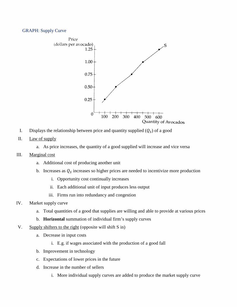
GRAPH: Supply Curve

I. Displays the relationship between price and quantity supplied (𝑄𝑄𝑆𝑆) of a good

II. Law of supply

a. As price increases, the quantity of a good supplied will increase and vice versa

III. Marginal cost

a. Additional cost of producing another unit

b. Increases as 𝑄𝑄𝑆𝑆 increases so higher prices are needed to incentivize more production

i. Opportunity cost continually increases

ii. Each additional unit of input produces less output

iii. Firms run into redundancy and congestion

IV. Market supply curve

a. Total quantities of a good that supplies are willing and able to provide at various prices

b. Horizontal summation of individual firm’s supply curves

V. Supply shifters to the right (opposite will shift S in)

a. Decrease in input costs

i. E.g. if wages associated with the production of a good fall

b. Improvement in technology

c. Expectations of lower prices in the future

d. Increase in the number of sellers

i. More individual supply curves are added to produce the market supply curve



e. Decrease in the price of “substitutes in production” (less common)

i. E.g. if a firm produces both milk and cheese, and the price of milk falls, then more

cheese will be supplied b/c the supplies can make more money off of the cheese

f. Increase in the price of “joint products” (less common)

i. E.g. if a firm produces both leather and beef, and the price of leather increases, then

more cows will be killed and the supply of beef also increases

g. Lower taxes or higher subsidies

EXAMPLE: Summation of Individual Supply Curves

GRAPH: Supply and Demand


I. Market equilibrium

a. Point of intersection between the supply and demand curves

b. At the market equilibrium price (𝑃𝑃𝑐𝑐), quantity demanded = quantity supplied

II. Surplus

a. Occurs when price is greater than 𝑃𝑃𝑐𝑐

III. Shortage

a. Occurs when price is lower than 𝑃𝑃𝑐𝑐

EXAMPLE: Supply or Demand Shifting

I. Important to distinguish between movement on the supply/demand curves and actual shifts of the

supply/demand curves

a. Movement along a stationary curve represents a change in 𝑄𝑄𝑆𝑆 or 𝑄𝑄𝐷𝐷

II. When the supply curve shifts from 𝑆𝑆1 𝑐𝑐𝑏𝑏 𝑆𝑆2, market equilibrium moves from 𝐸𝐸1 𝑐𝑐𝑏𝑏 𝐸𝐸2

III. Thus 𝑃𝑃𝑐𝑐 moves from 𝑃𝑃1 𝑐𝑐𝑏𝑏 𝑃𝑃2 and quantity demanded changes from 𝑄𝑄1 𝑐𝑐𝑏𝑏 𝑄𝑄2

a. This is not a shift of the demand curve but rather a shift on the demand curve



EXAMPLE: Supply and Demand Shifting

I. Make sure you are shifting the correct curve(s) when working with these problems

II. Indeterminate

a. When both supply and demand shift, and you don’t know the size of the shifts, either the

resulting 𝑃𝑃𝑐𝑐 𝑏𝑏𝐵𝐵 𝑄𝑄𝑐𝑐 will be indeterminate

GRAPH: Consumer and Producer Surplus

I. Consumer surplus

a. Value received from the purchase in excess of what is paid for it

II. Producer surplus

a. Difference between the price a seller receives and the minimum price for which a seller

would be willing to supply that good


GRAPH: Price Ceilings

I. Non-effective price ceiling

a. Price ceiling is above 𝑃𝑃𝑐𝑐

II. Effective price ceiling

a. Price ceiling is below 𝑃𝑃𝑐𝑐

b. Provide lower costs for consumers

c. Leads to a shortage in the market as 𝑄𝑄𝐷𝐷 > 𝑄𝑄𝑆𝑆

d. Can also result in illegal black market activity

i. Sell goods for a higher price than the price ceiling

GRAPH: Price Floors



I. Non-effective price floor

a. Price floor is below 𝑃𝑃𝑐𝑐

II. Effective price floor

a. Price ceiling is above 𝑃𝑃𝑐𝑐

i. E.g. minimum wage

b. Leads to a surplus in the market as 𝑄𝑄𝑆𝑆 > 𝑄𝑄𝐷𝐷

EXAMPLE: Tax on Buyers (Demand)

I. Graph represents a tax on the use of hotel rooms, which is imposed on guests

II. Tax = vertical distance between the two demand curves

a. Burden of the tax does not depend on who has to pay for it

b. Burden of the tax depends on the relative elasticities of the supply and demand curves

i. More elastic curve is burdened by a larger portion of the tax

ii. Perfectly inelastic supply curve would place the entire burden of the tax on supplies

iii. Perfectly inelastic demand curve would place the entire burden of the tax on buyers

III. Deadweight loss (DWL)

a. Represents the loss to former consumer and producer surplus in excess of the total revenue

of the tax: transactions that would have taken place in the market if there was no tax


IV. Without the tax

a. Demand = 𝐷𝐷1

b. Supply = 𝑆𝑆1

c. 𝑃𝑃𝑐𝑐 = 75

d. Consumer surplus = ACG

e. Producer surplus = GCE

V. With the tax

a. Demand = 𝐷𝐷𝑇𝑇

b. Supply = 𝑆𝑆1

c. 𝑃𝑃 = 𝑃𝑃𝑐𝑐 + 𝑐𝑐𝐵𝐵𝑀𝑀 = $71 + $10 = $81

i. Price consumers have to pay has increased by $6, from $75 to $81

ii. Price supplies receive has decreased by $4, from $75 to $71

d. Consumer surplus = ABH

e. Producer surplus = FDE

f. Tax revenue = tax amount × quantity = $10 × 94 = $940

g. DWL = BCD

EXAMPLE: Tax on Suppliers (Supply)

I. Graph represents a tax on the use of hotel rooms, which is imposed on the hotels

II. Same result as a $10 tax on hotel guests

III. See “EXAMPLE: Tax on Buyers (Demand)” for more info on taxes



Micro Unit 3: Production, Costs, and Elasticity

Elasticity

I. Measure of how responsive something is to various changes

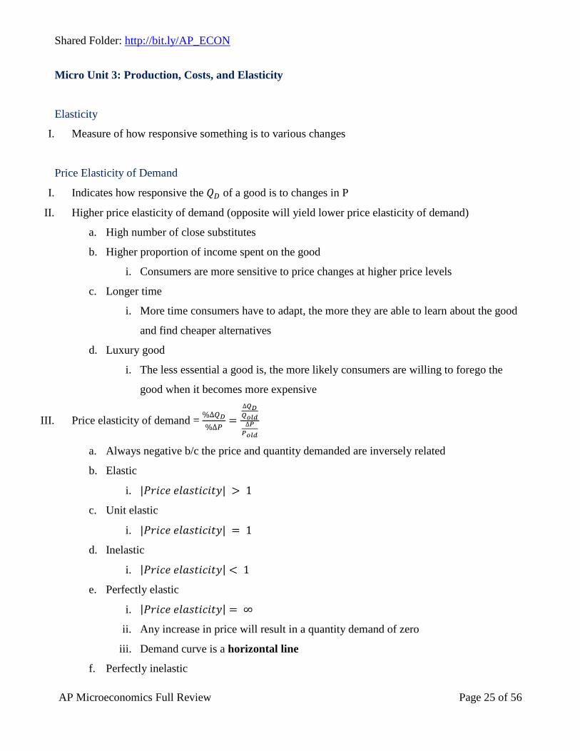
Price Elasticity of Demand

I. Indicates how responsive the 𝑄𝑄𝐷𝐷 of a good is to changes in P

II. Higher price elasticity of demand (opposite will yield lower price elasticity of demand)

a. High number of close substitutes

b. Higher proportion of income spent on the good

i. Consumers are more sensitive to price changes at higher price levels

c. Longer time

i. More time consumers have to adapt, the more they are able to learn about the good

and find cheaper alternatives

d. Luxury good

i. The less essential a good is, the more likely consumers are willing to forego the

good when it becomes more expensive

III. Price elasticity of demand = %∆𝑄𝑄𝐷𝐷%∆𝑃𝑃

=∆𝑄𝑄𝐷𝐷𝑄𝑄𝑓𝑓𝑐𝑐𝑓𝑓∆𝑃𝑃𝑃𝑃𝑓𝑓𝑐𝑐𝑓𝑓

a. Always negative b/c the price and quantity demanded are inversely related

b. Elastic

i. |𝑃𝑃𝐵𝐵𝐵𝐵𝑏𝑏𝑐𝑐 𝑐𝑐𝐵𝐵𝐵𝐵𝑏𝑏𝑐𝑐𝐵𝐵𝑏𝑏𝐵𝐵𝑐𝑐𝑢𝑢| > 1

c. Unit elastic

i. |𝑃𝑃𝐵𝐵𝐵𝐵𝑏𝑏𝑐𝑐 𝑐𝑐𝐵𝐵𝐵𝐵𝑏𝑏𝑐𝑐𝐵𝐵𝑏𝑏𝐵𝐵𝑐𝑐𝑢𝑢| = 1

d. Inelastic

i. |𝑃𝑃𝐵𝐵𝐵𝐵𝑏𝑏𝑐𝑐 𝑐𝑐𝐵𝐵𝐵𝐵𝑏𝑏𝑐𝑐𝐵𝐵𝑏𝑏𝐵𝐵𝑐𝑐𝑢𝑢| < 1

e. Perfectly elastic

i. |𝑃𝑃𝐵𝐵𝐵𝐵𝑏𝑏𝑐𝑐 𝑐𝑐𝐵𝐵𝐵𝐵𝑏𝑏𝑐𝑐𝐵𝐵𝑏𝑏𝐵𝐵𝑐𝑐𝑢𝑢| = ∞

ii. Any increase in price will result in a quantity demand of zero

iii. Demand curve is a horizontal line

f. Perfectly inelastic


i. |𝑃𝑃𝐵𝐵𝐵𝐵𝑏𝑏𝑐𝑐 𝑐𝑐𝐵𝐵𝐵𝐵𝑏𝑏𝑐𝑐𝐵𝐵𝑏𝑏𝐵𝐵𝑐𝑐𝑢𝑢| = 0

ii. Price has no influence on quantity demanded

iii. Demand curve is a vertical line

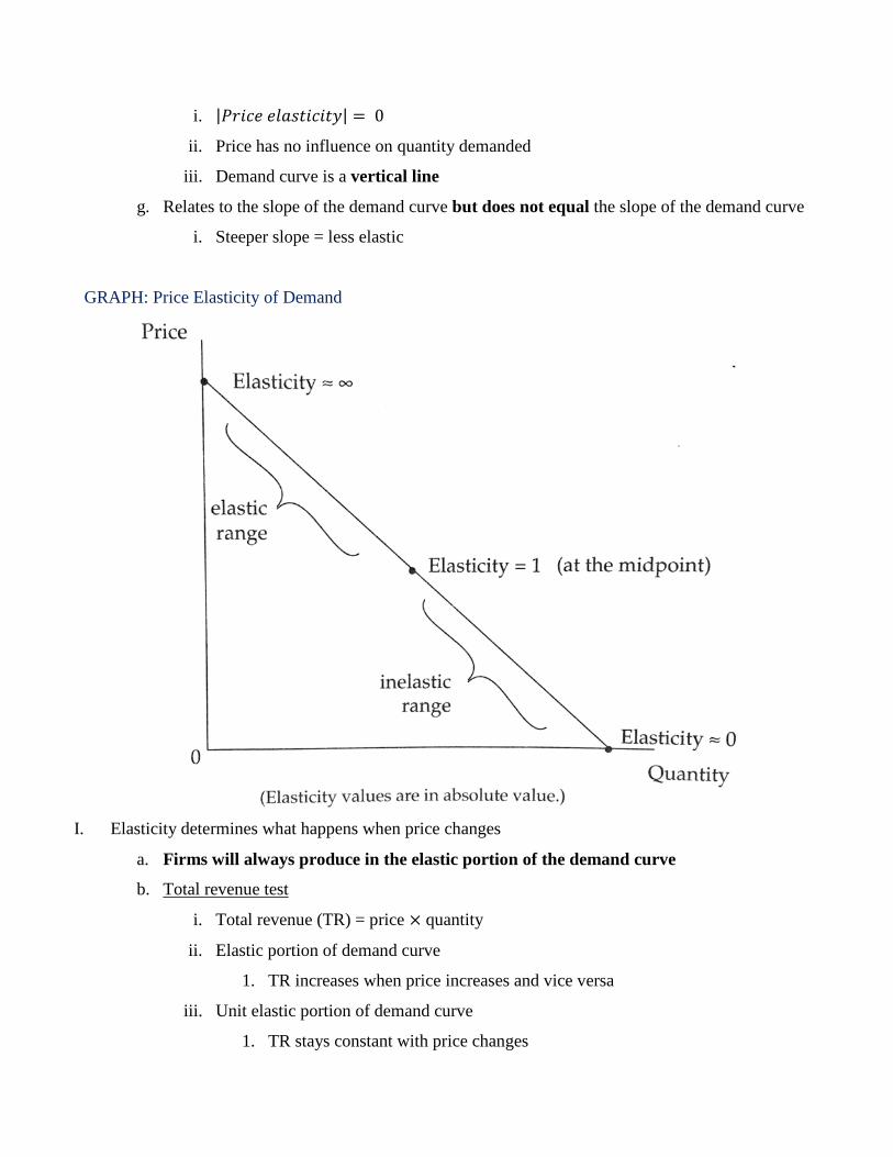
g. Relates to the slope of the demand curve but does not equal the slope of the demand curve

i. Steeper slope = less elastic

GRAPH: Price Elasticity of Demand

I. Elasticity determines what happens when price changes

a. Firms will always produce in the elastic portion of the demand curve

b. Total revenue test

i. Total revenue (TR) = price × quantity

ii. Elastic portion of demand curve

1. TR increases when price increases and vice versa

iii. Unit elastic portion of demand curve

1. TR stays constant with price changes



iv. Inelastic portion of demand curve

1. TR decrease when price increases and vice versa

II. As we move left to right along a demand curve, the elasticity will go from negative infinity to zero2

EXAMPLE: Total Revenue Test

Price Elasticity of Supply

I. Indicates how responsive the 𝑄𝑄𝑆𝑆 of a good is to changes in P

II. Price elasticity of demand = %∆𝑄𝑄𝑆𝑆%∆𝑃𝑃

=∆𝑄𝑄𝑆𝑆𝑄𝑄𝑓𝑓𝑐𝑐𝑓𝑓∆𝑃𝑃𝑃𝑃𝑓𝑓𝑐𝑐𝑓𝑓

a. Always positive b/c the price and quantity supplied are directly related

b. Elastic

i. 𝑃𝑃𝐵𝐵𝐵𝐵𝑏𝑏𝑐𝑐 𝑐𝑐𝐵𝐵𝐵𝐵𝑏𝑏𝑐𝑐𝐵𝐵𝑏𝑏𝐵𝐵𝑐𝑐𝑢𝑢 > 1

c. Unit elastic

i. 𝑃𝑃𝐵𝐵𝐵𝐵𝑏𝑏𝑐𝑐 𝑐𝑐𝐵𝐵𝐵𝐵𝑏𝑏𝑐𝑐𝐵𝐵𝑏𝑏𝐵𝐵𝑐𝑐𝑢𝑢 = 1

d. Inelastic

i. 𝑃𝑃𝐵𝐵𝐵𝐵𝑏𝑏𝑐𝑐 𝑐𝑐𝐵𝐵𝐵𝐵𝑏𝑏𝑐𝑐𝐵𝐵𝑏𝑏𝐵𝐵𝑐𝑐𝑢𝑢 < 1

e. Perfectly elastic

i. 𝑃𝑃𝐵𝐵𝐵𝐵𝑏𝑏𝑐𝑐 𝑐𝑐𝐵𝐵𝐵𝐵𝑏𝑏𝑐𝑐𝐵𝐵𝑏𝑏𝐵𝐵𝑐𝑐𝑢𝑢 = ∞

ii. Any decrease in price will result in a quantity supplied of zero

2 For this particular graph, the given elasticity values are in absolute value.


iii. Supply curve is a horizontal line

f. Perfectly inelastic

i. 𝑃𝑃𝐵𝐵𝐵𝐵𝑏𝑏𝑐𝑐 𝑐𝑐𝐵𝐵𝐵𝐵𝑏𝑏𝑐𝑐𝐵𝐵𝑏𝑏𝐵𝐵𝑐𝑐𝑢𝑢 = 0

ii. Price has no influence on quantity supplied

iii. Supply curve is a vertical line

g. Relates to the slope of the supply curve but does not equal the slope of the demand curve

i. Steeper slope = less elastic

Income Elasticity of Demand

I. Indicates how responsive the 𝑄𝑄𝐷𝐷 of a good is to changes in income

II. Income elasticity of demand= %∆𝑄𝑄𝐷𝐷%∆𝐼𝐼

=∆𝑄𝑄𝐷𝐷𝑄𝑄𝑓𝑓𝑐𝑐𝑓𝑓∆𝐼𝐼𝐼𝐼𝑓𝑓𝑐𝑐𝑓𝑓

a. Normal good

i. Individual purchases more of when income increases

ii. 𝑃𝑃𝐵𝐵𝐵𝐵𝑏𝑏𝑐𝑐 𝑐𝑐𝐵𝐵𝐵𝐵𝑏𝑏𝑐𝑐𝐵𝐵𝑏𝑏𝐵𝐵𝑐𝑐𝑢𝑢 > 1

b. Inferior good

i. Individual purchases more of when income decreases

ii. 𝑃𝑃𝐵𝐵𝐵𝐵𝑏𝑏𝑐𝑐 𝑐𝑐𝐵𝐵𝐵𝐵𝑏𝑏𝑐𝑐𝐵𝐵𝑏𝑏𝐵𝐵𝑐𝑐𝑢𝑢 < 1

Cross-Price Elasticity of Demand

I. Indicates how responsive the 𝑄𝑄𝐷𝐷 of a good is to changes in P of another good

II. Cross-price elasticity of demand = %∆𝑄𝑄𝐷𝐷 𝑓𝑓𝑓𝑓 𝐺𝐺𝑓𝑓𝑓𝑓𝑓𝑓 𝐴𝐴

%∆𝑃𝑃𝐺𝐺𝑓𝑓𝑓𝑓𝑓𝑓 𝐵𝐵=

∆𝑄𝑄𝐷𝐷 𝑓𝑓𝑓𝑓 𝐺𝐺𝑓𝑓𝑓𝑓𝑓𝑓 𝐴𝐴𝑄𝑄𝑓𝑓𝑐𝑐𝑓𝑓 𝑓𝑓𝑓𝑓 𝐺𝐺𝑓𝑓𝑓𝑓𝑓𝑓 𝐴𝐴

∆𝑃𝑃𝐺𝐺𝑓𝑓𝑓𝑓𝑓𝑓 𝐵𝐵𝑃𝑃𝑓𝑓𝑐𝑐𝑓𝑓 𝑓𝑓𝑓𝑓 𝐺𝐺𝑓𝑓𝑓𝑓𝑓𝑓 𝐵𝐵

a. Substitutes

i. Individual purchases less of when the price of another good increases

ii. 𝐶𝐶𝐵𝐵𝑏𝑏𝑏𝑏𝑏𝑏 𝑐𝑐𝐵𝐵𝐵𝐵𝑏𝑏𝑐𝑐 𝑐𝑐𝐵𝐵𝐵𝐵𝑏𝑏𝑐𝑐𝐵𝐵𝑏𝑏𝐵𝐵𝑐𝑐𝑢𝑢 > 1

b. Complements

i. Individual purchases more of when price of another good decreases

ii. 𝐶𝐶𝐵𝐵𝑏𝑏𝑏𝑏𝑏𝑏 𝑐𝑐𝐵𝐵𝐵𝐵𝑏𝑏𝑐𝑐 𝑐𝑐𝐵𝐵𝐵𝐵𝑏𝑏𝑐𝑐𝐵𝐵𝑏𝑏𝐵𝐵𝑐𝑐𝑢𝑢 < 1



GRAPH: Marginal Product and Total Product

I. Marginal product (𝑀𝑀𝑃𝑃) = ∆𝑜𝑜𝑜𝑜𝑜𝑜𝑡𝑡𝑏𝑏 𝑜𝑜𝑜𝑜𝑜𝑜𝑝𝑝𝑜𝑜𝑐𝑐𝑜𝑜∆𝑜𝑜𝑜𝑜𝑜𝑜𝑜𝑜𝑜𝑜

a. Additional output produced per when one more unit of an input is added, ceteris paribus

b. Sometimes called the marginal physical product

i. Reminder that dollars aren’t involved: just a measure of physical output

c. Increases with the first few workers as they are able to take advantage of specialization

II. Law of diminishing marginal returns

a. As the amount of one input is increased, incremental gains in output, or marginal returns,

will eventually decrease, ceteris paribus

b. E.g. consider hiring more workers, eventually too many workers leads to boredom and the

distraction of other workers

III. Average product (𝐴𝐴𝑃𝑃) = 𝑜𝑜𝑜𝑜𝑜𝑜𝑡𝑡𝑏𝑏 𝑜𝑜𝑜𝑜𝑜𝑜𝑝𝑝𝑜𝑜𝑐𝑐𝑜𝑜𝑞𝑞𝑜𝑜𝑡𝑡𝑜𝑜𝑜𝑜𝑜𝑜𝑜𝑜𝑜𝑜 𝑜𝑜𝑓𝑓 𝑜𝑜𝑜𝑜𝑜𝑜𝑜𝑜𝑜𝑜


a. Rises when MP is above it and falls when MP is below it

i. Think of the MP curve as your score on each new AP economics test, and the AP

curve as your average grade in AP economics

b. Reaches its maximum when it intersects the MP curve

IV. Total product curve

a. Shows the relationship between the total amount of output produced and number of units of

an input used, ceteris paribus

b. Slope = marginal product

c. Rises when MP is positive and vice versa

d. Remains constant when MP is zero

GRAPH: Marginal Cost and Total Cost



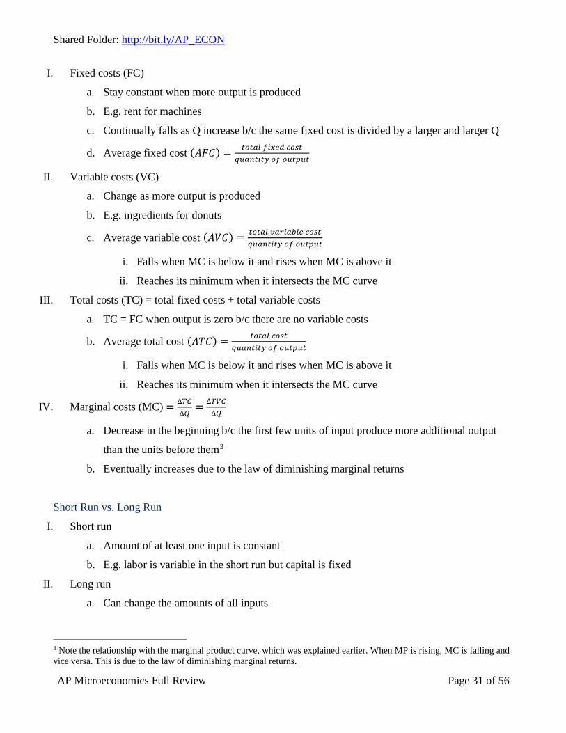
I. Fixed costs (FC)

a. Stay constant when more output is produced

b. E.g. rent for machines

c. Continually falls as Q increase b/c the same fixed cost is divided by a larger and larger Q

d. Average fixed cost (𝐴𝐴𝐴𝐴𝐶𝐶) = 𝑜𝑜𝑜𝑜𝑜𝑜𝑡𝑡𝑏𝑏 𝑓𝑓𝑜𝑜𝑓𝑓𝑐𝑐𝑝𝑝 𝑐𝑐𝑜𝑜𝑐𝑐𝑜𝑜𝑞𝑞𝑜𝑜𝑡𝑡𝑜𝑜𝑜𝑜𝑜𝑜𝑜𝑜𝑜𝑜 𝑜𝑜𝑓𝑓 𝑜𝑜𝑜𝑜𝑜𝑜𝑜𝑜𝑜𝑜𝑜𝑜

II. Variable costs (VC)

a. Change as more output is produced

b. E.g. ingredients for donuts

c. Average variable cost (𝐴𝐴𝐴𝐴𝐶𝐶) = 𝑜𝑜𝑜𝑜𝑜𝑜𝑡𝑡𝑏𝑏 𝑣𝑣𝑡𝑡𝑜𝑜𝑜𝑜𝑡𝑡𝑏𝑏𝑏𝑏𝑐𝑐 𝑐𝑐𝑜𝑜𝑐𝑐𝑜𝑜𝑞𝑞𝑜𝑜𝑡𝑡𝑜𝑜𝑜𝑜𝑜𝑜𝑜𝑜𝑜𝑜 𝑜𝑜𝑓𝑓 𝑜𝑜𝑜𝑜𝑜𝑜𝑜𝑜𝑜𝑜𝑜𝑜

i. Falls when MC is below it and rises when MC is above it

ii. Reaches its minimum when it intersects the MC curve

III. Total costs (TC) = total fixed costs + total variable costs

a. TC = FC when output is zero b/c there are no variable costs

b. Average total cost (𝐴𝐴𝐴𝐴𝐶𝐶) = 𝑜𝑜𝑜𝑜𝑜𝑜𝑡𝑡𝑏𝑏 𝑐𝑐𝑜𝑜𝑐𝑐𝑜𝑜𝑞𝑞𝑜𝑜𝑡𝑡𝑜𝑜𝑜𝑜𝑜𝑜𝑜𝑜𝑜𝑜 𝑜𝑜𝑓𝑓 𝑜𝑜𝑜𝑜𝑜𝑜𝑜𝑜𝑜𝑜𝑜𝑜

i. Falls when MC is below it and rises when MC is above it

ii. Reaches its minimum when it intersects the MC curve

IV. Marginal costs (MC) = ∆𝑇𝑇𝑇𝑇∆𝑄𝑄

= ∆𝑇𝑇𝑇𝑇𝑇𝑇∆𝑄𝑄

a. Decrease in the beginning b/c the first few units of input produce more additional output

than the units before them3

b. Eventually increases due to the law of diminishing marginal returns

Short Run vs. Long Run

I. Short run

a. Amount of at least one input is constant

b. E.g. labor is variable in the short run but capital is fixed

II. Long run

a. Can change the amounts of all inputs

3 Note the relationship with the marginal product curve, which was explained earlier. When MP is rising, MC is falling and vice versa. This is due to the law of diminishing marginal returns.


i. No fixed costs

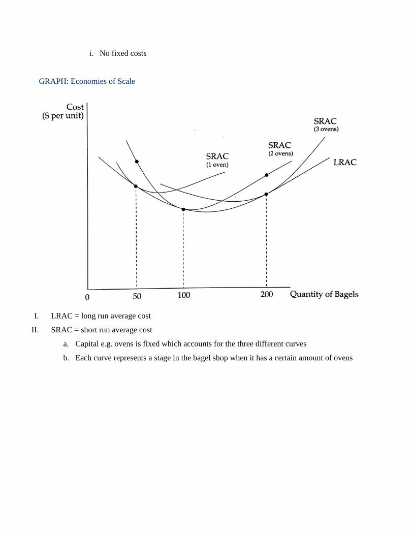
GRAPH: Economies of Scale

I. LRAC = long run average cost

II. SRAC = short run average cost

a. Capital e.g. ovens is fixed which accounts for the three different curves

b. Each curve represents a stage in the bagel shop when it has a certain amount of ovens



Micro Unit 4: Perfect Competition

Key Terms

I. Economies of scale

a. Occur during the range of output where LRAC slopes downward

b. Can result from increasing returns to scale

II. Diseconomies of scale

a. Occur during the range of output where LRAC slopes upward

III. Increasing returns to scale

a. Output increases proportionally more than increases in all inputs

i. E.g. doubling all inputs yields three times the amount of output

b. Often confused with increasing marginal returns

i. Only involved an increase in one input, ceteris paribus

IV. Decreasing returns to scale

a. Output increases proportionally less than increase in all inputs

i. E.g. doubling all inputs yields 1.5 times the amount of output

V. Constant returns to scale

a. Output increase proportionally to increases in all inputs

i. E.g. doubling all inputs yields two times the amount of output

VI. Productive efficiency

a. P = minimum ATC

VII. Allocation efficiency

a. P = MC

VIII. Increasing cost firm (less common)

a. Firm facing decreasing returns to scale

IX. Decreasing cost firm (less common)

a. Firm facing increasing returns to scale

X. Increasing cost industry (less common)

a. Experiences increases in average production costs as industry output increases

b. More likely to occur in large industries where input prices increases with higher demand

i. E.g. automobiles


c. Upward sloping long run supply curve

XI. Decreasing cost industry (less common)

a. Experiences decreases in average production costs as industry output increases

b. More likely to occur in industries where production is only possible at a mass level

i. E.g. solar panels

c. Downward sloping long run supply curve

XII. Constant cost industry (less common)

a. Does not experience changes in production costs as industry output increases

b. Horizontal sloping long run supply curve

EXAMPLE: Decreasing Cost Industry (less common)

I. Short run


b. Price = 𝑃𝑃1

c. Supply = 𝑆𝑆1

d. Firm quantity = 𝑞𝑞1

e. Market quantity = 𝑄𝑄1

II. Long run


i. Suppose there is an increase in demand

b. Price = 𝑃𝑃2 → 𝑃𝑃3

i. Price initially rises to 𝑃𝑃2



1. At this price, firms are earning an economic profit

2. Availability of profits will draw new firms, causing supply to shift out

ii. B/c this is a decreasing costs industry, even when price returns to 𝑃𝑃1 (due to the

supply curve shifting out), firms are still making economic profit as their costs will

be lower than in the beginning when 𝑃𝑃1 corresponded to zero economic profit

iii. Supply curve will continue to shift out until falling prices correspond to falling

average and marginal costs, and thus zero economic profit earned by firms

c. Supply = 𝑆𝑆2

d. Firm quantity = 𝑞𝑞2 → 𝑞𝑞3

i. Firm quantity initially rises to 𝑞𝑞2 but then falls to 𝑞𝑞3

e. Market quantity = 𝑄𝑄2 → 𝑄𝑄3

i. Market quantity initially rises to 𝑄𝑄2 and then increases even more to 𝑄𝑄3

GRAPH: Perfect Competition

I. Key characteristics

a. Many sellers

i. E.g. agricultural goods

b. Homogeneous, or identical, products

c. Firms are price takers

d. Free entry and exit from market

e. Zero economic profits in long run

i. Firms will enter the market to compete away existing profits

ii. Firms will leave the market to eliminate any losses


II. Mr. DARP4

a. Marginal revenue = firm demand curve = average revenue = market price

b. 𝑀𝑀𝑀𝑀 = ∆𝑇𝑇𝑇𝑇∆𝑄𝑄

c. 𝐴𝐴𝑀𝑀 = 𝑇𝑇𝑇𝑇𝑄𝑄

III. Market S and D curves are the horizontal summations of individual firm’s S and Demand curves5

IV. Economic profit6 = total revenues – total costs

a. Implicit costs i.e. opportunity costs are included in total costs

b. Zero economic profit = you couldn’t be making any more money doing anything different

c. Normal profit = zero economic profit

V. Accounting profit = total revenues – explicit costs

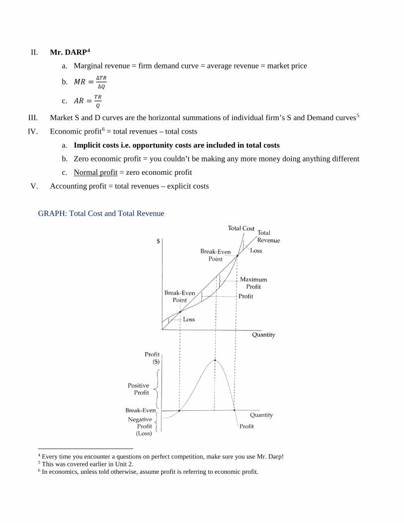
GRAPH: Total Cost and Total Revenue

4 Every time you encounter a questions on perfect competition, make sure you use Mr. Darp! 5 This was covered earlier in Unit 2. 6 In economics, unless told otherwise, assume profit is referring to economic profit.



I. When TR is greater than TC, vertical distance represents profits

II. When TR is less than TC, vertical distance represents losses

III. Firms want to produce where profit is maximized

a. MR = MC

i. In other words: slope of the TR curve = slope of the total cost curve

GRAPH: Perfect Competition – Profit Maximizing Firm7

I. Total profit is positive when P > ATC

a. In this graph, total profit = TR – TC = ABFE – DCFE = ABCD

II. Total profit is negative when P < ATC

III. Total profit is zero when P = ATC

7 AC is the same thing as ATC. The corresponding market graph is not shown to the right.


GRAPH: Shut Down Decision

I. Short run: depends on whether or not P exceeds AVC

II. Long run: depends on whether or not P exceeds ATC

III. P > ATC

a. Firm is making economic profits

IV. AVC < P < ATC

a. Firm is incurring economic losses but will stay open

b. Two options in the short run

i. Shut down and not incur variable costs, but not obtain any revenue for fixed costs

ii. Remain open and cover all of its variable costs (b/c P > AVC), and pay off some of

its fixed costs with the difference between P and AVC

1. Better of the two alternatives

V. P < AVC

a. Firm is incurring economic losses and will shut down as it can’t cover its variable costs



Micro Unit 5: Monopolies

GRAPH: Monopoly


a. Sole provider of a unique product8

i. E.g. local monopolies such as a the sole movie theater in a small town

b. Absolute monopolies are rare at the national and international level

c. Barriers to entry allow economic profits in the long run

i. Patents

ii. Control of resources

1. E.g. diamond mines

iii. Exclusive licenses

1. E.g. gov. grants only one company the right to produce electricity

II. Demand curve is downward sloping

8 Just because they are the sole provider of the product, it doesn’t mean that monopolies can charge whatever price they want. Consumers will not buy a product if the price is higher than the demand curve.


a. Lower price must be charged on all previous units to sell additional units

b. Price ≠ marginal revenue at output levels greater than zero

i. MR falls as Q increases

III. Always produces in the elastic portion of the demand curve when maximizing profits

a. Find where MR = MC to find the quantity of output

b. Trace your finger upwards until you hit the demand curve to find price

IV. Monopolies produce less and at a higher price than firms in perfect competition

Price Discrimination

I. E.g. airlines, car dealers, Uber

II. Key characteristics

a. Firm must have market power: downward sloping demand curve

b. Buyers with differing demand elasticities must be separable

c. Firm must be able to prevent the resale of its goods

i. Block those paying the lower price to resell to those willing to pay the higher price

III. Want to charge customers the most they are willing to pay

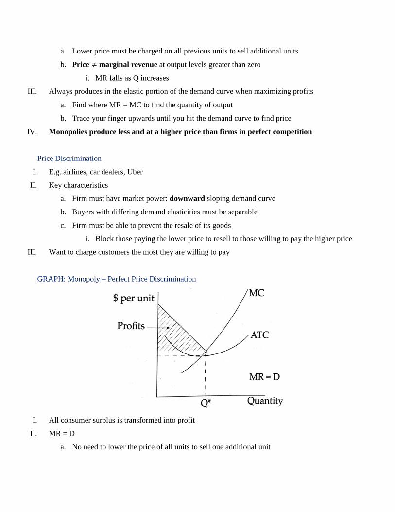
GRAPH: Monopoly – Perfect Price Discrimination

I. All consumer surplus is transformed into profit

II. MR = D

a. No need to lower the price of all units to sell one additional unit



GRAPH: Monopoly – Perfect Price Discrimination w/Differing Demand Elasticities

I. The more inelastic the demand, the more consumers pay

EXAMPLE: Government Policy towards Imperfect Competition


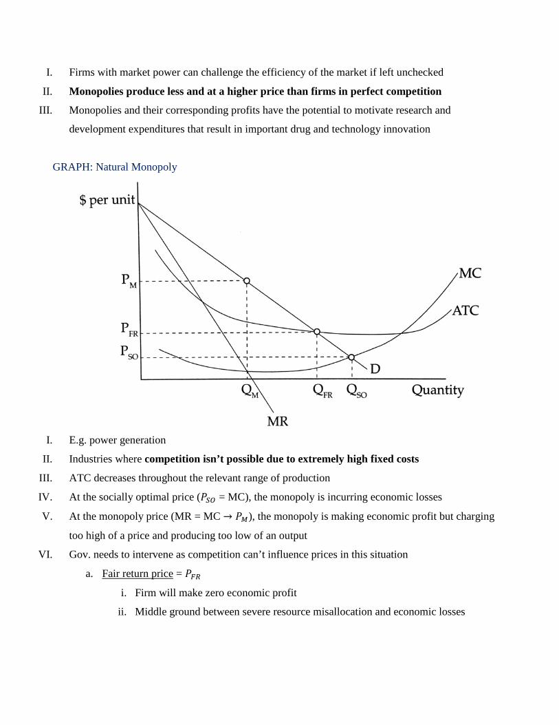
I. Firms with market power can challenge the efficiency of the market if left unchecked

II. Monopolies produce less and at a higher price than firms in perfect competition

III. Monopolies and their corresponding profits have the potential to motivate research and

development expenditures that result in important drug and technology innovation

GRAPH: Natural Monopoly

I. E.g. power generation

II. Industries where competition isn’t possible due to extremely high fixed costs

III. ATC decreases throughout the relevant range of production

IV. At the socially optimal price (𝑃𝑃𝑆𝑆𝑆𝑆 = MC), the monopoly is incurring economic losses

V. At the monopoly price (MR = MC → 𝑃𝑃𝑀𝑀), the monopoly is making economic profit but charging

too high of a price and producing too low of an output

VI. Gov. needs to intervene as competition can’t influence prices in this situation

a. Fair return price = 𝑃𝑃𝐹𝐹𝑇𝑇

i. Firm will make zero economic profit

ii. Middle ground between severe resource misallocation and economic losses



Micro Unit 6: Monopolistic Competition and Oligopolies

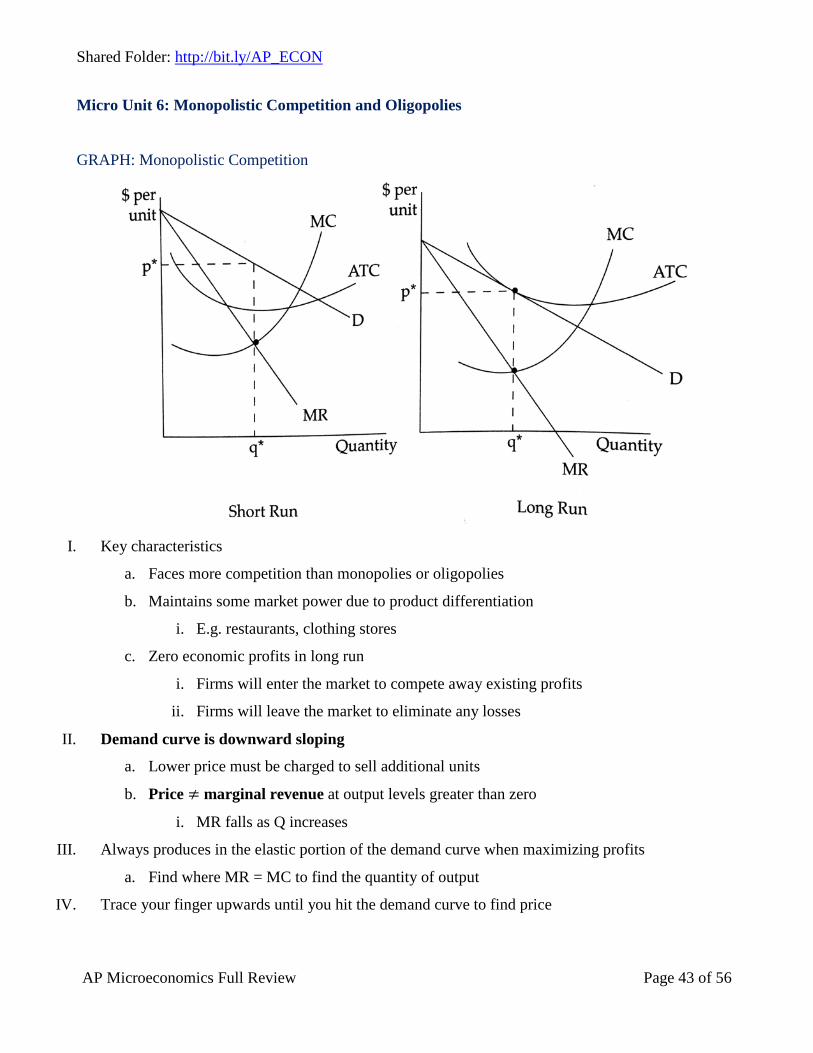
GRAPH: Monopolistic Competition


a. Faces more competition than monopolies or oligopolies

b. Maintains some market power due to product differentiation

i. E.g. restaurants, clothing stores

c. Zero economic profits in long run

i. Firms will enter the market to compete away existing profits

ii. Firms will leave the market to eliminate any losses

II. Demand curve is downward sloping

a. Lower price must be charged to sell additional units

b. Price ≠ marginal revenue at output levels greater than zero

i. MR falls as Q increases

III. Always produces in the elastic portion of the demand curve when maximizing profits

a. Find where MR = MC to find the quantity of output

IV. Trace your finger upwards until you hit the demand curve to find price


Oligopoly

I. E.g. airlines, Coca-Cola vs. Pepsi


a. Small number of firms selling a homogeneous or differentiated product

b. High barriers to entry and high market power

c. Mutualistic interdependence

i. Decision of one firm will highly impact the decisions of other firms

Game Theory

I. Considers the strategic decision of players (e.g. interdependent ogopolistic firms) in anticipation of

their competitors’ reactions

II. Payoff matrix: two by two square

a. Details the possible results of varying pricing choices by two entities

b. Isolate one player and one strategy and circle the best choice for the other player

i. It can be helpful to cover up the other side of the square

ii. E.g. use circles for player 1 and rectangles for player 2 for their best choices

III. Dominant strategy

a. Choosing one pricing strategy regardless of what the competitor chooses

IV. Nash equilibrium9

a. Occurs when two choices appear in the same square of a payoff matrix

b. Dominant strategy equilibrium

i. Both sides have a dominant strategy, so neither party will deviate from its strategy

given the strategy of the other side

ii. All dominant strategy equilibriums are Nash equilibriums, but not vice versa

V. Prisoner’s dilemma

a. When competing parties forgo an option more beneficial for both parties e.g. Party A and B

choose to make $100 and $200 instead of $300 and $500, respectively

b. E.g. arms races

i. Both parties are better off with peace

9 Rest in peace, John Nash.



EXAMPLE: Payoff Matrix – Dominant Strategy Equilibrium

I. Bob chooses high priced strategy

a. Liz makes 300 going high or makes 500 going low

II. Bob chooses low priced strategy

a. Liz loses 800 going high or loses 500 going low

III. Liz chooses high priced strategy

a. Bob makes 400 going high or makes 600 going low

IV. Liz chooses low priced strategy

a. Bob loses 800 going high or loses 500 going low

V. Nash equilibrium

a. Both players have a dominant strategy of going low

b. Bob ends up losing 500 and Liz ends up losing 500

i. This illustrates the prisoner’s dilemma

1. Both players would have been better off going high


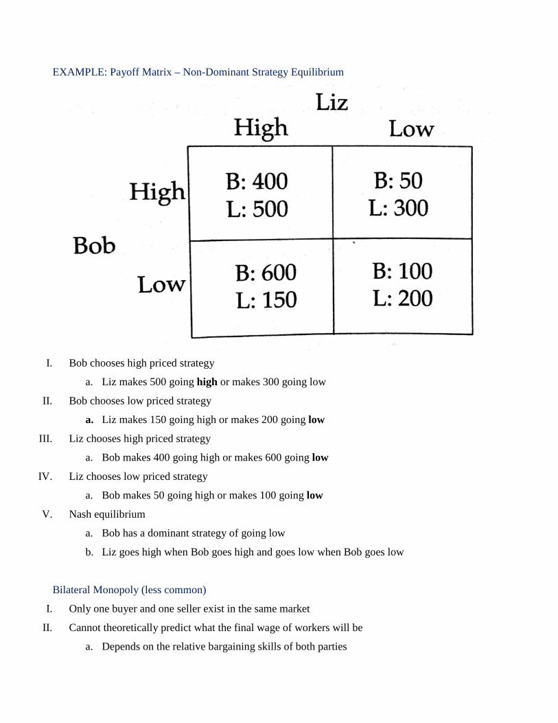
EXAMPLE: Payoff Matrix – Non-Dominant Strategy Equilibrium

I. Bob chooses high priced strategy


II. Bob chooses low priced strategy


III. Liz chooses high priced strategy


IV. Liz chooses low priced strategy


V. Nash equilibrium

a. Bob has a dominant strategy of going low

b. Liz goes high when Bob goes high and goes low when Bob goes low

Bilateral Monopoly (less common)

I. Only one buyer and one seller exist in the same market

II. Cannot theoretically predict what the final wage of workers will be

a. Depends on the relative bargaining skills of both parties



SUMMARY: Market Structures

I. Maximizing profits (without price discrimination) for all market structures

a. Find where MR = MC

b. Go straight down to the x-axis to determine the quantity produced

c. Go straight up to the demand curve to determine the price

i. If the D = MR, this step is easy

d. If price is less than AVC, the firm will shut down

e. Otherwise, the firm will produce at Q and at a price of P

f. Profit = total revenue – total costs = (𝑃𝑃 − 𝐴𝐴𝐴𝐴𝐶𝐶) × 𝑄𝑄


Micro Unit 7: Factor Markets10

Instead of working with demand for products, we are now working with demand for the factors of

production e.g. land, labor, capital. 11

EXAMPLE: Factor Markets – Ice Cream Machines

I. If the demand for ice cream increase, the demand for ice cream machines will also increase

GRAPH: Marginal Revenue Product of Labor

10 This is one of the hardest units in microeconomics. It is easy to confuse product markets with labor markets and vice versa, but you need an adept understanding of both to score well on the AP Test. 11 Most graphs and examples will use labor in the explanation of factor markets. The determination of other factor prices is analogous to the material in this section.



I. 𝑀𝑀𝑀𝑀𝑃𝑃𝐿𝐿 = 𝑀𝑀𝑃𝑃𝐿𝐿 × 𝑃𝑃𝑜𝑜𝑜𝑜𝑜𝑜𝑜𝑜𝑜𝑜𝑜𝑜

II. Assuming firms can’t price discriminate, those facing downward sloping demand curves must

lower the price of all output in order to sell more output produced by additional units of an input

a. The most a firm would be willing to pay for another worker (or other factor of production)

in the short run is that factor of production’s marginal revenue product

III. Want to hire at the intersection of wage and MRP

a. If less workers are hired, there is still the opportunity to hire more workers and pay them

less than the value of their contribution to revenues

b. If more workers are hired, those excess workers are paid more than the value of their

contributions to revenues

IV. If MRP shifts outward, demand for labor will increase and vice versa

V. Demand for labor is a derived demand

a. i.e. firms demand labor b/c consumers demand their products

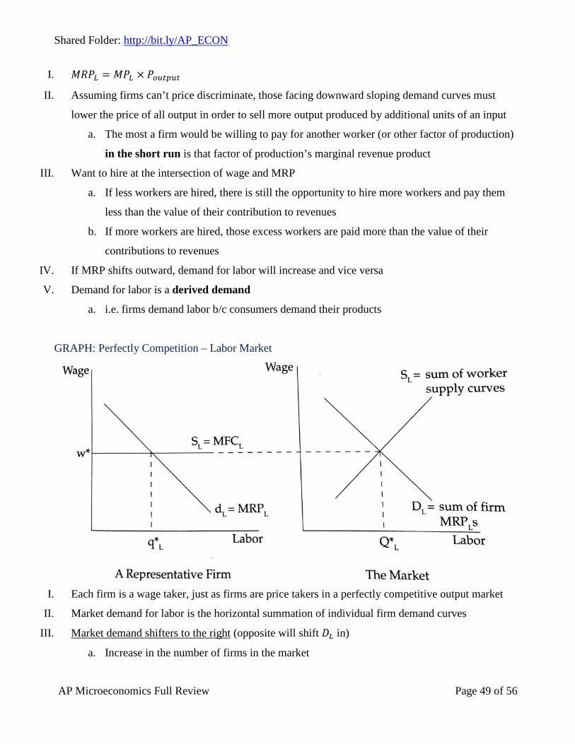
GRAPH: Perfectly Competition – Labor Market

I. Each firm is a wage taker, just as firms are price takers in a perfectly competitive output market

II. Market demand for labor is the horizontal summation of individual firm demand curves

III. Market demand shifters to the right (opposite will shift 𝐷𝐷𝐿𝐿 in)

a. Increase in the number of firms in the market


b. Increase in the 𝑀𝑀𝑀𝑀𝑃𝑃𝐿𝐿 in the individual firms

IV. Equilibrium wage

a. Intersection of 𝑆𝑆𝐿𝐿 and 𝐷𝐷𝐿𝐿

b. Zero unemployment12

i. Everyone who would like to work has the opportunity to do so

GRAPH: Monopsony

I. E.g. mining company in a small mining town

12 Unemployment is discussed further in macroeconomics.




a. Like a monopoly, but for factors of production

III. Supply curve is upward sloping

a. Must raise wages of all workers to hire an additional worker

b. Price ≠ marginal factor cost (MFC) at output levels greater than zero

i. MRC rises as Q increases

IV. Find where MFC = MRP = D to find the quantity of output

a. Trace your finger downwards until you hit the supply curve to find wage

V. In contrast to a perfectly competitive labor market

a. Price = MFC as firms can hire all of the workers they want at the same market wage

b. Firms hire more workers (𝐿𝐿𝑇𝑇) and pay them more (𝑊𝑊𝑐𝑐)

Unions (less common)

I. Workers form unions to increase their collective bargaining and lobbying strengths

II. Goals

a. Increase the demand for labor

b. Decrease the supply of labor

i. Unions comprised of skilled workers do this

c. Negotiate higher wages

i. Unions comprised of unskilled workers tend to use their size to their advantage


Micro Unit 8: Market Failures and the Role of Government

Market Failures

I. Occurs when resources are not allocated efficiency (P = MC)

a. Imperfect competition

b. Externalities

c. Public goods

d. Imperfect information

i. Buyers and sellers don’t have full knowledge about available markets, prices,

products, customers, suppliers, and so forth

ii. E.g. consumers pay too much for a product b/c they aren’t aware of a cheaper

alternative

Externalities

I. Costs and benefits felt beyond those causing the effects: spillover effects

II. Lead to inefficient allocation of resources as those making decisions fail to consider all of the

repercussions of their behavior

III. Negative externalities

a. Lead to overconsumption of a good

b. Solutions

i. Can be taxed by the amount of the MEC

1. E.g. taxing cigarettes

2. Internalize the externality

ii. Restricting output to eh socially optimal quantity

iii. Imposing a price floor at the socially optimal price

IV. Positive externalities

a. Lead to underconsumption of a good

b. Solution

i. Can be subsidized by the amount of the MEB

1. E.g. subsidizing higher education



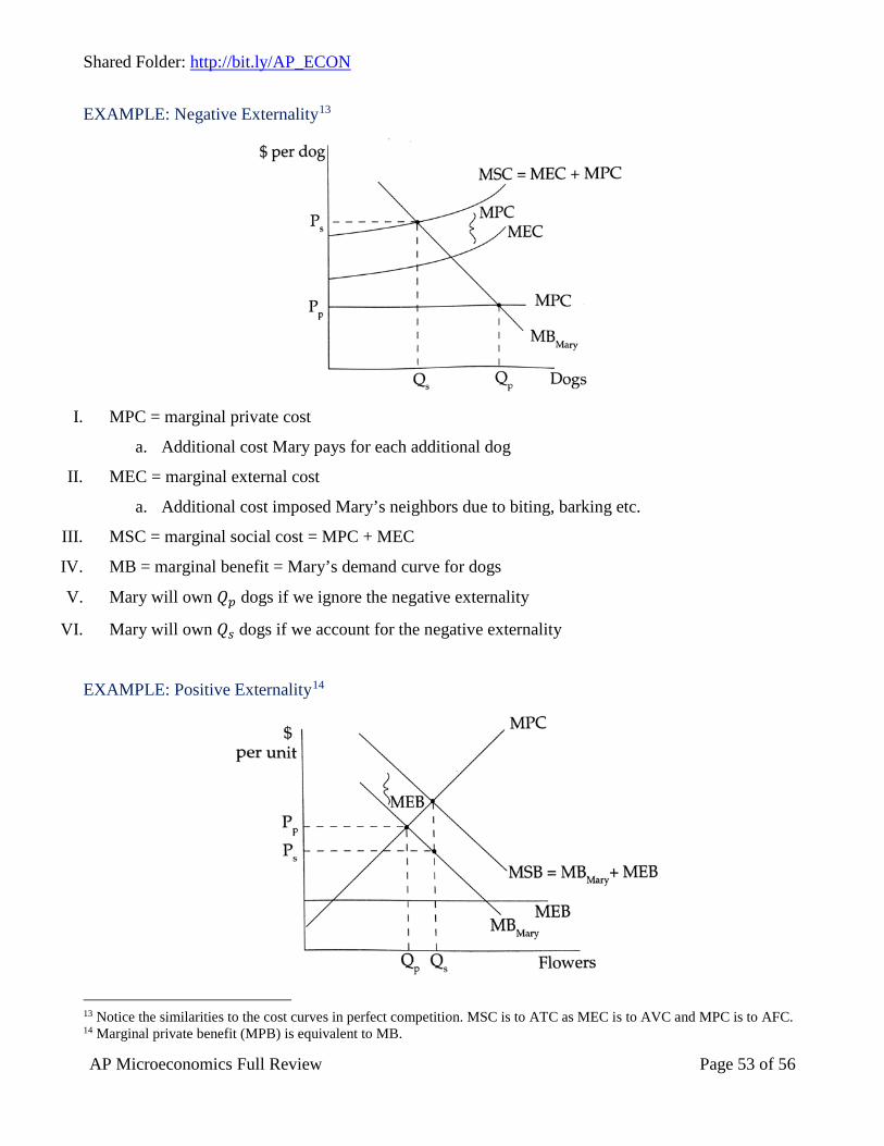
EXAMPLE: Negative Externality13

I. MPC = marginal private cost

a. Additional cost Mary pays for each additional dog

II. MEC = marginal external cost

a. Additional cost imposed Mary’s neighbors due to biting, barking etc.

III. MSC = marginal social cost = MPC + MEC

IV. MB = marginal benefit = Mary’s demand curve for dogs

V. Mary will own 𝑄𝑄𝑜𝑜 dogs if we ignore the negative externality

VI. Mary will own 𝑄𝑄𝑐𝑐 dogs if we account for the negative externality

EXAMPLE: Positive Externality14

13 Notice the similarities to the cost curves in perfect competition. MSC is to ATC as MEC is to AVC and MPC is to AFC. 14 Marginal private benefit (MPB) is equivalent to MB.


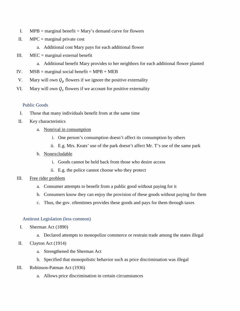
I. MPB = marginal benefit = Mary’s demand curve for flowers

II. MPC = marginal private cost

a. Additional cost Mary pays for each additional flower

III. MEC = marginal external benefit

a. Additional benefit Mary provides to her neighbors for each additional flower planted

IV. MSB = marginal social benefit = MPB + MEB

V. Mary will own 𝑄𝑄𝑜𝑜 flowers if we ignore the positive externality

VI. Mary will own 𝑄𝑄𝑐𝑐 flowers if we account for positive externality

Public Goods

I. Those that many individuals benefit from at the same time


a. Nonrival in consumption

i. One person’s consumption doesn’t affect its consumption by others

ii. E.g. Mrs. Keats’ use of the park doesn’t affect Mr. T’s use of the same park

b. Nonexcludable

i. Goods cannot be held back from those who desire access

ii. E.g. the police cannot choose who they protect

III. Free rider problem

a. Consumer attempts to benefit from a public good without paying for it

b. Consumers know they can enjoy the provision of these goods without paying for them

c. Thus, the gov. oftentimes provides these goods and pays for them through taxes

Antitrust Legislation (less common)

I. Sherman Act (1890)

a. Declared attempts to monopolize commerce or restrain trade among the states illegal

II. Clayton Act (1914)

a. Strengthened the Sherman Act

b. Specified that monopolistic behavior such as price discrimination was illegal

III. Robinson-Patman Act (1936)

a. Allows price discrimination in certain circumstances



i. E.g. differences in marketability of product

IV. Celler-Kefauver Act (1950)

a. Banned select vertical mergers

i. Merger of firms in the various steps in the production process

b. Banned select horizontal mergers

i. Merger of firms who are direct competitors

Measures of Market Power (less common)

I. Herfindahl-Harschman Index (HHI)

a. 𝐻𝐻𝐻𝐻𝐻𝐻 = ∑ 𝑆𝑆𝑜𝑜2𝑚𝑚𝑜𝑜=1

i. Takes the market share of each firm in an industry as a percentage, squares each

percentage, and adds them up

b. Increases as the number of firms in the industry decreases and/or as the firms become less

uniform in size

II. N-firm concentration ratio

a. Sum of the market shares of the largest n firms in an industry, where n is an integer

GRAPH: Lorenz Curve


I. Measure of income inequality

II. Horizontal axis starts with the poorest families on the left and ends with the richest families

III. Gini coefficient = 𝑐𝑐ℎ𝑡𝑡𝑝𝑝𝑐𝑐𝑝𝑝 𝑡𝑡𝑜𝑜𝑐𝑐𝑡𝑡𝑡𝑡𝑜𝑜𝑐𝑐𝑡𝑡 𝑜𝑜𝑓𝑓 ∆𝐴𝐴𝐴𝐴𝑇𝑇

a. If the Lorenz curve was the line of perfect equality, the poorest 𝑟𝑟% of people would own

𝑟𝑟% of the wealth in their nation: Gini coefficient = 0

b. United States Gini coefficient: 0.45

Poverty and Taxes

I. Poverty line

a. Official benchmark of poverty

II. Progressive tax

a. Gov. receives a larger percentage of revenue from families with larger incomes

III. Regressive tax15

a. Gov. receives a larger percentage of revenue from families with smaller incomes

IV. Proportional tax

a. Gov. receives the same percentage of income from all families

V. Social Security

a. Provides cash benefits and health insurance to retired and disabled works and their families

15 For example, Mrs. Keats employs a regressive curve in her class: the curve helps you more the worse you do.

Documents

AP Microeconomics Full Review - North Allegheny · AP ® Microeconomics Full Review . VERSION 2 ... Around 18% and 15% of people get 5s on the AP Micro and AP Macro ... Economics