Instrument modeling for High Contrast Imaging

Tips and tools

Anthony BoccalettiObservatoire de Paris

LESIA

Context

• Several instruments dedicated to Exoplanet detection and characterization with High Contrast Imaging since 2001

• For this decade : • SPHERE and GPI : 2011/12• JWST-MIRI : 2015

• For the future (>2020-25):• ELT / EPICS • Space coronagraphs : ACCESS, PECO, SPICES ….

=> need for simulation tools adapted to the instruments and to the observing cases

Favorite Techniques

Effects issues solutions

Stellar diffraction - photon flux- photon noise

coronagraphy

Wavefront errors (dynamic and static)

- speckle noise- photon noise

wavefront sensing and correction

Residual aberrations (mostly static)

- un-seen - un-corrected

speckle calibration differential imaging

Issues or noises related to Image formation (so to the source itself)

Many other sources of noise• Background : sky, thermal emission of instrument/telescope, zodiacal light,

exozodi• Detector related : Flat Field, readout noise, remanance, …• Many others that we don't even thought about !!!

Interest of instrument modeling

• Assess the performance for a science case• Evaluate the limitations : which source of noise, or which issues are

relevant ?• Put some constraints on the instrument design• Optimize the design itself (instrumental choices)

• And then => reassess the performance

Generic concept of a coronagraph

plan focal + diaphragmepupille

détecteur

pupille

FFTFFT-1

FFT

+ masque

Plan A Plan B Plan C Plan D

€

ψA

€

ψB

€

ψC

€

ψD

The mathematical formulation

€

ψA = A.e iϕ

€

ψA = A

€

ϕ =0siPlan A:

Plan B:

€

ψB =ψ A ⇒ ψ A .M

Plan C:

€

ψC =ψ B =ψ A ⊗M ⇒ ψ A ⊗M( ).D

Plan D:

€

ψD =ψC = ψ A .M( )⊗D

Problem … too many concepts

A good example : SPHERE

Common Path

Fore optics

Extreme AO

NI R Coronagraph

Vis Coronagraph

ZIMPOL

IFS

IRDIS

High frequency AO correction (41x41 act.)High stability : image / pupil controlVisible – NIR Refraction correctionFoV = 12.5’’40x40 SH-WFS in visible1.2 KHz, RON < 1e-

Pupil apodisation, Focal masks: Lyot, A4Q, ALC. IR-TT sensor for fine entering

Coronagraphic imaging:Dual polarimetry, direct BB + NB. λ = 0.5 – 0.9 µm, λ/2D @ 0.6 µm, FoV = 3.5”

0.95 – 1.35/1.65 µm λ/2D @ 0.95 µm, Spectral resolution: R = 54 / 33FoV = 1.77”

0.95 – 2.32 µm; λ/2D @ 0.95 µm Differential imaging: 2 wavelengths, R~30, FoV = 12.5’’Long Slit spectro: R~50 & 400Differential polarizationNasmyth platform, static bench,

Temperature control, cleanliness control Active vibration control

Beam control (DM, TT, PTT, derotation)Pola controlCalibration

Context and Issues

- characterization of Giant Planets and Brown Dwarves : contrast of 10-6 / 10-7 @ 0.5’’ - instrumentation : - exAO

- coronography

Calibration of the residual speckle pattern is needed

contrast ~ 6.10-5

Speckle calibration is needed

plan focal + diaphragmepupille

détecteur

différentiel

pupille

FFTFFT-1

FFT

+ masque

Plan A Plan B Plan C Plan D

€

ψA

€

ψB

€

ψC

€

ψD

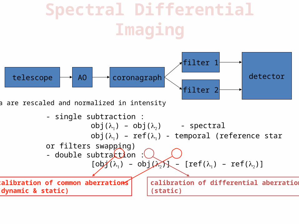
Spectral Differential Imaging

- single subtraction : obj() – obj() - spectralobj() – ref() - temporal (reference star or

filters swapping) - double subtraction :

[obj() – obj()] – [ref() – ref()]

telescope AO coronagraph

filter 2

filter 1

detector

data are rescaled and normalized in intensity

calibration of common aberrations(dynamic & static)

calibration of differential aberrations(static)

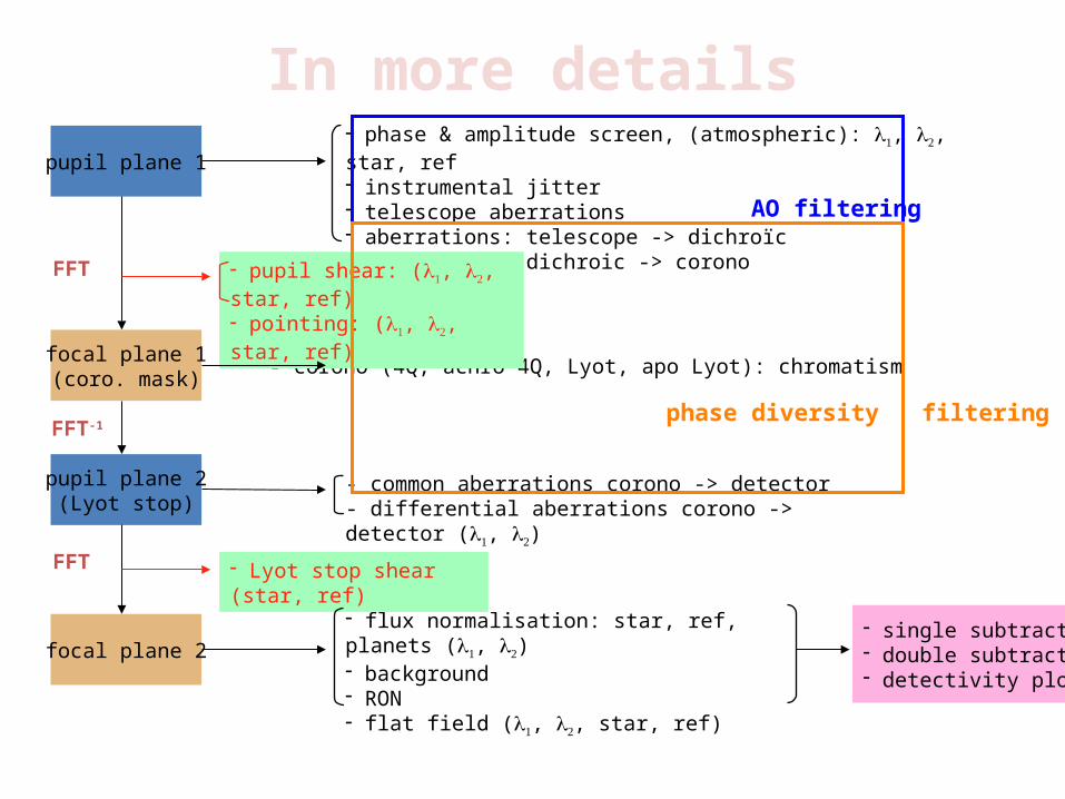
In more detailspupil plane 1

focal plane 2

focal plane 1(coro. mask)

pupil plane 2(Lyot stop)

- phase & amplitude screen, (atmospheric): , , star, ref- instrumental jitter- telescope aberrations- aberrations: telescope -> dichroïc- aberrations: dichroic -> corono

- common aberrations corono -> detector- differential aberrations corono -> detector (, )

- flux normalisation: star, ref, planets (, )- background- RON- flat field (, , star, ref)

- corono (4Q, achro 4Q, Lyot, apo Lyot): chromatism

- pupil shear: (, , star, ref)- pointing: (, , star, ref)

- Lyot stop shear (star, ref)

FFT

FFT-1

FFT

- single subtraction- double subtraction- detectivity plot

AO filtering

phase diversity filtering

SPHERE simulation with CAOS

SPHERE simulation with CAOS

SPHERE simulation with CAOS

SPHERE simulation with CAOS

Some tips to begin with …

• Sampling of the pupil : • good sampling needed to reproduce pupil shape• Make use of grey approx.

• Sampling of the image• PSF size = N / D = lambda/D

(N: array size, D: pupil diameter)

• PSF chromaticity• Modify pupil size but keep the array constant => change the actual

shape of the pupil• Modify array size but keep the pupil constant

• Uses of FFT with IDL• Shift the center to coordinates [0,0]• Aliasing: make sure N is at least 2xD

Some tips to begin with …

• Image normalization: • use an off-axis object far from the center (not affected by the mask) but

account for the throughput

• Wavefront errors:• Define the Power Spectrum Density of aberrations with power law and

cut-off frequencies• WFE screen = random screen X sqrt (PSD)

The exercise

• Produce coronagraphic images at two simultaneous wavelengths for a star and a reference target. Compare contrast curves (5s) at different stages: coronagraphic image, 2-l subtraction, ref-subtraction, double subtraction

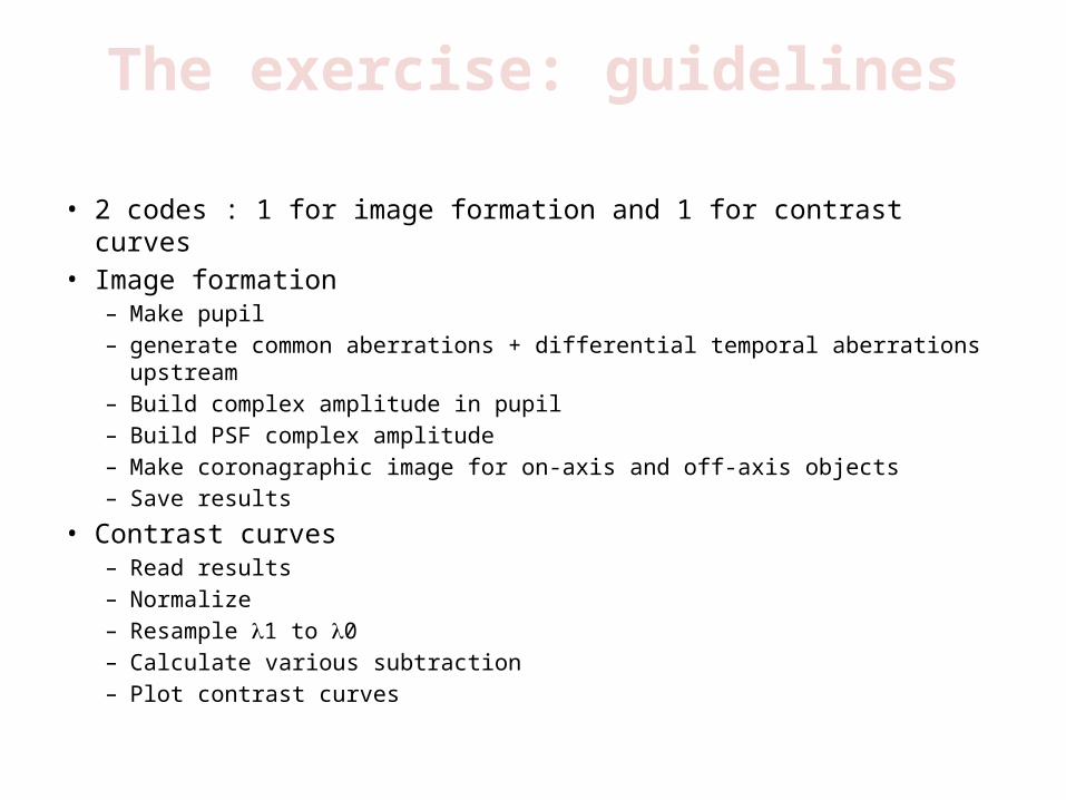
The exercise: guidelines

• 2 codes : 1 for image formation and 1 for contrast curves• Image formation

– Make pupil– generate common aberrations + differential temporal aberrations upstream– Build complex amplitude in pupil– Build PSF complex amplitude– Make coronagraphic image for on-axis and off-axis objects– Save results

• Contrast curves– Read results– Normalize– Resample l1 to l0– Calculate various subtraction– Plot contrast curves

The exercise: guidelines

• Image formation– Start with circular pupil then use the routine sph_pupil to produce VLT pupil in

grey level. – Generate diaphragm (under/over-sized)– Define bands: H2 H3 filters of SPHERE = 1.593 & 1.667 microns – upstream aberrations :

• use the provided VLT_wfe.fits• Add a 4nm defocus on the reference target

– Define a loop on filter and scale array size accordingly– Calculate complex amplitude in pupil : sph_amp_complex.pro– Build PSFs with sph_psf.pro– Introduce differential aberrations with sph_wfdiff.pro– Build coronagraphic images with sph_corono.pro– Take intensities– Rescale the arrays to 1kx1k with sph_taille.pro– Produce off-axis planets with sph_planet.pro– Save results

The exercise: guidelines

• Contrast curves:– Read results of image formation– Resample to camera pixels (shannon at 0.95mic) make use of

sph_rescale.pro– Resample of image at l1 to l0 (again sph_rescale.pro)– Calculate subtractions:

• obj(l0)-ref(l0)• obj(l0)-obj(l1)• [obj(l0)-obj(l1)] – [ref(l0)-ref(l1)]

– Azimuthal contours with sph_profil1d.pro– Plot averaged contour for psf and corono image and 5sig level for subtractions

The exercise: guidelines

• And play with the parameters ….

• D = 8m / 160 pix• N = 1024• 40 linear actuators• Relative offset (star/ref) = 0.5 mas• Differential aberrations = 10nm• Planet separations = 0.1", 0.5", 1"

More tools …

• Reference to :– CAOS + SPHERE Software package (public)– PROPER by John Krist (public)– PESCA for ELT (not public)