Embed Size (px)
Citation preview

ANTENNAS FORGLOBAL NAVIGATIONSATELLITE SYSTEMS

ANTENNAS FORGLOBAL NAVIGATIONSATELLITE SYSTEMS
Xiaodong ChenQueen Mary University of London, UK
Clive G. PariniQueen Mary University of London, UK
Brian CollinsAntenova Ltd, UK
Yuan YaoBeijing University of Posts and Telecommunications, China
Masood Ur RehmanQueen Mary University of London, UK
A John Wiley & Sons, Ltd., Publication
This edition first published 2012© 2012 John Wiley & Sons Ltd
Registered officeJohn Wiley & Sons Ltd, The Atrium, Southern Gate, Chichester, West Sussex, PO19 8SQ, UnitedKingdom
For details of our global editorial offices, for customer services and for information about how to applyfor permission to reuse the copyright material in this book please see our website at www.wiley.com.
The right of the authors to be identified as the authors of this work has been asserted in accordancewith the Copyright, Designs and Patents Act 1988.
All rights reserved. No part of this publication may be reproduced, stored in a retrieval system, ortransmitted, in any form or by any means, electronic, mechanical, photocopying, recording orotherwise, except as permitted by the UK Copyright, Designs and Patents Act 1988, without the priorpermission of the publisher.
Wiley also publishes its books in a variety of electronic formats. Some content that appears in printmay not be available in electronic books.
Designations used by companies to distinguish their products are often claimed as trademarks. Allbrand names and product names used in this book are trade names, service marks, trademarks orregistered trademarks of their respective owners. The publisher is not associated with any product orvendor mentioned in this book. This publication is designed to provide accurate and authoritativeinformation in regard to the subject matter covered. It is sold on the understanding that the publisheris not engaged in rendering professional services. If professional advice or other expert assistance isrequired, the services of a competent professional should be sought.
Library of Congress Cataloging-in-Publication Data
Antennas for global navigation satellite systems / Xiaodong Chen . . . [et al.].p. cm.
Includes bibliographical references and index.ISBN 978-1-119-99367-4 (cloth)
1. Antennas (Electronics) 2. Global Positioning System. 3. Space vehicles–Radio antennas.4. Radio wave propagation. 5. Mobile communication systems. I. Chen, Xiaodong.
TK7871.6.A532 2012621.382–dc23
2011043939
A catalogue record for this book is available from the British Library.
ISBN: 9781119993674
Set in 10.5/13pt Times by Laserwords Private Limited, Chennai, India

Contents
Preface ix
1 Fundamentals of GNSS 11.1 History of GNSS 11.2 Basic Principles of GNSS 2
1.2.1 Time-Based Radio Navigation 21.2.2 A 3D Time-Based Navigation System 5
1.3 Operation of GPS 81.4 Applications Including Differential GPS 15
References 18
2 Fundamental Considerations for GNSS Antennas 212.1 GNSS Radio Wave Propagation 21
2.1.1 Plane Waves and Polarisation 212.1.2 GNSS Radio Wave Propagation and Effects 232.1.3 Why CP Waves in GNSS? 26
2.2 Antenna Design Fundamentals 262.2.1 Antenna Fundamental Parameters 262.2.2 LP Antenna Design and Example 29
2.3 CP Antenna Design 312.3.1 CP Antenna Fundamentals and Types 312.3.2 Simple CP Antenna Design Example 352.3.3 Technical Challenges in Designing GNSS Antennas 36References 40
3 Satellite GNSS Antennas 413.1 Navigation Antenna Requirements 413.2 Types of Antenna Deployed 41
vi Contents
3.3 Special Considerations for Spacecraft Antenna Design 503.3.1 Passive Intermodulation Effects 503.3.2 Multipactor Effects 52References 52
4 Terminal GNSS Antennas 554.1 Microstrip Antenna for Terminal GNSS Application 55
4.1.1 Single-Feed Microstrip GNSS Antennas 554.1.2 Dual-Feed Microstrip GNSS Antennas 604.1.3 Design with Ceramic Substrate 64
4.2 Spiral and Helix GNSS Antennas 664.2.1 Helix Antennas 664.2.2 Spiral Antennas 71
4.3 Design of a PIFA for a GNSS Terminal Antenna 73References 79
5 Multimode and Advanced Terminal Antennas 815.1 Multiband Terminal Antennas 81
5.1.1 Multiband Microstrip GNSS Antennas 825.1.2 Multiband Helix Antennas for GNSS 88
5.2 Wideband CP Terminal Antennas 955.2.1 Wideband Microstrip Antenna Array 955.2.2 High-Performance Universal GNSS Antenna Based
on Spiral Mode Microstrip Antenna Technology 965.2.3 Wideband CP Hybrid Dielectric Resonator Antenna 965.2.4 Multi-Feed Microstrip Patch Antenna for Multimode
GNSS 985.3 High-Precision GNSS Terminal Antennas 102
References 109
6 Terminal Antennas in Difficult Environments 1116.1 GNSS Antennas and Multipath Environment 1116.2 Statistical Modelling of Multipath Environment for GNSS
Operation 1136.2.1 GPS Mean Effective Gain (MEGGPS) 1146.2.2 GPS Angle of Arrival Distribution (AoAGPS) 1166.2.3 GPS Coverage Efficiency (ηc) 117
6.3 Open Field Test Procedure 1196.3.1 Measurement of GPS Mean Effective Gain 119

Contents vii
6.3.2 Measurement of GPS Coverage Efficiency 1206.3.3 Measurement Set-Up 120
6.4 Performance Assessment of GNSS Mobile Terminal Antennasin Multipath Environment 1216.4.1 Design of Tested GPS Antennas 1226.4.2 Comparison Based on Simulated and Measured 3D
Radiation Patterns 1276.4.3 Comparison Based on Measured 3D Radiation
Patterns and Actual Field Tests 1296.5 Performance Dependence on GNSS Antenna Orientation 1336.6 Performance Enhancement of GNSS Mobile Terminal
Antennas in Difficult Environments 1396.6.1 Assisted GPS 1406.6.2 GPS Signal Reradiation 1406.6.3 Beamforming 1416.6.4 Diversity Antennas 141References 147
7 Human User Effects on GNSS Antennas 1497.1 Interaction of Human Body and GNSS Antennas 1497.2 Effects of Human Body on GNSS Mobile Terminal Antennas
in Difficult Environments 1507.2.1 Design of Tested GPS Antennas 1517.2.2 Effects of Human Hand and Head Presence 1517.2.3 Effects of Complete Human Body Presence 166References 179
8 Mobile Terminal GNSS Antennas 1818.1 Introduction 1818.2 Antenna Specification Parameters 183
8.2.1 Polarisation 1838.2.2 Radiation Patterns 1848.2.3 Impedance 1858.2.4 Gain/Efficiency 1868.2.5 Weight 1878.2.6 Bandwidth 1878.2.7 Phase Performance 188
8.3 Classification of GNSS Terminals 1888.3.1 Geodetic Terminals 188
viii Contents
8.3.2 Rover Terminals 1888.3.3 General Purpose Mobile Terminals 189
8.4 Antenna Designs for Portable User Equipment 1908.4.1 Short Quadrifilar Helices 1908.4.2 Patch Antennas 1918.4.3 Smaller Antennas 192
8.5 The Function of the Platform 1928.5.1 Antenna Efficiency, Gain and Noise 193
8.6 Comparing Antenna Performance on UEs 1948.6.1 Drive Testing 1948.6.2 Non-Antenna Aspects of Performance 195
8.7 Practical Design 1978.7.1 Positioning the GNSS Antenna on the Application
Platform 1978.7.2 Evaluating the Implementation 200
8.8 Case Studies 2018.8.1 Measurement System 2018.8.2 Case 1: Modified PIFA on Face of Small PCB 2028.8.3 Case 2: Meandered Dipole Antenna on Top Edge of
Small PCB 2038.8.4 Case 3: Modified PIFA above LCD Display on
Smart-Phone-Size Device 2048.8.5 Case 4: Moving Modified PIFA from One to Adjacent
Corner of PCB 2058.8.6 Cases 5 and 6: Effects of Platform Electronics Noise 205
8.9 Summary 206References 206
Appendix A Basic Principle of Decoding Information from aCDMA Signal 207
Appendix B Antenna Phase Characteristics and Evaluation ofPhase Centre Stability 211
Index 215

Preface
The global navigation satellite system (GNSS) is becoming yet another pillartechnology in today’s society along with the Internet and mobile commu-nications. GNSS offers a range of services, such as navigation, positioning,public safety and surveillance, geographic surveys, time standards, mapping,and weather and atmospheric information. The usage of GNSS applications hasbecome nearly ubiquitous from the ever-growing demand of navigation facil-ities made available in portable personal navigation devices (PNDs). Sales ofmobile devices including smart phones with integrated GNSS are expected togrow from 109 million units in 2006 to 444 million units in 2012, and this sectorof industry is second only to the mobile phone industry. The navigation industryis predicted to earn a gross total of $130 billion in 2014. The current develop-ments and expected future growth of GNSS usage demand the availability ofmore sophisticated terminal antennas than those previously deployed.
The antenna is one of most important elements on a GNSS device. GNSSantennas are becoming more complex every day due to the integration of dif-ferent GNSS services on one platform, miniaturisation of these devices andperformance degradations caused by the user and the local environment. Thesefactors should be thoroughly considered and proper solutions sought in orderto develop efficient navigation devices. The authors have been active in thisresearch area over the last decade and are aware that a large amount of infor-mation on GNSS antenna research is scattered in the literature. There is thus aneed for a coherent text to address this topic, and this book intends to fill thisknowledge gap in GNSS antenna technology. The book focuses on both thetheory and practical designs of GNSS antennas. Various aspects of GNSS anten-nas, including the fundamentals of GNSS and circularly polarised antennas,design approaches for the GNSS terminal and satellite antennas, performanceenhancement techniques used for such antennas, and the effects of a user’spresence and the surrounding environment on these antennas, are discussed

x Preface
in the book. Many challenging issues of GNSS antenna design are addressedgiving solutions from technology and application points of view.
The book is divided into eight chapters.Chapter 1 introduces the concept of GNSS by charting its history starting
from DECCA land-based navigation in the Second World War to the latest ver-sions being implemented by the USA (GPS), Europe (GLONASS and Galileo)and China (Compass). The fundamental principles of time delay navigationare addressed and the operation of the US NAVSTAR GPS is described. Theenhanced applications of the GPS are addressed including its use as a timereference and as an accurate survey tool in its differential form.
Chapter 2 describes radio wave propagation between the GNSS satellite andthe ground receiver and the rationale for selecting circularly polarised (CP)waves. It also introduces the relevant propagation issues, such as multipathinterference, RF interference, atmospheric effects, etc. The fundamental issuesin GNSS antenna design are highlighted by presenting the basic approaches fordesigning a CP antenna.
Chapter 3 covers the requirements for spacecraft GNSS antennas illustrat-ing the descriptions of typical deployed systems for both NAVSTAR GPS andGalileo. The various special performance requirements and tests imposed onspacecraft antennas, such as passive intermodulation (PIM) testing and multi-pactor effects, are also discussed.
Chapter 4 deals with the specifications, technical challenges, design method-ology and practical designs of portable terminal GNSS antennas. It introducesvarious intrinsic types of terminal antennas deployed in current GNSSs, includ-ing microstrip, spiral, helical and ceramic antennas.
Chapter 5 is dedicated to multimode antennas for an integrated GNSSreceiver. The chapter presents three kinds of multimode GNSS antennas,namely dual-band, triple-band and wideband antennas. Practical and novelantenna designs, such as multi-layer microstrip antennas and couple feed slotantennas, are discussed. It also covers high-precision terminal antennas for thedifferential GPS system, including phase centre determination and stability.
Chapter 6 discusses the effects of the multipath environment on the perfor-mance of GNSS antennas in mobile terminals. It highlights the importance ofstatistical models defining the environmental factors in the evaluation of GNSSantenna performance and proposes such a model. It then presents a detailedanalysis of the performance of various types of mobile terminal GNSS anten-nas in real working scenarios using the proposed model. Finally, it describesthe performance enhancement of the terminal antennas in difficult environmentsby employing the techniques of beamforming, antenna diversity, A-GPS andESTI standardised reradiating.

Preface xi
Chapter 7 deals with the effects of the human user’s presence on the GNSSantennas, presenting details of the dependency of antenna performance onvarying antenna–body separations, different on-body antenna placements andvarying body postures. It also considers the effects of homogeneous and inho-mogeneous human body models in the vicinity of the GNSS antennas. Finally,it discusses the performance of these antennas in the whole multipath environ-ment operating near the human body, using a statistical modelling approachand considering various on-body scenarios.
Chapter 8 describes the limitations of both antenna size and shape that areimposed when GNSS functions are to be added to small devices such as mobilehandsets and personal trackers. It is shown how the radiation patterns andpolarisation properties of the antenna can be radically changed by factors suchas the positioning of the antenna on the platform. The presence of a highlysensitive receiver system imposes severe constraints on the permitted levels ofnoise that may be generated by other devices on the platform without impairingthe sensitivity of the GPS receiver. The chapter gives the steps which must betaken to reduce these to an acceptable level. The case studies cover a rangeof mobile terminal antennas, such as small backfire helices, CP patches andvarious microstrip antennas.
This is the first dedicated book to give such a broad and in-depth treatmentof GNSS antennas. The organisation of the book makes it a valuable practicalguide for antenna designers who need to apply their skills to GNSS applications,as well as an introductory text for researchers and students who are less familiarwith the topic.

1Fundamentals of GNSS
1.1 History of GNSS
GNSS is a natural development of localised ground-based systems such asthe DECCA Navigator and LORAN, early versions of which were used inthe Second World War. The first satellite systems were developed by the USmilitary in trial projects such as Transit, Timation and then NAVSTAR, theseoffering the basic technology that is used today. The first NAVSTAR waslaunched in 1989; the 24th satellite was launched in 1994 with full operationalcapability being declared in April 1995. NAVSTAR offered both a civilian and(improved accuracy) military service and this continues to this day. The systemhas been continually developed, with more satellites offering more frequenciesand improved accuracy (see Section 1.3).
The Soviet Union began a similar development in 1976, with GLONASS(GLObal NAvigation Satellite System) achieving a fully operational constella-tion of 24 satellites by 1995 [1]. GLONASS orbits the Earth, in three orbitalplanes, at an altitude of 19 100 km, compared with 20 183 km for NAVSTAR.Following completion, GLONASS fell into disrepair with the collapse of theSoviet economy, but was revived in 2003, with Russia committed to restoringthe system. In 2010 it achieved full coverage of the Russian territory with a20-satellite constellation, aiming for global coverage in 2012.
The European Union and European Space Agency Galileo system consistsof 26 satellites positioned in three circular medium Earth orbit (MEO) planes at23 222 km altitude. This is a global system using dual frequencies, which aimsto offer resolution down to 1 m and be fully operational by 2014. Currently(end 2010) budgetary issues mean that by 2014 only 18 satellites will be oper-ational (60% capacity).
Antennas for Global Navigation Satellite Systems, First Edition.Xiaodong Chen, Clive G. Parini, Brian Collins, Yuan Yao and Masood Ur Rehman.© 2012 John Wiley & Sons, Ltd. Published 2012 by John Wiley & Sons, Ltd.

2 Antennas for Global Navigation Satellite Systems
Compass is a project by China to develop an independent regional and globalnavigation system, by means of a constellation of 5 geostationary orbit (GEO)satellites and 30 MEO satellites at an altitude of 21 150 km. It is planned tooffer services to customers in the Asia-Pacific region by 2012 and a globalsystem by 2020.
QZSS (Quasi-Zenith Satellite System) is a Japanese regional proposal aimedat providing at least one satellite that can be observed at near zenith over Japanat any given time. The system uses three satellites in elliptical and inclinedgeostationary orbits (altitude 42 164 km), 120◦ apart and passing over the sameground track. It aims to work in combination with GPS and Galileo to improveservices in city centres (so called urban canyons) as well as mountainousareas. Another aim is for a 1.6 m position accuracy for 95% availability, withfull operational status expected by 2013.
It is likely that many of these systems will offer the user interoperabilityleading to improved position accuracy in the future. It has already been shownthat a potential improvement in performance by combining the GPS and Galileonavigation systems comes from a better satellite constellation compared witheach system alone [2]. This combined satellite constellation results in a lowerdilution of precision value (see Section 1.3), which leads to a better positionestimate. A summary of the various systems undertaken during the first quarterof 2011 is shown in Table 1.1.
1.2 Basic Principles of GNSS
1.2.1 Time-Based Radio Navigation
The principle of GNSSs is the accurate measurement of distance from thereceiver of each of a number (minimum of four) of satellites that transmitaccurately timed signals as well as other coded data giving the satellites’ posi-tion. The distance between the user and the satellite is calculated by knowingthe time of transmission of the signal from the satellite and the time of recep-tion at the receiver, and the fact that the signal propagates at the speed of light.From this a 3D ranging system based on knowledge of the precise positionof the satellites in space can be developed. To understand the principles, thesimple offshore maritime 2D system shown in Figure 1.1 can be considered.Imagine that transmitter 1 is able to transmit continually a message that says‘on the next pulse the time from transmitter 1 is . . . ’, this time being sourcedfrom a highly accurate (atomic) clock. At the mobile receiver (a ship in thisexample) this signal is received with a time delay �T 1; the distance D1 fromthe transmitter can then be determined based on the signal propagating at the

Fundamentals of GNSS 3
Tabl
e1.
1Su
mm
ary
ofG
NSS
syst
ems
unde
rtak
endu
ring
Q1
2011
GN
SSG
PS/N
AV
STA
RG
LO
NA
SSG
alile
oC
ompa
ssQ
ZSS
Ope
ratio
nal
Now
Now
2014
(for
14sa
telli
tes)
2012
regi
onal
2020
glob
al20
13
Con
stel
latio
n24
ME
O24
ME
O27
ME
O5
GE
O+
30M
EO
3hi
ghly
incl
ined
ellip
tical
orbi
tsO
rbita
lal
titud
e(k
m)
2018
319
100
2322
221
150
+G
EO
4216
4C
over
age
Glo
bal
Reg
iona
l(R
ussi
a)th
engl
obal
Glo
bal
Reg
iona
l(A
sia-
Paci
fic)
then
glob
al
Reg
iona
l(E
ast
Asi
aan
dO
cean
ia),
augm
enta
tion
with
GPS
Posi
tion
accu
racy
(civ
ilian
)7.
1m
95%
7.5
m95
%4
m(d
ual
freq
.)10
m1.
6m
95%
Use
rFr
eque
ncy
band
s(M
Hz)
L1
=15
75.4
20L
2=
1227
.6L
5=
1176
.45
G1
=16
02.0
G2
=12
46.0
G3
=12
04.7
04
E1
=15
75.4
2E
6=
1278
.75
E5
=11
91.7
95E
5a=
1176
.45
E5b
=12
07.1
4
B1
=15
61.0
98B
2=
1207
.14
B3
=12
68.5
2
L1
L2
L5
LE
X=
1278
.75
(for
Dif
fere
ntia
lG
PS)
Use
rco
ding
and
mod
ulat
ion
CD
MA
BPS
KFD
MA
BPS
K+
CD
MA
onG
LO
NA
SS-K
1
CD
MA
BO
Can
dB
PSK
QPS
Kan
dB
OC
CD
MA
BPS
K,
BO
C
Serv
ices
and
band
wid
thSP
Son
L1
with
2.04
6M
Hz
BW
PPS
onL
1&
L2
with
20.4
6M
Hz
BW
L2C
(by
2016
)L
5(b
y20
18)
20.4
6M
Hz
BW
Ope
non
E1
with
24.5
52M
Hz
BW
Ope
non
E5a
+E
5bbo
th20
.46
MH
zB
W
Ope
non
B1
with
4.09
2M
Hz
BW
Ope
non
B2
with
24M
Hz
BW
L1
24M
Hz
BW
,L
224
MH
zB
W,
L5
24.9
MH
zB
W
CD
MA
:C
ode
Div
isio
nM
ultip
leA
cces
s;FD
MA
:Fr
eque
ncy
Div
isio
nM
ultip
leA
cces
s;B
PSK
:B
inar
yPh
ase
Shif
tK
eyin
g;Q
PSK
:Q
uadr
atur
ePh
ase
Shif
tK
eyin
g;B
OC
:B
inar
yO
ffse
tC
arri
er;
SPS:
Stan
dard
Posi
tioni
ngSe
rvic
e;PP
S:Pr
ecis
ion
Posi
tioni
ngSe
rvic
e.

4 Antennas for Global Navigation Satellite Systems
Frequency F2My time is T2
Synchronised clock
Frequency F1My time is T1
D2 = cΔT2
D1 = cΔT1
Figure 1.1 Simple 2D localised ship-to-shore location system.
speed of light c, from D1 = c�T 1. The same process can be repeated fortransmitter 2, yielding a distance D2. If the mobile user then has a chart showingthe accurate location of the shore-based transmitter 1 and transmitter 2, theuser can construct the arcs of constant distance D1 and D2 and hence findhis or her location. For this system to be accurate all three clocks (at the twotransmitters and on board the ship) must be synchronised. In practice it maynot be that difficult to synchronise the two land-based transmitters but thelevel of synchronisation of the ship-based clock will fundamentally determinethe level of position accuracy achievable. If the ship’s clock is in error by±1 μs then the position error will be ±300 m, since light travels 300 m ina microsecond. This is the fundamental problem with this simplistic systemwhich can be effectively thought of as a problem of two equations with twounknowns (the unknowns being the ship’s ux , uy location). However, in realitywe have a third unknown, which is the ship’s clock offset with respect to thesynchronised land-based transmitters’ clock. This can be overcome by addinga third transmitter to the system, providing the ability to add a third equationdetermining the ux , uy location of the ship and so giving a three-equation,
Fundamentals of GNSS 5
three-unknown solvable system of equations. We will explore this in detaillater when we consider the full 3D location problem that is GNSS. As a localcoastal navigation system this is practical since all ships will be south of thetransmitters shown in Figure 1.1.
At this point it is worth noting the advantages of this system, the key onebeing that the ship requires no active participation in the system; it is onlyrequired to listen to the transmissions to determine its position. Thus, there isno limit on the number of system users and, because they are receive only,they will be relatively low cost for the ship owner.
1.2.2 A 3D Time-Based Navigation System
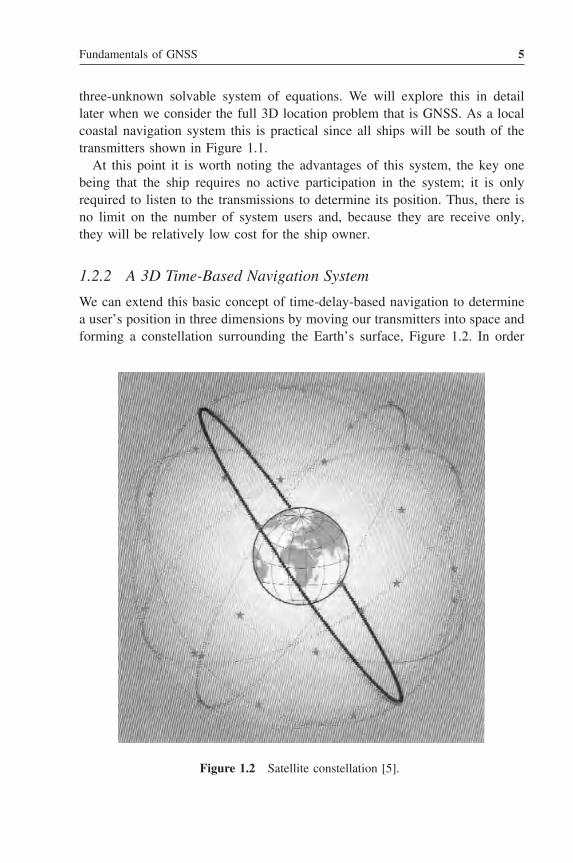
We can extend this basic concept of time-delay-based navigation to determinea user’s position in three dimensions by moving our transmitters into space andforming a constellation surrounding the Earth’s surface, Figure 1.2. In order
Figure 1.2 Satellite constellation [5].

6 Antennas for Global Navigation Satellite Systems
for such a system to operate the user would be required to see (i.e. have adirect line of sight to) at least four satellites at any one time. This time fourtransmitters are required as there are now four unknowns in the four equationsthat determine the distance from a satellite to a user, these being the user’scoordinates (ux , uy , uz ) and the user’s clock offset �T with respect to GPStime. The concept of GPS time is that all the clocks on board all the satellites arereading exactly the same time. In practice they use one (or more) atomic clocks,but by employing a series of ground-based monitoring stations each satelliteclock can be checked and so any offset from GPS time can be transmitted tothe satellite and passed on to the user requiring a position fix.
The (x , y , z ) location of each satellite used in a position fix calculation mustbe accurately known, and although Kepler’s laws of motion do a very goodjob in predicting the satellite’s location, use of the above-mentioned monitor-ing stations can offer minor position corrections. These monitoring stations(whose accurate position is known) can be used to determine accurately thesatellite’s orbital location and thus send to each satellite its orbital positioncorrections, which are then reported to the users via the GPS transmitted sig-nal to all users. So each satellite would effectively transmit ‘on the next pulsethe time is . . . , my clock offset from GPS time is . . . , my orbital positioncorrection is . . . ’.
A sketch of a four-satellite position location is shown in Figure 1.3 and thecorresponding equation for the raw distance R1 between the user terminal andsatellite 1 is
R1 = c(�t1 + �T − τ1) (1.1)
where �t1 is the true propagation delay from satellite 1 to the user terminal, τ 1is the GPS time correction for satellite 1, and �T is the unknown user terminalclock offset from GPS time. Let the corrected range to remove the satellite 1clock error be R′
1. Then
R′1 = c(�t1 + �T ) (1.2)
The true distance between satellite 1 and the user terminal is then
C�t1 = R′1 − c�t = R′
1 − CB (1.3)
where C B is fixed for a given user terminal at a given measurement time.In Cartesian coordinates the equation for the distance between the truesatellite 1 position (x1, y1, z 1), which has been corrected at the user terminal

Fundamentals of GNSS 7
User = Ux Uy Uz
R3
R2
R1
R4
L1 and L2 downlinks
My time is...My position is....
Figure 1.3 Sketch of four-satellite fix.
by the transmitted orbital correction data, and the user terminal position (ux ,uy , uz ) is
(x1 − ux)2 + (y1 − uy)
2 + (z1 − uz)2 = (R′
1 − CB)2 (1.4)
The corresponding equations for the remaining three satellites are
(x2 − ux)2 + (y2 − uy)
2 + (z2 − uz)2 = (R′
2 − CB)2
(x3 − ux)2 + (y3 − uy)
2 + (z3 − uz)2 = (R′
3 − CB)2
(x4 − ux)2 + (y4 − uy)
2 + (z4 − uz)2 = (R′
4 − CB)2
(1.5)
Equations 1.4 and 1.5 constitute four equations in four unknowns (ux , uy ,uz , C B ) and so enable the user terminal location to be determined.
In a similar way the user terminal’s velocity can be determined by measuringthe Doppler shift of the received carrier frequency of the signal from each ofthe four satellites. As in the case of time, an error due to the offset of the

8 Antennas for Global Navigation Satellite Systems
receiver oscillator frequency with GPS time can be removed using a four-satellite measurement. A set of equations with the three velocity componentsplus this offset again gives four equations with four unknowns (V x , V y , V z
and the user oscillator offset).
1.3 Operation of GPS
In this section we will take the basic concept described above and describehow a practical system (NAVSTAR GPS) can be implemented. As explainedabove, the user must be able to see four satellites simultaneously to get afix, so the concept of a constellation of MEO satellites (altitude 20 183 km)with 12 h circular orbits inclined at 55◦ to the equator in six orbital planes wasconceived [3]. With four satellites per orbital plane the operational constellationis 24 satellites (Figure 1.2); in 2010 the constellation had risen to 32 satellites.Figure 1.4 shows the satellite trajectories as viewed from the Earth for twoorbits (24 hours) with one satellite’s orbit shown by the heavy line for clarity.
This pattern repeats every day, although a given satellite in a given place isseen four minutes earlier each day. Assuming an open (non-urban) environment,the four ‘seen’ satellites need to be above a 15◦ elevation angle in order toavoid problems with multipath propagation. As we can see from Figure 1.5,this can be achieved at all points on the Earth’s surface, even at the poles.
60°
0° 30° 60° 90° 120° 150° 180° –150° –120° –90° –60° –30° 0°
0° 30° 60° 90° 120° 150° 180° –150° –120° –90° –60° –30° 0°
0°
–30°
30°
–60°
60°
0°
–30°
30°
–60°
Figure 1.4 Satellite trajectories as viewed from Earth for two orbits (24 hours) withone satellite’s orbit emphasised for clarity [5].

Fundamentals of GNSS 9
0°
180°
30°60
°
240°
210°
120°
300°
150°
330°
90°
270°
0°
180°
30°
60°
240°
210°
120°
300°
150°
330°
90°
270°
0°
180°
30°
60°
240°
210°
120°
300°
150°
330°
90°
270°
At Poles At 45 degree latitude(London 52 degrees)
Equator
Stars represent satellite position at any one time, heavy line is track for one satelliteCentre of sky chart is zenith, outer circle is the horizon
Figure 1.5 View of constellation from a user [5].
Ranger error
Figure 1.6 A 2D representation of range error as a function of satellite relativeposition (Shaded area represents region of position uncertainty).
Careful choice of location of the four satellites used for a fix can helpaccuracy, as can be simply illustrated in the 2D navigation system shown inFigure 1.6 and termed dilution of precision . The concept is of course extendableto the full 3D constellation of GPS.
GPS time is maintained on board the satellites by using a caesium and pairof rubidium atomic clocks providing an accuracy of better than 1 ns, whichis improved by passing onto the user the clock adjustments determined by

10 Antennas for Global Navigation Satellite Systems
L1 and L2 downlinks
L1 and L2 downlinks
Mastercontrol
Monitoringstation
S-bandUplink = 1783 MHzDownlink = 2227 MHz
Figure 1.7 Ground control segment monitoring one satellite in the constellation.
the ground control segment of the GPS system. An overview of the groundcontrol segment is shown in Figure 1.7 and consists of a master control station(MCS) and a number of remote monitoring stations distributed around theglobe. These monitoring stations passively track the GPS satellites as theypass overhead, making accurate range measurements and forwarding this datato the MCS via other satellite and terrestrial communication links. The MCSthen processes the data for each satellite in the constellation in order to provide:(i) clock corrections; (ii) corrections to the satellite’s predicted position in space(ephemeris)1 (i.e. its deviation from Kepler’s modified laws), typically validfor four hours; (iii) almanac data that tells the receiver which satellites shouldbe visible at a given time in the future and valid for up to 180 days. Thisdata is combined with the normal TT&C (Telemetry Tracking and Command)data and uplinked to each satellite via the TT&C communications link, whichfor the GPS satellites operates in the S band (2227 MHz downlink, 1783 MHzuplink). The uplink ground stations are located at a number of the remotemonitoring stations.
1 A table of values that gives the positions of astronomical objects in the sky at a given time.

Fundamentals of GNSS 11
The user communications downlink (Figure 1.7) is transmitted using RHCP(Right Hand Circular Polarisation) and has two operating modes:
1. Standard Positioning Service (SPS) – unrestricted access using the bandL1 = 1575.42 MHz.
2. Precision Positioning Service (PPS) – DoD (US Department of Defense)authorised users only using both bands L1 = 1575.42 MHz and L2 =1227.6 MHz.
Both L1 and L2 use CDMA (Code Division Multiple Access) as the multiplex-ing process and BPSK (Binary Phase Shift Keying) as the modulation method.As in all CDMA systems, all the satellites transmit at the same frequency buteach uses a different and unique ‘gold code’ as the spreading code for thisspread-spectrum form of communication. The basic CDMA process is that ofmultiplying each bit of information to be sent by a unique pseudo-random ‘goldcode’ (called the spreading code). If the information bit is logic 1 the gold codeis sent; if logic 0, the inverse of the gold code is sent. The encoded informationis then sent on a microwave carrier using a suitable form of modulation (inthis case BPSK). To decode a signal from a given satellite the receiver simplyneeds to load the particular gold code into its correlation receiver (Appendix Ashows the recovery process for a simplistic case of a 4 bit gold code). For SPSthe spreading code is 1023 bits long and is called the C/A (Coarse/Acquisition)code with a chip rate of 1.023 Mbits/s. The spectrum of this modulated codeis 1.023 MHz either side of the L1 carrier, so the receiver and antenna requirea bandwidth of 2.046 MHz.
Details of the content of the C/A code are shown in Figure 1.8, where the1023 bit spreading code is continually transmitted every 1 ms, giving a chip rateof 1.023 Mbits/s. The code is modulated by a 50 bit/s navigation message soeach bit of data spans 20 spreading code transmissions (i.e. the coded messageis repeated 20 times). The 1500 bit message is subdivided into five subframesof 300 bits each, taking six seconds to transmit.
Each subframe begins with a telemetry word (TLM), which enables thereceiver to detect the beginning of a subframe and determine the receiver clocktime at which the navigation subframe begins. The next word is the handoverword (HOW), which gives the GPS time (the time when the first bit of the nextsubframe will be transmitted) and identifies the specific subframe within a com-plete frame. The remaining eight words of the subframe contain the actual dataspecific to that subframe. Subframe 1 contains the GPS date (week number) and

12 Antennas for Global Navigation Satellite Systems
TLM HOW
TLM HOW
TLM HOW
TLM HOW
0
Subframe
BIT No.
1
30 60 300
6 s
2
300 600
3
600 900
4
900 1200
5
1200 1500
30 s
TLM HOW Clock correction
Ephemeris
Ephemeris
Message (changes through 25 frames)
Almanac/health status (changes through 25 frames)
Multiplex
Multiplex
Figure 1.8 C/A code detail.
information to correct the satellite’s time to GPS time, together with satellitestatus and health. Subframes 2 and 3 together contain the transmitting satellite’sephemeris data. Subframes 4 and 5 contain components of the almanac. Eachframe contains only 1/25th of the total almanac, so 25 frames are required toretrieve the entire 15 000 bit message. The almanac contains coarse orbit andstatus information for the whole constellation, as well as an ionospheric modelto help mitigate this error when only one frequency is received. Once eachsubframe is processed, the time for the start of the next subframe from thesatellite is known, and once the leading edge of the TLM is detected, the rawtransmission time is known. Thus a new range measurement is available at thebeginning of each subframe or every six seconds.
A block diagram of a typical GPS user receiver is shown in Figure 1.9. Thereceived CDMA signal is split into a number of parallel channels enablingnavigation messages from individual satellites to be received in parallel, thusachieving fastest ‘lock’ time; 12 channel receivers are common today. For eachdigital signal processing (DSP) channel, the raw propagation time is determinedfor a given satellite by loading into the CDMA receiver correlator the gold codefor the desired satellite and delaying it one chip at a time until correlation isachieved with the incoming signal. This form of timing is often called codephase timing as it attempts to match the phase of the incoming code withthe receiver’s own generated code, as illustrated in Figure 1.10a. Since thechip rate is about one microsecond and the accuracy to which the code phasecan be locked is about 1% of its period, then the timing accuracy is about
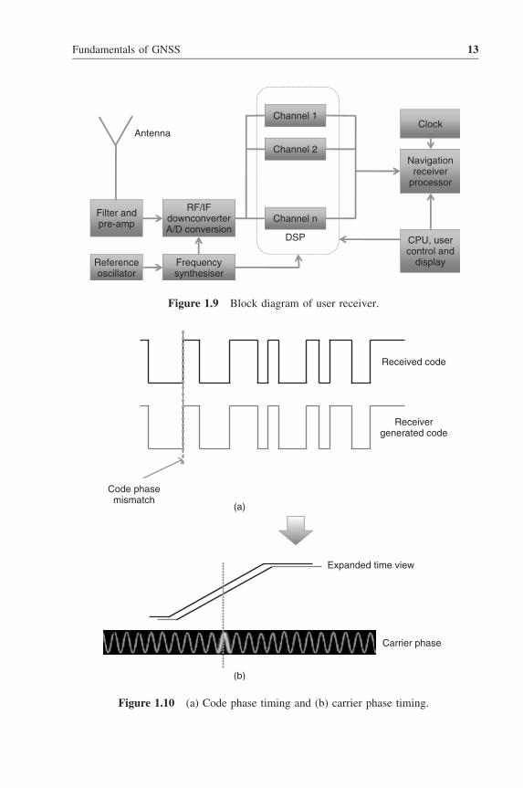
Fundamentals of GNSS 13
Antenna
Filter andpre-amp
Referenceoscillator
Frequencysynthesiser
RF/IFdownconverterA/D conversion
DSP CPU, usercontrol and
display
Channel 1
Channel 2
Channel n
Clock
Navigationreceiver
processor
Figure 1.9 Block diagram of user receiver.
(a)
Code phasemismatch
(b)
Expanded time view
Carrier phase
Receivergenerated code
Received code
Figure 1.10 (a) Code phase timing and (b) carrier phase timing.
14 Antennas for Global Navigation Satellite Systems
±10 ns, corresponding to a position error of ±3 m. This can be improved ifcarrier phase is used to give a finer timing for the received edge of the incomingpseudo-random code, as shown in Figure 1.10b. The receiver can measure thecarrier phase to about 1% accuracy by keeping a running count of the Dopplerfrequency shift of the carrier since satellite acquisition and the overall phasemeasurement contains an unknown number of carrier cycles, N , between thesatellite and the user. If this carrier cycle integer ambiguity can be determined,accuracies of the order of 1 mm can be achieved. The techniques employed bydifferential GPS (DGPS), described in the next section, aim to determine N .
GPS was originally a US military system and is still today administeredby the US DoD, which explains the background for the PPS and why theprecise P code can be encrypted so that only military equipment with a properdecryption key can access it. Here an additional code P is transmitted on L1 anda second on L2. In both cases the chip rate is 10.23 Mbits/s with a bandwidthof 20.46 MHz. The P code is pseudo-random and 37 weeks long but onlyabout 1 week is used. For protection against interfering signals transmittedby a possible enemy, the P code can be transmitted encrypted. During thisanti-spoofing (AS) mode the P code is encrypted by binary summing it witha slower rate pseudo-random noise code (W code) forming the so-called Ycode (called P(Y) mode) which requires a special key to extract the gold code.Even SPS was subject to ‘selective availability’, its role being to deny accuratepositioning to non-authorised users. This is achieved by dithering the satelliteclocks in a pseudo-random fashion to corrupt the range measurements, withauthorised users having a key to enable them to remove the dithering beforeprocessing. When enabled, the SPS location accuracy was limited to about100 m horizontally and about 150 m vertically, but in the year 2000 it waspermanently turned off.
Besides redundancy and increased resistance to jamming, the benefit of hav-ing two frequencies transmitted from one satellite is the ability to measuredirectly, and therefore remove, the ionospheric delay error for that satellite. Asthe ionosphere is a highly dynamic charged medium, its permittivity is alsodynamic and so the speed of light fluctuates by a small frequency-dependentamount, thus leading to positional errors. Ionospheric delay is one of the largestremaining sources of error in the GPS signal for a static receiver. Withoutsuch a two-frequency measurement, a GPS receiver must use a generic modelor receive ionospheric corrections from another source. As part of a generaldevelopment of NAVSTAR GPS the introduction of a second civilian signalchannel L2C was begun in 2006 (with the IIR-M satellites), which by about2016 will provide a 24-satellite constellation with this capability. In addition athird new civilian radio channel L5 has been allocated with a carrier frequency

Fundamentals of GNSS 15
of 1176.45 MHz (20.46 MHz bandwidth), which is in the Aeronautical RadioNavigation Service (ARNS) band authorised for use in emergencies and safetyof life applications. The first launch was in 2009 and the 24-satellite constella-tion with this capability will be achieved by about 2018. It is anticipated thatuse of the pilot carrier in this band combined with L1 will achieve improvedtracking in poor signal and multipath environments.
While most systems employ CDMA-based2 coding with BPSK modulation,Galileo uses binary offset carrier (BOC) modulation. BPSK has its spectralenergy concentrated around the carrier frequency, while BOC-modulated sig-nals have low energy around the carrier frequency and two main spectral lobesfurther away from the carrier (hence the name of split-spectrum modulation);this reduces the interference with BPSK and hence other GPS services.
1.4 Applications Including Differential GPS
The concept of local area differential GPS (LADGPS) is to place a GPS ref-erence receiver at a surveyed (known) location and to compute the differencesin latitude, longitude and geodetic height between the GPS measured positionand the known surveyed location. The GPS reference receiver is a survey-gradeGPS that performs GPS carrier tracking and can work out its own position toa few millimetres. For real-time LADGPS these differences are immediatelytransmitted to the local receivers by a low-frequency radio link (VHF or UHF)and they employ this data to correct their own GPS position solutions. Thisrequires that all the receivers make pseudo-range measurements to the sameset of satellites to ensure that errors are common. Where there is no need forreal-time measurement, such as in terrain mapping, the local receiver needsto record all of its measured positions and the exact time, satellite data, etc.,then post-processing the data along with that from the reference receiver yieldsthe required accurate locations. In both cases the basic measurement errors(or biases) related to each satellite measurement, such as ionospheric andtropospheric delay errors, receiver noise and clock offset, orbital errors, etc., canbe determined and corrected for. Table 1.2 [4] gives estimates of the pseudo-range error components from various sources in SPS mode. The total rms rangeerror is estimated at 7.1 m, and with LADGPS the error drops by a factor of 10.
Protocols have been defined for communicating between reference stationand remote users and one such is that from the Radio Technical Commissionfor Maritime Services (RTCM-104). The data rate is low (200 baud) and so
2 GLONASS originally used an FDMA-based system but is transferring to a CDMA-basedapproach.

16 Antennas for Global Navigation Satellite Systems
Table 1.2 GPS C/A code pseudo-range error budget (after [4])
Segment Error source GPS LADGPSsource 1 sigma error (m) 1 sigma error (m)
Space Satellite clock stability 1.1 0Satellite perturbations 1 0Broadcast ephemeris 0.8 0.1–0.6 mm/km*
User Ionospheric delay 7.0 0.2–4 cm/km*Tropospheric delay 0.2 14 cm/km*Receiver noise and
resolutions0.1 0.1
Multipath + others(interchannel bias etc.)
0.2 0.3
System Total (RSS) 7.1 0.3 m + 16 cm ×baseline in km
∗Baseline distance in km.RSS: Received Signal Strength.
can be transmitted to the remote receiver in a number of ways including aGPRS (General Packet Radio Service) mobile phone connection. The error inthe estimated corrections will be a direct function of the distance between thereference and remote receivers; it is possible to use a number of referencereceivers to provide a perimeter to the roving remote receiver [4].
As mentioned previously, the receiver can measure the carrier phase to about1% accuracy by keeping a running count of the Doppler frequency shift ofthe carrier since satellite acquisition by the receiver, but the overall phasemeasurement contains an unknown number of carrier cycles, N , between thesatellite and the user (Figure 1.11). The recording of this data over time canbe done at both the reference and roving receiver for the same set of satellitesat the same time. Combining this data in the form of interferometry leads toa set of equations over time that can be solved to determine the values of N(carrier cycle integer ambiguity) for each satellite received by the reference androving receivers. The corresponding code-phase-measured data can be used tolimit the size of the integer ambiguity to about ±10 λ to aid the solution. Abrute force solution to determining N could then be applied by calculating theleast squares solution for each time iteration and finding the minimum residual,but this is a large computational task (of the order of 300 000 residuals foreach time point for a ±10 λ ambiguity [4])! A better approach uses advanced

Fundamentals of GNSS 17
Earth surface
Satellite orbital track attimes t0 etc.
User
N + f1
N
N + f2
N + f3
t0
t1
t2 t3
Figure 1.11 Carrier phase as a function of time for a given satellite link.
processing techniques to choose suitable trial values for N [4] leading to 20 cmaccuracy in near real time and 1 mm accuracy with post-processing.
When millimetre accuracies are involved the location of the receive antenna’sphase centre is a vital component in achieving positional accuracy, as the phasecentre defines the point at which the electromagnetic energy is received by theantenna, and hence the location for the 3D point of measurement for GPS.The phase centre for an antenna is where the spherical phase fronts of the far-field radiation pattern of an antenna appear to emanate from in transmit mode.Since antennas are reciprocal devices, so long as they are isotropically passiveand linear this will also be the point at which the energy is received by theantenna. For a given antenna the phase centre is a function of the operatingfrequency and polarisation, and has a range of validity in terms of the solidangle surrounding the antenna boresight. The phase centre is easily determinedby far-field radiation pattern phase measurement as shown in Figure 1.12 fora set of planar pattern cuts for a given polarisation at different points aboutwhich the antenna is rotated. For a given operating frequency and polarisation,such measurements need to be undertaken in both the E plane and H planeto determine the 3D coordinates of the phase centre. The phase centre datais then referred to some fixed physical reference point on the antenna, suchdata normally being provided by the manufacturer for antennas to be used forprecision GPS.

18 Antennas for Global Navigation Satellite Systems
Measured phase
Z = Z1 Z = Z3
Z = Z2
Azi
mut
h an
gle
Transmit
Far-field antenna range
Phase centre is at Z = Z2 in this case.The phase centre position is often specifiedwith respect to the aperture or some othereasily identified physical point on the antenna
AUT mounted onturntable
Z
Move AUT with respect toturntable centre of rotationalong Z direction and recordphase pattern as a functionof angle
Figure 1.12 Antenna phase centre measurement. AUT: Antenna Under Test.
A key issue for high-precision measurements is the effect of multipath, wherea delayed version of the GPS signal is received by reflection from a nearbybuilding or the ground. Techniques to mitigate this include correlator designsto separate the multipath components, spectral techniques, multiple receiveantennas as well as sensible choice of site (where that is possible). Todaymultipath mitigation extends to mobile receivers in urban environments, andthe use of multiple antennas on vehicles is a possible solution.
Regional area and wide area DGPSs, as the names suggest, cover much widerareas and often use satellites to provide the differential data (e.g. the LEXfrequencies of the QZSS system in Table 1.1). Another significant applicationfor GPS is its use as a time standard, for example to synchronise master clocksin telecommunication systems.
References1. Hofmann-Wellenhof, B., Lichtenegger, H. and Wasle, E., GNSS – Global Navigation Satellite
Systems, GPS, GLONASS, Galileo and more, Springer, Vienna, 2008.

Fundamentals of GNSS 19
2. Engel, U., ‘Improving position accuracy by combined processing of Galileo and GPS satellitesignals’, Proceedings of the ISIF Fusion 2008 Conference, Cologne, Germany, 30 June–3 July 2008.
3. NAVISTAR-GPS Joint Programme Office, NAVSTAR-GPS user equipment: introduction, publicrelease version, February 1991.
4. Kaplan, E.D., Understanding GPS: Principles and applications , 2nd edn, Artech House,London, 2006.
5. MIT course web site ‘12.540 Principles of the Global Positioning System’. http://www-gpsg.mit.edu/˜tah/12.540/12.540_HW_01_soln.htm, last accessed on 23 December, 2011.

2Fundamental Considerationsfor GNSS Antennas
This chapter starts by describing radio wave propagation between a satellite anda ground receiver and the rationale for selecting circularly polarised (CP) waves.It also introduces the relevant propagation issues, such as multipath interferenceand the effects of ionospheric, tropospheric and RF interference, and coversfundamental issues in antenna design for GNSS applications. Finally, it presentsthe basic approaches for designing a CP antenna and highlights the technicalchallenges involved.
2.1 GNSS Radio Wave Propagation
Satellite navigation relies on signals carried by electromagnetic (EM) waves(radio waves). In order to design better GNSS antennas, we need to have agood understanding of radio wave propagation and related effects on satellitenavigation systems.
2.1.1 Plane Waves and Polarisation
A radio wave propagating over a long distance, as in a satellite navigationsystem, is always in the form of a plane wave. A plane EM wave is characterisedby having no field components in the propagation direction and the field onlyvarying in the propagation direction. A typical plane wave and its attributesare shown in Figure 2.1. The electric and magnetic fields are in phase and varysinusoidally along the propagation direction.
Antennas for Global Navigation Satellite Systems, First Edition.Xiaodong Chen, Clive G. Parini, Brian Collins, Yuan Yao and Masood Ur Rehman.© 2012 John Wiley & Sons, Ltd. Published 2012 by John Wiley & Sons, Ltd.

22 Antennas for Global Navigation Satellite Systems
Wavefront
l
Ex
Motion(Poynting vector/Propagation)
E0
x
y
zH0
Hy
λ2πWavenumber = k =
E = E0 cos (ωt – kz) x H = H0 cos (ωt – kz) y
Figure 2.1 Illustration of a plane EM wave.
The polarisation of a plane EM wave can be characterised as beinglinear, circular or elliptical, depending on the direction of its electric field vec-tor E = [Ex, Ey]. A constant direction of E characterises linear polarisation,as indicated in Figure 2.2a. A CP plane wave is characterised by the equalamplitude transverse components of the electric field, out of phase by 90◦.The electric field vector rotates along the propagation direction – tracing acircle on the x –y plane, as indicated in Figure 2.2b. When the two transversecomponents have different magnitudes or if the phase difference between themis different from 90◦, the electric field vector traces an ellipse on the x –y
plane, as shown in Figure 2.2c, and the polarisation is described as elliptical.Circular polarisation can be classified into right hand circular polarisation
(RHCP) and left hand circular polarisation (LHCP). An RHCP wave is definedas if the right hand thumb points in the direction of propagation, while thefingers curl along the direction of the E field vector rotation. It is consideredto be clockwise because, from the point of view of the source, looking in thedirection of propagation, the field rotates in a clockwise direction. An LHCPwave is defined as if the left thumb points in the direction of propagation whilethe fingers curl along the direction of the E field vector rotation. This conventionis also applied to elliptical polarisation. Different types of polarisations aresummarised in Figure 2.2.

Fundamental Considerations for GNSS Antennas 23
x
y
x
y
x-polarised y-polarised
x
y
x
y
Right Hand Left Hand
x
y
x
y
Left HandRight Hand
MajorMinor
(a)
(b)
(c)
Figure 2.2 Different types of plane wave polarisations: (a) Linear polarisation,(b) Circular polarisation and (c) Elliptical polarisation.
When a plane radio wave propagates in a homogeneous medium, it has aconstant velocity and remains in its original polarisation. However, the radiowave will experience many changes in its attributes when propagating throughdifferent media, as it does in the case of satellite navigation systems.
2.1.2 GNSS Radio Wave Propagation and Effects
The radio wave transmitted from a moving GNSS satellite propagates throughthe atmosphere (ionosphere and troposphere) and reaches the ground receiver,as shown in Figure 2.3. It encounters several impairments, such as attenuation,Doppler shift, propagation delay in the ionosphere and troposphere, multipathand interference. The link budget between a satellite and a ground stationmust take into account the attenuations caused by distance, and the effects ofabsorption and scattering in the ionosphere and troposphere. Other impairments

24 Antennas for Global Navigation Satellite Systems
Ionosphere
Troposphere Local
~10 km
Figure 2.3 Radio wave propagation between a GNSS satellite and a ground receiver.
cause navigation errors. Together with their associated mitigation methods,these are discussed briefly below.
2.1.2.1 Doppler Shift
The Doppler shift is caused by the well-known physical fact that relative motionbetween a transmitter and receiver will cause a perceived frequency shift in thereceived signal. An approaching transmitter increases the received frequency,whereas a receding transmitter decreases it. In satellite navigation, a Dopplershift of about 5 kHz maximum is created by satellite motion when the satelliteis moving directly towards or away from the receiver. Motion of the receiveralso creates a small Doppler shift at a rate of 1.46 Hz/km/h. Taking into accountreceiver oscillator frequency offset, the total maximum frequency uncertaintyat the receiver is roughly ±10 kHz. The receiver must search in this 20 kHzband to find detectable GNSS signals [1]. Within this band each satellite willhave its own characteristic Doppler shift according to its orbital characteristicsand the position of the receiver.
2.1.2.2 Effects of the Ionosphere
The ionosphere is a layer of electrons and charged atoms and molecules (ions)that surround the Earth, stretching from a height of 50 to 1000 km. The iono-sphere can be characterised by its total electron content (TEC). The TEC isinfluenced by solar activity, diurnal and seasonal variations, and the Earth’s

Fundamental Considerations for GNSS Antennas 25
magnetic field. Radio waves travelling through the ionosphere can undergo achange in their polarisation, which is known as Faraday rotation. This effectmay cause linearly polarised (LP) radio waves to become elliptically or circu-larly polarised. The major effect of the ionosphere on a GNSS signal is thefrequency-dependent phase shift (group delay), caused by the dispersive char-acteristics of the ionosphere. We can reduce the effect of ionospheric dispersionby employing two widely spaced frequencies. By employing a diversity schemeat the receiver, we can correct almost all the ionospheric effects. It is for thisreason that GPS satellites transmit signals at two carrier frequencies, L1 at1575.42 MHz and L2 at 1227.60 MHz.
2.1.2.3 Effects of the Troposphere
The troposphere, extending from the Earth’s surface to a height of about 50 km,is non-dispersive at GNSS frequencies. The troposphere delays radio wavesby refraction. The reasons for the refraction are different concentrations ofwater vapour in the troposphere, caused by different weather conditions. Theresulting error is smaller than the ionospheric error, but it cannot be eliminatedby calculation. It can only be approximated by a general calculation model.
2.1.2.4 Multipath Propagation
Multipath propagation occurs when the receiver picks up signals from the orig-inating satellite that have travelled by more than one path. Multipath is mainlycaused by reflecting surfaces near the receiver. In the example in Figure 2.3,the satellite signal arrives at the receiver through three different paths, onedirect and two reflected. As a consequence, the received signals have relativephase offsets, which results in pseudo-range error. The range error caused bythe multipath may grow to about 100 m in the vicinity of buildings [1]. Themethods of mitigating multipath effects can be classified as (i) antenna basedand (ii) signal processing based. One of the antenna-based approaches is toimprove the antenna radiation pattern by using choke rings to suppress signalsreceived from directions below the horizon. Another approach is to choosean antenna that takes advantage of the radio wave polarisation. If transmittedGNSS signals are right-handed circularly polarised, then after one reflectionthe signals are left-handed polarised. So if the receiver antenna is designed tobe right hand polarised, it will reject many reflected multipath signals. Signalprocessing methods for mitigating multipath have recently progressed substan-tially [1]; however, even with high-performance correlator receivers, multipatherrors still occur frequently.
26 Antennas for Global Navigation Satellite Systems
We have only discussed radio wave propagation in a general environment.Nowadays, GPS receivers are often integrated with mobile phone handsets.Radio wave propagation is more complicated in this scenario, in which weneed to consider the effects of the human body and the mobile terminal.
2.1.3 Why CP Waves in GNSS?
Having discussed radio wave propagation and its impairments in the previoussection, we can easily see the benefits of employing CP waves in satellitenavigation (RHCP in GNSS).
Firstly, a CP radio wave enhances the polarisation efficiency of the receiv-ing antenna. Maximising the received signal using LP or elliptically polarised(EP) antennas requires the receiving antenna to be correctly aligned relative tothe direction of propagation. Using RHCP antennas at the satellite and at thereceiver means that no polarisation alignment is needed. Secondly, a CP waveis capable of combating Faraday rotation in the ionosphere. If an LP wave isadopted, the signal becomes EP or even CP after passing through ionosphere,so an LP antenna on the receiver can only pick up a fraction of the incomingsignal. Thirdly, a CP radio wave can be utilised to reject multipath signals. Asmentioned earlier, a right hand polarised signal becomes left hand polarisedafter reflection from a surface. An RHCP receiving antenna would reject thesereflected signals.
The design of a CP antenna is more complicated and difficult compared withthat of an LP antenna, especially in GNSS applications. Thus this text providescomprehensive coverage of this topic.
2.2 Antenna Design Fundamentals
An antenna can be regarded as a transducer between EM waves travelling infree space and guided EM waves in RF circuits [2]. Antennas are characterisedby a number of parameters and can be classified into a number of differentcategories.
2.2.1 Antenna Fundamental Parameters
In the design of antennas, a number of fundamental parameters must be spec-ified. These key parameters are reviewed in the following subsections.

Fundamental Considerations for GNSS Antennas 27
2.2.1.1 Impedance Bandwidth
We may define impedance bandwidth as the frequency range over which 90%of the incident power is delivered to the antenna – the reflection coefficientS11 < −10 dB and the voltage standing wave ratio (VSWR) is less than 2:1.The absolute impedance bandwidth can be calculated as the difference betweenthe upper and lower frequencies at which these criteria are met. Alternatively,the fractional impedance bandwidth can be calculated as the percentage of theupper and lower frequency difference divided by the centre frequency of thebandwidth:
BW = fmax − fmin
fcentre× 100% (2.1)
2.2.1.2 Radiation Pattern
The radiation pattern is a graphical representation of the radiation characteristicsof the antenna as a function of spatial coordinates. For a small antenna it isgenerally determined in the far-field region and is represented as a functionof directional coordinates. Spherical coordinates are typically used, where thex –z plane (measuring θ with fixed ϕ at 0◦) is called the elevation plane andthe x –y plane (measuring θ with fixed ϕ at 90◦) is called the azimuth plane,as shown in Figure 2.4a.
Figure 2.4b illustrates an example of an antenna scalar radiation pattern [3].Its major features are as follows:
• Major lobe or main beam: The part that contains the direction of maximumradiation. The direction of the centre of an essentially symmetrical mainbeam is called the electrical boresight of an antenna.
• Back lobe: A radiation lobe that is directly opposite to the main lobe. Backlobes may refer to any radiation lobes between 90◦ and 180◦ from the bore-sight direction.
• Minor lobes: Any lobe apart from the main beam.• Half-power beamwidth (HPBW): The angle subtended by the half-power
points of the main lobe.
2.2.1.3 Antenna Phase Centre
As discussed in Chapter 1, antenna phase centre is a concept related to thephase pattern, that is the equiphase surfaces of an antenna, shown as dashed

28 Antennas for Global Navigation Satellite Systems
(a) (b)
(c)
Main lobe maximum direction
Main lobe
Minorlobes
Half-power point (right)Half-power point (left)
Half-power beamwidth (HP)
Beamwidth between first nulls (BWFN)
0.5
1.0
xy
zr0
z
y
x
r
r
f
f
ˆˆ
ˆ
Figure 2.4 (a) Spherical coordinates, (b) an example of a radiation pattern and (c) thephase pattern (equiphase surfaces) of an antenna on an azimuth plane.
lines on a particular azimuth plane in Figure 2.4c. In the far-field region, theequiphase surface is close to a spherical surface, indicated as the outermostcircle in Figure 2.4c. The centre of the sphere is the equivalent phase centre ofthe antenna.
In most cases of antenna design, we are only concerned with the scalarradiation pattern, the spatial distribution of the field strength. However, insatellite surveying and other precision measurements, the phase of the receivedsignal is used to obtain a greater precision of position, so the antenna phasecentre and its characteristics need to be taken into account.
2.2.1.4 Directivity and Gain
The directivity of a receiving antenna is the ratio of the sensitivity to signalsarriving from the direction of the maximum of the main lobe to the meansensitivity to signals arriving from all directions in 3D space.
The gain of a receiving antenna is the ratio of the signal received by theantenna compared with that received by a lossless isotropic antenna in thesame signal environment.

Fundamental Considerations for GNSS Antennas 29
2.2.1.5 Efficiency
Total antenna efficiency describes the losses incurred in the process of convert-ing the input power to radiated power:
Total efficiency = radiation efficiency × reflection efficiency
Radiation efficiency takes into account conduction and the dielectric losses(heating) of the antenna. Reflection (mismatch) efficiency accounts for thepower loss due to impedance mismatch.
2.2.1.6 Polarisation
As mentioned earlier, polarisation can be described as the property of theEM waves that defines the directional variation of the electric field vector.The polarisation of a receiving antenna may be defined by reference to thepolarisation of an incoming wave of a given field strength for which the antennadelivers maximum received power.
Generally speaking, the polarisation of a receiving antenna is not the sameas the polarisation of the incident wave. The polarisation loss factor (PLF)characterises the loss of received power due to polarisation mismatch .
Antennas can be classified in accordance with their polarisation characteris-tics as LP, CP and EP.
For an EP antenna, there is an additional characteristic – the axial ratio (AR)defined as the ratio of the major axis to the minor axis of the polarisation ellipse,as shown in Figure 2.2c:
AR = major axis
minor axis(2.2)
The AR is unity (0 dB) for a perfect CP antenna. In practice, when the AR isless than 3 dB, the antenna is usually accepted as a CP antenna.
2.2.2 LP Antenna Design and Example
The LP antenna usually has a simple structure, such as a dipole, which we useas a straightforward example to illustrate the characteristics of an LP antenna.
A half-wavelength dipole antenna working at the GPS L1 band is shown inFigure 2.5. The length of the dipole is approximately λ/2, so since the centralfrequency is 1575.42 MHz, l = 95.2 mm. The antenna illustrated is LP in thevertical direction.

30 Antennas for Global Navigation Satellite Systems
l
Figure 2.5 Schematic of an ideal dipole.
1400 1500 1575.42 1600 1700–20
–15
–10
–5
0
Frequency (MHz)
S11
(dB
)
Figure 2.6 Simulated S11 curve of a half-wavelength dipole.
The dipole antenna is modelled by using CST Microwave Studio [4].Figure 2.6 shows the simulated S11 for the antenna. The antenna performswell in the L1 frequency band with a −10 dB bandwidth of 153 MHz.
The radiation patterns of the dipole antenna in the elevation and azimuthplanes are illustrated in Figure 2.7. The pattern in the azimuth plane is a circle,indicating that the dipole is an omnidirectional antenna. The pattern in theelevation plane indicates the major lobe is directed towards the horizontal axis(θ = 90◦) with a directivity of 2.14 dB and with a 3 dB beamwidth of 78◦. Apractical dipole will be discussed again in Chapter 6.

Fundamental Considerations for GNSS Antennas 31
Elevation plane
Azimuth planeq = 90°
f = 90°
EH
Figure 2.7 The 2D radiation pattern of a half-wavelength dipole.
2.3 CP Antenna Design
As we mentioned earlier, CP antennas are required for optimum reception ofGNSS signals. We will cover CP antenna design issues in this section.
2.3.1 CP Antenna Fundamentals and Types
CP antennas can be realised in design through different structures and feedingtechniques. In terms of structures, CP antennas can be classified into helical,spiral and microstrip patch types.
2.3.1.1 Helical Antennas
A helical antenna can easily generate circular polarisation since the currentfollows a helical path like the CP EM wave. In practice, it comprises a helixwith a ground plane, where a clockwise winding provides RHCP and anti-clockwise provides LHCP. An example is shown in Figure 2.8.
The geometry of a helix consists of N turns, diameter D and spacing S
between turns, as shown in Figure 2.8. The axial (endfire) mode is usually usedto achieve circular polarisation over a wide bandwidth. To excite this mode, thediameter D and spacing S must be large fractions of the wavelength. In practice,the circumference of the helix must be in the range of 3/4 < πD/λ < 4/3 and

32 Antennas for Global Navigation Satellite Systems
D
S
Figure 2.8 Helical antenna geometry.
the spacing about λ/4. Most often the helix is fed by a coaxial line and issupported by a ground plane with a diameter of at least λ/2.
The helix provides high gain and broad bandwidth, but is large in size, so it isnormally used as a transmitting antenna on a satellite, or as a high-gain receiv-ing antenna. One variation of the helix, the quadrifilar helix, can be made incompact form. Thus it has also been employed on the receiving terminals. Thefeatures of the quadrifilar antenna will be addressed in the following chapters.
2.3.1.2 Spiral Type
Flat spiral antennas belong to the class of frequency-independent antennaswhich operate over a wide range of frequencies. Figure 2.9 shows a typicalconfiguration of a two-arm flat spiral antenna. The lowest frequency of opera-tion occurs when the total arm length is comparable with the wavelength. Forall frequencies above this and below a frequency defined by the extent to whichthe spiral geometry is maintained near the central feed point, the pattern andimpedance characteristics are sensibly frequency independent. Spiral antennasare inherently CP, with low gain. Lossy cavities are usually placed behind thespiral to eliminate back lobes, because the structure is intrinsically bidirectional,while a unidirectional pattern is usually preferred. Spiral antennas are classified

Fundamental Considerations for GNSS Antennas 33
Figure 2.9 A two-arm log-spiral antenna backed with a cavity.
into different types: Archimedean spiral, square spiral, log spiral, etc. [2]. Atypical cavity-backed two-arm log-spiral antenna is shown in Figure 2.9.
Different designs of spiral antenna can be obtained by varying the number ofturns, the spacing between turns and the width of the arms. The properties ofthe antenna also depend on the permittivity of the dielectric medium on whichthe spiral is supported.
The antenna comprises usually two conductive spiral arms, extending out-wards from the centre. The antenna may be a flat disc, with conductors resem-bling a pair of loosely nested clock springs, or the spirals may extend in a 3Dshape like a tapered screw thread (a conical spiral). The direction of rotation ofthe spiral, as viewed from behind, defines the sense of polarisation. Additionalspirals may be included to form a multi-spiral structure.
2.3.1.3 Patch Antennas
To understand how a patch CP antenna works, we need to see how a microstrippatch antenna operates. A simple rectangular patch antenna can be viewed as adielectric-loaded cavity, having various resonant modes. The fundamental modeis the TMx
010 mode, as shown in Figure 2.10a. The equivalent magnetic currentis shown in Figure 2.10b. The currents flowing along the y-direction (sides2 and 4) cancel each other, while the currents flowing along the x-direction(sides 1 and 3) add. So the net exciting current in the TMx
010 mode flows in thex-direction. The other fundamental mode of a patch cavity is the TMy
010 mode

34 Antennas for Global Navigation Satellite Systems
(a) (b)
(2)
(3)
(4)
(1)
TMx010
W
L
h
Figure 2.10 (a) Patch cavity mode, TMx010, and (b) equivalent magnetic current flows.
in the y-direction, similar to the patterns in Figure 2.10, but rotated by 90◦.The net exciting current in TMy
010 mode flows in the y-direction.In a square patch antenna, the TMx
010 and TMy
010 modes have the sameresonant frequency, so if we excite these two modes simultaneously with a90◦ time–phase difference, a CP wave can be launched. A similar analysis canbe applied to a circular patch antenna which supports the fundamental TM110mode in both the x- and y-directions.
Basically, there are two feeding approaches to achieve CP on a patch antenna:
1. Dual-fed CP patch antenna: In this design, two feed ports are excited withorthogonal currents having 90◦ phase difference. For a square patch antenna,the ideal method is to feed the patch at the centre of two adjacent edges.A power divider or 90◦ hybrid can be used to obtain the quadrature phasedifference between the feeds. Another method is to use offset feeding whereone feed line is one quarter wavelength longer than the other. Figure 2.11shows two different types of dual feeding.
2. Single-fed CP patch antenna: The antenna is fed at a single point wherethe generated mode is separated into two orthogonal modes by the effectof an offset feed point together with geometrical perturbations of the patchsuch as slots or truncations on its edges or corners, as shown in Figure 2.12.The radiated fields excited by these two generated modes are orthogonallypolarised with equal amplitude, and are 90◦ out of phase at the centre fre-quency when the perturbed segment is optimally adjusted. This arrangementenables the antenna to act as a CP radiator despite being fed only at a singlepoint. This antenna has several advantages over the dual-fed ones, such as

Fundamental Considerations for GNSS Antennas 35
no need for an external feed network and its compact size. However, theAR bandwidth of a patch antenna of this type is normally smaller than thatof a dual-fed patch and is only suitable for coverage of one of the GNSSfrequency bands.
There are other types of CP patch antennas, such as pentagonal, triangularand elliptical patches and composite CP antennas [4]. Also, various variationsof CP patch antennas have been designed in practical GNSS applications. Thesepractical patch antenna designs will be discussed in the following chapters.
2.3.2 Simple CP Antenna Design Example
Here we design a corner-truncated square patch CP antenna to cover the GPSL1 band to demonstrate CP antenna characteristics.
The geometry of the probe-fed truncated corner square patch antenna isshown in Figure 2.13.
The optimised dimensions of the antenna are Lp = 53.4 mm, Ls = 100 mm,a = 49.9 mm, �a = 3.5 mm, b = 26.7 mm and c = 16 mm. An FR4 dielectric
F1
F2
F1
F2
Power divider
Squarepatch
λ/4
Figure 2.11 Dual-feed types of circularly polarized antenna [5]. Reproduced withpermission from IET.
F F
Figure 2.12 Singly fed types of CP patch antennas [5]. Reproduced with permissionfrom IET.
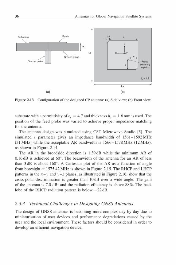
36 Antennas for Global Navigation Satellite Systems
Coaxial probe
Ground plane
Substrate Patch
hs
Ls
Ls
Δa a
c
bProbe
soldering to patch
X
Z
Y
∋
r = 4.7
(b)(a)
Figure 2.13 Configuration of the designed CP antenna: (a) Side view; (b) Front view.
substrate with a permittivity of εr = 4.7 and thickness hs = 1.6 mm is used. Theposition of the feed probe was varied to achieve proper impedance matchingfor the antenna.
The antenna design was simulated using CST Microwave Studio [5]. Thesimulated s parameter gives an impedance bandwidth of 1561–1592 MHz(31 MHz) while the acceptable AR bandwidth is 1566–1578 MHz (12 MHz),as shown in Figure 2.14.
The AR in the broadside direction is 1.39 dB while the minimum AR of0.16 dB is achieved at 60◦. The beamwidth of the antenna for an AR of lessthan 3 dB is about 160◦. A Cartesian plot of the AR as a function of anglefrom boresight at 1575.42 MHz is shown in Figure 2.15. The RHCP and LHCPpatterns in the x –y and y –z planes, as illustrated in Figure 2.16, show that thecross-polar discrimination is greater than 10 dB over a wide angle. The gainof the antenna is 7.0 dBi and the radiation efficiency is above 88%. The backlobe of the RHCP radiation pattern is below −22 dB.
2.3.3 Technical Challenges in Designing GNSS Antennas
The design of GNSS antennas is becoming more complex day by day due tominiaturisation of user devices and performance degradations caused by theuser and the local environment. These factors should be considered in order todevelop an efficient navigation device.

Fundamental Considerations for GNSS Antennas 37
1400 1500 1575.42
(a)
1600 1700–20
–15
–10
–5
0
Frequency (MHz)
S11
(d
B)
(b)
10
1500 1560 1575.421570 1580 15900
3
2
4
6
8
Frequency (MHz)
Axi
al R
atio
(d
B)
Figure 2.14 Reflection coefficient and AR plots of the CP antenna.

38 Antennas for Global Navigation Satellite Systems
20
15
10
Axi
al R
atio
(d
B)
5
0–180 –120 –60 0 60
Theta (degrees)120 180
Figure 2.15 Cartesian plot of AR in x –y plane at 1575.42 MHz.
Z
YY X
X
Y
X
RHCPLHCP
(a) (b)
10
30
210
60
240
90
270
120
300
150
330
180 0–40–30 –20 –10 0 10
30
210
60
240
90
270
120
300
150
330
180 0–40–30 –20 –10 0
Figure 2.16 Radiation pattern RHCP (solid curve) and LHCP (dot–dashed curve) at1575.42 MHz: (a) x –y Plane; (b) y –z Plane.

Fundamental Considerations for GNSS Antennas 39
2.3.3.1 Limitation on the Size and Shape of Antennas
A major technical challenge comes from the limitation on the size and shape ofantennas when adding GNSS functions to small devices such as mobile handsetsand personal trackers. As the size of average mobile handsets continues to fall,the space for installing the GPS antenna on the PCB is really limited. Tocombat this challenge, the majority of GPS antennas on mobile phones are ofthe space-saving LP type, in the form of PIFAs (Planar Inverted-F Antennas) orIFAs (Inverted-F Antennas). In order to compensate the lower effective antennagain of an LP antenna, a low-noise amplifier (LNA) is usually used togetherwith the antenna. Though CP patch antennas, usually on a high-permittivityceramic substrate, are still employed in some handsets, studies have shown thatthe advantage of a CP antenna disappears in a complex operating environmentwith rich multipath [6]. This issue is further addressed in the following chapters.
2.3.3.2 Multiband and Broadband Operation
With the development of integrated GNSS receivers covering GPS, GLONASS,Galileo and the Chinese Compass systems, there is a demand for multibandor broadband CP receiving antennas. This demand poses another challenge indesigning antennas for compact GNSS receivers since small CP antennas areusually narrow band. Considerable research work has been carried out in thisarea and different approaches have been proposed to meet such a demand. Thisis the main topic of Chapter 5.
2.3.3.3 The Effects of the Environment, Human Body and Platform
The performance of a GNSS antenna on a mobile terminal is affected substan-tially by its surroundings. Firstly, the antenna will pick up multipath signalsdue to reflections, refractions and scattering of incident radio waves in clut-tered environments, such as city streets and indoors. These multipath signalshave arbitrary polarisation and can cause substantial positioning errors. Sec-ondly, the antenna is greatly affected by the human body in its vicinity. Itis well known that the human body, being a lossy medium, can reduce theradiation efficiency of an antenna, degrade its radiation pattern and detune theimpedance matching at its feed point. Finally, other components on the mobileplatform can also affect GNSS antenna performance, distorting the radiationpattern, reducing gain and causing EM interference. These effects and relevantmitigation measures are the main topics in Chapters 6, 7 and 8.

40 Antennas for Global Navigation Satellite Systems
2.3.3.4 EM Interference
EM interference can be categorised as intentional and unintentional interfer-ence. Any intentional interference is unlawful, but GNSS receivers for somepurposes, for example military and law enforcement applications, must be ableto function in its presence. Sources of unintentional interference include out-of-band emissions from other services and in-band emissions, in particularfrom other GNSS systems. Spread-spectrum GNSS signals reduce the effect ofnarrowband interfering signals. Interference can be further mitigated by usingadaptive antenna and filter designs to filter the signal in the spatial, time andfrequency domains. On a mobile platform, EM interference may be emittedfrom other components or devices. It is challenging to isolate and mitigate thistype of EM interference in designing a mobile platform. Further discussion ofthis issue is provided in Chapter 8.
2.3.3.5 Other Issues
There are other issues to be considered in the design of GNSS antennas forvarious applications. For example, in the high-precision positioning service(differential GPS), stability of the phase centre of the antenna is required.This imposes another constraint in the design of GNSS antennas. This issue isaddressed in the following chapters.
References1. Van Diggelen, F., A-GPS: Assisted GPS, GNSS, and SBAS , Artech House, London, 2009.2. Balanis, C.A., Antenna Theory: Analysis and Design , 2nd edn, John Wiley & Son, Inc.,
New York, 1997.3. Stutzman, W.L. and Thiele, G.A., Antennas Theory & Design , John Wiley & Sons, Ltd,
Chichester, 1981.4. CST Microwave Studio, User Manual , 2009.5. James, J.R. and Hall, P.S., Handbook of microstrip antennas , Peter Peregrinus, London, 1989.6. Pathak, V., Thornwall, S., Krier, M. et al ., ‘Mobile handset system performance comparison
of a linearly polarized GPS internal antenna with a circularly polarized antenna’, Proceedingsof IEEE Antennas and Propagation Society International Symposium 2003, Columbus, OH,June 22–27, 2003, Vol. 3, pp. 666–669.

3Satellite GNSS Antennas
3.1 Navigation Antenna Requirements
This chapter will take an overview of the antenna requirements and designtechniques used for the spacecraft segment of the GPS system. Although theantenna farms are complex high-value systems, the antenna designer can inferuseful techniques that can be translated into constructing specialised GNSSuser antennas. Figure 3.1 shows the level of complexity of an antenna farm forthe GPS III satellite. A typical spacecraft antenna farm consists of a numberof antenna systems including:
• L-band downlink array that provides the L1, L2 and L5 navigation signals.• UHF uplink array for search and rescue.• S-B and TT&C (Tracking Telemetry & Control) up- and downlinks.• UHF antennas for satellite control.
Here we will concern ourselves with the first two that are specific to GNSSantenna design.
3.2 Types of Antenna Deployed
As an example of a modern navigation antenna array we will consider thedesign for Galileo. Table 3.1 summarises the specification.
This performance is achieved by using a 1.4 m diameter planar array of45 stacked patch antenna elements forming six triangular subarrays, as shown inFigure 3.2 [1]. There are two types of subarray (type A = six elements and typeB = nine elements) and they are placed alternatively in a radial pattern around
Antennas for Global Navigation Satellite Systems, First Edition.Xiaodong Chen, Clive G. Parini, Brian Collins, Yuan Yao and Masood Ur Rehman.© 2012 John Wiley & Sons, Ltd. Published 2012 by John Wiley & Sons, Ltd.
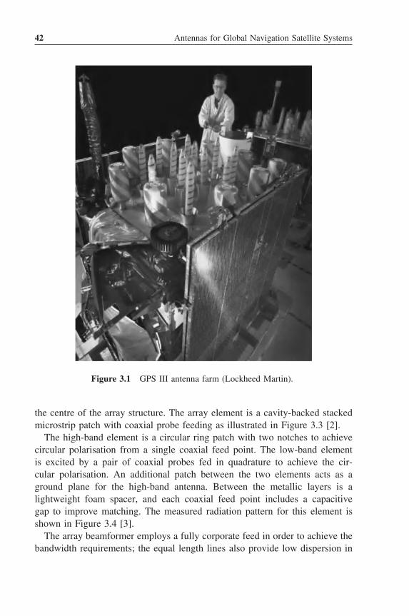
42 Antennas for Global Navigation Satellite Systems
Figure 3.1 GPS III antenna farm (Lockheed Martin).
the centre of the array structure. The array element is a cavity-backed stackedmicrostrip patch with coaxial probe feeding as illustrated in Figure 3.3 [2].
The high-band element is a circular ring patch with two notches to achievecircular polarisation from a single coaxial feed point. The low-band elementis excited by a pair of coaxial probes fed in quadrature to achieve the cir-cular polarisation. An additional patch between the two elements acts as aground plane for the high-band antenna. Between the metallic layers is alightweight foam spacer, and each coaxial feed point includes a capacitivegap to improve matching. The measured radiation pattern for this element isshown in Figure 3.4 [3].
The array beamformer employs a fully corporate feed in order to achieve thebandwidth requirements; the equal length lines also provide low dispersion in
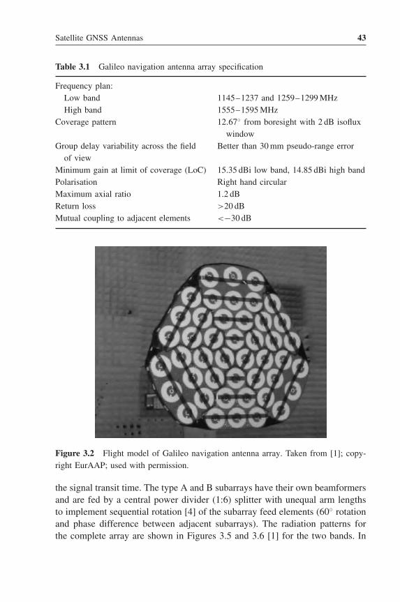
Satellite GNSS Antennas 43
Table 3.1 Galileo navigation antenna array specification
Frequency plan:Low band 1145–1237 and 1259–1299 MHzHigh band 1555–1595 MHz
Coverage pattern 12.67◦ from boresight with 2 dB isofluxwindow
Group delay variability across the fieldof view
Better than 30 mm pseudo-range error
Minimum gain at limit of coverage (LoC) 15.35 dBi low band, 14.85 dBi high bandPolarisation Right hand circularMaximum axial ratio 1.2 dBReturn loss >20 dBMutual coupling to adjacent elements <−30 dB
Figure 3.2 Flight model of Galileo navigation antenna array. Taken from [1]; copy-right EurAAP; used with permission.
the signal transit time. The type A and B subarrays have their own beamformersand are fed by a central power divider (1:6) splitter with unequal arm lengthsto implement sequential rotation [4] of the subarray feed elements (60◦ rotationand phase difference between adjacent subarrays). The radiation patterns forthe complete array are shown in Figures 3.5 and 3.6 [1] for the two bands. In
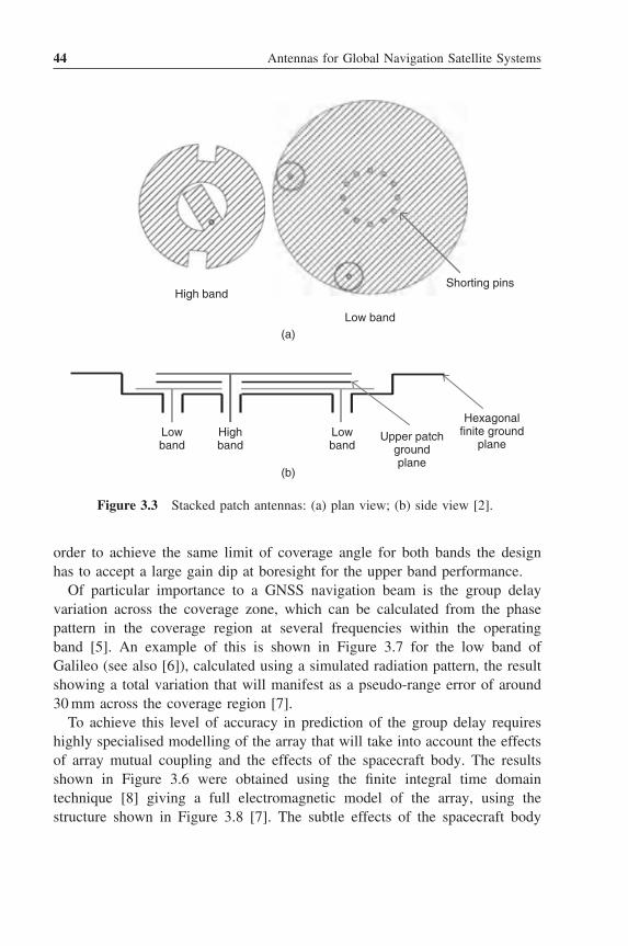
44 Antennas for Global Navigation Satellite Systems
Low band
High band
(a)
(b)
Lowband
Lowband
Highband
Upper patchgroundplane
Hexagonalfinite ground
plane
Shorting pins
Figure 3.3 Stacked patch antennas: (a) plan view; (b) side view [2].
order to achieve the same limit of coverage angle for both bands the designhas to accept a large gain dip at boresight for the upper band performance.
Of particular importance to a GNSS navigation beam is the group delayvariation across the coverage zone, which can be calculated from the phasepattern in the coverage region at several frequencies within the operatingband [5]. An example of this is shown in Figure 3.7 for the low band ofGalileo (see also [6]), calculated using a simulated radiation pattern, the resultshowing a total variation that will manifest as a pseudo-range error of around30 mm across the coverage region [7].
To achieve this level of accuracy in prediction of the group delay requireshighly specialised modelling of the array that will take into account the effectsof array mutual coupling and the effects of the spacecraft body. The resultsshown in Figure 3.6 were obtained using the finite integral time domaintechnique [8] giving a full electromagnetic model of the array, using thestructure shown in Figure 3.8 [7]. The subtle effects of the spacecraft body

Satellite GNSS Antennas 45
0
Theta (degrees)
–5
–10
–15
–20
–25
–30
–35
–40
–45
–50–80 –60 –40 –20 200 40 60 80
E-f
ield
(dB
)
Figure 3.4 Measured co-polar and cross-polar radiation pattern for isolated elementat 1228 MHz (for a number of phi cuts). Taken from [3]; copyright EurAAP; used withpermission.
can be seen in Figure 3.9 where the edges of coverage gain levels are plottedboth with the array in isolation and mounted on the spacecraft body model ofFigure 3.8. Such a model required up to 7 million mesh cells with run timesof the order of 24 hours.
Such a process is acceptable for final performance evaluation, but not suitableas a design process. The approach was to undertake a full wave simulation ofthe isolated array element including its ground plane; a generalised scatteringmatrix (GSM) of each element is then obtained using coaxial and sphericalmodal expansions from a hybrid 3D finite element modal analysis. The GSMsof the array elements are analytically connected by rotating and translatingspherical modes to obtain the GSM for the whole array. This brings the mod-elling time down to a few minutes per frequency point, which is much moresuitable for the design process; details of the analytical method can be foundin [4]. It is essential to realise that, to achieve the level of modelling accu-racy required, particularly in determining the accurate mutual coupling effect,an accurate model of the beam-forming network (BFN) must be achieved sothat each array antenna element is terminated in the true complex impedance

46 Antennas for Global Navigation Satellite Systems
(a)
(b)
0
Theta (degrees)
10
–10
–20
–30
–40–80 –60 –40 –20 20
20
0 40 60 80
CP
Gai
n (d
B)
Theta (degrees)
15
14
13
12–5–10–15 0 5 10 15
CP
Gai
n (d
B)
16
17
18
Figure 3.5 Co- and cross-polar gain radiation pattern for the low band (1237 MHz)for various phi cuts: (a) full pattern; (b) expanded region of coverage area. Taken from[1]; copyright EurAAP; used with permission.

Satellite GNSS Antennas 47
(a)
(b)
0
Theta (degrees)
10
–10
–20
–30
–40–80 –60 –40 –20 20
20
0 40 60 80
CP
Gai
n (d
B)
Theta (degrees)
15
14
13
12–5–10–15 0 5 10 15
CP
Gai
n (d
B)
16
17
18
Figure 3.6 Co- and cross-polar gain radiation pattern for the high band (1575 MHz)for various phi cuts: (a) full pattern; (b) expanded region of coverage area. Taken from[1]; copyright EurAAP; used with permission.

48 Antennas for Global Navigation Satellite Systems
Phi angle around boresight (degrees)
5
0 50 100 150 200 250 300 350
Bor
esig
ht a
ngle
(de
gree
s)
0
10
15
Figure 3.7 Simulated group delay (pseudo range in mm) for the 1150–1220 MHzband. Taken from [7]; copyright EurAAP; used with permission.
Figure 3.8 Galileo navigation array on spacecraft body model. Taken from [7]; copy-right EurAAP; used with permission.
presented to it by the BFN. Details of the method employed for Galileo can befound in [6].
Helical arrays are a very popular choice of antenna for spacecraft and indeedthe Sputnik satellite in 1957 brandished a helical antenna [9]. The use of helical

Satellite GNSS Antennas 49
15
15.2
15.4
15.6
15.8
16
–180 –120 –60 0 60 120 180
Phi (degrees)
Edg
e of
cov
erag
e ga
in (
dB)
(a)
15
15.2
15.4
15.6
15.8
16
–180 –120 –60 0 60 120 180
Phi (degrees)
Edg
e of
cov
erag
e ga
in (
dB)
(b)
Figure 3.9 Edge of coverage gain value for 1220 MHz: (a) on infinite ground plane;(b) on spacecraft body model of Figure 3.8. Taken from [7]; copyright EurAAP; usedwith permission.

50 Antennas for Global Navigation Satellite Systems
Figure 3.10 Galileo search and rescue helical antenna array on spacecraft body model.Taken from [7]; copyright EurAAP; used with permission.
antennas in space reflects their high gain, ease of fabrication and ease of gen-eration of circular polarisation, details of which are given in Chapter 2.
Here we consider the Galileo search and rescue array antenna operating at400 MHz, a spacecraft model of which is shown in Figure 3.10 [7] and aprototype photograph in Figure 3.11. Because of the 3D curved structure ofthe helical antenna modelling, using a rectangular grid for the finite integraltime domain technique requires very small cell sizes (λ/40). Again the effectof the spacecraft body model, rather than an infinite ground plane, influencedthe edge of coverage gain pattern by as much as 0.3 dB [7].
3.3 Special Considerations for Spacecraft Antenna Design
3.3.1 Passive Intermodulation Effects
It is essential that all transmit antennas on board a spacecraft do not interferewith other receivers via the process of passive intermodulation (PIM). Here aninterfering frequency component is generated by combining several of the trans-mit frequencies (e.g. E5, E6 and L1 for Galileo) seeing a nonlinear input–outputcharacteristic and so generating a mixing effect [10]. Such nonlinearity can

Satellite GNSS Antennas 51
Figure 3.11 Prototype search and rescue antenna array for Galileo (Surrey SatelliteTechnology Ltd.).
occur even at a junction between different metals that form the transmissionline or antenna input terminals. Possible sources of PIM include:
• Non-homogeneous contacts between metals of different types.• Presence of oxides, particularly across gaps and joints (often associated with
RF connectors).• Local lack of uniformity in the conductivities of the materials involved.• Intrinsically nonlinear materials (ferromagnetic, ferrites, stainless steel,
dielectrics loaded with conductive powders or granules).
For example, with metal surfaces separated by oxide layers 0.1 μm thick,nonlinear electron tunnelling through the barrier occurs, giving rise to low-level PIM. Nonlinearities also arise due to micro-cracks or voids in metalstructures and surface contamination. Such levels of PIM generation need tobe very low: for example, the Galileo search and rescue UHF band needs tobe less than −145 dBm which is over 30 dB below the thermal noise floor [2].A self-diplexed antenna is more prone to PIM effects. If there are three fre-quencies f1, f2, f3 then the order of the PIM is second order, (f1 − f2) or(f1 + f2); third order, (f1 − f2 + f3) or (2f1 − f2), etc. PIM effects often
52 Antennas for Global Navigation Satellite Systems
manifest themselves while thermal cycling is undertaken and so this usuallyforms part of the PIM testing programme for a spacecraft antenna.
3.3.2 Multipactor Effects
The multipactor effect is an electron resonance phenomenon associated withoperating with high RF powers in a near vacuum (<10−5 torr) and results inelectrical breakdown that can destroy RF components or transmission lines.
If one considers a simple parallel plate structure with near the peak of an RFvoltage across it, any available free electrons are accelerated across the gap bythe RF field. In a near vacuum the mean free path of an electron is considerablylarger than the spacing between the electrodes. On hitting the temporarily posi-tive electrode, these ‘primary’ electrons liberate ‘secondary’ electrons from theelectrode surface. If the number of secondary electrons liberated per primaryelectron is greater than unity then a net increase of free electrons occurs. Areversal of the RF field now accelerates these newly created free electrons backacross the gap, and if the electron transit time across the gap is approximatelyequal to an odd number of half periods of the applied RF voltage, multipactorbreakdown is experienced after a number of RF cycles [11]. Thus gaps in theantenna and transmission line construction need to be avoided, as should sharpedges that can act to concentrate electric field strength. Surface contaminationcan often increase secondary emission, as can thermal effects on the material.With multiple high-power carriers feeding the same antenna/transmission line,adverse phasing can result in high peak voltages in a very short time period andso multipactor testing often occurs with much higher RF powers than wouldbe the normal operating case. As for PIM tests, multipactor testing includesthermal cycling.
References1. Monjas, F., Montesano, A., Montesano, C. et al., ‘Test campaign of the IOV (In Orbit Vali-
dation) Galileo system navigation antenna for global positioning,’ Proceedings of the FourthEuropean Conference on Antennas and Propagation (EuCAP), 2010.
2. Montesano, A., Montesano, C., Caballero, R. et al., ‘Galileo system navigation antenna forglobal positioning’, Second European Conference on Antennas and Propagation (EuCAP),2007.
3. Rubio, J., Gonzalez, M.A., Zapata, J. et al., ‘Full-wave analysis of the GALILEO systemnavigation antenna by means of the generalized scattering matrix of a finite array’, FirstEuropean Conference on Antennas and Propagation (EuCAP), 2006.
4. Smith, M.S. and Hall, P.S., ‘Analysis of radiation pattern effects in sequentially rotatedarrays’, IEE Proceedings (Microwaves, Antennas and Propagation), 141 (4), 313–320, 1994.

Satellite GNSS Antennas 53
5. Arenas, S., Monjas, F., Montesano, A. et al., ‘Performances of GALILEO system navigationantenna for global positioning’, Proceedings of the 5th European Conference on Antennasand Propagation (EUCAP), 2011, pp. 1018–1022.
6. James, P., Maxwell-Cox, G.G. and Potter, S.V., ‘Modeling of a complex beam forming net-work for a phased array antenna’, Second European Conference on Antennas and Propagation(EuCAP), 2007.
7. Maxwel-Cox, G.G. and Smith, M.S. ‘Full-wave modelling of the antenna for the Galileosatellite’, Second European Conference on Antennas and Propagation (EuCAP), 2007.
8. CST Microwave Studio (CST MWS) from Computer Simulation Technology.9. Kraus, R.J.M., Antennas for all Applications , McGraw-Hill, New York, 2002.
10. Dumoulin, J.-G., ‘Passive intermodulation and its effect on space programs’, IEE Colloquiumon Screening Effectiveness Measurements, 1998.
11. Tang, W.-C. and Kudsia, C.M., ‘Multipactor breakdown and passive intermodulationin microwave equipment for satellite application’, Proceedings of IEEE MILCOM’90,Monterey, CA, September 30–October 3, 1990, Vol. 1, pp. 181–187.

4Terminal GNSS Antennas
In the last few decades, the variety of electronic terminal devices integratedwith global positioning, navigation and time services has grown dramatically,so the design of terminal antennas for GNSS applications is attracting more andmore interest. This chapter introduces three kinds of RHCP antennas commonlyused for GNSS reception, namely microstrip patch antennas, quadrifilar helicesand spirals. In addition, a novel PIFA antenna for GNSS application will bepresented in the last section of the chapter.
4.1 Microstrip Antenna for Terminal GNSS Application
As discussed in Chapter 2, the microstrip patch antenna has been successfullymodified to radiate a CP wave. Microstrip CP antennas have a compact sizefor terminal GNSS applications.
There are two kinds of microstrip antennas in terms of the feed: single-feedor multi-feed antennas.
4.1.1 Single-Feed Microstrip GNSS Antennas
The major advantage of single-feed CP microstrip antennas is their simplestructure, which does not require an external polariser network. They can berealised more compactly, using less board space than the dual-feed configu-rations. Many designs of single-feed CP microstrip antennas with square orcircular patches have been reported. A corner-truncated square patch printedon an FR4 substrate for RHCP has been discussed in Chapter 2. Other tech-niques include embedding a cross-slot of unequal arm lengths [1], embedding
Antennas for Global Navigation Satellite Systems, First Edition.Xiaodong Chen, Clive G. Parini, Brian Collins, Yuan Yao and Masood Ur Rehman.© 2012 John Wiley & Sons, Ltd. Published 2012 by John Wiley & Sons, Ltd.

56 Antennas for Global Navigation Satellite Systems
hy
lx
ly
w
L
ground plane
slot
3.3 mm4.5 m
m
x
feed point(xp,yp)
Figure 4.1 Geometry of the single-feed, slotted ground plane microstrip antenna [10].Reproduced with permission of John Wiley & Sons, Inc.
a Y-shaped slot of unequal arm lengths [2], inserting slits or spur lines at thepatch boundary [3, 4], truncating patch corners or tips [5, 6], introducing smallperipheral cuts at the boundary of a circular patch [7], adding a tuning stub [8]or a bent tuning stub [9], and so forth.
4.1.1.1 Design with a Slotted Patch and Ground Plane
Two kinds of slotted antennas will be discussed here: a square patch with twopairs of slot on the ground plane [10]; and a GNSS antenna with two pairs ofslits on the square patch [10].
The geometry of the first type of single-feed CP microstrip antenna forGNSS application is shown in Figure 4.1. It is etched on an FR4 substrate ofthickness 1.6 mm with a relative permittivity of 4.4. The antenna element forthe GNSS band is a top square patch of 43 × 43 mm2 and the dimension of thefinite ground plane is 60 × 60 mm2. The width of the slotted pair embeddedon the ground plane is 1 mm. To achieve optimum CP radiation at 1575 MHz,the lengths of the slotted pair along the x- and y-axes are selected to belx = 13.5 mm and ly = 11.5 mm, respectively. To obtain RHCP, the probe feedis located at the coordinate (xp, yp) = (−9, 9) mm, assuming that the centre ofthe patch is the origin.
The simulated and measured return loss and axial ratio for this are shown inFigure 4.2 for a 10 dB impedance bandwidth of 70 MHz and CP bandwidth of22 MHz centred at 1575 MHz. Figure 4.3 shows the RHCP radiation patternsin two orthogonal planes.
The geometry of the second type of antenna for GNSS application is illus-trated in Figure 4.4 [10]. The basic dimension of this antenna is similar to thefirst one, except that the 1 mm wide slits are formed at the edges of the square

Terminal GNSS Antennas 57
0 9876
45
3210
5101520
Ret
urn
Loss
(dB
)
Axi
al R
atio
(dB
)
25303540
1 1.2 1.4
MeasuredSimulated
MeasuredSimulated
1.6Frequency (GHz)
(a)Frequency (GHz)
(b)
1.8 2 1.5 1.525 1.55 1.575 1.6
Figure 4.2 Simulated and measured (a) return loss and (b) axial ratio of the single-feed, slotted ground plane microstrip antenna [10]. Reproduced with permission of JohnWiley & Sons, Inc.
0
0
–10
–20
–30
–40
–50 –40–30–20 –10 0
180
–90X 90
Z0
0
–10
–20
–30
–40
–50 –40–30–20 –10 0
180
–90y 90
Z
Figure 4.3 RHCP radiation patterns in two principal planes of the single-feed, slottedground plane microstrip antenna [10]. Reproduced with permission of John Wiley &Sons, Inc.
patch. In order to achieve optimum CP radiation at 1575 MHz, the lengths of theslits along the x- and y-axes are lx = 6.5 mm and ly = 5.5 mm, respectively.To excite an RHCP wave, the probe feed is again located at the coordinate(xp, yp) = (9, 9) mm.
Figure 4.5 shows the simulated and measured return loss and axial ratiofor the slotted-patch antenna. It has a 10 dB impedance bandwidth of 55 MHzand a CP bandwidth of 18 MHz. The difference between simulated and mea-sured results is caused by fabrication imperfections and the tolerance of the

58 Antennas for Global Navigation Satellite Systems
h
y
lx
ly
w B
L
ground plane
x
Feed point(xp,yp)
Figure 4.4 Geometry of the slotted square patch microstrip antenna [10]. Reproducedwith permission of John Wiley & Sons, Inc.
0 9876
45
3210
5101520
Ret
urn
Loss
(dB
)
Axi
al R
atio
(dB
)
25303540
1 1.2 1.4
MeasuredSimulated
MeasuredSimulated
1.6Frequency (GHz)
(a)Frequency (GHz)
(b)
1.8 2 1.5 1.525 1.55 1.575 1.6
Figure 4.5 Simulated and measured (a) return loss and (b) axial ratio of the slottedsquare patch microstrip antenna [10]. Reproduced with permission of John Wiley &Sons, Inc.
permittivity of the substrate. Figure 4.6 shows the RHCP radiation patterns intwo orthogonal planes.
It can be seen that both kinds of antennas can be used for GNSS applications.Comparing these two designs, it seems that the antenna with the slotted groundplane has a better CP and impedance bandwidth, and also a higher peak gain.
4.1.1.2 Design with Shorting Wall
The size of a microstrip patch antenna is basically determined by its reso-nant length and width. The reduction in size can be achieved by using a
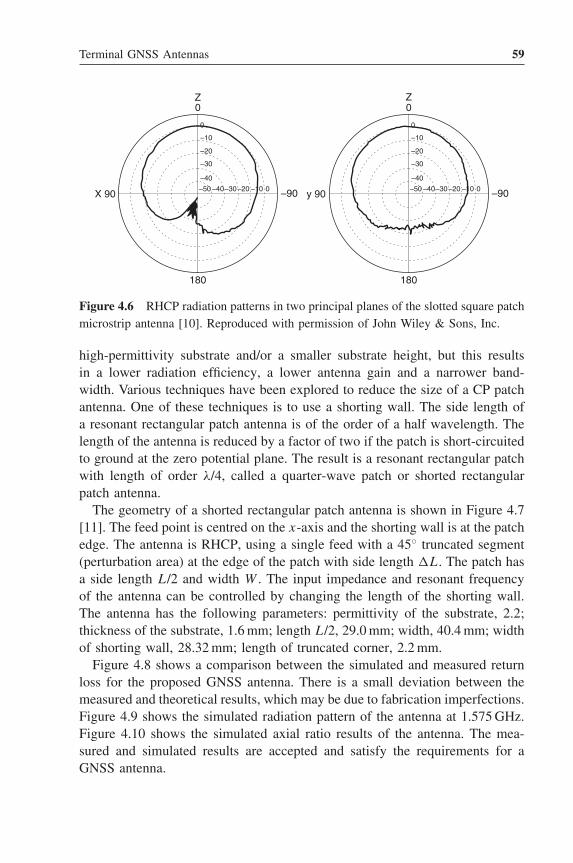
Terminal GNSS Antennas 59
0
0
–10
–20
–30
–40
–50 –40–30–20 –10 0
180
–90X 90
Z0
0
–10
–20
–30
–40
–50 –40–30–20 0
180
–90y 90
Z
–10
Figure 4.6 RHCP radiation patterns in two principal planes of the slotted square patchmicrostrip antenna [10]. Reproduced with permission of John Wiley & Sons, Inc.
high-permittivity substrate and/or a smaller substrate height, but this resultsin a lower radiation efficiency, a lower antenna gain and a narrower band-width. Various techniques have been explored to reduce the size of a CP patchantenna. One of these techniques is to use a shorting wall. The side length ofa resonant rectangular patch antenna is of the order of a half wavelength. Thelength of the antenna is reduced by a factor of two if the patch is short-circuitedto ground at the zero potential plane. The result is a resonant rectangular patchwith length of order λ/4, called a quarter-wave patch or shorted rectangularpatch antenna.
The geometry of a shorted rectangular patch antenna is shown in Figure 4.7[11]. The feed point is centred on the x-axis and the shorting wall is at the patchedge. The antenna is RHCP, using a single feed with a 45◦ truncated segment(perturbation area) at the edge of the patch with side length �L. The patch hasa side length L/2 and width W . The input impedance and resonant frequencyof the antenna can be controlled by changing the length of the shorting wall.The antenna has the following parameters: permittivity of the substrate, 2.2;thickness of the substrate, 1.6 mm; length L/2, 29.0 mm; width, 40.4 mm; widthof shorting wall, 28.32 mm; length of truncated corner, 2.2 mm.
Figure 4.8 shows a comparison between the simulated and measured returnloss for the proposed GNSS antenna. There is a small deviation between themeasured and theoretical results, which may be due to fabrication imperfections.Figure 4.9 shows the simulated radiation pattern of the antenna at 1.575 GHz.Figure 4.10 shows the simulated axial ratio results of the antenna. The mea-sured and simulated results are accepted and satisfy the requirements for aGNSS antenna.

60 Antennas for Global Navigation Satellite Systems
W
L/2
ΔL
Substrate
Shortingwall
Feedpoint
Perturbationarea
Figure 4.7 Geometry of the shorting-wall rectangular microstrip patch antenna [11].Reproduced with permission from JATIT.
0
5
–10
–15
–20
Ret
urn
loss
(d
B)
–25
–30
–351.0 1.5
Frequency (GHz)
2.0
Simulated
Measured
Figure 4.8 Simulated and measured return loss of the shorted rectangular patchantenna [11]. Reproduced with permission from JATIT.
4.1.2 Dual-Feed Microstrip GNSS Antennas
Compared with single-feed structures, dual-feed microstrip GNSS antennashave external polarisers and their structure is more complicated. However,dual-feed microstrip GNSS antennas have high polarisation purity. As shown

Terminal GNSS Antennas 61
0 0–2–4–6–8
–10
–12–12
–10–8–6–4–20
–2–4–6–8
–10–10
–8–6–4–2
0
H-Plane E-Plane
phi = 90 phi = 0330
300
240
210180
150
120
30
60
90270
0
330
300
240
210180
150
120
30
60
90270
0
Figure 4.9 Radiation patterns of the shorting-wall rectangular patch antenna [11].Reproduced with permission from JATIT.
2.0
2.0
1.5
1.5
1.0
0.5
0.0
0.5
1.0
2.0
2.0
1.5
1.5
1.0
0.5
0.0
0.5
1.0
RHCP RHCP
330 30
300
240
210180
150
120
60
90270
0
phi = 0 phi = 90330 30
300
240
210180
150
120
60
90270
0
Figure 4.10 Axial ratio of the shorting-wall rectangular patch [11]. Reproduced withpermission from JATIT.
in Figure 4.11, the proximity-fed microstrip patch antenna supports twoorthogonal modes that combine to deliver RHCP operation. Capacitivelycoupled probe feeds are used to increase impedance matching and bandwidth.Some methods have been presented in the literature to enhance gain at lowangles – for example, employing a folded conducting wall or a dielectriclens and a pyramidal ground, using high-permittivity substrates, or usinga four circular slot–rings array. The design described here employs ahigh-permittivity substrate for encapsulating the patch to increase the gain atlow angles. The permittivity of the substrate is 10.2. The schematic of the90◦ balun which is required to excite the antenna is shown in Figure 4.12. Itcomprises a cascaded 3 dB Wilkinson power divider and a 90◦ phase shifter.It was printed on a microwave substrate with a thickness of 1.5 mm and

62 Antennas for Global Navigation Satellite Systems
lg lpl feed
l feed
lg
lP
X
Y
Z
0°
90°
DhDcap
Figure 4.11 Geometry of the dual-feed, capacitively fed microstrip patch antenna.(Length of the patch, 28 mm; diameter of the capacitive cap, 4 mm; distance betweenthe feed and the centre of the patch, 8 mm; length of the ground, 100 mm, diameter ofthe hole in patch, 3 mm.)
Z1 (lg/4)
Za
Z3 (lg/2)
Z2
Zb
Zb
R
Port 2
Port 3Wilkinson Power Divider 90° Phase Shifter
Port 1
Z1 (lg/4) Z4 (3lg/4)
Figure 4.12 Schematic of the 90◦ balun.
dielectric constant 2.65. For convenience, the characteristic impedances of theinput and output ports of the balun are assumed to be 50 �.
The antenna layer and the feed layer were fixed together. A 50 � SMA con-nector was fitted at the feed point and the Wilkinson divider was terminatedwith a 100 � surface-mounted chip resistor. The final design antenna is shownin Figure 4.13. Figure 4.14 shows the simulated and measured S11, with rea-sonable agreement between the simulated and measured data. The measured
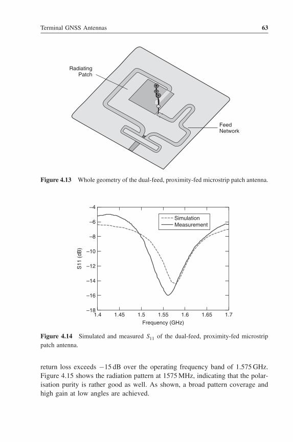
Terminal GNSS Antennas 63
FeedNetwork
RadiatingPatch
Figure 4.13 Whole geometry of the dual-feed, proximity-fed microstrip patch antenna.
1.4 1.45 1.5 1.55 1.6 1.65 1.7–18
–16
–14
–12
–10
–8
–6
–4
Frequency (GHz)
S11
(dB
)
SimulationMeasurement
Figure 4.14 Simulated and measured S11 of the dual-feed, proximity-fed microstrippatch antenna.
return loss exceeds −15 dB over the operating frequency band of 1.575 GHz.Figure 4.15 shows the radiation pattern at 1575 MHz, indicating that the polar-isation purity is rather good as well. As shown, a broad pattern coverage andhigh gain at low angles are achieved.

64 Antennas for Global Navigation Satellite Systems
10.0 –50.0Gain (dB)
10.0
0
0.0
–20.00
–40.00
30RHCP
LHCP
60–60
–30
90
120–120
–90
150–150
–180
Figure 4.15 Radiation pattern of the dual-feed, proximity-fed microstrip patch antennaat 1575 MHz.
4.1.3 Design with Ceramic Substrate
An effective way to achieve a compact GNSS antenna is to use a high-permittivity substrate such as ceramic. Figure 4.16 shows the geometry ofa CP square-disc ceramic chip antenna mounted on a test circuit board forGNSS operation at 1575 MHz [12]. The test circuit board in this study was a0.8 mm grounded FR4 substrate of dimension 50 × 50 mm2. The square-discceramic chip had a height of 4 mm and a cross-section of 17.5 × 17.5 mm2,and its relative permittivity was 45. A square radiating patch of dimension12.6 × 12.6 mm2 was printed and centred on the top surface of the ceramic. Aconducting ground plane is formed on the lower surface of the ceramic. Twoidentical feeds in the form of conformal strips of width 2.2 mm and length 4 mmwere printed at the centres of two adjacent side surfaces of the ceramic chip

Terminal GNSS Antennas 65
Ceramic chip
12.6
Connection metal line50 Ω microstrip line
0.8 mm FR4 substrate
x y
BA
4
Side-feed Side-feed
Ground1
1.5
Ground plane(50 × 50 mm2)
17.5 mm
Figure 4.16 Geometry of square-disc ceramic antenna [12]. Reproduced with permis-sion of John Wiley & Sons, Inc.
and were used to excite the antenna by capacitive coupling. Good impedancematching can be obtained by adjusting the width of the two side-feeds, whichwas chosen to be 2.2 mm.
A connecting metal line 1 mm wide was printed between the two side-feeds.This serves as a delay line to provide a 90◦ phase difference between the twoside-feeds. This phase difference can be obtained by adjusting the distance(1.5 mm in this design) between the connection metal line and the groundconducting patch in the proposed design. Two small notches were cut nearpoints A and B in the ground conducting patch to avoid the short-circuiting ofthe two side-feeds to the ground. To create RHCP radiation, a 50 � microstripfeed line printed on the test circuit board is connected to the side-feed atpoint A; this provides a 90◦ phase lead, relative to the feed at point B. Thisarrangement leads to the excitation of two orthogonal resonant modes of equalamplitude with a 90◦ phase difference for RHCP operation. If LHCP operationis desired for some other applications, the microstrip feed line can be connectedto the side-feed at point B, reversing the relative phases of the feeds.
Figure 4.17 shows the measured return loss of the square-disc ceramicantenna. The impedance bandwidth for a 10 dB return loss is 12 MHz(1570–1582 MHz) centred at 1575 MHz. In addition, there are two resonancesexcited at very close frequencies, which are contributed by the excitation ofthe two side-feeds. Figure 4.18 shows the measured axial ratio in the broadsidedirection of the constructed prototype. With a 3 dB axial ratio a CP bandwidth

66 Antennas for Global Navigation Satellite Systems
1570
0
20
40
Ret
urn
Loss
(dB
)
601555 1565 1575
Frequency (MHz)
1585 1595
1582
Figure 4.17 Measured return loss of the square-disc ceramic antenna [12]. Reproducedwith permission of John Wiley & Sons, Inc.
1572
6
4
2
Axi
al R
atio
(dB
)
01574 1576 1578 1580
Frequency (MHz)
Figure 4.18 Measured axial ratio of the square-disk ceramic antenna [12]. Reproducedwith permission of John Wiley & Sons, Inc.
of about 3.5 MHz is obtained, which covers the required bandwidths for GPSoperation at 1575 MHz. The radiation patterns at 1575 MHz in two principalplanes are also plotted in Figure 4.19, and the gain is shown in Figure 4.20.The measured antenna gain is 3.0–3.4 dBi for operating frequencies acrossthe CP bandwidth with a 3 dB axial ratio.
4.2 Spiral and Helix GNSS Antennas
4.2.1 Helix Antennas
Resonant quadrifilar helical antennas are particularly attractive for GNSS appli-cations because they are small in size and provide circular polarisation and wide

Terminal GNSS Antennas 67
x-z plane
RHCPLHCP
0°
90°–20 –40dB
–90°
y-z plane
0°
90°–20 –40dB
–90°
Figure 4.19 Measured radiation patterns in two principal planes at 1575 MHz [12].Reproduced with permission of John Wiley & Sons, Inc.
1572
4
2
3
1
Ant
enna
Gai
n (d
Bi)
01574 1576 1578 1580
Frequency (MHz)
Figure 4.20 Measured antenna gain of the square-disk ceramic antenna [12]. Repro-duced with permission of John Wiley & Sons, Inc.
elevation coverage. Gerst and Worden studied four-start, six-start and eight-starthelix antennas and showed that the antenna can have different radiation pat-terns and polarisations, and achieve high gain and wide bandwidth [13]. Theresonant fractional-turn quadrifilar helix antenna was introduced by Kilgus [14]in 1968. He described a half-turn, half-wavelength quadrifilar helix as a loop-dipole antenna and showed that circular polarisation is provided, with a widebeamwidth and a cardioid-shaped radiation pattern [15, 16]. The physical struc-ture of the resonant quadrifilar helix proposed in [14] consists of two orthogonalfractional-turn bifilar helical antennas fed in phase quadrature. Each helix pro-duces a toroidal CP pattern. The combination of two orthogonal bifilar helicesprovides a directive CP pattern with the pattern direction determined by thephasing between the two helices. The arrangement consists of two orthogonallybalanced antennas, each of which must be fed through a balun.
An example of a design of a printed half-wavelength quadrifilar helix antennaconsisting of four microstrip-fed helical elements with four opposite radial

68 Antennas for Global Navigation Satellite Systems
Feedregion
Balunshort
Balunshield
To hydrid
Shortcircuit
Radiatingelements
Figure 4.21 Physical configuration of conventional half-turn, half-wavelength quadri-filar helical antenna with Pawsey stub baluns [17]. Reproduced with permissionfrom IET.
strips is shown in Figure 4.21 [17]. This design substitutes microstrip-fedhelical elements for conventional folded or split-sheath baluns. Since the centreconductor of each microstrip-fed helical element is connected to the oppositeradial strip, this connection causes equal currents of opposite phase to flow onthe ground surface of the microstrip feed line and the adjoining radial strip. Theground plane of the microstrip feed line serves as the major radiating elementof the resonant quadrifilar helix antenna.
Figure 4.21 shows the configuration of a conventional half-turn, half-wavelength volute with folded baluns. The upper end of each helical elementis bent to connect to its feed point and the lower end is connected to thebalun shield. At the feed point, opposite helical elements are fed in anti-phaseusing a Pawsey stub balun to form two independent bifilar (balanced) helices.These two bifilar helices are fed in phase quadrature from a 90◦ hybrid toproduce a cardioidal radiation pattern with circular polarisation over the upperhemisphere.
Figure 4.22 shows a printed half-turn, half-wavelength quadrifilar helix fedwith microstrip infinite baluns [17]. The ground plane of each microstrip feedline serves as one of the elements of the bifilar helices. At the feed point, the

Terminal GNSS Antennas 69
Radialstrip
Microstripground
Microstrip
Kaptonlaminate
To hybridHybridground
Figure 4.22 Printed half-turn, half-wavelength quadrifilar helix with infinite microstripbaluns [17]. Reproduced with permission from IET.
centre conductor of the microstrip feed line is soldered to the opposite radialstrip. This causes balanced currents to flow on the outer ground surface ofthe microstrip feed line and the connecting radial strip. This type of balundoes not cause any impedance transformation, so the input impedance of eachmicrostrip-fed helical element can be matched to a 50 � feed line by minoradjustment of the opposite radial strip, without the need for a matching network.
The 90◦ phase relationship between the two pairs of helices can be achievedby exciting the four microstrip-fed helical elements with 0◦, 90◦, 180◦ and270◦ phase differentials. The feed networks can be hybrid types such as thebranch line or rat-race coupler, or T-splitters of either matched or unmatchedform. Feeds using hybrid couplers and matched T-splitters incorporate a fourthport with an absorbing load. These three types of feeding networks give goodisolation between the output ports and will generally provide a wider axial ratiobandwidth than simple splitters. In the prototype design we used a branch-linecoupler to generate the phase quadrature between two bifilar helices.
Figure 4.23 shows the measured return loss for the microstrip-fed printedhalf-turn, half-wavelength quadrifilar helix. The resonant frequency of theantenna is at 1.575 GHz with return loss less than −30 dB. The bandwidthwith l0 dB return loss is 1.6% of the centre frequency.

70 Antennas for Global Navigation Satellite Systems
(iii) Δ
dB
0
–10
–20
–30
–40
Δ (ii)
(i)
1.5754 GHz
Δ
Figure 4.23 Measured return loss of microstrip-fed printed half-turn, half-wavelengthquadrifilar helix antenna [17]. Reproduced with permission from IET.
0
–6
–12
Rel
ativ
e po
wer
, dB
–18
–24
–30180 120 60 0
θ, deg
60 120 180
Figure 4.24 Measured radiation pattern for printed microstrip-fed volute antenna [17].Reproduced with permission from IET.
Figure 4.24 shows the measured radiation pattern of a microstrip-fed printedhalf-turn, half-wavelength quadrifilar helix antenna. As shown in Figure 4.24,a broad axial beam is obtained with a half-power beamwidth of θ > 145◦. Thefront-to-back ratio exceeds 20 dB, which is good for the rejection of multipathsignals reflected from the ground.
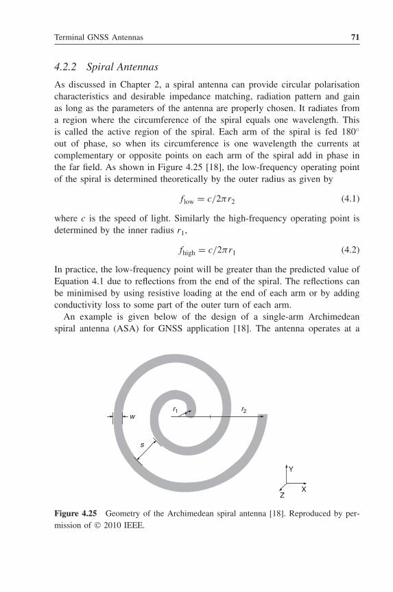
Terminal GNSS Antennas 71
4.2.2 Spiral Antennas
As discussed in Chapter 2, a spiral antenna can provide circular polarisationcharacteristics and desirable impedance matching, radiation pattern and gainas long as the parameters of the antenna are properly chosen. It radiates froma region where the circumference of the spiral equals one wavelength. Thisis called the active region of the spiral. Each arm of the spiral is fed 180◦
out of phase, so when its circumference is one wavelength the currents atcomplementary or opposite points on each arm of the spiral add in phase inthe far field. As shown in Figure 4.25 [18], the low-frequency operating pointof the spiral is determined theoretically by the outer radius as given by
flow = c/2πr2 (4.1)
where c is the speed of light. Similarly the high-frequency operating point isdetermined by the inner radius r1,
fhigh = c/2πr1 (4.2)
In practice, the low-frequency point will be greater than the predicted value ofEquation 4.1 due to reflections from the end of the spiral. The reflections canbe minimised by using resistive loading at the end of each arm or by addingconductivity loss to some part of the outer turn of each arm.
An example is given below of the design of a single-arm Archimedeanspiral antenna (ASA) for GNSS application [18]. The antenna operates at a
r1 r2
s
Y
ZX
w
Figure 4.25 Geometry of the Archimedean spiral antenna [18]. Reproduced by per-mission of © 2010 IEEE.

72 Antennas for Global Navigation Satellite Systems
centre frequency of 1.575 GHz by choosing N = 3r1 = s = w = 0.336 cm, giv-ing r2 = 2.7 cm. The antenna was fed using a coaxial feed and a prototype wasfabricated on FR4 of dielectric constant εr = 4.9 with a thickness of 1.54 mm.Photographs of the fabricated antenna can be seen in Figure 4.26. Figures 4.27and 4.28 show the simulated and measured return loss, respectively, indicating agood resonance at 1.575 GHz. The measured radiation patterns at both x –z andy –z planes are shown in Figure 4.29 and the antenna has an omnidirectionalradiation pattern.
(a) (b)
Figure 4.26 Photographs of the coaxial feed for the Archimedean spiral antenna:(a) top view; (b) bottom view [18]. Reproduced by permission of © 2010 IEEE.
S-Parameter Magnitude in dB0.21497
–5
1.5758Frequency / GHz
–10
–15
–19.886S1,1 : –19.344439
Figure 4.27 Simulated return loss of the Archimedean spiral antenna [18]. Reproducedby permission of © 2010 IEEE.

Terminal GNSS Antennas 73
Ch1 Start Stop 3GHz1GHz Pwr 0dBm
Frequency in GHz
Mea
sure
d S
11 in
dB
S1110
0
–10
–20
–30
–40
–50
–60
–70
M1 1.570000 GHz - 15.881 dB
–M2 1.575000 GHz - 15.443 dB
Tr c1 dB Mag 10 dB/ Ref 0dB Cal
Figure 4.28 Measured return loss of the Archimedean spiral antenna [18]. Reproducedby permission of © 2010 IEEE.
337.5 50
–25–20–15–10
–5
22.5
315
270
202.5
225
247.5
180157.5
(a)
135
112.5
90
45
67.5292.5
337.5 50
–25–20–15–10–5
22.5
315
270
202.5
225
247.5
180157.5
(b)
135
112.5
90
45
67.5292.5
Figure 4.29 Measured radiation patterns of the Archimedean spiral antenna: (a) Eplane; (b) H plane [18]. Reproduced by permission of © 2010 IEEE.
4.3 Design of a PIFA for a GNSS Terminal Antenna
CP antennas have been extensively studied recently for GNSS applications. Thegeneral limitations of the CP patch antennas are the achievable impedance and

74 Antennas for Global Navigation Satellite Systems
axial ratio (AR) bandwidths. Traditionally, the 3 dB AR bandwidth is typicallyless than 10% for the single-feed cases [19, 20]. PIFAs (Planar Inverted-FAntennas) [21–23] have been widely used in wireless communications, as theyhave wideband characteristics, good radiation patterns, simple structures andeasy integration with other active devices, but they are usually used for linearpolarisation. Very few designs are available in the open literature for achievingCP radiation using PIFA structures.
A novel broadband single-feed printed PIFA with broadband circular polar-isation is described in [24], consisting of a square ground with a cross-shapedbranch at its corner and a modified PIFA structure. By introducing a protrud-ing cross at the ground, wideband circular polarisation is generated, and themodified PIFA structure gives the antenna a broad impedance bandwidth. Theantenna has a very compact structure with a dimension of 51 × 13 mm2 on thesubstrate, which is suitable for handheld GNSS terminal application.
The geometry of the proposed broadband planar antenna with broadbandcircular polarisation is shown in Figure 4.30. The antenna uses an FR4 substrate1.6 mm thick with a permittivity of 4.4. The substrate dimension is fixed at94 × 94 mm2. All the metallic components of the antenna are printed on thesame side of the substrate. The antenna consists of a PIFA structure and asquare ground with a cross-shaped branch at its corner. The square ground isplaced in the left part of the substrate with length 68 mm. The antenna is excitedby a coaxial probe. The outer surface of the coaxial is in full conjunction with
L_sub
W_cross
L_cross
L_patch
L_patch
h
L5
L3
WL_feed
Figure 4.30 Geometry of the broadband printed PIFA with circular polarisation.
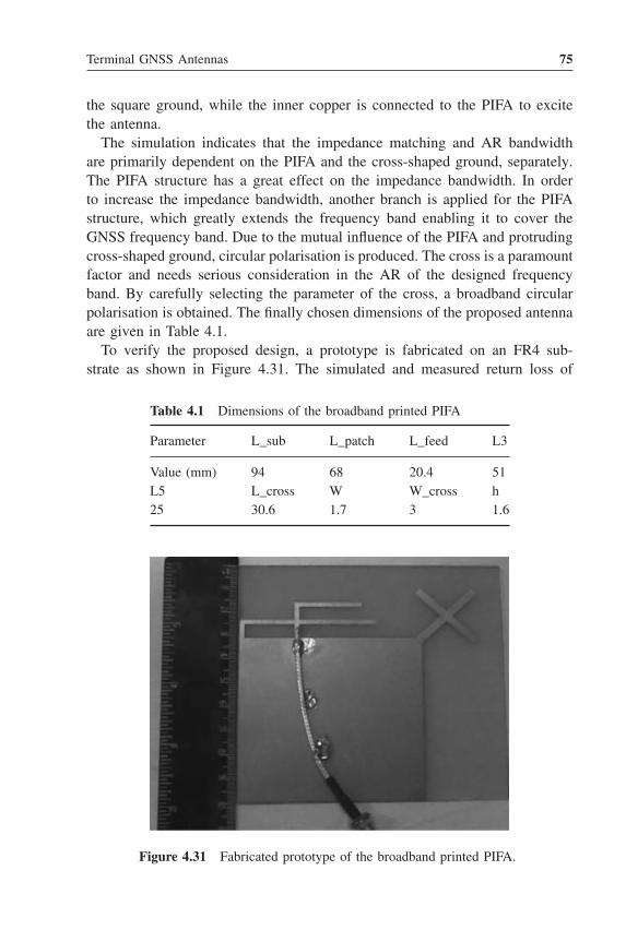
Terminal GNSS Antennas 75
the square ground, while the inner copper is connected to the PIFA to excitethe antenna.
The simulation indicates that the impedance matching and AR bandwidthare primarily dependent on the PIFA and the cross-shaped ground, separately.The PIFA structure has a great effect on the impedance bandwidth. In orderto increase the impedance bandwidth, another branch is applied for the PIFAstructure, which greatly extends the frequency band enabling it to cover theGNSS frequency band. Due to the mutual influence of the PIFA and protrudingcross-shaped ground, circular polarisation is produced. The cross is a paramountfactor and needs serious consideration in the AR of the designed frequencyband. By carefully selecting the parameter of the cross, a broadband circularpolarisation is obtained. The finally chosen dimensions of the proposed antennaare given in Table 4.1.
To verify the proposed design, a prototype is fabricated on an FR4 sub-strate as shown in Figure 4.31. The simulated and measured return loss of
Table 4.1 Dimensions of the broadband printed PIFA
Parameter L_sub L_patch L_feed L3
Value (mm) 94 68 20.4 51L5 L_cross W W_cross h25 30.6 1.7 3 1.6
Figure 4.31 Fabricated prototype of the broadband printed PIFA.

76 Antennas for Global Navigation Satellite Systems
1 1.1 1.2 1.3 1.4 1.5 1.6 1.7 1.8 1.9 2–35
–30
–25
–20
–15
–10
–5
0
Frequency(GHz)
S11
(dB
)
Simulation
Measurement–10dB
Figure 4.32 Simulated and measured return loss for the broadband printed PIFA.
6
5
4
Axi
al R
atio
(dB
)
3
2
1
01 1.1 1.2 1.3 1.4
Frequency(GHz)
1.5 1.6 1.7 1.8
Figure 4.33 Simulated AR of the broadband printed PIFA.

Terminal GNSS Antennas 77
(a) f = 1.17 GHz, x–z plane f = 1.17 GHz, y–z plane
(b) f = 1.23 GHz, x–z plane f = 1.23 GHz, y–z plane
(c) f = 1.57 GHz, x–z plane f = 1.57 GHz, y–z plane
0
–1.00
–7.00
–13.00
–19.00
30
60–60
–30
90
120–120
–90
150–150–180
0
–2.00
–9.00
–15.00
–23.00
30
60–60
–30
90
120–120
–90
150–150–180
0
–2.00
–14.00
–26.00
–38.00
30
60–60
–30
90
120–120
–90
150–150–180
0
–1.00
–7.00
–13.00
–19.00
30
60–60
–30
90
120–120
–90
150–150–180
0
–2.00
–9.00
–16.00
–23.00
30
60–60
–30
90
120–120
–90
150–150–180
0
–2.00
–14.00
–26.00
–38.00
30
60–60
–30
90
120–120
–90
150–150–180
Figure 4.34 The radiation patterns of the broadband printed PIFA at: (a) 1.17 GHz;(b) 1.23 GHz; (c) 1.57 GHz.

78 Antennas for Global Navigation Satellite Systems
2.75
2.50
2.25
2.00
1.75
1.50
1.25dB (
Gai
n T
otal
)
1.00
0.75
0.501.00 1.10 1.20 1.30 1.40
Freq. (GHz)
1.50 1.60 1.70
Ansoft LLC HFSSDesign1XY Plot 8
Figure 4.35 Simulated gain characteristic.
the proposed antenna are shown in Figure 4.32. As can be seen, the S11characteristic shows an improved bandwidth of 46.67% (1.02–1.72 GHz) inmeasurement at less than −10 dB compared with that of 43.33% at less than−10 dB (1.04–1.69 GHz) in simulation.
Figure 4.33 shows the simulated AR in the broadside direction (θ = 0◦).We have just measured AR at a series of discrete points (1176.45, 1207.14,1227.6, 1246, 1268.52, 1278.75, 1561.098, 1575.42, 1605.375 MHz) coveringthe whole GNSS frequency band. As can be seen, the simulation result showsa broadband AR bandwidth of around 660 MHz from 1.07 to 1.73 GHz for AR≤3 dB, which is largely enhanced compared with a microstrip antenna.
The radiation patterns in the x –z and y –z planes at three different frequen-cies (L1, L2, L5 for GPS) are given in Figure 4.34. The solid curve representsthe RHCP pattern, while the dashed line represents the LHCP pattern. As canbe seen, the antenna achieves good CP radiation in the z-direction.
The simulated gain characteristics of the antenna are shown in Figure 4.35.We find that in all GNSS frequency bands the gain of the antenna is above1.5 dBi, which is well above the requirement for handheld wireless terminals.
This chapter has introduced practical microstrip patches, quadrifilar helicesand spirals for application with GNSS receivers. Most of these antenna designs

Terminal GNSS Antennas 79
can only operate in a single frequency band. Antenna designs for operating inmultiple GNSS frequency bands and for other special scenarios are discussedin the next chapter.
References1. Lu, J.H., Tang, C.L. and Wong, K.L., ‘Single feed slotted equilateral-triangular microstrip
antenna for circular polarization’, IEEE Transactions on Antennas and Propagation , 47,1174–1178, 1999.
2. Yang, K.P., Wong, K.L. and Lu, J.H., ‘Compact circularly-polarized equilateral-triangularmicrostrip antenna with Y-shaped slot’, Microwave and Optical Technology Letters , 20,31–34, 1999.
3. Chen, W.S., Wu, C.K. and Wong, K.L., ‘Novel compact circularly polarized square microstripantenna’, IEEE Transactions on Antennas and Propagation , 49, 340–342, 2001.
4. Bokhari, S.A., Zuercher, J.F., Mosig, J.R. and Gardiol, F.E., ‘A small microstrip patchantenna with a convenient tuning option’, IEEE Transactions on Antennas and Propagation ,44, 1521–1528, 1996.
5. Tang, C.L. and Wong, K.L., ‘A modified equilateral-triangular-ring microstrip antenna forcircular polarization’, Microwave and Optical Technology Letters , 23, 123–126, 1999.
6. Chen, W.S., Wu, C.K. and Wong, K.L., ‘Compact circularly polarized microstrip antennawith bent slots’, Electronic Letters , 34, 1278–1279, 1998.
7. Chen, W.S., Wu, C.K. and Wong, K.L., ‘Compact circularly polarized circular microstripantenna with cross slot and peripheral cuts’, Electronic Letters , 34, 1040–1041, 1998.
8. Lu, J.H. and Wong, K.L., ‘Single-feed circularly-polarized equilateral-triangular microstripantenna with a tuning stub’, IEEE Transactions on Antennas and Propagation , 48, 1869–1872,2000.
9. Wong, K.L. and Chen, M.H., ‘Slot-coupled small circularly polarized microstrip antenna withmodified cross-slot and bent tuning-stub’, Electronic Letters , 34, 1542–1543, 1998.
10. Sim, C.Y.D. and Han, T.Y., ‘GPS antenna design with slotted ground plane’, Microwave andOptical Technology Letters , 50 (3), 818–821, 2008.
11. Abdelaziz, A.A. and Nashaat, D.M., ‘Compact GPS microstrip patch antenna’, Journal ofTheoretical and Applied Information Technology , 4, 530–535, 2007.
12. Su, C.M. and Wong, K.L., ‘Surface-mountable dual side-feed circularly polarized ceramicchip antenna’, Microwave and Optical Technology Letters , 35 (2), 137–138, 2002.
13. Gerst, C. and Worden, R., ‘A helix antenna takes turn for better’, Electronics , 39 (17),100–110, 1966.
14. Kilgus, C.C., ‘Multi-element, fractional turn helices’, IEEE Transactions on Antennas andPropagation , 16, 400–500, 1968.
15. Kilgus, C.C., ‘Resonant quadrifilar helix’, IEEE Transactions on Antennas and Propagation ,17, 349–451, 1969.
16. Kilgus, C.C., ‘Resonant quadrifilar helix design’, Microwave Journal , 13, 49–54, 1970.17. Shumaker, P.K., Ho, C.H. and Smith, K.B., ‘Printed half-wavelength quadrifilar helix antenna
for GPS marine applications’, Electronics Letters , 32 (3), 153–154, 1996.

80 Antennas for Global Navigation Satellite Systems
18. Mohd Yusop, M.F., Ismail, K., Sulaiman, S. and Haron, M.A., ‘Coaxial feed Archimedeanspiral antenna for GPS application’, Proceedings of the 2010 IEEE Asia-Pacific Conferenceon Applied Electromagnetics (APACE 2010).
19. Iwasaki, H., ‘A circularly polarized small-size microstrip antenna with a cross slot’, IEEETransactions on Antennas and Propagation , 44 (10), 1399–1401, 1996.
20. Wang, C.L. and Chang, K., ‘A novel CP patch antenna with a simple feed structure’, Antennaand Propagation Society International Symposium, Vol. 2, pp. 1000–1003, 2000.
21. Rowell, C.R. and Murch, R.D., ‘A compact PIFA suitable for dual-frequency 900/1800-MHzoperation’, IEEE Transactions on Antennas and Propagation , 46, 596–598, 1998.
22. Wong, K.L. and Huang, C.H., ‘Bandwidth-enhanced PIFA with a coupling feed for quad-bandoperation in the mobile phone’, Microwave and Optical Technology Letters , 50, 683–687,2008.
23. Kuo, Y.L., Chiou, T.W. and Wong, K.L., ‘A novel dual-band printed inverted-F antenna’,Microwave and Optical Technology Letters , 31, 353–355, 2001.
24. Wang, X., Yao, Y., Lu, Z.J., Yu, J.S. and Chen, X., ‘A broadband planar antenna withcircular polarization for multi-mode satellite navigation’, Asia-Pacific Microwave Conference,Melbourne, Australia, 5–8 December 2011.

5Multimode and AdvancedTerminal Antennas
This chapter introduces multimode antennas for an integrated GNSS receiver,covering the GPS, GLONASS, Compass and Galileo systems. It presentsseveral kinds of multimode GNSS antennas, including microstrip and helixantennas. For each one, some practical and novel designs are presented, such asmulti-layer microstrip antennas, slotted-patch antennas, quadrifilar helix anten-nas, and so on. Finally, the chapter touches on high-precision terminal antennasfor differential GPS, including phase centre determination and stability.
5.1 Multiband Terminal Antennas
With the development of satellite navigation technology, many countrieshave started to build their own satellite navigation systems. Nowadays, thesesystems are used intensively. The American GPS and the Russian GLONASSare already operating worldwide. The Chinese Compass system has alsoprovided a partial service. Future satellite navigation receivers will providemultimode operation utilising different satellite navigation systems to improvetheir positioning accuracy and reliability, so the design of terminal antennasfor multimode satellite navigation systems is practically desirable.
A multimode satellite navigation receiver is required to cover several fre-quency bands for the GPS, GLONASS, Galileo and Compass systems, asdetailed in Table 1.1. Each GNSS has several frequency bands. The challengesin the design of a multiband receiver antenna come from two requirements: theantenna needs to provide right hand circular polarisation with a low axial ratio
Antennas for Global Navigation Satellite Systems, First Edition.Xiaodong Chen, Clive G. Parini, Brian Collins, Yuan Yao and Masood Ur Rehman.© 2012 John Wiley & Sons, Ltd. Published 2012 by John Wiley & Sons, Ltd.

82 Antennas for Global Navigation Satellite Systems
and also maintain a low VSWR over multiple frequency bands. In this chapterseveral designs of dual-band and triple-band GNSS antennas are discussed.
5.1.1 Multiband Microstrip GNSS Antennas
Because of their low profile, CP microstrip antennas are widely used in GNSSapplications. However, most of the current antenna designs only cover theGPS L1 band: 1575 MHz. In more demanding operations, such as differentialGPS [1], it is necessary that terminal antennas cover multiple GNSS bands.There are generally two kinds of microstrip antennas capable of multibandRHCP operation. One uses stacked patches while the other uses a single patchwith loading.
5.1.1.1 Design of a Stacked Patch with a Single Feed
A CP antenna for multi-frequency operation can be achieved by usingmulti-layer patches. By using a multi-layer structure it is easier to achievemulti-frequency CP operation than can be provided using other approaches.The dimensions of each patch mainly determine the resonant frequencies. Bychanging one of the patches, a specific frequency can be achieved while therest of the frequencies remain unchanged [2].
Based on the principle mentioned above, we propose a multi-layer microstrippatch antenna operating at three frequencies with circular polarisation. Thegeometry of the proposed antenna is shown in Figure 5.1. The triple-layerpatch antenna is fed by a single coaxial cable that passes through the groundplane and substrates and is connected to the top patch. The top, middle andbottom layer patches of the antenna are for the 575, 1227 and 1176 MHz bandsrespectively. RHCP is achieved by placing the feed point in the upper rightportion of the diagonal of the square patch.
In Figure 5.1, each square patch is built on a substrate of permittivityεr = 2.65 and the same substrate height of h = 1.5 mm. The size of groundplane is 100 mm. The dimensions of each patch (ai × bi) and feed position(c, d) need to be optimised in order to minimise the VSWR and AR. Thedetailed size is: a1 = b1 = 55.5 mm, a2 = b2 = 71 mm, a3 = b3 = 74 mm andc = d = 8 mm. Figure 5.2 shows the simulation results for return loss. Theresonant frequencies are 1575, 1227 and 1176 MHz, matching the target fre-quencies well. The bandwidths of VSWR < 2 at each frequency are 35, 16 and25 MHz for each band. Figure 5.3 shows the AR of the antenna. The antennaradiates RHCP at all three frequencies; the radiation patterns are presentedin Figure 5.4.

Multimode and Advanced Terminal Antennas 83
a1
a2
a3
Ground
Feed Point
h1h2
h3
b3 b2 b1
Figure 5.1 Structure of three-layer microstrip CP antenna.
1 1.1 1.2 1.3 1.4 1.5 1.6–25
–20
–15
–10
–5
0
Frequency (GHz)
S11
(dB
)
Figure 5.2 Return loss of the three-layer microstrip CP antenna.

84 Antennas for Global Navigation Satellite Systems
1 1.1 1.2 1.3 1.4 1.5 1.60
10
5
15
20
25
30
Frequency (GHz)
AR
(dB
)
Figure 5.3 Axial ratio of the three-layer microstrip CP antenna.
5.0 –20.0 5.0
Freq = 1.175 GHzFreq = 1.225 GHz
Freq = 1.575 GHz
0
30
dB(GainRHCP) [db]
60–60
–305.00
–5.00
0.0
–10.00
–15.00
90
120–120
–90
150–150
–180
Figure 5.4 RHCP radiation patterns of the three-layer microstrip CP antenna.

Multimode and Advanced Terminal Antennas 85
5.1.1.2 Design of Stacked Patches with Four Feeds [3]
This antenna design comprises two stacked patches which are fed by four pinsplaced symmetrically on the two main axes. The amplitude and phase relation-ship between the four pins to maintain circular polarisation is obtained by twowideband 90◦ hybrid couplers. Impedance matching of the four-feed structureis easily realised by changing the positions of the feed points. The structure ofthe antenna is shown in Figure 5.5. The antenna consists of two square patcheswith tuning stubs, stacked concentrically in the vertical direction. Changing thelength of the tuning stubs can alter the resonance frequency, which will declinewhen the lengths of the tuning stubs increase. The permittivity of both the toptwo substrates is 9.8 (εr1 = εr2 = 9.8), and their thicknesses are both 2.5 mm(h1 = h2 = 2.5 mm). The feed network layer uses a square substrate of FR4. Itsthickness is 0.8 mm (h3 = 0.8 mm) and length 48 mm. All the structures havea via with a diameter of 1.5 mm (D = 1.5 mm) at their centre, so that the twopatches on the top and bottom layers can be connected to the ground. Thus theradiation patterns are directed towards the z-axis. The feed network is composedof two 3 dB wideband 90◦ hybrids whose ground is common to the ground ofthe antenna – it is shown as one ground in the figure. The dimensions of the two
1
d
(–b, 0)
T1
W1
y
L1
(0, a)4
3 x
(a, 0)
2
(0, –b)
(b)
y
x
(0, a)
(a, 0)1
4
32
(–b, 0)
(0, –b)
T2
L2
D
W2
(c)
(a)
Top patch
Bottom patch
GroundFeed network layer
S2
S1
h1h2
h3
r2εr1 1 2 3 4ε
Figure 5.5 Geometry of the four-feed stacked antenna: (a) side view; (b) top patch;(c) bottom patch [3]. Reproduced by permission of © 2007 IEEE.

86 Antennas for Global Navigation Satellite Systems
0
–5
–10
–15
S11
(dB
)
–20
S11
(dB
)
0
–5
–10
–15
–20
–25
1.00
E+009
(a) (b)1.
20E+00
9
1.40
E+009
1.60
E+009
1.80
E+009
2.00
E+009
2.00
E+009
2.20
E+009
2.40
E+009
2.60
E+009
2.80
E+009
3.00
E+009
(Hz) (Hz)
Figure 5.6 Measured S11 of the four-feed stacked antenna [3]. Reproduced by per-mission of © 2007 IEEE.
patches are L1 = 17.5 mm and L2 = 26 mm, and the dimensions of the tuningstubs are T1 = 1.5 mm, W1 = 2.5 mm, T2 = 1 mm, W2 = 5 mm. The two sub-strates have dimensions S1 = 63 mm and S2 = 73 mm; the lengths from pin tocentre are a = 3 mm and b = 5 mm. Pin 1 and pin 2, used for feed points of thelower frequency band, are connected to the bottom patch but do not touch thetop patch. The diameter of the pin is 1 mm (d = 1 mm). Pin 3 and pin 4 are usedfor feed points of the higher frequency band; they too are connected to the toppatch but do not touch the bottom patch. The currents fed to pin 1 and pin 2, andthat fed also to pin 3 and pin 4, must maintain equal amplitude and 90◦ phasedifference so that the antenna receives RHCP signals at both frequency bands.
As shown in Figure 5.6, the antenna resonates in both the L band (1.6 GHz)and S band (2.5 GHz). Figure 5.7 shows that the measured AR of the antennais less than 6 dB when the elevation is in the range of 0◦ –60◦ at lower fre-quency, and is less than 3.5 dB when the elevation is in the range of 0◦ –90◦
at higher frequency. The measured and simulated results have the same trend,but there are some differences between them. This is due to the errors of theamplitude and phase of the actual feed network. Figure 5.8 shows the linearradiation patterns of the antenna. The 3 dB beamwidth at the lower frequencyis larger than 140◦ and at higher frequency is larger than 160◦. It has perfectCP characteristics over a wide angle.
5.1.1.3 Design of Single Patch with Loading
A new design of a single-layer slit-loaded square patch antenna for achievingdual-band circular polarisation has been reported [4]. The antenna size can be

Multimode and Advanced Terminal Antennas 87
Elevation (degrees) Elevation (degrees)
(a) (b)
9
7
8
6
5
4
3Axi
al R
atio
(dB
)
2
1
–90–80–70–60–50–40–30–20–10 0 10 20 30 40 50 60 70 80 90
0
Measured value
Simulated value
5.0
4.0
4.5
3.5
3.0
2.5
2.0
Axi
al R
atio
(dB
)
1.5
1.0
0.5
–90–80–70–60–50–40–30–20–10 0 10 20 30 40 50 60 70 80 90
0.0
Measured value
Simulated value
Figure 5.7 AR results of the antenna at (a) lower frequency and (b) higher frequency[3]. Reproduced by permission of © 2007 IEEE.
–30
–30
–35
–35
–40
–40
–45
–45
–50
–50
–30
–30
–35
–35
–40
–40
–45
–45
–50
–50
–55
–55
–60
30
60
120
150180
150
120
30
60
9090
030
60
120
150180
150
120
30
60
9090
0
(a) (b)
Figure 5.8 Radiation patterns of the antenna at (a) lower frequency and (b) higherfrequency [3]. Reproduced by permission of © 2007 IEEE.
significantly reduced compared with conventional stacked-patch CP designs.The proposed slit-loaded square patch antennas are formed by inserting fourT-shaped slits at the patch edges or four Y-shaped slits at the patch cornersof a square patch as shown in Figure 5.9. The two resonant modes TM01 andTM03 are excited to provide dual-band CP radiation in the designs. Due tothe inserted T-shaped or Y-shaped slits, the surface current path of the TM01mode is greatly lengthened, which effectively lowers its resonant frequencyand allows the designs to operate with a reduced patch size for a fixed lowerfrequency. The inserted slits also considerably lower the resonant frequency ofthe TM03 mode and modify its three-lobe-shaped radiation pattern to become
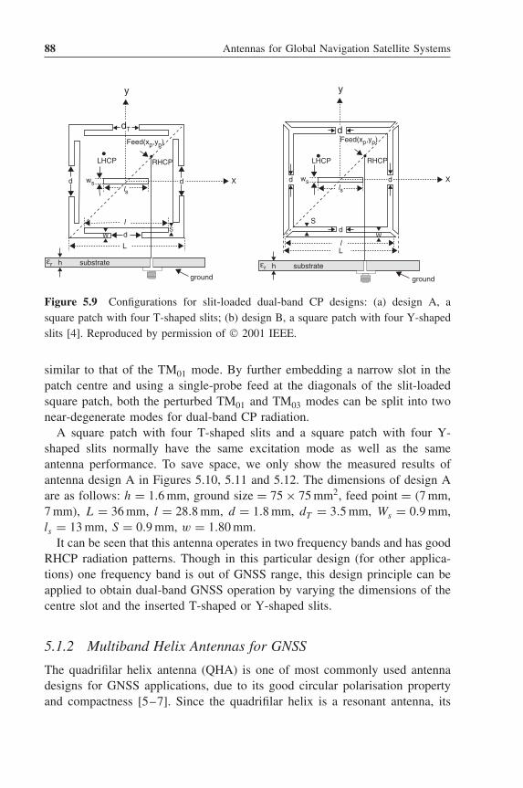
88 Antennas for Global Navigation Satellite Systems
y
LHCP RHCP
ground
X
S
d
d
d
L
ls
l
ws
εr h substrate
W
dT
Feed(xp,yp)
y
RHCP
L
d
lW
S
LHCP
Xls
ws
ground
εr h substrate
Feed(xp,yp)
dd
d
Figure 5.9 Configurations for slit-loaded dual-band CP designs: (a) design A, asquare patch with four T-shaped slits; (b) design B, a square patch with four Y-shapedslits [4]. Reproduced by permission of © 2001 IEEE.
similar to that of the TM01 mode. By further embedding a narrow slot in thepatch centre and using a single-probe feed at the diagonals of the slit-loadedsquare patch, both the perturbed TM01 and TM03 modes can be split into twonear-degenerate modes for dual-band CP radiation.
A square patch with four T-shaped slits and a square patch with four Y-shaped slits normally have the same excitation mode as well as the sameantenna performance. To save space, we only show the measured results ofantenna design A in Figures 5.10, 5.11 and 5.12. The dimensions of design Aare as follows: h = 1.6 mm, ground size = 75 × 75 mm2, feed point = (7 mm,7 mm), L = 36 mm, l = 28.8 mm, d = 1.8 mm, dT = 3.5 mm, Ws = 0.9 mm,ls = 13 mm, S = 0.9 mm, w = 1.80 mm.
It can be seen that this antenna operates in two frequency bands and has goodRHCP radiation patterns. Though in this particular design (for other applica-tions) one frequency band is out of GNSS range, this design principle can beapplied to obtain dual-band GNSS operation by varying the dimensions of thecentre slot and the inserted T-shaped or Y-shaped slits.
5.1.2 Multiband Helix Antennas for GNSS
The quadrifilar helix antenna (QHA) is one of most commonly used antennadesigns for GNSS applications, due to its good circular polarisation propertyand compactness [5–7]. Since the quadrifilar helix is a resonant antenna, its

Multimode and Advanced Terminal Antennas 89
1513
0
10
20
30
40
501000 1500 2000
Frequency (MHz)
2500 3000 3500
Ret
urn
Loss
(dB
)
1566
1538 MHz3050 MHz
2987 3085
Figure 5.10 Measured return loss for design A: a square patch with four T-shapedslits [4]. Reproduced by permission of © 2001 IEEE.
0
1
2
3
4
Axi
al R
atio
(dB
)
1538 MHz
1528 1546
1525 1535 1545
3050 MHz
3034 3066
3030 3050 3070
Figure 5.11 Measured AR for design A: a square patch with four T-shaped slits [4].Reproduced by permission of © 2001 IEEE.
dimensions are chosen to provide optimal performance for one frequency band,and it is difficult to design it to operate at multiple frequency bands. Variousmethods have been proposed to make the QHA operate at both GPS frequen-cies of 1.575 and 1.227 GHz. A typical approach is to use volutes of differentsize and construction [8]. Another technique is to place a parallel LC circuitat appropriate locations in each arm [9]. The antenna provides the same per-formance in two separate frequency bands and has no impact upon the overallsize by this method.
The configuration of a compact printed square QHA antenna for dual-bandGNSS application is shown in Figure 5.13 [10]. The antenna is mounted abovea substrate and has the shape of a cube, formed by four vertical substrate

90 Antennas for Global Navigation Satellite Systems
(a)
(b)RHCPLHCP
0°
90°x-z plane
−90°
0°
90°y-z plane
−90°
0°
90°–10 –30dB x-z plane
−90°
0°
90°y-z plane
−90°
Figure 5.12 Measured radiation patterns for design A: a square patch with fourT-shaped slits [4]. Reproduced by permission of © 2001 IEEE.
Ground plane
FR4
Rogers 5880
Connected to the ground (G)
Connected tothe feeder
network (A)
Figure 5.13 Geometry of the dual-band QHA [10]. Reproduced with permission ofJohn Wiley & Sons, Inc.
boards, each of which has a printed helix on one face. These printed helicescomprise two loops having different lengths. The total length of the shorter loopis chosen to be about one-quarter of a wavelength at 1575 MHz, and that of thelonger loop is about one-quarter of a wavelength at 1227 MHz. The antennacan radiate RHCP, and the sense of polarisation is determined by the directionof rotation of the printed helices. The feed network is required to produce fourRF signals of equal amplitude with relative phases of 0◦, 90◦, 180◦ and 270◦.The antenna, combined with the feed network, generates CP radiation. Thevolume of the antenna is 1 cm3.

Multimode and Advanced Terminal Antennas 91
D
A B
C.
. .
.
Figure 5.14 Layout of the feed network of the dual-band QHA [10]. Reproduced withpermission of John Wiley & Sons, Inc.
–5
–10
–15
–20
| S11
|, d
B
–25
–30
–351 1.1 1.2 1.3 1.4 1.5
Frequency, GHz
1.6 1.7 1.8 1.9 2
Figure 5.15 Measured S11 of the dual-band QHA [10]. Reproduced with permissionof John Wiley & Sons, Inc.
The feed network is designed by using microstrip lines printed on the FR4substrate, which has a permittivity of 4.6 and thickness of 1.6 mm. Figure 5.14shows the layout of the feed network, which uses three Wilkinson powerdividers and different lengths of connecting microstrip lines to achieve therequired relative phases. As the feed network needs to operate at both 1227and 1575 MHz, it is designed at a centre frequency of 1400 MHz.
The measured S11, as shown in Figure 5.15, is below −10 dB at both 1227and 1575 MHz bands. Figures 5.16 shows the measured radiation patterns at1227 and 1575 MHz. It can be seen that the cross-polar level is 10 dB below
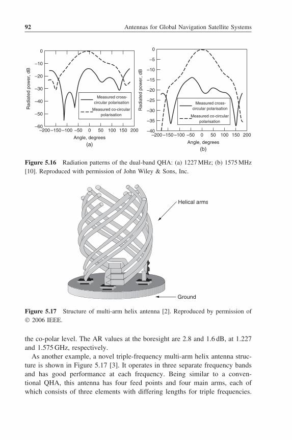
92 Antennas for Global Navigation Satellite Systems
0 0
–10–10
–15
–20
–25
–30
–35
–40
–5
–20
–30
–40
Rad
iate
d po
wer
, dB
Rad
iate
d po
wer
, dB
–50
–60–200–150–100 –50
Angle, degrees
(a)
0 50 100 150 200–200 –150 –100 –50
Angle, degrees
(b)
0 50 100 150 200
Measured cross-circular polarisation
Measured co-circularpolarisation
Measured cross-circular polarisation
Measured co-circularpolarisation
Figure 5.16 Radiation patterns of the dual-band QHA: (a) 1227 MHz; (b) 1575 MHz[10]. Reproduced with permission of John Wiley & Sons, Inc.
Helical arms
Ground
Figure 5.17 Structure of multi-arm helix antenna [2]. Reproduced by permission of© 2006 IEEE.
the co-polar level. The AR values at the boresight are 2.8 and 1.6 dB, at 1.227and 1.575 GHz, respectively.
As another example, a novel triple-frequency multi-arm helix antenna struc-ture is shown in Figure 5.17 [3]. It operates in three separate frequency bandsand has good performance at each frequency. Being similar to a conven-tional QHA, this antenna has four feed points and four main arms, each ofwhich consists of three elements with differing lengths for triple frequencies.
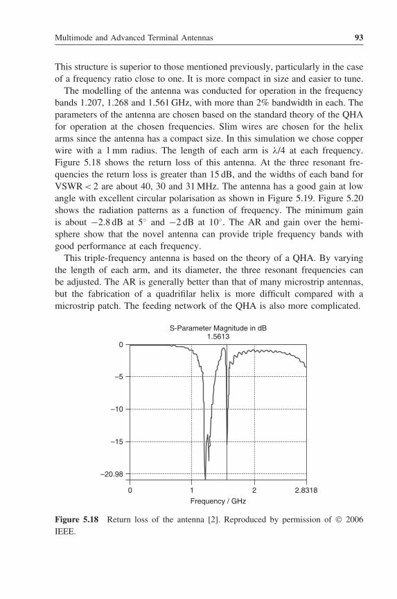
Multimode and Advanced Terminal Antennas 93
This structure is superior to those mentioned previously, particularly in the caseof a frequency ratio close to one. It is more compact in size and easier to tune.
The modelling of the antenna was conducted for operation in the frequencybands 1.207, 1.268 and 1.561 GHz, with more than 2% bandwidth in each. Theparameters of the antenna are chosen based on the standard theory of the QHAfor operation at the chosen frequencies. Slim wires are chosen for the helixarms since the antenna has a compact size. In this simulation we chose copperwire with a 1 mm radius. The length of each arm is λ/4 at each frequency.Figure 5.18 shows the return loss of this antenna. At the three resonant fre-quencies the return loss is greater than 15 dB, and the widths of each band forVSWR < 2 are about 40, 30 and 31 MHz. The antenna has a good gain at lowangle with excellent circular polarisation as shown in Figure 5.19. Figure 5.20shows the radiation patterns as a function of frequency. The minimum gainis about −2.8 dB at 5◦ and −2 dB at 10◦. The AR and gain over the hemi-sphere show that the novel antenna can provide triple frequency bands withgood performance at each frequency.
This triple-frequency antenna is based on the theory of a QHA. By varyingthe length of each arm, and its diameter, the three resonant frequencies canbe adjusted. The AR is generally better than that of many microstrip antennas,but the fabrication of a quadrifilar helix is more difficult compared with amicrostrip patch. The feeding network of the QHA is also more complicated.
0
–5
–10
–15
0 1 2
Frequency / GHz
S-Parameter Magnitude in dB1.5613
2.8318
–20.98
Figure 5.18 Return loss of the antenna [2]. Reproduced by permission of © 2006IEEE.

94 Antennas for Global Navigation Satellite Systems
120
150
210
240270
300
330
60
–30 –20 –10
30
0180
90
0 [dB]
1.207 GHz1.268 GHz1.551 GHz
Figure 5.19 AR of the antenna [2]. Reproduced by permission of © 2006 IEEE.
1.207 GHz1.268 GHz1.561 GHz
1.207 GHz1.268 GHz1.561 GHz
(a) f = 0° (b) f = 90°
120
150
210
240
270
300
330
60
–20 –10 0
30
0180
90
120
150
210
240
270
300
330
60
–20 –10 0
30
0180
90
10 [dB] 10 [dB]
Figure 5.20 Radiation patterns of the antenna [2]. Reproduced by permission of© 2006 IEEE.

Multimode and Advanced Terminal Antennas 95
5.2 Wideband CP Terminal Antennas
As described previously, the whole frequency band of the four GNSSs (GPS,GLONASS, Compass, Galileo) is between 1164 and 1615.5 MHz and thisrequires an antenna with a relative impedance bandwidth of 33%. Another wayto achieve multimode GNSS operation is to develop a wideband CP antenna tocover this 33% relative impedance bandwidth. In this section, several antennasare discussed to show a broadband GNSS performance.
5.2.1 Wideband Microstrip Antenna Array
A four-element wideband CP array, which utilises multi-layer microstrip patchantenna technology, was successfully designed and tested [11]. Each unit of thearray comprised four dielectric substrates that incorporate electromagneticallycoupled radiating elements fed by microstrip feed lines through coupling slots.The substrate architecture for the four-layer microstrip antenna design is shownin Figure 5.21, where adjacent substrates (Rogers 4003, h = 1.524 mm) are setd = 10 mm apart vertically. Three elements located on three separate layers,together with a slot-coupled feed, provide the required bandwidth. Each elementhas vertical (VP) and horizontal (HP) feed points.
This single-element design was arranged in a 2 × 2 array with a centre-to-centre separation of 65 mm. The architecture and prototype are illustrated inFigure 5.22. As shown in Figure 5.23, the array has good impedance matchingand an excellent boresight AR performance of less than 1.5 dB over the entire
h
HP
d VP Feednetwork
Ground/slot
Patch 1
Patch 2
Patch 3
Figure 5.21 Architecture of a four-layer array unit. Taken from [11]; copyrightEurAAP; used with permission.

96 Antennas for Global Navigation Satellite Systems
Zm
Figure 5.22 Prototype of four-element microstrip antenna array. Taken from [11];copyright EurAAP; used with permission.
four GNSS system band. The gain of the antenna is above 8.5 dBi for thedesignated operating band.
5.2.2 High-Performance Universal GNSS Antenna Basedon Spiral Mode Microstrip Antenna Technology
A class of high-performance low-cost GNSS antennas that covers all threeGNSS services (GPS/GLONASS/Galileo) is described in [12]. This low-costantenna is platform conformable. The prototype is shown in Figure 5.24, whichis a spiral mode microstrip (SMM) antenna 11.5 cm in diameter and 3.0 cm inheight. The antenna is a four-arm self-complementary Archimedean spiral. Itscharacteristics are shown in Figure 5.25, illustrating a broad bandwidth. Its lowprofile and conformable shape make it suitable for platform mounting.
5.2.3 Wideband CP Hybrid Dielectric Resonator Antenna
Circular polarisation can also be generated by using a dielectric resonatorantenna (DRA) with two orthogonal feeds. A recent approach to improve thebandwidth of DRAs consists of merging the resonant band of the dielectricresonator with a band produced by the feed network itself. Such an antenna isreferred to as a hybrid dielectric resonator antenna [13].
A hybrid antenna comprising a DRA and four feed slots as shown inFigure 5.26 has been investigated and analysed to enhance the AR bandwidthin order to cover the current GNSS frequency bands in one antenna [14].
The cylindrical DRA has a radius of 31.75 mm, a height of 22 mm and apermittivity of 10. It has been designed to resonate around 1.575 GHz. Circu-lar polarisation is generated by a 90◦ phase feed network. The slots have tobe arranged and their dimensions optimised to ensure proper coupling to the

Multimode and Advanced Terminal Antennas 97
MARKER 11.175 GHz–16.136 dB
MARKER 21.225 GHz–19.301 dB
MARKER 31.38 GHz–15.961 dB
MARKER 5 1.575 GHzpoint 116
MARKER 41.38 GHz–15.961 dBMARKER 51.575 GHz–13.399 dB
START1.0 GHz
S11
S
C
1.1 GHz
1
1 23
51.6 GHz
REF 0.0 dB log MAG10.0 dB/
–13.339 dB
STOP2.0 GHz
28 OCT 0813:28:20
1175 MHz3
2.5
2
1.5
Axi
al R
atio
(dB
)
1
0.5
01100 1200 1300 1400 1500
Frequency (MHz)
1600
1575 MHz
Figure 5.23 Measured S11 and AR performance of four-element microstrip antennaarray. Taken from [11]; copyright EurAAP; used with permission.
dielectric resonator and to have good impedance matching. A substrate made ofFR4 was chosen to accommodate the feed circuit of the DRA and the slots wereetched in the ground plane. The ground plane dimensions are 160 × 160 mm2;the slot length is 36 mm and its width is 8.8 mm. The coordinates of the slots

98 Antennas for Global Navigation Satellite Systems
(a) (b)
Spiral element
Z
X
q
Feed network and ground planeSide-mounted
RF connectorOptional bottom-mountedRF connector
Figure 5.24 (a) Cross-sectional view for layout and (b) photograph of universal GNSSantenna [12]. Reproduced by permission of © 2010 IEEE.
SWR
2
1
1.000 GHz 2.000
(a) (b)
REF = 1.000 U 1.000 U/DIV z
y
5 dB/division
Figure 5.25 Universal GNSS antenna characteristics: (a) SWR performance;(b) measured radiation pattern (RHCP) [12]. Reproduced by permission of © 2010IEEE.
are 4 mm along the x-direction and 19.4 mm in the y-direction. The feed lineis 12.9 mm long and 11 mm away from the slot centre. The prototype of theDRA and its performance are shown in Figures 5.27 and 5.28. The advantageof the hybrid DRA over other GNSS antennas is its compact size.
5.2.4 Multi-Feed Microstrip Patch Antenna for Multimode GNSS
Note that a general limitation on CP microstrip antennas is the achievableAR bandwidth while the impedance bandwidth is satisfied. Traditionally, the

Multimode and Advanced Terminal Antennas 99
Y
X
Microstripline
SlotSsx
Smx
Ssy
Ws
Wgnd
Lm
LS
Z
X
Feeding lines Substrate
DRA
h
Groundplane
Figure 5.26 Diagram of the hybrid DRA [14]. Reproduced by permission of © 2010IEEE.
allowable 3 dB AR bandwidth is typically less than 10% for the single-feedcases [15, 16]. Much wider impedance and AR bandwidths can be achieved indual-feed and quadruple-feed CP patch antennas. Experimental patch anten-nas with quadruple broadband feeds [16, 17] have been found to achieve−10 dB impedance bandwidths of around 70–80% and 3 dB AR bandwidthsof 80%.
Figure 5.29 shows an example of a four-feed microstrip antenna for a wide-band GNSS application [17]. Four small, square radiating patches situated underthe parasitic patch are excited by four metallic probes mounted symmetricallyin the +z-direction. In order to enlarge the AR bandwidth, a symmetrical con-figuration of the antenna elements is necessary. The feed network model for
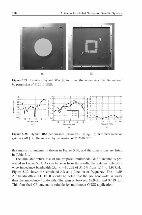
100 Antennas for Global Navigation Satellite Systems
(a) (b)
Figure 5.27 Fabricated hybrid DRA: (a) top view; (b) bottom view [14]. Reproducedby permission of © 2010 IEEE.
Axi
al R
atio
at B
ores
ight
[dB
]
54.5
3.54
32.5
21.5
10.5
01.2 1.3 1.4 1.5 1.6
Frequency [GHz]
(c)
Ret
urn
Loss
[dB
]
0
–5
–10
–15
–20
–25
–30
–35
–401 1.2 1.4 1.6 1.8
Frequency [GHz]
(a)
2
54.5
4
3.53
2.5
Max
imum
Rea
lised
[dB
]
2
1.51
0.50
1.2 1.3 1.4 1.5 1.6
Frequency [GHz]
(b)
f = 0°f = 45°f = 90°
Figure 5.28 Hybrid DRA performance (measured): (a) S11; (b) maximum radiationgain; (c) AR [14]. Reproduced by permission of © 2010 IEEE.
this microstrip antenna is shown in Figure 5.30, and the dimensions are listedin Table 5.1.
The simulated return loss of the proposed multimode GNSS antenna is pre-sented in Figure 5.31. As can be seen from the results, the antenna exhibits awide impedance bandwidth (S11 < −10 dB) of 51.6% from 1.14 to 1.93 GHz.Figure 5.32 shows the simulated AR as a function of frequency. The −3 dBAR bandwidth is 1 GHz. It should be noted that the AR bandwidth is widerthan the impedance bandwidth. The gain is between 6.69 dBi and 8.429 dBi.This four-feed CP antenna is suitable for multimode GNSS application.
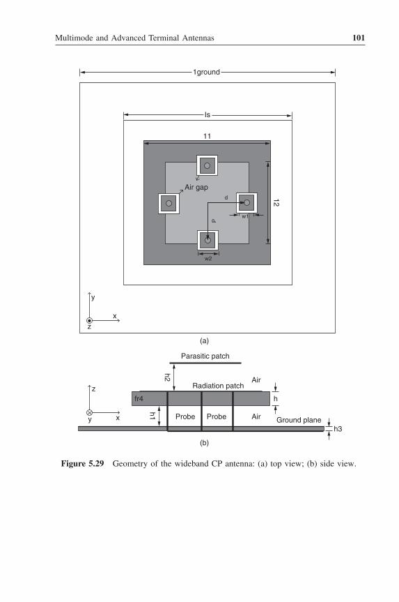
Multimode and Advanced Terminal Antennas 101
1ground
Is
11
Parasitic patch
Radiation patch
Probe Probe
h3
Air
Air
(a)
(b)
z
x
fr4
y
zx
y
Ground plane
h
12
h2
h1
Air gapd
w1
w2
P
Figure 5.29 Geometry of the wideband CP antenna: (a) top view; (b) side view.

102 Antennas for Global Navigation Satellite Systems
2C2C
C C
L
L
2C2CL
L
Wilkinson power divider
Quadrature power splitter
180° broadband phase shifter
0° Port 1
90°Port 2
180°Port 3
270° Port 4
CRLH CRLH
Port 0
Figure 5.30 Broadband five-port phase shifter and feed network providing currentsof equal amplitude and phase of 0◦, 90◦, 180◦ and 270◦.
Table 5.1 Dimensions of the antenna (units: mm)
d h h1 h2 l1 l2 ls lground w1 w2
25.6 3 12 10 64.8 55 84 100 6 9
5.3 High-Precision GNSS Terminal Antennas
High-precision satellite positioning has been widely used in applications includ-ing marine and terrestrial geodesy, geodynamics, astronomy, geophysical explo-ration, resource exploration, engineering survey deformation monitoring andcivil engineering. To provide enhanced accuracy of location, receivers for theseapplications make use of the information contained in the phase of the incomingsatellite, so maintaining the stability of the phase centre of the antenna is veryimportant in the antenna design.
What the satellite navigation system measures is the distance between thephase centres of the transmitting receiving antennas. The satellite navigation

Multimode and Advanced Terminal Antennas 103
1 1.1 1.2 1.3 1.4 1.5 1.6 1.7 1.8 1.9 2
–5
–10
–15
–20
–25
0
Frequency (GHz)
S11
(dB
)
Figure 5.31 Simulated return loss of the wideband CP antenna.
1 1.1 1.2 1.3 1.4 1.5 1.6 1.7 1.8 1.9 2
0.2
0.15
0.1
0.05
0
0.25
Frequency (GHz)
AR
(dB
)
Figure 5.32 Simulated AR of the wideband CP antenna.
receiver needs to track signals from several satellites simultaneously; each satel-lite has different elevation and azimuth angles as seen from the receiver, sovariations in the antenna phase centre when seen from different elevation andazimuth angles will give rise to position errors. The phase centre of the antennais the benchmark of the observations of the satellite navigation receiver, whilethe placement of the antenna is based on the geometric centre. Any distancebetween these two centres will cause some measurement error. Movement of the

104 Antennas for Global Navigation Satellite Systems
phase centre as a function of elevation angle mainly causes altitude errors. Phasecentre changes associated with the azimuth will result in errors in positioningin the horizontal plane. According to the stability of the phase centre of theantenna, these errors vary from a millimetre to a few centimetres. For pseudo-code ranging, this error is much smaller than the positioning accuracy, so it canbe ignored, but for a carrier phase measurement used for high-precision posi-tioning, this error cannot be ignored. A detailed discussion on the antenna phasecentre and evaluation of the phase centre variation is presented in Appendix B.
A typical method of achieving stability of the antenna phase centre is tomaintain the symmetry of the antenna structure. In the design of microstrippatch antennas, an axisymmetric multiple feed is often used to obtain antennaphase centre stability, since the antenna structure is itself symmetrical. In gen-eral, the more feed points and the better the physical symmetry of the antenna,the higher the stability of the phase centre, but at the cost of more complexityof the feed network. Also, microstrip patch antennas with axisymmetric mul-tiple feeds suffer from narrow bandwidth. A multi-arm spiral antenna ensuresthe high-stability properties of the phase centre through spiral arms which aresymmetrical around the axis.
As an example, we present here a multi-feed dual-band GPS patch antennadeveloped by Trimble Zephyr [18]. This antenna utilises an innovative n-pointsymmetrical feed patch design, where n is a positive integer greater than two,as shown in Figure 5.33. There is a significant improvement in terms of phasecentre stability compared with a single-feed design. The key feature of thismulti-feed design is its perfect symmetry in structure, obtained through com-bining a phased multiple feed system and precisely located feed points.
L1 Element
L2 Element
N Feed Points
Phase Centre Error Ellipsoid, close totrue centre and very small
Figure 5.33 The Trimble Zephyr antenna with symmetrical n-point feed [18]. Source:www.Trimble.com.
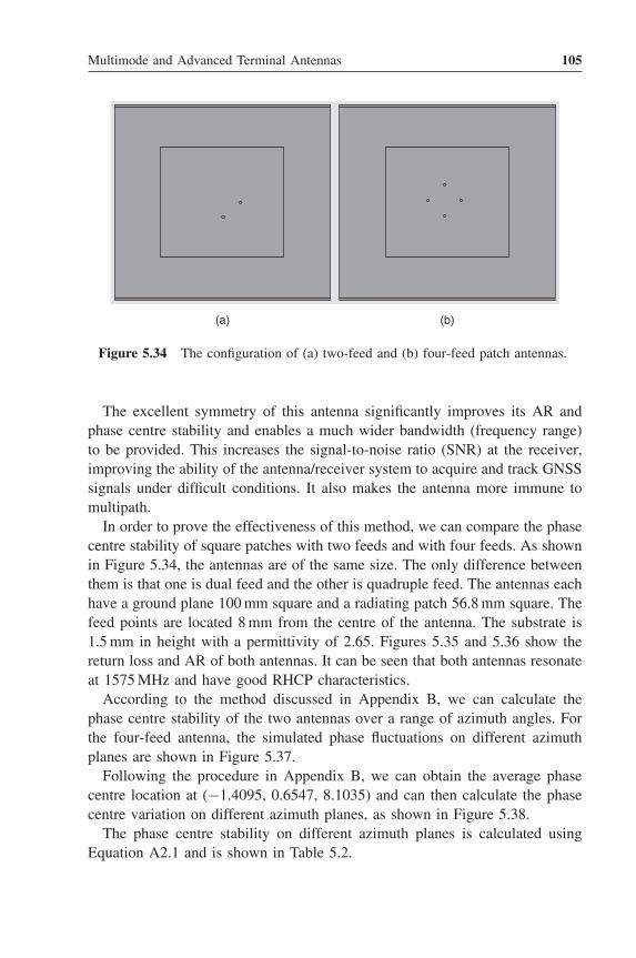
Multimode and Advanced Terminal Antennas 105
(a) (b)
Figure 5.34 The configuration of (a) two-feed and (b) four-feed patch antennas.
The excellent symmetry of this antenna significantly improves its AR andphase centre stability and enables a much wider bandwidth (frequency range)to be provided. This increases the signal-to-noise ratio (SNR) at the receiver,improving the ability of the antenna/receiver system to acquire and track GNSSsignals under difficult conditions. It also makes the antenna more immune tomultipath.
In order to prove the effectiveness of this method, we can compare the phasecentre stability of square patches with two feeds and with four feeds. As shownin Figure 5.34, the antennas are of the same size. The only difference betweenthem is that one is dual feed and the other is quadruple feed. The antennas eachhave a ground plane 100 mm square and a radiating patch 56.8 mm square. Thefeed points are located 8 mm from the centre of the antenna. The substrate is1.5 mm in height with a permittivity of 2.65. Figures 5.35 and 5.36 show thereturn loss and AR of both antennas. It can be seen that both antennas resonateat 1575 MHz and have good RHCP characteristics.
According to the method discussed in Appendix B, we can calculate thephase centre stability of the two antennas over a range of azimuth angles. Forthe four-feed antenna, the simulated phase fluctuations on different azimuthplanes are shown in Figure 5.37.
Following the procedure in Appendix B, we can obtain the average phasecentre location at (−1.4095, 0.6547, 8.1035) and can then calculate the phasecentre variation on different azimuth planes, as shown in Figure 5.38.
The phase centre stability on different azimuth planes is calculated usingEquation A2.1 and is shown in Table 5.2.

106 Antennas for Global Navigation Satellite Systems
1.5 1.52 1.54 1.56 1.58 1.6–35
–30
–25
–20
–15
–10
–5
0
Frequency (GHz)
S11
(dB
)
1.5 1.52 1.54 1.56 1.58 1.6–10
–8
–6
–4
–2
0
Frequency (GHz)
S11
(dB
)(a) (b)
Figure 5.35 Return loss of (a) two-feed and (b) four-feed patch antennas.
1.5 1.52 1.54 1.56 1.58 1.60.1
0.12
0.14
0.16
0.18
0.2
0.22
Frequency (GHz)
(a) (b)
AR
(dB
)
0.2
0.15
0.1
0.05
0
0.25
1.5 1.52 1.54 1.56 1.58 1.6Frequency (GHz)
AR
(dB
)
Figure 5.36 The AR of (a) two-feed and (b) four-feed patch antennas.
For the dual-feed patch antenna, the simulated phase fluctuations for differentazimuth planes are shown in Figure 5.39.
Following the same procedure in Appendix B, we can obtain the phase cen-tre location (1.1153,–0.8344, 6.9164) and can then calculate the phase centrevariation, as shown in Figure 5.40.
So the phase centre stability on different azimuth planes is calculated usingEquation A2.1 again, and is shown in Table 5.3. It can be seen that the antennawith four feeds has a more stable phase centre than the one with dual feeds.
We have discussed a variety of multiband and wideband GNSS antennasin this chapter and have addressed the issue of phase centre stability in high-precision GNSS terminal antennas. However, we have not considered the effects

Multimode and Advanced Terminal Antennas 107
–60 –40 –20 0 20 40 60–200
–150
–100
–50
0
50
100
150
200
Theta (degrees)
rER
HC
P (
degr
ees)
Phi = 0°Phi = 60°Phi = 120°Phi = 180°
Figure 5.37 The phase pattern of RHCP remote electric field (rERHCP) on differentazimuth planes for θ = ±60◦ of four-feed antenna.
1.5
1
0.5
0
–0.5
–1
–1.5
Ph
ase
Pat
tern
(de
gree
s)
–2
–2.5
–3
–3.5–60 –40 –20
Theta (degrees)
0 20 40 60
0
60
120
180
Figure 5.38 Phase centre variation of rERHCP on different azimuth planes for θ =±60◦ of four-feed antenna.
Table 5.2 Phase centre stability with respect to azimuthal angles for four-feed patchantenna
Azimuth angle � 0◦ 30◦ 60◦ 90◦ 120◦ 150◦ 180◦
Phase centre stability (mm) 1.0753 0.9212 0.5112 0.7678 0.6905 1.007 1.0753

108 Antennas for Global Navigation Satellite Systems
–60 –40 –20 0 20 40 60–200
–150
–100
–50
0
50
100
150
200
Theta (degrees)
rER
HC
P (
degr
ees)
Phi = 0°Phi = 60°Phi = 120°Phi = 180°
Figure 5.39 The phase pattern of rERHCP at different azimuth planes for θ = ±60◦
of dual-feed antenna.
Pha
se P
atte
rn (
degr
ee)
–5
–4
–3
–2
–1
0
1
2
–60 –40 –20
Theta (degrees)
0 20 40 60
0
60
120
180
Figure 5.40 Phase centre variation of rERHCP on different azimuth planes forθ = ±60◦ of dual-feed antenna.
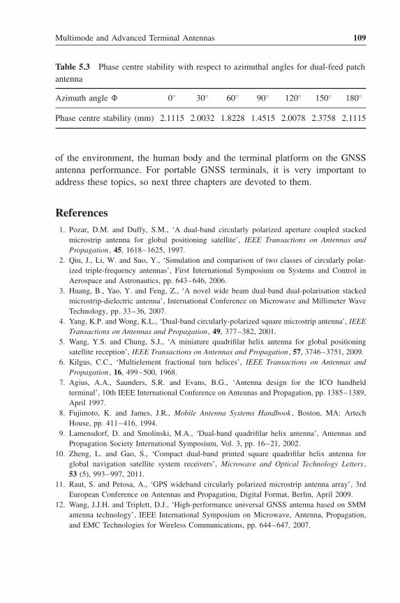
Multimode and Advanced Terminal Antennas 109
Table 5.3 Phase centre stability with respect to azimuthal angles for dual-feed patchantenna
Azimuth angle � 0◦ 30◦ 60◦ 90◦ 120◦ 150◦ 180◦
Phase centre stability (mm) 2.1115 2.0032 1.8228 1.4515 2.0078 2.3758 2.1115
of the environment, the human body and the terminal platform on the GNSSantenna performance. For portable GNSS terminals, it is very important toaddress these topics, so next three chapters are devoted to them.
References1. Pozar, D.M. and Duffy, S.M., ‘A dual-band circularly polarized aperture coupled stacked
microstrip antenna for global positioning satellite’, IEEE Transactions on Antennas andPropagation , 45, 1618–1625, 1997.
2. Qiu, J., Li, W. and Suo, Y., ‘Simulation and comparison of two classes of circularly polar-ized triple-frequency antennas’, First International Symposium on Systems and Control inAerospace and Astronautics, pp. 643–646, 2006.
3. Huang, B., Yao, Y. and Feng, Z., ‘A novel wide beam dual-band dual-polarisation stackedmicrostrip-dielectric antenna’, International Conference on Microwave and Millimeter WaveTechnology, pp. 33–36, 2007.
4. Yang, K.P. and Wong, K.L., ‘Dual-band circularly-polarized square microstrip antenna’, IEEETransactions on Antennas and Propagation , 49, 377–382, 2001.
5. Wang, Y.S. and Chung, S.J., ‘A miniature quadrifilar helix antenna for global positioningsatellite reception’, IEEE Transactions on Antennas and Propagation , 57, 3746–3751, 2009.
6. Kilgus, C.C., ‘Multielement fractional turn helices’, IEEE Transactions on Antennas andPropagation , 16, 499–500, 1968.
7. Agius, A.A., Saunders, S.R. and Evans, B.G., ‘Antenna design for the ICO handheldterminal’, 10th IEEE International Conference on Antennas and Propagation, pp. 1385–1389,April 1997.
8. Fujimoto, K. and James, J.R., Mobile Antenna Systems Handbook , Boston, MA: ArtechHouse, pp. 411–416, 1994.
9. Lamensdorf, D. and Smolinski, M.A., ‘Dual-band quadrifilar helix antenna’, Antennas andPropagation Society International Symposium, Vol. 3, pp. 16–21, 2002.
10. Zheng, L. and Gao, S., ‘Compact dual-band printed square quadrifilar helix antenna forglobal navigation satellite system receivers’, Microwave and Optical Technology Letters ,53 (5), 993–997, 2011.
11. Raut, S. and Petosa, A., ‘GPS wideband circularly polarized microstrip antenna array’, 3rdEuropean Conference on Antennas and Propagation, Digital Format, Berlin, April 2009.
12. Wang, J.J.H. and Triplett, D.J., ‘High-performance universal GNSS antenna based on SMMantenna technology’, IEEE International Symposium on Microwave, Antenna, Propagation,and EMC Technologies for Wireless Communications, pp. 644–647, 2007.

110 Antennas for Global Navigation Satellite Systems
13. Clenet, M., Caillet, M. and Antar, Y.M.M., ‘Wideband circularly polarized antenna elementsfor GPS/GNSS applications developed at DRDC Ottawa’, 14th International Symposium onAntenna Technology and Applied Electromagnetics (ANTEM) and the American Electro-magnetics Conference (AMEREM), pp. 1–4, 2010.
14. Massie, G., Caillet, M., Clenet, M. and Antar, Y.M.M., ‘A new wideband circularly polarizedhybrid dielectric resonator antenna’, IEEE Antennas and Wireless Propagation Letters , 9,347–350, 2010.
15. Iwasaki, H., ‘A circularly polarized small-size microstrip antenna with a cross slot’, IEEETransactions on Antennas and Propagation , 44, 1399–1401, 1996.
16. Wang, C. and Chang, K., ‘A novel CP patch antenna with a simple feed structure’, Antennasand Propagation Society International Symposium, Vol. 2, pp. 1000–1003, 2000.
17. Tao, J., Yu, J. and Chen, X., ‘A design of multi-mode global navigation satellite systemantenna’, Chinese Scientific Papers Online, 18 January 2011.
18. Krantz, E., Riley, S. and Large, P., ‘GPS antenna design and performance advance-ments: The Trimble Zephyr’, http://trl.trimble.com/docushare/dsweb/Get/Document-86094/5700WPZephyrE.pdf (accessed 4 November 2011).

6Terminal Antennas in DifficultEnvironments
6.1 GNSS Antennas and Multipath Environment
The introduction of built-in GPS in portable personal navigation devices(PNDs), especially in mobile phones, has revolutionised the navigationindustry. The ever-growing demand for the availability of navigation facilitiesin these devices has made the GNSS an essential part of modern wirelesspersonal area network (WPAN) and wireless body area network (WBAN)applications. As the only navigation and positioning service provider to themobile phone industry in recent times, the GPS is discussed in this chapter.
Portable mobile terminals are affected by multipath due to reflections, diffrac-tion and scattering of the incident radio waves. It depends on the structure ofthe surrounding environment, as shown in Figure 6.1. This phenomenon hasbeen well studied over time. Analysis of this complex and random nature prob-lem is complicated. Statistical modelling is a powerful tool that offers simpleand flexible solutions to such problems. A number of researchers have usedthis approach to study and characterise the multipath effects on mobile termi-nals and GPS antennas [1–10]. Axelrad et al. have used signal-to-noise ratios(SNRs) to predict and remove multipath errors [7]. Wu and Hsieh have usedsidereal filtering of time-series range residual variations based on a least squaresmodel to mitigate the multipath [8]. It requires a comprehensive data set con-taining multipath delay samples from the previous day and the day beforethat. Spangenberg et al. have modelled the multipath as the variance changein received signals in line-of-sight (LOS) conditions and as mean value jumps
Antennas for Global Navigation Satellite Systems, First Edition.Xiaodong Chen, Clive G. Parini, Brian Collins, Yuan Yao and Masood Ur Rehman.© 2012 John Wiley & Sons, Ltd. Published 2012 by John Wiley & Sons, Ltd.

112 Antennas for Global Navigation Satellite Systems
BlockedReflection
Reflection
Diffraction
BlockedDiffraction
MultipathEnvironment
AUT
PreceivedGPS
MultipleDiffraction
BlockedPath Direct
Path
PincidentGPS = P⊥ + P||
P⊥
P||
Figure 6.1 GPS environment and multipath signals. Reproduced by permission of© 2012 IEEE.
in non-line-of-sight (NLOS) conditions using an extended Kalman filter [9].Hannah has proposed a parabolic-equation-based propagation model for GPSmultipath employing the concept of coupled polarisation reflection coefficient[10]. However, these studies usually need large measurement data sets andmainly deal with quantification of multipath effects on stand-alone, static GPSreceivers with antennas designed according to the theoretical guidelines.
Ideally, the GPS antennas should have good RHCP with a uniform radiationpattern over the entire upper hemisphere to receive the incoming GPS sig-nal efficiently. A good rejection of LHCP is also required to avoid multipath[11–13]. However, these requirements are difficult to fulfil in portable devices,especially in mobile terminals that are required to allow maximum mobility ofthe user and flexibility of use with multiple functions such as Wi-Fi, Bluetooth,FM radio, digital camera, mobile TV and GPS [14, 15].

Terminal Antennas in Difficult Environments 113
In the common scenarios of cluttered environments including indoors andcity streets, LOS GPS signals arriving at the mobile terminal are weak whilethe reflected signals may have arbitrary polarisations. Moreover, mobile phonesare hardly used in a fixed position and the ‘up’ direction of the antenna changesdepending on the used orientation. Furthermore, the antenna suffers from elec-tromagnetic absorptions and shielding of clear sky view in hand held positions.Establishing a quick GPS link with good satellite lock is therefore a difficult taskin such devices. Use of wide-beam linear polarised (LP) GPS antennas couldhelp to address the uncertainty of antenna orientation, blockage of LOS signaland clear sky view, and losses due to the user’s body. Hence, LP antennasare a preferred choice for mobile terminal GPS as they give better perfor-mance compared with the conventional RHCP antennas [16–18]. Moreover, itenables use of the multipath signal constructively in order to establish a quickGPS link. Once a GPS lock is achieved, positioning errors can be estimatedand removed using software approaches. This necessitates the characterisationof mobile terminal GPS antennas in a multipath environment.
Mean effective gain (MEG) has been used as an important performancemetric for mobile handsets in multipath land mobile propagation environments[19, 20]. It describes statistically the impact of the antenna on the link budgetconsidering the angle of arrival and polarisation of the incident waves andantenna gain characteristics [1–4]. Effects of the presence of the human bodycan also be evaluated using this technique [5, 6]. The applicability of this metricto portable GPS antennas in conjunction with another new parameter of antennacoverage efficiency has been proposed and developed by Ur Rehman et al.[21–23]. This chapter investigates the usefulness of this method, presenting athorough analysis of mobile terminal GPS antennas.
6.2 Statistical Modelling of Multipath Environment for GNSSOperation
Currently, the performance assessment of a mobile terminal GPS antenna ismostly done by field tests. However, it has the drawback of longer procedureswhere weather, temperature and location hazards make it hard to control the testenvironment. It results in lack of accuracy due to poor repeatability and effi-ciency. The statistical models representing the real multipath scenarios providean excellent alternative to the field tests, predicting the antenna performancewhile avoiding the shortcomings of the field tests.
A statistical method is developed to characterise the environmental factorson the performance of the GPS antennas, introducing the parameters of GPS

114 Antennas for Global Navigation Satellite Systems
mean effective gain (MEGGPS) and coverage efficiency (ηc). The MEG equationderived by Taga [1] is reformulated to suit the GPS environment with RHCPincoming waves and environmental reflections. An overview of the expectedperformance of the GPS antennas in the multipath environment can be achievedusing this method by knowing the 3D free space antenna gain patterns and theaverage angular distribution of incident power in the environment.
6.2.1 GPS Mean Effective Gain (MEGGPS)
The MEG is the average gain of the antenna performance in a multipath radioenvironment. The MEG of an antenna in a mobile terminal is defined as [1]
MEG = mean received power (Preceived)
total mean incident power (Pincident)(6.1)
For spherical coordinates (Figure 6.2), Preceived can be expressed as [24]
Preceived =∫ 2π
0
∫ π
0
[P1Gθ (θ, φ) pθ (θ, φ)
+P2Gφ (θ, φ) pφ (θ, φ)]
sin θ dθ dφ (6.2)
where Gθ (θ, φ) and Gφ (θ, φ) are θ and φ components of the antenna powergain pattern respectively and pθ (θ, φ) and pφ (θ, φ) indicate the θ and φ
components of angular density functions of the incoming waves, respectively.P1 is the mean power that would be received by an isotropic antenna in θ
polarisation while P2 is the mean power received by an isotropic antenna in φ
polarisation. The total mean incident power (Pincident) arriving at the antenna isthe summation of the mean powers in the two polarisations.
The incident wave in the GPS mobile environment can be split into twocomponents, namely the perpendicular polarised component and the parallelpolarised component. Therefore, θ and φ components respectively correspondto the perpendicular and parallel polarised components. Reformulating Equation6.2 to suit the GPS environment results in the following:
PreceivedGPS=
∫ 2π
0
∫ π
0
[P⊥G⊥ (θ, φ) p⊥ (θ, φ)
+P||G|| (θ, φ) p|| (θ, φ)]
sin θ dθ dφ (6.3)
Now, P⊥ and P|| are the mean received powers in the perpendicular and parallelpolarisations with respect to the ground plane while p⊥ (θ, φ) and p|| (θ, φ)
represent the perpendicular and parallel components of the angular density

Terminal Antennas in Difficult Environments 115
Incident wave distributionin elevation plane
Incident wave distributionin azimuth plane
Antennaunder test
Z
q
f
X
Y
Figure 6.2 Spherical coordinates system and representation of a hypothetical incidentwave distribution model. Reproduced by permission of © 2012 IEEE.
functions of the incoming waves respectively, as shown in Figure 6.1. Pincidentarriving at the mobile GPS terminal is then
PincidentGPS= P⊥ + P|| (6.4)
The ratio between the mean powers received in the two polarisations is calledthe Cross-Polarisation Ratio (XPR) and described as
XPR = P⊥P||
(6.5)
Using Equations 6.3–6.5, the MEG expression for the GPS antenna can beformulated as [22, 23]
MEGGPS =∫ 2π
0
∫ π
0
[XPR
1 + XPRG⊥(θ, φ)p⊥(θ, φ)
+ 1
1 + XPRG‖(θ, φ)p||(θ, φ)
]sin θ dθdφ (6.6)

116 Antennas for Global Navigation Satellite Systems
Ground Ground
Random RHCP hemisphericalincident waves from GPS satellite
IncidentWave
ReflectedWave
qi qrAUT
AUT
Reflected Electric waves(Angle Dependent)
Figure 6.3 Multipath environment model around the mobile terminal GPS receiverantenna [22]. Reproduced with permission from IET.
Since XPR governs the polarisation of the incoming wave in this model,the circular polarised (CP) nature of the incoming GPS satellite signal isaccumulated by making XPR = 0 dB. It employs the fact that simultaneoustransmission of two LP waves that have a phase difference of π/2 (radians)results in the generation of a CP wave.
6.2.2 GPS Angle of Arrival Distribution (AoAGPS)
The AoAGPS gives a statistical definition of the direction of arrival of theincident radio waves, arriving at the mobile terminal GPS antenna. Boththe azimuth and elevation planes should be considered separately to replicatethe multipath environment.
The incident radio waves are reflected, diffracted and scattered from theobjects located in the surroundings of the receiving antenna. Since these objectsvary in height and shape, the direction of arrival of the incident waves israndom. This random occurrence is dealt with by a uniform angular densityfunction in azimuth, similar to the case of the land mobile environment [1–3].For the GPS environment, reflections from the ground (Figure 6.3) should alsobe considered in the elevation plane. The elevation plane is therefore dividedinto incident and reflection regions. Due to the lack of available measurementdata for the direction of arrival of the GPS waves, the angular density functionis assumed to be uniform in the incident region. In the reflection region, it is nolonger uniform and reduced by a factor governed by the reflection coefficients.Also, the favourable use of the multipath signal in the mobile terminal GPSantennas for quick link establishment leads to use the summation of the receivedpowers in the incident and reflected regions.
In accordance with the preceding assumptions, the statistical model for theGPS antenna in an open field multipath environment with ground reflections is

Terminal Antennas in Difficult Environments 117
proposed as follows [22, 23, 25]:
p⊥(θ, φ) ={
1 0 ≤ θ ≤ π/2A(θ)⊥ π/2 ≤ θ ≤ π
(6.7)
p‖(θ, φ) ={
1 0 ≤ θ ≤ π/2A(θ)‖ π/2 ≤ θ ≤ π
(6.8)
A (θ) depends upon the reflection coefficients for the perpendicular and par-allel components that vary with angle of incidence (θi) as [26]
A(θi)⊥ =cos θi −
√(ε2/ε1) − sin2 θi
cos θi +√
(ε2/ε1) − sin2 θi
(6.9)
A(θi)|| =(ε2/ε1) cos θi −
√(ε2/ε1) − sin2 θi
(ε2/ε1) cos θi +√
(ε2/ε1) − sin2 θi
(6.10)
In this study, the open field ground is considered to be of a semi-grassy, semi-concrete type with a relative permittivity of 4.5 [27, 28]. It makes the modela replication of the open field working environment. Having the knowledge ofAoAGPS, the model could be easily adapted to an urban environment.
6.2.3 GPS Coverage Efficiency (ηc)
Coverage efficiency of the receiving GPS antenna is another important parame-ter. It defines the capability of the antenna to receive the signals coming directlyfrom the satellites.
The GPS antenna can receive signals from all directions that lie within itscoverage area. However, the performance of a GPS antenna is currently charac-terised by its ability to receive the signals for elevation angles higher and lowerthan 10◦ (from the horizon) [12]. Defining the antenna coverage based on thiscriterion fails to describe its overall coverage in the upper hemisphere. The con-cept of coverage efficiency overcomes this drawback by providing informationabout the antenna coverage in the whole upper hemisphere.
The coverage efficiency of the antenna under test is calculated as the ratioof the solid angles subtended by its coverage area to the total area [22, 23]:
ηc = coverage area
total area(6.11)
These calculations are based on the RHCP gain pattern of the antenna undertest to suit the RHCP incoming radio waves. The coverage area depends on
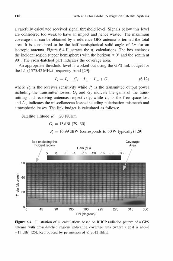
118 Antennas for Global Navigation Satellite Systems
a carefully calculated received signal threshold level. Signals below this levelare considered too weak to have an impact and hence wasted. The maximumcoverage that can be obtained by a reference GPS antenna is termed the totalarea. It is considered to be the half-hemispherical solid angle of 2π for anisotropic antenna. Figure 6.4 illustrates the ηc calculations. The box enclosesthe incident region (upper hemisphere) with the horizon at 0◦ and the zenith at90◦. The cross-hatched part indicates the coverage area.
An appropriate threshold level is worked out using the GPS link budget forthe L1 (1575.42 MHz) frequency band [29]:
Pr = Pt + Gt − Lp − Lm + Gr (6.12)
where Pr is the receiver sensitivity while Pt is the transmitted output powerincluding the transmitter losses. Gt and Gr indicate the gains of the trans-mitting and receiving antennas respectively, while Lp is the free space lossand Lm indicates the miscellaneous losses including polarisation mismatch andatmospheric losses. The link budget is calculated as follows:
Satellite altitude R = 20 180 km
Gt = 13 dBi [29, 30]
Pt = 16.99 dBW (corresponds to 50 W typically) [29]
Box enclosing theincident region
CoverageArea
Gain (dB)
5 0
90
60
30
90 135 180 225 270 315 360450
0
−5 −10 −15 −20 −25 −30 −35
The
ta (
degr
ees)
Phi (degrees)
Figure 6.4 Illustration of ηc calculations based on RHCP radiation pattern of a GPSantenna with cross-hatched regions indicating coverage area (where signal is above−13 dBi) [25]. Reproduced by permission of © 2012 IEEE.

Terminal Antennas in Difficult Environments 119
However, in practical scenarios Pt could be reduced to 14.3 dBW due toimpedance mismatches and circuit losses [30]:
Lp = (4πR/λ)2 = 182.5 dB
Lm = 2 dB [29, 30]
Pr = −160 dBW (corresponds to − 130 dBm typically)
Different GPS vendor specifications indicate that Pr could be as highas −175 dBW [31]. Submitting these values in Equation 6.12 givesGr = −17.8 dBi. It shows that a minimum threshold level of −17.8 dBi isrequired to calculate the coverage efficiency of the GPS antenna. However,a threshold level of −13 dBi has been selected to investigate the worstcase scenarios. This selection is validated in the following sections by aclose agreement between ηc values calculated using the proposed model andobserved in the open field tests.
6.3 Open Field Test Procedure
A detailed open field test procedure is adopted to verify and validate the model’spredictions.
6.3.1 Measurement of GPS Mean Effective Gain
For MEGGPS, the received signal power (Psignal) should be known. The signal-to-noise ratio (SNR) is a measure that is used to evaluate the performance ofthe designed GPS antennas. It indicates how strongly the satellite’s radio signalis being received. It SNR is computed as a ratio of the signal power to thenoise power corrupting the signal:
SNR (dB) = Psignal (dBm) − Pnoise (dBm) (6.13)
Also [30]:
Pnoise (dBm) = Psr (dBm) + NF (dB) (6.14)
Here, NF is the noise figure representing the noise generated within the GPSreceiver while Psr is the temperature-dependent source resistance noise power.At a temperature of 25◦C and a system bandwidth of 1 Hz [32]
Psr (dBm) = kT B = 1.380 × 10−23 × 298.15 × 1
= −174 dBm (6.15)

120 Antennas for Global Navigation Satellite Systems
where k is Boltzmann’s constant and T is temperature in kelvin. Now, puttingthese values in Equation 6.15, the following expression is obtained:
Psignal (dBm) = SNR (dB) + NF (dB) − 174 dBm (6.16)
This implies that the signal strength delivered to the GPS receiver is lin-early dependent on the SNR if NF is constant in Equation 6.16. Hence, meanreceived power (Preceived) of a GPS antenna in Equation 6.1 can be calculatedusing the mean SNR level for that antenna. The mean SNR level of the ref-erence antenna (typically dipole antenna) gives the total mean incident power(Pincident). Finally, MEGGPS is calculated by taking the ratio of the mean SNRlevels of the two antennas.
6.3.2 Measurement of GPS Coverage Efficiency
The coverage efficiency describes how well the antenna can view the sky andreceive the satellite signal. In the field, this quality corresponds to the numberof tracked GPS satellites. It is obtained by taking the ratio of the mean value ofthe tracked satellites (representing the coverage area of the antenna under test inEquation 6.11) and the maximum number of tracked satellites observed duringthe whole measurement process (representing the total area in Equation 6.11):
ηc = Nmean
Nmaximum(6.17)
6.3.3 Measurement Set-Up
The DG-100 GPS receiver from GlobalSat Technology is used in the mea-surements. This receiver has an embedded SIRF Star-III chipset module with20 channels (can track 20 satellites). The sensitivity of the receiver is −145dBm. The data for the number of tracked satellites and received SNR by theantenna under test is collected using a satellite status chart. The field test set-upis illustrated in Figure 6.5. The antennas are connected to the GPS receiver viaan MMCX-to-SMA jumper cable.
The designed antennas are tested for GPS signal reception in an outdooropen environment in both horizontal and vertical orientations with respect tothe ground. In this suburban environment, the height of buildings in the vicinityof the test point ranges from ∼10 to 60 m and they are located at a distance of∼30–50 m. The GPS receiver and the antennas are placed at a height of 1 mfrom the ground. The antennas are rotated horizontally and eight readings of

Terminal Antennas in Difficult Environments 121
DG-100 GPSReceiver
MMCX-to-SMAJumper Cable
Antenna-under-test
PolystyreneFoam
Figure 6.5 Open field test set-up for measurement of MEGGPS and ηc for GPSantennas [25]. Reproduced by permission of © 2012 IEEE.
the satellite status chart are recorded for the following angles:
φ = n × π
4n = 0, 1, 2, . . . , 7 (6.18)
This effectively provides the average reception of the signal in this environment.The information for the eight best values of the received SNR are used tocalculate the mean SNR level for each antenna. Hence
SNRmean = 1
N
N∑i=1
SNRi (6.19)
MEGGPS is then calculated by dividing SNRmean of the antenna under test bySNRmean of the reference antenna. Coverage efficiency is calculated using themean number of tracked satellites (Nmean) and dividing by 12, which appearedto be maximum number of tracked satellites (Nmaximum) during the measure-ments.
6.4 Performance Assessment of GNSS Mobile TerminalAntennas in Multipath Environment
Two approaches have been adopted to establish the accuracy and efficiencyof the proposed statistical model to predict GPS antenna performance in the

122 Antennas for Global Navigation Satellite Systems
multipath environment as described in the following sections. A number ofcommonly used GPS antennas, both generic and mobile terminal types, areanalysed in the open field multipath environment to benchmark the working ofthe proposed model. The generic antennas include the dipole, microstrip patchand generic PIFA, while the mobile terminal antennas include the PIFA, IFA,DRA, helix and mono-loop. The mobile terminal antennas use a ground planeof 100×40 mm2 that represents the size of a standard mobile phone.
6.4.1 Design of Tested GPS Antennas
6.4.1.1 Dipole
The use of a standard simple antenna with known characteristics is needed tobench mark the model. A half-wavelength dipole antenna, similar to the onediscussed in Chapter 2, working at 1575.42 MHz, is chosen for this purposedue to its simplicity and wide usage as a standard antenna.
The fabricated prototype of the antenna is shown in Figure 6.6a. The antennaperforms well in the L1 frequency band with −10 dB bandwidth of 153 MHzas depicted by the measured S11 response in Figure 6.6b. The 3D gain patternsof the antenna are measured in an anechoic chamber using Satimo’s Stargate64 measurement system. The patterns for the perpendicular and parallel polar-isations of the antenna in horizontal and vertical orientations are illustrated inFigures 6.6c and d.
6.4.1.2 Microstrip Patch Antenna
A CP truncated-corner microstrip patch antenna as discussed in Chapter 2 isused in this study. Figure 6.7a shows the geometry of the fabricated antenna.The free space S11 response of the antenna in Figure 6.7b shows goodimpedance matching in the L1 band with centre frequency at 1578 MHz. Themeasured 3D radiation patterns for perpendicular and parallel polarisation ofthe antenna for both the horizontal and vertical orientations are illustrated inFigures 6.7c and d.
6.4.1.3 Generic PIFA
The PIFA is a popular choice for a wide range of GPS applications. Theantenna used in this study is shown in Figure 6.8a. The measured S11 curveof the antenna shown in Figure 6.8b indicates that the PIFA operates well inthe L1 band having −10 dB bandwidth of 45 MHz. Figures 6.8c and d give anaccount of the measured 3D radiation patterns for perpendicular and parallelpolarisations of the antenna in both horizontal and vertical orientations.

Terminal Antennas in Difficult Environments 123
1400 1500 1575.42 1600 1700−25
−20
−15
−10
−5
0
Frequency (MHz)
S11
(d
B)
Z ZZ
Z
y
x
y y
X
dBi5
0
−5
−10
−15
−20
−25
−30
−35
dBi5
0
−5
−10
−15
−20
−25
−30
−35
(a) (b)
G⊥ (q, f) GII (q, f) GII (q, f)G⊥ (q, f)
(c) (d)
y
Figure 6.6 Geometrical structure of dipole antenna with measured S11 and 3D powergain patterns for perpendicular and parallel polarisations in horizontal and verticalorientations: (a) Antenna geometry (lengths are in mm), (b) Measured S11, (c) Gainpatterns for horizontal orientation and (d) Gain patterns for vertical orientation [25].Reproduced by permission of © 2012 IEEE.
6.4.1.4 Mobile Terminal PIFA
The mobile terminal PIFA is designed using an FR4 substrate of 1.6 mmthickness. Figure 6.9a shows the geometrical structure of the prototype whileFigure 6.9b presents the measured S11 curve for the antenna. The antennahas 4.1% of −10 dB impedance bandwidth for a frequency range of 1560 to1625 MHz, adequate for GPS operation. The measured 3D gain patterns for theantenna at 1575.42 MHz for vertical and horizontal orientations are depicted inFigures 6.9c and d.
6.4.1.5 IFA
The IFA is designed on a metal plate of 0.45 mm thickness, 100 mm lengthand 40 mm width. The radiating element is mounted on the left side of themetal plate and has similar thickness (Figure 6.10a). The antenna is fed using
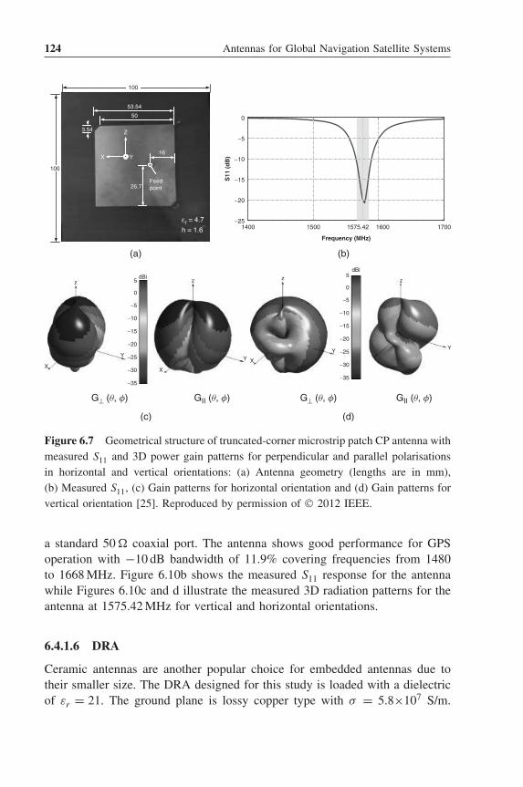
124 Antennas for Global Navigation Satellite Systems
1400 1500 1575.42 1600 1700−25
−20
−15
−10
−5
0
Frequency (MHz)
S11
(d
B)
100
53.54
50
16
26.7Feedpoint
εr = 4.7
h = 1.6
3.54 Z
X Y
100
z z z
YY X
Y
z
Y
XX
dBi5
0
−5
−10
−15
−20
−25
−30
−35
dBi5
0
−5
−10
−15
−20
−25
−30
−35
(a) (b)
G⊥ (q, f) GII (q, f) GII (q, f)G⊥ (q, f)
(c) (d)
Figure 6.7 Geometrical structure of truncated-corner microstrip patch CP antenna withmeasured S11 and 3D power gain patterns for perpendicular and parallel polarisationsin horizontal and vertical orientations: (a) Antenna geometry (lengths are in mm),(b) Measured S11, (c) Gain patterns for horizontal orientation and (d) Gain patterns forvertical orientation [25]. Reproduced by permission of © 2012 IEEE.
a standard 50 � coaxial port. The antenna shows good performance for GPSoperation with −10 dB bandwidth of 11.9% covering frequencies from 1480to 1668 MHz. Figure 6.10b shows the measured S11 response for the antennawhile Figures 6.10c and d illustrate the measured 3D radiation patterns for theantenna at 1575.42 MHz for vertical and horizontal orientations.
6.4.1.6 DRA
Ceramic antennas are another popular choice for embedded antennas due totheir smaller size. The DRA designed for this study is loaded with a dielectricof εr = 21. The ground plane is lossy copper type with σ = 5.8×10⁷ S/m.
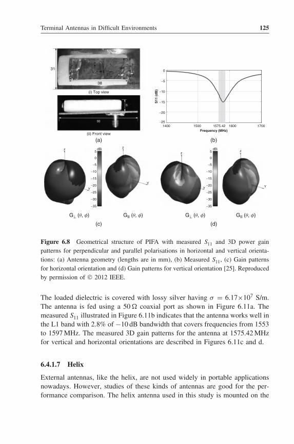
Terminal Antennas in Difficult Environments 125
1400 1500 1575.42 1600 1700−25
−20
−15
−10
−5
0
Frequency (MHz)
S11
(d
B)
31
38
(i) Top view
(ii) Front view
(a) (b)
(c) (d)
z z
z
Y Y
Y
z
Y
dBi5
0
−5
−10
−15
−20
−25
−30
−35
dBi5
0
−5
−10
−15
−20
−25
−30
−35
G⊥ (q, f) G⊥ (q, f)GII (q, f) GII (q, f)
Figure 6.8 Geometrical structure of PIFA with measured S11 and 3D power gainpatterns for perpendicular and parallel polarisations in horizontal and vertical orienta-tions: (a) Antenna geometry (lengths are in mm), (b) Measured S11, (c) Gain patternsfor horizontal orientation and (d) Gain patterns for vertical orientation [25]. Reproducedby permission of © 2012 IEEE.
The loaded dielectric is covered with lossy silver having σ = 6.17×10⁷ S/m.The antenna is fed using a 50 � coaxial port as shown in Figure 6.11a. Themeasured S11 illustrated in Figure 6.11b indicates that the antenna works well inthe L1 band with 2.8% of −10 dB bandwidth that covers frequencies from 1553to 1597 MHz. The measured 3D gain patterns for the antenna at 1575.42 MHzfor vertical and horizontal orientations are described in Figures 6.11c and d.
6.4.1.7 Helix
External antennas, like the helix, are not used widely in portable applicationsnowadays. However, studies of these kinds of antennas are good for the per-formance comparison. The helix antenna used in this study is mounted on the
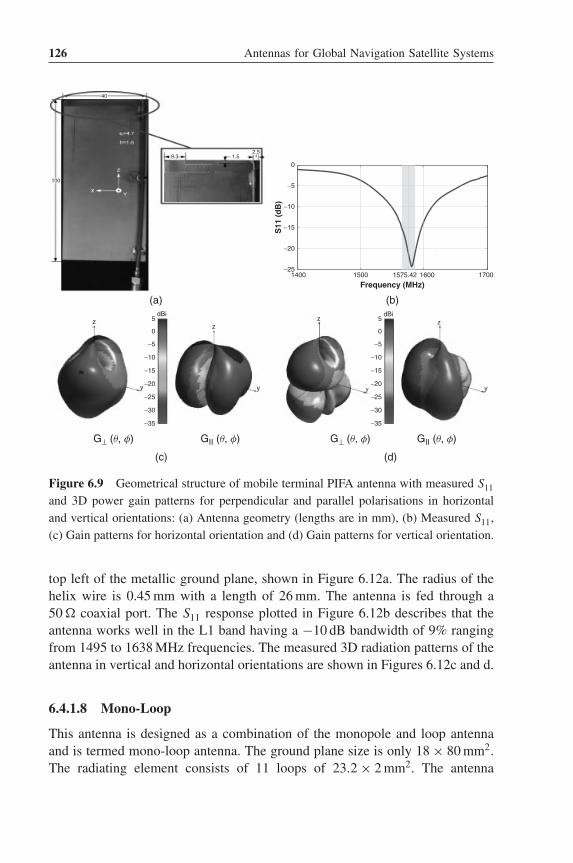
126 Antennas for Global Navigation Satellite Systems
1400 1500 1575.42 1600 1700−25
−20
−15
−10
−5
0
Frequency (MHz)S
11 (
dB
)
(a) (b)
G⊥ (q, f) GII (q, f) GII (q, f)G⊥ (q, f)
(c) (d)
100
y y y y
x x
zz
z zdBi
5
0
−5
−10
−15
−25
−20
−30
−35
dBi5
0
−5
−10
−15
−25
−20
−30
−35
40
9.3 1.52.5
Figure 6.9 Geometrical structure of mobile terminal PIFA antenna with measured S11
and 3D power gain patterns for perpendicular and parallel polarisations in horizontaland vertical orientations: (a) Antenna geometry (lengths are in mm), (b) Measured S11,(c) Gain patterns for horizontal orientation and (d) Gain patterns for vertical orientation.
top left of the metallic ground plane, shown in Figure 6.12a. The radius of thehelix wire is 0.45 mm with a length of 26 mm. The antenna is fed through a50 � coaxial port. The S11 response plotted in Figure 6.12b describes that theantenna works well in the L1 band having a −10 dB bandwidth of 9% rangingfrom 1495 to 1638 MHz frequencies. The measured 3D radiation patterns of theantenna in vertical and horizontal orientations are shown in Figures 6.12c and d.
6.4.1.8 Mono-Loop
This antenna is designed as a combination of the monopole and loop antennaand is termed mono-loop antenna. The ground plane size is only 18 × 80 mm2.The radiating element consists of 11 loops of 23.2 × 2 mm2. The antenna

Terminal Antennas in Difficult Environments 127
(a) (b)
G⊥ (q, f) GII (q, f) GII (q, f)G⊥ (q, f)
(c) (d)
yy
x
dBi5
0
−5
−10
−15
−25
−20
−30
−35
dBi5
0
−5
−10
−15
−25
−20
−30
−35
z z zz
y y
1400 1500 1575.42 1600 1700−50
−40
−30
−20
−10
0
Frequency (MHz)
S11
(d
B)
Figure 6.10 Geometrical structure of IFA antenna with measured S11 and 3D powergain patterns for perpendicular and parallel polarisations in horizontal and verticalorientations: (a) Antenna geometry (lengths are in mm), (b) Measured S11, (c) Gainpatterns for horizontal orientation and (d) Gain patterns for vertical orientation.
exhibits a −10 dB impedance bandwidth of 107 MHz covering the frequenciesfrom 1520 to 1627 MHz. Figure 6.13a illustrates the geometrical structure andFigure 6.13b shows the measured S11 curve for the antenna. Figures 6.13cand d depict the measured 3D patterns for the antenna.
6.4.2 Comparison Based on Simulated and Measured 3DRadiation Patterns
Firstly, statistical calculation results of the model are compared for two dif-ferent input methods. The three generic antennas, namely dipole, CP patchand generic PIFA, are analysed in the open field multipath environment tobenchmark the working of the proposed model. The 3D gain patterns of thethree antennas obtained through the simulations and the anechoic chamber(Satimo Stargate 64) measurements are used for the comparison. The results
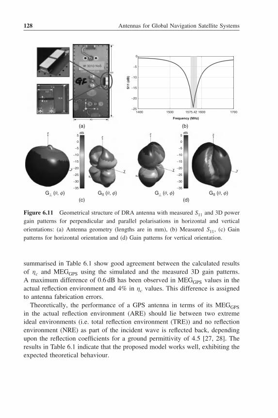
128 Antennas for Global Navigation Satellite Systems
(a) (b)
G⊥ (q, f) GII (q, f) GII (q, f)G⊥ (q, f)(c) (d)
y yy
xx
y
zzz
z dBi5
0
−5
−10
−15
−25
−20
−30
−35
dBi5
0
−5
−10
−15
−25
−20
−30
−35
1400 1500 1575.42 1600 1700−25
−20
−15
−10
−5
0
Frequency (MHz)
S11
(d
B)
Figure 6.11 Geometrical structure of DRA antenna with measured S11 and 3D powergain patterns for perpendicular and parallel polarisations in horizontal and verticalorientations: (a) Antenna geometry (lengths are in mm), (b) Measured S11, (c) Gainpatterns for horizontal orientation and (d) Gain patterns for vertical orientation.
summarised in Table 6.1 show good agreement between the calculated resultsof ηc and MEGGPS using the simulated and the measured 3D gain patterns.A maximum difference of 0.6 dB has been observed in MEGGPS values in theactual reflection environment and 4% in ηc values. This difference is assignedto antenna fabrication errors.
Theoretically, the performance of a GPS antenna in terms of its MEGGPSin the actual reflection environment (ARE) should lie between two extremeideal environments (i.e. total reflection environment (TRE)) and no reflectionenvironment (NRE) as part of the incident wave is reflected back, dependingupon the reflection coefficients for a ground permittivity of 4.5 [27, 28]. Theresults in Table 6.1 indicate that the proposed model works well, exhibiting theexpected theoretical behaviour.

Terminal Antennas in Difficult Environments 129
(a) (b)
G⊥ (q, f) GII (q, f) GII (q, f)G⊥ (q, f)(c) (d)
dBi5
0
−5
−10
−15
−25
−20
−30
−35
dBi5
0
−5
−10
−15
−25
−20
−30
−35
zz
yy y y
x
z z
1400 1500 1575.42 1600 1700−50
−40
−30
−20
−10
0
Frequency (MHz)S
11 (
dB
)
Figure 6.12 Geometrical structure of helix antenna with measured S11 and 3D powergain patterns for perpendicular and parallel polarisations in horizontal and verticalorientations: (a) Antenna geometry (lengths are in mm), (b) Measured S11, (c) Gainpatterns for horizontal orientation and (d) Gain patterns for vertical orientation.
6.4.3 Comparison Based on Measured 3D Radiation Patternsand Actual Field Tests
The comparison of the model’s calculations to open field measurements servesas a crucial step in the validation process. The horizontal dipole antenna is usedas a reference antenna in this study. Both the calculated (obtained throughthe proposed model using 3D measured gain patterns) and measured (meanSNR level observed in the actual field test) values of MEGGPS are normalisedto the corresponding values for the horizontal dipole antenna and describedin dBd. Hence, −5.4 dB (in the actual reflection environment given in Table 6.1)

130 Antennas for Global Navigation Satellite Systems
(a) (b)
G⊥ (q, f) GII (q, f) GII (q, f)G⊥ (q, f)(c) (d)
dBi5
0
−5
−10
−15
−25
−20
−30
−35
dBi5
0
−5
−10
−15
−25
−20
−30
−35
z z
y y y y
z
z
x
1400 1500 1575.42 1600 1700−25
−20
−15
−10
−5
0
Frequency (MHz)
S11
(d
B)
Figure 6.13 Geometrical structure of mono-loop antenna with measured S11 and 3Dpower gain patterns for perpendicular and parallel polarisations in horizontal and verticalorientations: (a) Antenna geometry (lengths are in mm), (b) Measured S11, (c) Gainpatterns for horizontal orientation and (d) Gain patterns for vertical orientation.
Table 6.1 Comparison of calculated ηc and MEGGPS of tested GPS antennas indifferent reflection environments using simulated and measured 3D power gainpatterns for validation of proposed GPS multipath model (TRE = Total ReflectionEnvironment, NRE = No Reflection Environment, ARE = Actual ReflectionEnvironment)
Antenna Model calculations using Model calculations usingsimulated 3D patterns measured 3D patterns
ηc (%) MEGGPS (dB) ηc (%) MEGGPS (dB)TRE NRE ARE TRE NRE ARE
Horizontal dipole 95 −3.2 −6.1 −5.2 97 −3.7 −6.4 −5.4Horizontal CP patch 100 −5.2 −5.7 −5.4 99 −5.8 −6.2 −6.0Horizontal PIFA 98 −4.0 −5.8 −4.6 94 −4.3 −6.3 −5.1

Terminal Antennas in Difficult Environments 131
and 40.2 dB (in the open field test) are being used as the reference levelsfor the calculated and measured results, respectively. The antennas are placedhorizontally with respect to the ground. The results are summarised in Table 6.2.
In these assessments, the repeatability of the measurement procedure mustalso be known. Therefore, in these as well as the following investigations,MEGGPS and ηc are calculated performing three sets of measurements for eachantenna and reporting the mean values. The standard deviation of these threemeasurements (averaged over various tested scenarios) is 0.6 dB and 5% forMEGGPS and ηc, respectively.
Table 6.2 Comparison of calculated ηc and MEGGPS of tested GPS antennas inhorizontal and vertical orientations using measured 3D power gain patterns with theactual field test measurements
Antenna Orientation Model calculations using Open fieldmeasured 3D patterns test measurements
ηc(%) MEGGPS(dBd) ηc(%) MEGGPS(dBd)
Dipole Horizontal 97 0 (correspondingto calculatedvalue of −5.4dB in ARE)
96 0 (correspondingto measuredaverage SNR of40.2 dB)
Vertical 94 −0.2 92 −0.2
CP patch Horizontal 99 −0.6 97 −0.4Vertical 72 −2.1 72 −2.2
Generic PIFA Horizontal 94 0.3 94 0.2Vertical 97 −0.5 97 −0.8
Terminal PIFA Horizontal 83 −2.2 81 −2.3Vertical 95 −3.3 92 −3.1
IFA Horizontal 100 0.6 97 0.4Vertical 79 −0.4 81 −0.3
DRA Horizontal 95 −0.6 94 −0.5Vertical 94 −0.5 90 −0.5
Helix Horizontal 97 −1.2 96 −1.5Vertical 87 −0.6 87 −1.0
Mono-loop Horizontal 80 −2.0 82 −1.6Vertical 78 −1.6 80 −1.8

132 Antennas for Global Navigation Satellite Systems
(b)
70
80
90
100
IFA
CP Pat
ch
Dipole
Helix
DRA
PIFA (G
ener
ic)
PIFA (T
erm
inal)
Mon
oloop
Antenna under test
hc
(%)
CalculatedMeasured
−4
−3
−2
−1
0
1
IFA
CP Patc
h
Dipole
Helix
DRA
PIFA (G
ener
ic)
PIFA (T
ermina
l)
Mono-
loop
Antenna under test
ME
GG
PS (
dB
d)
CalculatedMeasured
(a)
Figure 6.14 Comparison of calculated and measured values of MEGGPS and ηc show-ing performance ranking of GPS antennas in horizontal orientation: (a) MEGGPS takinghorizontal dipole as a reference (0 dBd); (b) ηc.
The field test results show good agreement with the model’s predictions forMEGGPS and ηc values for the mobile terminal GPS antennas. Figure 6.14indicates that a similar performance ranking of the tested antennas has beenachieved in both the calculations and measurements. It confirms that the modelcan successfully translate and predict the working of GPS antennas in a mul-tipath environment. A maximum difference of 0.4 dB is noted for MEGGPSvalues and 3% for ηc values between the model’s calculations and open field

Terminal Antennas in Difficult Environments 133
measurements. These differences are well below the accepted levels reportedin the literature [1, 2, 5]. They are mainly attributed to random factors arisingfrom atmospheric errors and weather conditions.
The results also indicate that the two parameters of MEGGPS and ηc do notrely greatly on each other. An antenna with good ηc may exhibit poor MEGGPSand vice versa, for example in the case of the generic PIFA antenna. However,the multipath performance of GPS antennas could only be characterised bya combined consideration of the two parameters. MEGGPS incorporates thewhole environment taking into account both the direct and multipath signals,especially the ground reflections. On the other hand, ηc only considers thedirect link. An antenna having low values of MEGGPS and ηc would be unableto establish a quick GPS link as the direct signal is weak while the multipathimpact is less significant. The performance of the antenna with high values ofMEGGPS should be analysed further in terms of its ηc. A high ηc shows thatthe direct signal is stronger than the multipath signal enabling the antenna toachieve an overall good performance with quick GPS link and low multipatherrors. On the contrary, low ηc shows a weaker direct signal with a greaterimpact of the multipath signal. An antenna exhibiting such a performancecould build satellite link quickly but with high errors. The CP patch and IFAbelong to the first category while the generic PIFA lies in the second category.However, an optimal performance could only be achieved with an antennaexhibiting good MEGGPS and ηc.
6.5 Performance Dependence on GNSS Antenna Orientation
Antenna orientation plays a vital role in multipath wireless communication.Varying orientation changes the antenna main lobe direction inflictinglink losses. The mobile terminals operate in a dynamic environment withever-changing orientations of the antennas depending on the user’s holdingposition. The effects of these changes on mobile terminal GPS antennas ischaracterised in this section. The antennas are placed in a vertical orientation(with respect to the ground) and performance is studied in comparison withthe horizontal orientations.
The calculated and measured results using the proposed statistical model andopen field test are presented in Table 6.2. Figure 6.15 shows the comparisonof the antenna rankings in terms of their MEGGPS and ηc based on the twomethods. It is further established that the model delivers precise results with aclose agreement to the field test observations. A maximum relative differenceof 0.4 dB in MEGGPS and 4% in ηc has been noted.
These results also show that change in the antenna orientation has a profoundeffect on the performance of GPS antennas. Comparing the vertically oriented
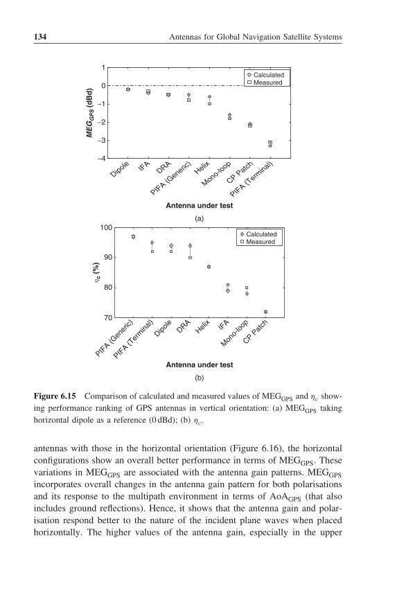
134 Antennas for Global Navigation Satellite Systems
−4
−3
−2
−1
0
1
Dipole IFADRA
PIFA (Generic
)Helix
Mono-loop
CP Patch
PIFA (Term
inal)
Antenna under test
ME
GG
PS (
dB
d)
CalculatedMeasured
(a)
CalculatedMeasured
(b)
70
80
90
100
PIFA (G
ener
ic)
PIFA (T
erm
inal)
Dipole
DRAHeli
xIF
A
Mon
o-loo
p
CP Pat
ch
Antenna under test
hc
(%)
Figure 6.15 Comparison of calculated and measured values of MEGGPS and ηc show-ing performance ranking of GPS antennas in vertical orientation: (a) MEGGPS takinghorizontal dipole as a reference (0 dBd); (b) ηc.
antennas with those in the horizontal orientation (Figure 6.16), the horizontalconfigurations show an overall better performance in terms of MEGGPS. Thesevariations in MEGGPS are associated with the antenna gain patterns. MEGGPSincorporates overall changes in the antenna gain pattern for both polarisationsand its response to the multipath environment in terms of AoAGPS (that alsoincludes ground reflections). Hence, it shows that the antenna gain and polar-isation respond better to the nature of the incident plane waves when placedhorizontally. The higher values of the antenna gain, especially in the upper

Terminal Antennas in Difficult Environments 135
−4
−3
−2
−1
0
1
Dipole
CP Patc
h
PIFA (G
ener
ic)
PIFA (T
ermina
l)IF
ADRA
Helix
Mono-
loop
Antenna under test
ME
GG
PS (
dB
d)
HorizontalVertical
(a)
Antenna under test
0
20
40
60
80
10
Dipole
CP Patc
h
PIFA(G
ener
ic)DRA
IFA
PIFA (T
ermina
l)Heli
x
Mono-
loop
hc
(%)
HorizontalVertical
(b)
Figure 6.16 Performance comparison of GPS antennas with effects of change inorientation in terms of calculated MEGGPS (taking horizontal dipole as reference) andηc: (a) MEGGPS taking horizontal dipole as a reference (0 dBd); (b) ηc.
hemispherical space, in both the perpendicular and parallel polarisations (aspresented in the gain pattern figures), are a key contributor.
The majority of the tested antennas including the CP patch, IFA and helixalso exhibit better ηc in the horizontal orientation as more open sky view isavailable. It increases the number of tracked satellites and hence the level of thereceived signal in the incident region (0◦ ≤ θ ≤ 90◦). As a result, the wastedsignal is reduced, improving the overall ηc. The change in antenna ηc withchanging orientation (with respect to the ground) is attributed to the sensitivity

136 Antennas for Global Navigation Satellite Systems
of the antenna to receive the incoming GPS signal. Since the incoming GPSsignal is RHCP, antenna RHCP gain patterns are evaluated in order to studythe relation between ηc and RHCP gain with change in antenna orientation.The RHCP gain patterns of the tested antennas are measured using Satimo’sStargate 64 measurement system. Figures 6.17 and 6.18 present the comparisonof measured RHCP gains in the incident region for the tested antennas in boththe horizontal and vertical orientations. In these figures, the cross-hatched areaindicates useful angles having a gain level above −13 dBi, contributing to ηc.
The comparison of the presented plots clearly indicates that ηc of the antennadepends upon the strength of the RHCP gain in the incident region. Forexample, in the case of the CP patch antenna, the vertical orientation exhibitsmuch lower ηc of 72% compared with 99% for the horizontal orientation. Itshows that the antenna has more clear sky view and a larger coverage areawhen placed horizontally. The RHCP gain patterns also support this theory.Figure 6.17b(i) shows that all of the incident region is above the requiredthreshold level of −13 dBi when the antenna is working in the horizontal ori-entation. A decreased ηc for the vertically orientated antenna is caused bycomparatively less area meeting this threshold. The presence of the RHCP gainlevels lower than −13 dBi (non-hatched area) in Figure 6.17b(ii), particularly inthe angles 30◦ ≤ θ ≤ 90◦, 0◦ ≤ φ ≤ 60◦ and 40◦ ≤ θ ≤ 90◦, 330◦ ≤ φ ≤ 360◦,gives rise to wasted signals resulting in a lower ηc. Similarly, ηc of the hori-zontal IFA is 100% but only 79% for the vertical IFA. The RHCP gain patternsin Figure 6.18a(ii) illustrate that the whole incident region fulfils the −13 dBithreshold for the horizontal orientation while a wide area in 30◦ ≤ θ ≤ 90◦,0◦ ≤ φ ≤ 140◦ fails to meet this criterion for the vertical orientation. Similarbehaviour could be observed for the helix antenna.
The tested antennas can be divided into three groups. The first group showsa tendency of improved MEGGPS with enhanced ηc and vice versa on vary-ing orientation. The dipole, CP patch and IFA come under this group. Inthe second group, if MEGGPS increases, ηc decreases and vice versa. Thegeneric PIFA, mobile terminal PIFA, helix and mono-loop antennas exhibitsuch behaviour. The third group consists of the antennas that have little impactof the changing orientation on their MEGGPS and ηc. The DRA shows thisstable performance.
It has been observed that the CP patch is more vulnerable to change in theorientation as MEGGPS and ηc vary significantly. The vertical CP patch has lost1.6 dB of its MEGGPS and 27% of its coverage compared with the horizontalCP patch. This indicates that the multipath signal has little impact upon theCP patch antenna and it relies more on the direct signal lowering its capabilityto establish a quick satellite link in arbitrary orientations. The performance of

Terminal Antennas in Difficult Environments 137
Gain (dBi)5 0 −5 −10 −15 −20 −25 −30 −35
Th
eta
(deg
rees
)
90
60
30
00 45 90 135 180 225 270 315 360
Phi (degrees)
Th
eta
(deg
rees
)
90
60
30
00 45 90 135 180 225 270 315 360
Phi (degrees)
(i) Horizontal orientation (ii) Vertical orientation
Th
eta
(deg
rees
)
90
60
30
00 45 90 135 180 225 270 315 360
Phi (degrees)
Th
eta
(deg
rees
)
90
60
30
00 45 90 135 180 225 270 315 360
Phi (degrees)
(i) Horizontal orientation (ii) Vertical orientation
(a)
Th
eta
(deg
rees
)
90
60
30
00 45 90 135 180 225 270 315 360
Phi (degrees)
Th
eta
(deg
rees
)
90
60
30
00 45 90 135 180 225 270 315 360
Phi (degrees)
(i) Horizontal orientation (ii) Vertical orientation
Th
eta
(deg
rees
)
90
60
30
00 45 90 135 180 225 270 315 360
Phi (degrees)
Th
eta
(deg
rees
)
90
60
30
00 45 90 135 180 225 270 315 360
Phi (degrees)
(i) Horizontal orientation (ii) Vertical orientation
(c)
(d)
(b)
Figure 6.17 Measured RHCP gain patterns in the incident region for dipole, CP patch,PIFA (generic) and PIFA (terminal) GPS antennas in horizontal and vertical orientations(cross-hatched regions indicate where signal is above −13 dBi): (a) Dipole, (b) CPPatch, (c) PIFA (Generic) and (d) PIFA (Terminal) [25]. Reproduced by permission of© 2012 IEEE.

138 Antennas for Global Navigation Satellite Systems
Gain (dBi)5 0 −5 −10 −15 −20 −25 −30 −35
Th
eta
(deg
rees
)
90
60
30
00 45 90 135 180 225 270 315 360
Phi (degrees)
Th
eta
(deg
rees
)
90
60
30
00 45 90 135 180 225 270 315 360
Phi (degrees)
(i) Horizontal orientation (ii) Vertical orientation
Th
eta
(deg
rees
)
90
60
30
00 45 90 135 180 225 270 315 360
Phi (degrees)
Th
eta
(deg
rees
)90
60
30
00 45 90 135 180 225 270 315 360
Phi (degrees)
(i) Horizontal orientation (ii) Vertical orientation
(a)
Th
eta
(deg
rees
)
90
60
30
00 45 90 135 180 225 270 315 360
Phi (degrees)
Th
eta
(deg
rees
)
90
60
30
00 45 90 135 180 225 270 315 360
Phi (degrees)
(i) Horizontal orientation (ii) Vertical orientation
Th
eta
(deg
rees
)
90
60
30
00 45 90 135 180 225 270 315 360
Phi (degrees)
Th
eta
(deg
rees
)
90
60
30
00 45 90 135 180 225 270 315 360
Phi (degrees)
(i) Horizontal orientation (ii) Vertical orientation
(c)
(d)
(b)
Figure 6.18 Measured RHCP gain patterns in the incident region for IFA, DRA, helixand mono-loop GPS antennas in horizontal and vertical orientations (cross-hatchedregions indicate where signal is above −13 dBi): (a) IFA, (b) DRA, (c) Helix and (d)Mono-loop.
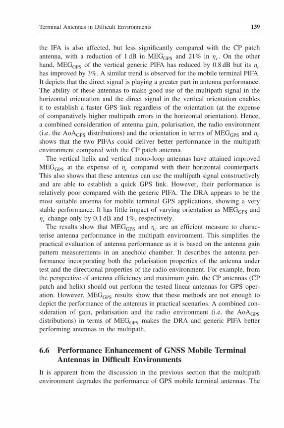
Terminal Antennas in Difficult Environments 139
the IFA is also affected, but less significantly compared with the CP patchantenna, with a reduction of 1 dB in MEGGPS and 21% in ηc. On the otherhand, MEGGPS of the vertical generic PIFA has reduced by 0.8 dB but its ηc
has improved by 3%. A similar trend is observed for the mobile terminal PIFA.It depicts that the direct signal is playing a greater part in antenna performance.The ability of these antennas to make good use of the multipath signal in thehorizontal orientation and the direct signal in the vertical orientation enablesit to establish a faster GPS link regardless of the orientation (at the expenseof comparatively higher multipath errors in the horizontal orientation). Hence,a combined consideration of antenna gain, polarisation, the radio environment(i.e. the AoAGPS distributions) and the orientation in terms of MEGGPS and ηc
shows that the two PIFAs could deliver better performance in the multipathenvironment compared with the CP patch antenna.
The vertical helix and vertical mono-loop antennas have attained improvedMEGGPS at the expense of ηc compared with their horizontal counterparts.This also shows that these antennas can use the multipath signal constructivelyand are able to establish a quick GPS link. However, their performance isrelatively poor compared with the generic PIFA. The DRA appears to be themost suitable antenna for mobile terminal GPS applications, showing a verystable performance. It has little impact of varying orientation as MEGGPS andηc change only by 0.1 dB and 1%, respectively.
The results show that MEGGPS and ηc are an efficient measure to charac-terise antenna performance in the multipath environment. This simplifies thepractical evaluation of antenna performance as it is based on the antenna gainpattern measurements in an anechoic chamber. It describes the antenna per-formance incorporating both the polarisation properties of the antenna undertest and the directional properties of the radio environment. For example, fromthe perspective of antenna efficiency and maximum gain, the CP antennas (CPpatch and helix) should out perform the tested linear antennas for GPS oper-ation. However, MEGGPS results show that these methods are not enough todepict the performance of the antennas in practical scenarios. A combined con-sideration of gain, polarisation and the radio environment (i.e. the AoAGPSdistributions) in terms of MEGGPS makes the DRA and generic PIFA betterperforming antennas in the multipath.
6.6 Performance Enhancement of GNSS Mobile TerminalAntennas in Difficult Environments
It is apparent from the discussion in the previous section that the multipathenvironment degrades the performance of GPS mobile terminal antennas. The

140 Antennas for Global Navigation Satellite Systems
time taken for the receiver to lock the GPS satellite (time to first fix (TTFF)) canreach up to 10 minutes, which is unacceptable for emergency calls. Provisionof a reliable navigation service demands mitigation of these degrading effects.The performance of the terminal antennas in a cluttered environment can beenhanced by employing different techniques including assisted GPS, GPS signalreradiation, beamforming and diversity antennas.
6.6.1 Assisted GPS
Assisted GPS, also termed A-GPS, is a system where external sources includ-ing an assistance server with greater computing power and reference networkprovide the GNSS receiver with aiding information. Precise information of theGPS satellite orbit, clock data, initial position and time estimate is providedby the assistance server that gets help from the reference network [33]. Theassistance server uses a wireless link to communicate with the GPS receiver.Provision of this data reduces the workload of the GPS receiver so it canoperate more quickly and efficiently with assistance from the network. TheTTFF can be decreased by a factor of 10, increasing the receiver’s sensitivity[34]. This system is employed in mobile telecommunication networks.However, it requires network access which is not always available and canalso compromise the user’s privacy.
6.6.2 GPS Signal Reradiation
This approach is based on the use of GPS repeaters. It consists of an outdoorGPS receiver antenna and an indoor GPS amplifier. The receiving antenna isplaced at a location where it has the best clear sky view, for example on theroof of a building or on a high pole. The GPS signal received outdoor bythe receiver antenna is then amplified and reradiated inside the premises. Theposition solution is calculated by the receiver inside the building relating tothe information obtained by the external antenna [35]. This method is a simpleand cost-effective solution for large shadowed areas with no access to the GPSsignal, including indoors and underground. However, the position of the indoorreceiver could always be the same, representing the location of the outdoorantenna. Furthermore, the regulatory bodies have placed special regulations onthe use of GPS repeaters to avoid signal jamming and interference with adjacentfrequency bands. The European Telecommunications Standards Institute (ETSI)limits the overall gain of the repeater to a maximum of 45 dB while the NationalTelecommunications and Information Administration (NTIA) and Ofcom forbidthe use of such devices (with the exception of specially permitted government
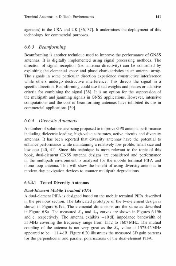
Terminal Antennas in Difficult Environments 141
agencies) in the USA and UK [36, 37]. It undermines the deployment of thistechnology for commercial purposes.
6.6.3 Beamforming
Beamforming is another technique used to improve the performance of GNSSantennas. It is digitally implemented using signal processing methods. Thedirection of signal reception (i.e. antenna directivity) can be controlled byexploiting the elemental space and phase characteristics in an antenna array.The signals in some particular direction experience constructive interferencewhile others undergo destructive interference. This directs the signal in aspecific direction. Beamforming could use fixed weights and phases or adaptivecriteria for combining the signal [38]. It is an option for the suppression ofthe multipath and jamming signals in GNSS applications. However, intensivecomputations and the cost of beamforming antennas have inhibited its use incommercial applications [39].
6.6.4 Diversity Antennas
A number of solutions are being proposed to improve GPS antenna performanceincluding dielectric loading, high-value substrates, active circuits and diversityantennas. It has been reported that diversity antennas have the potential toenhance performance while maintaining a relatively low profile, small size andlow cost [40, 41]. Since this technique is more relevant to the topic of thisbook, dual-element GNSS antenna designs are considered and performancein the multipath environment is analysed for the mobile terminal PIFA andmono-loop antenna. This will show the benefit of using diversity antennas inmodern-day navigation devices to counter multipath degradations.
6.6.4.1 Tested Diversity Antennas
Dual-Element Mobile Terminal PIFAA dual-element PIFA is designed based on the mobile terminal PIFA describedin the previous section. The fabricated prototype of the two-element design isshown in Figure 6.19a. The elemental dimensions are the same as describedin Figure 6.9a. The measured S11 and S21 curves are shown in Figures 6.19band c, respectively. The antenna exhibits −10 dB impedance bandwidth of55 MHz covering the frequency range from 1552 to 1607 MHz. The mutualcoupling of the antenna is not very great as the S21 value at 1575.42 MHzappeared to be −11.4 dB. Figure 6.20 illustrates the measured 3D gain patternsfor the perpendicular and parallel polarisations of the dual-element PIFA.

142 Antennas for Global Navigation Satellite Systems
(a)
1400 1500 1575.421600 1700−25
−20
−15
−10
−5
0
Frequency (MHz)
S11
(d
B)
(b)
1400 1500 1575.42 1600 1700−25
−20
−15
−10
−5
0
Frequency (MHz)
S21
(d
B)
(c)
40
Figure 6.19 Geometrical structure of GPS mobile terminal dual-element PIFA diver-sity antenna with measured S11 and S21 curves: (a) Antenna geometry (lengths are inmm), (b) Measured S11 curve and (c) Measured S21 curve.
Dual-Element Mono-loop AntennaThe dual-element mono-loop antenna is also designed to study the enhancementof GPS antenna performance in the multipath environment using diversity [42].The elemental dimensions are similar, as illustrated in Figure 6.13a, with a dis-tance of 41.8 mm between the two elements. Figure 6.21a shows the fabricatedprototype of the designed antenna while Figures 6.21b and c describe the mea-sured S11 and S21 curves respectively for the antenna. The antenna has a −10 dBimpedance bandwidth of 250 MHz covering all the frequencies ranging from1385 to 1635 MHz. An acceptable level of coupling between the two elementsis observed with the measured S21 of −14.1 dB at 1575.42 MHz. The measured
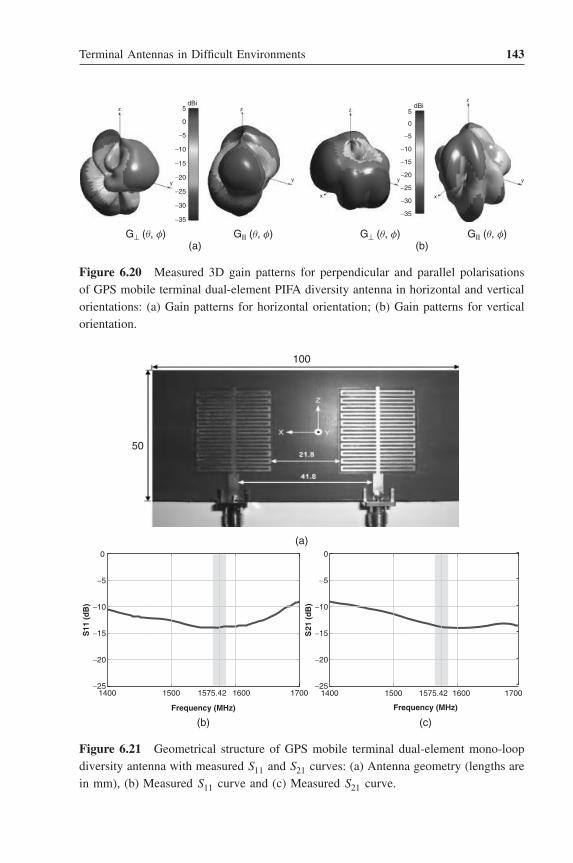
Terminal Antennas in Difficult Environments 143
G⊥ (q, f) GII (q, f) GII (q, f)G⊥ (q, f)(a) (b)
dBi5
0
−5
−10
−15
−25
−20
−30
−35
dBi5
0
−5
−10
−15
−25
−20
−30
−35
y
z
y y
z
y
x x
z
z
Figure 6.20 Measured 3D gain patterns for perpendicular and parallel polarisationsof GPS mobile terminal dual-element PIFA diversity antenna in horizontal and verticalorientations: (a) Gain patterns for horizontal orientation; (b) Gain patterns for verticalorientation.
(a)
100
50
1400 1500 1575.42 1600 1700−25
−20
−15
−10
−5
0
Frequency (MHz)
S11
(d
B)
1400 1500 1575.42 1600 1700−25
−20
−15
−10
−5
0
Frequency (MHz)
S21
(d
B)
(b) (c)
Figure 6.21 Geometrical structure of GPS mobile terminal dual-element mono-loopdiversity antenna with measured S11 and S21 curves: (a) Antenna geometry (lengths arein mm), (b) Measured S11 curve and (c) Measured S21 curve.

144 Antennas for Global Navigation Satellite Systems
G⊥ (q, f) GII (q, f) GII (q, f)G⊥ (q, f)(a) (b)
dBi5
0
−5
−10
−15
−25
−20
−30
−35
dBi5
0
−5
−10
−15
−25
−20
−30
−35
y
z
x
y y
z
y
zz
Figure 6.22 Measured 3D gain patterns for perpendicular and parallel polarisationsof GPS mobile terminal dual-element mono-loop diversity antenna in vertical and hor-izontal orientations: (a) Gain patterns for horizontal orientation; (b) Gain patterns forvertical orientation.
3D gain patterns for the perpendicular and parallel polarisations of the dual-element mono-loop antenna are illustrated in Figure 6.22.
6.6.4.2 Performance of GPS Diversity Antennas in MultipathEnvironment
The performance of the two diversity antennas in the multipath GPS environ-ment is evaluated using the proposed statistical model and verified throughopen field test measurements. A power combiner is used to combine the signalfrom the two elements with an insertion loss of 0.5 dB. The vertical orientationof the two antennas is taken into account. The 3D gain patterns of the antennaconfigurations are input to the model. The effectiveness of the diversity is anal-ysed in terms of ηc and MEGGPS with the horizontal dipole antenna taken asthe reference.
Table 6.3 summarises the MEGGPS and ηc results for the two antennas whilea comparison with the performance of respective single-element (non-diversity)antennas is presented in Figure 6.23.
Figure 6.23 shows that the use of the diversity antennas increases MEGGPSfor the GPS multipath operation significantly. The extent of this enhancementis different for the two antennas with a 0.6 dB increase achieved by the dual-element PIFA while a 1.4 dB increase is offered by the dual-element mono-loop.
Similarly, a significant improvement in the coverage of the incoming GPSsignal has been exhibited by the dual-element mono-loop with an ηc incrementof 17%. The ηc of the dual-element PIFA has also increased by 2% which isnot very significant but shows a tendency of improvement.

Terminal Antennas in Difficult Environments 145
Table 6.3 Performance evaluation of mobile terminal GPS diversity antennas inhorizontal and vertical orientations using the multipath environment model incomparison with the measured results
Antenna Model calculations using Open fieldmeasured 3D patterns test measurements
ηc (%) MEGGPS (dBd) ηc (%) MEGGPS (dBd)
Horizontal dipole(reference)
97 0 (correspondingto calculatedvalue of −5.4dB in ARE)
96 0 (correspondingto measuredaverage SNR of40.2 dB)
Vertical terminal PIFA 95 −3.3 92 −3.1Vertical dual-terminal
PIFA97 −2.7 97 −2.6
Vertical mono-loop 78 −1.6 80 −1.8Vertical dual mono-loop 95 −0.2 96 −0.3
The higher values of MEGGPS and ηc achieved for the two diversity antennasare a result of enhanced gain patterns. The use of spatial diversity has broadenedthe antenna’s clear sky view, modified the gain patterns and increased the gainlevels as illustrated in Figures 6.20 and 6.22. The modified gain patterns haveenabled the antennas to cover a wider range of AoAGPS. This, combined withan overall increased gain level, has resulted in comparatively larger valuesof MEGGPS for the diversity antennas. The enhanced gain values have alsoincreased the coverage of the antennas and hence their ηc as this depends onthe solid angle subtended by the area where gain levels are higher than −13 dBiin the upper hemisphere. The results show that the diversity is good for themono-loop antenna but its benefit is marginal for the PIFA. The less resoundingperformance of the dual-element PIFA is related to fabrication errors that leadto higher mutual coupling between the two elements. The S21 measurements,presented in Figures 6.19c and 6.21c, show that the dual-element PIFA has amutual coupling of −11.4 dB as compared with −14.1 dB for the dual-elementmono-loop at 1575.42 MHz. It reduces the performance of the dual-elementPIFA to a greater extent resulting in less significant improvement in MEGGPSand ηc values compared with the dual-element mono-loop antenna.
Overall, the dual-element diversity antennas have shown better performancein the multipath environment compared with their single-element counterparts.It is therefore deduced that diversity is a viable solution in terms of effectiveGPS reception. Further optimisation of the antenna designs and minimisation

146 Antennas for Global Navigation Satellite Systems
PIFA(Terminal)
Mono-loop Dual PIFA DualMono-loop
−4
−3
−2
−1
0
Antenna under test
ME
GG
PS (
dB
d)
CalculatedMeasured
(a)
PIFA(Terminal)
Mono-loopDual PIFA DualMono-loop
0
20
40
60
80
100
Antenna under test
hc
(%)
CalculatedMeasured
(b)
Figure 6.23 Performance enhancement of GPS diversity antennas in multipath envi-ronment in comparison of single-element designs in terms of calculated MEGGPS (takingthe horizontal dipole as reference) and ηc: (a) MEGGPS taking horizontal dipole as areference (0 dBd); (b) ηc.
of the fabrication errors would result in more enhanced GPS operation of themobile terminal.
Besides its precise predictive capabilities, the proposed statistical model isonly suitable for open field (suburban) GPS environments due to the assump-tion of uniform AoAGPS in the azimuth and elevation planes. For urban areaoperation with a greater number of reflecting objects, more practical AoAGPS
representing a greater probability of arrival of the GPS signal near the zenithcompared with the horizon angles, for example Gaussian and elliptical distri-butions, should be considered.

Terminal Antennas in Difficult Environments 147
References1. Taga, T. “Analysis for mean effective gain of mobile antennas in land mobile radio environ-
ments”, IEEE Transactions on Vehicular Technology , 39, 117–131, 1990.2. Kalliola, K. Sulonen, K. Laitinen, H. et al. “Angular power distribution and mean effec-
tive gain of mobile antenna in different propagation environments”, IEEE Transactions onVehicular Technology , 51, 823–838, 2002.
3. Carro, P. and de Mingo, J. “Mean effective gain of compact WLAN genetic printed dipoleantennas in indoor-outdoor scenarios”, International Conference on Personal Wireless Com-munications (PWC), pp. 275–283, September 2006.
4. Ando, A. Taga, T. Kondo, A. Kagoshima, K. and Kubota, S. “Mean effective gain of mobileantennas in line-of-sight street microcells with low base station antennas”, IEEE Transactionson Antennas and Propagation , 56, 3552–3565, 2008.
5. Nielsen, J. and Pedersen, G. “Mobile handset performance evaluation using radiation patternmeasurements”, IEEE Transactions on Antennas and Propagation , 54, 2154–2165, 2006.
6. Krogerus, J. Ichelun, C. and Vainikainen, P. “Dependence of mean effective gain of mobileterminal antennas on side of head”, European Conference on Wireless Technology (ECWT),pp. 467–470, October 2005.
7. Axelrad, P. Comp, J. and MacDoran, P. “SNR-based multipath error correction for GPSdifferential phase”, IEEE Transactions on Aerospace and Electronic Systems , 32, 650–660,1996.
8. Wu, J. and Hsieh, C. “Statistical modeling for the mitigation of GPS multipath delays fromday-to-day range measurements”, Journal of Geodesy , 84, 223–232, 2006.
9. Spangenberg, M. Tourneret, J. Calmettes, V. and Duchteau, G. “Detection of variance changesand mean value jumps in measurement noise for multipath mitigation in urban navigation”,A silomar Conference on Signals, Systems and Computers P, October 2008.
10. Hannah, B. “Modelling and simulation of GPS multipath propagation”, PhD thesis, Queens-land University of Technology, March 2001.
11. Bancroft, R. Microstrip and printed antenna design , 2nd edn, SciTech Publishing, Raleigh,NC, 2009.
12. Moernaut, G. and Orban, D. “GNSS antennas: an introduction to bandwidth gain pattern,polarization and all that” GPS World , 20(2), 42–48, February 2009.
13. Boccia, L. Amendola, G. and Di Massa, G. “A shorted elliptical patch antenna for GPSapplications”, IEEE Antennas and Wireless Propagation Letters , 2, 6–8, 2003.
14. Miller, G. “Adding GPS applications to an existing design”, RF Design , pp. 50–57, March1998.
15. Langley, R. “A primer on GPS antennas”, GPS World , pp. 50–55, July 1998.16. Pathak, V. Thornwall, S. Krier, M. et al., “Mobile handset system performance comparison
of a linearly polarized GPS internal antenna with a circularly polarized antenna”, Antennasand Propagation Society International Symposium (AP-S), Vol. 3, June 2003.
17. Kingsley, S. “GPS antenna design for mobile phones”, Electronics Weekly , 11 April 2007.18. Haddrell, T. Ricquier, N. and Phocas, M. “Mobile-phone GPS antennas: can they be better?”,
GPS World , 21(2), 29–35, February 2010.19. Fujimoto, K. and James, J. R. Mobile antenna systems handbook , 2nd edn, Artech House,
Boston, MA, 2001.20. Chen, Z. N. Antennas for portable devices , John Wiley & Sons, Ltd, Chichester, 2007.21. Ur Rehman, M. Gao, Y. Chen, X. Parini, C. and Ying, Z. “Analysis of GPS antenna
performance in amultipath environment”, Antennas and Propagation Society InternationalSymposium (AP-S), July 2008.

148 Antennas for Global Navigation Satellite Systems
22. Ur Rehman, M. Gao, Y. Chen, X. Parini, C. and Ying, Z. “Environment effects and systemperformance characterisation of GPS antennas for mobile terminals”, IET Electronics Letters ,45, 243–245, 2009.
23. Ur Rehman, M. Gao, Y. Chen, X. Parini, C. and Ying, Z. “Characterisation of system per-formance of GPS antennas in mobile terminals including environmental effects”, EuropeanConference on Antennas and Propagation (EuCap), March 2009.
24. Jakes, W. Microwave mobile communications , John Wiley & Sons, Inc., New York, 1974.25. Ur Rehman, M. Chen, X. Parini, C. and Ying, Z. “Evaluation of statistical model for the
characterization of multipath affecting mobile terminal GPS antennas in sub-urban areas”,IEEE Tran. Antenna and Prop., Vol. 60, No. 2, 2012.
26. Cheng, D. Field and wave electromagnetics , 2nd edn, Addison-Wesley, Reading, MA, 1989.27. Jemai, J. Kurner, T. Varone, A. and Wagen, J. “Determination of the permittivity of build-
ing materials through WLAN measurements at 2.4GHz”, IEEE International Symposium onPersonal, Indoor and Mobile Radio Communications, September 2005.
28. Klysza, G. Balayssaca, J. and Ferriresb, X. “Evaluation of dielectric properties of concrete by anumerical FDTD model of a GPR coupled antennaparametric study”, NDT & E International ,41, 621–631, 2008.
29. J. Reed, Software radio: A modern approach to radio enginenering , Prentice-Hall, EnglewoodCliffs, NJ, 2002.
30. Tsui, J. Fundamentals of Global Positioning System Receivers: A software approach , 2nd edn,John Wiley & Sons, Inc., New York, 2000.
31. “Ultra low power superior sensitivity GPS modules”, URL http://www.starsnav.com/MTI-8T.htm (accessed 30 September 2011).
32. Pozar, D. Microwave engineering , 3rd edn, John Wiley & Sons, Inc., New York, 2005.33. Hoffmmann-Wellenhof, B. Lichtenegger, H. and Wasle, E. GNSS-Global navigation satellite
systems , Springer Vienna, 2008.34. Van Diggelen, F. S. T. A-GPS: Assisted GPS, GNSS, and SBAS , Artech House, London,
2009.35. Samama, N. Global positioning: Technologies and performance, John Wiley & Sons, Inc.,
Hoboken, NJ, 2008.36. ETSI, “EN 302645 draft on standardization of GNSS repeater”, http://www.etsi.org/deliver/
etsi_en/302600_302699/302645/01.01.01_20/en_302645v010101c.pdf (accessed 2 November2011).
37. NTIA, “Manual of regulations and procedures for federal radio frequency management”,http://www.ntia.doc.gov/files/ntia/publications/manual_5_11.pdf (accessed 2 November2011).
38. Kaplan, E. and Hegarty, C. Understanding GPS: Principles and applications , 2nd edn, ArtechHouse, London, 2005.
39. Fu, Z. Hornbostel, A. Hammesfahr, J. and Konovaltsev, A. “Suppression of multipath signalsby digital beamforming for GPS/Galileo applications”, GPS Solutions , 6 257, 2003.
40. Gao, Y. Chen, X. and Parini, C. G. “Study of diversity antennas for Galileo/GPS receivers”,European Navigation Conference (ENC-GNSS), April 2008.
41. Douglas, M. Okoniewski, M. and Stuchly, M. “A planar diversity antenna for handheld PCSdevices”, IEEE Transactions on Vehicular Technology , 47 747–754, 1998.
42. Ur Rehman, M. Gao, Y. Chen, X. and Parini, C. “Dual-element diversity antenna forGalileo/GPS receivers”, 13th World Congress of International Association of Institutes ofNavigation (IAIN), October 2009.

7Human User Effectson GNSS Antennas
7.1 Interaction of Human Body and GNSS Antennas
The GNSS devices in wireless body area networks (WPANs) and wirelesspersonal area networks (WBANs) typically operate either in on-body positions(held by the user) or in near-body positions (working in the proximity of thehuman body). In either case, the presence of the human body in the vicinitydegrades the performance of the embedded GPS antennas of such devices.
It is now a well-established phenomenon that the human body is a very lossymedium that affects the performance of the antenna in three ways: reduction inefficiency due to electromagnetic absorption in the tissues; degradation of theradiation pattern; and variation in the feed point impedance [1–7]. Characteri-sation of these effects is a challenging but necessary task to provide guidelinesfor the design of an optimal performance antenna resilient to these degradingfactors [8–11].
Following the land mobile antennas, the performance of GPS antennas alsotends to deteriorate when placed near the human body [12]. It increases themagnitude of degradations in the mobile terminal GPS antennas operating inthe multipath environment, that already have been suffering from reflections,diffraction and scattering of the incoming radio waves from surrounding objects[13, 14]. This results in attenuation, delay and distortion of the communicationlink. To guarantee a reliable navigation system that can also meet the FederalCommunications Commission’s (FCC’s) mandate E911 of provision of preciselocation of the mobile user to ensure public safety [15] requires that the GPS
Antennas for Global Navigation Satellite Systems, First Edition.Xiaodong Chen, Clive G. Parini, Brian Collins, Yuan Yao and Masood Ur Rehman.© 2012 John Wiley & Sons, Ltd. Published 2012 by John Wiley & Sons, Ltd.

150 Antennas for Global Navigation Satellite Systems
mobile terminal antennas should cope with these deteriorations. Therefore, theseantennas must be tested not only for the effects of the multipath environment,but also for the presence of the human body in this environment.
The effects of the human head presence in the multipath environment havebeen studied and reported in [16–18]. The mean effective gain (MEG) of theantenna is taken as a figure of merit for the antenna performance in these stud-ies. Since the calculations of antenna MEG are based on the antenna power gainpatterns, this simplifies antenna performance evaluation in practical scenariosincluding antenna on-body placements as follows [17,19–21]:
• The gain degradations due to radiation pattern deformations can be easilyaccommodated.
• The degradations of the antenna efficiency as a result of variations in theinput impedance can also be accounted for, irrespective of whether it iscaused by proximity of or absorptions by the human body.
The fast-growing demand for portable navigation devices necessitates theextension of this investigation to mobile terminal GPS antennas. The effects ofthe presence of the human body on the performance of GPS mobile terminalantennas is studied and characterised using the statistical model for the GPSmultipath environment discussed in Chapter 6.
7.2 Effects of Human Body on GNSS Mobile TerminalAntennas in Difficult Environments
The investigation is carried out using realistic numerical models of the humanhead, hand and the whole body to study the behaviour of various mobile ter-minal GPS antennas. The study is conducted in two parts: firstly, investigatingthe effects of the presence of the human head and hand; secondly, investigatingthe effects of the presence of the whole body in the vicinity of the antennas.Different possible on-body scenarios are investigated including antenna heldin user’s hand, antenna placed beside user’s head, antenna held in user’s handnear to the head in talking position and antenna placed at user’s pocket position.Effects of a multi-layered human head are also taken into account. The perfor-mance of GPS mobile terminal antennas is characterised in terms of MEGGPSand ηc. Since these parameters are calculated using simulated 3D power gainpatterns that only consider the power absorptions in human body tissues [22],it is essential to include the mismatch losses caused by the antenna detuningin these on-body configurations. These losses are accumulated in MEGGPS and

Human User Effects on GNSS Antennas 151
ηc employing the concept of ‘realised gain’, calculated using the followingequation [23]:
Gainrealised = Gain × ηm (7.1)
where Gain is the simulated gain that takes material losses into account. ηm rep-resents the antenna mismatch efficiency that accounts for the antenna detuninglosses and is calculated as follows:
ηm = 1 − |S11|2 (7.2)
CST Microwave Studio R© provides an embedded option for the realised gainmode [22].
7.2.1 Design of Tested GPS Antennas
Three types of GPS mobile terminal antennas are considered in this studyto investigate the human body effects. The three antennas include the PIFA,DRA and helix antenna and are similar in design as described in Chapter 5.The antennas operate at the GPS frequency of 1575.42 MHz. The PIFA isdesigned using an FR4 substrate of 1.6 mm thickness. The PCB size is 100 ×40 mm2. The DRA is loaded with a dielectric of εr = 21. The ground plane is100 × 40 mm2 of lossy copper type while the loaded dielectric is covered withlossy silver. The helix has no substrate and is mounted on the left side of themetallic ground plane of dimension 100 × 40 × 0.45 mm3. The PIFA and DRAare fed using discrete ports with 50 � impedance to represent the commonlyused 50 � coaxial port feed. Figures 7.1–7.3 show the schematic layout ofthe three antennas. The antenna prototypes were fabricated and tested in theAntenna Measurement Laboratory at Queen Mary University of London andresults have been reported in Chapter 6. In the current study, however, onlythe simulation results are of interest.
7.2.2 Effects of Human Hand and Head Presence
In the first part of the study, only the effects of the presence of a realistichuman head and hand model are investigated for the performance of GPSmobile terminal antennas in a multipath environment.
7.2.2.1 Test Set-up
A high-resolution realistic model of the human head and hand withdimensions for an average human is used as shown in Figure 7.4. The

152 Antennas for Global Navigation Satellite Systems
100
40
h=1.6
2.5 1.5 9.3
εr=4.7
Figure 7.1 Geometric structure of GPS mobile terminal PIFA used to study theeffects of human body presence on the antenna performance in a multipath environment(all lengths are in mm).
electrical properties of the muscle tissues are considered for the homogeneoushead and hand models at 1575.42 MHz with a permittivity of 53.86 andconductivity of 1.22 S/m [24–26]. An inhomogeneous multi-layer head modelis also employed to characterise the effects of different head tissues on theworking of the antenna. Five head tissues including skin, muscle, skull, brainand spinal cord are incorporated in this inhomogeneous model. Table 7.1summarises the electrical properties of these tissues at 1575.42 MHz andFigure 7.4e depicts a cross-sectional view of the multi-layer head modelwith anatomical details. An adaptive mesh is employed with different cellsizes that reduces the number of volume cells (voxels) in the computationaldomain significantly. The perfectly matched layer (PML) absorbing boundaryconditions [22] are used with a maximum cell size of 10 mm near the

Human User Effects on GNSS Antennas 153
100
40
h=1
1.3 1.3
0.5
3.27.4
10.9
Figure 7.2 Schematic layout of GPS mobile terminal DRA to study the effectsof human body presence on the antenna performance in a multipath environment(all lengths are in mm).
boundaries and a minimum size of 0.08 mm at the edges of the solids in thecomputational region.
Various on-body scenarios including the antennas placed beside thehomogeneous head, held in hand and held in hand near to the head intalking position are taken into consideration to investigate the added effectsof the human head and hand on antenna performance in the GPS multipathenvironment. The effects of the multi-layer head model in all the aboveconfigurations are then analysed. The antennas are placed beside the headinclined at 45◦ with respect to the z -axis for the talking positions. A separationof 10 mm between the antenna and the head is kept to allow clearance for themobile casing. The statistical analysis of antenna performance in the multipathenvironment in these on-body configurations needs information of the 3Dgain patterns in the perpendicular and parallel polarisations. Therefore, thesimulated 3D gain patterns for all the test set-ups are recorded.

154 Antennas for Global Navigation Satellite Systems
100
40
5.4
23
0.9
5.3
4.6
1
h=0.45
Figure 7.3 Geometry and dimensions of GPS mobile terminal helix antenna for thestudy of the presence of human body effects on the antenna performance in a multipathenvironment (all lengths are in mm).
7.2.2.2 Evaluation of GPS Antenna Performance
The S11 response of the three antennas is shown in Figures 7.5–7.7. Thesefigures confirm the well-known phenomenon of antenna detuning caused by thepresence of the human body. The amount of this detuning varies from antennato antenna. The most resilient antenna to this detuning effect has proved to bethe helix, which offered the required −10 dB bandwidth of ±5 MHz (desiredfor efficient GPS operation) in all the cases due to its wide bandwidth. TheS11 responses for the DRA (Figure 7.6) makes it the most sensitive of thethree tested antenna types to the human body effects. It has shown greaterdetuning than the PIFA and helix antenna, though losing −10 dB impedance
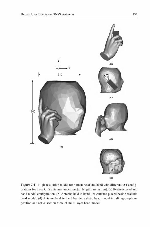
Human User Effects on GNSS Antennas 155
(b)
(a)
(c)
240
210
Y X
Z
45°
(e)
(d)
Figure 7.4 High-resolution model for human head and hand with different test config-urations for three GPS antennas under test (all lengths are in mm): (a) Realistic head andhand model configuration, (b) Antenna held in hand, (c) Antenna placed beside realistichead model, (d) Antenna held in hand beside realistic head model in talking-on-phoneposition and (e) X-section view of multi-layer head model.
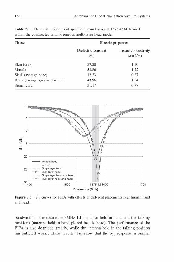
156 Antennas for Global Navigation Satellite Systems
Table 7.1 Electrical properties of specific human tissues at 1575.42 MHz usedwithin the constructed inhomogeneous multi-layer head model
Tissue Electric properties
Dielectric constant Tissue conductivity(εr ) (σ )(S/m)
Skin (dry) 39.28 1.10Muscle 53.86 1.22Skull (average bone) 12.33 0.27Brain (average grey and white) 43.96 1.04Spinal cord 31.17 0.77
1400 1500 1575.42 1600 170030
25
20
15
10
5
0
Frequency (MHz)
S11
(d
B)
Without bodyIn handSingle layer headMulti-layer headSingle layer head and handMulti-layer head and hand
Figure 7.5 S11 curves for PIFA with effects of different placements near human handand head.
bandwidth in the desired ±5 MHz L1 band for held-in-hand and the talkingpositions (antenna held-in-hand placed beside head). The performance of thePIFA is also degraded greatly, while the antenna held in the talking positionhas suffered worse. These results also show that the S11 response is similar

Human User Effects on GNSS Antennas 157
1400 1500 1575.421600 170030
25
20
15
10
5
0
Frequency (MHz)
S11
(d
B)
Without bodyIn handSingle layer headMulti-layer headSingle layer head and handMulti-layer head and hand
Figure 7.6 S11 curves for DRA with effects of different placements near human handand head.
1400 1500 1575.42 1600 170030
25
20
15
10
5
0
Frequency (MHz)
S11
(d
B)
Without body
In hand
Single layer head
Multi-layer head
Single layer head and hand
Multi-layer head and hand
Figure 7.7 S11 curves for helix with effects of different placements near human handand head.
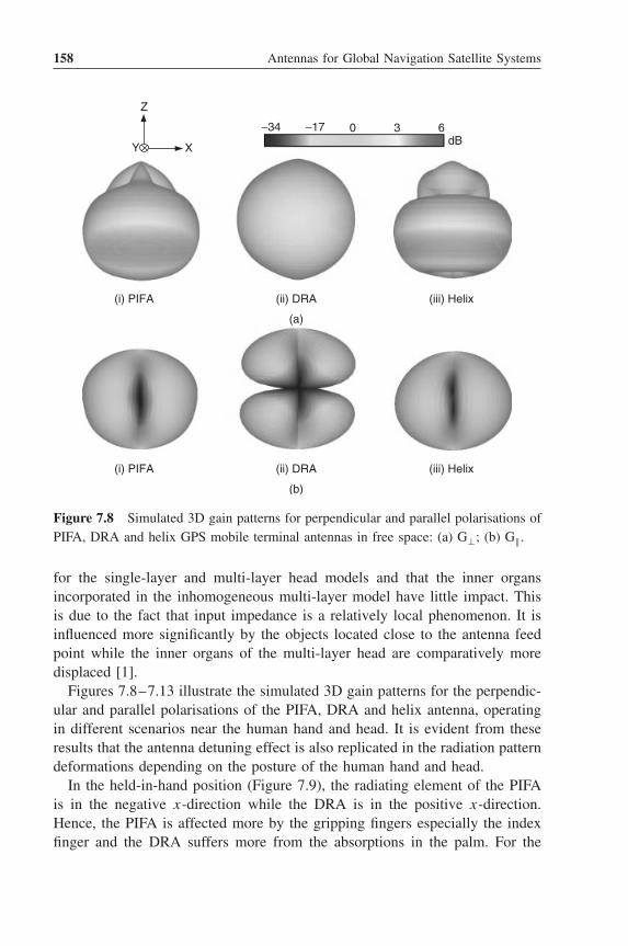
158 Antennas for Global Navigation Satellite Systems
X
Z
Y
−17 dB
6 0 3 −34
(i) PIFA (ii) DRA (iii) Helix
(a)
(i) PIFA (ii) DRA (iii) Helix
(b)
Figure 7.8 Simulated 3D gain patterns for perpendicular and parallel polarisations ofPIFA, DRA and helix GPS mobile terminal antennas in free space: (a) G⊥; (b) G‖.
for the single-layer and multi-layer head models and that the inner organsincorporated in the inhomogeneous multi-layer model have little impact. Thisis due to the fact that input impedance is a relatively local phenomenon. It isinfluenced more significantly by the objects located close to the antenna feedpoint while the inner organs of the multi-layer head are comparatively moredisplaced [1].
Figures 7.8–7.13 illustrate the simulated 3D gain patterns for the perpendic-ular and parallel polarisations of the PIFA, DRA and helix antenna, operatingin different scenarios near the human hand and head. It is evident from theseresults that the antenna detuning effect is also replicated in the radiation patterndeformations depending on the posture of the human hand and head.
In the held-in-hand position (Figure 7.9), the radiating element of the PIFAis in the negative x-direction while the DRA is in the positive x-direction.Hence, the PIFA is affected more by the gripping fingers especially the indexfinger and the DRA suffers more from the absorptions in the palm. For the

Human User Effects on GNSS Antennas 159
X
Z
Y
−17 dB
60 3−34
(i) PIFA (ii) DRA (iii) Helix
(a)
(i) PIFA (ii) DRA (iii) Helix
(b)
Figure 7.9 Simulated 3D gain patterns for perpendicular and parallel polarisationsof PIFA, DRA and helix GPS mobile terminal antennas held in user’s hand: (a) G⊥;(b) G‖.
helix in free space, the ground plane is a major contributor to the radiation.Therefore, it is also affected by the gripping fingers. When the antenna isplaced near the head, a greater body mass reduces the radiation of the threeantennas in the positive x-direction making the gain patterns directive inthe negative x-direction as shown in Figures 7.10 and 7.11. It can also beobserved from these results that gain levels are less in the upper hemispherecompared with the lower hemisphere. When the antenna is held in the user’shand in the talking position, the presence of both the hand and head on thetwo sides of the antenna give rise to electromagnetic absorptions and thereflected fields are minimum. This defragments the antenna radiation greatlyand causes poor gain levels in all directions, depicted in Figures 7.12–7.13.
The performance of the PIFA, DRA and helix GPS mobile terminal antennasin the multipath environment is evaluated using the discussed statistical modelin terms of MEGGPS and ηc. The simulated 3D gain patterns of the designed

160 Antennas for Global Navigation Satellite Systems
X
Z
Y
−17 dB
60 3 −34
(i) PIFA (ii) DRA (iii) Helix
(a)
(i) PIFA (ii) DRA (iii) Helix
(b)
Figure 7.10 Simulated 3D gain patterns for perpendicular and parallel polarisations ofPIFA, DRA and helix GPS mobile terminal antennas placed beside user’s homogeneoussingle-layer head: (a) G⊥; (b) G‖.
antennas in different configurations, shown in Figures 7.8–7.12, are input tothe model. The ground plane (earth) is considered as made of dry concrete witha relative permittivity of 4.5 [27, 28] to include the ground reflections.
Table 7.2 summarises the calculated values of ηc and MEGGPS for the threetested antennas in different near-body configurations. Note that the presence ofthe lossy human body tissues causes significant degradation of the antenna per-formance due to electromagnetic absorptions in the tissues and field reflectionsfrom the surface of the human body. This results in gain pattern deformationscompared with that without the presence of the human body, illustrated inFigures 7.9–7.13. This deterioration of the gain patterns reduces the coverageand MEGGPS of the GPS antennas and their ability to pick up the GPS satellitesignal suffers drastically.

Human User Effects on GNSS Antennas 161
(i) PIFA (ii) DRA (iii) Helix
(a)
X
Z
Y
−17 dB
6 0 3 −34
(i) PIFA (ii) DRA (iii) Helix
(b)
Figure 7.11 Simulated 3D gain patterns for perpendicular and parallel polarisationsof PIFA, DRA and helix GPS mobile terminal antennas positioned beside user’s inho-mogeneous multi-layer head: (a) G⊥; (b) G‖.
Note also that the reduction in ηc depends mainly on the extent of availableclear sky view to the radiating element. The more the antenna radiating elementis covered by the user, the lesser is its ηc. The amount of body mass presentin the vicinity of the GPS antenna also plays a key role.
Figure 7.14a compares the coverage of the three antennas in the abovedescribed test configurations. In the case of the PIFA, the radiating elementis in the negative x-direction. For the held-in-hand position, the radiating ele-ment (top edge of the PCB) is not covered by the palm or the gripping fingers.Only a small disturbance comes from the index finger resulting in ηc of 89%,that is 3% lower than the free space value. When the antenna is placed besidethe head, greater body volume produces larger detuning due to the surface

162 Antennas for Global Navigation Satellite Systems
X
Z
Y
−17 dB
6 0 3 −34
(i) PIFA (ii) DRA (iii) Helix
(a)
(i) PIFA (ii) DRA (iii) Helix
(b)
Figure 7.12 Simulated 3D gain patterns for perpendicular and parallel polarisationsof PIFA, DRA and helix GPS mobile terminal antennas held in user’s hand and placedbeside the user’s homogeneous single-layer head: (a) G⊥; (b) G‖.
reflections and energy absorptions and, hence, ηc decreases to 75%. Placingthe antenna in the talking position shields its clear sky view on both sides bythe user’s holding hand and head reducing the antenna’s coverage to 42%.
On the contrary, the radiating DRA is in the positive x-direction, located inthe middle of the PCB and, hence, affected more by the palm. The grippingfingers also cover most of the radiating element, resulting in a reduced ηc valueof 58% compared with the free space value of 95%. Placing the antenna besidethe head blocks its view only on one side, resulting in an ηc of 76%, but thepresence of both the hand and head shields most of the useful angles and,hence, ηc becomes 36%.
For the helix, the radiating element is mounted on the top left of the groundplane, having the feed in the negative x-direction. The index finger restrictsthe view of the radiating element on one side when held in the hand. The palm

Human User Effects on GNSS Antennas 163
X
Z
Y
−17dB
6 0 3− 34
(i) PIFA (ii) DRA (iii) Helix
(a)
(i) PIFA (ii) DRA (iii) Helix
(b)
Figure 7.13 Simulated 3D gain patterns for perpendicular and parallel polarisationsof PIFA, DRA and helix GPS mobile terminal antennas held in user’s hand and placedbeside the user’s inhomogeneous multi-layer head: (a) G⊥; (b) G‖.
of the holding hand and gripping fingers also disturb the major radiation areaas is evident by comparing Figure 7.8a(iii) and Figure 7.9a(iii). It causes ηc todrop from 88% for free space to 78%. The placement of the antenna beside thehead is affected by the surface reflections. The antenna experiences clear skyview on one side but the other half is completely blocked causing ηc to dropto 66%. The talking position of held in hand and placed near head restricts theclear sky view of the antenna on both sides in a similar fashion, as noted forthe PIFA and DRA, resulting in a poor ηc of 58%.
The loss due to the presence of the human body is also replicated in MEGGPSvalues, shown in Figure 7.14b. Since MEGGPS is the average performance ofthe antenna in the multipath environment, it depends on the overall gain pattern,taking into account both the power absorptions in the human body tissues andthe antenna detuning, rather than the extent of the radiating element’s clear

164 Antennas for Global Navigation Satellite Systems
Table 7.2 Calculated GPS coverage efficiency and GPS MEG of three mobileterminal GPS antennas operating at 1575.42 MHz in multipath environment inproximity of human body with effects of human hand and head
Test set-up in presence Model calculations usingof human hand and simulated 3D patterns in actualhead reflection multipath environment
PIFA DRA Helix
ηc MEGGPS ηc MEGGPS ηc MEGGPS
(%) (dB) (%) (dB) (%) (dB)
Antenna without humanbody presence
92 −8.2 95 −5.7 88 −5.8
Antenna held in user’s hand 89 −11.2 58 −10.6 78 −7.8Antenna placed beside
user’s single-layer head75 −10.0 76 −8.2 66 −7.4
Antenna placed besideuser’s multi-layer head
74 −10.1 73 −8.4 65 −7.5
Antenna held in talkingposition beside user’ssingle-layer head
42 −15.9 36 −14.9 58 −11.0
Antenna held in talkingposition beside user’smulti-layer head
41 −16.0 34 −15.2 57 −11.1
sky view. Therefore, the three GPS antennas have been affected by the humanhead and hand in a similar fashion. The performance degradation is less in theheld-in-hand position and worst in the held-in-hand beside the head positioncompared with the MEGGPS value for an antenna operating in a multipathenvironment without human body presence. From Figure 7.8, it is clear thatthe three antennas have stronger radiation in the azimuth plane with the mainlobes in the negative y-direction. Therefore, when these antennas are held inthe user’s hand restricting most of the azimuth angles, gain values decreasesharply with almost equivalent levels in both the azimuth and elevation planes(Figure 7.9) resulting in decreased MEGGPS values.
When the antennas are placed beside the user’s head, the lossy human tissuesare present on one side of the antennas. This produces reflected electromagneticfields resulting in highly directive gain patterns as illustrated in Figure 7.10.

Human User Effects on GNSS Antennas 165
C1 C2 C3 C4 C5 C60
20
40
60
80
100
Test setup
η c (
%)
PIFA
DRA
Helix
(a)
C1 C2 C3 C4 C5 C6−18
−15
−12
−9
−6
−3
0
Test setup
ME
GG
PS (
dB
)
PIFA
DRAHelix
(b)
C1: Antenna without human body presenceC2: Antenna held in handC3: Antenna placed beside signal layer headC4: Antenna placed beside multi-layer head
C5: Antenna in talking position with single layer headC6: Antenna in talking position with multi- layer head
C1: Antenna without human body presenceC2: Antenna held in handC3: Antenna placed beside signal layer headC4: Antenna placed beside multi-layer head
C5: Antenna in talking position with single layer headC6: Antenna in talking position with multi- layer head
−
Figure 7.14 Multipath environment performance of three GPS mobile terminal anten-nas in free space and in different on-body positions with effects of human head andhand: (a) Coverage efficiency of GPS antennas; (b) MEG of GPS antennas.

166 Antennas for Global Navigation Satellite Systems
This increase in directivity at certain azimuth angles fails to make a greaterimpact because of a reduction in the gain levels in other directions, especially inthe upper hemisphere. It lowers the overall performance of the antenna resultingin decreased MEGGPS.
Finally, when the GPS antennas are placed in the talking position, theyare covered by the user’s hand on one side and by the head on the other.The electromagnetic absorptions in the lossy tissues and reflections from thehead and hand surfaces lead to greater degradation in the gain values causingMEGGPS to reach its lowest value (of the observed cases).
A reduction of 1.8–7.7 dB (in comparison with the MEGGPS for no humanbody present) is observed in the case of the PIFA while this reduction is between2.5 and 9.2 dB and 1.6–5.2 dB for the DRA and helix antenna, respectively.
The effects of the presence of a multi-layer head near the three GPS mobileterminal antennas when placed beside the head with and without a holdinghand are also studied. The comparison of ηc and MEGGPS obtained for thesescenarios with that of the single-layer head model, presented in Figure 7.14,clearly indicates that the internal organs have no significant effect on antennaperformance. The reduction in the values of ηc and MEGGPS is between 1–3%and 0.1–0.3 dB respectively with varying permittivity and conductivity valuesof the internal head organs increasing the losses. However, the penetrationdepth is only slightly changed from 30.2 mm for the single-layer head modelto 33.5 mm (average) for the multi-layer case at 1575.42 MHz. It minimisesthe increase in the power absorption having little impact on MEGGPS andηc. It is therefore concluded that study of the antenna performance in themultipath environment with single-layer human body models containing theelectrical properties of the muscle tissues provides reasonably accurate resultsand computational time could be saved by not employing multi-layer models.
Overall, the DRA offers better performance in the multipath environmentwith no human body presence, in comparison with the PIFA and helix antenna,with wider coverage and good MEGGPS. However, the performance of thehelix antenna is good and more consistent in the presence of the human headand hand.
7.2.3 Effects of Complete Human Body Presence
The previous section has given an overview of the effects of the user’s handand head on the performance of GPS mobile terminal antennas. However, inactual working scenarios, these antennas have to operate in the vicinity of theuser’s whole body that can further reduce their performance due to greaterabsorptions and reflections from the body surface. Therefore, it is pertinent to
Human User Effects on GNSS Antennas 167
take into account the effects of the whole body presence on the working ofGPS mobile terminal antennas.
7.2.3.1 Test Set-up
In this study, a medium-resolution realistic complete human body model isconsidered. The human body is modelled as a single-layer homogeneous object,based on the observations made in the previous section for the single-layer andmulti-layer head models. This model offers not only faster computations asa result of reduced complexity, but also flexibility in terms of repositioningthe body parts [29, 30]. It makes it easy to represent the talking-on-phone andholding-the-phone positions. A high-resolution hand is also added to realise theantenna held-in-hand scenarios, shown in Figure 7.15. The dielectric propertiesof the muscle tissue at 1575.42 MHz are used with a permittivity of 53.86 andconductivity of 1.22 S/m [24–26].
The three similar types of GPS antennas used in mobile terminals discussed inSection 7.2.1, namely the PIFA, DRA and helix, are used to analyse the effectsof human body presence in the multipath environment. Three possible scenariosof on-body placement of the GPS mobile terminal antennas are considered. Forthe device kept in the user’s pocket, GPS antennas are placed on the bottomleft torso at the pocket position on the body as shown in Figure 7.15b. Theseparation between the antenna and the body is kept at 10 mm to allow clearancefor the mobile casing. In the scenario where the GPS mobile terminal antennais being watched by the user, the antennas are modelled to be held in the user’shand in front of the body, at a distance of 175 mm from the body surface, asillustrated in Figure 7.15c. Lastly, the effects of the presence of the humanbody on GPS mobile terminal antennas are investigated for a common positionof talking on the phone. This configuration is modelled by repositioning thehuman body in such a way that the antenna is held in the user’s hand besidethe head, as depicted in Figure 7.15d. The separation is again kept at 10 mmbetween the antenna and the head to allow the covering assembly, whereasthe antennas are inclined at 45◦ with respect to the z-axis. Figures 7.16–7.18illustrate the details of position and orientation of the radiating elements of thethree antennas in the considered on-body placements.
7.2.3.2 Evaluation of GPS Antenna Performance
The S11 curves of the three antennas working in the on-body placements areplotted in Figures 7.19–7.21. The antenna detuning is evident from these resultscaused by the presence of the human body.

168 Antennas for Global Navigation Satellite Systems
240
575
940
(b)
(c)
(d)
(a)
X
Z
Y
Figure 7.15 Medium-resolution single-layer homogeneous realistic human bodymodel used to study effects of body presence on performance of GPS antennas withdifferent placements of the antennas on the body (all lengths are in mm): (a) Realisticwhole body model, (b) Placed at pocket position, (c) Watching position and (d) Talkingposition.

Human User Effects on GNSS Antennas 169
(a) (b) (c)
Figure 7.16 Various on-body placements of GPS mobile terminal PIFA: (a) Pocketposition, (b) Watching position and (c) Talking position.
(a) (b) (c)
Figure 7.17 Various on-body placements of GPS mobile terminal DRA: (a) Pocketposition, (b) Watching position and (c) Talking position.
(a) (b) (c)
Figure 7.18 Various on-body placements of GPS mobile terminal helix: (a) Pocketposition, (b) Watching position and (c) Talking position.
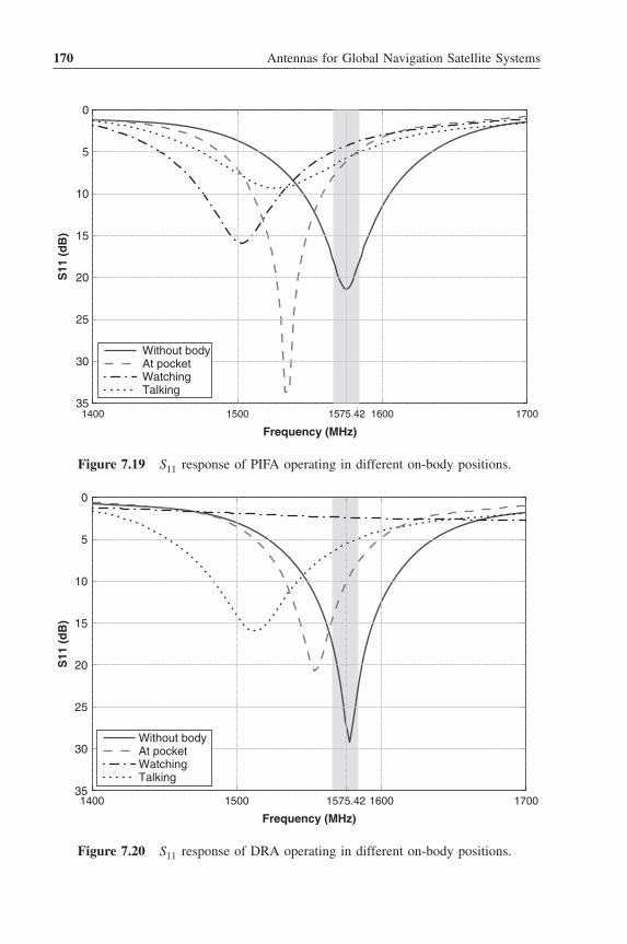
170 Antennas for Global Navigation Satellite Systems
1400 1500 1575.42 1600 170035
30
25
20
15
10
5
0
Frequency (MHz)
S11
(d
B)
Without bodyAt pocketWatchingTalking
Figure 7.19 S11 response of PIFA operating in different on-body positions.
1400 1500 1575.42 1600 170035
30
25
20
15
10
5
0
Frequency (MHz)
S11
(d
B)
Without bodyAt pocketWatchingTalking
Figure 7.20 S11 response of DRA operating in different on-body positions.
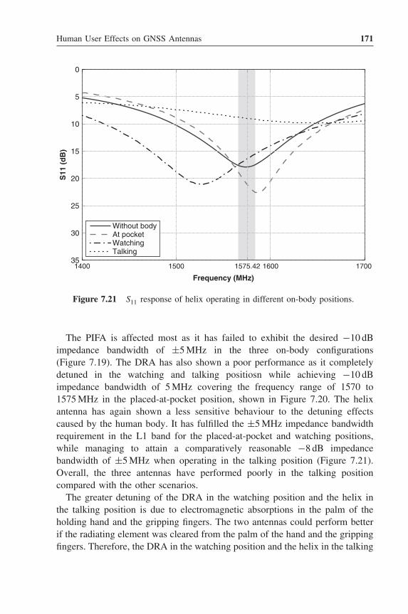
Human User Effects on GNSS Antennas 171
1400 1500 1575.42 1600 170035
30
25
20
15
10
5
0
Frequency (MHz)
S11
(d
B)
Without bodyAt pocketWatchingTalking
Figure 7.21 S11 response of helix operating in different on-body positions.
The PIFA is affected most as it has failed to exhibit the desired −10 dBimpedance bandwidth of ±5 MHz in the three on-body configurations(Figure 7.19). The DRA has also shown a poor performance as it completelydetuned in the watching and talking positiosn while achieving −10 dBimpedance bandwidth of 5 MHz covering the frequency range of 1570 to1575 MHz in the placed-at-pocket position, shown in Figure 7.20. The helixantenna has again shown a less sensitive behaviour to the detuning effectscaused by the human body. It has fulfilled the ±5 MHz impedance bandwidthrequirement in the L1 band for the placed-at-pocket and watching positions,while managing to attain a comparatively reasonable −8 dB impedancebandwidth of ±5 MHz when operating in the talking position (Figure 7.21).Overall, the three antennas have performed poorly in the talking positioncompared with the other scenarios.
The greater detuning of the DRA in the watching position and the helix inthe talking position is due to electromagnetic absorptions in the palm of theholding hand and the gripping fingers. The two antennas could perform betterif the radiating element was cleared from the palm of the hand and the grippingfingers. Therefore, the DRA in the watching position and the helix in the talking

172 Antennas for Global Navigation Satellite Systems
(a) (b)
Figure 7.22 Modified watching position for GPS mobile terminal DRA to investigateS11 response: (a) Original watching position; (b) Modified watching position (dz =40 mm).
(a) (b)
Figure 7.23 Modified talking position for GPS mobile terminal helix to investigateS11 response: (a) Original talking position; (b) Modified talking position (dz = 40 mm).
position are tested by moving the antenna 40 mm in the z-direction (dz). Thetwo tested configurations are shown in Figures 7.22b and 7.23b in comparisonwith the original positions (Figures 7.22a and 7.23a).
The S11 responses of the DRA and helix in the modified watching and talkingscenarios are plotted in Figures 7.24 and 7.25, respectively. It can be observedfrom these results that the two antennas exhibit better impedance matchingwhen placed at dz = 40 mm compared with the original positions. It is thereforeevident that the way a user holds the antenna plays a vital role in defining theextent of antenna detuning.

Human User Effects on GNSS Antennas 173
1400 1500 1575.42 1600 1700−35
−30
−25
−20
−15
−10
−5
0
Frequency (MHz)
S11
(d
B)
Free SpaceWatching: original positionWatching: dz=40 mm
Figure 7.24 Comparison of S11 curves for DRA in original and modified watchingpositions.
1400 1500 1575.42 1600 1700−35
−30
−25
−20
−15
−10
−5
0
Frequency (MHz)
S11
(d
B)
Free SpaceTalking: original positionTalking: dz=40 mm
Figure 7.25 Comparison of S11 curves for helix in original and modified talkingpositions.

174 Antennas for Global Navigation Satellite Systems
X
Z
Y
−17 dB
6 0 3−34
(i) PIFA (ii) DRA (iii) Helix
(a)
(i) PIFA (ii) DRA (iii) Helix
(b)
Figure 7.26 Simulated 3D gain patterns for perpendicular and parallel polarisationsof PIFA, DRA and helix GPS mobile terminal antennas placed at user’s pocket positionto evaluate effects of body presence on performance of GPS antennas: (a) G⊥; (b) G‖.
The 3D simulated gain patterns of the three antennas in different on-bodypositions are also observed and recorded, and depicted in Figures 7.26–7.28.The proposed statistical model for the GPS multipath environment is used forthe evaluation and comparison of the performance of the antennas in the threeon-body configurations. The realised gain is used in the calculations of ηc andMEGGPS to incorporate both the power absorption and detuning effects causedby the human body. Table 7.3 summarises these results in comparison withthe values observed when the antennas operate without the presence of thehuman body.
Figure 7.29 compares ηc and MEGGPS for the three antennas. These resultsfurther strengthen the fact that GPS mobile terminal antennas in the multipathenvironment undergo performance degradations due to the presence of the lossy

Human User Effects on GNSS Antennas 175
X
Z
Y
−17 dB
60 3−34
(i) PIFA (ii) DRA (iii) Helix
(a)
(i) PIFA (ii) DRA (iii) Helix
(b)
Figure 7.27 Simulated 3D gain patterns for perpendicular and parallel polarisationsof PIFA, DRA and helix GPS mobile terminal antennas held in user’s hand at watchingposition to evaluate effects of body presence on GPS antennas’ operation: (a) G⊥;(b) G‖.
human body. The operation of the three antennas depends upon the factorsdiscussed in the previous section, including clear sky view, shielding bodymass and antenna placement.
Human body presence causes a minimum drop of 3% in the GPS antenna’sηc and 1.5 dB in MEGGPS. The three antennas perform reasonably well in theplaced-at-pocket position. A greater clear view of the sky and enhanced gainlevels in directions away from the body, due to reflections from the surfaceof the body, act to minimise the degradations caused by the presence of thehuman body. The DRA antenna has shown the best performance because ofstronger radiation in the upper hemisphere with an ηc of 58% and MEGGPSof −7.2 dB. In the watching position, a larger gap between the torso and the

176 Antennas for Global Navigation Satellite Systems
X
Z
Y
−17 dB
6 0 3 −34
(i) PIFA (ii) DRA (iii) Helix
(a)
(i) PIFA (ii) DRA (iii) Helix
(b)
Figure 7.28 Simulated 3D gain patterns for perpendicular and parallel polarisations ofPIFA, DRA and helix GPS mobile terminal antennas held in user’s hand beside head intalking position for the evaluation of GPS antenna performance near the human body:(a) G⊥; (b) G‖.
antenna has reduced the tissue losses. The presence of the holding hand hasproved the major source of degradation in this case. The PIFA and helix antennahave exhibited an improved ηc of 69% and 85%, respectively, as a combinedresult of a less shielded radiating element and increased gain in the upperhemisphere because of the reflections from the palm and arm. However, thisincreased coverage is made less effective by a reduced MEGGPS of −13.2 dBand −8.0 dB, respectively, due to pattern deformations. On the other hand,the performance of the DRA has suffered greatly since the radiating elementis blocked to a larger extent by the palm and gripping fingers of the holdinghand. It has reduced its ηc to just 3% and MEGGPS to −24.8 dB.
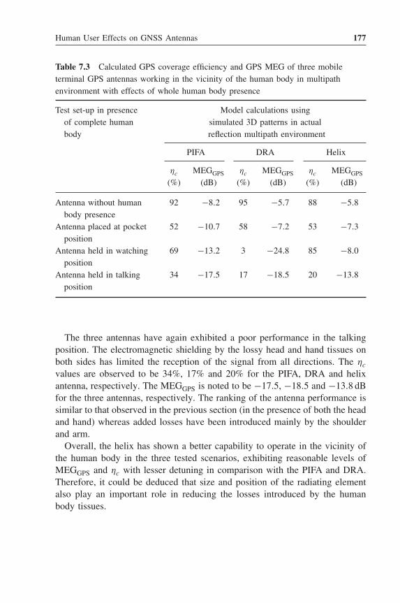
Human User Effects on GNSS Antennas 177
Table 7.3 Calculated GPS coverage efficiency and GPS MEG of three mobileterminal GPS antennas working in the vicinity of the human body in multipathenvironment with effects of whole human body presence
Test set-up in presence Model calculations usingof complete human simulated 3D patterns in actualbody reflection multipath environment
PIFA DRA Helix
ηc MEGGPS ηc MEGGPS ηc MEGGPS
(%) (dB) (%) (dB) (%) (dB)
Antenna without humanbody presence
92 −8.2 95 −5.7 88 −5.8
Antenna placed at pocketposition
52 −10.7 58 −7.2 53 −7.3
Antenna held in watchingposition
69 −13.2 3 −24.8 85 −8.0
Antenna held in talkingposition
34 −17.5 17 −18.5 20 −13.8
The three antennas have again exhibited a poor performance in the talkingposition. The electromagnetic shielding by the lossy head and hand tissues onboth sides has limited the reception of the signal from all directions. The ηc
values are observed to be 34%, 17% and 20% for the PIFA, DRA and helixantenna, respectively. The MEGGPS is noted to be −17.5, −18.5 and −13.8 dBfor the three antennas, respectively. The ranking of the antenna performance issimilar to that observed in the previous section (in the presence of both the headand hand) whereas added losses have been introduced mainly by the shoulderand arm.
Overall, the helix has shown a better capability to operate in the vicinity ofthe human body in the three tested scenarios, exhibiting reasonable levels ofMEGGPS and ηc with lesser detuning in comparison with the PIFA and DRA.Therefore, it could be deduced that size and position of the radiating elementalso play an important role in reducing the losses introduced by the humanbody tissues.
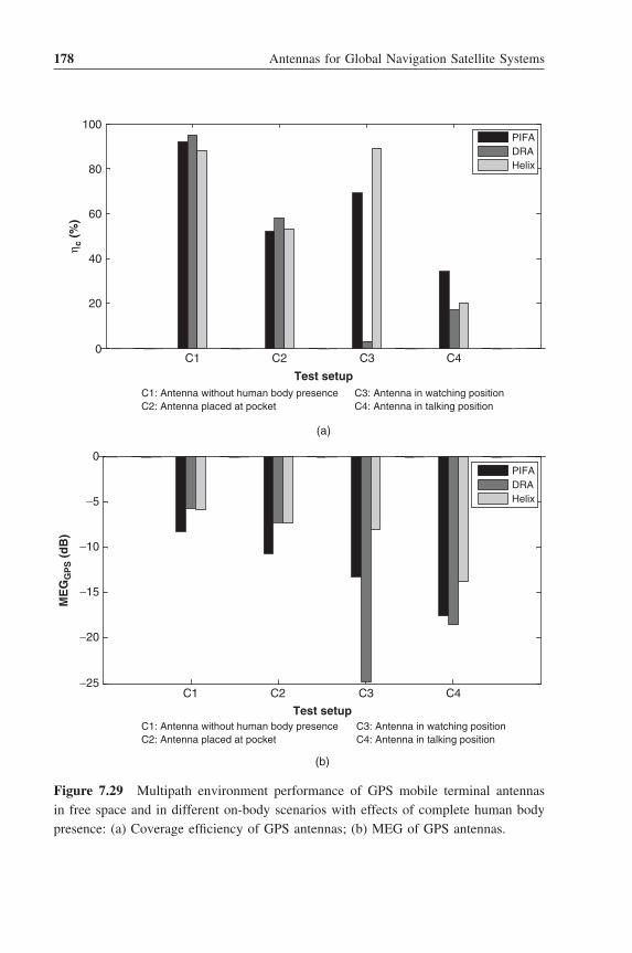
178 Antennas for Global Navigation Satellite Systems
C1 C2 C3 C40
20
40
60
80
100
Test setup
η c (
%)
PIFADRAHelix
(a)
C1 C2 C3 C4−25
−20
−15
−10
−5
0
Test setup
ME
GG
PS (
dB
)
PIFADRAHelix
(b)
C1: Antenna without human body presenceC2: Antenna placed at pocket
C3: Antenna in watching positionC4: Antenna in talking position
C1: Antenna without human body presenceC2: Antenna placed at pocket
C3: Antenna in watching positionC4: Antenna in talking position
Figure 7.29 Multipath environment performance of GPS mobile terminal antennasin free space and in different on-body scenarios with effects of complete human bodypresence: (a) Coverage efficiency of GPS antennas; (b) MEG of GPS antennas.

Human User Effects on GNSS Antennas 179
References1. Jensen, M.A. and Rahmat-Samii, Y. ‘EM interaction of handset antennas and human in
personal communications’, IEEE Transactions on Antennas and Propagation , 83, 7–17, 1995.2. Toftgard, J. Hornsleth, S. and Anderson, J.B. ‘Effects on portable antennas of the presence
of a person’, IEEE Transactions on Antennas and Propagation , 41, 739–746, 1993.3. Okoniewski, M. and Stuchly, M.A. ‘A study of the handset antenna and human body inter-
action’, IEEE Transactions on Microwave Theory and Techniques , 44, 1855–1864, 1996.4. Mason, P.A. Hurt, W.D. Walters, T.J. et al. ‘Effects of frequency, permittivity and voxel size
on predicted specific absorption rate values in biological tissue during electromagnetic fieldexposure’, IEEE Transactions on Microwave Theory and Techniques , 48, 2050–2058, 2000.
5. Hall, P.S. and Hao, Y. Antennas and propagation for body-centric wireless networks , ArtechHouse, London, 2006.
6. Wang, J. and Fujiwara, O. ‘EM interaction between a 5GHz band antenna mounted PC anda realistic human body model’, IEICE Transactions on Communications , E88-B, 2604–260,2005.
7. G.A. Conway and W.G. Scanlon, ‘Antennas for over-body-surface communication at2.45 GHz’, Transactions on Antennas and Propagation , 57, 844–855, 2009.
8. M. Sanad, ‘Effect of the human body on microstrip antennas’, IEEE Antennas and PropagationSociety International Symposium (AP-S), Vol. 1, pp. 298–301, June 1994.
9. H.R. Chuang, ‘Human operator coupling effects on radiation characteristics of a portable com-munication dipole antenna’, IEEE Transactions on Antennas and Propagation , 42, 556–560,1994.
10. Colburn, J.S. and Rahmat-Samii, Y. ‘Human proximity effects on circular polarized handsetantennas in personal satellite communications’, IEEE Transactions on Antennas and Propa-gation , 46, 813–820, 1998.
11. CENELEC, European Specification, ‘Considerations for the evaluation of human exposureto electromagnetic fields (EMFs) from mobile telecommunication equipment (MTE) in thefrequency range from 30 MHz-6 GHz’, ES-59005:1998 E, 1998.
12. Ur Rehman, M. Gao, Y. Chen, X. and Parini, C.G. ‘Effects of human body interferenceon the performance of a GPS antenna’, European Conference on Antennas and Propagation(EuCap), November 2007.
13. Ur Rehman, M. Gao, Y. Chen, X. Parini, C.G. and Ying, Z. ‘Mobile terminal GPS antennasin multipath environment and effects of human body presence’, Loughborough Antennas andPropagation Conference (LAPC), November 2009.
14. Ur Rehman, M. Gao, Y. Chen, X. Parini, C.G. and Ying, Z. ‘Impacts of human body onbuilt-in GPS antennas for mobile terminal in multipath environment’, European Conferenceon Antennas and Propagation (EuCap), April 2010.
15. Federal Communication Commision, ‘FCC’s wireless 911 rules’, http://www.fcc.gov/guides/wireless-911-services (accessed 25 September 2011)
16. Nielsen, J.O. and Pedersen, G.F. ‘Mobile handset performance evaluation using radiationpattern measurements’, IEEE Transactions on Antennas and Propagation , 54, 2154–2165,2006.
17. Krogerus, J. Ichelun, C. and Vainikainen, P. ‘Dependence of mean effective gain of mobileterminal antennas on side of head’, European Conference on Wireless Technology (ECWT),pp. 467–470, October 2005.

180 Antennas for Global Navigation Satellite Systems
18. Douglas, M.G. Okoniewski, M. and Stuchly, M.A. ‘A planar diversity antenna for handheldPCS devices’, IEEE Transactions on Vehicular Technology , 47, 747–754, 1998.
19. Fujimoto, K. and James, J.R. ‘Mobile antenna systems handbook ,’ 2nd edn, Artech House,Boston, MA, 2001.
20. Pedersen, G.F. and Andersen, J.B. ‘Handset antennas for mobile communications: integration,diversity, and performance,’ Radio Science Review Oxford University Press, Oxford, 1999.
21. Ogawa, K. and Uwanao, T. ‘Mean effective gain analysis of a diversity antenna for portabletelephones in mobile communication environments,’ Electronics and Communication in Japan(Part I: Communications), 83, 88–96, 2000.
22. CST Microwave Studio R©, 2010 User Manual.23. Balanis, C. Antenna theory analysis and design , 2nd edn, John Wiley & Sons, Inc.,
New York, 1997.24. Gabriel, C. ‘Compilation of the dielectric properties of body tissues at RF and microwave
frequencies’, Brooks Air Force Technical Report, AL/OE-TR-1996-0037 , 1996.25. ‘Calculation of the dielectric properties of body tissues,’ Institute of Applied Physics, Italian
National Research Council, http://niremf.ifac.cnr.it/tissprop (accessed 1 November 2011).26. Federal Communication Commision, ‘Body tissue dielectric properties,’ /www.fcc.gov/oet/
rfsafety/dielectric.html (accessed 2 November 2011).27. Jemai, J. Kurner, T. Varone, A. and Wagen, J.F. ‘Determination of the permittivity of build-
ing materials through WLAN measurements at 2.4 GHz’, IEEE International Symposium onPersonal, Indoor and Mobile Radio Communications, September 2005.
28. Klysza, G. Balayssaca, J.P. and Ferriresb, X. ‘Evaluation of dielectric properties of con-crete by a numerical FDTD model of a GPR coupled antenna parametric study’, NDT & EInternational , 41, 621–631, 2008.
29. Ur Rehman, M. Gao, Y. Alfadhl, Y. et al . ‘Study of human body exposure to RF sig-nal at UHF frequencies,’ Joint Meeting of Bioelectromagnetics Society and the EuropeanBioelectromagnetics Association (BioEM), June 2009.
30. Ur Rehman, M. Gao, Y. Wang, Z. et al ‘Investigation of on-body Bluetooth transmission,’IET Microwaves, Antennas and Propagation , 4, 871–880, 2010.

8Mobile Terminal GNSSAntennas
8.1 Introduction
This chapter deals with the limitations of antenna size and shape that areimposed when GNSS functions are to be added to small devices such as mobilehandsets and personnel trackers. It is shown how the radiation patterns andpolarisation properties of the antenna can be radically changed by factors suchas the positioning of the antenna on the platform. The presence of a highlysensitive receiver system imposes severe constraints on the permitted levels ofnoise that may be generated by other devices on the platform without impair-ing the sensitivity of the GPS receiver; the chapter will describe the designprecautions that must be taken to reduce these to an acceptable level. The casestudies provide measured results from real applications, illustrating a numberof typical performance defects and indicating possible solutions.
The essential properties of an antenna for a GNSS receiver are that it hasa radiation pattern that covers as much of the sky as possible with the userdevice in its normal operating position, and that it has as high a gain, for anRHCP signal, as is consistent with the wide pattern beamwidth.
Almost all low-cost mobile terminals use only the L1 signal from the GNSSsatellites. This has the advantage that the antenna can operate in only onefrequency band, although to cover all the available and near-future systems,the L1 signal frequencies differ between systems as shown in Table 1.1.
Antennas for Global Navigation Satellite Systems, First Edition.Xiaodong Chen, Clive G. Parini, Brian Collins, Yuan Yao and Masood Ur Rehman.© 2012 John Wiley & Sons, Ltd. Published 2012 by John Wiley & Sons, Ltd.

182 Antennas for Global Navigation Satellite Systems
The last few years have seen a huge upsurge in the number and varietyof consumer equipment making use of GNSS-derived location data. In manyconsumer platforms, for example mobile phone handsets and cameras, there isinadequate space for a conventional GNSS antenna, and the physical orientationof the platform when in use may make it difficult to provide an antenna witha clear view of the sky. Fortunately there is substantial latitude in the antennarequirement and a variety of solutions has been used successfully.
Mobile user equipments (UEs) present several problems in their use of GNSSservices. A UE will frequently be used at locations in which the device hasa limited view of the sky. A user standing immediately outside an isolatedbuilding will have a view of only one-half of the sky. This immediately halvesthe number of satellites that are potentially visible, perhaps from 10 to 5, whichis likely to result in a fix with lower precision than would have been expectedunder open sky conditions. Thus:
• The total amount of positional information is halved – there are fewer inde-pendent estimates of position which can be used to produce the positioninformation received by the user.
• The geometry of the available satellites is likely to result in a larger dilutionof precision than would have been possible with a view of the whole sky.
• The strongest signals may be lost because the satellites that would haveprovided them are shielded from view by the building.
In a city street among high buildings the chance of a fast and accurate fix isfurther reduced. The number of satellites in view falls because only a smallstrip of sky is visible, most of the visible satellites are roughly in line withthe direction of the street, so the fix will have poor precision in the transversedirection, and signals from satellites that are not directly visible will be receivedvia reflections – perhaps multiple reflections – from the surrounding buildings.
A mobile UE has the additional penalties of lack of physical space in whichto accommodate antennas (it often has to use small antennas) and of limitedbattery life (it may have reduced possibilities to maintain or refresh positionalinformation while the device is not in use). A further design issue is the poten-tially close physical spacing between the GNSS antennas and other antennasand associated electronic devices on the platform, such as processors, camerasand memory. As well as the obvious possibilities of interference from strongtransmitted signals, many of these devices produce broadband noise at levelswhich may exceed that of the signals received from distant satellites.
It will be seen from this short summary that the use of GNSSs on smalluser platforms presents a number of challenges, many of which are beyond

Mobile Terminal GNSS Antennas 183
the control of the antenna designer. However, when a proven GNSS receiveris fitted to a new mobile device and the time to first fix is long, the carrier-to-noise ratio of the visible satellites is low, or the resulting position data isless accurate than expected, the problem is often taken to the antenna designerwho is expected to be able to provide a solution. It is therefore important forantenna engineers to know something of the operation of the whole GNSS, andalso for system-level device designers to understand the issues that relate toantenna design and placement on the platform.
8.2 Antenna Specification Parameters
We now review the specification parameters for any GPS antenna, and considertheir impact on system performance.
8.2.1 Polarisation
GNSS satellites radiate RHCP signals, so an ideal user terminal will be providedwith an RHCP antenna. Reflected signals will have reached the receiver with alonger flight time than direct signals, so any calculations made from them willbe inaccurate. After a single reflection, signals will have left hand polarisation,so they can be suppressed by ensuring that the antenna will respond only toRHCP signals. The ground is a potent source of reflected signals, but to rejectground-reflected signals from satellites at low elevation angles the antennaneeds a high axial ratio at these angles. Unfortunately, the polarisation radiatedby most RHCP antennas in the rear hemisphere is LHCP, so the only way toreject ground reflections is by ensuring a high rate of roll-off of sensitivity atelevation angles below 10◦ or so from the horizon.
A real UE will often be used in city streets in which there may be multiplereflections, many of which will have RHCP. As with many other characteristicsof the antenna (radiation pattern, gain and impedance), its polarisation dependsheavily on the interaction between the antenna and the platform on whichit is mounted. Any unbalanced (single-terminal) antenna operates because itcreates currents in the groundplane of the platform; these groundplane currentsradiate, so their directions and phases, together with the direct radiation fromthe antenna, determine the polarisation of the whole device. To complicatematters further, the effective polarisation will vary substantially with satellitedirection and the orientation of the platform.
As a result of all these factors, the difference in performance of antennaswith differing polarisations is less than might be expected, and it is commonto find antennas with both nominal RHCP and nominal linear polarisation in

184 Antennas for Global Navigation Satellite Systems
use with apparently equal success. A linearly polarised antenna occupies lessarea than a patch and is likely to be less loaded; if so it may outperform thesmaller patches [1].
It seems reasonable that antenna/platform assemblies are compared by mea-suring their performance when illuminated by an RHCP signal, and the resultsshown in this chapter adhere to this convention except where explicitly statedotherwise. In the same way, all references to the shape and direction of radiationpatterns relate to the RHCP component.
8.2.2 Radiation Patterns
The radiation pattern of a GNSS antenna should cover as much of the sky aspossible when the platform is in its use position. The use position of differentplatforms may be substantially different – for example, typical in-car PNDs aremounted with the display almost vertical, while a smartphone or other handhelddevice will often be used with the screen uppermost. A device intended forvehicle location may be mounted in a concealed position with a very limitedview of the sky and in close proximity to metal surfaces, while a handhelddevice may interact strongly with the user’s body.
In general, the ideal radiation pattern for a GNSS antenna is an upward-looking hemisphere, providing gain to all satellites that are visible in the sky.An antenna with too small a beamwidth may have a correspondingly highergain, but provided that the received signal is adequate to provide a carrier-to-noise (C/N0) ratio in excess of around 35 dB, a more accurate fix is providedby acquiring more satellites rather than simply increasing the signal from thosesatellites lying within a limited effective antenna beamwidth.
8.2.2.1 Radiation Pattern Measurement
Passive radiation patterns are measured using standard techniques, illuminatingthe device under test (DUT) with an RHCP antenna fed by a signal sourcein the usual way. Using a measuring receiver we can plot the gain of theantenna/platform combination in two or three dimensions, depending on thecapabilities of the measurement range. These measurements will allow us tooptimise the position of the antenna on the platform and measure RHCP gainand efficiency. Measurements of this kind are usually made at the beginningof the development cycle for a new UE and they provide an indication of thegeneral level of performance that can be anticipated from the proposed device if

Mobile Terminal GNSS Antennas 185
other design aspects are well managed. In particular, they will serve to confirmthat the polarisation and radiation patterns are suitable.
A better indication of the performance of a working platform is providedby illuminating the DUT by means of a satellite simulator, and equipping theDUT with an on-board operational GNSS receiver. The C/N0 ratio recordedby the receiver is then plotted as a function of bearing of the signal source fromthe platform. To avoid the enhancement of the signal which may be caused bythe connection of a cable to a very small UE, the output from the receiver maybe transmitted by radio (including GPRS, Wi-Fi or Bluetooth), by an opticalfibre, or by a carefully decoupled and isolated data cable.
If this measurement is carried out on a fully working UE, the result includesany interference produced on the UE platform. We can compare the measuredC/N0 performance with what we expect, given the measured antenna gain andknown receiver noise figure. If these fail to match, we can then seek the cause,which is likely to be radiated or conducted noise, spurious emissions from otherdevices, or blocking from other transmitters on the platform. While these arenot ‘antenna problems’, it is usually the antenna engineer who has the test gearand expertise to investigate and cure them.
Electromagnetic compatibility (EMC) issues on small mobile platforms, withclosely integrated antennas, are more likely than with separate ‘active’ antennas(with an associated low-noise amplifier (LNA)), simply because the separateantenna is not subject to the noise environment on the platform and the increasein signal level provided by the LNA reduces the relative level of on-platforminterference. In general, this is not a function of the type of antenna used, butis caused by the proximity of the antenna and the intrinsically higher level ofinteraction when the antenna is mounted directly on the platform.
8.2.3 Impedance
In general we require the antenna to provide a close match to 50 �. In thecase of a UE provided with a radio transmitter – for the cellular communi-cations bands, Wi-Fi, Bluetooth or other interfaces – the receiver is likely tobe preceded by a bandpass SAW filter, so the possibility of employing noise-matching rather than power-matching at the receiver input is limited. Whilealmost all compact GNSS antennas have an unbalanced output, some receiverchips have a balanced (differential) input, so a balun network or chip compo-nent may be needed between the antenna and the receiver – some SAW filtersprovide a single-ended input and balanced output for this application. The input

186 Antennas for Global Navigation Satellite Systems
impedance of a SAW filter may be mismatched from 50 � and some improve-ment in performance may be provided by providing an input matching networkbetween the antenna and the filter. The provision for a matching network alsoallows for the compensation of the effects of the platform – including that ofthe plastic case – on the impedance of the antenna.
An antenna requires only a very small fractional bandwidth to cover theL1 frequency band, but the tendency of platform designers to demand ever-smaller antennas has led to the progressive reduction of patch antennas fromthe original 25 × 25 mm2 to as little as 12 × 12 mm2. This reduces the availablebandwidth and many antenna designs rely on individual tuning by trimmingits dimensions – a process often carried out using a laser. Some of these smallantennas are easily detuned by surrounding objects or by the presence of theuser. Other antenna designs that are heavily loaded to reduce their dimensionsmay suffer the same problem. Mismatch reduces the effective sensitivity of thereceiver and is therefore to be avoided.
The VSWR of an internal antenna is only significant in its impact on signaltransfer to the receiver. Optimising the impedance of the antenna is part ofthe optimisation of its efficiency; the ‘best’ impedance is whatever providesthe highest sensitivity and delivers the highest C/N0 ratio in a given signalenvironment.
If an external antenna is used, its VSWR is important because any significantdeviation from 50 � may result in critical dependence on the exact electricallength of the interconnecting coaxial cable – something which the user mayadjust, for example to suit the fit in a vehicle. For this reason the VSWRshould typically be less than 2:1.
8.2.4 Gain/Efficiency
Given the very low signal strength available from the GNSS satellites, it is clearthat we should obtain as much gain from the antenna as possible. Unfortunatelythe requirement that the antenna must have an approximately hemisphericalradiation pattern restricts the directivity, and hence the gain, we can realise.If the antenna were lossless and we could obtain an efficiency of 100%, itsgain would be 3 dBic; with a more realistic efficiency we would do well toachieve a mean gain over a hemisphere of 1 dBic. We can degrade this, bypoor polarisation matching or poor design of the antenna or the platform, butwe can do little to increase it.
The only option open to us to increase the sensitivity of the receiver is toensure that its noise figure is a small as possible. If the receiver already hasa very low noise figure – less than say 1.2 dB – we must avoid degrading it

Mobile Terminal GNSS Antennas 187
by introducing loss between the antenna and the receiver. If the noise figure ishigher than this we should consider preceding the input to the receiver with anLNA – typically with a gain of 16–20 dB and a noise figure less than 1 dB. Ifthe UE has provision for the optional use of an external antenna connected bya coaxial cable, this antenna would usually incorporate an LNA – a so-calledactive antenna . Introducing too much front-end gain in an effort to reduce thenoise figure is not good practice – the resulting C/N0 reported by the receivermay look impressively low, but the dynamic range of the system may beseverely reduced and susceptibility to blocking correspondingly increased.
8.2.5 Weight
In today’s compact, but highly complex consumer electronics, weight is asignificant issue, and every opportunity is taken by designers to reduce theweight of every component. Even an antenna that weighs 2 g is too heavy ifthe same result could have been obtained from one weighing only 1 g!
8.2.6 Bandwidth
In the earlier chapters of this book we have described a wide variety of antennasthat are suitable for use with GPS receivers. For some GPS applications thefirst priority is to obtain position or navigation data which has the highestpossible accuracy. Such applications include surveying and aircraft navigation.To achieve high accuracy, the most obvious steps are to compensate for theerrors created by the propagation medium and to reduce the extent to whichreflected signals can enter the receiver. A further major increase in accuracymay be obtained by using the phase of the signals received from the satellitesfor the calculation of position. All these have requirements in terms of theperformance of the antenna.
Compensation of ionospheric propagation delays requires that we receivesignals at more than one frequency. These will typically be the L1 and L2signals at approximately 1575 MHz and 1227 MHz. The delay caused by iono-spheric effects is a function of the transmission frequency and of the elevationand direction of the path from each satellite. By receiving signals from eachsatellite at two well-spaced frequencies it is possible to compute the excessdelay caused on each path, reducing the potential uncertainty in the estimatedposition of the receiver. In order to do this, we need a dual-frequency antenna.
In practice, although the uncertainties of propagation give rise to the largestcontribution to clear sky error in a modern GPS system, at the time of writingmost portable devices use only the L1 signal.

188 Antennas for Global Navigation Satellite Systems
8.2.7 Phase Performance
Use of the phase of the received signal to refine the position estimate requiresthat, to the extent possible, it should not be a function of its angle of arrivalrelative to the antenna. For surveying, precision navigation and other applica-tions requiring high position accuracy, perhaps down to a few centimetres, wemust do whatever is necessary to achieve high accuracy. This requires the useof antennas which are designed to maintain stable phase characteristics andwhich can be used in an environment free from user influences. The objectiveof a completely stable and well-defined phase centre in both azimuth and ele-vation planes, and whose position is independent of frequency, is not reallyachievable, so a compromise is reached by applying measured calibration datato compensate the remaining variability in phase as a function of the directionof each satellite. This further implies that we know both the compass bearingand attitude of the antenna in order to apply these corrections accurately. Forsurveying applications the GPS antenna will be supported by a device similarto a theodolite, while for navigational purposes these additional variables maybe obtained from independent sensors.
8.3 Classification of GNSS Terminals
8.3.1 Geodetic Terminals
These are the most accurate GNSS terminals and are typically found infixed-site GNSS applications. Their antennas cover multiple frequencybands to enable compensation of propagation effects, and will increasinglyprovide reception of satellites for multiple GNSSs. This will providehigher reliability – resistance to ground sector failures and not just satellitefailures – and greater accuracy, especially in situations with a restricted viewof the sky. They are usually fitted with choke-ring antennas which provide therequired radiation pattern performance but are relatively costly, large and heavy.
8.3.2 Rover Terminals
These are typically used in land survey, forestry, construction, and otherportable or mobile applications. They provide the user with good accuracywhile being optimised for portability. The antenna for a rover terminal istypically mounted on a handheld pole and fires vertically upwards. Thiscontrols the attitude of the antenna within reasonably narrow limits, although

Mobile Terminal GNSS Antennas 189
the azimuth orientation of the antenna may be uncontrolled. The position andhigh front-to-back ratio of the antenna assist by reducing operator-reflectionmultipath and ground noise pickup. These antennas are designed to providerapid roll-off at low elevation angles to reduce multipath and the maintenanceof a low axial ratio to maximise receive signal gain and reduce phase centrevariations as far as possible. Their size, weight, performance and cost arepractical compromises based on the application to be served.
8.3.3 General Purpose Mobile Terminals
These provide sufficient accuracy for consumer applications such as in-carnavigation, personnel trackers, geo-tagging of photographs and social media.They also serve a wide range of commercial applications such as the tracking ofgoods and vehicles, and the location of handheld payment and receipt terminals.These terminals use a variety of antenna types, mainly determined by their lowcost and small occupied volume. Fortunately, for these applications a medianerror (CEP) of between 2 and 3 metres is acceptable and it can be achieved bymodern GPS receivers using s single frequency and a simple low-cost antenna.It is important to understand that the use of these antennas on small consumerplatforms represents a large compromise in potential performance, but for manypurposes the convenience and low cost of these devices outweigh their limitedaccuracy.
Table 8.1 gives a summary of the general classification of GNSS mobileterminals.
Table 8.1 General classification of GNSS terminals
Geodetic Rover Handheld
Frequency bands Multiple Single/multiple Single, L1Radiation patterns Tightly optimised Controlled UncontrolledPhase behaviour Characterised and
compensated in 3DModerate, not
compensatedNot relied upon
Multipath suppression Excellent Good NoneDimensions Large Medium Small/very smallWeight Heavy Portable Almost noneCost High Medium Very low

190 Antennas for Global Navigation Satellite Systems
Three additional constraints are important in many of the applications whichwe will consider in this chapter, as follows.
8.3.3.1 Sensitivity
For smartphones, personnel trackers and many other applications it is desirablethat GNSS position should be available even in poor signal conditions – withlimited sky view, or perhaps even no direct satellite view. It is also verydesirable that position is reacquired as soon as possible when the device movesfrom a shadowed position into an area with better signal coverage.
• Time to first fix (TTFF): It is important for many applications that position isacquired rapidly on start-up. Lack of sensitivity will result in slow acquisitionof satellites on start-up, especially when the device has a partial view ofthe sky.
• Battery drain: All portable devices are limited by the capacity of their bat-teries. Most GNSS receivers have a variety of low-power ‘sleep’ modesavailable, in which they maintain only minimal memory contents and wakefrom time to time to refresh their clock offsets and ephemeris data. Theseactivities require substantial battery current, so if they are prolonged by lackof signal the effective battery life will be substantially reduced.
8.4 Antenna Designs for Portable User Equipment
8.4.1 Short Quadrifilar Helices
Early antennas for UEs were usually in the form of short helices. Thesebecame popular after the introduction of dielectrically loaded resonant quadri-filar helices, and this form of antenna has proved remarkably durable. Its maindrawbacks are a form factor which is not always easy to accommodate in asmall, tightly packed UE, and a relatively high price by current standards. Theseantennas are typically only 12 mm high at 1575 MHz (0.063λ) but suffer theconsequent penalties of low radiation resistance, high Q-factor and the need fortight production tolerances. The characteristic shape and size of their upward-projecting outline are still typical of many user devices. A quadrifilar helix hasthe advantage of being a balanced antenna, and when suitably dimensioned itsradiation pattern can provide high efficiency for RHCP reception and a radi-ation pattern covering a wide arc of the sky. Being balanced, the antenna ismuch less dependent on currents generated in the device on which it is placedthan is the case with an unbalanced antenna. As described in [2] and illustrated

Mobile Terminal GNSS Antennas 191
Fish-hook feed
Radiating section
Sleeve balun withcrowned rim
Figure 8.1 Short backfire quad-helix [2]. Reproduced with permission from IET.
in Figure 8.1, the antenna is realised as a copper track etched or deposited on ahigh-K dielectric core. An integral balun is formed as a short-circuit λ/4 coaxialsleeve, much shortened by the presence of the dielectric inside it. The antennacomprises two bifilar helical loops. One is adjusted to be slightly longer thanresonant length to produce an input impedance with a phase angle of +45◦,and the other bifilar is adjusted to be shorter than resonance to produce aninput impedance with a phase angle of +45◦. This produces the required 90◦
phase shift between the currents in the first bifilar winding with respect to thesecond bifilar winding.
The penalty for the substantial size reduction achieved by this very success-ful design is the low feed impedance (R = 2 �) and the consequent narrowbandwidth over which it can be matched to 50 �.
This antenna provides a radiation pattern with a large beamwidth, alignedwith the axis of the structure and directed away from the grounded end of theelements. In order to face the sky, this type of antenna is mounted on the upperedge of the host platform.
8.4.2 Patch Antennas
An alternative early form of small GNSS antenna was a square patch. Whenconstructed using a suitable dielectric material between the substrate and theradiating patch, this is around 25 mm square, and with an off-centre feed and/ora truncated corner it can provide the desired circular polarisation. A patchcreates a radiation pattern directed orthogonally away from the surface onwhich it is mounted. This is no problem if the surface is horizontal – like theroof of a car – but became a problem when integral antennas were neededfor satellite navigation devices to be used inside cars. In this application thescreen is oriented towards the driver and only the top of the package faces the
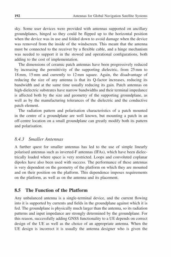
192 Antennas for Global Navigation Satellite Systems
sky. Some user devices were provided with antennas supported on ancillarygroundplanes, hinged so they could be flipped up to the horizontal positionwhen the device was in use and folded down to avoid damage when the devicewas removed from the inside of the windscreen. This meant that the antennamust be connected to the receiver by a flexible cable, and a hinge mechanismwas needed to support it in the stowed and operational configurations, bothadding to the cost of implementation.
The dimensions of ceramic patch antennas have been progressively reducedby increasing the permittivity of the supporting dielectric, from 25 mm to18 mm, 15 mm and currently to 12 mm square. Again, the disadvantage ofreducing the size of any antenna is that its Q-factor increases, reducing itsbandwidth and at the same time usually reducing its gain. Patch antennas onhigh-dielectric substrates have narrow bandwidths and their terminal impedanceis affected both by the size and geometry of the supporting groundplane, aswell as by the manufacturing tolerances of the dielectric and the conductivepatch element.
The radiation pattern and polarisation characteristics of a patch mountedin the centre of a groundplane are well known, but mounting a patch in anoff-centre location on a small groundplane can greatly modify both its patternand polarisation.
8.4.3 Smaller Antennas
A further quest for smaller antennas has led to the use of simple linearlypolarised antennas such as inverted-F antennas (IFAs), which have been dielec-trically loaded where space is very restricted. Loops and convoluted coplanardipoles have also been used with success. The performance of these antennasis very dependent on the geometry of the platform on which they are mountedand on their position on the platform. This dependence imposes requirementson the platform, as well as on the antenna and its placement.
8.5 The Function of the Platform
Any unbalanced antenna is a single-terminal device, and the current flowinginto it is supported by currents and fields in the groundplane against which it isfed. The groundplane is physically much larger than the antenna, so its radiationpatterns and input impedance are strongly determined by the groundplane. Forthis reason, successfully adding GNSS functionality to a UE depends on correctdesign of the UE as well as the choice of an appropriate antenna. When theUE design is incorrect it is usually the antenna designer who is given the

Mobile Terminal GNSS Antennas 193
task of finding out what has gone wrong, and then persuading others that theirdesign was inadequate to provide acceptable antenna performance. A muchmore satisfactory design method is to understand the way in which a successfulplatform is designed to provide the necessary RF performance. The effects to beconsidered are those on antenna efficiency (gain), noise environment, radiationpattern and polarisation.
8.5.1 Antenna Efficiency, Gain and Noise
A successful design requires that the host platform provides a continuousgroundplane, with at least one dimension preferably approximating a free spacehalf wavelength – this is around 65 mm. Ground currents will flow in the outer-most conducting layer on the platform, so to avoid received power disappearinginto DC feed lines, digital lines and other circuits, it is good practice to providean essentially continuous copper ground conductor on the face of the PCB sup-porting the antenna. To ensure the highest antenna gain, the groundplane shouldnot be interrupted by long tracks, especially those aligned at right angles tothe antenna-induced currents. It is perfectly acceptable to provide holes in thegroundplane so electronic components, fed from below, can be accommodatedon the board. An even better result will be obtained if we provide a continuouscopper layer on the other face of the PCB stack, and provide vias all aroundthe edge of the PCB to tie the two outer groundplanes together. Not only hasthis provided a clear path for RF currents on both sides of the platform, but atthe same time we have created a screened box, inside which lie all the noisylines connected to processors, memory, clocks, switch-mode power suppliesand other circuits which will raise the noise floor at the GNSS frequencies andreduce the ability of the receiver to see the very low-level signals arriving fromGNSS satellites. While laying out the PCB it is prudent to allow for screeningcans to be placed over all the chips supporting noisy functions. They may notbe needed if the separation between the antenna and the chip is sufficient andthe groundplane design is adequate, but if they are needed they can be addedwithout the necessity of a board respin.
The environment of a small mobile UE is often very challenging for GNSSuse, with co-sited transmitters and other electronic devices. The available iso-lation between small unbalanced antennas is often restricted by the presence ofcommon-mode ground currents and there is little physical room to provide spa-tial separation – on a typical platform the available isolation may be as smallas 12 dB. Fortunately, very high-Q bandpass SAW filters are available for theGNSS bands, and when cellular and GPS radios operate on the same platformit is general practice to fit SAW filters both preceding and following the LNA

194 Antennas for Global Navigation Satellite Systems
at the front of the receiver. These naturally create a small reduction in receivernoise performance, but they effectively prevent blocking of the LNA by strongout-of-band signals.
A more insidious problem arises if a cellular transmitter has a poor out-of-band noise performance. Noise within the GPS band cannot be filtered by usinga bandpass filter in front of the receiver, so the problem must be tackled byadding a notch filter in the transmitter output – or, better, by using a transmitterwith lower broadband noise levels.
8.6 Comparing Antenna Performance on UEs
8.6.1 Drive Testing
An engineer who has designed a GNSS antenna for a portable UE will fre-quently be expected to demonstrate its functionality by conducting a ‘drivetest’. One or more portable UEs are taken in a vehicle and driven around whilelogging such parameters as the position of the vehicle, the number and C/N0ratios of the satellites used to provide each fix, and perhaps the TTFFs forvarious starting conditions. A test of this kind clearly in some way representspotential user experience, but as a method for comparing antennas, receiversor software it must be used with caution, and with an understanding of all thefactors which can influence the performance of a GNSS receiver system.
One of the most important features of any test method must be that theresult can be repeated. Unfortunately the constantly changing configurationof the GNSS satellites in orbit and the movement of a vehicle through theenvironment – particularly that of a high-rise city – effectively create a uniqueevent. We cannot expect that carrying out the same test within an hour, oreven at the same time on a different day, will provide the same results. Theymay be similar, but there may be wide variations in some parameters. Theseare to be expected – the vehicle may be in different positions on the roadin subsequent tests and the satellite configuration will be different, causinglarge potential differences in the accuracy of position, especially in canyonstreets. Effects of other traffic will vary; the duration of halts in traffic or attraffic signals will vary; the duration of periods out of range of signals mayalso vary – for example, while shadowed by tall buildings or waiting underbridges. The duration of a cold-start TTFF is a function of the time of startrelative to the timing of data frames transmitted from the satellites; in urbanconditions, and especially when on the move, the TTFF may be extended byshadowing from trees, buildings and other traffic and may be expected to differwidely between different cold starts even with the same equipment.
Mobile Terminal GNSS Antennas 195
There are two methods by which this situation can be improved. Wherepossible, comparative trials should be conducted on two or more devices simul-taneously, so the environmental variables are as near as possible the same foreach; alternatively trials must be conducted a number of times and the resultsevaluated on a statistical basis.
There is always some conflict between the need to provide a user with someusable position information and the requirement for this to be accurate. Thisconflict has no unique solution, but the optimum for any user depends on theapplication. Many receivers provide configurable settings for parameters suchas the lowest elevation angle for a satellite that will be used for navigation, orthe lowest C/N0 ratio that will be used, and these may be configured differently.Comparing antennas fitted to these receivers would give different results regard-ing the number of satellites used for navigation, but these would not necessarilyhave any relevance to a comparison of the performance of their antennas.The C/N0 ratio reported by a receiver chip is a computed value, and not alltypes of receiver will provide the same value in identical circumstances – somealways report higher than others, but though reporting different C/N0 values,the receivers will usually be found to lose signal lock in very much thesame conditions.
8.6.2 Non-Antenna Aspects of Performance
The most critical phase of the operation of a GNSS device is a cold start. In thiscondition the device has no current ephemeris data and no knowledge of thecurrent GNSS time. Because the receiver knows neither the current exact orbitaldata of the satellites nor its own current location, it has no information withwhich to determine which satellites should be visible and cannot compute theDoppler shifts that will apply. The cold-start phase therefore requires that thereceiver must correlate the incoming noise-like satellite signals with a rangeof Doppler shifts until it acquires and identifies some of the satellites thatare in view. During this phase, a considerable amount of the available signalprocessing resource will be devoted to satellites which are not visible in thesky or are blocked from view, further reducing the efficiency of the acquisitionprocess and potentially extending the TTFF. The TTFF will always be longerif the view of the sky is partially obstructed.
There are several system-level methods by which the TTFF can be reduced:
• Storing the last known position on the UE and reloading this to the receiverwhen it next starts; this allows the receiver to search for only those satellitesthat its internal almanac indicates will be visible from that location – rather

196 Antennas for Global Navigation Satellite Systems
than searching for all the satellites in the constellation. No great precisionof position is needed – in practice this will only fail if the user has takena ride on an aircraft since the last fix. Approximate current position can beobtained from the IDs of local cellular base stations.
• Storing the last known position and the current ephemeris data; this willallow a faster start for some time after the receiver was last used, but becomesrapidly less useful after three hours.
• Providing intelligence in the receiver so it can predict the future ephemeridesbased on previous data received from the satellites it has seen while in useon previous occasions. The accuracy of this data is high for a few days andbecomes less accurate as gravitational anomalies, solar radiation pressureand other effects reduce the accuracy of the predictions.
• Loading current ephemeris data to the receiver from dedicated network-connected servers; this may come directly from a mobile radio network orindirectly from a remote Internet-connected server.
While these procedures may seem unrelated to antenna design, any comparisonbetween the performance of different UEs needs to be made with an understand-ing of these external factors which can heavily influence the results obtained.Even an apparently simple comparison of the C/N0 ratios or TTFFs of twodifferent devices conceals the fact that the C/N0 ratios displayed by differentreceivers may not be directly comparable and the devices may have differentresources to accelerate a first fix.
Many GNSS receivers have a noise performance which can be improved byadding an LNA in front of the receiver. ‘External’ antennas – connected to theUE by a coaxial cable – almost always include an LNA as part of the ‘activeantenna’ package, and their use is common even with fully integrated antennas.The apparent performance of the receiver (as judged by the reported C/N0ratio) can often be ‘improved’ by increasing the LNA gain beyond the figurerecommended by the receiver manufacturer. In the limit this leads to a systemthat is oversensitive to interference or external noise and which may exhibitunexpected behaviour in use. A characteristic anomaly is the reporting by thereceiver of signals from satellites which are not visible above the horizon. Thisseems to occur because of aliasing of the short pseudo-random codes whichare used to distinguish signals from different satellites.
This review of the system-related issues which result in different TTFF,position accuracy and reported C/N0 ratio indicates some of the difficultiesencountered when trying to compare the performance of antennas on a realGNSS user platform.

Mobile Terminal GNSS Antennas 197
8.7 Practical Design
In a typical GNSS receiver the signals from multiple satellites are weightedaccording to their C/N0 ratios such that the computed position is most relianton the ‘best’ signals, with little or no weight given to those with low C/N0or from satellites with elevation angles below about 5◦. When designing anantenna there is a clear trade-off between achieving maximum sky coverage(determined by the antenna beamwidth) and achieving maximum gain. Whatmatters most is the performance of the antenna in situ , with the UE in its oper-ating position and orientation, and including any operator effects such as handsor fingers which may cover a poorly placed antenna. The measurement of theradiation pattern and the gain of the antenna mounted on the target platformare simple and well-understood tasks and they can be conducted in a labora-tory environment using standard techniques. The use of a satellite simulatorallows the interactions of the antenna, bandpass filters, LNA and receiver to beincluded in the measurement, and for these components to be jointly optimised.However, interpreting laboratory results is never easy – given that for the sameantenna designs mounted on different platforms, the radiation patterns, polari-sation characteristics, mean gain and peak gain will all be different – and onlyan assessment of the real-world performance of the device, including the wayits firmware and software behave in a non-ideal scenario, will provide a fullinsight into its operation.
8.7.1 Positioning the GNSS Antenna on the Application Platform
The use of a well-designed antenna is necessary to the achievement of goodperformance of the GNSS receiver, but even a good antenna will not performaccording to expectations if it is incorrectly sited or if the supporting applicationPCB is not well designed. The following list indicates the main criteria thatshould be observed:
1. For a hand-portable device, the antenna position should not be covered bythe user’s hand when full GNSS functionality is needed. This is an easyconstraint to understand, but with small application platforms there is greatcompetition for antenna space and the GNSS antenna is often relegated toa suboptimal position.
2. As much area under and around the antenna should be provided with acopper groundplane, interrupted as little as possible by traces on the outerlayer. As indicated, the existence of currents in the supporting groundplaneare essential to the operation of a small unbalanced antenna. Any gaps in

198 Antennas for Global Navigation Satellite Systems
the groundplane will interrupt these surface currents and cause energy to becoupled to traces in the inner board layers. Any noise present on inner linesis also likely to be radiated from the gap. The existence of small islandsin the groundplane is acceptable, but linear interruptions, especially thosewhich interrupt current flowing radially from the antenna feed point, are tobe avoided. If such features are essential, the groundplanes on the front andback of the PCB should be connected with rows of vias along each side ofthe interruption.
3. The position chosen should provide a generally upward-looking radiationpattern when the device is held or positioned in the orientation in whichit will be used. This is a relatively easy requirement to understand whenusing an antenna firing off the end of the application PCB, but is less easyto interpret when the antenna is mounted on one of its faces. In this casethe position of the antenna and that of its feed point will have a strongeffect on the resulting polarisation and radiation patterns. For any goodcommercial antenna the manufacturer should be able to provide applicationadvice which should include measured radiation pattern data for typicalantenna locations and orientations, measured when the device is illuminatedwith an RHCP signal. An insight into this aspect of performance can beobtained using standard electromagnetic simulation software. This aspect ofdesign is a significant trap for the unwary; the same antenna may produceeither RHPC or LHCP simply by changing its position and orientation. Ifthe chosen position produces maximum RHCP gain below the horizon, theconfiguration will perform far below expectations, but the reason for thiswill not be easily seen by a typical platform design engineer whose skilllies in multi-layer PCB layout design.
4. The transmission line connecting the GNSS antenna to the receiver shouldbe kept as short as practicable. It is vulnerable to local noise pickup and itsattenuation will impair the thermal noise performance of the system. Eithersurface-mounted coplanar waveguide (with ground below) or buried triplate(stripline) designs may be used with success. The line should be edged witha row of closely spaced vias on each side to constrain the RF energy withinthe line and to reduce the possibility of noise pickup.
5. If there are other radio transmitters on the same platform it will be necessaryto estimate the magnitude of the signals they will produce at the input to theGNSS receiver. If the level is high, then it will be necessary either to moveone of the antennas or to provide a bandpass filter in front of the GNSSreceiver chain (including the LNA). Small low-loss SAW filters are readilyavailable for this application.

Mobile Terminal GNSS Antennas 199
6. Great care must be taken to avoid noise entering the antenna or its connectionto the front end of the receiver. On every platform it will be necessary to fil-ter DC supplies, signal lines and other connections to the GNSS receiver. AGNSS receiver is the most sensitive radio receiver used for any mass-marketapplication and it requires the most thorough platform noise suppressionmeasures if it is to work correctly. It is relatively simple to provide toomuch filtering on a prototype build and to remove what is found to beunnecessary. It is much more difficult to provide too little filtering and thento find ways of fitting more components during trials, especially as some ofthe lines involved are likely to be buried in inner layers of the PCB stack. Inthe case of a complex platform it may be prudent to build the GNSS receiverand antenna on a small PCB and place it on the intended host platform, care-fully checking the effects of major components on the reported C/N0 ratios.There is a significant choice between GNSS antennas that operate over agroundplane and those which require a mounting area that is groundplanefree. Although an on-ground-plane antenna will cause significantly less cur-rent to flow on the reverse side of the host PCB, there will still be currentsin the ground, and in the display, but they will have lower amplitudes thanwould be the case where the antenna directly excites them.
7. The effects of major components such as batteries and display panels arealways difficult to estimate. They can be evaluated by computer modelling,but the accuracy of the results is often limited by lack of precision in themodel and lack of knowledge of the noise characteristics. As an example, thedesigner is unlikely to know the RF impedances presented by terminations atboth ends of ribbon cables connecting displays, cameras and other hardware.However, their gross effects, and the effects of grounding them to the mainPCB at different points, can certainly be seen. Antenna engineers are likelyto be the only members of the design team able to use electromagneticmodelling software and their efforts to encourage others to redesign theircircuit layouts may be greeted with mixed enthusiasm.
8. The effects of cases made from thermoplastics – typically PC-ABS orHIPS – are usually small. If possible a small physical clearance should beallowed between the GNSS antenna and the case moulding to reduce theeffects of small dimensional tolerances and also to avoid the worst loadingeffects of fingers supporting the case. Some paints and other surfacefinishes – particularly those with a shiny metallic appearance – havesignificant conductivity and can severely compromise both the impedanceof the antenna and its effective gain; these should be considered beforethey are specified for use.

200 Antennas for Global Navigation Satellite Systems
The worst disasters of late redesign can often be avoided by building andtesting simplified models of the product, but some risk will always remainuntil the final prototype is tested. Any design group with no in-house antennaengineer would be well advised to work closely with an experienced antennadesign house, whose knowledge will often save the design team a great dealof time and expense.
8.7.2 Evaluating the Implementation
Once a prototype device has been built, the real-world performance of theGNSS receiving system can be assessed. All standard receivers provide outputdata, usually in the form of ‘sentences’ in standard NMEA format, listing theC/N0 ratio for each of the satellites whose signals have been acquired. Withan unobstructed view of the sky, in most locations it may be expected that thereceiver will lock the signals for eight or more satellites, with several havingreported C/N0 ratios well in excess of 40 dB. The TTFF should be between 40and 60 s for the time the receiver is powered up.
If the receiver sees only two or three satellites, or the C/N0 ratios are belowexpectations, the first suspicion usually falls on the performance of the antenna.An early step in investigation should be to turn off everything on the plat-form other than GNSS receiver, to determine whether the reported C/N0 ratiosincrease with the device in this state. If they do not improve significantly (sayby more than 2 dB), the most significant problem lies in the antenna and itspositioning, or in the receiver front end. If they improve by more than 6 dB,then the lack of performance is being caused by platform noise, which can beinvestigated using a spectrum analyser fitted with a small RF probe. (Betweenthese figures, both causes need to be addressed.)
8.7.2.1 Expected Performance
The performance of a GNSS antenna/receiver on an application requiring verysmall antenna dimensions and operating on a very small platform is inevitablylower than that on a well-designed platform carrying little other than the GNSS.C/N0 ratios exceeding 45 dB from a watch tracker are unlikely, while mostdedicated evaluation kits using external full-size antennas should be able toprovide them with ease. The practical result of the lower figure will be thatlocation is less accurate – it will typically rely on fewer satellites – and is alsomore easily lost as the user moves into a location with only a partial viewof the sky, or into an indoor environment. It will take longer, or may prove

Mobile Terminal GNSS Antennas 201
impossible, to obtain a fix after a cold start in these environments, when a moresensitive platform could succeed.
8.8 Case Studies
The following case studies come from real applications and illustrate differentaspects of the matters discussed in this chapter. Most of the examples usea modified PIFA [3], which is integrated with the GNSS receiver. The widevariety of patterns that are seen on different application platforms is caused bythe platform size (in wavelengths) and the major components mounted close tothe antenna. Displays, batteries and other hardware both block direct radiationand modify the radiating surface flowing in the ground of the platform.
We now examine some practical examples of GNSS antennas operating ontypical small user devices. These include trackers (for persons or animals),alarms, in-car cameras and smartphones. Each example has been chosen asfar as possible to illustrate one aspect of the optimisation challenge. Otherexamples suffered multiple causes of performance loss, so they would be lessinteresting to study here.
With one exception, the examples make use of a single-antennaconfiguration – a modified PIFA approximately 28 × 13 mm2 in area and5 mm high. This antenna is mounted above the receiver chip and associatedcomponents, and normally lies parallel to the underlying host PCB. A planarmeandered dipole design was used in one example; this is mounted orthogonalto the edge of the host PCB. All examples use the same receiver chip.
8.8.1 Measurement System
The measurement system is shown in Figure 8.2. The DUT is illuminated byan RHCP signal produced by a satellite simulator and radiated from a helicalantenna. The receiver associated with the antenna generates output data whichincludes the computed C/N0 ratio at its input. The level of the signal is arbitrary,so the C/N0 ratios seen here are not necessarily those which would be seen froma satellite signal, although they are generally fairly similar. The signal levelis, of course, left constant during any sequence of comparative measurements.Because of the small electrical dimensions of the platforms it is necessary todecouple the cable connecting the receiver inside the DUT to the computerthat records the results; this is best done using a standard quarter-wavelengthchoke, as ferrites tend to introduce loss at the frequencies involved. In all thetests the LNA was protected from high-level signals in the cellular radio bands
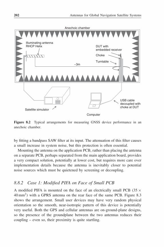
202 Antennas for Global Navigation Satellite Systems
Turntable
DUT withembedded receiver
Illuminating antennaRHCP Helix
Satellite simulator
USB cabledecoupled withchoke at DUT
Computer
~3m
Choke
Anechoic chamber
Figure 8.2 Typical arrangements for measuring GNSS device performance in ananechoic chamber.
by fitting a bandpass SAW filter at its input. The attenuation of this filter causesa small increase in system noise, but this protection is often essential.
Mounting the antenna on the application PCB, rather than placing the antennaon a separate PCB, perhaps separated from the main application board, providesa very compact solution, potentially at lower cost, but requires more care overimplementation details because the antenna is inevitably closer to potentialnoise sources which must be quietened by screening or decoupling.
8.8.2 Case 1: Modified PIFA on Face of Small PCB
A modified PIFA is mounted on the face of an electrically small PCB (35 ×40 mm2) with a GPRS antenna on the rear face of the same PCB. Figure 8.3shows the arrangement. Small user devices may have very random physicalorientation so the smooth, near-isotropic pattern of this device is potentiallyvery useful. Both the GPS and cellular antennas are on-ground-plane designs,so the presence of the groundplane between the two antennas reduces theircoupling – even so, their proximity is quite startling.

Mobile Terminal GNSS Antennas 203
20 30 40 50
0°
90°
180°
270°20 30 40 50
0°
90°
180°
270°GNSS GPRS
Figure 8.3 Case 1: Modified PIFA on face of small PCB. Platform dimensions:35 × 40 mm2. Smooth radiation patterns, with good sky coverage. Note close proximityof the GPRS antenna on the reverse face of the PCB.
8.8.3 Case 2: Meandered Dipole Antenna on Top Edgeof Small PCB
Here a meandered dipole has been positioned at the top of a 55 × 48 mm2
platform to provide it with a clear view of the sky. As may be seen in Figure 8.4,this design feature has failed to ensure that the radiation pattern is dominantly
20 30 40 50
0°
90°
180°
270°20 30 40 50
0°
90°
180°
270°
Figure 8.4 Case 2: Meandered dipole antenna on top edge of small PCB. Plat-form dimensions: 55 × 48 mm2. Patchy upward coverage with higher gain in lowerhemisphere.

204 Antennas for Global Navigation Satellite Systems
upward looking. The positioning of the antenna, combined with the dimensionsof the platform, has resulted in an irregular radiation pattern with significantminima in the upper hemisphere and high sensitivity in a generally downwarddirection. To safeguard against this outcome, the designer should either conductsome simple pattern measurements using a very rudimentary physical modelof the platform – perhaps no more than an unetched PCB, an antenna, batteryand display – or model the simplified structure and antenna using one of theavailable computer simulation packages.
8.8.4 Case 3: Modified PIFA above LCD Display onSmart-Phone-Size Device
This is an example of a platform of typical smartphone dimensions with theantenna mounted centrally above the LCD display. The initial disappointingperformance (Figure 8.5, dashed line) was corrected by removing some ofthe groundplane below the antenna (solid line). The pattern minimum in thedirection orthogonal to the display is probably unhelpful for operation with thedevice lying on a horizontal surface, but is probably caused by the display panel,which occupies much of the face of the PCB. Adjustments to the groundingpositions on the display panel and the battery may also be helpful in optimisingthe radiation pattern.
20 40 50
0°
90°
180°
270° 20 30 40 50
0°
90°
180°
270°30
Figure 8.5 Case 3: Modified PIFA above LCD display on smart-phone-size device(dashed line) showing effect of partial groundplane removal under antenna (solid line).Platform dimensions: 55 × 110 mm2, with battery in place behind PCB. Patchy upwardcoverage with higher gain in lower hemisphere.

Mobile Terminal GNSS Antennas 205
90°50403020270°
Radial Scale: 5 dB-Hz/div Radial Scale: 5 dB-Hz/div0°
180°
90°50403020270°
0°
180°
Figure 8.6 Case 4: Changes in radiation pattern of the modified PIFA when theantenna is moved from one corner of the platform to the adjacent corner.
8.8.5 Case 4: Moving Modified PIFA from One to AdjacentCorner of PCB
This is another example with a platform of suitable dimensions for a smartphoneor PDA. In Figure 8.6 we see that moving the antenna from one corner ofthe platform to the adjacent corner – a simple translation with no associatedrotation – has resulted in a radical change in the radiation pattern. In the originalposition (left hand plot) the polarisation was dominantly LHCP in the upwarddirection, with RHCP directed downwards. Moving the antenna changes therelationship between directly radiated fields and the fields created by currentsflowing in the platform; in this example it has corrected the original polarisationso RHCP is now directed upwards.
This example again shows that comparatively simple experiments early inthe design process can avoid substantial costs for later redesign.
8.8.6 Cases 5 and 6: Effects of Platform Electronics Noise
In Figure 8.7a we see the C/N0 characteristics of a well-designed device with theplatform firmware off (dashed line) and on (solid line).There is very little differ-ence between the two conditions because platform noise has been well controlled.
In Figure 8.7b we see an example of poor noise design. The generallysatisfactory response when the platform electronics is turned off (solid line)collapses to a very unsatisfactory response when the platform electronics isturned on. The sensitivity has fallen by around 25 dB! An expensive respinwill be needed to correct this situation.

206 Antennas for Global Navigation Satellite Systems
30 40 50
0°
90°
180°
270°
(a)
20 30 40 50
0°
90°
180°
270°
(b)
Figure 8.7 Extreme examples of performance with the platform electronics turned on(solid line) and off (dashed line): (a) Near-perfect example with no significant platformnoise; (b) Example with high level of platform noise such that sensitivity is reducedby almost 25 dB.
8.9 Summary
In this chapter we have seen how simple low-cost antennas can provide ade-quate performance for use on a variety of handheld terminals, trackers andother simple devices. Success is achieved by using a well-designed antenna,siting it appropriately on the application and controlling locally generated noiseby good PCB design.
References1. Pathak, V., Thornwall, S., Krier, M. et al., ‘Mobile handset system performance comparison
of a linearly polarized GPS internal antenna with a circularly polarized antenna’, Antennasand Propagation Society International Symposium, Vol. 3, 22–27 June 2003, pp. 666–669.
2. Wingfield, A. and Leisten, O.P., ‘Performance evaluation of small antennas for GlobalPositioning System (GPS)’, Twelfth International Conference on Antennas and Propagation(ICAP), IEE Conference Publication No. 491, 2003.
3. UK Patent GB 2,459,020, Antenova Ltd.

Appendix A
Basic Principle of DecodingInformation from a CDMASignal
Figure A.1 shows how a spreading code of order 4 can be produced for apair of messages to be sent via a CDMA link. This example is for illustrationonly, as 4 bits is not a practical length of code. Figure A.2 shows how thereceived signal (effectively the sum of the two signals from Figure A.1) canbe decoded to reveal the two messages. The ‘correlation’ process is to takethe spreading code used to encode the message to be decoded (in the caseof GPS it is the spreading code for a particular satellite) and multiply it bythe received signal. Over the length of the spreading code the result is thenintegrated and divided by the length of the spreading code and if a messageexists a non-zero result is achieved. In the example in the second row ofFigure A.2 the message (+1, −1, +1) is successfully decoded. In a similarway the message sent via the second spreading code is decoded correctly inthe third row of Figure A.2. In the fourth row of Figure A.2 another spreadingcode (which was not used to encode anything) is used and correctly shows anull message.
This is a very simple illustration and assumes that the spreading code and thereceived signal are synchronised (i.e. the start of the spreading code matchesthe start of a message frame). However, synchronisation is simply achieved
Antennas for Global Navigation Satellite Systems, First Edition.Xiaodong Chen, Clive G. Parini, Brian Collins, Yuan Yao and Masood Ur Rehman.© 2012 John Wiley & Sons, Ltd. Published 2012 by John Wiley & Sons, Ltd.

208 Antennas for Global Navigation Satellite Systems
- 2 Data signals M1(t) = +1−1+1 M2(t) = +1+1−1
- Signal 1 has spreading code of −1−1+1+1
- Signal 2 has spreading code of −1+1+1−1
Time
Time
Time
Time
Time
Time
M1(t)= +1−1+1
C1(t)= −1−1+1+1
T1(t)=M1(t)*C1(t)
M2(t)= +1+1−1
C2(t)= −1+1+1−1
T2(t)=M2(t)*C2(t)
Tb 2Tb 3Tb
Tb 2Tb 3Tb
Tb 2Tb 3Tb
Tb 2Tb 3Tb
Tb 2Tb 3Tb
Tb 2Tb 3Tb
4Tc
Figure A.1 Forming a simple CDMA signal with a spreading code of order 4.
by delaying the spreading code by one chip and recorrelating a frame until anon-null message is received or N delays have been undertaken where N isthe length of the gold code. This is a process that can be rapidly undertakeneven for large spreading codes by a digital signal processor.

Appendix A 209
Time
Time
Time
Time
S(t)=T1(t)+T2(t)
S(t)*C1(t)
S(t)*C2(t)
S(t)*(+1−1+1−1)
Tb 2Tb 3Tb
Tb 2Tb 3Tb
Tb 2Tb 3Tb
Tb 2Tb 3Tb
Row 1- CDMA signal received (sum of the two signals from Figure A1.1)
Row 2- Multiply by spreading code of signal 1
Row 3- Multiply by spreading code of signal 2
Row 4- Multiply by another spreading code
Integrate over0 to Tb
Integrate over0 to Tb
Integrate over0 to Tb
4 −4 4
4 4 -4
0 0 0
Figure A.2 Receiving the CDMA signal.

Appendix B
Antenna Phase Characteristicsand Evaluation of Phase CentreStability
The phase centre of a practical antenna varies in different azimuth and elevationangles, a phenomenon called phase centre dispersion. The antenna phase centrecan only be kept relatively stable within a certain range of directions. Theconcepts of average phase centre, phase centre offset and phase centre variationare introduced to describe fully the characteristics of antenna phase response.
The average phase centre of an antenna is defined as the mean locationof the antenna phase centre over a certain range of directions. The antennareference point (ARP) is defined as the geometric centre of the antenna. Thedifference between the average phase centre and the antenna reference pointis regarded as the phase centre offset (PCO). The offset between the phasecentre in a particular direction and the average phase centre is known as phasecentre variation (PCV) in that direction. These three parameters are illustratedin Figure B.1.
Typical antenna installations for surveying use the ARP as the reference pointfor phase measurements, so a correction must be made to allow for the PCOin the direction of the satellite signals. The average phase centre, or PCO, canbe found by minimising the cost function:
∑(PCV)2 = Min
In order to improve the reliability and accuracy of the GNSSs, we have to takeinto consideration the effect of antenna phase centre stability.
Antennas for Global Navigation Satellite Systems, First Edition.Xiaodong Chen, Clive G. Parini, Brian Collins, Yuan Yao and Masood Ur Rehman.© 2012 John Wiley & Sons, Ltd. Published 2012 by John Wiley & Sons, Ltd.

212 Antennas for Global Navigation Satellite Systems
r
PCO
ARP PCO∗r0
PCV(φ,θ)
r
PCV
Signal
direction r0
Figure B.1 Illustration of ARP, PCO and PCV [1]. Reproduced by permission of© 2010 IEEE.
B.1 Evaluation of Phase Centre Stability
As shown in Figure B.1, we can use the average phase centre as the originto calculate the PCV as a function of azimuth and elevation angle. The phasecentre stability is defined as half the PCV peak value across the main beam ofthe antenna. It can be expressed as
�m = 1
2· �ϕ
360· λ (B.1)
where �m is phase centre stability, �ϕ is the peak value of PCV and λ is thecorresponding wavelength.
B.2 Determination of the Average Phase Centre
A simple and practical method of computing average phase centre may be basedon either simulated or measured antenna phase patterns [1]. We will use a leastsquares method and start with the equation of spherical phase expansion from itsorigin located at point phase centre (x, y, z) as shown in the equation below.A term c is added that can represent some constant. Azimuth and elevationangles are denoted as θ and φ, and the wavelength is λ. Thus
Phase(φ, θ) = 2π
λ(x · cos φ sin θ + y · sin φ sin θ + z · cos θ) + c

Appendix B 213
or in matrix form
F(φ, θ) = 2π
λ[cos φ sin θ sin φ sin θ cos θ] ·
⎡⎢⎢⎣
x
y
z
c
⎤⎥⎥⎦ (B.2a)
⇒ F = M · P (B.2b)
To find phase centre P , we use Equation B.2b, hence
P = M−1 · F (B.3)⎡⎢⎢⎣
x
y
z
c
⎤⎥⎥⎦ = λ
2π[cos φ sin θ sin φ sin θ cos θ]−1 · F(φ, θ) (B.4)
We are now ready to assemble a solution matrix using either simulated ormeasured data obtained from sampling the phase pattern of the antenna toobtain a mean value of PCO:
⎡⎢⎢⎣
x
y
z
d
⎤⎥⎥⎦ = 1
2π·
⎡⎢⎢⎢⎢⎢⎢⎢⎢⎢⎢⎣
cos φ1 sin θ1 sinφ1 sin θ1 cosθ1 1cos φ2 sin θ1 sinφ2 sin θ1 cosθ1 1
......
......
cos φN sin θ1 sinφN sin θ1 cosθ1 1cos φ1 sin θ2 sinφ1 sin θ2 cosθ2 1
......
......
cos φN sin θK sinφN sin θK cosθK 1
⎤⎥⎥⎥⎥⎥⎥⎥⎥⎥⎥⎦
·
⎡⎢⎢⎢⎢⎢⎢⎢⎢⎢⎢⎣
ϕ1(φ1, θ1) · λ
ϕ2(φ2, θ1) · λ...
ϕN(φN, θ1) · λ
ϕN+1(φ1, θ2) · λ...
ϕN ·K(φN, θK) · λ
⎤⎥⎥⎥⎥⎥⎥⎥⎥⎥⎥⎦
(B.5)
where
φi = 0 : 2π/N : 2π, θi = 0 : π/2K : π/2 (upper hemisphere)
Reference1. Waldemar, K., ‘Antenna phase center effects and measurements in GNSS ranging applica-
tions’, 14th International Symposium on Antenna Technology and Applied Electromagnetics(ANTEM) & the American Electromagnetics Conference (AMEREM), Ottawa, Canada, 5–8July 2010.
Index
absolute impedance bandwidth, 27accuracy (of fix), 187–8, see also
precision of fixactual reflection environment, 128Aeronautical Radio, 15angular density function, 114antenna(s)
active, 185–7external, 186Galileo, 41–51GPS III, 42groundplane-free, 197helical, 42, 48internal, 186inverted-F, see IFAlinearly polarised, 184on-ground, 197patch, see patch antennaPIFA, see PIFAunbalanced, 183, 192, 197
antenna coverage, 162antenna efficiency, 29antenna orientation, 133, 136antenna phase centre, 17–18, 27antenna position (on platform), 197antenna reference point (ARP),
211
Antennas for Global Navigation Satellite Systems, First Edition.Xiaodong Chen, Clive G. Parini, Brian Collins, Yuan Yao and Masood Ur Rehman.© 2012 John Wiley & Sons, Ltd. Published 2012 by John Wiley & Sons, Ltd.
AR bandwidth, 35–6Archimedean spiral antenna (ASA),
71Assisted GPS, 140average phase centre, 211axial (endfire) mode, 31axial ratio (AR), 29
back lobe, 27bandwidth, 187beamfoming, 141beamwidth, 184Body shielding, 162, 175, 177
calibration data, 188capacitively fed microstrip patch
antenna, 62carrier cycle integer ambiguity, 14,
16carrier phase timing, 13case studies, 201cases, effect of, 197CDMA, 11ceramic chip antenna, 64circular polarisation, 22circularly polarised (CP), 21, 26,
29

216 Index
clear sky view, 113, 135–6,161
Coarse Acquisition code (C/A),11–12
code phase timing, 13cold start, 195comparative trials, 195–6compass, 2–3, 81computer simulation, 204conical spiral, 33coverage efficiency, 117, 120CP microstrip patch, 122, 127cross-polar discrimination, 36Cross-Polarisation Ratio, 115–16
delays, ionospheric, 187detuning, 154, 171–2dielectric resonator antenna (DRA),
96differential GPS, 15dilution of precision, 9dipole, 122, 127dipole antenna, 29direct signal, 133, 136directivity, 28diversity, 141Doppler shift, 7, 14, 24DRA, 124, 151drive test, 194dual-feed CP patch antenna, 34dual-feed microstrip GNSS antennas,
60dynamic range, 186–7
efficiency, 186, 193electromagnetic (EM), 21elliptical polarisation, 22elliptically polarised (EP), 26, 29environment, 111equivalent phase centre, 28
error budget : GPS C/A codepseudo-range, 16
ETSI, 140
Faraday rotation, 25FCC, 149flat spiral antenna, 32fractional impedance bandwidth, 27free space loss, 118frequency-dependent phase shift
(group delay), 25
gain, 28, 186Galileo, 1, 3, 81generalised scattering matrix (GSM),
45GLONASS, 1, 3, 81GNSS, 21, 55GPS, 81GPS Angle of Arrival Distribution,
116GPS constellation, 5GPS link budget, 118GPS Mean Effective Gain, 114GPS Receiver, 13ground reflections, 116–17, 133,
160groundplane, 193, 197group delay, 44
half-power beamwidth (HPBW), 27helical antenna, 31helix, 125, 151helix, quadrifilar, 190human body, 149human body model, 167
IFAs (Inverted-F Antennas), 39, 123,192
impedance, 185, 192

Index 217
impedance bandwidth, 27input impedance, 158interference, 39, 182–3, 185ionosphere, 24ionospheric corrections, 14ionospheric dispersion, 25ionospheric effects, 25
left hand circular polarisation(LHCP), 22, 26, 112
linear polarisation, 22linearly polarised (LP), 25, 29line-of-sight, 111loop antenna, 192low-noise amplifier (LNA), 39, 187,
194, 196, 201
main beam, 27major lobe, 27mean effective gain, 113, 150mean incident power, 114, 120mean received power, 114, 120microstrip antenna, 55minor lobes, 27mismatch efficiency, 151mobile terminal, 141mono-loop, 126multiband terminal antennas,
81multi-layer body model, 166multimode antennas, 81multipactor effect, 52multipath, 25, 111, 149multipath environment, 116multipath signal, 133, 136muscle tissue, 167mutual coupling, 145
navigation Service (ARNS), 15NAVSTAR, 1, 3
no reflection environment, 128noise
broadband, 182conducted, 185out-of-band, 194platform, 181, 193, 200, 205radiated, 185
noise figure, 186noise floor, 193non-dispersive, 25non-line-of-sight, 112NTIA, 140numerical model, 150
open field, 117open field test, 119
paint, effect of, 197passive intermodulation (PIM), 50patch antenna, 33, 191, 192penetration depth, 166perfectly matched layer, 152phase centre, 81, 188phase centre dispersion, 211phase centre offset (PCO), 211phase centre variation (PCV), 211phase characteristic, 188phase pattern, 27, 28PIFAs (Planar Inverted-F Antennas),
39, 55, 122–3, 127, 151, 201plane wave, 21platform
geometry of, 192position on, 192
polarisation, 29, 182, 193effective, 183
polarisation loss factor (PLF), 29polarisation matching, 186polarisation mismatch, 29portable devices, 112
218 Index
precision (of fix), 182, see alsoAccuracy of fix
precision positioning service(PPS), 11
precision, dilution of, 182propagation, 21pseudo-range error, 25
quadrifilar helical antennas, 66quadrifilar helix antenna (QHA), 88QZSS, 2–3
radiation efficiency, 29radiation pattern(s), 27, 181, 184,
190, 191–3, 204–5measurement of, 184Galileo, 45–7
Radio Technical Commission forMaritime Services, 15
radio waves, 21, 149realised gain, 151receiver sensitivity, 118reflected fields, 159reflection (mismatch) efficiency,
29reflection coefficient, 116refraction, 25reliability (of fix), 188right hand circular polarisation
(RHCP), 22, 26, 55
satellite simulator, 185, 197SAW filter, 185, 193, 202sensitivity, 190signal reradiation, 140
signal-to-noise ratio, 119, 121single-feed CP microstrip antennas,
55single-feed CP patch antenna, 34sky view, limited, 190solid angle, 117–18specification parameters, 183spiral antenna(s), 71, 32standard positioning service (SPS),
11statistical model, 113
telemetry tracking and command(TT&C), 10
terminalsgeodetic, 189handheld, 189rover, 189
terminal antennas, 55time to first fix (TTFF), 140, 190,
194, 200tissues, 152tissue electrical properties, 154total electron content (TEC), 24total reflection environment, 128transmitters, co-sited, 193troposphere, 25
voltage standing wave ratio(VSWR), 27, 186
voxels, 152
WBAN, 149wideband microstrip antenna, 95WPAN, 149