Embed Size (px)
Citation preview

DWSS ndash Part 1 Ch1 - Properties of Fluids and Pipes 11022014
Ch1 exo - 13
Answers to basic exercises
1 What is the mass of 1 dm3 of mercury The volume is V = 10-3 m3 The relative density is 135 The density of mercury in kgm3 is the product of its relative density and the density of water in kgm3 (135) times (103) = 13500 kgm3 From Eq 1-1 the mass is given by m = ρ ∙ V = 13500 times 10-3 = 135 kg
2 What is the density of sea water at 5degC knowing that the average salinity is 35 grams per litre The volume of 1 litre of seawater is V = 1 times 10-3 m3
The mass of 1 litre of seawater is 1 kg plus 0035 kg m = 1035 kg The density from Eq 1-1 is ρ = m V = 1035 10-3 = 1035 times 103 kgm3
The addition of salt has a similar influence on density as a decrease in temperature salty water at 20degC will have the same density as pure water at 5degC
3 What is the density of air at a pressure of 1 ∙ 105 Pa and a temperature of 30degC The pressure is P = 105 Pa The gas constant for dry air is R = 293 mK The absolute temperature is about T = 273 + 30 = 303 K
Standard gravity is g = 981 ms2
The density of air is given by Eq 1-2 ρ = 105 (293 times 303 times 981) = 115 kgm3
Thus one litre air is about one thousand times lighter than a litre of water
4 In a closed air tank we have a pressure of 10 ∙ 105 Pa at 0degC As the maximum pressure authorised for the vessel is 12 ∙ 105 Pa what is the maximum temperature admissible The pressure at 0degC is P0 = 10 times 105 Pa The ma∙ pressure is Pma∙ = 12 times 105 Pa The absolute temperature at P0 is T0 = 273 K
The tank is considered as closed and rigid therefore V0=Vma∙ With the Eq 1-3 P0 ∙ V0 T0 = Pma∙ ∙ Vma∙ Tma∙
=gt Tma∙ = Pma∙ ∙ T0 P0 = 12 times105 times 273 10 times105 = 3276 K or Tma∙ = 546 degC
The maximum pressure could be easily attained through temperatures that could realistically occur in a confined enclosure
5 What is the water density under an increase of 30∙105 Pa at 5degC The mass of 1 m3 of water is 1000 kg The bulk modulus for water is KWater = 22 times109 Pa
The volume of 1 m3 of water under 30 times 105 Pa will decrease according to Eq1-4 =gt ΔV = ΔP ∙ V0 KWater = 30 times105 times1 22 ∙109 = 00014 m3
The volume of 1000 kg of water at 30 ∙ 105 Pa is therefore 1-00014 = 09986 m3
The density according to eq 11 ρ = m V = 1000 09986 = 1 0014 kgm3
Note that the increase of density due to a huge pressure (30times105 Pa) has a similar effect as an increase of 15deg of temperature
Answers to intermediary exercises
6 What is the reduction of volume of a 1m3 steel cube under an increase of 20 ∙105 Pa The variation of pressure is ΔP = 20 times 105 Pa
The bulk modulus for steel is Ksteel = 160 times109 Pa
The initial volume is V0 = 1 m3
DWSS ndash Part 1 Ch1 - Properties of Fluids and Pipes 11022014
Ch1 exo - 23
With the Eq 1-4 we find ΔV = ΔP ∙ V0 KSteel = 20 times105 times 1 (160 times109) = 125 times10-6 m3 = 125 cm3
The maximum pressure could be reached with a temperature that could be easily found in certain condition like in a closed building without aeration
7 What is the phase of the water at 5∙105 Pa and 0degC
8 What will be the length and diameter of a PE pipe (original length 20m original diameter 200mm) after thermal expansion due to temperature changing from 5degC to 25degC
For the length we have the following formula ΔL=LmiddotΔTmiddotαT
the length is L=20 m the temperature variation is ΔT=25-5=20deg the thermal expansion coefficient for PE is αT=02 mmmdegK ΔL= 20times20times02=80 mm=008 m
the final length is Lf = Li+ΔL=20+008=2008 m
For the diameter we have ΔD=DmiddotΔTmiddotαT
the diameter is L=01 m the temperature variation is ΔT=25-5=20deg the thermal expansion coefficient for PE is αT=02 mmmdegK ΔD= 01times20times02=04 mm
Therefore the final diameter is Df=Di+ ΔD=100 + 04 mm=1004 mm In fact the thermal expansion of the diameter is negligible since it is almost as much as the error margin for PE pipe
9 A plate 50 x 50 cm is supported by a water layer 1 mm thick What force must be applied to this plate so that it reaches a speed of 2ms at 5degC and at 40degC
The viscosity of water at 5degC is according to table 1 μ5degC = 1519 times10-3 Pa∙s The viscosity of water at 20degC is according to table 1 μ20degC = 0661 times 0992 ∙ 10-3 = 0656times10-3 Pa∙s The surface of the plate is A = 05 times 05 = 025 m2 The velocity is v = 2 ms The distance between the plates is y = 0001 m
Water
Water vapour
Ice
105
221times105
611
0 01 100 374
Temp degC
Triple point
bull
bull
Critical point
Pressure
[Pa]
bull
The state is liquid
5times105
DWSS ndash Part 1 Ch1 - Properties of Fluids and Pipes 11022014
Ch1 exo - 33
With the Eq 1-6 we find the force to be applied at 5degC F = 1519 times 10-3 times 025 times 2 0001 = 0760 N
at 40degC F = 0656 times 10-3 times 025 times 2 0001 = 0328 N
The viscosity of the water is quite small as with a force of 76 grams we can move the plate and at 40degC half of this force is necessary
Answers to the advanced exercises
10 What is the increase of diameter of PE pipe of outside diameter 200 mm and thicknesses of 91 mm 147 mm 224 mm at 10∙105 Pa The variation of pressure is ΔP = 10 times 105 Pa
The bulk modulus for PE is KPE = 12 times109 Pa
The diameter is D = 02 m
The thicknesses are e1 = 00091 m e2 = 00147 m e3 = 00224 m
With the Eq 1-5 we find
With e1 ΔD D = 10times105 (12times109) times02 (2 times 00091) = 09
With e2 ΔD D = 10times105 (12times109) times 02 (2 times 00147) = 06
With e3 ΔD D = 10times105 (12times109) times02 (2 times 00224) = 04
The increase of the pipe diameter even with the thinner one is smaller than the construction tolerance
11 the following three dimensional chart (PTV) representation of the phase element find the following
Critical point amp triple point (line)
Plain water ice vapour supercritical fluid
Mixed water amp ice water amp vapour ice amp vapour
Vapour
Ice
Water Supercritical fluid
Ice amp vapour Water amp vapour
Ice amp water
Critical point
Triple point (line)
DWSS ndash Part 1 Ch2 - Hydrostatics 11022014
Ch2 exo - 12
Answers to basic exercises
1 What is roughly the pressure an 80kg man exerts on the ground
From Eq2-1 the pressure is given by P = F A
In this case F is the gravity force F = m ∙ g = 80 times 981 = 7848 N
The surface A is the sole of the 2 feet So approx A = 2 times 025 times 015 = 0075 m2
So P = 10 464 Pa Only 10 additional to the Atmospheric Pressure (101 325 Pa) it might change a lot with the shape of the soles
2 What is the water pressure at the bottom of a pool 15 m deep at 5degC and at 25degC
From Eq2-6 Pbottom = ρ ∙ g ∙ h
At 5degC ρ = 1000 kgm3 P bottom = 147 150 Pa
At 25degC ρ = 9971 kgm3 P bottom = 146 723 Pa
At both temperatures it remains close to 15 mWC
Answers to intermediary exercises
3 What is the average atmospheric pressure at your place and at 4000 masl
At sea level (0 masl) the atmospheric pressure is 1 013 hPa In Pyong Yang elevation is 84masl From Eq2-3 Pressure (84 masl) = 1 003 hPa so 1 variation from the pressure at sea level At 4 000 masl Pressure (4000 masl) = 616 hPa so 39 variation from the pressure at sea level
4 At 4000 masl what is the elevation of a column of mercury and a column of water
From Eq2-2 the height of the mercury column is given by h = Pa ρ ∙ g
As seen in question 2 the Pa at 4 000 m is Pa = 61 645 g is assumed as 981 ms2 With mercury density ρ is 13 500 kgm3 At 4 000 masl h = 047 m
For water if the effect of the vapour pressure is neglected (at low temperature) the same equation can be used With water density is 1 000 kgm3 At 4 000 masl h = 628 m To be compared with 10 m at
sea level
5 What is the maximum suction height for water at 30degC at 1500 masl
From Eq2- 3 Pa (1500 masl) = 84559 hPa (83 of Pa at sea level)
From the graph Pv = 000000942 ∙ t4 - 0000291 ∙ t3 + 00331 ∙ t2 + 0242 ∙ t + 611
Pv (30deg) = 43 hPa
From Eq2-4 the maximum pumping height is given by h = (Pa-Pv) ρ (30deg) ∙ g
so h = ( 84 559 ndash 4 300 ) (9957 times 981) = 822 m
6 What is the maximum suction height for water at 15degC at 3000 masl
Following the same path than question 5 we have Pa (3000 masl) = 70112 hPa
Pv (15deg) = 17 hPa ρ (15deg) = 9991 Thus h = 698 m
DWSS ndash Part 1 Ch2 - Hydrostatics 11022014
Ch2 exo - 22
7 What is the buoyant force applied to a body of 2 m3
From Eq27 F = ρ ∙ g ∙ V
The nature of the body is not of importance but the nature of fluid is important If it is water ρ is 1 000 Kgm3 F = 1000 times 981 times 2 F= 19 620 N If it is mercury ρ is 13 500 Kgm3 F = 13500 times 981 times 2 F= 264 870 N
Answers to the advanced exercises
8 A water pipe has its top at 500 mASL and its bottom at sea level What is the variation of atmospheric pressure between the top and the bottom What is the water pressure at the bottom What is the ratio between these two pressures
From Eq2-3 Patm(0 mASL) = 101 325 Patm(500 mASL) = 95 462 =gt ΔPatm (0 to 500 mASL) = 5 863 Pa
From Eq2-5 Pwater = ρ ∙ g ∙ h = 1 000 times 981 times 500 = 4 905 000 Pa The ratio is Pwater ΔPatm = 836 The water pressure is much more important than the variation of air pressure therefore difference of atmospheric pressure due to the variation of altitude can be neglected in water systems
9 What is the force applied by the liquid to the side of a water tank that is 2 m high and 10 m wide
The pressure is nil at the top and increases linearly till the maximum at the bottom The average can therefore be taken at the centre From Eq2-6 P = ρ ∙ g ∙ h
The centre of the side of the tank is at 1m down So at 1m depth Pw = 981 times 103 Pa From Eq2-1 P =FA Thus F = P ∙ A
The surface of the side of the tank is A = 10 times 2 m2 At the centre of the side of the tank F = 19620 kN It weighs as a truck of 196 tons
10 What is the buoyant force exerted on an 80 kg man by the atmosphere
From Eq2-7 F = ρ ∙ g ∙ V
In Chapter 1 question 3 we have calculated the density of air at 1times10 5 Pa and 30degC =gt ρ = 115 kgm3 The density of a human body is close to the water density (as we are almost floating in water) thus Eq1-1 =gt V = m ρ = 80 103 = 008 m3
With g = 981 ms2 the buoyant force from atmosphere is F = 115 times 981 times 008 = 090 N The gravity force is F = m ∙ g = 7848 N hellipThat is why we do not float or fly
11 An air balloon of 1m3 at atmospheric pressure is brought at 10m below water surface what will be the buoyant force And at 20m below water surface
The volume of the balloon can be calculated with the ideal gas law (Eq 1-3) the temperature can be considered as constant thus P ∙ V = constant At 10m below water surface the pressure is twice the atmospheric pressure thus the volume will be half =gt V10m=Vsurface ∙ Psurface P10m = 1 times 1 2 = 05 m3 From Eq2-7 F = ρ ∙ g ∙ V = 103 times 981 times 05 = 4 905 N
At 20m below water surface the water pressure will be about 2 atm and total pressure 3 atm thus =gt V20m=Vsurface ∙ Psurface P20m = 1 times 1 3 = 0333 m3 From Eq2-7 F = ρ ∙ g ∙ V = 103 times 981 times 0333 = 3 270 N
DWSS ndash Part 1 Ch3 Hydrodynamics 11022014
Ch3 exo - 13
Answers to basic exercises
1 What is the flow in a pipe of 150mm of diameter with a 1ms speed
The section area is A = π ∙ D2 4 = 31415 times (015)2 4 = 001767 m2
The mean velocity is v = 1 ms
With the Eq 3-2 the flow is Q = A ∙ v = 001767 times 1 = 001767 m3s = 177 ls
2 What is the speed in the same pipe after a reduction in diameter to 100mm and to 75mm
From Eq 3-2 Q = A ∙ v = (π D2 4) ∙ v and Q is constant Q1 = Q2 = A2 ∙ v2
After reduction to a pipe of 100 mm of diameter v2 = Q1 A2 So v2 = 225 ms After reduction to a pipe of 75 mm of diameter v3 = Q1 A3 So v3 = 4 ms With a reduction of 50 in diameter the speed is increased by 4
3 What is the flow in the same pipe after a Tee with a 25mm pipe with a 1 ms speed
From Eq 3-3 Q1 = Qtee + Q2 =gt Q2 = Q1 - Qtee Qtee = (π D2 4) ∙ v so Qtee = 0000491 m3s = 049 ls
So the flow after the tee will be Q2 = 177 ndash 049 = 172 ls
4 What is the speed of water going out of the base of a tank with 25m 5m and 10m height
If we neglect the losses applying the Law of Conservation of Energy the speed of the water is given by v = radic 2 ∙ g ∙ h
For h = 25 m v = 7 ms For h = 5 m v = 99 ms For h = 10 m v = 14 ms
When multiplying the height by 4 the speed is multiplied by 2 only
5 What are the speed and the flow in a pipe of 150mm of diameter showing a difference of 20cm height in a Venturi section of 100mm diameter
In Eq 3-6 A1A2 = (D1D2)2 with D1 = 015 m D2 = 010 m amp h = 020m =gtv1 = radic(2 times 981 times 02 ((015 01)4-1))) = 0983 ms
From Eq 3-2 Q1 = (π D12 4) ∙ v1 = 31415 times 0152 4 times 0983 = 1736 ls
Answers to intermediary exercises
6 What are the Reynolds numbers for the flows in the exercises 12 amp 5
From Eq 37 Re = D middot v ν
D (m) v (ms) ν (m2s) Re
0150 100 1E-06 150 000
0100 225 1E-06 225 000
0075 400 1E-06 300 000
0150 098 1E-06 147 450
It can be noted that we are always in turbulent conditions
DWSS ndash Part 1 Ch3 Hydrodynamics 11022014
Ch3 exo - 23
7 For a pipe of 150mm of diameter with 2 bar pressure a velocity of 1 ms what should be the diameter reduction to cause cavitation at 20degC (neglect head losses)
With Eq 3-4 as the elevation is the same H1 = H2 we can neglect the head losses and dived all terms by g
2
vv
ρ
PP
2
v
ρ
P
2
v
ρ
P 2
1
2
221
2
22
2
11
Furthermore with Eq 3-2 we found v2 according to v1
2
1122211ii
A
AvvAvAvcteAvQ
To have cavitation the total pressure should be at Pv ie the water pressure should the vapour pressure (2 400 Pa at 20degC)
2
1
2
1
21
2
2
12
1
21
2
1
2
221
A
A1
vρ
PP2
2
1A
Av
ρ
PP
2
vv
ρ
PP
1
222
2
2
1
2
1
A
AD1D
D
D
A
A
P1 = 200 000Pa P2 = 2 400 Pa We find A1A2 = 199 and D2 = 336 [mm]
Answers to advanced exercises
8 With equations Eq 2-5 Eq 3-2 amp Eq 3-4 demonstrate Eq 3-6
As for the previous exercice with Eq 3-4 as the elevation is the same H1 = H2 we can neglect the head losses and dived all terms by g we have
2
vv
ρ
PP
2
v
ρ
P
2
v
ρ
P 2
1
2
221
2
22
2
11
With Eq 3-2 we found v2 according to v1 2
1122211ii
A
AvvAvAvcteAvQ
With Eq 2-5 we found the difference of pressure
ΔhgρhhgρPPhgρPP 2121atmtot
Inserting these elements in the first equation
1A
AvΔhg2
2
v-A
Av
ρ
Δhgρ2
2
12
1
2
1
2
2
11
Thus we find Eq 3-6
1
A
AΔhg2v
2
2
11
DWSS ndash Part 1 Ch3 Hydrodynamics 11022014
Ch3 exo - 33
9 For a pipe of 150mm of diameter with 1 bar pressure a velocity of 1 ms what should be the diameter reduction to cause air suction
We suppose that elevation is the same thus H1=H2 and losses are neglected To have air suction the total pressure should be at Patm ie the water pressure should be nil Similar formulas as for the previous exercise give the following
2
1
2
1
21
2
2
12
1
21
2
1
2
221
A
A1
vρ
PP2
2
1A
Av
ρ
PP
2
vv
ρ
PP
1
2122
2
2
1
2
1
A
ADD
D
D
A
A
Thus with P1= 100 000 Pa v1 =1 ms we find A1A2 = 14 and D2 = 40 [mm] In reality the head losses can not be neglected and the actual value will be bigger this will be seen in the next chapter
10 A tank of 2m high and 1m diameter has a 75mm valve at the bottom When the tank is full and the valve is quickly opened how long does it take to empty the tank (the losses and contraction factor are neglected)
There is 2 ways to resolve this exercise
A) Through a differential equation
The flow going out of the tank is 2ghAQ valve
The variation of height of the water level in the tank is tA
Qh
Tank
Combining the two equations and rearranging th2ghA
A-t
A
2ghAh
valve
Tank
Tank
valve
This equation can be integrated
h2
h1
21
valve
Tank
h2
h1 valve
Tank
2
1
hh2gA
A-h
2ghA
A-t
t
t
The final results is then
gA
hh2A
2gA
hh2A-ttt
valve
21
2
21
1Tank
valve
21
12Tank
12
Thus with h2=0 h1=2 Atank = 0785 Avalve=00044 we find t = 114 s
B) Easier way but only working if the diameter of the tank is constant
It will take the time to empty the tank at the average velocity
2
2ghV02
2V avg
21avg
V
VV
DWSS ndash Part 1 Ch4 Flow in pipes under pressure 11022014
Ch4 ndash Exo 15
Answers to basic exercises
1 What are the ID the SDR and the Series of a pipe with an outside diameter of 110 mm and a thickness of 66 mm
Using OD = 110 mm and e = 66mm From Eq 4-2 ID = OD ndash 2e ID = 110 - 2 times 66 ID = 968 mm From Eq 4-3 SDR = OD e SDR = 110 66 SDR = 1667 rounded to 17 From Eq 44 S = (SDR-1)2 S = ((11066) -1)2 S = 783 rounded to 8
2 What is the nominal pressure of this pipe if it is made with PVC and used at a temperature of 30degc If it is made with PE80 PE100 at 20degC
From Eq 45 PN = 10 MRS (S C) For a diameter 110 in PVC MRS = 25 MPa and C=2 For temperature lower that 25 degC PN = 10 (25 (8times2) PN = 16 bar But 30degC the derating temperature factor (ft) is = 088 So finally PN is only 14 bar
For a diameter 110 in PE 80 at 20degC MRS = 8 and C= 125 (no derating factor) From Eq 45 PN = 10 times 8 (8 times 125) PN = 8 bar
For a diameter 110 in PE 100 at 20degc MRS = 10 and C= 125 (no derating factor) From Eq 45 PN = 10 times 10 (8 times 125) PN = 10 bar
3 What is the nominal pressure of these PE pipes if it is used for gas (the service ratio is 2 for gas)
For a diameter 110 in PE 80 at 20degc MRS = 8 and C= 2 (no derating factor) From Eq 45 PN = 10 times 8 (8 times 2) PN = 5 bar
For a diameter 110 in PE 100 at 20degc MRS = 10 and C= 2 (no derating factor) From Eq 45 PN = 10 times 10 (8 times 2) PN = 6 bar
4 What are the friction losses in a DN150 PVC pipe of 22 km with a velocity of 1 ms Same question for a cast iron pipe (k=012mm) (can be estimated with figures either log scale of charts in annexes)
PVC pipe
With the charts (taking the chart for k=0005) for a pipe of diameter 150mm and a velocity of 1 ms the result is 056 m100m Given that we have a pipe 22 km long HL= 056 times 22 =123 m
Steel pipe
With the charts (taking the chart for k=012) for a pipe of diameter 150mm and a velocity of 1 ms the result is 07 m100m Given that we have a pipe 22 km long HL= 07 times 22 =154 m
Answers to intermediary exercises
5 What is the hydraulic diameter of a square pipe (b=h) Of a flatten (elliptic) pipe with b=2h
For the square pipe From Eq 47 A = h2 and P = 4h so in Eq 46 Dh = 4 AP Dh= h
For the flatten pipe From Eq 48 A = π h2 2 and P = 3 π h 2 so Dh = 4 AP Dh = 4h 3
6 What is the minimum velocity and flow that should flow to avoid air pocket (Re = 10000) in a pipe of DN25 DN200 DN500
DWSS ndash Part 1 Ch4 Flow in pipes under pressure 11022014
Ch4 ndash Exo 25
From Eq = 49 Re = D middot v ν so v =Re middot ν D
When Re = 10000 the minimum velocity is reached When D = 0025 m v = 10000 times 0000001 0025 v = 04 ms The flow will then be Q = π D2 middot v 4 Q= 314 x (0025) 2 x 04 4 Q= 0196 ls
When D = 02 m v = 10000 0000001 02 v = 005 ms The corresponding flow will be 157 ls When D = 05 m v = 10000x 0000001 05 v = 002 ms The corresponding flow will be 392 ls
7 What is the punctual friction losses coefficient for a pipe connected between to tanks with four round elbows (d=D) a gate valve a non-return valve and a filter
4 round elbows (d=D) Kp = 4 times 035
1 gate valve Kp = 035
1 non-return valve Kp = 25
1 filter Kp = 28
1 inlet Kp = 05
1 discharge Kp = 15 The punctual friction losses coefficient is the sum Kptotal = 905
8 What is the average punctual friction losses coefficient for the accessories of a DN200 pump
A classical setup includes the following items
foot valve with strainer Kp = 15
3 round elbows (d=D) Kp = 3 times 035
1 reduction (dD=08 45deg) Kp = 015
1 extension (dD=08 45deg) Kp = 01
1 gate valve Kp = 035
1 non-return valve Kp = 25 The punctual friction losses coefficient is the sum Kptotal asymp 20 three quarter are due to the foot valve this is usually the most critical part
9 What are the friction losses in a DN150 PVC pipe of 22 km with a velocity of 1 ms Same question for a steel pipe (k=1mm) (to be calculated with equations not estimated with charts)
The Reynolds number is Re = Dmiddotvν Re = 150000
For a PVC pipe the flow will be turbulent smooth From Eq 418 λ = 0309 (log (Re7))2 = 00165 From Eq 415 and kL = λ LD= 00165 times 2 200015 = 2416 From Eq 410 and HL= kLv22g = 123 m
If we compare this result with the one obtained in exercise 4 we see that the results match approximately However the method used in exercise 4 are usually less precise For a DN 150 steel pipe the flow will be turbulent partially rough The ratio kD = 1150 = 0007 From Eq 417 λ = 00055+015(Dk)(13) = 0033 with Eq 419 λ = 0034 thus taking rough instead
of partially rough underestimate the losses From Eq 415 and kL = λ LD= 0034 times 2 200015 = 498 From Eq 410 and HL= kLv22g = 254 m
10 What should be the diameter of an orifice to create losses of 20 meters in a DN100 pipe with a velocity of 1 ms
For an orifice we can use Eq 4-14 K p-o = H P Orifice middot 2g v1
2
with H P Orifice = 20 m and v1 = 1ms K p-o = 391 asymp 400
DWSS ndash Part 1 Ch4 Flow in pipes under pressure 11022014
Ch4 ndash Exo 35
On the chart dD is - if it is a sharp orifice dD = 028 which make d = 28 cm - if it is a beweled orifice dD = 027 which makes d= 27 cm - if it is a rounded orifice dD = 024 which makes d= 24 cm Practically a hole of 24 cm should be done in plate placed between two flanges This orifice can then be filed down to be increased if necessary
Answers to advanced exercises
11 What is the flow in a DN150 galvanised pipe of 800 m connecting two tanks with a gate valve five elbows and a filter if the difference of height between the tanks is 2m 5m 10m
From Eq 4-11 we have HA ndash HB = ∆H = (Q2 ( Kp + Kl) ) (121timesD4)
with D = 015 =gt Q2 = ∆H times 000613 (Kp + Kl) To calculate Kponctual it is necessary to sum all punctual losses the system is composed of
System Kp
1 inlet 05
1 gate valve 035
5 elbows (round) 175
1 filter 28
1 discharge 15
Total Kponctual = 69
To estimate Klinear we calculate the ratio kD = 0001 (D = 150mm and k = 015 m) We can see
in the Moody chart that with this ratio we have a λ between 004 and 002 according to the
Reynolds Let assume a value of 002 (Re gt 800000 turbulent rough) to start Then from Eq 4-15 Klinear = λ LD = 002times800015 = 1067
Then we can calculate the flow Q2 = 2 times 000613 1136 =gt Q= 00104 m3s or 104 ls
The velocity and Reynolds can now be calculated v = 4 middot Q (π times D2) = 059 ms and Re = D middot v ν = 88000
By checking the Moody chart we can see that the λ has roughly a value of 0023 giving a
value of Klinear = 1227 what is not negligible The calculation should be done again with this new value giving Q= 00097 m3s or 97 ls v=055 ms and Re = 83000
This time the Re is close enough to our estimation one iteration was enough to find a precise value
For ∆H = 5m with a λ= 002 we find with the first calculation
Q= 00164 m3s or 164 ls v=093 ms and Re = 140000
For a Re of 140000 lets take a λ=0022 and recalculate Q= 00157 m3s or 157 ls v=089 ms and Re = 133000 what is precise enough
For ∆H = 10m with a λ= 002 we find with the first calculation
Q= 00232 m3s or 232 ls v=131 ms and Re = 197000
For a Re of 197000 lets take a λ=0021 and recalculate
DWSS ndash Part 1 Ch4 Flow in pipes under pressure 11022014
Ch4 ndash Exo 45
Q= 00227 m3s or 227 ls v=128 ms and Re = 192000 what is precise enough
12 How much shall a pipe be crushed to reduce the flow by half
With equation 4-11 we know that 4
LP2
LPBAD
k
121
QHH-H (1)
Given that HA-HB is constant we have 4
1
LP
2
1
D
k
121
2)(Q= 4
2
LP
2
2
D
k
121
)(Q (2)
We assume that λ does not vary significantly with the change occurring after the crushing Furthermore we have kLP = λmiddotLD (3) Putting (3) into (2) and multiplying both sides by 121 we get
5
1
2
1
D
Lλ
4
Q5
2
2
2D
LQ
(4) Which gives us 5
1D
1
5
2D
4 (5) so at the end
75804
1
D
D51
2
1
(6) It is important to notice that while D1 is the nominal diameter D2 is
the hydraulic diameter Dh (since it is an ellipse) Therefore for the rest of the exercise DN and Dh will be used for D1 and D2 respectively Now we want to find h as a function of D For an ellipse (the conduct is crushed in an ellipsoidal shape) we have (eq 4-7)
hb4
πA (7) and NDπh)(b
2
πP (8) because the perimeter of the conduct does not
change if the pipe is crushed From this it follows that ND2hb or hD2b N (9)
substituting (9) into (7) we get
2
N h4
πhD
2
πA (10)
Using equation 4-6 we know that 4
PDA h (11) where Dh is in this case D2 or Dh=0758DN
(12) Substituting (8) and (12) into (11) we get 4
DπD0758A NN (13)
Given that (13)=(10) we get h4
πhD
2
πN =
4
DπD0758 NN (14)
Dividing (14) by π and multiplying by 2 we get 2
N
2
N hhD2D0758 which gives us a second grade equation
0D0758hD2h 2
NN
2 (15) solving this equation we have
2
D07584D4D2h
2
N
2
NN (16) or )0492(1Dh N (17) So the two solutions for
h are
N1 D1492h and h2 = 0508middotDN where DN is nominal diameter of the uncrushed pipe These
two solutions correspond to the pipe being crushed horizontally or vertically
13 What is the flow when the pipe is crushed to half of its diameter
It is the same approach as for ex 11 but the other way around
DWSS ndash Part 1 Ch4 Flow in pipes under pressure 11022014
Ch4 ndash Exo 55
If the pipe is crushed to half its diameter the height of the ellipse (h) will be
ND2
1h (1) As before we have hb
4
πA (2) and NDπh)(b
2
πP (3) which
gives us 2
N h4
πhD
2
πA (4) Substituting (1) into (4) we get
2
N
2
N
2
N D16
3D
16D
4A
(5) Knowing from ex 11 that
4
DD
4
PDA Nhh
(6) We
can set that (5) equal (6) So 2
NNh D
16
3
4
DD
(7) It follows that Nh D
4
3D (8) As in
ex 11 we have
5
1
2
1D
LλQ
5
2
2
2D
LλQ
(9) Where D2 is Dh and D1 is DN Substituting (8) into (9)
we have
5
N
5
2
25
N
2
1
D4
3
Lλ
D
Lλ
QQ (10) and it follows that
25
1
2
4
3
Q
Q (11) or
12 Q4870Q (12)
If we compare this result with what we obtained in ex 11 we see that the result we get here fits to what we calculated previously Indeed in ex 11 in order to reduce the flow by half we had to reduce pretty much the diameter by half Here if we reduce the diameter by half we reduce the flow by almost half of it
DWSS ndash Part 1 Ch5 Open flows 11022014
Ch5 ndash Exo 14
Answers to basic exercises
1 What is the hydraulic radius of a square channel with the same width as depth (h=b)
From Eq 5-3 A = bmiddoth = b2 and P = b+2h = 3b From Eq 5-2 Rh = AP = b2 3b Rh = b3
2 What is the hydraulic radius of a half full pipe (h=D2) of a full pipe (h=D)
For a half full pipe (h=D2) α = 180 deg = π rad From Eq 5-4 A= D2 (π ndash sin(π)) 8 = D2 π 8 P = πD2 From Eq 5-2 Rh = AP = D4 For a full pipe (h=D) α = 360 deg = 2 π rad From Eq 5-4 A= D2 (2π ndash sin(2π)) 8 = D2 π 4 P = 2πD2 = πD From Eq 5-2 Rh = AP = D2 π (4 πD) = D4 The hydraulic radius for a half full pipe and a full pipe is the same
3 What is the flow going through a channel 6m wide 1m deep with a slope of 00001 (n=0015)
Q = Amiddotv = bmiddothmiddotv wit b = 6 m and h = 1 m To determine v we have to use Manning equation (Eq 5-9) where Rh = AP= bmiddoth (b+2h) So Rh = 6times1 (6+2times1) = 075 m S = 00001 C = (Rh 16 )n with n =0015 and Rh = 075 C = 6355
So v = C SRh v = 055 ms
Then Q = 6times1times055 Q = 33 m3s
4 What is the depth of water in a channel 6m wide with a slope of 00001 and a flow of 6m3s (n=0015)
Using Manning equation (Eq 5-9) v = Rh23middotS12 n
with v=QA =gt Q = AmiddotRh23middotS12 n
with A= bmiddoth=6h with Rh= (bmiddoth) (b +2h) = 6h(6+2h)=3h(3+h) Q=bmiddothmiddot(bmiddoth(b+2h))23middot(S)12 n Thus with b=6 we have Q=6hmiddot(3h(1+h))23middot(00001)12 0015 and are looking to solve this equation to find the value of h for Q=6 m3s but it is too complicate to be solved Therefore trial iteration will be done to try to find it With h=1 m depth the flow is Q = 33 m3s flow is too small thus h should be bigger With h=2 m depth the flow is Q = 903 m3s already too high thus the solution is in between With h=15 m depth the flow is Q = 6 m3s the solution is found
5 What is the width of a rectangular channel to carry 135m3s with a 18m water depth and a slope of 00004 (n=0012)
Here the exercise is similar as the previous one but we search the width of the channel with the new parameters for slope n and depth using the same equation as in the previous exercise Q=bmiddothmiddot(bmiddoth(b+2h))23middot(S)12 n with the new values we have Q=18bmiddot(18b(b+36))23middot(00004)12 0012
With b=4 m width the flow is Q = 116 m3s thus to have a bigger flow is should be wider With b=5 m width the flow is Q = 155 m3s the flow is too big thus the solution is in between With b=45 m width the flow is Q = 135 m3s the solution is found
DWSS ndash Part 1 Ch5 Open flows 11022014
Ch5 ndash Exo 24
Answers to intermediary exercises
6 What is the minimum flow to have in a channel 6m wide and 15m water depth to be sure that the flow is turbulent
For a turbulent flow Re gt 10 000 From Eq 5-1 Re = 4 Rhmiddotv ν
The channel is 6 m wide and 15 m high Rh = bmiddoth (b+2h) = 1
So v gt Remiddotν (4Rh) as Q = bmiddothmiddotv Q gt Remiddotνmiddotbmiddoth (4Rh) = Remiddotν(b+2h)4= 104times10-6times9 4
To have a turbulent flow Q must be superior to 00225 m3s or 225 ls
7 A cylindrical pipe with a slope of 0002 should carry 230m3s we want it to be 80 filled What should be the diameter (to be done with the equations)
If the pipe is 80 filled it means that the height h is equal to 80 of the diameter D According to Eq 5-4 α = 2 arcCos ( 1- 2 hD) = 2 arcCos (-06) = 443 Using Eq 5-2 Rh = AP= D (α ndash sin α) 4 α Then as Q = A middot v we can work by iterative approximation to solve 8Q n = (α- Sin α)middot Dmiddot (D (α ndash sin α) 4 α) 23 middot S frac12 As this equation cannot be solved easily it should be done by iteration or by using the Goal Seekhellip function in Excel For Q = 23 m3s S = 0002 n= 00106 and α corresponding to 80 filling the Diameter of the pipe should be 124 m
8 What are the velocity and the height in a DN100 pipe with a flow of 20ls and a slope of 40 (to be done with the fig 5-1 amp 5-2)
Using fig 5-1 we can read for a DN100 at a slope of 40 the flow of the full pipe Qf=40 ls and the velocity is about vf = 51 ms As we have a flow of 20 ls Q = Q Qf = 20 40 = 50 Using fig 5-2 we can read h = 50 thus h = 100 times 05 = 50 mm v = 100 thus v = v middot vf = 51 ms
9 What is the maximum acceptable slope for a smooth DN100 pipe with a flow of 10 ls if we want to limit the velocity at 3 ms at 5 ms (to be done with the fig 5-1 amp 5-3)
Using fig 5-1 we can read for a DN100 with a flow of 10ls the slope of the full pipe Sf=25 and the velocity is about vf = 125 ms As we want a maximum velocity of 3 ms vx = vmax vf = 3 125 = 24 Using fig 5-3 we can read Sx = 6 thus Smax = Sf middot Sx = 25 times 6 = 15 Using fig 5-3 we can read h = 44 thus h = 100 times 044 = 44 mm The maximum admissible slope for this pipe if we want to limit the water velocity at 3 ms is of 15 with a height of 44 mm For a limitation of 5 ms the first step is the same then we have As we want a maximum velocity of 5 ms vx = vmax vf = 5 125 = 4 Using fig 5-3 we can read Sx = 25 thus Smax = Sf middot Sx = 25 times 25 = 625 Using fig 5-3 we can read h = 30 thus h = 100 times 03 = 30 mm The maximum admissible slope for this pipe if we want to limit the water velocity at 5 ms is of 625 with a height of 30 mm
DWSS ndash Part 1 Ch5 Open flows 11022014
Ch5 ndash Exo 34
10 What is the flow going through a V notch weir of 60deg with the height of water of 10cm
If we consider a turbulent flow c=04 and h=01m then Using Eq 5-10 Q = 4 5 times 04 times tg(60deg2) times radic(2 times 981) times (01) 52 = 000259 m3s = 259 ls The value is confirmed by the figure 5-4 The hypothesis on the flow can be confirmed by calculating the Re number From Eq 5-1 Re = 4middotRhmiddotv ν Rh = AP and Q=Av So Re = 4Q νP From trigonometry P=2h cos(θ2) thus Re = 2 times 000259 times cos(602) 01 times 106
so Re = 44 000 it corresponds to a turbulent flow
Answers to advanced exercises
11 Show that the best hydraulic section for a rectangular channel is h=b2
For a rectangular channel we have (eq 5-3) hbA (1) and h2bP (2) It follows from
(1) and (2) that h 2h
AP (3)
We want to minimize the wetted perimeter (P) for a given area (A) In other word we have to derivate P as a function of h and set this to zero to find the minimum
02h
A
h
P2
(4) This gives 2
h
A2 (5) Substituting (1) into (5) we get 2
h
hb2
(6) or
2
bh
12 Knowing that the best hydraulic section for a trapezoidal section is a half hexagon calculate b a and h for a trapezoidal channel having an area of 4m2
Using eq 5-5 we know that ha)(bA (1)
Given that our trapezoid is a half hexagon we can deduct that α is an angle of 60deg (the internal angles in a regular hexagon are of 120deg) We also know that the bottom width (b) equals the side length
Therefore using trigonometric formulas b)cos(60 a (2)
and b)sin(60h (3)
Substituting (2) and (3) into (1) we get
bsin(60)cos(60))bb(A (4) From there we find
m7541)sin(60)1)60(cos(
Ab
(5)
Then from (2) and (5) we find
m0877b)cos(60a
and from (3) and (5) we find
m1520bsin(60)h
b
b h
a
DWSS ndash Part 1 Ch5 Open flows 11022014
Ch5 ndash Exo 44
13 What is the flow going through a rectangular weir of 2m width with a crest height of 1 m and a height of water of 50cm We use eq 5-11 and 5-12
52hg2LcQ (1)
where L = 2 [m] h = 05 [m] z = 1 [m]
4340
105
05501
16051000
11041
zh
h501
16h1000
11041c
22
So sm679050819220434Q 325
DWSS ndash Part 1 Ch6 Pumps 11022014
Ch6 ndash Exo 114
Answers to basic exercises
1 For a pump of 50 m3h at 40 m head (NSasymp20) what is the expected hydraulic power pump efficiency mechanical power motor efficiency and power factor active and total electrical power
Hydraulic power Phydro=ρmiddotgmiddothmiddotQ
water density ρ=1 000 kgm3
gravitational constant g=981 ms2
manometric head h=40m
flow s00139m3600sh
h50mQ 3
3
So Phydro=1000times981times40times00139=5 450 W=545kW Pump efficiency ηp with figure 6-2 (efficiency of centrifugal pumps) for a NS of 20 and a flow of 50 m3h (yellow line) we get an efficiency of 73 Mechanical power Pmec=Phydroηpump=5 450073=7 466 W=747 kW Motor efficiency ηm with figure 6-1 (motor efficiency) For a rated power of approximately 75 kW and a 2-pole motor we get a motor efficiency of 093 Power factor with the same figure but the pink line we get a motor factor of 0895
Total power 897kW W89740730930895
00139409811000
ηηPF
QhgρS
pm
Active power Pelec=SmiddotPF=89737times0895=8032 W = 8 kW
2 What are the nominal head flow efficiency NPSH and power for the pumps a b and c
The nominal head and flow are the one corresponding to the highest efficiency Therefore
DWSS ndash Part 1 Ch6 Pumps 11022014
Ch6 ndash Exo 214
Pump a Pump b Pump c
Head h 63 m 14 m 65 m
Flow Q 100 m3h 375 m3h 2 200 m3s
Efficiency η 76 89 86
NPSH 6 m 3 m 7m
Power P 23 kW 155 kW 48 kW
3 What are the expected minimum and maximum flow for the pumps a b and c
The minimum flow corresponds to the functioning limit point (when the HQ diagram makes a kind of bump) For the maximum flow it is approximately when the lines on the charts end
Pump a Pump b Pump c
Minimum flow Qmin 20 m3h 200 m3h 1500 m3h
Maximum flow Qmax 140 m3h 500 m3h 2500 m3h
4 For the following system what will be the duty point with the pump a what is the power consumption
Elevation 200 masl
Temperature 20degc
All pipes are of new GI DN 175
Total punctual friction losses
- kp = 15 for the suction part
- kp= 5 for the delivery part
1) Estimate the flow
As the pump is already selected we can use its nominal flow for the first estimation (ie Q1 = 100 m3h)
2) Calculate hLP
hLP=punctual losses+linear losses= Lp
2
kk2g
v where
v=QA where s0027m3600sh
h100mQ 3
3
therefore for the first iteration
115ms
0175π4
1
0027
Dπ4
1
Qv
22
15m
215m
1 800 m 100 m 5m
DWSS ndash Part 1 Ch6 Pumps 11022014
Ch6 ndash Exo 314
kp=15+5=20
kL will depend on the velocity but we can either use the chart in the annexes (head losses for pipe under pressure) or use equations 4-15 and 4-19
D
Lλk L where lamda is calculated using eq 4-19
To use eq 419 we need the Reynolds number
102012101
0175115
ν
DvRe
6
which allows us to calculate λ=0020
L is the length of all the pipes L=5+15+100+215+1800=1928 m
D is the diameter 0175m
52181750
19280200kL with equation 4-15 and 4-19
1621m2185209812
115)k(k
2g
vh
2
Lp
2
LP
3) Calculate the total head
3921m1621m15)215(hhh lossesstatictot
4) Find a new Q (Q2)
Looking back in the HQ chart the flow corresponding to a head of 392m is 150 m3h To find this value it is necessary to extrapolate the right hand-side of the chart by extending the end of the curve This is shown in the following chart The purple line is the QP curve given and the blue line is the network curve which can be calculated as explained previously as a function of the flow
5) Iterate
For the next iteration we will take the average between the flow with which we started our calculations (Q1 100 m3h) and the flow we obtained at the end (Q2 150 m3h) which gives us a flow of 125 m3h
The iteration are shown in the following table At the end we find a flow of 130 m3h
90
40
50
60
70
80
20
30
Head h
(m
)
120 140 160 80 100 60 40 20 Q1 Q2 Qduty
DWSS ndash Part 1 Ch6 Pumps 11022014
Ch6 ndash Exo 414
it Q1 m3h Q m3s v Re lamda kL stat
head linear loss
punctual loss
total loss h tot
Q2 m3h
0 100 0028 115 202 101 0019 83 2185 23 1485 136 1621 3921 150
1 125 0035 144 252 626 0019 52 2151 23 2285 212 2497 4797 135
2 130 0036 150 262 732 0019 48 2146 23 2465 230 2695 4995 130
In order to find the corresponding power consumption we look in the QP chart and find a power consumption of 26kW
Answers to intermediary exercises
5 What is the number of poles and the slip value of the motor for the pumps a b and c
For this question we use Eq 6-5 and the corresponding table The number of rotation per minute (n) is written on the very top of each graph series for each pump We then look in the table to find the frequency and number of poles to which it corresponds The number n in the table might not correspond exactly to the number of the n indicated on the graph as the slip value varies from one motor to another After that we have only one unknown in eq 6-5 which becomes solvable
slip
nbPoles
f260n Therefore n-
nbPoles
f260slip
a) The number n=2 900 corresponds to 50 Hz and 2 poles
RPM10029002
50260slip
b) The number n=1 450 corresponds to 50 Hz and 4 poles
RPM5014504
50260slip
c) The number n=980 corresponds to 50 Hz and 6 poles
RPM209806
50260slip
6 What is the specific speed for the pumps a b and c
We use Eq 6-6 where Q and h are the nominal flows and heads found in 2
a)
2363
36001002900
h
QnN
750
50
075
05
s
This Ns correspond to a high head impeller described in the section about specific speed
DWSS ndash Part 1 Ch6 Pumps 11022014
Ch6 ndash Exo 514
The HQ chart has a curve rather flat
The efficiency curve is rounded The power consumption increases as the flow increases
b)
6514
36003751450
h
QnN
750
50
075
05
s
In this case we have a low head impeller
The HQ chart has a steeper curve with a functioning limit point Therefore the functioning range of this pump is smaller than the one used in a
The efficiency curve is less rounded than the one in a (more pointed at the top)
The power consumption is not linear but in overall decreases when the flow increases
c)
18856
36002200980
h
QnN
750
50
075
05
s
In this case we have an axial flow impeller
The HQ chart is even steeper curve with a functioning limit point The functioning range of this pump is very small for this kind of pumps
The efficiency curve is more pointed
The power consumption is not linear but in overall decreases when the flow increases The average slope of this line is steeper than the one in b
7 If we want to adjust the working point of the pump used in exercise 4 to the nominal point with a throttling system what should be the size of the orifice what would be the power consumption
The best efficiency (nominal point) of this pump is for a flow of 100 m3h and a head of 65m Given that for a flow of 100 m3h the head losses are 162 m (first iteration of exercise 4) and the static head stays at 23m the head losses that the orifice will have to create are
hp-orifice=63m-23m-162m=238m
DWSS ndash Part 1 Ch6 Pumps 11022014
Ch6 ndash Exo 614
With eq 4-14 we have
2g
vkh
2
oporifice-p where v is the velocity corresponding to a flow of 100m3h
1155
0175π4
1
1003600
Dπ4
1
Qv
22
ms (again this velocity can be read from the first
iteration exercise 4)
Therefore 0531155
9812238
v
2ghk
22
orifice-p
op
Therefore if we choose a sharp orifice we find (with the losses due to orifice chart in chapter 4) a dD ratio of 029 Given that our D=175mm d=029times175=51mm (which is the diameter of the orifice the edge of the orifice being sharp)
The power consumption will then be (looking in HP chart) of 23kW
This corresponds to a reduction of 13 compared to the system as it is working in exercise 4
8 With the same situation as exercise 4 what would be the new flow and power consumption if we decrease the rotation speed so that it reaches 80 of its initial value
The first thing is to define a new HQ curve For this we calculate the flow and the head at minimal maximal and optimal points
1
1
212 08Q
n
nQQ
1
2
1
212 064h
n
nhh
Therefore
90
40
50
60
70
80
20
30
Head h
(m
)
120 140 160 80 100 60 40 20
Static head
Head losses wo orifice
Head losses due to orifice
system curve with orrifice
system curve without orrifice
pump characteristic curve
DWSS ndash Part 1 Ch6 Pumps 11022014
Ch6 ndash Exo 714
100 80 100 80
Qmin 20 m3h 16 m3h hmax 80 m 52 m
Qopt 100 m3h 80 m3h hopt 63 m 40 m
Qmax 140 m3h 112 m3h hmin 45 m 29 m
The HQ curve will look like the one given but shifted to the bottom and right Knowing that we can draw the HQ curve of the pump It looks like that
Next we do the same as with point 4 with this new HQ curve
1) Estimate the flow
We take the nominal flow ie Q1=80 m3h
2) Calculate hLP
HLP=punctual losses+linear losses= Lp
2
kk2g
v where
092ms
0175π4
1
803600
Dπ4
1
Qv
22
kp=15+5=20
D
Lλk L where lamda is calculated using eq 4-19
681161101
0175092
ν
DvRe
6
which allows us to calculate λ=0020
L is (as for point 4) 1928 m and D is 0175m
52221750
19280200kL with equation 4-15 and 4-19
m55102225209812
092)k(k
2g
vh
2
Lp
2
LP
3) Calculate the total head
335mm51015)215(hhh lossesstatictot
50
60
70
30
40
Head h
(m
)
120 140 160 80 100 60 40 20
80
Qmin Qopt Qmax
hmin
hopt
hmax
DWSS ndash Part 1 Ch6 Pumps 11022014
Ch6 ndash Exo 814
4) Find a new Q (Q2)
Looking back at the pump characteristics the flow corresponding to a head of 335m is 105m3h This is shown in the following chart As before the purple line is the QP curve given and the blue line is the network characteristics which is the same as the one drawn in point 4
5) Iterate
The average between Q1 (80 m3h) and the flow we obtained at the end Q2 (105 m3h) which gives us a flow of 925 m3h
The iteration are shown in the following table At the end we find a flow of 95 m3h
it Q1 m3h Q m3s v Re lamda kL
stat head
linear loss
Punctual loss
total loss h tot
Q2 m3h
0 80 0022 092 1616812 0020 22250 23 968 087 1055 3355 105
1 925 0026 107 1869439 0020 21984 23 1279 116 1395 3695 97
2 9475 0026 109 1914912 0020 21942 23 1339 122 1461 3761 96
For the power consumption knowing that the flow is 95 m3h and that the power consumption
for this flow is 22 kW we will have 113kW0822n
nPP
3
3
1
212
As it can be noticed the power consumption passes from 26 kW without adjustment to 23kW with a throttling system and to 113 kW with a speed reduction system Compared with a throttling system (where we have almost the same flow reduction) the power consumption with a speed decrease system is much more efficient
9 If the system is working as per exercise 4 what is the maximum suction height And what is the maximum suction height if it is working as in exercise 7
The maximum suction head is when it is equal to the height of the water column minus the head losses in the suction part and the NPSH required by the pump
rS-LPva
suc NPSHhgρ
PPh
At 200 masl the atmospheric pressure is 98 000 Pa (chart chapter 2 page 3) In this exercise we want to avoid cavitation Therefore we have to take the minimum pressure on the chart (light blue line) representing the smallest water column The vapour pressure for water at 20degC is 2340 Pa (figure 2-3)
The height of the water column is mg
PP va 7599811000
234098000
The head losses in the suction part are calculated as follow
40
50
60
20
30
Head H
(m
)
120 140 160 80 100 60 40 20
Q1 Q2 Qduty
DWSS ndash Part 1 Ch6 Pumps 11022014
Ch6 ndash Exo 914
Lp
2
LP kk2g
vh where v=QA and kp=15 (punctual losses in the suction part)
The NPSHr is given in the chart NPSH versus flow
a) When the system is working as per exercise 4
The flow for this system is 130 m3h
The height of the water column is 975m
The head losses in the suction part we have
- kp for the suction part that is 15
- 11850175
10650019
D
LλkL where lambda is from the last iteration of point 6
L=5+15+100=1065 and D is the diameter 0175m
m0831185)(159812
51kk
2g
vh
2
Lp
2
LP
The NPSH For a flow of 130 m3h we find a NPSH of 8 m
Therefore the maximum is 133m8308759hsuc this negative number indicates
clearly that the system designed in point 6 only works if the pump is placed at least 135m below the water level If not cavitation will occur will damage the pump and reduce the flow
b) When the system is working as per exercise 7 (adjustment with a throttling system)
The height of the water column stays at 975m
The head losses in the suction part we have
- kp = 15 for the suction part
- 12070175
10650020
D
LλkL where lamda was recalculated for this flow with eq
419
189m)0712(159812
171kk
2g
vh
2
Lp
2
LP
The NPSH For a flow of 100 m3h we find a NPSH of 6 m
Therefore the maximum is 186m6189759h suc This value being higher than 15 m
(which is the suction height of the pump as it is designed in point 6) indicates that cavitation will not occur with this system
The maximum suction height between point a and b is increased because the flow is decreased which will decrease the head losses and the NPSH required by the pump Thus if we want this system to work without cavitation the flow has to be reduced by throttling trimming or speed reduction
DWSS ndash Part 1 Ch6 Pumps 11022014
Ch6 ndash Exo 1014
Answers to advanced exercises
10 For the system used in exercise 7 (with a throttling system) knowing that the intake water level varies of plus or minus 2 meters what would be the max and min flow what would be the max suction height
a) With plus 2 meters
The flow
We have to do the same iterations as it was done in exercise 4 This time the static head is 21m instead of 23m We can begin the iteration at 100 m3h since the flow will be practically the same (the static head does not change much)
The punctual losses coefficient is equal to the punctual losses in the suction part and delivery part plus the one of the orifice kp=15+5+350=370
it Q
m3h Q
m3s V
ms Re lamba kL
H static
Linear losses
Punctual losses
Total loss h tot
Q2 m3h
0 100 0028 115 2021015 0020 21851 21 1485 2515 4001 6101 1048
1 1024 0028 118 2069280 0020 21813 21 1554 2637 4191 6291 998
2 1011 0028 117 2043199 0020 21833 21 1517 2571 4088 6188 1025
3 1018 0028 118 2057735 0020 21822 21 1538 2607 4145 6245 1010
Thus by decreasing the static head the flow is increased of about 1 Q= 101 m3h
The maximum suction height (for this water level) is calculated as in exercise 9
o the height of the water column is 975 m
o the head losses in the suction part are
921)1750
51060200(15
9812
181
D
Lk
2g
vh
2
p
2
LP
m
o the NPSH is around 6m for a flow of 101 m3h
Therefore the maximum suction height is 975m-192m-6m=184
It must be noticed that it is 184m above the water level for which we calculated the flow which is 2 meters above the average suction level Therefore when the water level is 2m above the
hstat
Minus two meter b
Plus two meters a Average suction level
90
40
50
60
70
80
20
30
Head H
(m
)
120 140 160 80 100 60 40 20 Qa Qb
DWSS ndash Part 1 Ch6 Pumps 11022014
Ch6 ndash Exo 1114
average water level the pump should be placed at a maximum of 384m above the average water level
b) with minus 2 meters
The flow
We have to do the same iterations as it was done before This time the static head is 25m instead of 23m Again we start at a flow of 100 m3h
it Q m3h Q m3s v Re lamda kL
stat head linear loss
punctual loss total loss h tot Q2
0 1000 0028 115 2021015 0020 21851 25 1485 2515 4001 6501 941
1 970 0027 112 1960891 0020 21902 25 1402 2368 3769 6269 1004
2 987 0027 114 1994890 0020 21873 25 1449 2451 3899 6399 969
3 978 0027 113 1976407 0020 21888 25 1423 2405 3828 6328 988
4 983 0027 114 1986684 0020 21880 25 1437 2430 3868 6368 977
5 980 0027 113 1981039 0020 21884 25 1429 2417 3846 6346 983
(The number of iterations necessary to converge on the result has increased because the system curve is steeper which makes the iteration process less efficient)
This time by increasing the static head the flow is decreased of about 2 Q= 98 m3h
The maximum suction height (for this water level) is calculated as before
o the height of the water column is 975 m
o the head losses in the suction part are
m781)1750
51060200(15
9812
131
D
Lk
2g
vh
2
p
2
LP
o the NPSH is around 6m for a flow of 98 m3h
Therefore the maximum suction height is 975m-178m-6m=197m
This height corresponds to a height of 197m above the water level for which we calculated the flow (which is 2 meters below the average suction level) Therefore the pump should be placed just below the average water level or lower (2m-197m=003m=3cm) This level is (not surprisingly) lower than the one obtained in a Therefore this is the value to be considered when doing the design to find the elevation of the pump avoiding cavitation As a result if the pump is place 15 m above the surface level (as it is the case in exercise 7) it will cavitate when the water level will drop down As it can be seen the variation of the water level in the intake tank has a big impact on cavitation and should be taken into account when doing calculations
11 With a frequency inverter what should be the percent speed reduction to adjust the system to the nominal point of the pump What is the corresponding flow
As it is explained in the section about speed reduction the line of nominal points with a speed reduction is parable In order to find the point where the system is at its nominal point we will have to find the place where the nominal point line crosses the system curve This is shown on the following graph
DWSS ndash Part 1 Ch6 Pumps 11022014
Ch6 ndash Exo 1214
0
20
40
60
80
100
120
140
0 50 100 150
Flow (m3h)
Head
(m
)
System curve
Line of nominal point
Pump curve w ithout speed
reduction
Pump curve w ith x speed
reduction
First we have to find the equation of this parable A parable is from the type
y=ax2+bx+c In our case it is hn=aQn2+bQn+c (hn and Qn indicates the nominal head and
nominal flow respectively)
We know that it passes by the origin thus c=0 Therefore the equation of the parable will be from the type
hn=aQn2+bQn
To find the coefficient a and b we need two points on this curve
If we do not change the system the nominal point is Qn=100 m3h and hn=63 which will be the first of the two needed points
The second point (which is whichever point on the curve with r rotation speed) will have apostrophe (Hn and Qn) to make the difference between the first (with 100 speed) and second point (r speed)
2
n
n
n
n
n
2
n
n
n
2
nn
rhh(4)
rQQ(3)
QbQah(2)
QbQah(1)
Substituting (3) and (4) into (2) we get
rbQraQrh)5( n
22
n
2
n
which simplifies to (dividing by r)
n
2
nn bQraQrh(6)
From (1) we know that
2
nnn QahQb)7(
Putting (7) back into (6) we get
2
nn
2
nn QahrQarh)8(
DWSS ndash Part 1 Ch6 Pumps 11022014
Ch6 ndash Exo 1314
which can be written as
1)(rQa1)(rh)9( 2
nn
If follows that
2
n
n
Q
ha)10( In that case given that Qn=100 m3h and hn=63 we have 30006
100
63a
2
To find the coefficient b we use (10) and (1) and find
n
2
n2
n
nn QbQ
Q
hh)11(
which gives us b=0
Therefore our equation of the line of nominal point is 200063Qh
To find the intersection of the line of nominal point and the system curve we will have to iterate in a slightly different way as before
For a given flow Q1 we will estimate the losses and the total head (static head plus head losses) as it was done before
Then for this head we will find the corresponding flow Q2 on the line of nominal points To find the nominal flow for a given head we solve the following equation for Q
0h00063Q2 which gives us 00063
hQ
This time Q2 can directly be taken for the next iteration (no need to do the average between Q1 and Q2) This is because between Q1 and Q2 we do not cross the intersection as it was the case for the previous iterations (this can be seen in the following figure) Therefore we get closer to the results every time and Q2 can be taken for the next iteration
We will start the iteration at the nominal flow without speed reduction system namely 100 m3h The iterations are shown in the following table
0
20
40
60
80
100
120
140
0 50 100 150
System curve Line of nominal point
Q1 Q2
DWSS ndash Part 1 Ch6 Pumps 11022014
Ch6 ndash Exo 1414
it Q m3h
Q m3s v Re lamda kL
stat head
linear loss
punctual loss
total loss total h Q2
0 100 0028 115 202102 002 21851 23 148538 13595 162134 3921 789
1 7889 0022 091 159447 002 22277 23 942562 08462 102718 3327 727
2 7267 002 084 146872 002 22441 23 805645 0718 877446 3177 71
3 7102 002 082 143529 002 22489 23 771023 06857 839593 314 706
4 7059 002 082 142671 002 22501 23 762262 06775 830015 313 705
At the end we get approximately a flow of 70 m3h
Given that 1
2
1
2
n
n
Q
Q and that we have 07
100
70
Q
Q
1
2 it follows that 07n
n
1
2
Therefore the speed reduction should be of 70
For the pump a we have a frequency of 50 Hz Given that the rotation speed is directly proportional to the frequency the frequency will have to be reduced to 70 of its initial value which is 35 Hz
DWSS ndash Part 1 Ch7 Water hammer 11022014
Ch7 ndash Exo 17
Answers to basic exercises
1 Draw the pressure and the velocity versus the time (Lc) at the middle of the pipe for an instantaneous valve closure neglecting head losses
The surge will arrive at the middle of the pipe after half of the time needed to travel the pipe L2c and come back after two times this time 2L2c=Lc
2 What are the velocity of the pressure wave (c) the head surge (Δh) and the return time in a cast iron pipe DN200 of 3 kilometres for a instantaneous decrease of velocity of 15 ms
With the table of Cast iron pipe in the annexe N we find with DN200 the value of c=1216 ms To find Δh we have to multiple the given value by the actual velocity Δh=124times15=186 m To find the return time we have to multiple the given value by the actual length in km Tr=16times3=48 s
In this case the pressure surge is huge (almost 18 bar) but the return time very short thus if it is possible to extend the closure or stopping time to 10 s the surge would be divided by 2 (9 bar) and with 20 s by 4 (ie 45 bar)
3 What are the velocity of the pressure wave (c) the head surge (Δh) and the return time in a PE pipe SDR11 of 5 kilometres for a instantaneous decrease of velocity of 2 ms
With the table of PE pipe in the annexe N we find with SDR11 (the diameter of the pipe is not needed the water hammer will be the same for the all series) the value of c=342 ms To find Δh we have to multiple the given value by the actual velocity Δh=35times2=70 m To find the return time we have to multiple the given value by the actual length in km Tr=58times5=29 s
In this case we can see that the pressure surge is smaller (~7 bar) but that the return time is quite important almost half minute before the surge is back
4 What are the velocity of the pressure wave (c) the head surge (Δh) and the return time in a PVC pipe SDR17 OD 200 of 2 kilometres for a instantaneous closure with an initial velocity of 1 ms
With the table of PVC pipe ODgt100 in the annexe N we find with SDR17 (the water hammer will be the same for the all series with ODgt100) the value of c=490 ms The Δh is the one in the table as the velocity is of 1 ms Δh=50 m To find the return time we have to multiple the given value by the actual length in km Tr=41times2=82 s
In this case we can see that the pressure surge is quite small (~5 bar) and the return time not too long (less than 10 s) Thus this pipe should be not too much at risk
pre
ssure
time
L2c
-ΔP
P0
t0 Lc 2Lc 3Lc 4Lc
+Δ
P
1 2
5Lc
3 4 Phases
t0
Reversed flow
Ve
locity
v0
Lc Lc
time Lc 2Lc 3Lc 4Lc 5Lc
DWSS ndash Part 1 Ch7 Water hammer 11022014
Ch7 ndash Exo 27
5 What length of the previous pipe will have a reduced surge if the closure time is of 41 second
The length with reduce surge is according to eq 74 is Lred = Tc c 2 = 41 times 490 2 = 1000 m Thus with a decreasing time of half the return time half of the pipeline will have reduced pressure durge
6 Neglecting losses draw the envelope scheme for the previous pipe knowing that its profile is as per the attached table Is the pipe safe (assuming a linear front wave) If not what can be done
Pump Pt 1 Pt 2 Pt 3 Tank
Pipe length 0 500 1000 1500 2000
Elevation 0 10 30 30 70
We can see that a part of the pipeline (between 750 and 1 200) will be exposed to depressure and that around 1 000 m it might even face cavitation There is no risk of pipe burst (over pressure) as the maximum pressure (hstat + Δh = 120) is smaller than the pipe PN (~125 m) In order to avoid this depressure in the pipe the following could be done - Increase the stopping time - Install air valves letting air come into the pipe in the zone at risk
7 For the previous system what should be the closure time to limit the Δh at 30m
According to Eq 75 s61330819
120002
hg
v2LT
Tg
v2Lh
max
inc
c
inmax
Thus to reduce the Δh to 30 m the closure time should be of 136 s In theory this would be also valid for a cast iron pipe or any material with a return time for this system smaller than 136 s
Δh=50m
Static line
Lred = 1 000 m
Zone at risk
Min acceptable pressure
Max acceptable pressure
Δh=50m
500 1 000 1 500 2 000
70
30
10
120 125
Pipe length [m]
Elevation [m]
-8
DWSS ndash Part 1 Ch7 Water hammer 11022014
Ch7 ndash Exo 37
Answers to intermediary exercises
8 Draw the pressure and the velocity versus the time (Lc) at the middle of the pipe for an instantaneous valve closure taking into consideration head losses
The surge will arrive at the middle of the pipe after half of the time needed to travel the pipe L2c and come back after two times this time 2L2c=Lc
9 What are the velocity (c) the head surge (Δh) and the return time (Tr) of the pressure wave in a cast iron pipe DN200 (e=64 mm Kpipe=140 GPa) of 3 km if a pump of 170 m3h instantaneously stops working with a temperature of water of 45deg
We calculate c with Eq 7-1
pipe
water
water
K
K
e
D1
ρKc
where at 45deg Kwater is 229 GPa and ρ=9902 kgm3
The thickness e is 64 mm KCI is 140 GPa
The diameter D can be estimated as the nominal diameter (DN) so 200 mm
so ms 1237
10140
10229
64
2001
990210229
K
K
e
D1
ρKc
9
9
9
pipe
water
water
Given that the flow is totally stopped
ms 150
102004
π
1703600
A
QvΔv
23
The head surge is found with equation 7-1 Δh = Δvmiddotcg=15 times 1237 981 = 1896 m
The return time is found with equation 7-3 Tr= 2Lc= 2 times 3000 1237 = 485 s
If we compare these results with the exercise 2 we can see that they are very close the difference of taking in to consideration the water temperature of 45deg make a difference of 15 on the head surge and of 1 on the return time
pre
ssure
time
L2c
-ΔP
P0
t0 Lc 2Lc 3Lc 4Lc
+Δ
P
1 2
5Lc
3 4 Phases
t0
Reversed flow
Ve
locity
v0
Lc Lc
time Lc 2Lc 3Lc 4Lc 5Lc
DWSS ndash Part 1 Ch7 Water hammer 11022014
Ch7 ndash Exo 47
10 For the previous pipe we want to limit the head surge at 100m by having a longer stopping time what should be in this case TC
According to equation 7-5 we have s 179100819
5130002
hg
v2LT
max
inc
BY increasing significantly the closure time we will have almost half of the flow when the head surge is coming back therefore the Δv is divided by two dividing thus also the head surge by two
11 What are the velocity (c) the head surge (Δh) and the return time (Tr) of the pressure wave in a PE80 pipe PN125 OD200 (KPE=07 GPa e=182mm) of 5 km if a pump of 150 m3h instantaneously stops working with a temperature of water of 20deg
We calculate c with Eq 7-1
pipe
water
water
K
K
e
D1
ρKc
where at 20deg Kwater is 22 GPa and ρ=9982 kgm3
The nominal thickness for this pipe is given 182 mm (an average of 192 could be used)
The bulk modulus KPE is given as 07 GPa
The internal diameter D is thus per Annexe B 1636 mm
so ms 742
1070
1022
182
16361
99821022
K
K
e
D1
ρKc
9
9
9
pipe
water
water
Given that the flow is totally stopped
ms 1982
102004
π
1503600
A
QvΔv
23
The head surge is found with equation 7-1 Δh = Δvmiddotcg=1982 times 274 981 = 555 m
The return time is found with equation 7-3 Tr= 2Lc= 2 times 5000 274 = 364 s
This time if we compare these results with the exercise 3 we can see that they are not so close as the bulk modulus given is quite different from the one used in the table in annexe N
12 What are the friction coefficient (KLP) and the head losses (hLP) of the previous pipe with a roughness of 007 mm neglecting the punctual losses What is the attenuation of the negative head surge due to the losses at the tank
With equation 4-9 we find Re = D middot v ν = 1636 times 1982 101 times 10-6 = 322 000
With equation 4-19 or fig 4-5 we find λ = 00147
As the singular losses are neglected we find with equations 4-15
KLP = λ middot L D = 00147 times 5 000 01636 = 449
hLP = v2 middot λ 2g = 19822 times 449 (2 times 981) = 899 m
Thus the attenuation of the negative head surge at the tank is equal to hlosses2 about 45m In this situation where the losses are quite high as the velocity is important we can see that the remaining negative head surge at the tank is only of 10m thus the importance to take them in to account
DWSS ndash Part 1 Ch7 Water hammer 11022014
Ch7 ndash Exo 57
13 What are the attenuation of head surge at the valve (hv-att) the remaining velocity at the tank (vt1) and the attenuation of the positive head surge at the tank (ht-att) of the previous pipe
With equation 7-6 we find m 8254499812
7421-274
982144921
2gk
c1-c
vk21
h
2
2
LP
2
2
inLP
att-v
With equation 4-9 we find
m 52494981
7421-274
6071982149412
gk
c1-c
vvk12
h
ms 60712744
9821449
4c
vkv
2
2
LP
2
2
t1inLP
att-t
22
inLPt1
Thus when the surge arrive to the tank the velocity in the depression zone reaches 1607 ms This explains why the negative head surge is so small at the tanks as the difference of velocity is then only of 1982-1602=0375 ms
The attenuation of the positive head surge at the valve is of 258 m thus the positive head surge at the valve is of 555 - 258 asymp 30 m NB this value as to be added at the static level not at the dynamic one This value is much smaller than the initial head losses (899 m) thus the positive head surge is not affecting the pipe at the valve
The attenuation of the positive head surge at the tank is of 25 m thus the positive head surge at the tank is of 555 ndash 899 2 ndash 25 asymp 8 m This remaining positive head surge at the tank is very small
See the next exercise correction for an illustration of these results
14 For the previous pipe draw the developed profile of the pipeline the static and dynamic lines and the envelope schemes knowing that its profile is as per the attached table Is the pipe safe If not what can be done
Pump Pt 1 Pt 2 Pt 3 Tank
Pipe length 0 1000 1000 1000 2000
Elevation 0 0 5 10 30
As explain in the section 76 the developed profile should be used but as the slopes are small it doesnt make a big difference if it is taken into consideration or not
All the values calculated in the previous exercises were reported in this chart
It can be seen that the superior envelope is much lower than the maximum acceptable pressure thus there is no risk of pipe burst in case of water hammer
However the inferior level is lower than the ground level even lower than the cavitation line (minimum acceptable pressure) thus depressure and cavitation will happen in this pipeline if it is not protected
Possible solutions might include a pump bypass system or air valve Nevertheless into this situation the best would be to increase the diameter of the pipe decreasing also the losses and necessary PN for the pipe this will thus decrease the thickness and further the head surge
DWSS ndash Part 1 Ch7 Water hammer 11022014
Ch7 ndash Exo 67
15 What would be the effect on the head surge on the previous exercises of having a Youngs modulus (KPE)of 11 GPa instead of 07 GPa
The surge velocity will be at 341 ms instead of 274 ms increasing the head surge at 70 m instead of 56 m This will significantly increase the problematic of the depressure at the valve even for bigger diameters This shows the importance to have a good information from the supplier about the properties of the pipes and in case of doubt to take a good margin between the envelope and the maximum or minimum tolerable pressure
16 For exercise 2-4 what would be the change in ID (DN for metallic pipe) following the change in pressure due to water hammer
In order to calculate ΔD we use a formula from chapter 1 (Eq 1-5)
2e
D
K
ΔPDΔD
K is the Youngs modulus of the pipe material For the first exercise to find ΔD in mm we have
0026mm642
200
10125
1053400200ΔD
9
Therefore when the pipe will be in overpressure the DN will be Do=200+0026=200026 mm (the pipe will be expanded)
When the pipe will be in under pressure the DN will be Du= 200-0026=19997
Answers to advanced exercises
11m
Developed profile of the pipeline
-30
-10
10
30
50
70
90
110
130
0 500 1000 1500 2000 2500 3000 3500 4000 4500 5000
Dynamic or piezo line
Static line
Overpressure envelope
Depressure envelope
Pipeline
Min acceptable pressure
Max acceptable pressure
0
Elevation
PN
of
the p
ie ~
123m
Head losses
~90m
Attenuated positive head surge at the
valve ~30m
Tank elevation
~30m
Depressure ~56m
Pipe length [m]
Cavitation ~9m Head losses2
~45m
Attenuation of head surge at the valve
~26m Head losses2 +
ht-att ~48m
8m
DWSS ndash Part 1 Ch7 Water hammer 11022014
Ch7 ndash Exo 77
The same procedure is done for exercise 3 amp 4 The results are shown it the following table
Ex ΔP Pa DN or ID mm e mm K GPa ΔD mm Do mm Du mm
2
3
4
We can draw the following conclusion
even if the ΔP is bigger for cast iron the change in diameter will be less than for PE (because PE is easily distorted)
even if the ΔP is bigger for exercise 4 than for 3 the change in pipes diameter will be bigger for 3 because the wall thickness is smaller (which makes the pipe more easily distorted)
It can be noticed that the expansion due to changes in pressure in the pipe is not significant because even for PE pipe with a bigger expansion it is around half a millimetre added to the outside diameter which is less than the tolerance margin for PE pipe For example for a PE pipe having an OD of 200 mm the maximum outside diameter will be of 2012 mm (which is bigger than 2005 obtained with pressure expansion) These calculations were done for expansion due to pressure changes only because of water hammer (thus ignoring the initial pressure in the pipe) This means that the diameter can be more expanded because the total change in pressure will be bigger Furthermore if we have an initial pressure it must be checked that the PN of the pipe can bear the total pressure (initial pressure +ΔP)

DWSS ndash Part 1 Ch1 - Properties of Fluids and Pipes 11022014
Ch1 exo - 33
With the Eq 1-6 we find the force to be applied at 5degC F = 1519 times 10-3 times 025 times 2 0001 = 0760 N
at 40degC F = 0656 times 10-3 times 025 times 2 0001 = 0328 N
The viscosity of the water is quite small as with a force of 76 grams we can move the plate and at 40degC half of this force is necessary
Answers to the advanced exercises
10 What is the increase of diameter of PE pipe of outside diameter 200 mm and thicknesses of 91 mm 147 mm 224 mm at 10∙105 Pa The variation of pressure is ΔP = 10 times 105 Pa
The bulk modulus for PE is KPE = 12 times109 Pa
The diameter is D = 02 m
The thicknesses are e1 = 00091 m e2 = 00147 m e3 = 00224 m
With the Eq 1-5 we find
With e1 ΔD D = 10times105 (12times109) times02 (2 times 00091) = 09
With e2 ΔD D = 10times105 (12times109) times 02 (2 times 00147) = 06
With e3 ΔD D = 10times105 (12times109) times02 (2 times 00224) = 04
The increase of the pipe diameter even with the thinner one is smaller than the construction tolerance
11 the following three dimensional chart (PTV) representation of the phase element find the following
Critical point amp triple point (line)
Plain water ice vapour supercritical fluid
Mixed water amp ice water amp vapour ice amp vapour
Vapour
Ice
Water Supercritical fluid
Ice amp vapour Water amp vapour
Ice amp water
Critical point
Triple point (line)
DWSS ndash Part 1 Ch2 - Hydrostatics 11022014
Ch2 exo - 12
Answers to basic exercises
1 What is roughly the pressure an 80kg man exerts on the ground
From Eq2-1 the pressure is given by P = F A
In this case F is the gravity force F = m ∙ g = 80 times 981 = 7848 N
The surface A is the sole of the 2 feet So approx A = 2 times 025 times 015 = 0075 m2
So P = 10 464 Pa Only 10 additional to the Atmospheric Pressure (101 325 Pa) it might change a lot with the shape of the soles
2 What is the water pressure at the bottom of a pool 15 m deep at 5degC and at 25degC
From Eq2-6 Pbottom = ρ ∙ g ∙ h
At 5degC ρ = 1000 kgm3 P bottom = 147 150 Pa
At 25degC ρ = 9971 kgm3 P bottom = 146 723 Pa
At both temperatures it remains close to 15 mWC
Answers to intermediary exercises
3 What is the average atmospheric pressure at your place and at 4000 masl
At sea level (0 masl) the atmospheric pressure is 1 013 hPa In Pyong Yang elevation is 84masl From Eq2-3 Pressure (84 masl) = 1 003 hPa so 1 variation from the pressure at sea level At 4 000 masl Pressure (4000 masl) = 616 hPa so 39 variation from the pressure at sea level
4 At 4000 masl what is the elevation of a column of mercury and a column of water
From Eq2-2 the height of the mercury column is given by h = Pa ρ ∙ g
As seen in question 2 the Pa at 4 000 m is Pa = 61 645 g is assumed as 981 ms2 With mercury density ρ is 13 500 kgm3 At 4 000 masl h = 047 m
For water if the effect of the vapour pressure is neglected (at low temperature) the same equation can be used With water density is 1 000 kgm3 At 4 000 masl h = 628 m To be compared with 10 m at
sea level
5 What is the maximum suction height for water at 30degC at 1500 masl
From Eq2- 3 Pa (1500 masl) = 84559 hPa (83 of Pa at sea level)
From the graph Pv = 000000942 ∙ t4 - 0000291 ∙ t3 + 00331 ∙ t2 + 0242 ∙ t + 611
Pv (30deg) = 43 hPa
From Eq2-4 the maximum pumping height is given by h = (Pa-Pv) ρ (30deg) ∙ g
so h = ( 84 559 ndash 4 300 ) (9957 times 981) = 822 m
6 What is the maximum suction height for water at 15degC at 3000 masl
Following the same path than question 5 we have Pa (3000 masl) = 70112 hPa
Pv (15deg) = 17 hPa ρ (15deg) = 9991 Thus h = 698 m
DWSS ndash Part 1 Ch2 - Hydrostatics 11022014
Ch2 exo - 22
7 What is the buoyant force applied to a body of 2 m3
From Eq27 F = ρ ∙ g ∙ V
The nature of the body is not of importance but the nature of fluid is important If it is water ρ is 1 000 Kgm3 F = 1000 times 981 times 2 F= 19 620 N If it is mercury ρ is 13 500 Kgm3 F = 13500 times 981 times 2 F= 264 870 N
Answers to the advanced exercises
8 A water pipe has its top at 500 mASL and its bottom at sea level What is the variation of atmospheric pressure between the top and the bottom What is the water pressure at the bottom What is the ratio between these two pressures
From Eq2-3 Patm(0 mASL) = 101 325 Patm(500 mASL) = 95 462 =gt ΔPatm (0 to 500 mASL) = 5 863 Pa
From Eq2-5 Pwater = ρ ∙ g ∙ h = 1 000 times 981 times 500 = 4 905 000 Pa The ratio is Pwater ΔPatm = 836 The water pressure is much more important than the variation of air pressure therefore difference of atmospheric pressure due to the variation of altitude can be neglected in water systems
9 What is the force applied by the liquid to the side of a water tank that is 2 m high and 10 m wide
The pressure is nil at the top and increases linearly till the maximum at the bottom The average can therefore be taken at the centre From Eq2-6 P = ρ ∙ g ∙ h
The centre of the side of the tank is at 1m down So at 1m depth Pw = 981 times 103 Pa From Eq2-1 P =FA Thus F = P ∙ A
The surface of the side of the tank is A = 10 times 2 m2 At the centre of the side of the tank F = 19620 kN It weighs as a truck of 196 tons
10 What is the buoyant force exerted on an 80 kg man by the atmosphere
From Eq2-7 F = ρ ∙ g ∙ V
In Chapter 1 question 3 we have calculated the density of air at 1times10 5 Pa and 30degC =gt ρ = 115 kgm3 The density of a human body is close to the water density (as we are almost floating in water) thus Eq1-1 =gt V = m ρ = 80 103 = 008 m3
With g = 981 ms2 the buoyant force from atmosphere is F = 115 times 981 times 008 = 090 N The gravity force is F = m ∙ g = 7848 N hellipThat is why we do not float or fly
11 An air balloon of 1m3 at atmospheric pressure is brought at 10m below water surface what will be the buoyant force And at 20m below water surface
The volume of the balloon can be calculated with the ideal gas law (Eq 1-3) the temperature can be considered as constant thus P ∙ V = constant At 10m below water surface the pressure is twice the atmospheric pressure thus the volume will be half =gt V10m=Vsurface ∙ Psurface P10m = 1 times 1 2 = 05 m3 From Eq2-7 F = ρ ∙ g ∙ V = 103 times 981 times 05 = 4 905 N
At 20m below water surface the water pressure will be about 2 atm and total pressure 3 atm thus =gt V20m=Vsurface ∙ Psurface P20m = 1 times 1 3 = 0333 m3 From Eq2-7 F = ρ ∙ g ∙ V = 103 times 981 times 0333 = 3 270 N
DWSS ndash Part 1 Ch3 Hydrodynamics 11022014
Ch3 exo - 13
Answers to basic exercises
1 What is the flow in a pipe of 150mm of diameter with a 1ms speed
The section area is A = π ∙ D2 4 = 31415 times (015)2 4 = 001767 m2
The mean velocity is v = 1 ms
With the Eq 3-2 the flow is Q = A ∙ v = 001767 times 1 = 001767 m3s = 177 ls
2 What is the speed in the same pipe after a reduction in diameter to 100mm and to 75mm
From Eq 3-2 Q = A ∙ v = (π D2 4) ∙ v and Q is constant Q1 = Q2 = A2 ∙ v2
After reduction to a pipe of 100 mm of diameter v2 = Q1 A2 So v2 = 225 ms After reduction to a pipe of 75 mm of diameter v3 = Q1 A3 So v3 = 4 ms With a reduction of 50 in diameter the speed is increased by 4
3 What is the flow in the same pipe after a Tee with a 25mm pipe with a 1 ms speed
From Eq 3-3 Q1 = Qtee + Q2 =gt Q2 = Q1 - Qtee Qtee = (π D2 4) ∙ v so Qtee = 0000491 m3s = 049 ls
So the flow after the tee will be Q2 = 177 ndash 049 = 172 ls
4 What is the speed of water going out of the base of a tank with 25m 5m and 10m height
If we neglect the losses applying the Law of Conservation of Energy the speed of the water is given by v = radic 2 ∙ g ∙ h
For h = 25 m v = 7 ms For h = 5 m v = 99 ms For h = 10 m v = 14 ms
When multiplying the height by 4 the speed is multiplied by 2 only
5 What are the speed and the flow in a pipe of 150mm of diameter showing a difference of 20cm height in a Venturi section of 100mm diameter
In Eq 3-6 A1A2 = (D1D2)2 with D1 = 015 m D2 = 010 m amp h = 020m =gtv1 = radic(2 times 981 times 02 ((015 01)4-1))) = 0983 ms
From Eq 3-2 Q1 = (π D12 4) ∙ v1 = 31415 times 0152 4 times 0983 = 1736 ls
Answers to intermediary exercises
6 What are the Reynolds numbers for the flows in the exercises 12 amp 5
From Eq 37 Re = D middot v ν
D (m) v (ms) ν (m2s) Re
0150 100 1E-06 150 000
0100 225 1E-06 225 000
0075 400 1E-06 300 000
0150 098 1E-06 147 450
It can be noted that we are always in turbulent conditions
DWSS ndash Part 1 Ch3 Hydrodynamics 11022014
Ch3 exo - 23
7 For a pipe of 150mm of diameter with 2 bar pressure a velocity of 1 ms what should be the diameter reduction to cause cavitation at 20degC (neglect head losses)
With Eq 3-4 as the elevation is the same H1 = H2 we can neglect the head losses and dived all terms by g
2
vv
ρ
PP
2
v
ρ
P
2
v
ρ
P 2
1
2
221
2
22
2
11
Furthermore with Eq 3-2 we found v2 according to v1
2
1122211ii
A
AvvAvAvcteAvQ
To have cavitation the total pressure should be at Pv ie the water pressure should the vapour pressure (2 400 Pa at 20degC)
2
1
2
1
21
2
2
12
1
21
2
1
2
221
A
A1
vρ
PP2
2
1A
Av
ρ
PP
2
vv
ρ
PP
1
222
2
2
1
2
1
A
AD1D
D
D
A
A
P1 = 200 000Pa P2 = 2 400 Pa We find A1A2 = 199 and D2 = 336 [mm]
Answers to advanced exercises
8 With equations Eq 2-5 Eq 3-2 amp Eq 3-4 demonstrate Eq 3-6
As for the previous exercice with Eq 3-4 as the elevation is the same H1 = H2 we can neglect the head losses and dived all terms by g we have
2
vv
ρ
PP
2
v
ρ
P
2
v
ρ
P 2
1
2
221
2
22
2
11
With Eq 3-2 we found v2 according to v1 2
1122211ii
A
AvvAvAvcteAvQ
With Eq 2-5 we found the difference of pressure
ΔhgρhhgρPPhgρPP 2121atmtot
Inserting these elements in the first equation
1A
AvΔhg2
2
v-A
Av
ρ
Δhgρ2
2
12
1
2
1
2
2
11
Thus we find Eq 3-6
1
A
AΔhg2v
2
2
11
DWSS ndash Part 1 Ch3 Hydrodynamics 11022014
Ch3 exo - 33
9 For a pipe of 150mm of diameter with 1 bar pressure a velocity of 1 ms what should be the diameter reduction to cause air suction
We suppose that elevation is the same thus H1=H2 and losses are neglected To have air suction the total pressure should be at Patm ie the water pressure should be nil Similar formulas as for the previous exercise give the following
2
1
2
1
21
2
2
12
1
21
2
1
2
221
A
A1
vρ
PP2
2
1A
Av
ρ
PP
2
vv
ρ
PP
1
2122
2
2
1
2
1
A
ADD
D
D
A
A
Thus with P1= 100 000 Pa v1 =1 ms we find A1A2 = 14 and D2 = 40 [mm] In reality the head losses can not be neglected and the actual value will be bigger this will be seen in the next chapter
10 A tank of 2m high and 1m diameter has a 75mm valve at the bottom When the tank is full and the valve is quickly opened how long does it take to empty the tank (the losses and contraction factor are neglected)
There is 2 ways to resolve this exercise
A) Through a differential equation
The flow going out of the tank is 2ghAQ valve
The variation of height of the water level in the tank is tA
Qh
Tank
Combining the two equations and rearranging th2ghA
A-t
A
2ghAh
valve
Tank
Tank
valve
This equation can be integrated
h2
h1
21
valve
Tank
h2
h1 valve
Tank
2
1
hh2gA
A-h
2ghA
A-t
t
t
The final results is then
gA
hh2A
2gA
hh2A-ttt
valve
21
2
21
1Tank
valve
21
12Tank
12
Thus with h2=0 h1=2 Atank = 0785 Avalve=00044 we find t = 114 s
B) Easier way but only working if the diameter of the tank is constant
It will take the time to empty the tank at the average velocity
2
2ghV02
2V avg
21avg
V
VV
DWSS ndash Part 1 Ch4 Flow in pipes under pressure 11022014
Ch4 ndash Exo 15
Answers to basic exercises
1 What are the ID the SDR and the Series of a pipe with an outside diameter of 110 mm and a thickness of 66 mm
Using OD = 110 mm and e = 66mm From Eq 4-2 ID = OD ndash 2e ID = 110 - 2 times 66 ID = 968 mm From Eq 4-3 SDR = OD e SDR = 110 66 SDR = 1667 rounded to 17 From Eq 44 S = (SDR-1)2 S = ((11066) -1)2 S = 783 rounded to 8
2 What is the nominal pressure of this pipe if it is made with PVC and used at a temperature of 30degc If it is made with PE80 PE100 at 20degC
From Eq 45 PN = 10 MRS (S C) For a diameter 110 in PVC MRS = 25 MPa and C=2 For temperature lower that 25 degC PN = 10 (25 (8times2) PN = 16 bar But 30degC the derating temperature factor (ft) is = 088 So finally PN is only 14 bar
For a diameter 110 in PE 80 at 20degC MRS = 8 and C= 125 (no derating factor) From Eq 45 PN = 10 times 8 (8 times 125) PN = 8 bar
For a diameter 110 in PE 100 at 20degc MRS = 10 and C= 125 (no derating factor) From Eq 45 PN = 10 times 10 (8 times 125) PN = 10 bar
3 What is the nominal pressure of these PE pipes if it is used for gas (the service ratio is 2 for gas)
For a diameter 110 in PE 80 at 20degc MRS = 8 and C= 2 (no derating factor) From Eq 45 PN = 10 times 8 (8 times 2) PN = 5 bar
For a diameter 110 in PE 100 at 20degc MRS = 10 and C= 2 (no derating factor) From Eq 45 PN = 10 times 10 (8 times 2) PN = 6 bar
4 What are the friction losses in a DN150 PVC pipe of 22 km with a velocity of 1 ms Same question for a cast iron pipe (k=012mm) (can be estimated with figures either log scale of charts in annexes)
PVC pipe
With the charts (taking the chart for k=0005) for a pipe of diameter 150mm and a velocity of 1 ms the result is 056 m100m Given that we have a pipe 22 km long HL= 056 times 22 =123 m
Steel pipe
With the charts (taking the chart for k=012) for a pipe of diameter 150mm and a velocity of 1 ms the result is 07 m100m Given that we have a pipe 22 km long HL= 07 times 22 =154 m
Answers to intermediary exercises
5 What is the hydraulic diameter of a square pipe (b=h) Of a flatten (elliptic) pipe with b=2h
For the square pipe From Eq 47 A = h2 and P = 4h so in Eq 46 Dh = 4 AP Dh= h
For the flatten pipe From Eq 48 A = π h2 2 and P = 3 π h 2 so Dh = 4 AP Dh = 4h 3
6 What is the minimum velocity and flow that should flow to avoid air pocket (Re = 10000) in a pipe of DN25 DN200 DN500
DWSS ndash Part 1 Ch4 Flow in pipes under pressure 11022014
Ch4 ndash Exo 25
From Eq = 49 Re = D middot v ν so v =Re middot ν D
When Re = 10000 the minimum velocity is reached When D = 0025 m v = 10000 times 0000001 0025 v = 04 ms The flow will then be Q = π D2 middot v 4 Q= 314 x (0025) 2 x 04 4 Q= 0196 ls
When D = 02 m v = 10000 0000001 02 v = 005 ms The corresponding flow will be 157 ls When D = 05 m v = 10000x 0000001 05 v = 002 ms The corresponding flow will be 392 ls
7 What is the punctual friction losses coefficient for a pipe connected between to tanks with four round elbows (d=D) a gate valve a non-return valve and a filter
4 round elbows (d=D) Kp = 4 times 035
1 gate valve Kp = 035
1 non-return valve Kp = 25
1 filter Kp = 28
1 inlet Kp = 05
1 discharge Kp = 15 The punctual friction losses coefficient is the sum Kptotal = 905
8 What is the average punctual friction losses coefficient for the accessories of a DN200 pump
A classical setup includes the following items
foot valve with strainer Kp = 15
3 round elbows (d=D) Kp = 3 times 035
1 reduction (dD=08 45deg) Kp = 015
1 extension (dD=08 45deg) Kp = 01
1 gate valve Kp = 035
1 non-return valve Kp = 25 The punctual friction losses coefficient is the sum Kptotal asymp 20 three quarter are due to the foot valve this is usually the most critical part
9 What are the friction losses in a DN150 PVC pipe of 22 km with a velocity of 1 ms Same question for a steel pipe (k=1mm) (to be calculated with equations not estimated with charts)
The Reynolds number is Re = Dmiddotvν Re = 150000
For a PVC pipe the flow will be turbulent smooth From Eq 418 λ = 0309 (log (Re7))2 = 00165 From Eq 415 and kL = λ LD= 00165 times 2 200015 = 2416 From Eq 410 and HL= kLv22g = 123 m
If we compare this result with the one obtained in exercise 4 we see that the results match approximately However the method used in exercise 4 are usually less precise For a DN 150 steel pipe the flow will be turbulent partially rough The ratio kD = 1150 = 0007 From Eq 417 λ = 00055+015(Dk)(13) = 0033 with Eq 419 λ = 0034 thus taking rough instead
of partially rough underestimate the losses From Eq 415 and kL = λ LD= 0034 times 2 200015 = 498 From Eq 410 and HL= kLv22g = 254 m
10 What should be the diameter of an orifice to create losses of 20 meters in a DN100 pipe with a velocity of 1 ms
For an orifice we can use Eq 4-14 K p-o = H P Orifice middot 2g v1
2
with H P Orifice = 20 m and v1 = 1ms K p-o = 391 asymp 400
DWSS ndash Part 1 Ch4 Flow in pipes under pressure 11022014
Ch4 ndash Exo 35
On the chart dD is - if it is a sharp orifice dD = 028 which make d = 28 cm - if it is a beweled orifice dD = 027 which makes d= 27 cm - if it is a rounded orifice dD = 024 which makes d= 24 cm Practically a hole of 24 cm should be done in plate placed between two flanges This orifice can then be filed down to be increased if necessary
Answers to advanced exercises
11 What is the flow in a DN150 galvanised pipe of 800 m connecting two tanks with a gate valve five elbows and a filter if the difference of height between the tanks is 2m 5m 10m
From Eq 4-11 we have HA ndash HB = ∆H = (Q2 ( Kp + Kl) ) (121timesD4)
with D = 015 =gt Q2 = ∆H times 000613 (Kp + Kl) To calculate Kponctual it is necessary to sum all punctual losses the system is composed of
System Kp
1 inlet 05
1 gate valve 035
5 elbows (round) 175
1 filter 28
1 discharge 15
Total Kponctual = 69
To estimate Klinear we calculate the ratio kD = 0001 (D = 150mm and k = 015 m) We can see
in the Moody chart that with this ratio we have a λ between 004 and 002 according to the
Reynolds Let assume a value of 002 (Re gt 800000 turbulent rough) to start Then from Eq 4-15 Klinear = λ LD = 002times800015 = 1067
Then we can calculate the flow Q2 = 2 times 000613 1136 =gt Q= 00104 m3s or 104 ls
The velocity and Reynolds can now be calculated v = 4 middot Q (π times D2) = 059 ms and Re = D middot v ν = 88000
By checking the Moody chart we can see that the λ has roughly a value of 0023 giving a
value of Klinear = 1227 what is not negligible The calculation should be done again with this new value giving Q= 00097 m3s or 97 ls v=055 ms and Re = 83000
This time the Re is close enough to our estimation one iteration was enough to find a precise value
For ∆H = 5m with a λ= 002 we find with the first calculation
Q= 00164 m3s or 164 ls v=093 ms and Re = 140000
For a Re of 140000 lets take a λ=0022 and recalculate Q= 00157 m3s or 157 ls v=089 ms and Re = 133000 what is precise enough
For ∆H = 10m with a λ= 002 we find with the first calculation
Q= 00232 m3s or 232 ls v=131 ms and Re = 197000
For a Re of 197000 lets take a λ=0021 and recalculate
DWSS ndash Part 1 Ch4 Flow in pipes under pressure 11022014
Ch4 ndash Exo 45
Q= 00227 m3s or 227 ls v=128 ms and Re = 192000 what is precise enough
12 How much shall a pipe be crushed to reduce the flow by half
With equation 4-11 we know that 4
LP2
LPBAD
k
121
QHH-H (1)
Given that HA-HB is constant we have 4
1
LP
2
1
D
k
121
2)(Q= 4
2
LP
2
2
D
k
121
)(Q (2)
We assume that λ does not vary significantly with the change occurring after the crushing Furthermore we have kLP = λmiddotLD (3) Putting (3) into (2) and multiplying both sides by 121 we get
5
1
2
1
D
Lλ
4
Q5
2
2
2D
LQ
(4) Which gives us 5
1D
1
5
2D
4 (5) so at the end
75804
1
D
D51
2
1
(6) It is important to notice that while D1 is the nominal diameter D2 is
the hydraulic diameter Dh (since it is an ellipse) Therefore for the rest of the exercise DN and Dh will be used for D1 and D2 respectively Now we want to find h as a function of D For an ellipse (the conduct is crushed in an ellipsoidal shape) we have (eq 4-7)
hb4
πA (7) and NDπh)(b
2
πP (8) because the perimeter of the conduct does not
change if the pipe is crushed From this it follows that ND2hb or hD2b N (9)
substituting (9) into (7) we get
2
N h4
πhD
2
πA (10)
Using equation 4-6 we know that 4
PDA h (11) where Dh is in this case D2 or Dh=0758DN
(12) Substituting (8) and (12) into (11) we get 4
DπD0758A NN (13)
Given that (13)=(10) we get h4
πhD
2
πN =
4
DπD0758 NN (14)
Dividing (14) by π and multiplying by 2 we get 2
N
2
N hhD2D0758 which gives us a second grade equation
0D0758hD2h 2
NN
2 (15) solving this equation we have
2
D07584D4D2h
2
N
2
NN (16) or )0492(1Dh N (17) So the two solutions for
h are
N1 D1492h and h2 = 0508middotDN where DN is nominal diameter of the uncrushed pipe These
two solutions correspond to the pipe being crushed horizontally or vertically
13 What is the flow when the pipe is crushed to half of its diameter
It is the same approach as for ex 11 but the other way around
DWSS ndash Part 1 Ch4 Flow in pipes under pressure 11022014
Ch4 ndash Exo 55
If the pipe is crushed to half its diameter the height of the ellipse (h) will be
ND2
1h (1) As before we have hb
4
πA (2) and NDπh)(b
2
πP (3) which
gives us 2
N h4
πhD
2
πA (4) Substituting (1) into (4) we get
2
N
2
N
2
N D16
3D
16D
4A
(5) Knowing from ex 11 that
4
DD
4
PDA Nhh
(6) We
can set that (5) equal (6) So 2
NNh D
16
3
4
DD
(7) It follows that Nh D
4
3D (8) As in
ex 11 we have
5
1
2
1D
LλQ
5
2
2
2D
LλQ
(9) Where D2 is Dh and D1 is DN Substituting (8) into (9)
we have
5
N
5
2
25
N
2
1
D4
3
Lλ
D
Lλ
QQ (10) and it follows that
25
1
2
4
3
Q
Q (11) or
12 Q4870Q (12)
If we compare this result with what we obtained in ex 11 we see that the result we get here fits to what we calculated previously Indeed in ex 11 in order to reduce the flow by half we had to reduce pretty much the diameter by half Here if we reduce the diameter by half we reduce the flow by almost half of it
DWSS ndash Part 1 Ch5 Open flows 11022014
Ch5 ndash Exo 14
Answers to basic exercises
1 What is the hydraulic radius of a square channel with the same width as depth (h=b)
From Eq 5-3 A = bmiddoth = b2 and P = b+2h = 3b From Eq 5-2 Rh = AP = b2 3b Rh = b3
2 What is the hydraulic radius of a half full pipe (h=D2) of a full pipe (h=D)
For a half full pipe (h=D2) α = 180 deg = π rad From Eq 5-4 A= D2 (π ndash sin(π)) 8 = D2 π 8 P = πD2 From Eq 5-2 Rh = AP = D4 For a full pipe (h=D) α = 360 deg = 2 π rad From Eq 5-4 A= D2 (2π ndash sin(2π)) 8 = D2 π 4 P = 2πD2 = πD From Eq 5-2 Rh = AP = D2 π (4 πD) = D4 The hydraulic radius for a half full pipe and a full pipe is the same
3 What is the flow going through a channel 6m wide 1m deep with a slope of 00001 (n=0015)
Q = Amiddotv = bmiddothmiddotv wit b = 6 m and h = 1 m To determine v we have to use Manning equation (Eq 5-9) where Rh = AP= bmiddoth (b+2h) So Rh = 6times1 (6+2times1) = 075 m S = 00001 C = (Rh 16 )n with n =0015 and Rh = 075 C = 6355
So v = C SRh v = 055 ms
Then Q = 6times1times055 Q = 33 m3s
4 What is the depth of water in a channel 6m wide with a slope of 00001 and a flow of 6m3s (n=0015)
Using Manning equation (Eq 5-9) v = Rh23middotS12 n
with v=QA =gt Q = AmiddotRh23middotS12 n
with A= bmiddoth=6h with Rh= (bmiddoth) (b +2h) = 6h(6+2h)=3h(3+h) Q=bmiddothmiddot(bmiddoth(b+2h))23middot(S)12 n Thus with b=6 we have Q=6hmiddot(3h(1+h))23middot(00001)12 0015 and are looking to solve this equation to find the value of h for Q=6 m3s but it is too complicate to be solved Therefore trial iteration will be done to try to find it With h=1 m depth the flow is Q = 33 m3s flow is too small thus h should be bigger With h=2 m depth the flow is Q = 903 m3s already too high thus the solution is in between With h=15 m depth the flow is Q = 6 m3s the solution is found
5 What is the width of a rectangular channel to carry 135m3s with a 18m water depth and a slope of 00004 (n=0012)
Here the exercise is similar as the previous one but we search the width of the channel with the new parameters for slope n and depth using the same equation as in the previous exercise Q=bmiddothmiddot(bmiddoth(b+2h))23middot(S)12 n with the new values we have Q=18bmiddot(18b(b+36))23middot(00004)12 0012
With b=4 m width the flow is Q = 116 m3s thus to have a bigger flow is should be wider With b=5 m width the flow is Q = 155 m3s the flow is too big thus the solution is in between With b=45 m width the flow is Q = 135 m3s the solution is found
DWSS ndash Part 1 Ch5 Open flows 11022014
Ch5 ndash Exo 24
Answers to intermediary exercises
6 What is the minimum flow to have in a channel 6m wide and 15m water depth to be sure that the flow is turbulent
For a turbulent flow Re gt 10 000 From Eq 5-1 Re = 4 Rhmiddotv ν
The channel is 6 m wide and 15 m high Rh = bmiddoth (b+2h) = 1
So v gt Remiddotν (4Rh) as Q = bmiddothmiddotv Q gt Remiddotνmiddotbmiddoth (4Rh) = Remiddotν(b+2h)4= 104times10-6times9 4
To have a turbulent flow Q must be superior to 00225 m3s or 225 ls
7 A cylindrical pipe with a slope of 0002 should carry 230m3s we want it to be 80 filled What should be the diameter (to be done with the equations)
If the pipe is 80 filled it means that the height h is equal to 80 of the diameter D According to Eq 5-4 α = 2 arcCos ( 1- 2 hD) = 2 arcCos (-06) = 443 Using Eq 5-2 Rh = AP= D (α ndash sin α) 4 α Then as Q = A middot v we can work by iterative approximation to solve 8Q n = (α- Sin α)middot Dmiddot (D (α ndash sin α) 4 α) 23 middot S frac12 As this equation cannot be solved easily it should be done by iteration or by using the Goal Seekhellip function in Excel For Q = 23 m3s S = 0002 n= 00106 and α corresponding to 80 filling the Diameter of the pipe should be 124 m
8 What are the velocity and the height in a DN100 pipe with a flow of 20ls and a slope of 40 (to be done with the fig 5-1 amp 5-2)
Using fig 5-1 we can read for a DN100 at a slope of 40 the flow of the full pipe Qf=40 ls and the velocity is about vf = 51 ms As we have a flow of 20 ls Q = Q Qf = 20 40 = 50 Using fig 5-2 we can read h = 50 thus h = 100 times 05 = 50 mm v = 100 thus v = v middot vf = 51 ms
9 What is the maximum acceptable slope for a smooth DN100 pipe with a flow of 10 ls if we want to limit the velocity at 3 ms at 5 ms (to be done with the fig 5-1 amp 5-3)
Using fig 5-1 we can read for a DN100 with a flow of 10ls the slope of the full pipe Sf=25 and the velocity is about vf = 125 ms As we want a maximum velocity of 3 ms vx = vmax vf = 3 125 = 24 Using fig 5-3 we can read Sx = 6 thus Smax = Sf middot Sx = 25 times 6 = 15 Using fig 5-3 we can read h = 44 thus h = 100 times 044 = 44 mm The maximum admissible slope for this pipe if we want to limit the water velocity at 3 ms is of 15 with a height of 44 mm For a limitation of 5 ms the first step is the same then we have As we want a maximum velocity of 5 ms vx = vmax vf = 5 125 = 4 Using fig 5-3 we can read Sx = 25 thus Smax = Sf middot Sx = 25 times 25 = 625 Using fig 5-3 we can read h = 30 thus h = 100 times 03 = 30 mm The maximum admissible slope for this pipe if we want to limit the water velocity at 5 ms is of 625 with a height of 30 mm
DWSS ndash Part 1 Ch5 Open flows 11022014
Ch5 ndash Exo 34
10 What is the flow going through a V notch weir of 60deg with the height of water of 10cm
If we consider a turbulent flow c=04 and h=01m then Using Eq 5-10 Q = 4 5 times 04 times tg(60deg2) times radic(2 times 981) times (01) 52 = 000259 m3s = 259 ls The value is confirmed by the figure 5-4 The hypothesis on the flow can be confirmed by calculating the Re number From Eq 5-1 Re = 4middotRhmiddotv ν Rh = AP and Q=Av So Re = 4Q νP From trigonometry P=2h cos(θ2) thus Re = 2 times 000259 times cos(602) 01 times 106
so Re = 44 000 it corresponds to a turbulent flow
Answers to advanced exercises
11 Show that the best hydraulic section for a rectangular channel is h=b2
For a rectangular channel we have (eq 5-3) hbA (1) and h2bP (2) It follows from
(1) and (2) that h 2h
AP (3)
We want to minimize the wetted perimeter (P) for a given area (A) In other word we have to derivate P as a function of h and set this to zero to find the minimum
02h
A
h
P2
(4) This gives 2
h
A2 (5) Substituting (1) into (5) we get 2
h
hb2
(6) or
2
bh
12 Knowing that the best hydraulic section for a trapezoidal section is a half hexagon calculate b a and h for a trapezoidal channel having an area of 4m2
Using eq 5-5 we know that ha)(bA (1)
Given that our trapezoid is a half hexagon we can deduct that α is an angle of 60deg (the internal angles in a regular hexagon are of 120deg) We also know that the bottom width (b) equals the side length
Therefore using trigonometric formulas b)cos(60 a (2)
and b)sin(60h (3)
Substituting (2) and (3) into (1) we get
bsin(60)cos(60))bb(A (4) From there we find
m7541)sin(60)1)60(cos(
Ab
(5)
Then from (2) and (5) we find
m0877b)cos(60a
and from (3) and (5) we find
m1520bsin(60)h
b
b h
a
DWSS ndash Part 1 Ch5 Open flows 11022014
Ch5 ndash Exo 44
13 What is the flow going through a rectangular weir of 2m width with a crest height of 1 m and a height of water of 50cm We use eq 5-11 and 5-12
52hg2LcQ (1)
where L = 2 [m] h = 05 [m] z = 1 [m]
4340
105
05501
16051000
11041
zh
h501
16h1000
11041c
22
So sm679050819220434Q 325
DWSS ndash Part 1 Ch6 Pumps 11022014
Ch6 ndash Exo 114
Answers to basic exercises
1 For a pump of 50 m3h at 40 m head (NSasymp20) what is the expected hydraulic power pump efficiency mechanical power motor efficiency and power factor active and total electrical power
Hydraulic power Phydro=ρmiddotgmiddothmiddotQ
water density ρ=1 000 kgm3
gravitational constant g=981 ms2
manometric head h=40m
flow s00139m3600sh
h50mQ 3
3
So Phydro=1000times981times40times00139=5 450 W=545kW Pump efficiency ηp with figure 6-2 (efficiency of centrifugal pumps) for a NS of 20 and a flow of 50 m3h (yellow line) we get an efficiency of 73 Mechanical power Pmec=Phydroηpump=5 450073=7 466 W=747 kW Motor efficiency ηm with figure 6-1 (motor efficiency) For a rated power of approximately 75 kW and a 2-pole motor we get a motor efficiency of 093 Power factor with the same figure but the pink line we get a motor factor of 0895
Total power 897kW W89740730930895
00139409811000
ηηPF
QhgρS
pm
Active power Pelec=SmiddotPF=89737times0895=8032 W = 8 kW
2 What are the nominal head flow efficiency NPSH and power for the pumps a b and c
The nominal head and flow are the one corresponding to the highest efficiency Therefore
DWSS ndash Part 1 Ch6 Pumps 11022014
Ch6 ndash Exo 214
Pump a Pump b Pump c
Head h 63 m 14 m 65 m
Flow Q 100 m3h 375 m3h 2 200 m3s
Efficiency η 76 89 86
NPSH 6 m 3 m 7m
Power P 23 kW 155 kW 48 kW
3 What are the expected minimum and maximum flow for the pumps a b and c
The minimum flow corresponds to the functioning limit point (when the HQ diagram makes a kind of bump) For the maximum flow it is approximately when the lines on the charts end
Pump a Pump b Pump c
Minimum flow Qmin 20 m3h 200 m3h 1500 m3h
Maximum flow Qmax 140 m3h 500 m3h 2500 m3h
4 For the following system what will be the duty point with the pump a what is the power consumption
Elevation 200 masl
Temperature 20degc
All pipes are of new GI DN 175
Total punctual friction losses
- kp = 15 for the suction part
- kp= 5 for the delivery part
1) Estimate the flow
As the pump is already selected we can use its nominal flow for the first estimation (ie Q1 = 100 m3h)
2) Calculate hLP
hLP=punctual losses+linear losses= Lp
2
kk2g
v where
v=QA where s0027m3600sh
h100mQ 3
3
therefore for the first iteration
115ms
0175π4
1
0027
Dπ4
1
Qv
22
15m
215m
1 800 m 100 m 5m
DWSS ndash Part 1 Ch6 Pumps 11022014
Ch6 ndash Exo 314
kp=15+5=20
kL will depend on the velocity but we can either use the chart in the annexes (head losses for pipe under pressure) or use equations 4-15 and 4-19
D
Lλk L where lamda is calculated using eq 4-19
To use eq 419 we need the Reynolds number
102012101
0175115
ν
DvRe
6
which allows us to calculate λ=0020
L is the length of all the pipes L=5+15+100+215+1800=1928 m
D is the diameter 0175m
52181750
19280200kL with equation 4-15 and 4-19
1621m2185209812
115)k(k
2g
vh
2
Lp
2
LP
3) Calculate the total head
3921m1621m15)215(hhh lossesstatictot
4) Find a new Q (Q2)
Looking back in the HQ chart the flow corresponding to a head of 392m is 150 m3h To find this value it is necessary to extrapolate the right hand-side of the chart by extending the end of the curve This is shown in the following chart The purple line is the QP curve given and the blue line is the network curve which can be calculated as explained previously as a function of the flow
5) Iterate
For the next iteration we will take the average between the flow with which we started our calculations (Q1 100 m3h) and the flow we obtained at the end (Q2 150 m3h) which gives us a flow of 125 m3h
The iteration are shown in the following table At the end we find a flow of 130 m3h
90
40
50
60
70
80
20
30
Head h
(m
)
120 140 160 80 100 60 40 20 Q1 Q2 Qduty
DWSS ndash Part 1 Ch6 Pumps 11022014
Ch6 ndash Exo 414
it Q1 m3h Q m3s v Re lamda kL stat
head linear loss
punctual loss
total loss h tot
Q2 m3h
0 100 0028 115 202 101 0019 83 2185 23 1485 136 1621 3921 150
1 125 0035 144 252 626 0019 52 2151 23 2285 212 2497 4797 135
2 130 0036 150 262 732 0019 48 2146 23 2465 230 2695 4995 130
In order to find the corresponding power consumption we look in the QP chart and find a power consumption of 26kW
Answers to intermediary exercises
5 What is the number of poles and the slip value of the motor for the pumps a b and c
For this question we use Eq 6-5 and the corresponding table The number of rotation per minute (n) is written on the very top of each graph series for each pump We then look in the table to find the frequency and number of poles to which it corresponds The number n in the table might not correspond exactly to the number of the n indicated on the graph as the slip value varies from one motor to another After that we have only one unknown in eq 6-5 which becomes solvable
slip
nbPoles
f260n Therefore n-
nbPoles
f260slip
a) The number n=2 900 corresponds to 50 Hz and 2 poles
RPM10029002
50260slip
b) The number n=1 450 corresponds to 50 Hz and 4 poles
RPM5014504
50260slip
c) The number n=980 corresponds to 50 Hz and 6 poles
RPM209806
50260slip
6 What is the specific speed for the pumps a b and c
We use Eq 6-6 where Q and h are the nominal flows and heads found in 2
a)
2363
36001002900
h
QnN
750
50
075
05
s
This Ns correspond to a high head impeller described in the section about specific speed
DWSS ndash Part 1 Ch6 Pumps 11022014
Ch6 ndash Exo 514
The HQ chart has a curve rather flat
The efficiency curve is rounded The power consumption increases as the flow increases
b)
6514
36003751450
h
QnN
750
50
075
05
s
In this case we have a low head impeller
The HQ chart has a steeper curve with a functioning limit point Therefore the functioning range of this pump is smaller than the one used in a
The efficiency curve is less rounded than the one in a (more pointed at the top)
The power consumption is not linear but in overall decreases when the flow increases
c)
18856
36002200980
h
QnN
750
50
075
05
s
In this case we have an axial flow impeller
The HQ chart is even steeper curve with a functioning limit point The functioning range of this pump is very small for this kind of pumps
The efficiency curve is more pointed
The power consumption is not linear but in overall decreases when the flow increases The average slope of this line is steeper than the one in b
7 If we want to adjust the working point of the pump used in exercise 4 to the nominal point with a throttling system what should be the size of the orifice what would be the power consumption
The best efficiency (nominal point) of this pump is for a flow of 100 m3h and a head of 65m Given that for a flow of 100 m3h the head losses are 162 m (first iteration of exercise 4) and the static head stays at 23m the head losses that the orifice will have to create are
hp-orifice=63m-23m-162m=238m
DWSS ndash Part 1 Ch6 Pumps 11022014
Ch6 ndash Exo 614
With eq 4-14 we have
2g
vkh
2
oporifice-p where v is the velocity corresponding to a flow of 100m3h
1155
0175π4
1
1003600
Dπ4
1
Qv
22
ms (again this velocity can be read from the first
iteration exercise 4)
Therefore 0531155
9812238
v
2ghk
22
orifice-p
op
Therefore if we choose a sharp orifice we find (with the losses due to orifice chart in chapter 4) a dD ratio of 029 Given that our D=175mm d=029times175=51mm (which is the diameter of the orifice the edge of the orifice being sharp)
The power consumption will then be (looking in HP chart) of 23kW
This corresponds to a reduction of 13 compared to the system as it is working in exercise 4
8 With the same situation as exercise 4 what would be the new flow and power consumption if we decrease the rotation speed so that it reaches 80 of its initial value
The first thing is to define a new HQ curve For this we calculate the flow and the head at minimal maximal and optimal points
1
1
212 08Q
n
nQQ
1
2
1
212 064h
n
nhh
Therefore
90
40
50
60
70
80
20
30
Head h
(m
)
120 140 160 80 100 60 40 20
Static head
Head losses wo orifice
Head losses due to orifice
system curve with orrifice
system curve without orrifice
pump characteristic curve
DWSS ndash Part 1 Ch6 Pumps 11022014
Ch6 ndash Exo 714
100 80 100 80
Qmin 20 m3h 16 m3h hmax 80 m 52 m
Qopt 100 m3h 80 m3h hopt 63 m 40 m
Qmax 140 m3h 112 m3h hmin 45 m 29 m
The HQ curve will look like the one given but shifted to the bottom and right Knowing that we can draw the HQ curve of the pump It looks like that
Next we do the same as with point 4 with this new HQ curve
1) Estimate the flow
We take the nominal flow ie Q1=80 m3h
2) Calculate hLP
HLP=punctual losses+linear losses= Lp
2
kk2g
v where
092ms
0175π4
1
803600
Dπ4
1
Qv
22
kp=15+5=20
D
Lλk L where lamda is calculated using eq 4-19
681161101
0175092
ν
DvRe
6
which allows us to calculate λ=0020
L is (as for point 4) 1928 m and D is 0175m
52221750
19280200kL with equation 4-15 and 4-19
m55102225209812
092)k(k
2g
vh
2
Lp
2
LP
3) Calculate the total head
335mm51015)215(hhh lossesstatictot
50
60
70
30
40
Head h
(m
)
120 140 160 80 100 60 40 20
80
Qmin Qopt Qmax
hmin
hopt
hmax
DWSS ndash Part 1 Ch6 Pumps 11022014
Ch6 ndash Exo 814
4) Find a new Q (Q2)
Looking back at the pump characteristics the flow corresponding to a head of 335m is 105m3h This is shown in the following chart As before the purple line is the QP curve given and the blue line is the network characteristics which is the same as the one drawn in point 4
5) Iterate
The average between Q1 (80 m3h) and the flow we obtained at the end Q2 (105 m3h) which gives us a flow of 925 m3h
The iteration are shown in the following table At the end we find a flow of 95 m3h
it Q1 m3h Q m3s v Re lamda kL
stat head
linear loss
Punctual loss
total loss h tot
Q2 m3h
0 80 0022 092 1616812 0020 22250 23 968 087 1055 3355 105
1 925 0026 107 1869439 0020 21984 23 1279 116 1395 3695 97
2 9475 0026 109 1914912 0020 21942 23 1339 122 1461 3761 96
For the power consumption knowing that the flow is 95 m3h and that the power consumption
for this flow is 22 kW we will have 113kW0822n
nPP
3
3
1
212
As it can be noticed the power consumption passes from 26 kW without adjustment to 23kW with a throttling system and to 113 kW with a speed reduction system Compared with a throttling system (where we have almost the same flow reduction) the power consumption with a speed decrease system is much more efficient
9 If the system is working as per exercise 4 what is the maximum suction height And what is the maximum suction height if it is working as in exercise 7
The maximum suction head is when it is equal to the height of the water column minus the head losses in the suction part and the NPSH required by the pump
rS-LPva
suc NPSHhgρ
PPh
At 200 masl the atmospheric pressure is 98 000 Pa (chart chapter 2 page 3) In this exercise we want to avoid cavitation Therefore we have to take the minimum pressure on the chart (light blue line) representing the smallest water column The vapour pressure for water at 20degC is 2340 Pa (figure 2-3)
The height of the water column is mg
PP va 7599811000
234098000
The head losses in the suction part are calculated as follow
40
50
60
20
30
Head H
(m
)
120 140 160 80 100 60 40 20
Q1 Q2 Qduty
DWSS ndash Part 1 Ch6 Pumps 11022014
Ch6 ndash Exo 914
Lp
2
LP kk2g
vh where v=QA and kp=15 (punctual losses in the suction part)
The NPSHr is given in the chart NPSH versus flow
a) When the system is working as per exercise 4
The flow for this system is 130 m3h
The height of the water column is 975m
The head losses in the suction part we have
- kp for the suction part that is 15
- 11850175
10650019
D
LλkL where lambda is from the last iteration of point 6
L=5+15+100=1065 and D is the diameter 0175m
m0831185)(159812
51kk
2g
vh
2
Lp
2
LP
The NPSH For a flow of 130 m3h we find a NPSH of 8 m
Therefore the maximum is 133m8308759hsuc this negative number indicates
clearly that the system designed in point 6 only works if the pump is placed at least 135m below the water level If not cavitation will occur will damage the pump and reduce the flow
b) When the system is working as per exercise 7 (adjustment with a throttling system)
The height of the water column stays at 975m
The head losses in the suction part we have
- kp = 15 for the suction part
- 12070175
10650020
D
LλkL where lamda was recalculated for this flow with eq
419
189m)0712(159812
171kk
2g
vh
2
Lp
2
LP
The NPSH For a flow of 100 m3h we find a NPSH of 6 m
Therefore the maximum is 186m6189759h suc This value being higher than 15 m
(which is the suction height of the pump as it is designed in point 6) indicates that cavitation will not occur with this system
The maximum suction height between point a and b is increased because the flow is decreased which will decrease the head losses and the NPSH required by the pump Thus if we want this system to work without cavitation the flow has to be reduced by throttling trimming or speed reduction
DWSS ndash Part 1 Ch6 Pumps 11022014
Ch6 ndash Exo 1014
Answers to advanced exercises
10 For the system used in exercise 7 (with a throttling system) knowing that the intake water level varies of plus or minus 2 meters what would be the max and min flow what would be the max suction height
a) With plus 2 meters
The flow
We have to do the same iterations as it was done in exercise 4 This time the static head is 21m instead of 23m We can begin the iteration at 100 m3h since the flow will be practically the same (the static head does not change much)
The punctual losses coefficient is equal to the punctual losses in the suction part and delivery part plus the one of the orifice kp=15+5+350=370
it Q
m3h Q
m3s V
ms Re lamba kL
H static
Linear losses
Punctual losses
Total loss h tot
Q2 m3h
0 100 0028 115 2021015 0020 21851 21 1485 2515 4001 6101 1048
1 1024 0028 118 2069280 0020 21813 21 1554 2637 4191 6291 998
2 1011 0028 117 2043199 0020 21833 21 1517 2571 4088 6188 1025
3 1018 0028 118 2057735 0020 21822 21 1538 2607 4145 6245 1010
Thus by decreasing the static head the flow is increased of about 1 Q= 101 m3h
The maximum suction height (for this water level) is calculated as in exercise 9
o the height of the water column is 975 m
o the head losses in the suction part are
921)1750
51060200(15
9812
181
D
Lk
2g
vh
2
p
2
LP
m
o the NPSH is around 6m for a flow of 101 m3h
Therefore the maximum suction height is 975m-192m-6m=184
It must be noticed that it is 184m above the water level for which we calculated the flow which is 2 meters above the average suction level Therefore when the water level is 2m above the
hstat
Minus two meter b
Plus two meters a Average suction level
90
40
50
60
70
80
20
30
Head H
(m
)
120 140 160 80 100 60 40 20 Qa Qb
DWSS ndash Part 1 Ch6 Pumps 11022014
Ch6 ndash Exo 1114
average water level the pump should be placed at a maximum of 384m above the average water level
b) with minus 2 meters
The flow
We have to do the same iterations as it was done before This time the static head is 25m instead of 23m Again we start at a flow of 100 m3h
it Q m3h Q m3s v Re lamda kL
stat head linear loss
punctual loss total loss h tot Q2
0 1000 0028 115 2021015 0020 21851 25 1485 2515 4001 6501 941
1 970 0027 112 1960891 0020 21902 25 1402 2368 3769 6269 1004
2 987 0027 114 1994890 0020 21873 25 1449 2451 3899 6399 969
3 978 0027 113 1976407 0020 21888 25 1423 2405 3828 6328 988
4 983 0027 114 1986684 0020 21880 25 1437 2430 3868 6368 977
5 980 0027 113 1981039 0020 21884 25 1429 2417 3846 6346 983
(The number of iterations necessary to converge on the result has increased because the system curve is steeper which makes the iteration process less efficient)
This time by increasing the static head the flow is decreased of about 2 Q= 98 m3h
The maximum suction height (for this water level) is calculated as before
o the height of the water column is 975 m
o the head losses in the suction part are
m781)1750
51060200(15
9812
131
D
Lk
2g
vh
2
p
2
LP
o the NPSH is around 6m for a flow of 98 m3h
Therefore the maximum suction height is 975m-178m-6m=197m
This height corresponds to a height of 197m above the water level for which we calculated the flow (which is 2 meters below the average suction level) Therefore the pump should be placed just below the average water level or lower (2m-197m=003m=3cm) This level is (not surprisingly) lower than the one obtained in a Therefore this is the value to be considered when doing the design to find the elevation of the pump avoiding cavitation As a result if the pump is place 15 m above the surface level (as it is the case in exercise 7) it will cavitate when the water level will drop down As it can be seen the variation of the water level in the intake tank has a big impact on cavitation and should be taken into account when doing calculations
11 With a frequency inverter what should be the percent speed reduction to adjust the system to the nominal point of the pump What is the corresponding flow
As it is explained in the section about speed reduction the line of nominal points with a speed reduction is parable In order to find the point where the system is at its nominal point we will have to find the place where the nominal point line crosses the system curve This is shown on the following graph
DWSS ndash Part 1 Ch6 Pumps 11022014
Ch6 ndash Exo 1214
0
20
40
60
80
100
120
140
0 50 100 150
Flow (m3h)
Head
(m
)
System curve
Line of nominal point
Pump curve w ithout speed
reduction
Pump curve w ith x speed
reduction
First we have to find the equation of this parable A parable is from the type
y=ax2+bx+c In our case it is hn=aQn2+bQn+c (hn and Qn indicates the nominal head and
nominal flow respectively)
We know that it passes by the origin thus c=0 Therefore the equation of the parable will be from the type
hn=aQn2+bQn
To find the coefficient a and b we need two points on this curve
If we do not change the system the nominal point is Qn=100 m3h and hn=63 which will be the first of the two needed points
The second point (which is whichever point on the curve with r rotation speed) will have apostrophe (Hn and Qn) to make the difference between the first (with 100 speed) and second point (r speed)
2
n
n
n
n
n
2
n
n
n
2
nn
rhh(4)
rQQ(3)
QbQah(2)
QbQah(1)
Substituting (3) and (4) into (2) we get
rbQraQrh)5( n
22
n
2
n
which simplifies to (dividing by r)
n
2
nn bQraQrh(6)
From (1) we know that
2
nnn QahQb)7(
Putting (7) back into (6) we get
2
nn
2
nn QahrQarh)8(
DWSS ndash Part 1 Ch6 Pumps 11022014
Ch6 ndash Exo 1314
which can be written as
1)(rQa1)(rh)9( 2
nn
If follows that
2
n
n
Q
ha)10( In that case given that Qn=100 m3h and hn=63 we have 30006
100
63a
2
To find the coefficient b we use (10) and (1) and find
n
2
n2
n
nn QbQ
Q
hh)11(
which gives us b=0
Therefore our equation of the line of nominal point is 200063Qh
To find the intersection of the line of nominal point and the system curve we will have to iterate in a slightly different way as before
For a given flow Q1 we will estimate the losses and the total head (static head plus head losses) as it was done before
Then for this head we will find the corresponding flow Q2 on the line of nominal points To find the nominal flow for a given head we solve the following equation for Q
0h00063Q2 which gives us 00063
hQ
This time Q2 can directly be taken for the next iteration (no need to do the average between Q1 and Q2) This is because between Q1 and Q2 we do not cross the intersection as it was the case for the previous iterations (this can be seen in the following figure) Therefore we get closer to the results every time and Q2 can be taken for the next iteration
We will start the iteration at the nominal flow without speed reduction system namely 100 m3h The iterations are shown in the following table
0
20
40
60
80
100
120
140
0 50 100 150
System curve Line of nominal point
Q1 Q2
DWSS ndash Part 1 Ch6 Pumps 11022014
Ch6 ndash Exo 1414
it Q m3h
Q m3s v Re lamda kL
stat head
linear loss
punctual loss
total loss total h Q2
0 100 0028 115 202102 002 21851 23 148538 13595 162134 3921 789
1 7889 0022 091 159447 002 22277 23 942562 08462 102718 3327 727
2 7267 002 084 146872 002 22441 23 805645 0718 877446 3177 71
3 7102 002 082 143529 002 22489 23 771023 06857 839593 314 706
4 7059 002 082 142671 002 22501 23 762262 06775 830015 313 705
At the end we get approximately a flow of 70 m3h
Given that 1
2
1
2
n
n
Q
Q and that we have 07
100
70
Q
Q
1
2 it follows that 07n
n
1
2
Therefore the speed reduction should be of 70
For the pump a we have a frequency of 50 Hz Given that the rotation speed is directly proportional to the frequency the frequency will have to be reduced to 70 of its initial value which is 35 Hz
DWSS ndash Part 1 Ch7 Water hammer 11022014
Ch7 ndash Exo 17
Answers to basic exercises
1 Draw the pressure and the velocity versus the time (Lc) at the middle of the pipe for an instantaneous valve closure neglecting head losses
The surge will arrive at the middle of the pipe after half of the time needed to travel the pipe L2c and come back after two times this time 2L2c=Lc
2 What are the velocity of the pressure wave (c) the head surge (Δh) and the return time in a cast iron pipe DN200 of 3 kilometres for a instantaneous decrease of velocity of 15 ms
With the table of Cast iron pipe in the annexe N we find with DN200 the value of c=1216 ms To find Δh we have to multiple the given value by the actual velocity Δh=124times15=186 m To find the return time we have to multiple the given value by the actual length in km Tr=16times3=48 s
In this case the pressure surge is huge (almost 18 bar) but the return time very short thus if it is possible to extend the closure or stopping time to 10 s the surge would be divided by 2 (9 bar) and with 20 s by 4 (ie 45 bar)
3 What are the velocity of the pressure wave (c) the head surge (Δh) and the return time in a PE pipe SDR11 of 5 kilometres for a instantaneous decrease of velocity of 2 ms
With the table of PE pipe in the annexe N we find with SDR11 (the diameter of the pipe is not needed the water hammer will be the same for the all series) the value of c=342 ms To find Δh we have to multiple the given value by the actual velocity Δh=35times2=70 m To find the return time we have to multiple the given value by the actual length in km Tr=58times5=29 s
In this case we can see that the pressure surge is smaller (~7 bar) but that the return time is quite important almost half minute before the surge is back
4 What are the velocity of the pressure wave (c) the head surge (Δh) and the return time in a PVC pipe SDR17 OD 200 of 2 kilometres for a instantaneous closure with an initial velocity of 1 ms
With the table of PVC pipe ODgt100 in the annexe N we find with SDR17 (the water hammer will be the same for the all series with ODgt100) the value of c=490 ms The Δh is the one in the table as the velocity is of 1 ms Δh=50 m To find the return time we have to multiple the given value by the actual length in km Tr=41times2=82 s
In this case we can see that the pressure surge is quite small (~5 bar) and the return time not too long (less than 10 s) Thus this pipe should be not too much at risk
pre
ssure
time
L2c
-ΔP
P0
t0 Lc 2Lc 3Lc 4Lc
+Δ
P
1 2
5Lc
3 4 Phases
t0
Reversed flow
Ve
locity
v0
Lc Lc
time Lc 2Lc 3Lc 4Lc 5Lc
DWSS ndash Part 1 Ch7 Water hammer 11022014
Ch7 ndash Exo 27
5 What length of the previous pipe will have a reduced surge if the closure time is of 41 second
The length with reduce surge is according to eq 74 is Lred = Tc c 2 = 41 times 490 2 = 1000 m Thus with a decreasing time of half the return time half of the pipeline will have reduced pressure durge
6 Neglecting losses draw the envelope scheme for the previous pipe knowing that its profile is as per the attached table Is the pipe safe (assuming a linear front wave) If not what can be done
Pump Pt 1 Pt 2 Pt 3 Tank
Pipe length 0 500 1000 1500 2000
Elevation 0 10 30 30 70
We can see that a part of the pipeline (between 750 and 1 200) will be exposed to depressure and that around 1 000 m it might even face cavitation There is no risk of pipe burst (over pressure) as the maximum pressure (hstat + Δh = 120) is smaller than the pipe PN (~125 m) In order to avoid this depressure in the pipe the following could be done - Increase the stopping time - Install air valves letting air come into the pipe in the zone at risk
7 For the previous system what should be the closure time to limit the Δh at 30m
According to Eq 75 s61330819
120002
hg
v2LT
Tg
v2Lh
max
inc
c
inmax
Thus to reduce the Δh to 30 m the closure time should be of 136 s In theory this would be also valid for a cast iron pipe or any material with a return time for this system smaller than 136 s
Δh=50m
Static line
Lred = 1 000 m
Zone at risk
Min acceptable pressure
Max acceptable pressure
Δh=50m
500 1 000 1 500 2 000
70
30
10
120 125
Pipe length [m]
Elevation [m]
-8
DWSS ndash Part 1 Ch7 Water hammer 11022014
Ch7 ndash Exo 37
Answers to intermediary exercises
8 Draw the pressure and the velocity versus the time (Lc) at the middle of the pipe for an instantaneous valve closure taking into consideration head losses
The surge will arrive at the middle of the pipe after half of the time needed to travel the pipe L2c and come back after two times this time 2L2c=Lc
9 What are the velocity (c) the head surge (Δh) and the return time (Tr) of the pressure wave in a cast iron pipe DN200 (e=64 mm Kpipe=140 GPa) of 3 km if a pump of 170 m3h instantaneously stops working with a temperature of water of 45deg
We calculate c with Eq 7-1
pipe
water
water
K
K
e
D1
ρKc
where at 45deg Kwater is 229 GPa and ρ=9902 kgm3
The thickness e is 64 mm KCI is 140 GPa
The diameter D can be estimated as the nominal diameter (DN) so 200 mm
so ms 1237
10140
10229
64
2001
990210229
K
K
e
D1
ρKc
9
9
9
pipe
water
water
Given that the flow is totally stopped
ms 150
102004
π
1703600
A
QvΔv
23
The head surge is found with equation 7-1 Δh = Δvmiddotcg=15 times 1237 981 = 1896 m
The return time is found with equation 7-3 Tr= 2Lc= 2 times 3000 1237 = 485 s
If we compare these results with the exercise 2 we can see that they are very close the difference of taking in to consideration the water temperature of 45deg make a difference of 15 on the head surge and of 1 on the return time
pre
ssure
time
L2c
-ΔP
P0
t0 Lc 2Lc 3Lc 4Lc
+Δ
P
1 2
5Lc
3 4 Phases
t0
Reversed flow
Ve
locity
v0
Lc Lc
time Lc 2Lc 3Lc 4Lc 5Lc
DWSS ndash Part 1 Ch7 Water hammer 11022014
Ch7 ndash Exo 47
10 For the previous pipe we want to limit the head surge at 100m by having a longer stopping time what should be in this case TC
According to equation 7-5 we have s 179100819
5130002
hg
v2LT
max
inc
BY increasing significantly the closure time we will have almost half of the flow when the head surge is coming back therefore the Δv is divided by two dividing thus also the head surge by two
11 What are the velocity (c) the head surge (Δh) and the return time (Tr) of the pressure wave in a PE80 pipe PN125 OD200 (KPE=07 GPa e=182mm) of 5 km if a pump of 150 m3h instantaneously stops working with a temperature of water of 20deg
We calculate c with Eq 7-1
pipe
water
water
K
K
e
D1
ρKc
where at 20deg Kwater is 22 GPa and ρ=9982 kgm3
The nominal thickness for this pipe is given 182 mm (an average of 192 could be used)
The bulk modulus KPE is given as 07 GPa
The internal diameter D is thus per Annexe B 1636 mm
so ms 742
1070
1022
182
16361
99821022
K
K
e
D1
ρKc
9
9
9
pipe
water
water
Given that the flow is totally stopped
ms 1982
102004
π
1503600
A
QvΔv
23
The head surge is found with equation 7-1 Δh = Δvmiddotcg=1982 times 274 981 = 555 m
The return time is found with equation 7-3 Tr= 2Lc= 2 times 5000 274 = 364 s
This time if we compare these results with the exercise 3 we can see that they are not so close as the bulk modulus given is quite different from the one used in the table in annexe N
12 What are the friction coefficient (KLP) and the head losses (hLP) of the previous pipe with a roughness of 007 mm neglecting the punctual losses What is the attenuation of the negative head surge due to the losses at the tank
With equation 4-9 we find Re = D middot v ν = 1636 times 1982 101 times 10-6 = 322 000
With equation 4-19 or fig 4-5 we find λ = 00147
As the singular losses are neglected we find with equations 4-15
KLP = λ middot L D = 00147 times 5 000 01636 = 449
hLP = v2 middot λ 2g = 19822 times 449 (2 times 981) = 899 m
Thus the attenuation of the negative head surge at the tank is equal to hlosses2 about 45m In this situation where the losses are quite high as the velocity is important we can see that the remaining negative head surge at the tank is only of 10m thus the importance to take them in to account
DWSS ndash Part 1 Ch7 Water hammer 11022014
Ch7 ndash Exo 57
13 What are the attenuation of head surge at the valve (hv-att) the remaining velocity at the tank (vt1) and the attenuation of the positive head surge at the tank (ht-att) of the previous pipe
With equation 7-6 we find m 8254499812
7421-274
982144921
2gk
c1-c
vk21
h
2
2
LP
2
2
inLP
att-v
With equation 4-9 we find
m 52494981
7421-274
6071982149412
gk
c1-c
vvk12
h
ms 60712744
9821449
4c
vkv
2
2
LP
2
2
t1inLP
att-t
22
inLPt1
Thus when the surge arrive to the tank the velocity in the depression zone reaches 1607 ms This explains why the negative head surge is so small at the tanks as the difference of velocity is then only of 1982-1602=0375 ms
The attenuation of the positive head surge at the valve is of 258 m thus the positive head surge at the valve is of 555 - 258 asymp 30 m NB this value as to be added at the static level not at the dynamic one This value is much smaller than the initial head losses (899 m) thus the positive head surge is not affecting the pipe at the valve
The attenuation of the positive head surge at the tank is of 25 m thus the positive head surge at the tank is of 555 ndash 899 2 ndash 25 asymp 8 m This remaining positive head surge at the tank is very small
See the next exercise correction for an illustration of these results
14 For the previous pipe draw the developed profile of the pipeline the static and dynamic lines and the envelope schemes knowing that its profile is as per the attached table Is the pipe safe If not what can be done
Pump Pt 1 Pt 2 Pt 3 Tank
Pipe length 0 1000 1000 1000 2000
Elevation 0 0 5 10 30
As explain in the section 76 the developed profile should be used but as the slopes are small it doesnt make a big difference if it is taken into consideration or not
All the values calculated in the previous exercises were reported in this chart
It can be seen that the superior envelope is much lower than the maximum acceptable pressure thus there is no risk of pipe burst in case of water hammer
However the inferior level is lower than the ground level even lower than the cavitation line (minimum acceptable pressure) thus depressure and cavitation will happen in this pipeline if it is not protected
Possible solutions might include a pump bypass system or air valve Nevertheless into this situation the best would be to increase the diameter of the pipe decreasing also the losses and necessary PN for the pipe this will thus decrease the thickness and further the head surge
DWSS ndash Part 1 Ch7 Water hammer 11022014
Ch7 ndash Exo 67
15 What would be the effect on the head surge on the previous exercises of having a Youngs modulus (KPE)of 11 GPa instead of 07 GPa
The surge velocity will be at 341 ms instead of 274 ms increasing the head surge at 70 m instead of 56 m This will significantly increase the problematic of the depressure at the valve even for bigger diameters This shows the importance to have a good information from the supplier about the properties of the pipes and in case of doubt to take a good margin between the envelope and the maximum or minimum tolerable pressure
16 For exercise 2-4 what would be the change in ID (DN for metallic pipe) following the change in pressure due to water hammer
In order to calculate ΔD we use a formula from chapter 1 (Eq 1-5)
2e
D
K
ΔPDΔD
K is the Youngs modulus of the pipe material For the first exercise to find ΔD in mm we have
0026mm642
200
10125
1053400200ΔD
9
Therefore when the pipe will be in overpressure the DN will be Do=200+0026=200026 mm (the pipe will be expanded)
When the pipe will be in under pressure the DN will be Du= 200-0026=19997
Answers to advanced exercises
11m
Developed profile of the pipeline
-30
-10
10
30
50
70
90
110
130
0 500 1000 1500 2000 2500 3000 3500 4000 4500 5000
Dynamic or piezo line
Static line
Overpressure envelope
Depressure envelope
Pipeline
Min acceptable pressure
Max acceptable pressure
0
Elevation
PN
of
the p
ie ~
123m
Head losses
~90m
Attenuated positive head surge at the
valve ~30m
Tank elevation
~30m
Depressure ~56m
Pipe length [m]
Cavitation ~9m Head losses2
~45m
Attenuation of head surge at the valve
~26m Head losses2 +
ht-att ~48m
8m
DWSS ndash Part 1 Ch7 Water hammer 11022014
Ch7 ndash Exo 77
The same procedure is done for exercise 3 amp 4 The results are shown it the following table
Ex ΔP Pa DN or ID mm e mm K GPa ΔD mm Do mm Du mm
2
3
4
We can draw the following conclusion
even if the ΔP is bigger for cast iron the change in diameter will be less than for PE (because PE is easily distorted)
even if the ΔP is bigger for exercise 4 than for 3 the change in pipes diameter will be bigger for 3 because the wall thickness is smaller (which makes the pipe more easily distorted)
It can be noticed that the expansion due to changes in pressure in the pipe is not significant because even for PE pipe with a bigger expansion it is around half a millimetre added to the outside diameter which is less than the tolerance margin for PE pipe For example for a PE pipe having an OD of 200 mm the maximum outside diameter will be of 2012 mm (which is bigger than 2005 obtained with pressure expansion) These calculations were done for expansion due to pressure changes only because of water hammer (thus ignoring the initial pressure in the pipe) This means that the diameter can be more expanded because the total change in pressure will be bigger Furthermore if we have an initial pressure it must be checked that the PN of the pipe can bear the total pressure (initial pressure +ΔP)

DWSS ndash Part 1 Ch2 - Hydrostatics 11022014
Ch2 exo - 22
7 What is the buoyant force applied to a body of 2 m3
From Eq27 F = ρ ∙ g ∙ V
The nature of the body is not of importance but the nature of fluid is important If it is water ρ is 1 000 Kgm3 F = 1000 times 981 times 2 F= 19 620 N If it is mercury ρ is 13 500 Kgm3 F = 13500 times 981 times 2 F= 264 870 N
Answers to the advanced exercises
8 A water pipe has its top at 500 mASL and its bottom at sea level What is the variation of atmospheric pressure between the top and the bottom What is the water pressure at the bottom What is the ratio between these two pressures
From Eq2-3 Patm(0 mASL) = 101 325 Patm(500 mASL) = 95 462 =gt ΔPatm (0 to 500 mASL) = 5 863 Pa
From Eq2-5 Pwater = ρ ∙ g ∙ h = 1 000 times 981 times 500 = 4 905 000 Pa The ratio is Pwater ΔPatm = 836 The water pressure is much more important than the variation of air pressure therefore difference of atmospheric pressure due to the variation of altitude can be neglected in water systems
9 What is the force applied by the liquid to the side of a water tank that is 2 m high and 10 m wide
The pressure is nil at the top and increases linearly till the maximum at the bottom The average can therefore be taken at the centre From Eq2-6 P = ρ ∙ g ∙ h
The centre of the side of the tank is at 1m down So at 1m depth Pw = 981 times 103 Pa From Eq2-1 P =FA Thus F = P ∙ A
The surface of the side of the tank is A = 10 times 2 m2 At the centre of the side of the tank F = 19620 kN It weighs as a truck of 196 tons
10 What is the buoyant force exerted on an 80 kg man by the atmosphere
From Eq2-7 F = ρ ∙ g ∙ V
In Chapter 1 question 3 we have calculated the density of air at 1times10 5 Pa and 30degC =gt ρ = 115 kgm3 The density of a human body is close to the water density (as we are almost floating in water) thus Eq1-1 =gt V = m ρ = 80 103 = 008 m3
With g = 981 ms2 the buoyant force from atmosphere is F = 115 times 981 times 008 = 090 N The gravity force is F = m ∙ g = 7848 N hellipThat is why we do not float or fly
11 An air balloon of 1m3 at atmospheric pressure is brought at 10m below water surface what will be the buoyant force And at 20m below water surface
The volume of the balloon can be calculated with the ideal gas law (Eq 1-3) the temperature can be considered as constant thus P ∙ V = constant At 10m below water surface the pressure is twice the atmospheric pressure thus the volume will be half =gt V10m=Vsurface ∙ Psurface P10m = 1 times 1 2 = 05 m3 From Eq2-7 F = ρ ∙ g ∙ V = 103 times 981 times 05 = 4 905 N
At 20m below water surface the water pressure will be about 2 atm and total pressure 3 atm thus =gt V20m=Vsurface ∙ Psurface P20m = 1 times 1 3 = 0333 m3 From Eq2-7 F = ρ ∙ g ∙ V = 103 times 981 times 0333 = 3 270 N
DWSS ndash Part 1 Ch3 Hydrodynamics 11022014
Ch3 exo - 13
Answers to basic exercises
1 What is the flow in a pipe of 150mm of diameter with a 1ms speed
The section area is A = π ∙ D2 4 = 31415 times (015)2 4 = 001767 m2
The mean velocity is v = 1 ms
With the Eq 3-2 the flow is Q = A ∙ v = 001767 times 1 = 001767 m3s = 177 ls
2 What is the speed in the same pipe after a reduction in diameter to 100mm and to 75mm
From Eq 3-2 Q = A ∙ v = (π D2 4) ∙ v and Q is constant Q1 = Q2 = A2 ∙ v2
After reduction to a pipe of 100 mm of diameter v2 = Q1 A2 So v2 = 225 ms After reduction to a pipe of 75 mm of diameter v3 = Q1 A3 So v3 = 4 ms With a reduction of 50 in diameter the speed is increased by 4
3 What is the flow in the same pipe after a Tee with a 25mm pipe with a 1 ms speed
From Eq 3-3 Q1 = Qtee + Q2 =gt Q2 = Q1 - Qtee Qtee = (π D2 4) ∙ v so Qtee = 0000491 m3s = 049 ls
So the flow after the tee will be Q2 = 177 ndash 049 = 172 ls
4 What is the speed of water going out of the base of a tank with 25m 5m and 10m height
If we neglect the losses applying the Law of Conservation of Energy the speed of the water is given by v = radic 2 ∙ g ∙ h
For h = 25 m v = 7 ms For h = 5 m v = 99 ms For h = 10 m v = 14 ms
When multiplying the height by 4 the speed is multiplied by 2 only
5 What are the speed and the flow in a pipe of 150mm of diameter showing a difference of 20cm height in a Venturi section of 100mm diameter
In Eq 3-6 A1A2 = (D1D2)2 with D1 = 015 m D2 = 010 m amp h = 020m =gtv1 = radic(2 times 981 times 02 ((015 01)4-1))) = 0983 ms
From Eq 3-2 Q1 = (π D12 4) ∙ v1 = 31415 times 0152 4 times 0983 = 1736 ls
Answers to intermediary exercises
6 What are the Reynolds numbers for the flows in the exercises 12 amp 5
From Eq 37 Re = D middot v ν
D (m) v (ms) ν (m2s) Re
0150 100 1E-06 150 000
0100 225 1E-06 225 000
0075 400 1E-06 300 000
0150 098 1E-06 147 450
It can be noted that we are always in turbulent conditions
DWSS ndash Part 1 Ch3 Hydrodynamics 11022014
Ch3 exo - 23
7 For a pipe of 150mm of diameter with 2 bar pressure a velocity of 1 ms what should be the diameter reduction to cause cavitation at 20degC (neglect head losses)
With Eq 3-4 as the elevation is the same H1 = H2 we can neglect the head losses and dived all terms by g
2
vv
ρ
PP
2
v
ρ
P
2
v
ρ
P 2
1
2
221
2
22
2
11
Furthermore with Eq 3-2 we found v2 according to v1
2
1122211ii
A
AvvAvAvcteAvQ
To have cavitation the total pressure should be at Pv ie the water pressure should the vapour pressure (2 400 Pa at 20degC)
2
1
2
1
21
2
2
12
1
21
2
1
2
221
A
A1
vρ
PP2
2
1A
Av
ρ
PP
2
vv
ρ
PP
1
222
2
2
1
2
1
A
AD1D
D
D
A
A
P1 = 200 000Pa P2 = 2 400 Pa We find A1A2 = 199 and D2 = 336 [mm]
Answers to advanced exercises
8 With equations Eq 2-5 Eq 3-2 amp Eq 3-4 demonstrate Eq 3-6
As for the previous exercice with Eq 3-4 as the elevation is the same H1 = H2 we can neglect the head losses and dived all terms by g we have
2
vv
ρ
PP
2
v
ρ
P
2
v
ρ
P 2
1
2
221
2
22
2
11
With Eq 3-2 we found v2 according to v1 2
1122211ii
A
AvvAvAvcteAvQ
With Eq 2-5 we found the difference of pressure
ΔhgρhhgρPPhgρPP 2121atmtot
Inserting these elements in the first equation
1A
AvΔhg2
2
v-A
Av
ρ
Δhgρ2
2
12
1
2
1
2
2
11
Thus we find Eq 3-6
1
A
AΔhg2v
2
2
11
DWSS ndash Part 1 Ch3 Hydrodynamics 11022014
Ch3 exo - 33
9 For a pipe of 150mm of diameter with 1 bar pressure a velocity of 1 ms what should be the diameter reduction to cause air suction
We suppose that elevation is the same thus H1=H2 and losses are neglected To have air suction the total pressure should be at Patm ie the water pressure should be nil Similar formulas as for the previous exercise give the following
2
1
2
1
21
2
2
12
1
21
2
1
2
221
A
A1
vρ
PP2
2
1A
Av
ρ
PP
2
vv
ρ
PP
1
2122
2
2
1
2
1
A
ADD
D
D
A
A
Thus with P1= 100 000 Pa v1 =1 ms we find A1A2 = 14 and D2 = 40 [mm] In reality the head losses can not be neglected and the actual value will be bigger this will be seen in the next chapter
10 A tank of 2m high and 1m diameter has a 75mm valve at the bottom When the tank is full and the valve is quickly opened how long does it take to empty the tank (the losses and contraction factor are neglected)
There is 2 ways to resolve this exercise
A) Through a differential equation
The flow going out of the tank is 2ghAQ valve
The variation of height of the water level in the tank is tA
Qh
Tank
Combining the two equations and rearranging th2ghA
A-t
A
2ghAh
valve
Tank
Tank
valve
This equation can be integrated
h2
h1
21
valve
Tank
h2
h1 valve
Tank
2
1
hh2gA
A-h
2ghA
A-t
t
t
The final results is then
gA
hh2A
2gA
hh2A-ttt
valve
21
2
21
1Tank
valve
21
12Tank
12
Thus with h2=0 h1=2 Atank = 0785 Avalve=00044 we find t = 114 s
B) Easier way but only working if the diameter of the tank is constant
It will take the time to empty the tank at the average velocity
2
2ghV02
2V avg
21avg
V
VV
DWSS ndash Part 1 Ch4 Flow in pipes under pressure 11022014
Ch4 ndash Exo 15
Answers to basic exercises
1 What are the ID the SDR and the Series of a pipe with an outside diameter of 110 mm and a thickness of 66 mm
Using OD = 110 mm and e = 66mm From Eq 4-2 ID = OD ndash 2e ID = 110 - 2 times 66 ID = 968 mm From Eq 4-3 SDR = OD e SDR = 110 66 SDR = 1667 rounded to 17 From Eq 44 S = (SDR-1)2 S = ((11066) -1)2 S = 783 rounded to 8
2 What is the nominal pressure of this pipe if it is made with PVC and used at a temperature of 30degc If it is made with PE80 PE100 at 20degC
From Eq 45 PN = 10 MRS (S C) For a diameter 110 in PVC MRS = 25 MPa and C=2 For temperature lower that 25 degC PN = 10 (25 (8times2) PN = 16 bar But 30degC the derating temperature factor (ft) is = 088 So finally PN is only 14 bar
For a diameter 110 in PE 80 at 20degC MRS = 8 and C= 125 (no derating factor) From Eq 45 PN = 10 times 8 (8 times 125) PN = 8 bar
For a diameter 110 in PE 100 at 20degc MRS = 10 and C= 125 (no derating factor) From Eq 45 PN = 10 times 10 (8 times 125) PN = 10 bar
3 What is the nominal pressure of these PE pipes if it is used for gas (the service ratio is 2 for gas)
For a diameter 110 in PE 80 at 20degc MRS = 8 and C= 2 (no derating factor) From Eq 45 PN = 10 times 8 (8 times 2) PN = 5 bar
For a diameter 110 in PE 100 at 20degc MRS = 10 and C= 2 (no derating factor) From Eq 45 PN = 10 times 10 (8 times 2) PN = 6 bar
4 What are the friction losses in a DN150 PVC pipe of 22 km with a velocity of 1 ms Same question for a cast iron pipe (k=012mm) (can be estimated with figures either log scale of charts in annexes)
PVC pipe
With the charts (taking the chart for k=0005) for a pipe of diameter 150mm and a velocity of 1 ms the result is 056 m100m Given that we have a pipe 22 km long HL= 056 times 22 =123 m
Steel pipe
With the charts (taking the chart for k=012) for a pipe of diameter 150mm and a velocity of 1 ms the result is 07 m100m Given that we have a pipe 22 km long HL= 07 times 22 =154 m
Answers to intermediary exercises
5 What is the hydraulic diameter of a square pipe (b=h) Of a flatten (elliptic) pipe with b=2h
For the square pipe From Eq 47 A = h2 and P = 4h so in Eq 46 Dh = 4 AP Dh= h
For the flatten pipe From Eq 48 A = π h2 2 and P = 3 π h 2 so Dh = 4 AP Dh = 4h 3
6 What is the minimum velocity and flow that should flow to avoid air pocket (Re = 10000) in a pipe of DN25 DN200 DN500
DWSS ndash Part 1 Ch4 Flow in pipes under pressure 11022014
Ch4 ndash Exo 25
From Eq = 49 Re = D middot v ν so v =Re middot ν D
When Re = 10000 the minimum velocity is reached When D = 0025 m v = 10000 times 0000001 0025 v = 04 ms The flow will then be Q = π D2 middot v 4 Q= 314 x (0025) 2 x 04 4 Q= 0196 ls
When D = 02 m v = 10000 0000001 02 v = 005 ms The corresponding flow will be 157 ls When D = 05 m v = 10000x 0000001 05 v = 002 ms The corresponding flow will be 392 ls
7 What is the punctual friction losses coefficient for a pipe connected between to tanks with four round elbows (d=D) a gate valve a non-return valve and a filter
4 round elbows (d=D) Kp = 4 times 035
1 gate valve Kp = 035
1 non-return valve Kp = 25
1 filter Kp = 28
1 inlet Kp = 05
1 discharge Kp = 15 The punctual friction losses coefficient is the sum Kptotal = 905
8 What is the average punctual friction losses coefficient for the accessories of a DN200 pump
A classical setup includes the following items
foot valve with strainer Kp = 15
3 round elbows (d=D) Kp = 3 times 035
1 reduction (dD=08 45deg) Kp = 015
1 extension (dD=08 45deg) Kp = 01
1 gate valve Kp = 035
1 non-return valve Kp = 25 The punctual friction losses coefficient is the sum Kptotal asymp 20 three quarter are due to the foot valve this is usually the most critical part
9 What are the friction losses in a DN150 PVC pipe of 22 km with a velocity of 1 ms Same question for a steel pipe (k=1mm) (to be calculated with equations not estimated with charts)
The Reynolds number is Re = Dmiddotvν Re = 150000
For a PVC pipe the flow will be turbulent smooth From Eq 418 λ = 0309 (log (Re7))2 = 00165 From Eq 415 and kL = λ LD= 00165 times 2 200015 = 2416 From Eq 410 and HL= kLv22g = 123 m
If we compare this result with the one obtained in exercise 4 we see that the results match approximately However the method used in exercise 4 are usually less precise For a DN 150 steel pipe the flow will be turbulent partially rough The ratio kD = 1150 = 0007 From Eq 417 λ = 00055+015(Dk)(13) = 0033 with Eq 419 λ = 0034 thus taking rough instead
of partially rough underestimate the losses From Eq 415 and kL = λ LD= 0034 times 2 200015 = 498 From Eq 410 and HL= kLv22g = 254 m
10 What should be the diameter of an orifice to create losses of 20 meters in a DN100 pipe with a velocity of 1 ms
For an orifice we can use Eq 4-14 K p-o = H P Orifice middot 2g v1
2
with H P Orifice = 20 m and v1 = 1ms K p-o = 391 asymp 400
DWSS ndash Part 1 Ch4 Flow in pipes under pressure 11022014
Ch4 ndash Exo 35
On the chart dD is - if it is a sharp orifice dD = 028 which make d = 28 cm - if it is a beweled orifice dD = 027 which makes d= 27 cm - if it is a rounded orifice dD = 024 which makes d= 24 cm Practically a hole of 24 cm should be done in plate placed between two flanges This orifice can then be filed down to be increased if necessary
Answers to advanced exercises
11 What is the flow in a DN150 galvanised pipe of 800 m connecting two tanks with a gate valve five elbows and a filter if the difference of height between the tanks is 2m 5m 10m
From Eq 4-11 we have HA ndash HB = ∆H = (Q2 ( Kp + Kl) ) (121timesD4)
with D = 015 =gt Q2 = ∆H times 000613 (Kp + Kl) To calculate Kponctual it is necessary to sum all punctual losses the system is composed of
System Kp
1 inlet 05
1 gate valve 035
5 elbows (round) 175
1 filter 28
1 discharge 15
Total Kponctual = 69
To estimate Klinear we calculate the ratio kD = 0001 (D = 150mm and k = 015 m) We can see
in the Moody chart that with this ratio we have a λ between 004 and 002 according to the
Reynolds Let assume a value of 002 (Re gt 800000 turbulent rough) to start Then from Eq 4-15 Klinear = λ LD = 002times800015 = 1067
Then we can calculate the flow Q2 = 2 times 000613 1136 =gt Q= 00104 m3s or 104 ls
The velocity and Reynolds can now be calculated v = 4 middot Q (π times D2) = 059 ms and Re = D middot v ν = 88000
By checking the Moody chart we can see that the λ has roughly a value of 0023 giving a
value of Klinear = 1227 what is not negligible The calculation should be done again with this new value giving Q= 00097 m3s or 97 ls v=055 ms and Re = 83000
This time the Re is close enough to our estimation one iteration was enough to find a precise value
For ∆H = 5m with a λ= 002 we find with the first calculation
Q= 00164 m3s or 164 ls v=093 ms and Re = 140000
For a Re of 140000 lets take a λ=0022 and recalculate Q= 00157 m3s or 157 ls v=089 ms and Re = 133000 what is precise enough
For ∆H = 10m with a λ= 002 we find with the first calculation
Q= 00232 m3s or 232 ls v=131 ms and Re = 197000
For a Re of 197000 lets take a λ=0021 and recalculate
DWSS ndash Part 1 Ch4 Flow in pipes under pressure 11022014
Ch4 ndash Exo 45
Q= 00227 m3s or 227 ls v=128 ms and Re = 192000 what is precise enough
12 How much shall a pipe be crushed to reduce the flow by half
With equation 4-11 we know that 4
LP2
LPBAD
k
121
QHH-H (1)
Given that HA-HB is constant we have 4
1
LP
2
1
D
k
121
2)(Q= 4
2
LP
2
2
D
k
121
)(Q (2)
We assume that λ does not vary significantly with the change occurring after the crushing Furthermore we have kLP = λmiddotLD (3) Putting (3) into (2) and multiplying both sides by 121 we get
5
1
2
1
D
Lλ
4
Q5
2
2
2D
LQ
(4) Which gives us 5
1D
1
5
2D
4 (5) so at the end
75804
1
D
D51
2
1
(6) It is important to notice that while D1 is the nominal diameter D2 is
the hydraulic diameter Dh (since it is an ellipse) Therefore for the rest of the exercise DN and Dh will be used for D1 and D2 respectively Now we want to find h as a function of D For an ellipse (the conduct is crushed in an ellipsoidal shape) we have (eq 4-7)
hb4
πA (7) and NDπh)(b
2
πP (8) because the perimeter of the conduct does not
change if the pipe is crushed From this it follows that ND2hb or hD2b N (9)
substituting (9) into (7) we get
2
N h4
πhD
2
πA (10)
Using equation 4-6 we know that 4
PDA h (11) where Dh is in this case D2 or Dh=0758DN
(12) Substituting (8) and (12) into (11) we get 4
DπD0758A NN (13)
Given that (13)=(10) we get h4
πhD
2
πN =
4
DπD0758 NN (14)
Dividing (14) by π and multiplying by 2 we get 2
N
2
N hhD2D0758 which gives us a second grade equation
0D0758hD2h 2
NN
2 (15) solving this equation we have
2
D07584D4D2h
2
N
2
NN (16) or )0492(1Dh N (17) So the two solutions for
h are
N1 D1492h and h2 = 0508middotDN where DN is nominal diameter of the uncrushed pipe These
two solutions correspond to the pipe being crushed horizontally or vertically
13 What is the flow when the pipe is crushed to half of its diameter
It is the same approach as for ex 11 but the other way around
DWSS ndash Part 1 Ch4 Flow in pipes under pressure 11022014
Ch4 ndash Exo 55
If the pipe is crushed to half its diameter the height of the ellipse (h) will be
ND2
1h (1) As before we have hb
4
πA (2) and NDπh)(b
2
πP (3) which
gives us 2
N h4
πhD
2
πA (4) Substituting (1) into (4) we get
2
N
2
N
2
N D16
3D
16D
4A
(5) Knowing from ex 11 that
4
DD
4
PDA Nhh
(6) We
can set that (5) equal (6) So 2
NNh D
16
3
4
DD
(7) It follows that Nh D
4
3D (8) As in
ex 11 we have
5
1
2
1D
LλQ
5
2
2
2D
LλQ
(9) Where D2 is Dh and D1 is DN Substituting (8) into (9)
we have
5
N
5
2
25
N
2
1
D4
3
Lλ
D
Lλ
QQ (10) and it follows that
25
1
2
4
3
Q
Q (11) or
12 Q4870Q (12)
If we compare this result with what we obtained in ex 11 we see that the result we get here fits to what we calculated previously Indeed in ex 11 in order to reduce the flow by half we had to reduce pretty much the diameter by half Here if we reduce the diameter by half we reduce the flow by almost half of it
DWSS ndash Part 1 Ch5 Open flows 11022014
Ch5 ndash Exo 14
Answers to basic exercises
1 What is the hydraulic radius of a square channel with the same width as depth (h=b)
From Eq 5-3 A = bmiddoth = b2 and P = b+2h = 3b From Eq 5-2 Rh = AP = b2 3b Rh = b3
2 What is the hydraulic radius of a half full pipe (h=D2) of a full pipe (h=D)
For a half full pipe (h=D2) α = 180 deg = π rad From Eq 5-4 A= D2 (π ndash sin(π)) 8 = D2 π 8 P = πD2 From Eq 5-2 Rh = AP = D4 For a full pipe (h=D) α = 360 deg = 2 π rad From Eq 5-4 A= D2 (2π ndash sin(2π)) 8 = D2 π 4 P = 2πD2 = πD From Eq 5-2 Rh = AP = D2 π (4 πD) = D4 The hydraulic radius for a half full pipe and a full pipe is the same
3 What is the flow going through a channel 6m wide 1m deep with a slope of 00001 (n=0015)
Q = Amiddotv = bmiddothmiddotv wit b = 6 m and h = 1 m To determine v we have to use Manning equation (Eq 5-9) where Rh = AP= bmiddoth (b+2h) So Rh = 6times1 (6+2times1) = 075 m S = 00001 C = (Rh 16 )n with n =0015 and Rh = 075 C = 6355
So v = C SRh v = 055 ms
Then Q = 6times1times055 Q = 33 m3s
4 What is the depth of water in a channel 6m wide with a slope of 00001 and a flow of 6m3s (n=0015)
Using Manning equation (Eq 5-9) v = Rh23middotS12 n
with v=QA =gt Q = AmiddotRh23middotS12 n
with A= bmiddoth=6h with Rh= (bmiddoth) (b +2h) = 6h(6+2h)=3h(3+h) Q=bmiddothmiddot(bmiddoth(b+2h))23middot(S)12 n Thus with b=6 we have Q=6hmiddot(3h(1+h))23middot(00001)12 0015 and are looking to solve this equation to find the value of h for Q=6 m3s but it is too complicate to be solved Therefore trial iteration will be done to try to find it With h=1 m depth the flow is Q = 33 m3s flow is too small thus h should be bigger With h=2 m depth the flow is Q = 903 m3s already too high thus the solution is in between With h=15 m depth the flow is Q = 6 m3s the solution is found
5 What is the width of a rectangular channel to carry 135m3s with a 18m water depth and a slope of 00004 (n=0012)
Here the exercise is similar as the previous one but we search the width of the channel with the new parameters for slope n and depth using the same equation as in the previous exercise Q=bmiddothmiddot(bmiddoth(b+2h))23middot(S)12 n with the new values we have Q=18bmiddot(18b(b+36))23middot(00004)12 0012
With b=4 m width the flow is Q = 116 m3s thus to have a bigger flow is should be wider With b=5 m width the flow is Q = 155 m3s the flow is too big thus the solution is in between With b=45 m width the flow is Q = 135 m3s the solution is found
DWSS ndash Part 1 Ch5 Open flows 11022014
Ch5 ndash Exo 24
Answers to intermediary exercises
6 What is the minimum flow to have in a channel 6m wide and 15m water depth to be sure that the flow is turbulent
For a turbulent flow Re gt 10 000 From Eq 5-1 Re = 4 Rhmiddotv ν
The channel is 6 m wide and 15 m high Rh = bmiddoth (b+2h) = 1
So v gt Remiddotν (4Rh) as Q = bmiddothmiddotv Q gt Remiddotνmiddotbmiddoth (4Rh) = Remiddotν(b+2h)4= 104times10-6times9 4
To have a turbulent flow Q must be superior to 00225 m3s or 225 ls
7 A cylindrical pipe with a slope of 0002 should carry 230m3s we want it to be 80 filled What should be the diameter (to be done with the equations)
If the pipe is 80 filled it means that the height h is equal to 80 of the diameter D According to Eq 5-4 α = 2 arcCos ( 1- 2 hD) = 2 arcCos (-06) = 443 Using Eq 5-2 Rh = AP= D (α ndash sin α) 4 α Then as Q = A middot v we can work by iterative approximation to solve 8Q n = (α- Sin α)middot Dmiddot (D (α ndash sin α) 4 α) 23 middot S frac12 As this equation cannot be solved easily it should be done by iteration or by using the Goal Seekhellip function in Excel For Q = 23 m3s S = 0002 n= 00106 and α corresponding to 80 filling the Diameter of the pipe should be 124 m
8 What are the velocity and the height in a DN100 pipe with a flow of 20ls and a slope of 40 (to be done with the fig 5-1 amp 5-2)
Using fig 5-1 we can read for a DN100 at a slope of 40 the flow of the full pipe Qf=40 ls and the velocity is about vf = 51 ms As we have a flow of 20 ls Q = Q Qf = 20 40 = 50 Using fig 5-2 we can read h = 50 thus h = 100 times 05 = 50 mm v = 100 thus v = v middot vf = 51 ms
9 What is the maximum acceptable slope for a smooth DN100 pipe with a flow of 10 ls if we want to limit the velocity at 3 ms at 5 ms (to be done with the fig 5-1 amp 5-3)
Using fig 5-1 we can read for a DN100 with a flow of 10ls the slope of the full pipe Sf=25 and the velocity is about vf = 125 ms As we want a maximum velocity of 3 ms vx = vmax vf = 3 125 = 24 Using fig 5-3 we can read Sx = 6 thus Smax = Sf middot Sx = 25 times 6 = 15 Using fig 5-3 we can read h = 44 thus h = 100 times 044 = 44 mm The maximum admissible slope for this pipe if we want to limit the water velocity at 3 ms is of 15 with a height of 44 mm For a limitation of 5 ms the first step is the same then we have As we want a maximum velocity of 5 ms vx = vmax vf = 5 125 = 4 Using fig 5-3 we can read Sx = 25 thus Smax = Sf middot Sx = 25 times 25 = 625 Using fig 5-3 we can read h = 30 thus h = 100 times 03 = 30 mm The maximum admissible slope for this pipe if we want to limit the water velocity at 5 ms is of 625 with a height of 30 mm
DWSS ndash Part 1 Ch5 Open flows 11022014
Ch5 ndash Exo 34
10 What is the flow going through a V notch weir of 60deg with the height of water of 10cm
If we consider a turbulent flow c=04 and h=01m then Using Eq 5-10 Q = 4 5 times 04 times tg(60deg2) times radic(2 times 981) times (01) 52 = 000259 m3s = 259 ls The value is confirmed by the figure 5-4 The hypothesis on the flow can be confirmed by calculating the Re number From Eq 5-1 Re = 4middotRhmiddotv ν Rh = AP and Q=Av So Re = 4Q νP From trigonometry P=2h cos(θ2) thus Re = 2 times 000259 times cos(602) 01 times 106
so Re = 44 000 it corresponds to a turbulent flow
Answers to advanced exercises
11 Show that the best hydraulic section for a rectangular channel is h=b2
For a rectangular channel we have (eq 5-3) hbA (1) and h2bP (2) It follows from
(1) and (2) that h 2h
AP (3)
We want to minimize the wetted perimeter (P) for a given area (A) In other word we have to derivate P as a function of h and set this to zero to find the minimum
02h
A
h
P2
(4) This gives 2
h
A2 (5) Substituting (1) into (5) we get 2
h
hb2
(6) or
2
bh
12 Knowing that the best hydraulic section for a trapezoidal section is a half hexagon calculate b a and h for a trapezoidal channel having an area of 4m2
Using eq 5-5 we know that ha)(bA (1)
Given that our trapezoid is a half hexagon we can deduct that α is an angle of 60deg (the internal angles in a regular hexagon are of 120deg) We also know that the bottom width (b) equals the side length
Therefore using trigonometric formulas b)cos(60 a (2)
and b)sin(60h (3)
Substituting (2) and (3) into (1) we get
bsin(60)cos(60))bb(A (4) From there we find
m7541)sin(60)1)60(cos(
Ab
(5)
Then from (2) and (5) we find
m0877b)cos(60a
and from (3) and (5) we find
m1520bsin(60)h
b
b h
a
DWSS ndash Part 1 Ch5 Open flows 11022014
Ch5 ndash Exo 44
13 What is the flow going through a rectangular weir of 2m width with a crest height of 1 m and a height of water of 50cm We use eq 5-11 and 5-12
52hg2LcQ (1)
where L = 2 [m] h = 05 [m] z = 1 [m]
4340
105
05501
16051000
11041
zh
h501
16h1000
11041c
22
So sm679050819220434Q 325
DWSS ndash Part 1 Ch6 Pumps 11022014
Ch6 ndash Exo 114
Answers to basic exercises
1 For a pump of 50 m3h at 40 m head (NSasymp20) what is the expected hydraulic power pump efficiency mechanical power motor efficiency and power factor active and total electrical power
Hydraulic power Phydro=ρmiddotgmiddothmiddotQ
water density ρ=1 000 kgm3
gravitational constant g=981 ms2
manometric head h=40m
flow s00139m3600sh
h50mQ 3
3
So Phydro=1000times981times40times00139=5 450 W=545kW Pump efficiency ηp with figure 6-2 (efficiency of centrifugal pumps) for a NS of 20 and a flow of 50 m3h (yellow line) we get an efficiency of 73 Mechanical power Pmec=Phydroηpump=5 450073=7 466 W=747 kW Motor efficiency ηm with figure 6-1 (motor efficiency) For a rated power of approximately 75 kW and a 2-pole motor we get a motor efficiency of 093 Power factor with the same figure but the pink line we get a motor factor of 0895
Total power 897kW W89740730930895
00139409811000
ηηPF
QhgρS
pm
Active power Pelec=SmiddotPF=89737times0895=8032 W = 8 kW
2 What are the nominal head flow efficiency NPSH and power for the pumps a b and c
The nominal head and flow are the one corresponding to the highest efficiency Therefore
DWSS ndash Part 1 Ch6 Pumps 11022014
Ch6 ndash Exo 214
Pump a Pump b Pump c
Head h 63 m 14 m 65 m
Flow Q 100 m3h 375 m3h 2 200 m3s
Efficiency η 76 89 86
NPSH 6 m 3 m 7m
Power P 23 kW 155 kW 48 kW
3 What are the expected minimum and maximum flow for the pumps a b and c
The minimum flow corresponds to the functioning limit point (when the HQ diagram makes a kind of bump) For the maximum flow it is approximately when the lines on the charts end
Pump a Pump b Pump c
Minimum flow Qmin 20 m3h 200 m3h 1500 m3h
Maximum flow Qmax 140 m3h 500 m3h 2500 m3h
4 For the following system what will be the duty point with the pump a what is the power consumption
Elevation 200 masl
Temperature 20degc
All pipes are of new GI DN 175
Total punctual friction losses
- kp = 15 for the suction part
- kp= 5 for the delivery part
1) Estimate the flow
As the pump is already selected we can use its nominal flow for the first estimation (ie Q1 = 100 m3h)
2) Calculate hLP
hLP=punctual losses+linear losses= Lp
2
kk2g
v where
v=QA where s0027m3600sh
h100mQ 3
3
therefore for the first iteration
115ms
0175π4
1
0027
Dπ4
1
Qv
22
15m
215m
1 800 m 100 m 5m
DWSS ndash Part 1 Ch6 Pumps 11022014
Ch6 ndash Exo 314
kp=15+5=20
kL will depend on the velocity but we can either use the chart in the annexes (head losses for pipe under pressure) or use equations 4-15 and 4-19
D
Lλk L where lamda is calculated using eq 4-19
To use eq 419 we need the Reynolds number
102012101
0175115
ν
DvRe
6
which allows us to calculate λ=0020
L is the length of all the pipes L=5+15+100+215+1800=1928 m
D is the diameter 0175m
52181750
19280200kL with equation 4-15 and 4-19
1621m2185209812
115)k(k
2g
vh
2
Lp
2
LP
3) Calculate the total head
3921m1621m15)215(hhh lossesstatictot
4) Find a new Q (Q2)
Looking back in the HQ chart the flow corresponding to a head of 392m is 150 m3h To find this value it is necessary to extrapolate the right hand-side of the chart by extending the end of the curve This is shown in the following chart The purple line is the QP curve given and the blue line is the network curve which can be calculated as explained previously as a function of the flow
5) Iterate
For the next iteration we will take the average between the flow with which we started our calculations (Q1 100 m3h) and the flow we obtained at the end (Q2 150 m3h) which gives us a flow of 125 m3h
The iteration are shown in the following table At the end we find a flow of 130 m3h
90
40
50
60
70
80
20
30
Head h
(m
)
120 140 160 80 100 60 40 20 Q1 Q2 Qduty
DWSS ndash Part 1 Ch6 Pumps 11022014
Ch6 ndash Exo 414
it Q1 m3h Q m3s v Re lamda kL stat
head linear loss
punctual loss
total loss h tot
Q2 m3h
0 100 0028 115 202 101 0019 83 2185 23 1485 136 1621 3921 150
1 125 0035 144 252 626 0019 52 2151 23 2285 212 2497 4797 135
2 130 0036 150 262 732 0019 48 2146 23 2465 230 2695 4995 130
In order to find the corresponding power consumption we look in the QP chart and find a power consumption of 26kW
Answers to intermediary exercises
5 What is the number of poles and the slip value of the motor for the pumps a b and c
For this question we use Eq 6-5 and the corresponding table The number of rotation per minute (n) is written on the very top of each graph series for each pump We then look in the table to find the frequency and number of poles to which it corresponds The number n in the table might not correspond exactly to the number of the n indicated on the graph as the slip value varies from one motor to another After that we have only one unknown in eq 6-5 which becomes solvable
slip
nbPoles
f260n Therefore n-
nbPoles
f260slip
a) The number n=2 900 corresponds to 50 Hz and 2 poles
RPM10029002
50260slip
b) The number n=1 450 corresponds to 50 Hz and 4 poles
RPM5014504
50260slip
c) The number n=980 corresponds to 50 Hz and 6 poles
RPM209806
50260slip
6 What is the specific speed for the pumps a b and c
We use Eq 6-6 where Q and h are the nominal flows and heads found in 2
a)
2363
36001002900
h
QnN
750
50
075
05
s
This Ns correspond to a high head impeller described in the section about specific speed
DWSS ndash Part 1 Ch6 Pumps 11022014
Ch6 ndash Exo 514
The HQ chart has a curve rather flat
The efficiency curve is rounded The power consumption increases as the flow increases
b)
6514
36003751450
h
QnN
750
50
075
05
s
In this case we have a low head impeller
The HQ chart has a steeper curve with a functioning limit point Therefore the functioning range of this pump is smaller than the one used in a
The efficiency curve is less rounded than the one in a (more pointed at the top)
The power consumption is not linear but in overall decreases when the flow increases
c)
18856
36002200980
h
QnN
750
50
075
05
s
In this case we have an axial flow impeller
The HQ chart is even steeper curve with a functioning limit point The functioning range of this pump is very small for this kind of pumps
The efficiency curve is more pointed
The power consumption is not linear but in overall decreases when the flow increases The average slope of this line is steeper than the one in b
7 If we want to adjust the working point of the pump used in exercise 4 to the nominal point with a throttling system what should be the size of the orifice what would be the power consumption
The best efficiency (nominal point) of this pump is for a flow of 100 m3h and a head of 65m Given that for a flow of 100 m3h the head losses are 162 m (first iteration of exercise 4) and the static head stays at 23m the head losses that the orifice will have to create are
hp-orifice=63m-23m-162m=238m
DWSS ndash Part 1 Ch6 Pumps 11022014
Ch6 ndash Exo 614
With eq 4-14 we have
2g
vkh
2
oporifice-p where v is the velocity corresponding to a flow of 100m3h
1155
0175π4
1
1003600
Dπ4
1
Qv
22
ms (again this velocity can be read from the first
iteration exercise 4)
Therefore 0531155
9812238
v
2ghk
22
orifice-p
op
Therefore if we choose a sharp orifice we find (with the losses due to orifice chart in chapter 4) a dD ratio of 029 Given that our D=175mm d=029times175=51mm (which is the diameter of the orifice the edge of the orifice being sharp)
The power consumption will then be (looking in HP chart) of 23kW
This corresponds to a reduction of 13 compared to the system as it is working in exercise 4
8 With the same situation as exercise 4 what would be the new flow and power consumption if we decrease the rotation speed so that it reaches 80 of its initial value
The first thing is to define a new HQ curve For this we calculate the flow and the head at minimal maximal and optimal points
1
1
212 08Q
n
nQQ
1
2
1
212 064h
n
nhh
Therefore
90
40
50
60
70
80
20
30
Head h
(m
)
120 140 160 80 100 60 40 20
Static head
Head losses wo orifice
Head losses due to orifice
system curve with orrifice
system curve without orrifice
pump characteristic curve
DWSS ndash Part 1 Ch6 Pumps 11022014
Ch6 ndash Exo 714
100 80 100 80
Qmin 20 m3h 16 m3h hmax 80 m 52 m
Qopt 100 m3h 80 m3h hopt 63 m 40 m
Qmax 140 m3h 112 m3h hmin 45 m 29 m
The HQ curve will look like the one given but shifted to the bottom and right Knowing that we can draw the HQ curve of the pump It looks like that
Next we do the same as with point 4 with this new HQ curve
1) Estimate the flow
We take the nominal flow ie Q1=80 m3h
2) Calculate hLP
HLP=punctual losses+linear losses= Lp
2
kk2g
v where
092ms
0175π4
1
803600
Dπ4
1
Qv
22
kp=15+5=20
D
Lλk L where lamda is calculated using eq 4-19
681161101
0175092
ν
DvRe
6
which allows us to calculate λ=0020
L is (as for point 4) 1928 m and D is 0175m
52221750
19280200kL with equation 4-15 and 4-19
m55102225209812
092)k(k
2g
vh
2
Lp
2
LP
3) Calculate the total head
335mm51015)215(hhh lossesstatictot
50
60
70
30
40
Head h
(m
)
120 140 160 80 100 60 40 20
80
Qmin Qopt Qmax
hmin
hopt
hmax
DWSS ndash Part 1 Ch6 Pumps 11022014
Ch6 ndash Exo 814
4) Find a new Q (Q2)
Looking back at the pump characteristics the flow corresponding to a head of 335m is 105m3h This is shown in the following chart As before the purple line is the QP curve given and the blue line is the network characteristics which is the same as the one drawn in point 4
5) Iterate
The average between Q1 (80 m3h) and the flow we obtained at the end Q2 (105 m3h) which gives us a flow of 925 m3h
The iteration are shown in the following table At the end we find a flow of 95 m3h
it Q1 m3h Q m3s v Re lamda kL
stat head
linear loss
Punctual loss
total loss h tot
Q2 m3h
0 80 0022 092 1616812 0020 22250 23 968 087 1055 3355 105
1 925 0026 107 1869439 0020 21984 23 1279 116 1395 3695 97
2 9475 0026 109 1914912 0020 21942 23 1339 122 1461 3761 96
For the power consumption knowing that the flow is 95 m3h and that the power consumption
for this flow is 22 kW we will have 113kW0822n
nPP
3
3
1
212
As it can be noticed the power consumption passes from 26 kW without adjustment to 23kW with a throttling system and to 113 kW with a speed reduction system Compared with a throttling system (where we have almost the same flow reduction) the power consumption with a speed decrease system is much more efficient
9 If the system is working as per exercise 4 what is the maximum suction height And what is the maximum suction height if it is working as in exercise 7
The maximum suction head is when it is equal to the height of the water column minus the head losses in the suction part and the NPSH required by the pump
rS-LPva
suc NPSHhgρ
PPh
At 200 masl the atmospheric pressure is 98 000 Pa (chart chapter 2 page 3) In this exercise we want to avoid cavitation Therefore we have to take the minimum pressure on the chart (light blue line) representing the smallest water column The vapour pressure for water at 20degC is 2340 Pa (figure 2-3)
The height of the water column is mg
PP va 7599811000
234098000
The head losses in the suction part are calculated as follow
40
50
60
20
30
Head H
(m
)
120 140 160 80 100 60 40 20
Q1 Q2 Qduty
DWSS ndash Part 1 Ch6 Pumps 11022014
Ch6 ndash Exo 914
Lp
2
LP kk2g
vh where v=QA and kp=15 (punctual losses in the suction part)
The NPSHr is given in the chart NPSH versus flow
a) When the system is working as per exercise 4
The flow for this system is 130 m3h
The height of the water column is 975m
The head losses in the suction part we have
- kp for the suction part that is 15
- 11850175
10650019
D
LλkL where lambda is from the last iteration of point 6
L=5+15+100=1065 and D is the diameter 0175m
m0831185)(159812
51kk
2g
vh
2
Lp
2
LP
The NPSH For a flow of 130 m3h we find a NPSH of 8 m
Therefore the maximum is 133m8308759hsuc this negative number indicates
clearly that the system designed in point 6 only works if the pump is placed at least 135m below the water level If not cavitation will occur will damage the pump and reduce the flow
b) When the system is working as per exercise 7 (adjustment with a throttling system)
The height of the water column stays at 975m
The head losses in the suction part we have
- kp = 15 for the suction part
- 12070175
10650020
D
LλkL where lamda was recalculated for this flow with eq
419
189m)0712(159812
171kk
2g
vh
2
Lp
2
LP
The NPSH For a flow of 100 m3h we find a NPSH of 6 m
Therefore the maximum is 186m6189759h suc This value being higher than 15 m
(which is the suction height of the pump as it is designed in point 6) indicates that cavitation will not occur with this system
The maximum suction height between point a and b is increased because the flow is decreased which will decrease the head losses and the NPSH required by the pump Thus if we want this system to work without cavitation the flow has to be reduced by throttling trimming or speed reduction
DWSS ndash Part 1 Ch6 Pumps 11022014
Ch6 ndash Exo 1014
Answers to advanced exercises
10 For the system used in exercise 7 (with a throttling system) knowing that the intake water level varies of plus or minus 2 meters what would be the max and min flow what would be the max suction height
a) With plus 2 meters
The flow
We have to do the same iterations as it was done in exercise 4 This time the static head is 21m instead of 23m We can begin the iteration at 100 m3h since the flow will be practically the same (the static head does not change much)
The punctual losses coefficient is equal to the punctual losses in the suction part and delivery part plus the one of the orifice kp=15+5+350=370
it Q
m3h Q
m3s V
ms Re lamba kL
H static
Linear losses
Punctual losses
Total loss h tot
Q2 m3h
0 100 0028 115 2021015 0020 21851 21 1485 2515 4001 6101 1048
1 1024 0028 118 2069280 0020 21813 21 1554 2637 4191 6291 998
2 1011 0028 117 2043199 0020 21833 21 1517 2571 4088 6188 1025
3 1018 0028 118 2057735 0020 21822 21 1538 2607 4145 6245 1010
Thus by decreasing the static head the flow is increased of about 1 Q= 101 m3h
The maximum suction height (for this water level) is calculated as in exercise 9
o the height of the water column is 975 m
o the head losses in the suction part are
921)1750
51060200(15
9812
181
D
Lk
2g
vh
2
p
2
LP
m
o the NPSH is around 6m for a flow of 101 m3h
Therefore the maximum suction height is 975m-192m-6m=184
It must be noticed that it is 184m above the water level for which we calculated the flow which is 2 meters above the average suction level Therefore when the water level is 2m above the
hstat
Minus two meter b
Plus two meters a Average suction level
90
40
50
60
70
80
20
30
Head H
(m
)
120 140 160 80 100 60 40 20 Qa Qb
DWSS ndash Part 1 Ch6 Pumps 11022014
Ch6 ndash Exo 1114
average water level the pump should be placed at a maximum of 384m above the average water level
b) with minus 2 meters
The flow
We have to do the same iterations as it was done before This time the static head is 25m instead of 23m Again we start at a flow of 100 m3h
it Q m3h Q m3s v Re lamda kL
stat head linear loss
punctual loss total loss h tot Q2
0 1000 0028 115 2021015 0020 21851 25 1485 2515 4001 6501 941
1 970 0027 112 1960891 0020 21902 25 1402 2368 3769 6269 1004
2 987 0027 114 1994890 0020 21873 25 1449 2451 3899 6399 969
3 978 0027 113 1976407 0020 21888 25 1423 2405 3828 6328 988
4 983 0027 114 1986684 0020 21880 25 1437 2430 3868 6368 977
5 980 0027 113 1981039 0020 21884 25 1429 2417 3846 6346 983
(The number of iterations necessary to converge on the result has increased because the system curve is steeper which makes the iteration process less efficient)
This time by increasing the static head the flow is decreased of about 2 Q= 98 m3h
The maximum suction height (for this water level) is calculated as before
o the height of the water column is 975 m
o the head losses in the suction part are
m781)1750
51060200(15
9812
131
D
Lk
2g
vh
2
p
2
LP
o the NPSH is around 6m for a flow of 98 m3h
Therefore the maximum suction height is 975m-178m-6m=197m
This height corresponds to a height of 197m above the water level for which we calculated the flow (which is 2 meters below the average suction level) Therefore the pump should be placed just below the average water level or lower (2m-197m=003m=3cm) This level is (not surprisingly) lower than the one obtained in a Therefore this is the value to be considered when doing the design to find the elevation of the pump avoiding cavitation As a result if the pump is place 15 m above the surface level (as it is the case in exercise 7) it will cavitate when the water level will drop down As it can be seen the variation of the water level in the intake tank has a big impact on cavitation and should be taken into account when doing calculations
11 With a frequency inverter what should be the percent speed reduction to adjust the system to the nominal point of the pump What is the corresponding flow
As it is explained in the section about speed reduction the line of nominal points with a speed reduction is parable In order to find the point where the system is at its nominal point we will have to find the place where the nominal point line crosses the system curve This is shown on the following graph
DWSS ndash Part 1 Ch6 Pumps 11022014
Ch6 ndash Exo 1214
0
20
40
60
80
100
120
140
0 50 100 150
Flow (m3h)
Head
(m
)
System curve
Line of nominal point
Pump curve w ithout speed
reduction
Pump curve w ith x speed
reduction
First we have to find the equation of this parable A parable is from the type
y=ax2+bx+c In our case it is hn=aQn2+bQn+c (hn and Qn indicates the nominal head and
nominal flow respectively)
We know that it passes by the origin thus c=0 Therefore the equation of the parable will be from the type
hn=aQn2+bQn
To find the coefficient a and b we need two points on this curve
If we do not change the system the nominal point is Qn=100 m3h and hn=63 which will be the first of the two needed points
The second point (which is whichever point on the curve with r rotation speed) will have apostrophe (Hn and Qn) to make the difference between the first (with 100 speed) and second point (r speed)
2
n
n
n
n
n
2
n
n
n
2
nn
rhh(4)
rQQ(3)
QbQah(2)
QbQah(1)
Substituting (3) and (4) into (2) we get
rbQraQrh)5( n
22
n
2
n
which simplifies to (dividing by r)
n
2
nn bQraQrh(6)
From (1) we know that
2
nnn QahQb)7(
Putting (7) back into (6) we get
2
nn
2
nn QahrQarh)8(
DWSS ndash Part 1 Ch6 Pumps 11022014
Ch6 ndash Exo 1314
which can be written as
1)(rQa1)(rh)9( 2
nn
If follows that
2
n
n
Q
ha)10( In that case given that Qn=100 m3h and hn=63 we have 30006
100
63a
2
To find the coefficient b we use (10) and (1) and find
n
2
n2
n
nn QbQ
Q
hh)11(
which gives us b=0
Therefore our equation of the line of nominal point is 200063Qh
To find the intersection of the line of nominal point and the system curve we will have to iterate in a slightly different way as before
For a given flow Q1 we will estimate the losses and the total head (static head plus head losses) as it was done before
Then for this head we will find the corresponding flow Q2 on the line of nominal points To find the nominal flow for a given head we solve the following equation for Q
0h00063Q2 which gives us 00063
hQ
This time Q2 can directly be taken for the next iteration (no need to do the average between Q1 and Q2) This is because between Q1 and Q2 we do not cross the intersection as it was the case for the previous iterations (this can be seen in the following figure) Therefore we get closer to the results every time and Q2 can be taken for the next iteration
We will start the iteration at the nominal flow without speed reduction system namely 100 m3h The iterations are shown in the following table
0
20
40
60
80
100
120
140
0 50 100 150
System curve Line of nominal point
Q1 Q2
DWSS ndash Part 1 Ch6 Pumps 11022014
Ch6 ndash Exo 1414
it Q m3h
Q m3s v Re lamda kL
stat head
linear loss
punctual loss
total loss total h Q2
0 100 0028 115 202102 002 21851 23 148538 13595 162134 3921 789
1 7889 0022 091 159447 002 22277 23 942562 08462 102718 3327 727
2 7267 002 084 146872 002 22441 23 805645 0718 877446 3177 71
3 7102 002 082 143529 002 22489 23 771023 06857 839593 314 706
4 7059 002 082 142671 002 22501 23 762262 06775 830015 313 705
At the end we get approximately a flow of 70 m3h
Given that 1
2
1
2
n
n
Q
Q and that we have 07
100
70
Q
Q
1
2 it follows that 07n
n
1
2
Therefore the speed reduction should be of 70
For the pump a we have a frequency of 50 Hz Given that the rotation speed is directly proportional to the frequency the frequency will have to be reduced to 70 of its initial value which is 35 Hz
DWSS ndash Part 1 Ch7 Water hammer 11022014
Ch7 ndash Exo 17
Answers to basic exercises
1 Draw the pressure and the velocity versus the time (Lc) at the middle of the pipe for an instantaneous valve closure neglecting head losses
The surge will arrive at the middle of the pipe after half of the time needed to travel the pipe L2c and come back after two times this time 2L2c=Lc
2 What are the velocity of the pressure wave (c) the head surge (Δh) and the return time in a cast iron pipe DN200 of 3 kilometres for a instantaneous decrease of velocity of 15 ms
With the table of Cast iron pipe in the annexe N we find with DN200 the value of c=1216 ms To find Δh we have to multiple the given value by the actual velocity Δh=124times15=186 m To find the return time we have to multiple the given value by the actual length in km Tr=16times3=48 s
In this case the pressure surge is huge (almost 18 bar) but the return time very short thus if it is possible to extend the closure or stopping time to 10 s the surge would be divided by 2 (9 bar) and with 20 s by 4 (ie 45 bar)
3 What are the velocity of the pressure wave (c) the head surge (Δh) and the return time in a PE pipe SDR11 of 5 kilometres for a instantaneous decrease of velocity of 2 ms
With the table of PE pipe in the annexe N we find with SDR11 (the diameter of the pipe is not needed the water hammer will be the same for the all series) the value of c=342 ms To find Δh we have to multiple the given value by the actual velocity Δh=35times2=70 m To find the return time we have to multiple the given value by the actual length in km Tr=58times5=29 s
In this case we can see that the pressure surge is smaller (~7 bar) but that the return time is quite important almost half minute before the surge is back
4 What are the velocity of the pressure wave (c) the head surge (Δh) and the return time in a PVC pipe SDR17 OD 200 of 2 kilometres for a instantaneous closure with an initial velocity of 1 ms
With the table of PVC pipe ODgt100 in the annexe N we find with SDR17 (the water hammer will be the same for the all series with ODgt100) the value of c=490 ms The Δh is the one in the table as the velocity is of 1 ms Δh=50 m To find the return time we have to multiple the given value by the actual length in km Tr=41times2=82 s
In this case we can see that the pressure surge is quite small (~5 bar) and the return time not too long (less than 10 s) Thus this pipe should be not too much at risk
pre
ssure
time
L2c
-ΔP
P0
t0 Lc 2Lc 3Lc 4Lc
+Δ
P
1 2
5Lc
3 4 Phases
t0
Reversed flow
Ve
locity
v0
Lc Lc
time Lc 2Lc 3Lc 4Lc 5Lc
DWSS ndash Part 1 Ch7 Water hammer 11022014
Ch7 ndash Exo 27
5 What length of the previous pipe will have a reduced surge if the closure time is of 41 second
The length with reduce surge is according to eq 74 is Lred = Tc c 2 = 41 times 490 2 = 1000 m Thus with a decreasing time of half the return time half of the pipeline will have reduced pressure durge
6 Neglecting losses draw the envelope scheme for the previous pipe knowing that its profile is as per the attached table Is the pipe safe (assuming a linear front wave) If not what can be done
Pump Pt 1 Pt 2 Pt 3 Tank
Pipe length 0 500 1000 1500 2000
Elevation 0 10 30 30 70
We can see that a part of the pipeline (between 750 and 1 200) will be exposed to depressure and that around 1 000 m it might even face cavitation There is no risk of pipe burst (over pressure) as the maximum pressure (hstat + Δh = 120) is smaller than the pipe PN (~125 m) In order to avoid this depressure in the pipe the following could be done - Increase the stopping time - Install air valves letting air come into the pipe in the zone at risk
7 For the previous system what should be the closure time to limit the Δh at 30m
According to Eq 75 s61330819
120002
hg
v2LT
Tg
v2Lh
max
inc
c
inmax
Thus to reduce the Δh to 30 m the closure time should be of 136 s In theory this would be also valid for a cast iron pipe or any material with a return time for this system smaller than 136 s
Δh=50m
Static line
Lred = 1 000 m
Zone at risk
Min acceptable pressure
Max acceptable pressure
Δh=50m
500 1 000 1 500 2 000
70
30
10
120 125
Pipe length [m]
Elevation [m]
-8
DWSS ndash Part 1 Ch7 Water hammer 11022014
Ch7 ndash Exo 37
Answers to intermediary exercises
8 Draw the pressure and the velocity versus the time (Lc) at the middle of the pipe for an instantaneous valve closure taking into consideration head losses
The surge will arrive at the middle of the pipe after half of the time needed to travel the pipe L2c and come back after two times this time 2L2c=Lc
9 What are the velocity (c) the head surge (Δh) and the return time (Tr) of the pressure wave in a cast iron pipe DN200 (e=64 mm Kpipe=140 GPa) of 3 km if a pump of 170 m3h instantaneously stops working with a temperature of water of 45deg
We calculate c with Eq 7-1
pipe
water
water
K
K
e
D1
ρKc
where at 45deg Kwater is 229 GPa and ρ=9902 kgm3
The thickness e is 64 mm KCI is 140 GPa
The diameter D can be estimated as the nominal diameter (DN) so 200 mm
so ms 1237
10140
10229
64
2001
990210229
K
K
e
D1
ρKc
9
9
9
pipe
water
water
Given that the flow is totally stopped
ms 150
102004
π
1703600
A
QvΔv
23
The head surge is found with equation 7-1 Δh = Δvmiddotcg=15 times 1237 981 = 1896 m
The return time is found with equation 7-3 Tr= 2Lc= 2 times 3000 1237 = 485 s
If we compare these results with the exercise 2 we can see that they are very close the difference of taking in to consideration the water temperature of 45deg make a difference of 15 on the head surge and of 1 on the return time
pre
ssure
time
L2c
-ΔP
P0
t0 Lc 2Lc 3Lc 4Lc
+Δ
P
1 2
5Lc
3 4 Phases
t0
Reversed flow
Ve
locity
v0
Lc Lc
time Lc 2Lc 3Lc 4Lc 5Lc
DWSS ndash Part 1 Ch7 Water hammer 11022014
Ch7 ndash Exo 47
10 For the previous pipe we want to limit the head surge at 100m by having a longer stopping time what should be in this case TC
According to equation 7-5 we have s 179100819
5130002
hg
v2LT
max
inc
BY increasing significantly the closure time we will have almost half of the flow when the head surge is coming back therefore the Δv is divided by two dividing thus also the head surge by two
11 What are the velocity (c) the head surge (Δh) and the return time (Tr) of the pressure wave in a PE80 pipe PN125 OD200 (KPE=07 GPa e=182mm) of 5 km if a pump of 150 m3h instantaneously stops working with a temperature of water of 20deg
We calculate c with Eq 7-1
pipe
water
water
K
K
e
D1
ρKc
where at 20deg Kwater is 22 GPa and ρ=9982 kgm3
The nominal thickness for this pipe is given 182 mm (an average of 192 could be used)
The bulk modulus KPE is given as 07 GPa
The internal diameter D is thus per Annexe B 1636 mm
so ms 742
1070
1022
182
16361
99821022
K
K
e
D1
ρKc
9
9
9
pipe
water
water
Given that the flow is totally stopped
ms 1982
102004
π
1503600
A
QvΔv
23
The head surge is found with equation 7-1 Δh = Δvmiddotcg=1982 times 274 981 = 555 m
The return time is found with equation 7-3 Tr= 2Lc= 2 times 5000 274 = 364 s
This time if we compare these results with the exercise 3 we can see that they are not so close as the bulk modulus given is quite different from the one used in the table in annexe N
12 What are the friction coefficient (KLP) and the head losses (hLP) of the previous pipe with a roughness of 007 mm neglecting the punctual losses What is the attenuation of the negative head surge due to the losses at the tank
With equation 4-9 we find Re = D middot v ν = 1636 times 1982 101 times 10-6 = 322 000
With equation 4-19 or fig 4-5 we find λ = 00147
As the singular losses are neglected we find with equations 4-15
KLP = λ middot L D = 00147 times 5 000 01636 = 449
hLP = v2 middot λ 2g = 19822 times 449 (2 times 981) = 899 m
Thus the attenuation of the negative head surge at the tank is equal to hlosses2 about 45m In this situation where the losses are quite high as the velocity is important we can see that the remaining negative head surge at the tank is only of 10m thus the importance to take them in to account
DWSS ndash Part 1 Ch7 Water hammer 11022014
Ch7 ndash Exo 57
13 What are the attenuation of head surge at the valve (hv-att) the remaining velocity at the tank (vt1) and the attenuation of the positive head surge at the tank (ht-att) of the previous pipe
With equation 7-6 we find m 8254499812
7421-274
982144921
2gk
c1-c
vk21
h
2
2
LP
2
2
inLP
att-v
With equation 4-9 we find
m 52494981
7421-274
6071982149412
gk
c1-c
vvk12
h
ms 60712744
9821449
4c
vkv
2
2
LP
2
2
t1inLP
att-t
22
inLPt1
Thus when the surge arrive to the tank the velocity in the depression zone reaches 1607 ms This explains why the negative head surge is so small at the tanks as the difference of velocity is then only of 1982-1602=0375 ms
The attenuation of the positive head surge at the valve is of 258 m thus the positive head surge at the valve is of 555 - 258 asymp 30 m NB this value as to be added at the static level not at the dynamic one This value is much smaller than the initial head losses (899 m) thus the positive head surge is not affecting the pipe at the valve
The attenuation of the positive head surge at the tank is of 25 m thus the positive head surge at the tank is of 555 ndash 899 2 ndash 25 asymp 8 m This remaining positive head surge at the tank is very small
See the next exercise correction for an illustration of these results
14 For the previous pipe draw the developed profile of the pipeline the static and dynamic lines and the envelope schemes knowing that its profile is as per the attached table Is the pipe safe If not what can be done
Pump Pt 1 Pt 2 Pt 3 Tank
Pipe length 0 1000 1000 1000 2000
Elevation 0 0 5 10 30
As explain in the section 76 the developed profile should be used but as the slopes are small it doesnt make a big difference if it is taken into consideration or not
All the values calculated in the previous exercises were reported in this chart
It can be seen that the superior envelope is much lower than the maximum acceptable pressure thus there is no risk of pipe burst in case of water hammer
However the inferior level is lower than the ground level even lower than the cavitation line (minimum acceptable pressure) thus depressure and cavitation will happen in this pipeline if it is not protected
Possible solutions might include a pump bypass system or air valve Nevertheless into this situation the best would be to increase the diameter of the pipe decreasing also the losses and necessary PN for the pipe this will thus decrease the thickness and further the head surge
DWSS ndash Part 1 Ch7 Water hammer 11022014
Ch7 ndash Exo 67
15 What would be the effect on the head surge on the previous exercises of having a Youngs modulus (KPE)of 11 GPa instead of 07 GPa
The surge velocity will be at 341 ms instead of 274 ms increasing the head surge at 70 m instead of 56 m This will significantly increase the problematic of the depressure at the valve even for bigger diameters This shows the importance to have a good information from the supplier about the properties of the pipes and in case of doubt to take a good margin between the envelope and the maximum or minimum tolerable pressure
16 For exercise 2-4 what would be the change in ID (DN for metallic pipe) following the change in pressure due to water hammer
In order to calculate ΔD we use a formula from chapter 1 (Eq 1-5)
2e
D
K
ΔPDΔD
K is the Youngs modulus of the pipe material For the first exercise to find ΔD in mm we have
0026mm642
200
10125
1053400200ΔD
9
Therefore when the pipe will be in overpressure the DN will be Do=200+0026=200026 mm (the pipe will be expanded)
When the pipe will be in under pressure the DN will be Du= 200-0026=19997
Answers to advanced exercises
11m
Developed profile of the pipeline
-30
-10
10
30
50
70
90
110
130
0 500 1000 1500 2000 2500 3000 3500 4000 4500 5000
Dynamic or piezo line
Static line
Overpressure envelope
Depressure envelope
Pipeline
Min acceptable pressure
Max acceptable pressure
0
Elevation
PN
of
the p
ie ~
123m
Head losses
~90m
Attenuated positive head surge at the
valve ~30m
Tank elevation
~30m
Depressure ~56m
Pipe length [m]
Cavitation ~9m Head losses2
~45m
Attenuation of head surge at the valve
~26m Head losses2 +
ht-att ~48m
8m
DWSS ndash Part 1 Ch7 Water hammer 11022014
Ch7 ndash Exo 77
The same procedure is done for exercise 3 amp 4 The results are shown it the following table
Ex ΔP Pa DN or ID mm e mm K GPa ΔD mm Do mm Du mm
2
3
4
We can draw the following conclusion
even if the ΔP is bigger for cast iron the change in diameter will be less than for PE (because PE is easily distorted)
even if the ΔP is bigger for exercise 4 than for 3 the change in pipes diameter will be bigger for 3 because the wall thickness is smaller (which makes the pipe more easily distorted)
It can be noticed that the expansion due to changes in pressure in the pipe is not significant because even for PE pipe with a bigger expansion it is around half a millimetre added to the outside diameter which is less than the tolerance margin for PE pipe For example for a PE pipe having an OD of 200 mm the maximum outside diameter will be of 2012 mm (which is bigger than 2005 obtained with pressure expansion) These calculations were done for expansion due to pressure changes only because of water hammer (thus ignoring the initial pressure in the pipe) This means that the diameter can be more expanded because the total change in pressure will be bigger Furthermore if we have an initial pressure it must be checked that the PN of the pipe can bear the total pressure (initial pressure +ΔP)

DWSS ndash Part 1 Ch3 Hydrodynamics 11022014
Ch3 exo - 23
7 For a pipe of 150mm of diameter with 2 bar pressure a velocity of 1 ms what should be the diameter reduction to cause cavitation at 20degC (neglect head losses)
With Eq 3-4 as the elevation is the same H1 = H2 we can neglect the head losses and dived all terms by g
2
vv
ρ
PP
2
v
ρ
P
2
v
ρ
P 2
1
2
221
2
22
2
11
Furthermore with Eq 3-2 we found v2 according to v1
2
1122211ii
A
AvvAvAvcteAvQ
To have cavitation the total pressure should be at Pv ie the water pressure should the vapour pressure (2 400 Pa at 20degC)
2
1
2
1
21
2
2
12
1
21
2
1
2
221
A
A1
vρ
PP2
2
1A
Av
ρ
PP
2
vv
ρ
PP
1
222
2
2
1
2
1
A
AD1D
D
D
A
A
P1 = 200 000Pa P2 = 2 400 Pa We find A1A2 = 199 and D2 = 336 [mm]
Answers to advanced exercises
8 With equations Eq 2-5 Eq 3-2 amp Eq 3-4 demonstrate Eq 3-6
As for the previous exercice with Eq 3-4 as the elevation is the same H1 = H2 we can neglect the head losses and dived all terms by g we have
2
vv
ρ
PP
2
v
ρ
P
2
v
ρ
P 2
1
2
221
2
22
2
11
With Eq 3-2 we found v2 according to v1 2
1122211ii
A
AvvAvAvcteAvQ
With Eq 2-5 we found the difference of pressure
ΔhgρhhgρPPhgρPP 2121atmtot
Inserting these elements in the first equation
1A
AvΔhg2
2
v-A
Av
ρ
Δhgρ2
2
12
1
2
1
2
2
11
Thus we find Eq 3-6
1
A
AΔhg2v
2
2
11
DWSS ndash Part 1 Ch3 Hydrodynamics 11022014
Ch3 exo - 33
9 For a pipe of 150mm of diameter with 1 bar pressure a velocity of 1 ms what should be the diameter reduction to cause air suction
We suppose that elevation is the same thus H1=H2 and losses are neglected To have air suction the total pressure should be at Patm ie the water pressure should be nil Similar formulas as for the previous exercise give the following
2
1
2
1
21
2
2
12
1
21
2
1
2
221
A
A1
vρ
PP2
2
1A
Av
ρ
PP
2
vv
ρ
PP
1
2122
2
2
1
2
1
A
ADD
D
D
A
A
Thus with P1= 100 000 Pa v1 =1 ms we find A1A2 = 14 and D2 = 40 [mm] In reality the head losses can not be neglected and the actual value will be bigger this will be seen in the next chapter
10 A tank of 2m high and 1m diameter has a 75mm valve at the bottom When the tank is full and the valve is quickly opened how long does it take to empty the tank (the losses and contraction factor are neglected)
There is 2 ways to resolve this exercise
A) Through a differential equation
The flow going out of the tank is 2ghAQ valve
The variation of height of the water level in the tank is tA
Qh
Tank
Combining the two equations and rearranging th2ghA
A-t
A
2ghAh
valve
Tank
Tank
valve
This equation can be integrated
h2
h1
21
valve
Tank
h2
h1 valve
Tank
2
1
hh2gA
A-h
2ghA
A-t
t
t
The final results is then
gA
hh2A
2gA
hh2A-ttt
valve
21
2
21
1Tank
valve
21
12Tank
12
Thus with h2=0 h1=2 Atank = 0785 Avalve=00044 we find t = 114 s
B) Easier way but only working if the diameter of the tank is constant
It will take the time to empty the tank at the average velocity
2
2ghV02
2V avg
21avg
V
VV
DWSS ndash Part 1 Ch4 Flow in pipes under pressure 11022014
Ch4 ndash Exo 15
Answers to basic exercises
1 What are the ID the SDR and the Series of a pipe with an outside diameter of 110 mm and a thickness of 66 mm
Using OD = 110 mm and e = 66mm From Eq 4-2 ID = OD ndash 2e ID = 110 - 2 times 66 ID = 968 mm From Eq 4-3 SDR = OD e SDR = 110 66 SDR = 1667 rounded to 17 From Eq 44 S = (SDR-1)2 S = ((11066) -1)2 S = 783 rounded to 8
2 What is the nominal pressure of this pipe if it is made with PVC and used at a temperature of 30degc If it is made with PE80 PE100 at 20degC
From Eq 45 PN = 10 MRS (S C) For a diameter 110 in PVC MRS = 25 MPa and C=2 For temperature lower that 25 degC PN = 10 (25 (8times2) PN = 16 bar But 30degC the derating temperature factor (ft) is = 088 So finally PN is only 14 bar
For a diameter 110 in PE 80 at 20degC MRS = 8 and C= 125 (no derating factor) From Eq 45 PN = 10 times 8 (8 times 125) PN = 8 bar
For a diameter 110 in PE 100 at 20degc MRS = 10 and C= 125 (no derating factor) From Eq 45 PN = 10 times 10 (8 times 125) PN = 10 bar
3 What is the nominal pressure of these PE pipes if it is used for gas (the service ratio is 2 for gas)
For a diameter 110 in PE 80 at 20degc MRS = 8 and C= 2 (no derating factor) From Eq 45 PN = 10 times 8 (8 times 2) PN = 5 bar
For a diameter 110 in PE 100 at 20degc MRS = 10 and C= 2 (no derating factor) From Eq 45 PN = 10 times 10 (8 times 2) PN = 6 bar
4 What are the friction losses in a DN150 PVC pipe of 22 km with a velocity of 1 ms Same question for a cast iron pipe (k=012mm) (can be estimated with figures either log scale of charts in annexes)
PVC pipe
With the charts (taking the chart for k=0005) for a pipe of diameter 150mm and a velocity of 1 ms the result is 056 m100m Given that we have a pipe 22 km long HL= 056 times 22 =123 m
Steel pipe
With the charts (taking the chart for k=012) for a pipe of diameter 150mm and a velocity of 1 ms the result is 07 m100m Given that we have a pipe 22 km long HL= 07 times 22 =154 m
Answers to intermediary exercises
5 What is the hydraulic diameter of a square pipe (b=h) Of a flatten (elliptic) pipe with b=2h
For the square pipe From Eq 47 A = h2 and P = 4h so in Eq 46 Dh = 4 AP Dh= h
For the flatten pipe From Eq 48 A = π h2 2 and P = 3 π h 2 so Dh = 4 AP Dh = 4h 3
6 What is the minimum velocity and flow that should flow to avoid air pocket (Re = 10000) in a pipe of DN25 DN200 DN500
DWSS ndash Part 1 Ch4 Flow in pipes under pressure 11022014
Ch4 ndash Exo 25
From Eq = 49 Re = D middot v ν so v =Re middot ν D
When Re = 10000 the minimum velocity is reached When D = 0025 m v = 10000 times 0000001 0025 v = 04 ms The flow will then be Q = π D2 middot v 4 Q= 314 x (0025) 2 x 04 4 Q= 0196 ls
When D = 02 m v = 10000 0000001 02 v = 005 ms The corresponding flow will be 157 ls When D = 05 m v = 10000x 0000001 05 v = 002 ms The corresponding flow will be 392 ls
7 What is the punctual friction losses coefficient for a pipe connected between to tanks with four round elbows (d=D) a gate valve a non-return valve and a filter
4 round elbows (d=D) Kp = 4 times 035
1 gate valve Kp = 035
1 non-return valve Kp = 25
1 filter Kp = 28
1 inlet Kp = 05
1 discharge Kp = 15 The punctual friction losses coefficient is the sum Kptotal = 905
8 What is the average punctual friction losses coefficient for the accessories of a DN200 pump
A classical setup includes the following items
foot valve with strainer Kp = 15
3 round elbows (d=D) Kp = 3 times 035
1 reduction (dD=08 45deg) Kp = 015
1 extension (dD=08 45deg) Kp = 01
1 gate valve Kp = 035
1 non-return valve Kp = 25 The punctual friction losses coefficient is the sum Kptotal asymp 20 three quarter are due to the foot valve this is usually the most critical part
9 What are the friction losses in a DN150 PVC pipe of 22 km with a velocity of 1 ms Same question for a steel pipe (k=1mm) (to be calculated with equations not estimated with charts)
The Reynolds number is Re = Dmiddotvν Re = 150000
For a PVC pipe the flow will be turbulent smooth From Eq 418 λ = 0309 (log (Re7))2 = 00165 From Eq 415 and kL = λ LD= 00165 times 2 200015 = 2416 From Eq 410 and HL= kLv22g = 123 m
If we compare this result with the one obtained in exercise 4 we see that the results match approximately However the method used in exercise 4 are usually less precise For a DN 150 steel pipe the flow will be turbulent partially rough The ratio kD = 1150 = 0007 From Eq 417 λ = 00055+015(Dk)(13) = 0033 with Eq 419 λ = 0034 thus taking rough instead
of partially rough underestimate the losses From Eq 415 and kL = λ LD= 0034 times 2 200015 = 498 From Eq 410 and HL= kLv22g = 254 m
10 What should be the diameter of an orifice to create losses of 20 meters in a DN100 pipe with a velocity of 1 ms
For an orifice we can use Eq 4-14 K p-o = H P Orifice middot 2g v1
2
with H P Orifice = 20 m and v1 = 1ms K p-o = 391 asymp 400
DWSS ndash Part 1 Ch4 Flow in pipes under pressure 11022014
Ch4 ndash Exo 35
On the chart dD is - if it is a sharp orifice dD = 028 which make d = 28 cm - if it is a beweled orifice dD = 027 which makes d= 27 cm - if it is a rounded orifice dD = 024 which makes d= 24 cm Practically a hole of 24 cm should be done in plate placed between two flanges This orifice can then be filed down to be increased if necessary
Answers to advanced exercises
11 What is the flow in a DN150 galvanised pipe of 800 m connecting two tanks with a gate valve five elbows and a filter if the difference of height between the tanks is 2m 5m 10m
From Eq 4-11 we have HA ndash HB = ∆H = (Q2 ( Kp + Kl) ) (121timesD4)
with D = 015 =gt Q2 = ∆H times 000613 (Kp + Kl) To calculate Kponctual it is necessary to sum all punctual losses the system is composed of
System Kp
1 inlet 05
1 gate valve 035
5 elbows (round) 175
1 filter 28
1 discharge 15
Total Kponctual = 69
To estimate Klinear we calculate the ratio kD = 0001 (D = 150mm and k = 015 m) We can see
in the Moody chart that with this ratio we have a λ between 004 and 002 according to the
Reynolds Let assume a value of 002 (Re gt 800000 turbulent rough) to start Then from Eq 4-15 Klinear = λ LD = 002times800015 = 1067
Then we can calculate the flow Q2 = 2 times 000613 1136 =gt Q= 00104 m3s or 104 ls
The velocity and Reynolds can now be calculated v = 4 middot Q (π times D2) = 059 ms and Re = D middot v ν = 88000
By checking the Moody chart we can see that the λ has roughly a value of 0023 giving a
value of Klinear = 1227 what is not negligible The calculation should be done again with this new value giving Q= 00097 m3s or 97 ls v=055 ms and Re = 83000
This time the Re is close enough to our estimation one iteration was enough to find a precise value
For ∆H = 5m with a λ= 002 we find with the first calculation
Q= 00164 m3s or 164 ls v=093 ms and Re = 140000
For a Re of 140000 lets take a λ=0022 and recalculate Q= 00157 m3s or 157 ls v=089 ms and Re = 133000 what is precise enough
For ∆H = 10m with a λ= 002 we find with the first calculation
Q= 00232 m3s or 232 ls v=131 ms and Re = 197000
For a Re of 197000 lets take a λ=0021 and recalculate
DWSS ndash Part 1 Ch4 Flow in pipes under pressure 11022014
Ch4 ndash Exo 45
Q= 00227 m3s or 227 ls v=128 ms and Re = 192000 what is precise enough
12 How much shall a pipe be crushed to reduce the flow by half
With equation 4-11 we know that 4
LP2
LPBAD
k
121
QHH-H (1)
Given that HA-HB is constant we have 4
1
LP
2
1
D
k
121
2)(Q= 4
2
LP
2
2
D
k
121
)(Q (2)
We assume that λ does not vary significantly with the change occurring after the crushing Furthermore we have kLP = λmiddotLD (3) Putting (3) into (2) and multiplying both sides by 121 we get
5
1
2
1
D
Lλ
4
Q5
2
2
2D
LQ
(4) Which gives us 5
1D
1
5
2D
4 (5) so at the end
75804
1
D
D51
2
1
(6) It is important to notice that while D1 is the nominal diameter D2 is
the hydraulic diameter Dh (since it is an ellipse) Therefore for the rest of the exercise DN and Dh will be used for D1 and D2 respectively Now we want to find h as a function of D For an ellipse (the conduct is crushed in an ellipsoidal shape) we have (eq 4-7)
hb4
πA (7) and NDπh)(b
2
πP (8) because the perimeter of the conduct does not
change if the pipe is crushed From this it follows that ND2hb or hD2b N (9)
substituting (9) into (7) we get
2
N h4
πhD
2
πA (10)
Using equation 4-6 we know that 4
PDA h (11) where Dh is in this case D2 or Dh=0758DN
(12) Substituting (8) and (12) into (11) we get 4
DπD0758A NN (13)
Given that (13)=(10) we get h4
πhD
2
πN =
4
DπD0758 NN (14)
Dividing (14) by π and multiplying by 2 we get 2
N
2
N hhD2D0758 which gives us a second grade equation
0D0758hD2h 2
NN
2 (15) solving this equation we have
2
D07584D4D2h
2
N
2
NN (16) or )0492(1Dh N (17) So the two solutions for
h are
N1 D1492h and h2 = 0508middotDN where DN is nominal diameter of the uncrushed pipe These
two solutions correspond to the pipe being crushed horizontally or vertically
13 What is the flow when the pipe is crushed to half of its diameter
It is the same approach as for ex 11 but the other way around
DWSS ndash Part 1 Ch4 Flow in pipes under pressure 11022014
Ch4 ndash Exo 55
If the pipe is crushed to half its diameter the height of the ellipse (h) will be
ND2
1h (1) As before we have hb
4
πA (2) and NDπh)(b
2
πP (3) which
gives us 2
N h4
πhD
2
πA (4) Substituting (1) into (4) we get
2
N
2
N
2
N D16
3D
16D
4A
(5) Knowing from ex 11 that
4
DD
4
PDA Nhh
(6) We
can set that (5) equal (6) So 2
NNh D
16
3
4
DD
(7) It follows that Nh D
4
3D (8) As in
ex 11 we have
5
1
2
1D
LλQ
5
2
2
2D
LλQ
(9) Where D2 is Dh and D1 is DN Substituting (8) into (9)
we have
5
N
5
2
25
N
2
1
D4
3
Lλ
D
Lλ
QQ (10) and it follows that
25
1
2
4
3
Q
Q (11) or
12 Q4870Q (12)
If we compare this result with what we obtained in ex 11 we see that the result we get here fits to what we calculated previously Indeed in ex 11 in order to reduce the flow by half we had to reduce pretty much the diameter by half Here if we reduce the diameter by half we reduce the flow by almost half of it
DWSS ndash Part 1 Ch5 Open flows 11022014
Ch5 ndash Exo 14
Answers to basic exercises
1 What is the hydraulic radius of a square channel with the same width as depth (h=b)
From Eq 5-3 A = bmiddoth = b2 and P = b+2h = 3b From Eq 5-2 Rh = AP = b2 3b Rh = b3
2 What is the hydraulic radius of a half full pipe (h=D2) of a full pipe (h=D)
For a half full pipe (h=D2) α = 180 deg = π rad From Eq 5-4 A= D2 (π ndash sin(π)) 8 = D2 π 8 P = πD2 From Eq 5-2 Rh = AP = D4 For a full pipe (h=D) α = 360 deg = 2 π rad From Eq 5-4 A= D2 (2π ndash sin(2π)) 8 = D2 π 4 P = 2πD2 = πD From Eq 5-2 Rh = AP = D2 π (4 πD) = D4 The hydraulic radius for a half full pipe and a full pipe is the same
3 What is the flow going through a channel 6m wide 1m deep with a slope of 00001 (n=0015)
Q = Amiddotv = bmiddothmiddotv wit b = 6 m and h = 1 m To determine v we have to use Manning equation (Eq 5-9) where Rh = AP= bmiddoth (b+2h) So Rh = 6times1 (6+2times1) = 075 m S = 00001 C = (Rh 16 )n with n =0015 and Rh = 075 C = 6355
So v = C SRh v = 055 ms
Then Q = 6times1times055 Q = 33 m3s
4 What is the depth of water in a channel 6m wide with a slope of 00001 and a flow of 6m3s (n=0015)
Using Manning equation (Eq 5-9) v = Rh23middotS12 n
with v=QA =gt Q = AmiddotRh23middotS12 n
with A= bmiddoth=6h with Rh= (bmiddoth) (b +2h) = 6h(6+2h)=3h(3+h) Q=bmiddothmiddot(bmiddoth(b+2h))23middot(S)12 n Thus with b=6 we have Q=6hmiddot(3h(1+h))23middot(00001)12 0015 and are looking to solve this equation to find the value of h for Q=6 m3s but it is too complicate to be solved Therefore trial iteration will be done to try to find it With h=1 m depth the flow is Q = 33 m3s flow is too small thus h should be bigger With h=2 m depth the flow is Q = 903 m3s already too high thus the solution is in between With h=15 m depth the flow is Q = 6 m3s the solution is found
5 What is the width of a rectangular channel to carry 135m3s with a 18m water depth and a slope of 00004 (n=0012)
Here the exercise is similar as the previous one but we search the width of the channel with the new parameters for slope n and depth using the same equation as in the previous exercise Q=bmiddothmiddot(bmiddoth(b+2h))23middot(S)12 n with the new values we have Q=18bmiddot(18b(b+36))23middot(00004)12 0012
With b=4 m width the flow is Q = 116 m3s thus to have a bigger flow is should be wider With b=5 m width the flow is Q = 155 m3s the flow is too big thus the solution is in between With b=45 m width the flow is Q = 135 m3s the solution is found
DWSS ndash Part 1 Ch5 Open flows 11022014
Ch5 ndash Exo 24
Answers to intermediary exercises
6 What is the minimum flow to have in a channel 6m wide and 15m water depth to be sure that the flow is turbulent
For a turbulent flow Re gt 10 000 From Eq 5-1 Re = 4 Rhmiddotv ν
The channel is 6 m wide and 15 m high Rh = bmiddoth (b+2h) = 1
So v gt Remiddotν (4Rh) as Q = bmiddothmiddotv Q gt Remiddotνmiddotbmiddoth (4Rh) = Remiddotν(b+2h)4= 104times10-6times9 4
To have a turbulent flow Q must be superior to 00225 m3s or 225 ls
7 A cylindrical pipe with a slope of 0002 should carry 230m3s we want it to be 80 filled What should be the diameter (to be done with the equations)
If the pipe is 80 filled it means that the height h is equal to 80 of the diameter D According to Eq 5-4 α = 2 arcCos ( 1- 2 hD) = 2 arcCos (-06) = 443 Using Eq 5-2 Rh = AP= D (α ndash sin α) 4 α Then as Q = A middot v we can work by iterative approximation to solve 8Q n = (α- Sin α)middot Dmiddot (D (α ndash sin α) 4 α) 23 middot S frac12 As this equation cannot be solved easily it should be done by iteration or by using the Goal Seekhellip function in Excel For Q = 23 m3s S = 0002 n= 00106 and α corresponding to 80 filling the Diameter of the pipe should be 124 m
8 What are the velocity and the height in a DN100 pipe with a flow of 20ls and a slope of 40 (to be done with the fig 5-1 amp 5-2)
Using fig 5-1 we can read for a DN100 at a slope of 40 the flow of the full pipe Qf=40 ls and the velocity is about vf = 51 ms As we have a flow of 20 ls Q = Q Qf = 20 40 = 50 Using fig 5-2 we can read h = 50 thus h = 100 times 05 = 50 mm v = 100 thus v = v middot vf = 51 ms
9 What is the maximum acceptable slope for a smooth DN100 pipe with a flow of 10 ls if we want to limit the velocity at 3 ms at 5 ms (to be done with the fig 5-1 amp 5-3)
Using fig 5-1 we can read for a DN100 with a flow of 10ls the slope of the full pipe Sf=25 and the velocity is about vf = 125 ms As we want a maximum velocity of 3 ms vx = vmax vf = 3 125 = 24 Using fig 5-3 we can read Sx = 6 thus Smax = Sf middot Sx = 25 times 6 = 15 Using fig 5-3 we can read h = 44 thus h = 100 times 044 = 44 mm The maximum admissible slope for this pipe if we want to limit the water velocity at 3 ms is of 15 with a height of 44 mm For a limitation of 5 ms the first step is the same then we have As we want a maximum velocity of 5 ms vx = vmax vf = 5 125 = 4 Using fig 5-3 we can read Sx = 25 thus Smax = Sf middot Sx = 25 times 25 = 625 Using fig 5-3 we can read h = 30 thus h = 100 times 03 = 30 mm The maximum admissible slope for this pipe if we want to limit the water velocity at 5 ms is of 625 with a height of 30 mm
DWSS ndash Part 1 Ch5 Open flows 11022014
Ch5 ndash Exo 34
10 What is the flow going through a V notch weir of 60deg with the height of water of 10cm
If we consider a turbulent flow c=04 and h=01m then Using Eq 5-10 Q = 4 5 times 04 times tg(60deg2) times radic(2 times 981) times (01) 52 = 000259 m3s = 259 ls The value is confirmed by the figure 5-4 The hypothesis on the flow can be confirmed by calculating the Re number From Eq 5-1 Re = 4middotRhmiddotv ν Rh = AP and Q=Av So Re = 4Q νP From trigonometry P=2h cos(θ2) thus Re = 2 times 000259 times cos(602) 01 times 106
so Re = 44 000 it corresponds to a turbulent flow
Answers to advanced exercises
11 Show that the best hydraulic section for a rectangular channel is h=b2
For a rectangular channel we have (eq 5-3) hbA (1) and h2bP (2) It follows from
(1) and (2) that h 2h
AP (3)
We want to minimize the wetted perimeter (P) for a given area (A) In other word we have to derivate P as a function of h and set this to zero to find the minimum
02h
A
h
P2
(4) This gives 2
h
A2 (5) Substituting (1) into (5) we get 2
h
hb2
(6) or
2
bh
12 Knowing that the best hydraulic section for a trapezoidal section is a half hexagon calculate b a and h for a trapezoidal channel having an area of 4m2
Using eq 5-5 we know that ha)(bA (1)
Given that our trapezoid is a half hexagon we can deduct that α is an angle of 60deg (the internal angles in a regular hexagon are of 120deg) We also know that the bottom width (b) equals the side length
Therefore using trigonometric formulas b)cos(60 a (2)
and b)sin(60h (3)
Substituting (2) and (3) into (1) we get
bsin(60)cos(60))bb(A (4) From there we find
m7541)sin(60)1)60(cos(
Ab
(5)
Then from (2) and (5) we find
m0877b)cos(60a
and from (3) and (5) we find
m1520bsin(60)h
b
b h
a
DWSS ndash Part 1 Ch5 Open flows 11022014
Ch5 ndash Exo 44
13 What is the flow going through a rectangular weir of 2m width with a crest height of 1 m and a height of water of 50cm We use eq 5-11 and 5-12
52hg2LcQ (1)
where L = 2 [m] h = 05 [m] z = 1 [m]
4340
105
05501
16051000
11041
zh
h501
16h1000
11041c
22
So sm679050819220434Q 325
DWSS ndash Part 1 Ch6 Pumps 11022014
Ch6 ndash Exo 114
Answers to basic exercises
1 For a pump of 50 m3h at 40 m head (NSasymp20) what is the expected hydraulic power pump efficiency mechanical power motor efficiency and power factor active and total electrical power
Hydraulic power Phydro=ρmiddotgmiddothmiddotQ
water density ρ=1 000 kgm3
gravitational constant g=981 ms2
manometric head h=40m
flow s00139m3600sh
h50mQ 3
3
So Phydro=1000times981times40times00139=5 450 W=545kW Pump efficiency ηp with figure 6-2 (efficiency of centrifugal pumps) for a NS of 20 and a flow of 50 m3h (yellow line) we get an efficiency of 73 Mechanical power Pmec=Phydroηpump=5 450073=7 466 W=747 kW Motor efficiency ηm with figure 6-1 (motor efficiency) For a rated power of approximately 75 kW and a 2-pole motor we get a motor efficiency of 093 Power factor with the same figure but the pink line we get a motor factor of 0895
Total power 897kW W89740730930895
00139409811000
ηηPF
QhgρS
pm
Active power Pelec=SmiddotPF=89737times0895=8032 W = 8 kW
2 What are the nominal head flow efficiency NPSH and power for the pumps a b and c
The nominal head and flow are the one corresponding to the highest efficiency Therefore
DWSS ndash Part 1 Ch6 Pumps 11022014
Ch6 ndash Exo 214
Pump a Pump b Pump c
Head h 63 m 14 m 65 m
Flow Q 100 m3h 375 m3h 2 200 m3s
Efficiency η 76 89 86
NPSH 6 m 3 m 7m
Power P 23 kW 155 kW 48 kW
3 What are the expected minimum and maximum flow for the pumps a b and c
The minimum flow corresponds to the functioning limit point (when the HQ diagram makes a kind of bump) For the maximum flow it is approximately when the lines on the charts end
Pump a Pump b Pump c
Minimum flow Qmin 20 m3h 200 m3h 1500 m3h
Maximum flow Qmax 140 m3h 500 m3h 2500 m3h
4 For the following system what will be the duty point with the pump a what is the power consumption
Elevation 200 masl
Temperature 20degc
All pipes are of new GI DN 175
Total punctual friction losses
- kp = 15 for the suction part
- kp= 5 for the delivery part
1) Estimate the flow
As the pump is already selected we can use its nominal flow for the first estimation (ie Q1 = 100 m3h)
2) Calculate hLP
hLP=punctual losses+linear losses= Lp
2
kk2g
v where
v=QA where s0027m3600sh
h100mQ 3
3
therefore for the first iteration
115ms
0175π4
1
0027
Dπ4
1
Qv
22
15m
215m
1 800 m 100 m 5m
DWSS ndash Part 1 Ch6 Pumps 11022014
Ch6 ndash Exo 314
kp=15+5=20
kL will depend on the velocity but we can either use the chart in the annexes (head losses for pipe under pressure) or use equations 4-15 and 4-19
D
Lλk L where lamda is calculated using eq 4-19
To use eq 419 we need the Reynolds number
102012101
0175115
ν
DvRe
6
which allows us to calculate λ=0020
L is the length of all the pipes L=5+15+100+215+1800=1928 m
D is the diameter 0175m
52181750
19280200kL with equation 4-15 and 4-19
1621m2185209812
115)k(k
2g
vh
2
Lp
2
LP
3) Calculate the total head
3921m1621m15)215(hhh lossesstatictot
4) Find a new Q (Q2)
Looking back in the HQ chart the flow corresponding to a head of 392m is 150 m3h To find this value it is necessary to extrapolate the right hand-side of the chart by extending the end of the curve This is shown in the following chart The purple line is the QP curve given and the blue line is the network curve which can be calculated as explained previously as a function of the flow
5) Iterate
For the next iteration we will take the average between the flow with which we started our calculations (Q1 100 m3h) and the flow we obtained at the end (Q2 150 m3h) which gives us a flow of 125 m3h
The iteration are shown in the following table At the end we find a flow of 130 m3h
90
40
50
60
70
80
20
30
Head h
(m
)
120 140 160 80 100 60 40 20 Q1 Q2 Qduty
DWSS ndash Part 1 Ch6 Pumps 11022014
Ch6 ndash Exo 414
it Q1 m3h Q m3s v Re lamda kL stat
head linear loss
punctual loss
total loss h tot
Q2 m3h
0 100 0028 115 202 101 0019 83 2185 23 1485 136 1621 3921 150
1 125 0035 144 252 626 0019 52 2151 23 2285 212 2497 4797 135
2 130 0036 150 262 732 0019 48 2146 23 2465 230 2695 4995 130
In order to find the corresponding power consumption we look in the QP chart and find a power consumption of 26kW
Answers to intermediary exercises
5 What is the number of poles and the slip value of the motor for the pumps a b and c
For this question we use Eq 6-5 and the corresponding table The number of rotation per minute (n) is written on the very top of each graph series for each pump We then look in the table to find the frequency and number of poles to which it corresponds The number n in the table might not correspond exactly to the number of the n indicated on the graph as the slip value varies from one motor to another After that we have only one unknown in eq 6-5 which becomes solvable
slip
nbPoles
f260n Therefore n-
nbPoles
f260slip
a) The number n=2 900 corresponds to 50 Hz and 2 poles
RPM10029002
50260slip
b) The number n=1 450 corresponds to 50 Hz and 4 poles
RPM5014504
50260slip
c) The number n=980 corresponds to 50 Hz and 6 poles
RPM209806
50260slip
6 What is the specific speed for the pumps a b and c
We use Eq 6-6 where Q and h are the nominal flows and heads found in 2
a)
2363
36001002900
h
QnN
750
50
075
05
s
This Ns correspond to a high head impeller described in the section about specific speed
DWSS ndash Part 1 Ch6 Pumps 11022014
Ch6 ndash Exo 514
The HQ chart has a curve rather flat
The efficiency curve is rounded The power consumption increases as the flow increases
b)
6514
36003751450
h
QnN
750
50
075
05
s
In this case we have a low head impeller
The HQ chart has a steeper curve with a functioning limit point Therefore the functioning range of this pump is smaller than the one used in a
The efficiency curve is less rounded than the one in a (more pointed at the top)
The power consumption is not linear but in overall decreases when the flow increases
c)
18856
36002200980
h
QnN
750
50
075
05
s
In this case we have an axial flow impeller
The HQ chart is even steeper curve with a functioning limit point The functioning range of this pump is very small for this kind of pumps
The efficiency curve is more pointed
The power consumption is not linear but in overall decreases when the flow increases The average slope of this line is steeper than the one in b
7 If we want to adjust the working point of the pump used in exercise 4 to the nominal point with a throttling system what should be the size of the orifice what would be the power consumption
The best efficiency (nominal point) of this pump is for a flow of 100 m3h and a head of 65m Given that for a flow of 100 m3h the head losses are 162 m (first iteration of exercise 4) and the static head stays at 23m the head losses that the orifice will have to create are
hp-orifice=63m-23m-162m=238m
DWSS ndash Part 1 Ch6 Pumps 11022014
Ch6 ndash Exo 614
With eq 4-14 we have
2g
vkh
2
oporifice-p where v is the velocity corresponding to a flow of 100m3h
1155
0175π4
1
1003600
Dπ4
1
Qv
22
ms (again this velocity can be read from the first
iteration exercise 4)
Therefore 0531155
9812238
v
2ghk
22
orifice-p
op
Therefore if we choose a sharp orifice we find (with the losses due to orifice chart in chapter 4) a dD ratio of 029 Given that our D=175mm d=029times175=51mm (which is the diameter of the orifice the edge of the orifice being sharp)
The power consumption will then be (looking in HP chart) of 23kW
This corresponds to a reduction of 13 compared to the system as it is working in exercise 4
8 With the same situation as exercise 4 what would be the new flow and power consumption if we decrease the rotation speed so that it reaches 80 of its initial value
The first thing is to define a new HQ curve For this we calculate the flow and the head at minimal maximal and optimal points
1
1
212 08Q
n
nQQ
1
2
1
212 064h
n
nhh
Therefore
90
40
50
60
70
80
20
30
Head h
(m
)
120 140 160 80 100 60 40 20
Static head
Head losses wo orifice
Head losses due to orifice
system curve with orrifice
system curve without orrifice
pump characteristic curve
DWSS ndash Part 1 Ch6 Pumps 11022014
Ch6 ndash Exo 714
100 80 100 80
Qmin 20 m3h 16 m3h hmax 80 m 52 m
Qopt 100 m3h 80 m3h hopt 63 m 40 m
Qmax 140 m3h 112 m3h hmin 45 m 29 m
The HQ curve will look like the one given but shifted to the bottom and right Knowing that we can draw the HQ curve of the pump It looks like that
Next we do the same as with point 4 with this new HQ curve
1) Estimate the flow
We take the nominal flow ie Q1=80 m3h
2) Calculate hLP
HLP=punctual losses+linear losses= Lp
2
kk2g
v where
092ms
0175π4
1
803600
Dπ4
1
Qv
22
kp=15+5=20
D
Lλk L where lamda is calculated using eq 4-19
681161101
0175092
ν
DvRe
6
which allows us to calculate λ=0020
L is (as for point 4) 1928 m and D is 0175m
52221750
19280200kL with equation 4-15 and 4-19
m55102225209812
092)k(k
2g
vh
2
Lp
2
LP
3) Calculate the total head
335mm51015)215(hhh lossesstatictot
50
60
70
30
40
Head h
(m
)
120 140 160 80 100 60 40 20
80
Qmin Qopt Qmax
hmin
hopt
hmax
DWSS ndash Part 1 Ch6 Pumps 11022014
Ch6 ndash Exo 814
4) Find a new Q (Q2)
Looking back at the pump characteristics the flow corresponding to a head of 335m is 105m3h This is shown in the following chart As before the purple line is the QP curve given and the blue line is the network characteristics which is the same as the one drawn in point 4
5) Iterate
The average between Q1 (80 m3h) and the flow we obtained at the end Q2 (105 m3h) which gives us a flow of 925 m3h
The iteration are shown in the following table At the end we find a flow of 95 m3h
it Q1 m3h Q m3s v Re lamda kL
stat head
linear loss
Punctual loss
total loss h tot
Q2 m3h
0 80 0022 092 1616812 0020 22250 23 968 087 1055 3355 105
1 925 0026 107 1869439 0020 21984 23 1279 116 1395 3695 97
2 9475 0026 109 1914912 0020 21942 23 1339 122 1461 3761 96
For the power consumption knowing that the flow is 95 m3h and that the power consumption
for this flow is 22 kW we will have 113kW0822n
nPP
3
3
1
212
As it can be noticed the power consumption passes from 26 kW without adjustment to 23kW with a throttling system and to 113 kW with a speed reduction system Compared with a throttling system (where we have almost the same flow reduction) the power consumption with a speed decrease system is much more efficient
9 If the system is working as per exercise 4 what is the maximum suction height And what is the maximum suction height if it is working as in exercise 7
The maximum suction head is when it is equal to the height of the water column minus the head losses in the suction part and the NPSH required by the pump
rS-LPva
suc NPSHhgρ
PPh
At 200 masl the atmospheric pressure is 98 000 Pa (chart chapter 2 page 3) In this exercise we want to avoid cavitation Therefore we have to take the minimum pressure on the chart (light blue line) representing the smallest water column The vapour pressure for water at 20degC is 2340 Pa (figure 2-3)
The height of the water column is mg
PP va 7599811000
234098000
The head losses in the suction part are calculated as follow
40
50
60
20
30
Head H
(m
)
120 140 160 80 100 60 40 20
Q1 Q2 Qduty
DWSS ndash Part 1 Ch6 Pumps 11022014
Ch6 ndash Exo 914
Lp
2
LP kk2g
vh where v=QA and kp=15 (punctual losses in the suction part)
The NPSHr is given in the chart NPSH versus flow
a) When the system is working as per exercise 4
The flow for this system is 130 m3h
The height of the water column is 975m
The head losses in the suction part we have
- kp for the suction part that is 15
- 11850175
10650019
D
LλkL where lambda is from the last iteration of point 6
L=5+15+100=1065 and D is the diameter 0175m
m0831185)(159812
51kk
2g
vh
2
Lp
2
LP
The NPSH For a flow of 130 m3h we find a NPSH of 8 m
Therefore the maximum is 133m8308759hsuc this negative number indicates
clearly that the system designed in point 6 only works if the pump is placed at least 135m below the water level If not cavitation will occur will damage the pump and reduce the flow
b) When the system is working as per exercise 7 (adjustment with a throttling system)
The height of the water column stays at 975m
The head losses in the suction part we have
- kp = 15 for the suction part
- 12070175
10650020
D
LλkL where lamda was recalculated for this flow with eq
419
189m)0712(159812
171kk
2g
vh
2
Lp
2
LP
The NPSH For a flow of 100 m3h we find a NPSH of 6 m
Therefore the maximum is 186m6189759h suc This value being higher than 15 m
(which is the suction height of the pump as it is designed in point 6) indicates that cavitation will not occur with this system
The maximum suction height between point a and b is increased because the flow is decreased which will decrease the head losses and the NPSH required by the pump Thus if we want this system to work without cavitation the flow has to be reduced by throttling trimming or speed reduction
DWSS ndash Part 1 Ch6 Pumps 11022014
Ch6 ndash Exo 1014
Answers to advanced exercises
10 For the system used in exercise 7 (with a throttling system) knowing that the intake water level varies of plus or minus 2 meters what would be the max and min flow what would be the max suction height
a) With plus 2 meters
The flow
We have to do the same iterations as it was done in exercise 4 This time the static head is 21m instead of 23m We can begin the iteration at 100 m3h since the flow will be practically the same (the static head does not change much)
The punctual losses coefficient is equal to the punctual losses in the suction part and delivery part plus the one of the orifice kp=15+5+350=370
it Q
m3h Q
m3s V
ms Re lamba kL
H static
Linear losses
Punctual losses
Total loss h tot
Q2 m3h
0 100 0028 115 2021015 0020 21851 21 1485 2515 4001 6101 1048
1 1024 0028 118 2069280 0020 21813 21 1554 2637 4191 6291 998
2 1011 0028 117 2043199 0020 21833 21 1517 2571 4088 6188 1025
3 1018 0028 118 2057735 0020 21822 21 1538 2607 4145 6245 1010
Thus by decreasing the static head the flow is increased of about 1 Q= 101 m3h
The maximum suction height (for this water level) is calculated as in exercise 9
o the height of the water column is 975 m
o the head losses in the suction part are
921)1750
51060200(15
9812
181
D
Lk
2g
vh
2
p
2
LP
m
o the NPSH is around 6m for a flow of 101 m3h
Therefore the maximum suction height is 975m-192m-6m=184
It must be noticed that it is 184m above the water level for which we calculated the flow which is 2 meters above the average suction level Therefore when the water level is 2m above the
hstat
Minus two meter b
Plus two meters a Average suction level
90
40
50
60
70
80
20
30
Head H
(m
)
120 140 160 80 100 60 40 20 Qa Qb
DWSS ndash Part 1 Ch6 Pumps 11022014
Ch6 ndash Exo 1114
average water level the pump should be placed at a maximum of 384m above the average water level
b) with minus 2 meters
The flow
We have to do the same iterations as it was done before This time the static head is 25m instead of 23m Again we start at a flow of 100 m3h
it Q m3h Q m3s v Re lamda kL
stat head linear loss
punctual loss total loss h tot Q2
0 1000 0028 115 2021015 0020 21851 25 1485 2515 4001 6501 941
1 970 0027 112 1960891 0020 21902 25 1402 2368 3769 6269 1004
2 987 0027 114 1994890 0020 21873 25 1449 2451 3899 6399 969
3 978 0027 113 1976407 0020 21888 25 1423 2405 3828 6328 988
4 983 0027 114 1986684 0020 21880 25 1437 2430 3868 6368 977
5 980 0027 113 1981039 0020 21884 25 1429 2417 3846 6346 983
(The number of iterations necessary to converge on the result has increased because the system curve is steeper which makes the iteration process less efficient)
This time by increasing the static head the flow is decreased of about 2 Q= 98 m3h
The maximum suction height (for this water level) is calculated as before
o the height of the water column is 975 m
o the head losses in the suction part are
m781)1750
51060200(15
9812
131
D
Lk
2g
vh
2
p
2
LP
o the NPSH is around 6m for a flow of 98 m3h
Therefore the maximum suction height is 975m-178m-6m=197m
This height corresponds to a height of 197m above the water level for which we calculated the flow (which is 2 meters below the average suction level) Therefore the pump should be placed just below the average water level or lower (2m-197m=003m=3cm) This level is (not surprisingly) lower than the one obtained in a Therefore this is the value to be considered when doing the design to find the elevation of the pump avoiding cavitation As a result if the pump is place 15 m above the surface level (as it is the case in exercise 7) it will cavitate when the water level will drop down As it can be seen the variation of the water level in the intake tank has a big impact on cavitation and should be taken into account when doing calculations
11 With a frequency inverter what should be the percent speed reduction to adjust the system to the nominal point of the pump What is the corresponding flow
As it is explained in the section about speed reduction the line of nominal points with a speed reduction is parable In order to find the point where the system is at its nominal point we will have to find the place where the nominal point line crosses the system curve This is shown on the following graph
DWSS ndash Part 1 Ch6 Pumps 11022014
Ch6 ndash Exo 1214
0
20
40
60
80
100
120
140
0 50 100 150
Flow (m3h)
Head
(m
)
System curve
Line of nominal point
Pump curve w ithout speed
reduction
Pump curve w ith x speed
reduction
First we have to find the equation of this parable A parable is from the type
y=ax2+bx+c In our case it is hn=aQn2+bQn+c (hn and Qn indicates the nominal head and
nominal flow respectively)
We know that it passes by the origin thus c=0 Therefore the equation of the parable will be from the type
hn=aQn2+bQn
To find the coefficient a and b we need two points on this curve
If we do not change the system the nominal point is Qn=100 m3h and hn=63 which will be the first of the two needed points
The second point (which is whichever point on the curve with r rotation speed) will have apostrophe (Hn and Qn) to make the difference between the first (with 100 speed) and second point (r speed)
2
n
n
n
n
n
2
n
n
n
2
nn
rhh(4)
rQQ(3)
QbQah(2)
QbQah(1)
Substituting (3) and (4) into (2) we get
rbQraQrh)5( n
22
n
2
n
which simplifies to (dividing by r)
n
2
nn bQraQrh(6)
From (1) we know that
2
nnn QahQb)7(
Putting (7) back into (6) we get
2
nn
2
nn QahrQarh)8(
DWSS ndash Part 1 Ch6 Pumps 11022014
Ch6 ndash Exo 1314
which can be written as
1)(rQa1)(rh)9( 2
nn
If follows that
2
n
n
Q
ha)10( In that case given that Qn=100 m3h and hn=63 we have 30006
100
63a
2
To find the coefficient b we use (10) and (1) and find
n
2
n2
n
nn QbQ
Q
hh)11(
which gives us b=0
Therefore our equation of the line of nominal point is 200063Qh
To find the intersection of the line of nominal point and the system curve we will have to iterate in a slightly different way as before
For a given flow Q1 we will estimate the losses and the total head (static head plus head losses) as it was done before
Then for this head we will find the corresponding flow Q2 on the line of nominal points To find the nominal flow for a given head we solve the following equation for Q
0h00063Q2 which gives us 00063
hQ
This time Q2 can directly be taken for the next iteration (no need to do the average between Q1 and Q2) This is because between Q1 and Q2 we do not cross the intersection as it was the case for the previous iterations (this can be seen in the following figure) Therefore we get closer to the results every time and Q2 can be taken for the next iteration
We will start the iteration at the nominal flow without speed reduction system namely 100 m3h The iterations are shown in the following table
0
20
40
60
80
100
120
140
0 50 100 150
System curve Line of nominal point
Q1 Q2
DWSS ndash Part 1 Ch6 Pumps 11022014
Ch6 ndash Exo 1414
it Q m3h
Q m3s v Re lamda kL
stat head
linear loss
punctual loss
total loss total h Q2
0 100 0028 115 202102 002 21851 23 148538 13595 162134 3921 789
1 7889 0022 091 159447 002 22277 23 942562 08462 102718 3327 727
2 7267 002 084 146872 002 22441 23 805645 0718 877446 3177 71
3 7102 002 082 143529 002 22489 23 771023 06857 839593 314 706
4 7059 002 082 142671 002 22501 23 762262 06775 830015 313 705
At the end we get approximately a flow of 70 m3h
Given that 1
2
1
2
n
n
Q
Q and that we have 07
100
70
Q
Q
1
2 it follows that 07n
n
1
2
Therefore the speed reduction should be of 70
For the pump a we have a frequency of 50 Hz Given that the rotation speed is directly proportional to the frequency the frequency will have to be reduced to 70 of its initial value which is 35 Hz
DWSS ndash Part 1 Ch7 Water hammer 11022014
Ch7 ndash Exo 17
Answers to basic exercises
1 Draw the pressure and the velocity versus the time (Lc) at the middle of the pipe for an instantaneous valve closure neglecting head losses
The surge will arrive at the middle of the pipe after half of the time needed to travel the pipe L2c and come back after two times this time 2L2c=Lc
2 What are the velocity of the pressure wave (c) the head surge (Δh) and the return time in a cast iron pipe DN200 of 3 kilometres for a instantaneous decrease of velocity of 15 ms
With the table of Cast iron pipe in the annexe N we find with DN200 the value of c=1216 ms To find Δh we have to multiple the given value by the actual velocity Δh=124times15=186 m To find the return time we have to multiple the given value by the actual length in km Tr=16times3=48 s
In this case the pressure surge is huge (almost 18 bar) but the return time very short thus if it is possible to extend the closure or stopping time to 10 s the surge would be divided by 2 (9 bar) and with 20 s by 4 (ie 45 bar)
3 What are the velocity of the pressure wave (c) the head surge (Δh) and the return time in a PE pipe SDR11 of 5 kilometres for a instantaneous decrease of velocity of 2 ms
With the table of PE pipe in the annexe N we find with SDR11 (the diameter of the pipe is not needed the water hammer will be the same for the all series) the value of c=342 ms To find Δh we have to multiple the given value by the actual velocity Δh=35times2=70 m To find the return time we have to multiple the given value by the actual length in km Tr=58times5=29 s
In this case we can see that the pressure surge is smaller (~7 bar) but that the return time is quite important almost half minute before the surge is back
4 What are the velocity of the pressure wave (c) the head surge (Δh) and the return time in a PVC pipe SDR17 OD 200 of 2 kilometres for a instantaneous closure with an initial velocity of 1 ms
With the table of PVC pipe ODgt100 in the annexe N we find with SDR17 (the water hammer will be the same for the all series with ODgt100) the value of c=490 ms The Δh is the one in the table as the velocity is of 1 ms Δh=50 m To find the return time we have to multiple the given value by the actual length in km Tr=41times2=82 s
In this case we can see that the pressure surge is quite small (~5 bar) and the return time not too long (less than 10 s) Thus this pipe should be not too much at risk
pre
ssure
time
L2c
-ΔP
P0
t0 Lc 2Lc 3Lc 4Lc
+Δ
P
1 2
5Lc
3 4 Phases
t0
Reversed flow
Ve
locity
v0
Lc Lc
time Lc 2Lc 3Lc 4Lc 5Lc
DWSS ndash Part 1 Ch7 Water hammer 11022014
Ch7 ndash Exo 27
5 What length of the previous pipe will have a reduced surge if the closure time is of 41 second
The length with reduce surge is according to eq 74 is Lred = Tc c 2 = 41 times 490 2 = 1000 m Thus with a decreasing time of half the return time half of the pipeline will have reduced pressure durge
6 Neglecting losses draw the envelope scheme for the previous pipe knowing that its profile is as per the attached table Is the pipe safe (assuming a linear front wave) If not what can be done
Pump Pt 1 Pt 2 Pt 3 Tank
Pipe length 0 500 1000 1500 2000
Elevation 0 10 30 30 70
We can see that a part of the pipeline (between 750 and 1 200) will be exposed to depressure and that around 1 000 m it might even face cavitation There is no risk of pipe burst (over pressure) as the maximum pressure (hstat + Δh = 120) is smaller than the pipe PN (~125 m) In order to avoid this depressure in the pipe the following could be done - Increase the stopping time - Install air valves letting air come into the pipe in the zone at risk
7 For the previous system what should be the closure time to limit the Δh at 30m
According to Eq 75 s61330819
120002
hg
v2LT
Tg
v2Lh
max
inc
c
inmax
Thus to reduce the Δh to 30 m the closure time should be of 136 s In theory this would be also valid for a cast iron pipe or any material with a return time for this system smaller than 136 s
Δh=50m
Static line
Lred = 1 000 m
Zone at risk
Min acceptable pressure
Max acceptable pressure
Δh=50m
500 1 000 1 500 2 000
70
30
10
120 125
Pipe length [m]
Elevation [m]
-8
DWSS ndash Part 1 Ch7 Water hammer 11022014
Ch7 ndash Exo 37
Answers to intermediary exercises
8 Draw the pressure and the velocity versus the time (Lc) at the middle of the pipe for an instantaneous valve closure taking into consideration head losses
The surge will arrive at the middle of the pipe after half of the time needed to travel the pipe L2c and come back after two times this time 2L2c=Lc
9 What are the velocity (c) the head surge (Δh) and the return time (Tr) of the pressure wave in a cast iron pipe DN200 (e=64 mm Kpipe=140 GPa) of 3 km if a pump of 170 m3h instantaneously stops working with a temperature of water of 45deg
We calculate c with Eq 7-1
pipe
water
water
K
K
e
D1
ρKc
where at 45deg Kwater is 229 GPa and ρ=9902 kgm3
The thickness e is 64 mm KCI is 140 GPa
The diameter D can be estimated as the nominal diameter (DN) so 200 mm
so ms 1237
10140
10229
64
2001
990210229
K
K
e
D1
ρKc
9
9
9
pipe
water
water
Given that the flow is totally stopped
ms 150
102004
π
1703600
A
QvΔv
23
The head surge is found with equation 7-1 Δh = Δvmiddotcg=15 times 1237 981 = 1896 m
The return time is found with equation 7-3 Tr= 2Lc= 2 times 3000 1237 = 485 s
If we compare these results with the exercise 2 we can see that they are very close the difference of taking in to consideration the water temperature of 45deg make a difference of 15 on the head surge and of 1 on the return time
pre
ssure
time
L2c
-ΔP
P0
t0 Lc 2Lc 3Lc 4Lc
+Δ
P
1 2
5Lc
3 4 Phases
t0
Reversed flow
Ve
locity
v0
Lc Lc
time Lc 2Lc 3Lc 4Lc 5Lc
DWSS ndash Part 1 Ch7 Water hammer 11022014
Ch7 ndash Exo 47
10 For the previous pipe we want to limit the head surge at 100m by having a longer stopping time what should be in this case TC
According to equation 7-5 we have s 179100819
5130002
hg
v2LT
max
inc
BY increasing significantly the closure time we will have almost half of the flow when the head surge is coming back therefore the Δv is divided by two dividing thus also the head surge by two
11 What are the velocity (c) the head surge (Δh) and the return time (Tr) of the pressure wave in a PE80 pipe PN125 OD200 (KPE=07 GPa e=182mm) of 5 km if a pump of 150 m3h instantaneously stops working with a temperature of water of 20deg
We calculate c with Eq 7-1
pipe
water
water
K
K
e
D1
ρKc
where at 20deg Kwater is 22 GPa and ρ=9982 kgm3
The nominal thickness for this pipe is given 182 mm (an average of 192 could be used)
The bulk modulus KPE is given as 07 GPa
The internal diameter D is thus per Annexe B 1636 mm
so ms 742
1070
1022
182
16361
99821022
K
K
e
D1
ρKc
9
9
9
pipe
water
water
Given that the flow is totally stopped
ms 1982
102004
π
1503600
A
QvΔv
23
The head surge is found with equation 7-1 Δh = Δvmiddotcg=1982 times 274 981 = 555 m
The return time is found with equation 7-3 Tr= 2Lc= 2 times 5000 274 = 364 s
This time if we compare these results with the exercise 3 we can see that they are not so close as the bulk modulus given is quite different from the one used in the table in annexe N
12 What are the friction coefficient (KLP) and the head losses (hLP) of the previous pipe with a roughness of 007 mm neglecting the punctual losses What is the attenuation of the negative head surge due to the losses at the tank
With equation 4-9 we find Re = D middot v ν = 1636 times 1982 101 times 10-6 = 322 000
With equation 4-19 or fig 4-5 we find λ = 00147
As the singular losses are neglected we find with equations 4-15
KLP = λ middot L D = 00147 times 5 000 01636 = 449
hLP = v2 middot λ 2g = 19822 times 449 (2 times 981) = 899 m
Thus the attenuation of the negative head surge at the tank is equal to hlosses2 about 45m In this situation where the losses are quite high as the velocity is important we can see that the remaining negative head surge at the tank is only of 10m thus the importance to take them in to account
DWSS ndash Part 1 Ch7 Water hammer 11022014
Ch7 ndash Exo 57
13 What are the attenuation of head surge at the valve (hv-att) the remaining velocity at the tank (vt1) and the attenuation of the positive head surge at the tank (ht-att) of the previous pipe
With equation 7-6 we find m 8254499812
7421-274
982144921
2gk
c1-c
vk21
h
2
2
LP
2
2
inLP
att-v
With equation 4-9 we find
m 52494981
7421-274
6071982149412
gk
c1-c
vvk12
h
ms 60712744
9821449
4c
vkv
2
2
LP
2
2
t1inLP
att-t
22
inLPt1
Thus when the surge arrive to the tank the velocity in the depression zone reaches 1607 ms This explains why the negative head surge is so small at the tanks as the difference of velocity is then only of 1982-1602=0375 ms
The attenuation of the positive head surge at the valve is of 258 m thus the positive head surge at the valve is of 555 - 258 asymp 30 m NB this value as to be added at the static level not at the dynamic one This value is much smaller than the initial head losses (899 m) thus the positive head surge is not affecting the pipe at the valve
The attenuation of the positive head surge at the tank is of 25 m thus the positive head surge at the tank is of 555 ndash 899 2 ndash 25 asymp 8 m This remaining positive head surge at the tank is very small
See the next exercise correction for an illustration of these results
14 For the previous pipe draw the developed profile of the pipeline the static and dynamic lines and the envelope schemes knowing that its profile is as per the attached table Is the pipe safe If not what can be done
Pump Pt 1 Pt 2 Pt 3 Tank
Pipe length 0 1000 1000 1000 2000
Elevation 0 0 5 10 30
As explain in the section 76 the developed profile should be used but as the slopes are small it doesnt make a big difference if it is taken into consideration or not
All the values calculated in the previous exercises were reported in this chart
It can be seen that the superior envelope is much lower than the maximum acceptable pressure thus there is no risk of pipe burst in case of water hammer
However the inferior level is lower than the ground level even lower than the cavitation line (minimum acceptable pressure) thus depressure and cavitation will happen in this pipeline if it is not protected
Possible solutions might include a pump bypass system or air valve Nevertheless into this situation the best would be to increase the diameter of the pipe decreasing also the losses and necessary PN for the pipe this will thus decrease the thickness and further the head surge
DWSS ndash Part 1 Ch7 Water hammer 11022014
Ch7 ndash Exo 67
15 What would be the effect on the head surge on the previous exercises of having a Youngs modulus (KPE)of 11 GPa instead of 07 GPa
The surge velocity will be at 341 ms instead of 274 ms increasing the head surge at 70 m instead of 56 m This will significantly increase the problematic of the depressure at the valve even for bigger diameters This shows the importance to have a good information from the supplier about the properties of the pipes and in case of doubt to take a good margin between the envelope and the maximum or minimum tolerable pressure
16 For exercise 2-4 what would be the change in ID (DN for metallic pipe) following the change in pressure due to water hammer
In order to calculate ΔD we use a formula from chapter 1 (Eq 1-5)
2e
D
K
ΔPDΔD
K is the Youngs modulus of the pipe material For the first exercise to find ΔD in mm we have
0026mm642
200
10125
1053400200ΔD
9
Therefore when the pipe will be in overpressure the DN will be Do=200+0026=200026 mm (the pipe will be expanded)
When the pipe will be in under pressure the DN will be Du= 200-0026=19997
Answers to advanced exercises
11m
Developed profile of the pipeline
-30
-10
10
30
50
70
90
110
130
0 500 1000 1500 2000 2500 3000 3500 4000 4500 5000
Dynamic or piezo line
Static line
Overpressure envelope
Depressure envelope
Pipeline
Min acceptable pressure
Max acceptable pressure
0
Elevation
PN
of
the p
ie ~
123m
Head losses
~90m
Attenuated positive head surge at the
valve ~30m
Tank elevation
~30m
Depressure ~56m
Pipe length [m]
Cavitation ~9m Head losses2
~45m
Attenuation of head surge at the valve
~26m Head losses2 +
ht-att ~48m
8m
DWSS ndash Part 1 Ch7 Water hammer 11022014
Ch7 ndash Exo 77
The same procedure is done for exercise 3 amp 4 The results are shown it the following table
Ex ΔP Pa DN or ID mm e mm K GPa ΔD mm Do mm Du mm
2
3
4
We can draw the following conclusion
even if the ΔP is bigger for cast iron the change in diameter will be less than for PE (because PE is easily distorted)
even if the ΔP is bigger for exercise 4 than for 3 the change in pipes diameter will be bigger for 3 because the wall thickness is smaller (which makes the pipe more easily distorted)
It can be noticed that the expansion due to changes in pressure in the pipe is not significant because even for PE pipe with a bigger expansion it is around half a millimetre added to the outside diameter which is less than the tolerance margin for PE pipe For example for a PE pipe having an OD of 200 mm the maximum outside diameter will be of 2012 mm (which is bigger than 2005 obtained with pressure expansion) These calculations were done for expansion due to pressure changes only because of water hammer (thus ignoring the initial pressure in the pipe) This means that the diameter can be more expanded because the total change in pressure will be bigger Furthermore if we have an initial pressure it must be checked that the PN of the pipe can bear the total pressure (initial pressure +ΔP)
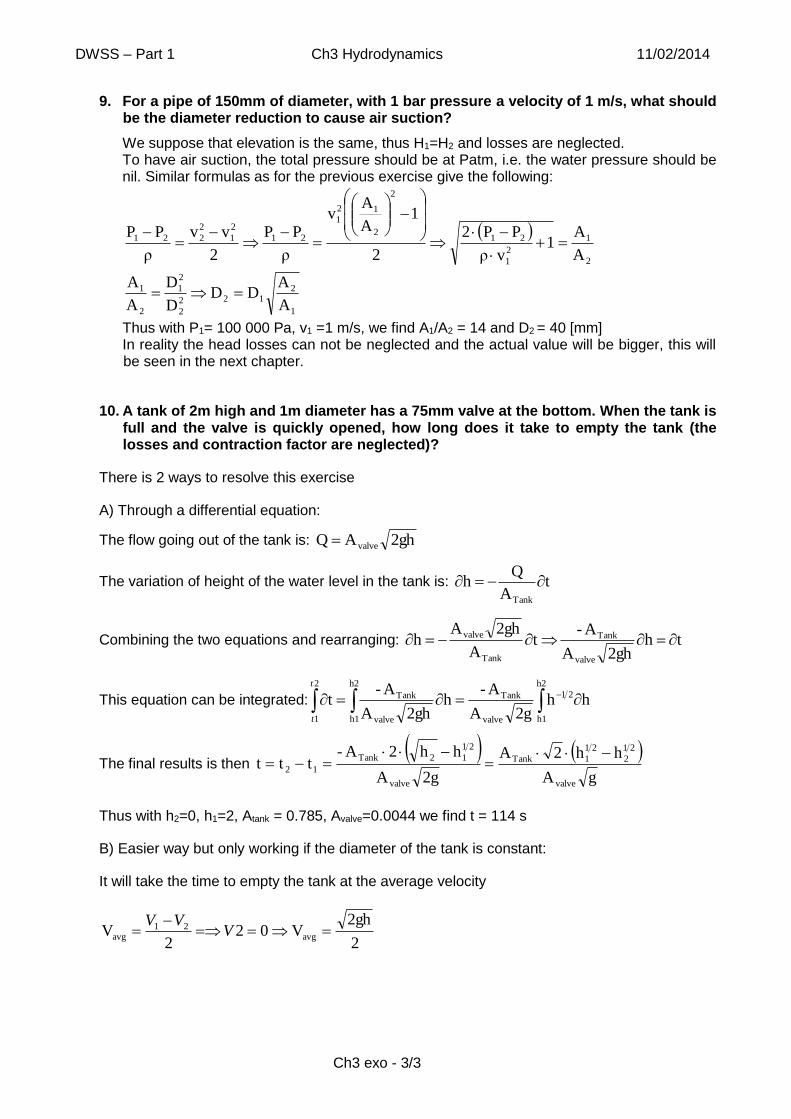
DWSS ndash Part 1 Ch3 Hydrodynamics 11022014
Ch3 exo - 33
9 For a pipe of 150mm of diameter with 1 bar pressure a velocity of 1 ms what should be the diameter reduction to cause air suction
We suppose that elevation is the same thus H1=H2 and losses are neglected To have air suction the total pressure should be at Patm ie the water pressure should be nil Similar formulas as for the previous exercise give the following
2
1
2
1
21
2
2
12
1
21
2
1
2
221
A
A1
vρ
PP2
2
1A
Av
ρ
PP
2
vv
ρ
PP
1
2122
2
2
1
2
1
A
ADD
D
D
A
A
Thus with P1= 100 000 Pa v1 =1 ms we find A1A2 = 14 and D2 = 40 [mm] In reality the head losses can not be neglected and the actual value will be bigger this will be seen in the next chapter
10 A tank of 2m high and 1m diameter has a 75mm valve at the bottom When the tank is full and the valve is quickly opened how long does it take to empty the tank (the losses and contraction factor are neglected)
There is 2 ways to resolve this exercise
A) Through a differential equation
The flow going out of the tank is 2ghAQ valve
The variation of height of the water level in the tank is tA
Qh
Tank
Combining the two equations and rearranging th2ghA
A-t
A
2ghAh
valve
Tank
Tank
valve
This equation can be integrated
h2
h1
21
valve
Tank
h2
h1 valve
Tank
2
1
hh2gA
A-h
2ghA
A-t
t
t
The final results is then
gA
hh2A
2gA
hh2A-ttt
valve
21
2
21
1Tank
valve
21
12Tank
12
Thus with h2=0 h1=2 Atank = 0785 Avalve=00044 we find t = 114 s
B) Easier way but only working if the diameter of the tank is constant
It will take the time to empty the tank at the average velocity
2
2ghV02
2V avg
21avg
V
VV
DWSS ndash Part 1 Ch4 Flow in pipes under pressure 11022014
Ch4 ndash Exo 15
Answers to basic exercises
1 What are the ID the SDR and the Series of a pipe with an outside diameter of 110 mm and a thickness of 66 mm
Using OD = 110 mm and e = 66mm From Eq 4-2 ID = OD ndash 2e ID = 110 - 2 times 66 ID = 968 mm From Eq 4-3 SDR = OD e SDR = 110 66 SDR = 1667 rounded to 17 From Eq 44 S = (SDR-1)2 S = ((11066) -1)2 S = 783 rounded to 8
2 What is the nominal pressure of this pipe if it is made with PVC and used at a temperature of 30degc If it is made with PE80 PE100 at 20degC
From Eq 45 PN = 10 MRS (S C) For a diameter 110 in PVC MRS = 25 MPa and C=2 For temperature lower that 25 degC PN = 10 (25 (8times2) PN = 16 bar But 30degC the derating temperature factor (ft) is = 088 So finally PN is only 14 bar
For a diameter 110 in PE 80 at 20degC MRS = 8 and C= 125 (no derating factor) From Eq 45 PN = 10 times 8 (8 times 125) PN = 8 bar
For a diameter 110 in PE 100 at 20degc MRS = 10 and C= 125 (no derating factor) From Eq 45 PN = 10 times 10 (8 times 125) PN = 10 bar
3 What is the nominal pressure of these PE pipes if it is used for gas (the service ratio is 2 for gas)
For a diameter 110 in PE 80 at 20degc MRS = 8 and C= 2 (no derating factor) From Eq 45 PN = 10 times 8 (8 times 2) PN = 5 bar
For a diameter 110 in PE 100 at 20degc MRS = 10 and C= 2 (no derating factor) From Eq 45 PN = 10 times 10 (8 times 2) PN = 6 bar
4 What are the friction losses in a DN150 PVC pipe of 22 km with a velocity of 1 ms Same question for a cast iron pipe (k=012mm) (can be estimated with figures either log scale of charts in annexes)
PVC pipe
With the charts (taking the chart for k=0005) for a pipe of diameter 150mm and a velocity of 1 ms the result is 056 m100m Given that we have a pipe 22 km long HL= 056 times 22 =123 m
Steel pipe
With the charts (taking the chart for k=012) for a pipe of diameter 150mm and a velocity of 1 ms the result is 07 m100m Given that we have a pipe 22 km long HL= 07 times 22 =154 m
Answers to intermediary exercises
5 What is the hydraulic diameter of a square pipe (b=h) Of a flatten (elliptic) pipe with b=2h
For the square pipe From Eq 47 A = h2 and P = 4h so in Eq 46 Dh = 4 AP Dh= h
For the flatten pipe From Eq 48 A = π h2 2 and P = 3 π h 2 so Dh = 4 AP Dh = 4h 3
6 What is the minimum velocity and flow that should flow to avoid air pocket (Re = 10000) in a pipe of DN25 DN200 DN500
DWSS ndash Part 1 Ch4 Flow in pipes under pressure 11022014
Ch4 ndash Exo 25
From Eq = 49 Re = D middot v ν so v =Re middot ν D
When Re = 10000 the minimum velocity is reached When D = 0025 m v = 10000 times 0000001 0025 v = 04 ms The flow will then be Q = π D2 middot v 4 Q= 314 x (0025) 2 x 04 4 Q= 0196 ls
When D = 02 m v = 10000 0000001 02 v = 005 ms The corresponding flow will be 157 ls When D = 05 m v = 10000x 0000001 05 v = 002 ms The corresponding flow will be 392 ls
7 What is the punctual friction losses coefficient for a pipe connected between to tanks with four round elbows (d=D) a gate valve a non-return valve and a filter
4 round elbows (d=D) Kp = 4 times 035
1 gate valve Kp = 035
1 non-return valve Kp = 25
1 filter Kp = 28
1 inlet Kp = 05
1 discharge Kp = 15 The punctual friction losses coefficient is the sum Kptotal = 905
8 What is the average punctual friction losses coefficient for the accessories of a DN200 pump
A classical setup includes the following items
foot valve with strainer Kp = 15
3 round elbows (d=D) Kp = 3 times 035
1 reduction (dD=08 45deg) Kp = 015
1 extension (dD=08 45deg) Kp = 01
1 gate valve Kp = 035
1 non-return valve Kp = 25 The punctual friction losses coefficient is the sum Kptotal asymp 20 three quarter are due to the foot valve this is usually the most critical part
9 What are the friction losses in a DN150 PVC pipe of 22 km with a velocity of 1 ms Same question for a steel pipe (k=1mm) (to be calculated with equations not estimated with charts)
The Reynolds number is Re = Dmiddotvν Re = 150000
For a PVC pipe the flow will be turbulent smooth From Eq 418 λ = 0309 (log (Re7))2 = 00165 From Eq 415 and kL = λ LD= 00165 times 2 200015 = 2416 From Eq 410 and HL= kLv22g = 123 m
If we compare this result with the one obtained in exercise 4 we see that the results match approximately However the method used in exercise 4 are usually less precise For a DN 150 steel pipe the flow will be turbulent partially rough The ratio kD = 1150 = 0007 From Eq 417 λ = 00055+015(Dk)(13) = 0033 with Eq 419 λ = 0034 thus taking rough instead
of partially rough underestimate the losses From Eq 415 and kL = λ LD= 0034 times 2 200015 = 498 From Eq 410 and HL= kLv22g = 254 m
10 What should be the diameter of an orifice to create losses of 20 meters in a DN100 pipe with a velocity of 1 ms
For an orifice we can use Eq 4-14 K p-o = H P Orifice middot 2g v1
2
with H P Orifice = 20 m and v1 = 1ms K p-o = 391 asymp 400
DWSS ndash Part 1 Ch4 Flow in pipes under pressure 11022014
Ch4 ndash Exo 35
On the chart dD is - if it is a sharp orifice dD = 028 which make d = 28 cm - if it is a beweled orifice dD = 027 which makes d= 27 cm - if it is a rounded orifice dD = 024 which makes d= 24 cm Practically a hole of 24 cm should be done in plate placed between two flanges This orifice can then be filed down to be increased if necessary
Answers to advanced exercises
11 What is the flow in a DN150 galvanised pipe of 800 m connecting two tanks with a gate valve five elbows and a filter if the difference of height between the tanks is 2m 5m 10m
From Eq 4-11 we have HA ndash HB = ∆H = (Q2 ( Kp + Kl) ) (121timesD4)
with D = 015 =gt Q2 = ∆H times 000613 (Kp + Kl) To calculate Kponctual it is necessary to sum all punctual losses the system is composed of
System Kp
1 inlet 05
1 gate valve 035
5 elbows (round) 175
1 filter 28
1 discharge 15
Total Kponctual = 69
To estimate Klinear we calculate the ratio kD = 0001 (D = 150mm and k = 015 m) We can see
in the Moody chart that with this ratio we have a λ between 004 and 002 according to the
Reynolds Let assume a value of 002 (Re gt 800000 turbulent rough) to start Then from Eq 4-15 Klinear = λ LD = 002times800015 = 1067
Then we can calculate the flow Q2 = 2 times 000613 1136 =gt Q= 00104 m3s or 104 ls
The velocity and Reynolds can now be calculated v = 4 middot Q (π times D2) = 059 ms and Re = D middot v ν = 88000
By checking the Moody chart we can see that the λ has roughly a value of 0023 giving a
value of Klinear = 1227 what is not negligible The calculation should be done again with this new value giving Q= 00097 m3s or 97 ls v=055 ms and Re = 83000
This time the Re is close enough to our estimation one iteration was enough to find a precise value
For ∆H = 5m with a λ= 002 we find with the first calculation
Q= 00164 m3s or 164 ls v=093 ms and Re = 140000
For a Re of 140000 lets take a λ=0022 and recalculate Q= 00157 m3s or 157 ls v=089 ms and Re = 133000 what is precise enough
For ∆H = 10m with a λ= 002 we find with the first calculation
Q= 00232 m3s or 232 ls v=131 ms and Re = 197000
For a Re of 197000 lets take a λ=0021 and recalculate
DWSS ndash Part 1 Ch4 Flow in pipes under pressure 11022014
Ch4 ndash Exo 45
Q= 00227 m3s or 227 ls v=128 ms and Re = 192000 what is precise enough
12 How much shall a pipe be crushed to reduce the flow by half
With equation 4-11 we know that 4
LP2
LPBAD
k
121
QHH-H (1)
Given that HA-HB is constant we have 4
1
LP
2
1
D
k
121
2)(Q= 4
2
LP
2
2
D
k
121
)(Q (2)
We assume that λ does not vary significantly with the change occurring after the crushing Furthermore we have kLP = λmiddotLD (3) Putting (3) into (2) and multiplying both sides by 121 we get
5
1
2
1
D
Lλ
4
Q5
2
2
2D
LQ
(4) Which gives us 5
1D
1
5
2D
4 (5) so at the end
75804
1
D
D51
2
1
(6) It is important to notice that while D1 is the nominal diameter D2 is
the hydraulic diameter Dh (since it is an ellipse) Therefore for the rest of the exercise DN and Dh will be used for D1 and D2 respectively Now we want to find h as a function of D For an ellipse (the conduct is crushed in an ellipsoidal shape) we have (eq 4-7)
hb4
πA (7) and NDπh)(b
2
πP (8) because the perimeter of the conduct does not
change if the pipe is crushed From this it follows that ND2hb or hD2b N (9)
substituting (9) into (7) we get
2
N h4
πhD
2
πA (10)
Using equation 4-6 we know that 4
PDA h (11) where Dh is in this case D2 or Dh=0758DN
(12) Substituting (8) and (12) into (11) we get 4
DπD0758A NN (13)
Given that (13)=(10) we get h4
πhD
2
πN =
4
DπD0758 NN (14)
Dividing (14) by π and multiplying by 2 we get 2
N
2
N hhD2D0758 which gives us a second grade equation
0D0758hD2h 2
NN
2 (15) solving this equation we have
2
D07584D4D2h
2
N
2
NN (16) or )0492(1Dh N (17) So the two solutions for
h are
N1 D1492h and h2 = 0508middotDN where DN is nominal diameter of the uncrushed pipe These
two solutions correspond to the pipe being crushed horizontally or vertically
13 What is the flow when the pipe is crushed to half of its diameter
It is the same approach as for ex 11 but the other way around
DWSS ndash Part 1 Ch4 Flow in pipes under pressure 11022014
Ch4 ndash Exo 55
If the pipe is crushed to half its diameter the height of the ellipse (h) will be
ND2
1h (1) As before we have hb
4
πA (2) and NDπh)(b
2
πP (3) which
gives us 2
N h4
πhD
2
πA (4) Substituting (1) into (4) we get
2
N
2
N
2
N D16
3D
16D
4A
(5) Knowing from ex 11 that
4
DD
4
PDA Nhh
(6) We
can set that (5) equal (6) So 2
NNh D
16
3
4
DD
(7) It follows that Nh D
4
3D (8) As in
ex 11 we have
5
1
2
1D
LλQ
5
2
2
2D
LλQ
(9) Where D2 is Dh and D1 is DN Substituting (8) into (9)
we have
5
N
5
2
25
N
2
1
D4
3
Lλ
D
Lλ
QQ (10) and it follows that
25
1
2
4
3
Q
Q (11) or
12 Q4870Q (12)
If we compare this result with what we obtained in ex 11 we see that the result we get here fits to what we calculated previously Indeed in ex 11 in order to reduce the flow by half we had to reduce pretty much the diameter by half Here if we reduce the diameter by half we reduce the flow by almost half of it
DWSS ndash Part 1 Ch5 Open flows 11022014
Ch5 ndash Exo 14
Answers to basic exercises
1 What is the hydraulic radius of a square channel with the same width as depth (h=b)
From Eq 5-3 A = bmiddoth = b2 and P = b+2h = 3b From Eq 5-2 Rh = AP = b2 3b Rh = b3
2 What is the hydraulic radius of a half full pipe (h=D2) of a full pipe (h=D)
For a half full pipe (h=D2) α = 180 deg = π rad From Eq 5-4 A= D2 (π ndash sin(π)) 8 = D2 π 8 P = πD2 From Eq 5-2 Rh = AP = D4 For a full pipe (h=D) α = 360 deg = 2 π rad From Eq 5-4 A= D2 (2π ndash sin(2π)) 8 = D2 π 4 P = 2πD2 = πD From Eq 5-2 Rh = AP = D2 π (4 πD) = D4 The hydraulic radius for a half full pipe and a full pipe is the same
3 What is the flow going through a channel 6m wide 1m deep with a slope of 00001 (n=0015)
Q = Amiddotv = bmiddothmiddotv wit b = 6 m and h = 1 m To determine v we have to use Manning equation (Eq 5-9) where Rh = AP= bmiddoth (b+2h) So Rh = 6times1 (6+2times1) = 075 m S = 00001 C = (Rh 16 )n with n =0015 and Rh = 075 C = 6355
So v = C SRh v = 055 ms
Then Q = 6times1times055 Q = 33 m3s
4 What is the depth of water in a channel 6m wide with a slope of 00001 and a flow of 6m3s (n=0015)
Using Manning equation (Eq 5-9) v = Rh23middotS12 n
with v=QA =gt Q = AmiddotRh23middotS12 n
with A= bmiddoth=6h with Rh= (bmiddoth) (b +2h) = 6h(6+2h)=3h(3+h) Q=bmiddothmiddot(bmiddoth(b+2h))23middot(S)12 n Thus with b=6 we have Q=6hmiddot(3h(1+h))23middot(00001)12 0015 and are looking to solve this equation to find the value of h for Q=6 m3s but it is too complicate to be solved Therefore trial iteration will be done to try to find it With h=1 m depth the flow is Q = 33 m3s flow is too small thus h should be bigger With h=2 m depth the flow is Q = 903 m3s already too high thus the solution is in between With h=15 m depth the flow is Q = 6 m3s the solution is found
5 What is the width of a rectangular channel to carry 135m3s with a 18m water depth and a slope of 00004 (n=0012)
Here the exercise is similar as the previous one but we search the width of the channel with the new parameters for slope n and depth using the same equation as in the previous exercise Q=bmiddothmiddot(bmiddoth(b+2h))23middot(S)12 n with the new values we have Q=18bmiddot(18b(b+36))23middot(00004)12 0012
With b=4 m width the flow is Q = 116 m3s thus to have a bigger flow is should be wider With b=5 m width the flow is Q = 155 m3s the flow is too big thus the solution is in between With b=45 m width the flow is Q = 135 m3s the solution is found
DWSS ndash Part 1 Ch5 Open flows 11022014
Ch5 ndash Exo 24
Answers to intermediary exercises
6 What is the minimum flow to have in a channel 6m wide and 15m water depth to be sure that the flow is turbulent
For a turbulent flow Re gt 10 000 From Eq 5-1 Re = 4 Rhmiddotv ν
The channel is 6 m wide and 15 m high Rh = bmiddoth (b+2h) = 1
So v gt Remiddotν (4Rh) as Q = bmiddothmiddotv Q gt Remiddotνmiddotbmiddoth (4Rh) = Remiddotν(b+2h)4= 104times10-6times9 4
To have a turbulent flow Q must be superior to 00225 m3s or 225 ls
7 A cylindrical pipe with a slope of 0002 should carry 230m3s we want it to be 80 filled What should be the diameter (to be done with the equations)
If the pipe is 80 filled it means that the height h is equal to 80 of the diameter D According to Eq 5-4 α = 2 arcCos ( 1- 2 hD) = 2 arcCos (-06) = 443 Using Eq 5-2 Rh = AP= D (α ndash sin α) 4 α Then as Q = A middot v we can work by iterative approximation to solve 8Q n = (α- Sin α)middot Dmiddot (D (α ndash sin α) 4 α) 23 middot S frac12 As this equation cannot be solved easily it should be done by iteration or by using the Goal Seekhellip function in Excel For Q = 23 m3s S = 0002 n= 00106 and α corresponding to 80 filling the Diameter of the pipe should be 124 m
8 What are the velocity and the height in a DN100 pipe with a flow of 20ls and a slope of 40 (to be done with the fig 5-1 amp 5-2)
Using fig 5-1 we can read for a DN100 at a slope of 40 the flow of the full pipe Qf=40 ls and the velocity is about vf = 51 ms As we have a flow of 20 ls Q = Q Qf = 20 40 = 50 Using fig 5-2 we can read h = 50 thus h = 100 times 05 = 50 mm v = 100 thus v = v middot vf = 51 ms
9 What is the maximum acceptable slope for a smooth DN100 pipe with a flow of 10 ls if we want to limit the velocity at 3 ms at 5 ms (to be done with the fig 5-1 amp 5-3)
Using fig 5-1 we can read for a DN100 with a flow of 10ls the slope of the full pipe Sf=25 and the velocity is about vf = 125 ms As we want a maximum velocity of 3 ms vx = vmax vf = 3 125 = 24 Using fig 5-3 we can read Sx = 6 thus Smax = Sf middot Sx = 25 times 6 = 15 Using fig 5-3 we can read h = 44 thus h = 100 times 044 = 44 mm The maximum admissible slope for this pipe if we want to limit the water velocity at 3 ms is of 15 with a height of 44 mm For a limitation of 5 ms the first step is the same then we have As we want a maximum velocity of 5 ms vx = vmax vf = 5 125 = 4 Using fig 5-3 we can read Sx = 25 thus Smax = Sf middot Sx = 25 times 25 = 625 Using fig 5-3 we can read h = 30 thus h = 100 times 03 = 30 mm The maximum admissible slope for this pipe if we want to limit the water velocity at 5 ms is of 625 with a height of 30 mm
DWSS ndash Part 1 Ch5 Open flows 11022014
Ch5 ndash Exo 34
10 What is the flow going through a V notch weir of 60deg with the height of water of 10cm
If we consider a turbulent flow c=04 and h=01m then Using Eq 5-10 Q = 4 5 times 04 times tg(60deg2) times radic(2 times 981) times (01) 52 = 000259 m3s = 259 ls The value is confirmed by the figure 5-4 The hypothesis on the flow can be confirmed by calculating the Re number From Eq 5-1 Re = 4middotRhmiddotv ν Rh = AP and Q=Av So Re = 4Q νP From trigonometry P=2h cos(θ2) thus Re = 2 times 000259 times cos(602) 01 times 106
so Re = 44 000 it corresponds to a turbulent flow
Answers to advanced exercises
11 Show that the best hydraulic section for a rectangular channel is h=b2
For a rectangular channel we have (eq 5-3) hbA (1) and h2bP (2) It follows from
(1) and (2) that h 2h
AP (3)
We want to minimize the wetted perimeter (P) for a given area (A) In other word we have to derivate P as a function of h and set this to zero to find the minimum
02h
A
h
P2
(4) This gives 2
h
A2 (5) Substituting (1) into (5) we get 2
h
hb2
(6) or
2
bh
12 Knowing that the best hydraulic section for a trapezoidal section is a half hexagon calculate b a and h for a trapezoidal channel having an area of 4m2
Using eq 5-5 we know that ha)(bA (1)
Given that our trapezoid is a half hexagon we can deduct that α is an angle of 60deg (the internal angles in a regular hexagon are of 120deg) We also know that the bottom width (b) equals the side length
Therefore using trigonometric formulas b)cos(60 a (2)
and b)sin(60h (3)
Substituting (2) and (3) into (1) we get
bsin(60)cos(60))bb(A (4) From there we find
m7541)sin(60)1)60(cos(
Ab
(5)
Then from (2) and (5) we find
m0877b)cos(60a
and from (3) and (5) we find
m1520bsin(60)h
b
b h
a
DWSS ndash Part 1 Ch5 Open flows 11022014
Ch5 ndash Exo 44
13 What is the flow going through a rectangular weir of 2m width with a crest height of 1 m and a height of water of 50cm We use eq 5-11 and 5-12
52hg2LcQ (1)
where L = 2 [m] h = 05 [m] z = 1 [m]
4340
105
05501
16051000
11041
zh
h501
16h1000
11041c
22
So sm679050819220434Q 325
DWSS ndash Part 1 Ch6 Pumps 11022014
Ch6 ndash Exo 114
Answers to basic exercises
1 For a pump of 50 m3h at 40 m head (NSasymp20) what is the expected hydraulic power pump efficiency mechanical power motor efficiency and power factor active and total electrical power
Hydraulic power Phydro=ρmiddotgmiddothmiddotQ
water density ρ=1 000 kgm3
gravitational constant g=981 ms2
manometric head h=40m
flow s00139m3600sh
h50mQ 3
3
So Phydro=1000times981times40times00139=5 450 W=545kW Pump efficiency ηp with figure 6-2 (efficiency of centrifugal pumps) for a NS of 20 and a flow of 50 m3h (yellow line) we get an efficiency of 73 Mechanical power Pmec=Phydroηpump=5 450073=7 466 W=747 kW Motor efficiency ηm with figure 6-1 (motor efficiency) For a rated power of approximately 75 kW and a 2-pole motor we get a motor efficiency of 093 Power factor with the same figure but the pink line we get a motor factor of 0895
Total power 897kW W89740730930895
00139409811000
ηηPF
QhgρS
pm
Active power Pelec=SmiddotPF=89737times0895=8032 W = 8 kW
2 What are the nominal head flow efficiency NPSH and power for the pumps a b and c
The nominal head and flow are the one corresponding to the highest efficiency Therefore
DWSS ndash Part 1 Ch6 Pumps 11022014
Ch6 ndash Exo 214
Pump a Pump b Pump c
Head h 63 m 14 m 65 m
Flow Q 100 m3h 375 m3h 2 200 m3s
Efficiency η 76 89 86
NPSH 6 m 3 m 7m
Power P 23 kW 155 kW 48 kW
3 What are the expected minimum and maximum flow for the pumps a b and c
The minimum flow corresponds to the functioning limit point (when the HQ diagram makes a kind of bump) For the maximum flow it is approximately when the lines on the charts end
Pump a Pump b Pump c
Minimum flow Qmin 20 m3h 200 m3h 1500 m3h
Maximum flow Qmax 140 m3h 500 m3h 2500 m3h
4 For the following system what will be the duty point with the pump a what is the power consumption
Elevation 200 masl
Temperature 20degc
All pipes are of new GI DN 175
Total punctual friction losses
- kp = 15 for the suction part
- kp= 5 for the delivery part
1) Estimate the flow
As the pump is already selected we can use its nominal flow for the first estimation (ie Q1 = 100 m3h)
2) Calculate hLP
hLP=punctual losses+linear losses= Lp
2
kk2g
v where
v=QA where s0027m3600sh
h100mQ 3
3
therefore for the first iteration
115ms
0175π4
1
0027
Dπ4
1
Qv
22
15m
215m
1 800 m 100 m 5m
DWSS ndash Part 1 Ch6 Pumps 11022014
Ch6 ndash Exo 314
kp=15+5=20
kL will depend on the velocity but we can either use the chart in the annexes (head losses for pipe under pressure) or use equations 4-15 and 4-19
D
Lλk L where lamda is calculated using eq 4-19
To use eq 419 we need the Reynolds number
102012101
0175115
ν
DvRe
6
which allows us to calculate λ=0020
L is the length of all the pipes L=5+15+100+215+1800=1928 m
D is the diameter 0175m
52181750
19280200kL with equation 4-15 and 4-19
1621m2185209812
115)k(k
2g
vh
2
Lp
2
LP
3) Calculate the total head
3921m1621m15)215(hhh lossesstatictot
4) Find a new Q (Q2)
Looking back in the HQ chart the flow corresponding to a head of 392m is 150 m3h To find this value it is necessary to extrapolate the right hand-side of the chart by extending the end of the curve This is shown in the following chart The purple line is the QP curve given and the blue line is the network curve which can be calculated as explained previously as a function of the flow
5) Iterate
For the next iteration we will take the average between the flow with which we started our calculations (Q1 100 m3h) and the flow we obtained at the end (Q2 150 m3h) which gives us a flow of 125 m3h
The iteration are shown in the following table At the end we find a flow of 130 m3h
90
40
50
60
70
80
20
30
Head h
(m
)
120 140 160 80 100 60 40 20 Q1 Q2 Qduty
DWSS ndash Part 1 Ch6 Pumps 11022014
Ch6 ndash Exo 414
it Q1 m3h Q m3s v Re lamda kL stat
head linear loss
punctual loss
total loss h tot
Q2 m3h
0 100 0028 115 202 101 0019 83 2185 23 1485 136 1621 3921 150
1 125 0035 144 252 626 0019 52 2151 23 2285 212 2497 4797 135
2 130 0036 150 262 732 0019 48 2146 23 2465 230 2695 4995 130
In order to find the corresponding power consumption we look in the QP chart and find a power consumption of 26kW
Answers to intermediary exercises
5 What is the number of poles and the slip value of the motor for the pumps a b and c
For this question we use Eq 6-5 and the corresponding table The number of rotation per minute (n) is written on the very top of each graph series for each pump We then look in the table to find the frequency and number of poles to which it corresponds The number n in the table might not correspond exactly to the number of the n indicated on the graph as the slip value varies from one motor to another After that we have only one unknown in eq 6-5 which becomes solvable
slip
nbPoles
f260n Therefore n-
nbPoles
f260slip
a) The number n=2 900 corresponds to 50 Hz and 2 poles
RPM10029002
50260slip
b) The number n=1 450 corresponds to 50 Hz and 4 poles
RPM5014504
50260slip
c) The number n=980 corresponds to 50 Hz and 6 poles
RPM209806
50260slip
6 What is the specific speed for the pumps a b and c
We use Eq 6-6 where Q and h are the nominal flows and heads found in 2
a)
2363
36001002900
h
QnN
750
50
075
05
s
This Ns correspond to a high head impeller described in the section about specific speed
DWSS ndash Part 1 Ch6 Pumps 11022014
Ch6 ndash Exo 514
The HQ chart has a curve rather flat
The efficiency curve is rounded The power consumption increases as the flow increases
b)
6514
36003751450
h
QnN
750
50
075
05
s
In this case we have a low head impeller
The HQ chart has a steeper curve with a functioning limit point Therefore the functioning range of this pump is smaller than the one used in a
The efficiency curve is less rounded than the one in a (more pointed at the top)
The power consumption is not linear but in overall decreases when the flow increases
c)
18856
36002200980
h
QnN
750
50
075
05
s
In this case we have an axial flow impeller
The HQ chart is even steeper curve with a functioning limit point The functioning range of this pump is very small for this kind of pumps
The efficiency curve is more pointed
The power consumption is not linear but in overall decreases when the flow increases The average slope of this line is steeper than the one in b
7 If we want to adjust the working point of the pump used in exercise 4 to the nominal point with a throttling system what should be the size of the orifice what would be the power consumption
The best efficiency (nominal point) of this pump is for a flow of 100 m3h and a head of 65m Given that for a flow of 100 m3h the head losses are 162 m (first iteration of exercise 4) and the static head stays at 23m the head losses that the orifice will have to create are
hp-orifice=63m-23m-162m=238m
DWSS ndash Part 1 Ch6 Pumps 11022014
Ch6 ndash Exo 614
With eq 4-14 we have
2g
vkh
2
oporifice-p where v is the velocity corresponding to a flow of 100m3h
1155
0175π4
1
1003600
Dπ4
1
Qv
22
ms (again this velocity can be read from the first
iteration exercise 4)
Therefore 0531155
9812238
v
2ghk
22
orifice-p
op
Therefore if we choose a sharp orifice we find (with the losses due to orifice chart in chapter 4) a dD ratio of 029 Given that our D=175mm d=029times175=51mm (which is the diameter of the orifice the edge of the orifice being sharp)
The power consumption will then be (looking in HP chart) of 23kW
This corresponds to a reduction of 13 compared to the system as it is working in exercise 4
8 With the same situation as exercise 4 what would be the new flow and power consumption if we decrease the rotation speed so that it reaches 80 of its initial value
The first thing is to define a new HQ curve For this we calculate the flow and the head at minimal maximal and optimal points
1
1
212 08Q
n
nQQ
1
2
1
212 064h
n
nhh
Therefore
90
40
50
60
70
80
20
30
Head h
(m
)
120 140 160 80 100 60 40 20
Static head
Head losses wo orifice
Head losses due to orifice
system curve with orrifice
system curve without orrifice
pump characteristic curve
DWSS ndash Part 1 Ch6 Pumps 11022014
Ch6 ndash Exo 714
100 80 100 80
Qmin 20 m3h 16 m3h hmax 80 m 52 m
Qopt 100 m3h 80 m3h hopt 63 m 40 m
Qmax 140 m3h 112 m3h hmin 45 m 29 m
The HQ curve will look like the one given but shifted to the bottom and right Knowing that we can draw the HQ curve of the pump It looks like that
Next we do the same as with point 4 with this new HQ curve
1) Estimate the flow
We take the nominal flow ie Q1=80 m3h
2) Calculate hLP
HLP=punctual losses+linear losses= Lp
2
kk2g
v where
092ms
0175π4
1
803600
Dπ4
1
Qv
22
kp=15+5=20
D
Lλk L where lamda is calculated using eq 4-19
681161101
0175092
ν
DvRe
6
which allows us to calculate λ=0020
L is (as for point 4) 1928 m and D is 0175m
52221750
19280200kL with equation 4-15 and 4-19
m55102225209812
092)k(k
2g
vh
2
Lp
2
LP
3) Calculate the total head
335mm51015)215(hhh lossesstatictot
50
60
70
30
40
Head h
(m
)
120 140 160 80 100 60 40 20
80
Qmin Qopt Qmax
hmin
hopt
hmax
DWSS ndash Part 1 Ch6 Pumps 11022014
Ch6 ndash Exo 814
4) Find a new Q (Q2)
Looking back at the pump characteristics the flow corresponding to a head of 335m is 105m3h This is shown in the following chart As before the purple line is the QP curve given and the blue line is the network characteristics which is the same as the one drawn in point 4
5) Iterate
The average between Q1 (80 m3h) and the flow we obtained at the end Q2 (105 m3h) which gives us a flow of 925 m3h
The iteration are shown in the following table At the end we find a flow of 95 m3h
it Q1 m3h Q m3s v Re lamda kL
stat head
linear loss
Punctual loss
total loss h tot
Q2 m3h
0 80 0022 092 1616812 0020 22250 23 968 087 1055 3355 105
1 925 0026 107 1869439 0020 21984 23 1279 116 1395 3695 97
2 9475 0026 109 1914912 0020 21942 23 1339 122 1461 3761 96
For the power consumption knowing that the flow is 95 m3h and that the power consumption
for this flow is 22 kW we will have 113kW0822n
nPP
3
3
1
212
As it can be noticed the power consumption passes from 26 kW without adjustment to 23kW with a throttling system and to 113 kW with a speed reduction system Compared with a throttling system (where we have almost the same flow reduction) the power consumption with a speed decrease system is much more efficient
9 If the system is working as per exercise 4 what is the maximum suction height And what is the maximum suction height if it is working as in exercise 7
The maximum suction head is when it is equal to the height of the water column minus the head losses in the suction part and the NPSH required by the pump
rS-LPva
suc NPSHhgρ
PPh
At 200 masl the atmospheric pressure is 98 000 Pa (chart chapter 2 page 3) In this exercise we want to avoid cavitation Therefore we have to take the minimum pressure on the chart (light blue line) representing the smallest water column The vapour pressure for water at 20degC is 2340 Pa (figure 2-3)
The height of the water column is mg
PP va 7599811000
234098000
The head losses in the suction part are calculated as follow
40
50
60
20
30
Head H
(m
)
120 140 160 80 100 60 40 20
Q1 Q2 Qduty
DWSS ndash Part 1 Ch6 Pumps 11022014
Ch6 ndash Exo 914
Lp
2
LP kk2g
vh where v=QA and kp=15 (punctual losses in the suction part)
The NPSHr is given in the chart NPSH versus flow
a) When the system is working as per exercise 4
The flow for this system is 130 m3h
The height of the water column is 975m
The head losses in the suction part we have
- kp for the suction part that is 15
- 11850175
10650019
D
LλkL where lambda is from the last iteration of point 6
L=5+15+100=1065 and D is the diameter 0175m
m0831185)(159812
51kk
2g
vh
2
Lp
2
LP
The NPSH For a flow of 130 m3h we find a NPSH of 8 m
Therefore the maximum is 133m8308759hsuc this negative number indicates
clearly that the system designed in point 6 only works if the pump is placed at least 135m below the water level If not cavitation will occur will damage the pump and reduce the flow
b) When the system is working as per exercise 7 (adjustment with a throttling system)
The height of the water column stays at 975m
The head losses in the suction part we have
- kp = 15 for the suction part
- 12070175
10650020
D
LλkL where lamda was recalculated for this flow with eq
419
189m)0712(159812
171kk
2g
vh
2
Lp
2
LP
The NPSH For a flow of 100 m3h we find a NPSH of 6 m
Therefore the maximum is 186m6189759h suc This value being higher than 15 m
(which is the suction height of the pump as it is designed in point 6) indicates that cavitation will not occur with this system
The maximum suction height between point a and b is increased because the flow is decreased which will decrease the head losses and the NPSH required by the pump Thus if we want this system to work without cavitation the flow has to be reduced by throttling trimming or speed reduction
DWSS ndash Part 1 Ch6 Pumps 11022014
Ch6 ndash Exo 1014
Answers to advanced exercises
10 For the system used in exercise 7 (with a throttling system) knowing that the intake water level varies of plus or minus 2 meters what would be the max and min flow what would be the max suction height
a) With plus 2 meters
The flow
We have to do the same iterations as it was done in exercise 4 This time the static head is 21m instead of 23m We can begin the iteration at 100 m3h since the flow will be practically the same (the static head does not change much)
The punctual losses coefficient is equal to the punctual losses in the suction part and delivery part plus the one of the orifice kp=15+5+350=370
it Q
m3h Q
m3s V
ms Re lamba kL
H static
Linear losses
Punctual losses
Total loss h tot
Q2 m3h
0 100 0028 115 2021015 0020 21851 21 1485 2515 4001 6101 1048
1 1024 0028 118 2069280 0020 21813 21 1554 2637 4191 6291 998
2 1011 0028 117 2043199 0020 21833 21 1517 2571 4088 6188 1025
3 1018 0028 118 2057735 0020 21822 21 1538 2607 4145 6245 1010
Thus by decreasing the static head the flow is increased of about 1 Q= 101 m3h
The maximum suction height (for this water level) is calculated as in exercise 9
o the height of the water column is 975 m
o the head losses in the suction part are
921)1750
51060200(15
9812
181
D
Lk
2g
vh
2
p
2
LP
m
o the NPSH is around 6m for a flow of 101 m3h
Therefore the maximum suction height is 975m-192m-6m=184
It must be noticed that it is 184m above the water level for which we calculated the flow which is 2 meters above the average suction level Therefore when the water level is 2m above the
hstat
Minus two meter b
Plus two meters a Average suction level
90
40
50
60
70
80
20
30
Head H
(m
)
120 140 160 80 100 60 40 20 Qa Qb
DWSS ndash Part 1 Ch6 Pumps 11022014
Ch6 ndash Exo 1114
average water level the pump should be placed at a maximum of 384m above the average water level
b) with minus 2 meters
The flow
We have to do the same iterations as it was done before This time the static head is 25m instead of 23m Again we start at a flow of 100 m3h
it Q m3h Q m3s v Re lamda kL
stat head linear loss
punctual loss total loss h tot Q2
0 1000 0028 115 2021015 0020 21851 25 1485 2515 4001 6501 941
1 970 0027 112 1960891 0020 21902 25 1402 2368 3769 6269 1004
2 987 0027 114 1994890 0020 21873 25 1449 2451 3899 6399 969
3 978 0027 113 1976407 0020 21888 25 1423 2405 3828 6328 988
4 983 0027 114 1986684 0020 21880 25 1437 2430 3868 6368 977
5 980 0027 113 1981039 0020 21884 25 1429 2417 3846 6346 983
(The number of iterations necessary to converge on the result has increased because the system curve is steeper which makes the iteration process less efficient)
This time by increasing the static head the flow is decreased of about 2 Q= 98 m3h
The maximum suction height (for this water level) is calculated as before
o the height of the water column is 975 m
o the head losses in the suction part are
m781)1750
51060200(15
9812
131
D
Lk
2g
vh
2
p
2
LP
o the NPSH is around 6m for a flow of 98 m3h
Therefore the maximum suction height is 975m-178m-6m=197m
This height corresponds to a height of 197m above the water level for which we calculated the flow (which is 2 meters below the average suction level) Therefore the pump should be placed just below the average water level or lower (2m-197m=003m=3cm) This level is (not surprisingly) lower than the one obtained in a Therefore this is the value to be considered when doing the design to find the elevation of the pump avoiding cavitation As a result if the pump is place 15 m above the surface level (as it is the case in exercise 7) it will cavitate when the water level will drop down As it can be seen the variation of the water level in the intake tank has a big impact on cavitation and should be taken into account when doing calculations
11 With a frequency inverter what should be the percent speed reduction to adjust the system to the nominal point of the pump What is the corresponding flow
As it is explained in the section about speed reduction the line of nominal points with a speed reduction is parable In order to find the point where the system is at its nominal point we will have to find the place where the nominal point line crosses the system curve This is shown on the following graph
DWSS ndash Part 1 Ch6 Pumps 11022014
Ch6 ndash Exo 1214
0
20
40
60
80
100
120
140
0 50 100 150
Flow (m3h)
Head
(m
)
System curve
Line of nominal point
Pump curve w ithout speed
reduction
Pump curve w ith x speed
reduction
First we have to find the equation of this parable A parable is from the type
y=ax2+bx+c In our case it is hn=aQn2+bQn+c (hn and Qn indicates the nominal head and
nominal flow respectively)
We know that it passes by the origin thus c=0 Therefore the equation of the parable will be from the type
hn=aQn2+bQn
To find the coefficient a and b we need two points on this curve
If we do not change the system the nominal point is Qn=100 m3h and hn=63 which will be the first of the two needed points
The second point (which is whichever point on the curve with r rotation speed) will have apostrophe (Hn and Qn) to make the difference between the first (with 100 speed) and second point (r speed)
2
n
n
n
n
n
2
n
n
n
2
nn
rhh(4)
rQQ(3)
QbQah(2)
QbQah(1)
Substituting (3) and (4) into (2) we get
rbQraQrh)5( n
22
n
2
n
which simplifies to (dividing by r)
n
2
nn bQraQrh(6)
From (1) we know that
2
nnn QahQb)7(
Putting (7) back into (6) we get
2
nn
2
nn QahrQarh)8(
DWSS ndash Part 1 Ch6 Pumps 11022014
Ch6 ndash Exo 1314
which can be written as
1)(rQa1)(rh)9( 2
nn
If follows that
2
n
n
Q
ha)10( In that case given that Qn=100 m3h and hn=63 we have 30006
100
63a
2
To find the coefficient b we use (10) and (1) and find
n
2
n2
n
nn QbQ
Q
hh)11(
which gives us b=0
Therefore our equation of the line of nominal point is 200063Qh
To find the intersection of the line of nominal point and the system curve we will have to iterate in a slightly different way as before
For a given flow Q1 we will estimate the losses and the total head (static head plus head losses) as it was done before
Then for this head we will find the corresponding flow Q2 on the line of nominal points To find the nominal flow for a given head we solve the following equation for Q
0h00063Q2 which gives us 00063
hQ
This time Q2 can directly be taken for the next iteration (no need to do the average between Q1 and Q2) This is because between Q1 and Q2 we do not cross the intersection as it was the case for the previous iterations (this can be seen in the following figure) Therefore we get closer to the results every time and Q2 can be taken for the next iteration
We will start the iteration at the nominal flow without speed reduction system namely 100 m3h The iterations are shown in the following table
0
20
40
60
80
100
120
140
0 50 100 150
System curve Line of nominal point
Q1 Q2
DWSS ndash Part 1 Ch6 Pumps 11022014
Ch6 ndash Exo 1414
it Q m3h
Q m3s v Re lamda kL
stat head
linear loss
punctual loss
total loss total h Q2
0 100 0028 115 202102 002 21851 23 148538 13595 162134 3921 789
1 7889 0022 091 159447 002 22277 23 942562 08462 102718 3327 727
2 7267 002 084 146872 002 22441 23 805645 0718 877446 3177 71
3 7102 002 082 143529 002 22489 23 771023 06857 839593 314 706
4 7059 002 082 142671 002 22501 23 762262 06775 830015 313 705
At the end we get approximately a flow of 70 m3h
Given that 1
2
1
2
n
n
Q
Q and that we have 07
100
70
Q
Q
1
2 it follows that 07n
n
1
2
Therefore the speed reduction should be of 70
For the pump a we have a frequency of 50 Hz Given that the rotation speed is directly proportional to the frequency the frequency will have to be reduced to 70 of its initial value which is 35 Hz
DWSS ndash Part 1 Ch7 Water hammer 11022014
Ch7 ndash Exo 17
Answers to basic exercises
1 Draw the pressure and the velocity versus the time (Lc) at the middle of the pipe for an instantaneous valve closure neglecting head losses
The surge will arrive at the middle of the pipe after half of the time needed to travel the pipe L2c and come back after two times this time 2L2c=Lc
2 What are the velocity of the pressure wave (c) the head surge (Δh) and the return time in a cast iron pipe DN200 of 3 kilometres for a instantaneous decrease of velocity of 15 ms
With the table of Cast iron pipe in the annexe N we find with DN200 the value of c=1216 ms To find Δh we have to multiple the given value by the actual velocity Δh=124times15=186 m To find the return time we have to multiple the given value by the actual length in km Tr=16times3=48 s
In this case the pressure surge is huge (almost 18 bar) but the return time very short thus if it is possible to extend the closure or stopping time to 10 s the surge would be divided by 2 (9 bar) and with 20 s by 4 (ie 45 bar)
3 What are the velocity of the pressure wave (c) the head surge (Δh) and the return time in a PE pipe SDR11 of 5 kilometres for a instantaneous decrease of velocity of 2 ms
With the table of PE pipe in the annexe N we find with SDR11 (the diameter of the pipe is not needed the water hammer will be the same for the all series) the value of c=342 ms To find Δh we have to multiple the given value by the actual velocity Δh=35times2=70 m To find the return time we have to multiple the given value by the actual length in km Tr=58times5=29 s
In this case we can see that the pressure surge is smaller (~7 bar) but that the return time is quite important almost half minute before the surge is back
4 What are the velocity of the pressure wave (c) the head surge (Δh) and the return time in a PVC pipe SDR17 OD 200 of 2 kilometres for a instantaneous closure with an initial velocity of 1 ms
With the table of PVC pipe ODgt100 in the annexe N we find with SDR17 (the water hammer will be the same for the all series with ODgt100) the value of c=490 ms The Δh is the one in the table as the velocity is of 1 ms Δh=50 m To find the return time we have to multiple the given value by the actual length in km Tr=41times2=82 s
In this case we can see that the pressure surge is quite small (~5 bar) and the return time not too long (less than 10 s) Thus this pipe should be not too much at risk
pre
ssure
time
L2c
-ΔP
P0
t0 Lc 2Lc 3Lc 4Lc
+Δ
P
1 2
5Lc
3 4 Phases
t0
Reversed flow
Ve
locity
v0
Lc Lc
time Lc 2Lc 3Lc 4Lc 5Lc
DWSS ndash Part 1 Ch7 Water hammer 11022014
Ch7 ndash Exo 27
5 What length of the previous pipe will have a reduced surge if the closure time is of 41 second
The length with reduce surge is according to eq 74 is Lred = Tc c 2 = 41 times 490 2 = 1000 m Thus with a decreasing time of half the return time half of the pipeline will have reduced pressure durge
6 Neglecting losses draw the envelope scheme for the previous pipe knowing that its profile is as per the attached table Is the pipe safe (assuming a linear front wave) If not what can be done
Pump Pt 1 Pt 2 Pt 3 Tank
Pipe length 0 500 1000 1500 2000
Elevation 0 10 30 30 70
We can see that a part of the pipeline (between 750 and 1 200) will be exposed to depressure and that around 1 000 m it might even face cavitation There is no risk of pipe burst (over pressure) as the maximum pressure (hstat + Δh = 120) is smaller than the pipe PN (~125 m) In order to avoid this depressure in the pipe the following could be done - Increase the stopping time - Install air valves letting air come into the pipe in the zone at risk
7 For the previous system what should be the closure time to limit the Δh at 30m
According to Eq 75 s61330819
120002
hg
v2LT
Tg
v2Lh
max
inc
c
inmax
Thus to reduce the Δh to 30 m the closure time should be of 136 s In theory this would be also valid for a cast iron pipe or any material with a return time for this system smaller than 136 s
Δh=50m
Static line
Lred = 1 000 m
Zone at risk
Min acceptable pressure
Max acceptable pressure
Δh=50m
500 1 000 1 500 2 000
70
30
10
120 125
Pipe length [m]
Elevation [m]
-8
DWSS ndash Part 1 Ch7 Water hammer 11022014
Ch7 ndash Exo 37
Answers to intermediary exercises
8 Draw the pressure and the velocity versus the time (Lc) at the middle of the pipe for an instantaneous valve closure taking into consideration head losses
The surge will arrive at the middle of the pipe after half of the time needed to travel the pipe L2c and come back after two times this time 2L2c=Lc
9 What are the velocity (c) the head surge (Δh) and the return time (Tr) of the pressure wave in a cast iron pipe DN200 (e=64 mm Kpipe=140 GPa) of 3 km if a pump of 170 m3h instantaneously stops working with a temperature of water of 45deg
We calculate c with Eq 7-1
pipe
water
water
K
K
e
D1
ρKc
where at 45deg Kwater is 229 GPa and ρ=9902 kgm3
The thickness e is 64 mm KCI is 140 GPa
The diameter D can be estimated as the nominal diameter (DN) so 200 mm
so ms 1237
10140
10229
64
2001
990210229
K
K
e
D1
ρKc
9
9
9
pipe
water
water
Given that the flow is totally stopped
ms 150
102004
π
1703600
A
QvΔv
23
The head surge is found with equation 7-1 Δh = Δvmiddotcg=15 times 1237 981 = 1896 m
The return time is found with equation 7-3 Tr= 2Lc= 2 times 3000 1237 = 485 s
If we compare these results with the exercise 2 we can see that they are very close the difference of taking in to consideration the water temperature of 45deg make a difference of 15 on the head surge and of 1 on the return time
pre
ssure
time
L2c
-ΔP
P0
t0 Lc 2Lc 3Lc 4Lc
+Δ
P
1 2
5Lc
3 4 Phases
t0
Reversed flow
Ve
locity
v0
Lc Lc
time Lc 2Lc 3Lc 4Lc 5Lc
DWSS ndash Part 1 Ch7 Water hammer 11022014
Ch7 ndash Exo 47
10 For the previous pipe we want to limit the head surge at 100m by having a longer stopping time what should be in this case TC
According to equation 7-5 we have s 179100819
5130002
hg
v2LT
max
inc
BY increasing significantly the closure time we will have almost half of the flow when the head surge is coming back therefore the Δv is divided by two dividing thus also the head surge by two
11 What are the velocity (c) the head surge (Δh) and the return time (Tr) of the pressure wave in a PE80 pipe PN125 OD200 (KPE=07 GPa e=182mm) of 5 km if a pump of 150 m3h instantaneously stops working with a temperature of water of 20deg
We calculate c with Eq 7-1
pipe
water
water
K
K
e
D1
ρKc
where at 20deg Kwater is 22 GPa and ρ=9982 kgm3
The nominal thickness for this pipe is given 182 mm (an average of 192 could be used)
The bulk modulus KPE is given as 07 GPa
The internal diameter D is thus per Annexe B 1636 mm
so ms 742
1070
1022
182
16361
99821022
K
K
e
D1
ρKc
9
9
9
pipe
water
water
Given that the flow is totally stopped
ms 1982
102004
π
1503600
A
QvΔv
23
The head surge is found with equation 7-1 Δh = Δvmiddotcg=1982 times 274 981 = 555 m
The return time is found with equation 7-3 Tr= 2Lc= 2 times 5000 274 = 364 s
This time if we compare these results with the exercise 3 we can see that they are not so close as the bulk modulus given is quite different from the one used in the table in annexe N
12 What are the friction coefficient (KLP) and the head losses (hLP) of the previous pipe with a roughness of 007 mm neglecting the punctual losses What is the attenuation of the negative head surge due to the losses at the tank
With equation 4-9 we find Re = D middot v ν = 1636 times 1982 101 times 10-6 = 322 000
With equation 4-19 or fig 4-5 we find λ = 00147
As the singular losses are neglected we find with equations 4-15
KLP = λ middot L D = 00147 times 5 000 01636 = 449
hLP = v2 middot λ 2g = 19822 times 449 (2 times 981) = 899 m
Thus the attenuation of the negative head surge at the tank is equal to hlosses2 about 45m In this situation where the losses are quite high as the velocity is important we can see that the remaining negative head surge at the tank is only of 10m thus the importance to take them in to account
DWSS ndash Part 1 Ch7 Water hammer 11022014
Ch7 ndash Exo 57
13 What are the attenuation of head surge at the valve (hv-att) the remaining velocity at the tank (vt1) and the attenuation of the positive head surge at the tank (ht-att) of the previous pipe
With equation 7-6 we find m 8254499812
7421-274
982144921
2gk
c1-c
vk21
h
2
2
LP
2
2
inLP
att-v
With equation 4-9 we find
m 52494981
7421-274
6071982149412
gk
c1-c
vvk12
h
ms 60712744
9821449
4c
vkv
2
2
LP
2
2
t1inLP
att-t
22
inLPt1
Thus when the surge arrive to the tank the velocity in the depression zone reaches 1607 ms This explains why the negative head surge is so small at the tanks as the difference of velocity is then only of 1982-1602=0375 ms
The attenuation of the positive head surge at the valve is of 258 m thus the positive head surge at the valve is of 555 - 258 asymp 30 m NB this value as to be added at the static level not at the dynamic one This value is much smaller than the initial head losses (899 m) thus the positive head surge is not affecting the pipe at the valve
The attenuation of the positive head surge at the tank is of 25 m thus the positive head surge at the tank is of 555 ndash 899 2 ndash 25 asymp 8 m This remaining positive head surge at the tank is very small
See the next exercise correction for an illustration of these results
14 For the previous pipe draw the developed profile of the pipeline the static and dynamic lines and the envelope schemes knowing that its profile is as per the attached table Is the pipe safe If not what can be done
Pump Pt 1 Pt 2 Pt 3 Tank
Pipe length 0 1000 1000 1000 2000
Elevation 0 0 5 10 30
As explain in the section 76 the developed profile should be used but as the slopes are small it doesnt make a big difference if it is taken into consideration or not
All the values calculated in the previous exercises were reported in this chart
It can be seen that the superior envelope is much lower than the maximum acceptable pressure thus there is no risk of pipe burst in case of water hammer
However the inferior level is lower than the ground level even lower than the cavitation line (minimum acceptable pressure) thus depressure and cavitation will happen in this pipeline if it is not protected
Possible solutions might include a pump bypass system or air valve Nevertheless into this situation the best would be to increase the diameter of the pipe decreasing also the losses and necessary PN for the pipe this will thus decrease the thickness and further the head surge
DWSS ndash Part 1 Ch7 Water hammer 11022014
Ch7 ndash Exo 67
15 What would be the effect on the head surge on the previous exercises of having a Youngs modulus (KPE)of 11 GPa instead of 07 GPa
The surge velocity will be at 341 ms instead of 274 ms increasing the head surge at 70 m instead of 56 m This will significantly increase the problematic of the depressure at the valve even for bigger diameters This shows the importance to have a good information from the supplier about the properties of the pipes and in case of doubt to take a good margin between the envelope and the maximum or minimum tolerable pressure
16 For exercise 2-4 what would be the change in ID (DN for metallic pipe) following the change in pressure due to water hammer
In order to calculate ΔD we use a formula from chapter 1 (Eq 1-5)
2e
D
K
ΔPDΔD
K is the Youngs modulus of the pipe material For the first exercise to find ΔD in mm we have
0026mm642
200
10125
1053400200ΔD
9
Therefore when the pipe will be in overpressure the DN will be Do=200+0026=200026 mm (the pipe will be expanded)
When the pipe will be in under pressure the DN will be Du= 200-0026=19997
Answers to advanced exercises
11m
Developed profile of the pipeline
-30
-10
10
30
50
70
90
110
130
0 500 1000 1500 2000 2500 3000 3500 4000 4500 5000
Dynamic or piezo line
Static line
Overpressure envelope
Depressure envelope
Pipeline
Min acceptable pressure
Max acceptable pressure
0
Elevation
PN
of
the p
ie ~
123m
Head losses
~90m
Attenuated positive head surge at the
valve ~30m
Tank elevation
~30m
Depressure ~56m
Pipe length [m]
Cavitation ~9m Head losses2
~45m
Attenuation of head surge at the valve
~26m Head losses2 +
ht-att ~48m
8m
DWSS ndash Part 1 Ch7 Water hammer 11022014
Ch7 ndash Exo 77
The same procedure is done for exercise 3 amp 4 The results are shown it the following table
Ex ΔP Pa DN or ID mm e mm K GPa ΔD mm Do mm Du mm
2
3
4
We can draw the following conclusion
even if the ΔP is bigger for cast iron the change in diameter will be less than for PE (because PE is easily distorted)
even if the ΔP is bigger for exercise 4 than for 3 the change in pipes diameter will be bigger for 3 because the wall thickness is smaller (which makes the pipe more easily distorted)
It can be noticed that the expansion due to changes in pressure in the pipe is not significant because even for PE pipe with a bigger expansion it is around half a millimetre added to the outside diameter which is less than the tolerance margin for PE pipe For example for a PE pipe having an OD of 200 mm the maximum outside diameter will be of 2012 mm (which is bigger than 2005 obtained with pressure expansion) These calculations were done for expansion due to pressure changes only because of water hammer (thus ignoring the initial pressure in the pipe) This means that the diameter can be more expanded because the total change in pressure will be bigger Furthermore if we have an initial pressure it must be checked that the PN of the pipe can bear the total pressure (initial pressure +ΔP)

DWSS ndash Part 1 Ch4 Flow in pipes under pressure 11022014
Ch4 ndash Exo 55
If the pipe is crushed to half its diameter the height of the ellipse (h) will be
ND2
1h (1) As before we have hb
4
πA (2) and NDπh)(b
2
πP (3) which
gives us 2
N h4
πhD
2
πA (4) Substituting (1) into (4) we get
2
N
2
N
2
N D16
3D
16D
4A
(5) Knowing from ex 11 that
4
DD
4
PDA Nhh
(6) We
can set that (5) equal (6) So 2
NNh D
16
3
4
DD
(7) It follows that Nh D
4
3D (8) As in
ex 11 we have
5
1
2
1D
LλQ
5
2
2
2D
LλQ
(9) Where D2 is Dh and D1 is DN Substituting (8) into (9)
we have
5
N
5
2
25
N
2
1
D4
3
Lλ
D
Lλ
QQ (10) and it follows that
25
1
2
4
3
Q
Q (11) or
12 Q4870Q (12)
If we compare this result with what we obtained in ex 11 we see that the result we get here fits to what we calculated previously Indeed in ex 11 in order to reduce the flow by half we had to reduce pretty much the diameter by half Here if we reduce the diameter by half we reduce the flow by almost half of it
DWSS ndash Part 1 Ch5 Open flows 11022014
Ch5 ndash Exo 14
Answers to basic exercises
1 What is the hydraulic radius of a square channel with the same width as depth (h=b)
From Eq 5-3 A = bmiddoth = b2 and P = b+2h = 3b From Eq 5-2 Rh = AP = b2 3b Rh = b3
2 What is the hydraulic radius of a half full pipe (h=D2) of a full pipe (h=D)
For a half full pipe (h=D2) α = 180 deg = π rad From Eq 5-4 A= D2 (π ndash sin(π)) 8 = D2 π 8 P = πD2 From Eq 5-2 Rh = AP = D4 For a full pipe (h=D) α = 360 deg = 2 π rad From Eq 5-4 A= D2 (2π ndash sin(2π)) 8 = D2 π 4 P = 2πD2 = πD From Eq 5-2 Rh = AP = D2 π (4 πD) = D4 The hydraulic radius for a half full pipe and a full pipe is the same
3 What is the flow going through a channel 6m wide 1m deep with a slope of 00001 (n=0015)
Q = Amiddotv = bmiddothmiddotv wit b = 6 m and h = 1 m To determine v we have to use Manning equation (Eq 5-9) where Rh = AP= bmiddoth (b+2h) So Rh = 6times1 (6+2times1) = 075 m S = 00001 C = (Rh 16 )n with n =0015 and Rh = 075 C = 6355
So v = C SRh v = 055 ms
Then Q = 6times1times055 Q = 33 m3s
4 What is the depth of water in a channel 6m wide with a slope of 00001 and a flow of 6m3s (n=0015)
Using Manning equation (Eq 5-9) v = Rh23middotS12 n
with v=QA =gt Q = AmiddotRh23middotS12 n
with A= bmiddoth=6h with Rh= (bmiddoth) (b +2h) = 6h(6+2h)=3h(3+h) Q=bmiddothmiddot(bmiddoth(b+2h))23middot(S)12 n Thus with b=6 we have Q=6hmiddot(3h(1+h))23middot(00001)12 0015 and are looking to solve this equation to find the value of h for Q=6 m3s but it is too complicate to be solved Therefore trial iteration will be done to try to find it With h=1 m depth the flow is Q = 33 m3s flow is too small thus h should be bigger With h=2 m depth the flow is Q = 903 m3s already too high thus the solution is in between With h=15 m depth the flow is Q = 6 m3s the solution is found
5 What is the width of a rectangular channel to carry 135m3s with a 18m water depth and a slope of 00004 (n=0012)
Here the exercise is similar as the previous one but we search the width of the channel with the new parameters for slope n and depth using the same equation as in the previous exercise Q=bmiddothmiddot(bmiddoth(b+2h))23middot(S)12 n with the new values we have Q=18bmiddot(18b(b+36))23middot(00004)12 0012
With b=4 m width the flow is Q = 116 m3s thus to have a bigger flow is should be wider With b=5 m width the flow is Q = 155 m3s the flow is too big thus the solution is in between With b=45 m width the flow is Q = 135 m3s the solution is found
DWSS ndash Part 1 Ch5 Open flows 11022014
Ch5 ndash Exo 24
Answers to intermediary exercises
6 What is the minimum flow to have in a channel 6m wide and 15m water depth to be sure that the flow is turbulent
For a turbulent flow Re gt 10 000 From Eq 5-1 Re = 4 Rhmiddotv ν
The channel is 6 m wide and 15 m high Rh = bmiddoth (b+2h) = 1
So v gt Remiddotν (4Rh) as Q = bmiddothmiddotv Q gt Remiddotνmiddotbmiddoth (4Rh) = Remiddotν(b+2h)4= 104times10-6times9 4
To have a turbulent flow Q must be superior to 00225 m3s or 225 ls
7 A cylindrical pipe with a slope of 0002 should carry 230m3s we want it to be 80 filled What should be the diameter (to be done with the equations)
If the pipe is 80 filled it means that the height h is equal to 80 of the diameter D According to Eq 5-4 α = 2 arcCos ( 1- 2 hD) = 2 arcCos (-06) = 443 Using Eq 5-2 Rh = AP= D (α ndash sin α) 4 α Then as Q = A middot v we can work by iterative approximation to solve 8Q n = (α- Sin α)middot Dmiddot (D (α ndash sin α) 4 α) 23 middot S frac12 As this equation cannot be solved easily it should be done by iteration or by using the Goal Seekhellip function in Excel For Q = 23 m3s S = 0002 n= 00106 and α corresponding to 80 filling the Diameter of the pipe should be 124 m
8 What are the velocity and the height in a DN100 pipe with a flow of 20ls and a slope of 40 (to be done with the fig 5-1 amp 5-2)
Using fig 5-1 we can read for a DN100 at a slope of 40 the flow of the full pipe Qf=40 ls and the velocity is about vf = 51 ms As we have a flow of 20 ls Q = Q Qf = 20 40 = 50 Using fig 5-2 we can read h = 50 thus h = 100 times 05 = 50 mm v = 100 thus v = v middot vf = 51 ms
9 What is the maximum acceptable slope for a smooth DN100 pipe with a flow of 10 ls if we want to limit the velocity at 3 ms at 5 ms (to be done with the fig 5-1 amp 5-3)
Using fig 5-1 we can read for a DN100 with a flow of 10ls the slope of the full pipe Sf=25 and the velocity is about vf = 125 ms As we want a maximum velocity of 3 ms vx = vmax vf = 3 125 = 24 Using fig 5-3 we can read Sx = 6 thus Smax = Sf middot Sx = 25 times 6 = 15 Using fig 5-3 we can read h = 44 thus h = 100 times 044 = 44 mm The maximum admissible slope for this pipe if we want to limit the water velocity at 3 ms is of 15 with a height of 44 mm For a limitation of 5 ms the first step is the same then we have As we want a maximum velocity of 5 ms vx = vmax vf = 5 125 = 4 Using fig 5-3 we can read Sx = 25 thus Smax = Sf middot Sx = 25 times 25 = 625 Using fig 5-3 we can read h = 30 thus h = 100 times 03 = 30 mm The maximum admissible slope for this pipe if we want to limit the water velocity at 5 ms is of 625 with a height of 30 mm
DWSS ndash Part 1 Ch5 Open flows 11022014
Ch5 ndash Exo 34
10 What is the flow going through a V notch weir of 60deg with the height of water of 10cm
If we consider a turbulent flow c=04 and h=01m then Using Eq 5-10 Q = 4 5 times 04 times tg(60deg2) times radic(2 times 981) times (01) 52 = 000259 m3s = 259 ls The value is confirmed by the figure 5-4 The hypothesis on the flow can be confirmed by calculating the Re number From Eq 5-1 Re = 4middotRhmiddotv ν Rh = AP and Q=Av So Re = 4Q νP From trigonometry P=2h cos(θ2) thus Re = 2 times 000259 times cos(602) 01 times 106
so Re = 44 000 it corresponds to a turbulent flow
Answers to advanced exercises
11 Show that the best hydraulic section for a rectangular channel is h=b2
For a rectangular channel we have (eq 5-3) hbA (1) and h2bP (2) It follows from
(1) and (2) that h 2h
AP (3)
We want to minimize the wetted perimeter (P) for a given area (A) In other word we have to derivate P as a function of h and set this to zero to find the minimum
02h
A
h
P2
(4) This gives 2
h
A2 (5) Substituting (1) into (5) we get 2
h
hb2
(6) or
2
bh
12 Knowing that the best hydraulic section for a trapezoidal section is a half hexagon calculate b a and h for a trapezoidal channel having an area of 4m2
Using eq 5-5 we know that ha)(bA (1)
Given that our trapezoid is a half hexagon we can deduct that α is an angle of 60deg (the internal angles in a regular hexagon are of 120deg) We also know that the bottom width (b) equals the side length
Therefore using trigonometric formulas b)cos(60 a (2)
and b)sin(60h (3)
Substituting (2) and (3) into (1) we get
bsin(60)cos(60))bb(A (4) From there we find
m7541)sin(60)1)60(cos(
Ab
(5)
Then from (2) and (5) we find
m0877b)cos(60a
and from (3) and (5) we find
m1520bsin(60)h
b
b h
a
DWSS ndash Part 1 Ch5 Open flows 11022014
Ch5 ndash Exo 44
13 What is the flow going through a rectangular weir of 2m width with a crest height of 1 m and a height of water of 50cm We use eq 5-11 and 5-12
52hg2LcQ (1)
where L = 2 [m] h = 05 [m] z = 1 [m]
4340
105
05501
16051000
11041
zh
h501
16h1000
11041c
22
So sm679050819220434Q 325
DWSS ndash Part 1 Ch6 Pumps 11022014
Ch6 ndash Exo 114
Answers to basic exercises
1 For a pump of 50 m3h at 40 m head (NSasymp20) what is the expected hydraulic power pump efficiency mechanical power motor efficiency and power factor active and total electrical power
Hydraulic power Phydro=ρmiddotgmiddothmiddotQ
water density ρ=1 000 kgm3
gravitational constant g=981 ms2
manometric head h=40m
flow s00139m3600sh
h50mQ 3
3
So Phydro=1000times981times40times00139=5 450 W=545kW Pump efficiency ηp with figure 6-2 (efficiency of centrifugal pumps) for a NS of 20 and a flow of 50 m3h (yellow line) we get an efficiency of 73 Mechanical power Pmec=Phydroηpump=5 450073=7 466 W=747 kW Motor efficiency ηm with figure 6-1 (motor efficiency) For a rated power of approximately 75 kW and a 2-pole motor we get a motor efficiency of 093 Power factor with the same figure but the pink line we get a motor factor of 0895
Total power 897kW W89740730930895
00139409811000
ηηPF
QhgρS
pm
Active power Pelec=SmiddotPF=89737times0895=8032 W = 8 kW
2 What are the nominal head flow efficiency NPSH and power for the pumps a b and c
The nominal head and flow are the one corresponding to the highest efficiency Therefore
DWSS ndash Part 1 Ch6 Pumps 11022014
Ch6 ndash Exo 214
Pump a Pump b Pump c
Head h 63 m 14 m 65 m
Flow Q 100 m3h 375 m3h 2 200 m3s
Efficiency η 76 89 86
NPSH 6 m 3 m 7m
Power P 23 kW 155 kW 48 kW
3 What are the expected minimum and maximum flow for the pumps a b and c
The minimum flow corresponds to the functioning limit point (when the HQ diagram makes a kind of bump) For the maximum flow it is approximately when the lines on the charts end
Pump a Pump b Pump c
Minimum flow Qmin 20 m3h 200 m3h 1500 m3h
Maximum flow Qmax 140 m3h 500 m3h 2500 m3h
4 For the following system what will be the duty point with the pump a what is the power consumption
Elevation 200 masl
Temperature 20degc
All pipes are of new GI DN 175
Total punctual friction losses
- kp = 15 for the suction part
- kp= 5 for the delivery part
1) Estimate the flow
As the pump is already selected we can use its nominal flow for the first estimation (ie Q1 = 100 m3h)
2) Calculate hLP
hLP=punctual losses+linear losses= Lp
2
kk2g
v where
v=QA where s0027m3600sh
h100mQ 3
3
therefore for the first iteration
115ms
0175π4
1
0027
Dπ4
1
Qv
22
15m
215m
1 800 m 100 m 5m
DWSS ndash Part 1 Ch6 Pumps 11022014
Ch6 ndash Exo 314
kp=15+5=20
kL will depend on the velocity but we can either use the chart in the annexes (head losses for pipe under pressure) or use equations 4-15 and 4-19
D
Lλk L where lamda is calculated using eq 4-19
To use eq 419 we need the Reynolds number
102012101
0175115
ν
DvRe
6
which allows us to calculate λ=0020
L is the length of all the pipes L=5+15+100+215+1800=1928 m
D is the diameter 0175m
52181750
19280200kL with equation 4-15 and 4-19
1621m2185209812
115)k(k
2g
vh
2
Lp
2
LP
3) Calculate the total head
3921m1621m15)215(hhh lossesstatictot
4) Find a new Q (Q2)
Looking back in the HQ chart the flow corresponding to a head of 392m is 150 m3h To find this value it is necessary to extrapolate the right hand-side of the chart by extending the end of the curve This is shown in the following chart The purple line is the QP curve given and the blue line is the network curve which can be calculated as explained previously as a function of the flow
5) Iterate
For the next iteration we will take the average between the flow with which we started our calculations (Q1 100 m3h) and the flow we obtained at the end (Q2 150 m3h) which gives us a flow of 125 m3h
The iteration are shown in the following table At the end we find a flow of 130 m3h
90
40
50
60
70
80
20
30
Head h
(m
)
120 140 160 80 100 60 40 20 Q1 Q2 Qduty
DWSS ndash Part 1 Ch6 Pumps 11022014
Ch6 ndash Exo 414
it Q1 m3h Q m3s v Re lamda kL stat
head linear loss
punctual loss
total loss h tot
Q2 m3h
0 100 0028 115 202 101 0019 83 2185 23 1485 136 1621 3921 150
1 125 0035 144 252 626 0019 52 2151 23 2285 212 2497 4797 135
2 130 0036 150 262 732 0019 48 2146 23 2465 230 2695 4995 130
In order to find the corresponding power consumption we look in the QP chart and find a power consumption of 26kW
Answers to intermediary exercises
5 What is the number of poles and the slip value of the motor for the pumps a b and c
For this question we use Eq 6-5 and the corresponding table The number of rotation per minute (n) is written on the very top of each graph series for each pump We then look in the table to find the frequency and number of poles to which it corresponds The number n in the table might not correspond exactly to the number of the n indicated on the graph as the slip value varies from one motor to another After that we have only one unknown in eq 6-5 which becomes solvable
slip
nbPoles
f260n Therefore n-
nbPoles
f260slip
a) The number n=2 900 corresponds to 50 Hz and 2 poles
RPM10029002
50260slip
b) The number n=1 450 corresponds to 50 Hz and 4 poles
RPM5014504
50260slip
c) The number n=980 corresponds to 50 Hz and 6 poles
RPM209806
50260slip
6 What is the specific speed for the pumps a b and c
We use Eq 6-6 where Q and h are the nominal flows and heads found in 2
a)
2363
36001002900
h
QnN
750
50
075
05
s
This Ns correspond to a high head impeller described in the section about specific speed
DWSS ndash Part 1 Ch6 Pumps 11022014
Ch6 ndash Exo 514
The HQ chart has a curve rather flat
The efficiency curve is rounded The power consumption increases as the flow increases
b)
6514
36003751450
h
QnN
750
50
075
05
s
In this case we have a low head impeller
The HQ chart has a steeper curve with a functioning limit point Therefore the functioning range of this pump is smaller than the one used in a
The efficiency curve is less rounded than the one in a (more pointed at the top)
The power consumption is not linear but in overall decreases when the flow increases
c)
18856
36002200980
h
QnN
750
50
075
05
s
In this case we have an axial flow impeller
The HQ chart is even steeper curve with a functioning limit point The functioning range of this pump is very small for this kind of pumps
The efficiency curve is more pointed
The power consumption is not linear but in overall decreases when the flow increases The average slope of this line is steeper than the one in b
7 If we want to adjust the working point of the pump used in exercise 4 to the nominal point with a throttling system what should be the size of the orifice what would be the power consumption
The best efficiency (nominal point) of this pump is for a flow of 100 m3h and a head of 65m Given that for a flow of 100 m3h the head losses are 162 m (first iteration of exercise 4) and the static head stays at 23m the head losses that the orifice will have to create are
hp-orifice=63m-23m-162m=238m
DWSS ndash Part 1 Ch6 Pumps 11022014
Ch6 ndash Exo 614
With eq 4-14 we have
2g
vkh
2
oporifice-p where v is the velocity corresponding to a flow of 100m3h
1155
0175π4
1
1003600
Dπ4
1
Qv
22
ms (again this velocity can be read from the first
iteration exercise 4)
Therefore 0531155
9812238
v
2ghk
22
orifice-p
op
Therefore if we choose a sharp orifice we find (with the losses due to orifice chart in chapter 4) a dD ratio of 029 Given that our D=175mm d=029times175=51mm (which is the diameter of the orifice the edge of the orifice being sharp)
The power consumption will then be (looking in HP chart) of 23kW
This corresponds to a reduction of 13 compared to the system as it is working in exercise 4
8 With the same situation as exercise 4 what would be the new flow and power consumption if we decrease the rotation speed so that it reaches 80 of its initial value
The first thing is to define a new HQ curve For this we calculate the flow and the head at minimal maximal and optimal points
1
1
212 08Q
n
nQQ
1
2
1
212 064h
n
nhh
Therefore
90
40
50
60
70
80
20
30
Head h
(m
)
120 140 160 80 100 60 40 20
Static head
Head losses wo orifice
Head losses due to orifice
system curve with orrifice
system curve without orrifice
pump characteristic curve
DWSS ndash Part 1 Ch6 Pumps 11022014
Ch6 ndash Exo 714
100 80 100 80
Qmin 20 m3h 16 m3h hmax 80 m 52 m
Qopt 100 m3h 80 m3h hopt 63 m 40 m
Qmax 140 m3h 112 m3h hmin 45 m 29 m
The HQ curve will look like the one given but shifted to the bottom and right Knowing that we can draw the HQ curve of the pump It looks like that
Next we do the same as with point 4 with this new HQ curve
1) Estimate the flow
We take the nominal flow ie Q1=80 m3h
2) Calculate hLP
HLP=punctual losses+linear losses= Lp
2
kk2g
v where
092ms
0175π4
1
803600
Dπ4
1
Qv
22
kp=15+5=20
D
Lλk L where lamda is calculated using eq 4-19
681161101
0175092
ν
DvRe
6
which allows us to calculate λ=0020
L is (as for point 4) 1928 m and D is 0175m
52221750
19280200kL with equation 4-15 and 4-19
m55102225209812
092)k(k
2g
vh
2
Lp
2
LP
3) Calculate the total head
335mm51015)215(hhh lossesstatictot
50
60
70
30
40
Head h
(m
)
120 140 160 80 100 60 40 20
80
Qmin Qopt Qmax
hmin
hopt
hmax
DWSS ndash Part 1 Ch6 Pumps 11022014
Ch6 ndash Exo 814
4) Find a new Q (Q2)
Looking back at the pump characteristics the flow corresponding to a head of 335m is 105m3h This is shown in the following chart As before the purple line is the QP curve given and the blue line is the network characteristics which is the same as the one drawn in point 4
5) Iterate
The average between Q1 (80 m3h) and the flow we obtained at the end Q2 (105 m3h) which gives us a flow of 925 m3h
The iteration are shown in the following table At the end we find a flow of 95 m3h
it Q1 m3h Q m3s v Re lamda kL
stat head
linear loss
Punctual loss
total loss h tot
Q2 m3h
0 80 0022 092 1616812 0020 22250 23 968 087 1055 3355 105
1 925 0026 107 1869439 0020 21984 23 1279 116 1395 3695 97
2 9475 0026 109 1914912 0020 21942 23 1339 122 1461 3761 96
For the power consumption knowing that the flow is 95 m3h and that the power consumption
for this flow is 22 kW we will have 113kW0822n
nPP
3
3
1
212
As it can be noticed the power consumption passes from 26 kW without adjustment to 23kW with a throttling system and to 113 kW with a speed reduction system Compared with a throttling system (where we have almost the same flow reduction) the power consumption with a speed decrease system is much more efficient
9 If the system is working as per exercise 4 what is the maximum suction height And what is the maximum suction height if it is working as in exercise 7
The maximum suction head is when it is equal to the height of the water column minus the head losses in the suction part and the NPSH required by the pump
rS-LPva
suc NPSHhgρ
PPh
At 200 masl the atmospheric pressure is 98 000 Pa (chart chapter 2 page 3) In this exercise we want to avoid cavitation Therefore we have to take the minimum pressure on the chart (light blue line) representing the smallest water column The vapour pressure for water at 20degC is 2340 Pa (figure 2-3)
The height of the water column is mg
PP va 7599811000
234098000
The head losses in the suction part are calculated as follow
40
50
60
20
30
Head H
(m
)
120 140 160 80 100 60 40 20
Q1 Q2 Qduty
DWSS ndash Part 1 Ch6 Pumps 11022014
Ch6 ndash Exo 914
Lp
2
LP kk2g
vh where v=QA and kp=15 (punctual losses in the suction part)
The NPSHr is given in the chart NPSH versus flow
a) When the system is working as per exercise 4
The flow for this system is 130 m3h
The height of the water column is 975m
The head losses in the suction part we have
- kp for the suction part that is 15
- 11850175
10650019
D
LλkL where lambda is from the last iteration of point 6
L=5+15+100=1065 and D is the diameter 0175m
m0831185)(159812
51kk
2g
vh
2
Lp
2
LP
The NPSH For a flow of 130 m3h we find a NPSH of 8 m
Therefore the maximum is 133m8308759hsuc this negative number indicates
clearly that the system designed in point 6 only works if the pump is placed at least 135m below the water level If not cavitation will occur will damage the pump and reduce the flow
b) When the system is working as per exercise 7 (adjustment with a throttling system)
The height of the water column stays at 975m
The head losses in the suction part we have
- kp = 15 for the suction part
- 12070175
10650020
D
LλkL where lamda was recalculated for this flow with eq
419
189m)0712(159812
171kk
2g
vh
2
Lp
2
LP
The NPSH For a flow of 100 m3h we find a NPSH of 6 m
Therefore the maximum is 186m6189759h suc This value being higher than 15 m
(which is the suction height of the pump as it is designed in point 6) indicates that cavitation will not occur with this system
The maximum suction height between point a and b is increased because the flow is decreased which will decrease the head losses and the NPSH required by the pump Thus if we want this system to work without cavitation the flow has to be reduced by throttling trimming or speed reduction
DWSS ndash Part 1 Ch6 Pumps 11022014
Ch6 ndash Exo 1014
Answers to advanced exercises
10 For the system used in exercise 7 (with a throttling system) knowing that the intake water level varies of plus or minus 2 meters what would be the max and min flow what would be the max suction height
a) With plus 2 meters
The flow
We have to do the same iterations as it was done in exercise 4 This time the static head is 21m instead of 23m We can begin the iteration at 100 m3h since the flow will be practically the same (the static head does not change much)
The punctual losses coefficient is equal to the punctual losses in the suction part and delivery part plus the one of the orifice kp=15+5+350=370
it Q
m3h Q
m3s V
ms Re lamba kL
H static
Linear losses
Punctual losses
Total loss h tot
Q2 m3h
0 100 0028 115 2021015 0020 21851 21 1485 2515 4001 6101 1048
1 1024 0028 118 2069280 0020 21813 21 1554 2637 4191 6291 998
2 1011 0028 117 2043199 0020 21833 21 1517 2571 4088 6188 1025
3 1018 0028 118 2057735 0020 21822 21 1538 2607 4145 6245 1010
Thus by decreasing the static head the flow is increased of about 1 Q= 101 m3h
The maximum suction height (for this water level) is calculated as in exercise 9
o the height of the water column is 975 m
o the head losses in the suction part are
921)1750
51060200(15
9812
181
D
Lk
2g
vh
2
p
2
LP
m
o the NPSH is around 6m for a flow of 101 m3h
Therefore the maximum suction height is 975m-192m-6m=184
It must be noticed that it is 184m above the water level for which we calculated the flow which is 2 meters above the average suction level Therefore when the water level is 2m above the
hstat
Minus two meter b
Plus two meters a Average suction level
90
40
50
60
70
80
20
30
Head H
(m
)
120 140 160 80 100 60 40 20 Qa Qb
DWSS ndash Part 1 Ch6 Pumps 11022014
Ch6 ndash Exo 1114
average water level the pump should be placed at a maximum of 384m above the average water level
b) with minus 2 meters
The flow
We have to do the same iterations as it was done before This time the static head is 25m instead of 23m Again we start at a flow of 100 m3h
it Q m3h Q m3s v Re lamda kL
stat head linear loss
punctual loss total loss h tot Q2
0 1000 0028 115 2021015 0020 21851 25 1485 2515 4001 6501 941
1 970 0027 112 1960891 0020 21902 25 1402 2368 3769 6269 1004
2 987 0027 114 1994890 0020 21873 25 1449 2451 3899 6399 969
3 978 0027 113 1976407 0020 21888 25 1423 2405 3828 6328 988
4 983 0027 114 1986684 0020 21880 25 1437 2430 3868 6368 977
5 980 0027 113 1981039 0020 21884 25 1429 2417 3846 6346 983
(The number of iterations necessary to converge on the result has increased because the system curve is steeper which makes the iteration process less efficient)
This time by increasing the static head the flow is decreased of about 2 Q= 98 m3h
The maximum suction height (for this water level) is calculated as before
o the height of the water column is 975 m
o the head losses in the suction part are
m781)1750
51060200(15
9812
131
D
Lk
2g
vh
2
p
2
LP
o the NPSH is around 6m for a flow of 98 m3h
Therefore the maximum suction height is 975m-178m-6m=197m
This height corresponds to a height of 197m above the water level for which we calculated the flow (which is 2 meters below the average suction level) Therefore the pump should be placed just below the average water level or lower (2m-197m=003m=3cm) This level is (not surprisingly) lower than the one obtained in a Therefore this is the value to be considered when doing the design to find the elevation of the pump avoiding cavitation As a result if the pump is place 15 m above the surface level (as it is the case in exercise 7) it will cavitate when the water level will drop down As it can be seen the variation of the water level in the intake tank has a big impact on cavitation and should be taken into account when doing calculations
11 With a frequency inverter what should be the percent speed reduction to adjust the system to the nominal point of the pump What is the corresponding flow
As it is explained in the section about speed reduction the line of nominal points with a speed reduction is parable In order to find the point where the system is at its nominal point we will have to find the place where the nominal point line crosses the system curve This is shown on the following graph
DWSS ndash Part 1 Ch6 Pumps 11022014
Ch6 ndash Exo 1214
0
20
40
60
80
100
120
140
0 50 100 150
Flow (m3h)
Head
(m
)
System curve
Line of nominal point
Pump curve w ithout speed
reduction
Pump curve w ith x speed
reduction
First we have to find the equation of this parable A parable is from the type
y=ax2+bx+c In our case it is hn=aQn2+bQn+c (hn and Qn indicates the nominal head and
nominal flow respectively)
We know that it passes by the origin thus c=0 Therefore the equation of the parable will be from the type
hn=aQn2+bQn
To find the coefficient a and b we need two points on this curve
If we do not change the system the nominal point is Qn=100 m3h and hn=63 which will be the first of the two needed points
The second point (which is whichever point on the curve with r rotation speed) will have apostrophe (Hn and Qn) to make the difference between the first (with 100 speed) and second point (r speed)
2
n
n
n
n
n
2
n
n
n
2
nn
rhh(4)
rQQ(3)
QbQah(2)
QbQah(1)
Substituting (3) and (4) into (2) we get
rbQraQrh)5( n
22
n
2
n
which simplifies to (dividing by r)
n
2
nn bQraQrh(6)
From (1) we know that
2
nnn QahQb)7(
Putting (7) back into (6) we get
2
nn
2
nn QahrQarh)8(
DWSS ndash Part 1 Ch6 Pumps 11022014
Ch6 ndash Exo 1314
which can be written as
1)(rQa1)(rh)9( 2
nn
If follows that
2
n
n
Q
ha)10( In that case given that Qn=100 m3h and hn=63 we have 30006
100
63a
2
To find the coefficient b we use (10) and (1) and find
n
2
n2
n
nn QbQ
Q
hh)11(
which gives us b=0
Therefore our equation of the line of nominal point is 200063Qh
To find the intersection of the line of nominal point and the system curve we will have to iterate in a slightly different way as before
For a given flow Q1 we will estimate the losses and the total head (static head plus head losses) as it was done before
Then for this head we will find the corresponding flow Q2 on the line of nominal points To find the nominal flow for a given head we solve the following equation for Q
0h00063Q2 which gives us 00063
hQ
This time Q2 can directly be taken for the next iteration (no need to do the average between Q1 and Q2) This is because between Q1 and Q2 we do not cross the intersection as it was the case for the previous iterations (this can be seen in the following figure) Therefore we get closer to the results every time and Q2 can be taken for the next iteration
We will start the iteration at the nominal flow without speed reduction system namely 100 m3h The iterations are shown in the following table
0
20
40
60
80
100
120
140
0 50 100 150
System curve Line of nominal point
Q1 Q2
DWSS ndash Part 1 Ch6 Pumps 11022014
Ch6 ndash Exo 1414
it Q m3h
Q m3s v Re lamda kL
stat head
linear loss
punctual loss
total loss total h Q2
0 100 0028 115 202102 002 21851 23 148538 13595 162134 3921 789
1 7889 0022 091 159447 002 22277 23 942562 08462 102718 3327 727
2 7267 002 084 146872 002 22441 23 805645 0718 877446 3177 71
3 7102 002 082 143529 002 22489 23 771023 06857 839593 314 706
4 7059 002 082 142671 002 22501 23 762262 06775 830015 313 705
At the end we get approximately a flow of 70 m3h
Given that 1
2
1
2
n
n
Q
Q and that we have 07
100
70
Q
Q
1
2 it follows that 07n
n
1
2
Therefore the speed reduction should be of 70
For the pump a we have a frequency of 50 Hz Given that the rotation speed is directly proportional to the frequency the frequency will have to be reduced to 70 of its initial value which is 35 Hz
DWSS ndash Part 1 Ch7 Water hammer 11022014
Ch7 ndash Exo 17
Answers to basic exercises
1 Draw the pressure and the velocity versus the time (Lc) at the middle of the pipe for an instantaneous valve closure neglecting head losses
The surge will arrive at the middle of the pipe after half of the time needed to travel the pipe L2c and come back after two times this time 2L2c=Lc
2 What are the velocity of the pressure wave (c) the head surge (Δh) and the return time in a cast iron pipe DN200 of 3 kilometres for a instantaneous decrease of velocity of 15 ms
With the table of Cast iron pipe in the annexe N we find with DN200 the value of c=1216 ms To find Δh we have to multiple the given value by the actual velocity Δh=124times15=186 m To find the return time we have to multiple the given value by the actual length in km Tr=16times3=48 s
In this case the pressure surge is huge (almost 18 bar) but the return time very short thus if it is possible to extend the closure or stopping time to 10 s the surge would be divided by 2 (9 bar) and with 20 s by 4 (ie 45 bar)
3 What are the velocity of the pressure wave (c) the head surge (Δh) and the return time in a PE pipe SDR11 of 5 kilometres for a instantaneous decrease of velocity of 2 ms
With the table of PE pipe in the annexe N we find with SDR11 (the diameter of the pipe is not needed the water hammer will be the same for the all series) the value of c=342 ms To find Δh we have to multiple the given value by the actual velocity Δh=35times2=70 m To find the return time we have to multiple the given value by the actual length in km Tr=58times5=29 s
In this case we can see that the pressure surge is smaller (~7 bar) but that the return time is quite important almost half minute before the surge is back
4 What are the velocity of the pressure wave (c) the head surge (Δh) and the return time in a PVC pipe SDR17 OD 200 of 2 kilometres for a instantaneous closure with an initial velocity of 1 ms
With the table of PVC pipe ODgt100 in the annexe N we find with SDR17 (the water hammer will be the same for the all series with ODgt100) the value of c=490 ms The Δh is the one in the table as the velocity is of 1 ms Δh=50 m To find the return time we have to multiple the given value by the actual length in km Tr=41times2=82 s
In this case we can see that the pressure surge is quite small (~5 bar) and the return time not too long (less than 10 s) Thus this pipe should be not too much at risk
pre
ssure
time
L2c
-ΔP
P0
t0 Lc 2Lc 3Lc 4Lc
+Δ
P
1 2
5Lc
3 4 Phases
t0
Reversed flow
Ve
locity
v0
Lc Lc
time Lc 2Lc 3Lc 4Lc 5Lc
DWSS ndash Part 1 Ch7 Water hammer 11022014
Ch7 ndash Exo 27
5 What length of the previous pipe will have a reduced surge if the closure time is of 41 second
The length with reduce surge is according to eq 74 is Lred = Tc c 2 = 41 times 490 2 = 1000 m Thus with a decreasing time of half the return time half of the pipeline will have reduced pressure durge
6 Neglecting losses draw the envelope scheme for the previous pipe knowing that its profile is as per the attached table Is the pipe safe (assuming a linear front wave) If not what can be done
Pump Pt 1 Pt 2 Pt 3 Tank
Pipe length 0 500 1000 1500 2000
Elevation 0 10 30 30 70
We can see that a part of the pipeline (between 750 and 1 200) will be exposed to depressure and that around 1 000 m it might even face cavitation There is no risk of pipe burst (over pressure) as the maximum pressure (hstat + Δh = 120) is smaller than the pipe PN (~125 m) In order to avoid this depressure in the pipe the following could be done - Increase the stopping time - Install air valves letting air come into the pipe in the zone at risk
7 For the previous system what should be the closure time to limit the Δh at 30m
According to Eq 75 s61330819
120002
hg
v2LT
Tg
v2Lh
max
inc
c
inmax
Thus to reduce the Δh to 30 m the closure time should be of 136 s In theory this would be also valid for a cast iron pipe or any material with a return time for this system smaller than 136 s
Δh=50m
Static line
Lred = 1 000 m
Zone at risk
Min acceptable pressure
Max acceptable pressure
Δh=50m
500 1 000 1 500 2 000
70
30
10
120 125
Pipe length [m]
Elevation [m]
-8
DWSS ndash Part 1 Ch7 Water hammer 11022014
Ch7 ndash Exo 37
Answers to intermediary exercises
8 Draw the pressure and the velocity versus the time (Lc) at the middle of the pipe for an instantaneous valve closure taking into consideration head losses
The surge will arrive at the middle of the pipe after half of the time needed to travel the pipe L2c and come back after two times this time 2L2c=Lc
9 What are the velocity (c) the head surge (Δh) and the return time (Tr) of the pressure wave in a cast iron pipe DN200 (e=64 mm Kpipe=140 GPa) of 3 km if a pump of 170 m3h instantaneously stops working with a temperature of water of 45deg
We calculate c with Eq 7-1
pipe
water
water
K
K
e
D1
ρKc
where at 45deg Kwater is 229 GPa and ρ=9902 kgm3
The thickness e is 64 mm KCI is 140 GPa
The diameter D can be estimated as the nominal diameter (DN) so 200 mm
so ms 1237
10140
10229
64
2001
990210229
K
K
e
D1
ρKc
9
9
9
pipe
water
water
Given that the flow is totally stopped
ms 150
102004
π
1703600
A
QvΔv
23
The head surge is found with equation 7-1 Δh = Δvmiddotcg=15 times 1237 981 = 1896 m
The return time is found with equation 7-3 Tr= 2Lc= 2 times 3000 1237 = 485 s
If we compare these results with the exercise 2 we can see that they are very close the difference of taking in to consideration the water temperature of 45deg make a difference of 15 on the head surge and of 1 on the return time
pre
ssure
time
L2c
-ΔP
P0
t0 Lc 2Lc 3Lc 4Lc
+Δ
P
1 2
5Lc
3 4 Phases
t0
Reversed flow
Ve
locity
v0
Lc Lc
time Lc 2Lc 3Lc 4Lc 5Lc
DWSS ndash Part 1 Ch7 Water hammer 11022014
Ch7 ndash Exo 47
10 For the previous pipe we want to limit the head surge at 100m by having a longer stopping time what should be in this case TC
According to equation 7-5 we have s 179100819
5130002
hg
v2LT
max
inc
BY increasing significantly the closure time we will have almost half of the flow when the head surge is coming back therefore the Δv is divided by two dividing thus also the head surge by two
11 What are the velocity (c) the head surge (Δh) and the return time (Tr) of the pressure wave in a PE80 pipe PN125 OD200 (KPE=07 GPa e=182mm) of 5 km if a pump of 150 m3h instantaneously stops working with a temperature of water of 20deg
We calculate c with Eq 7-1
pipe
water
water
K
K
e
D1
ρKc
where at 20deg Kwater is 22 GPa and ρ=9982 kgm3
The nominal thickness for this pipe is given 182 mm (an average of 192 could be used)
The bulk modulus KPE is given as 07 GPa
The internal diameter D is thus per Annexe B 1636 mm
so ms 742
1070
1022
182
16361
99821022
K
K
e
D1
ρKc
9
9
9
pipe
water
water
Given that the flow is totally stopped
ms 1982
102004
π
1503600
A
QvΔv
23
The head surge is found with equation 7-1 Δh = Δvmiddotcg=1982 times 274 981 = 555 m
The return time is found with equation 7-3 Tr= 2Lc= 2 times 5000 274 = 364 s
This time if we compare these results with the exercise 3 we can see that they are not so close as the bulk modulus given is quite different from the one used in the table in annexe N
12 What are the friction coefficient (KLP) and the head losses (hLP) of the previous pipe with a roughness of 007 mm neglecting the punctual losses What is the attenuation of the negative head surge due to the losses at the tank
With equation 4-9 we find Re = D middot v ν = 1636 times 1982 101 times 10-6 = 322 000
With equation 4-19 or fig 4-5 we find λ = 00147
As the singular losses are neglected we find with equations 4-15
KLP = λ middot L D = 00147 times 5 000 01636 = 449
hLP = v2 middot λ 2g = 19822 times 449 (2 times 981) = 899 m
Thus the attenuation of the negative head surge at the tank is equal to hlosses2 about 45m In this situation where the losses are quite high as the velocity is important we can see that the remaining negative head surge at the tank is only of 10m thus the importance to take them in to account
DWSS ndash Part 1 Ch7 Water hammer 11022014
Ch7 ndash Exo 57
13 What are the attenuation of head surge at the valve (hv-att) the remaining velocity at the tank (vt1) and the attenuation of the positive head surge at the tank (ht-att) of the previous pipe
With equation 7-6 we find m 8254499812
7421-274
982144921
2gk
c1-c
vk21
h
2
2
LP
2
2
inLP
att-v
With equation 4-9 we find
m 52494981
7421-274
6071982149412
gk
c1-c
vvk12
h
ms 60712744
9821449
4c
vkv
2
2
LP
2
2
t1inLP
att-t
22
inLPt1
Thus when the surge arrive to the tank the velocity in the depression zone reaches 1607 ms This explains why the negative head surge is so small at the tanks as the difference of velocity is then only of 1982-1602=0375 ms
The attenuation of the positive head surge at the valve is of 258 m thus the positive head surge at the valve is of 555 - 258 asymp 30 m NB this value as to be added at the static level not at the dynamic one This value is much smaller than the initial head losses (899 m) thus the positive head surge is not affecting the pipe at the valve
The attenuation of the positive head surge at the tank is of 25 m thus the positive head surge at the tank is of 555 ndash 899 2 ndash 25 asymp 8 m This remaining positive head surge at the tank is very small
See the next exercise correction for an illustration of these results
14 For the previous pipe draw the developed profile of the pipeline the static and dynamic lines and the envelope schemes knowing that its profile is as per the attached table Is the pipe safe If not what can be done
Pump Pt 1 Pt 2 Pt 3 Tank
Pipe length 0 1000 1000 1000 2000
Elevation 0 0 5 10 30
As explain in the section 76 the developed profile should be used but as the slopes are small it doesnt make a big difference if it is taken into consideration or not
All the values calculated in the previous exercises were reported in this chart
It can be seen that the superior envelope is much lower than the maximum acceptable pressure thus there is no risk of pipe burst in case of water hammer
However the inferior level is lower than the ground level even lower than the cavitation line (minimum acceptable pressure) thus depressure and cavitation will happen in this pipeline if it is not protected
Possible solutions might include a pump bypass system or air valve Nevertheless into this situation the best would be to increase the diameter of the pipe decreasing also the losses and necessary PN for the pipe this will thus decrease the thickness and further the head surge
DWSS ndash Part 1 Ch7 Water hammer 11022014
Ch7 ndash Exo 67
15 What would be the effect on the head surge on the previous exercises of having a Youngs modulus (KPE)of 11 GPa instead of 07 GPa
The surge velocity will be at 341 ms instead of 274 ms increasing the head surge at 70 m instead of 56 m This will significantly increase the problematic of the depressure at the valve even for bigger diameters This shows the importance to have a good information from the supplier about the properties of the pipes and in case of doubt to take a good margin between the envelope and the maximum or minimum tolerable pressure
16 For exercise 2-4 what would be the change in ID (DN for metallic pipe) following the change in pressure due to water hammer
In order to calculate ΔD we use a formula from chapter 1 (Eq 1-5)
2e
D
K
ΔPDΔD
K is the Youngs modulus of the pipe material For the first exercise to find ΔD in mm we have
0026mm642
200
10125
1053400200ΔD
9
Therefore when the pipe will be in overpressure the DN will be Do=200+0026=200026 mm (the pipe will be expanded)
When the pipe will be in under pressure the DN will be Du= 200-0026=19997
Answers to advanced exercises
11m
Developed profile of the pipeline
-30
-10
10
30
50
70
90
110
130
0 500 1000 1500 2000 2500 3000 3500 4000 4500 5000
Dynamic or piezo line
Static line
Overpressure envelope
Depressure envelope
Pipeline
Min acceptable pressure
Max acceptable pressure
0
Elevation
PN
of
the p
ie ~
123m
Head losses
~90m
Attenuated positive head surge at the
valve ~30m
Tank elevation
~30m
Depressure ~56m
Pipe length [m]
Cavitation ~9m Head losses2
~45m
Attenuation of head surge at the valve
~26m Head losses2 +
ht-att ~48m
8m
DWSS ndash Part 1 Ch7 Water hammer 11022014
Ch7 ndash Exo 77
The same procedure is done for exercise 3 amp 4 The results are shown it the following table
Ex ΔP Pa DN or ID mm e mm K GPa ΔD mm Do mm Du mm
2
3
4
We can draw the following conclusion
even if the ΔP is bigger for cast iron the change in diameter will be less than for PE (because PE is easily distorted)
even if the ΔP is bigger for exercise 4 than for 3 the change in pipes diameter will be bigger for 3 because the wall thickness is smaller (which makes the pipe more easily distorted)
It can be noticed that the expansion due to changes in pressure in the pipe is not significant because even for PE pipe with a bigger expansion it is around half a millimetre added to the outside diameter which is less than the tolerance margin for PE pipe For example for a PE pipe having an OD of 200 mm the maximum outside diameter will be of 2012 mm (which is bigger than 2005 obtained with pressure expansion) These calculations were done for expansion due to pressure changes only because of water hammer (thus ignoring the initial pressure in the pipe) This means that the diameter can be more expanded because the total change in pressure will be bigger Furthermore if we have an initial pressure it must be checked that the PN of the pipe can bear the total pressure (initial pressure +ΔP)

DWSS ndash Part 1 Ch5 Open flows 11022014
Ch5 ndash Exo 14
Answers to basic exercises
1 What is the hydraulic radius of a square channel with the same width as depth (h=b)
From Eq 5-3 A = bmiddoth = b2 and P = b+2h = 3b From Eq 5-2 Rh = AP = b2 3b Rh = b3
2 What is the hydraulic radius of a half full pipe (h=D2) of a full pipe (h=D)
For a half full pipe (h=D2) α = 180 deg = π rad From Eq 5-4 A= D2 (π ndash sin(π)) 8 = D2 π 8 P = πD2 From Eq 5-2 Rh = AP = D4 For a full pipe (h=D) α = 360 deg = 2 π rad From Eq 5-4 A= D2 (2π ndash sin(2π)) 8 = D2 π 4 P = 2πD2 = πD From Eq 5-2 Rh = AP = D2 π (4 πD) = D4 The hydraulic radius for a half full pipe and a full pipe is the same
3 What is the flow going through a channel 6m wide 1m deep with a slope of 00001 (n=0015)
Q = Amiddotv = bmiddothmiddotv wit b = 6 m and h = 1 m To determine v we have to use Manning equation (Eq 5-9) where Rh = AP= bmiddoth (b+2h) So Rh = 6times1 (6+2times1) = 075 m S = 00001 C = (Rh 16 )n with n =0015 and Rh = 075 C = 6355
So v = C SRh v = 055 ms
Then Q = 6times1times055 Q = 33 m3s
4 What is the depth of water in a channel 6m wide with a slope of 00001 and a flow of 6m3s (n=0015)
Using Manning equation (Eq 5-9) v = Rh23middotS12 n
with v=QA =gt Q = AmiddotRh23middotS12 n
with A= bmiddoth=6h with Rh= (bmiddoth) (b +2h) = 6h(6+2h)=3h(3+h) Q=bmiddothmiddot(bmiddoth(b+2h))23middot(S)12 n Thus with b=6 we have Q=6hmiddot(3h(1+h))23middot(00001)12 0015 and are looking to solve this equation to find the value of h for Q=6 m3s but it is too complicate to be solved Therefore trial iteration will be done to try to find it With h=1 m depth the flow is Q = 33 m3s flow is too small thus h should be bigger With h=2 m depth the flow is Q = 903 m3s already too high thus the solution is in between With h=15 m depth the flow is Q = 6 m3s the solution is found
5 What is the width of a rectangular channel to carry 135m3s with a 18m water depth and a slope of 00004 (n=0012)
Here the exercise is similar as the previous one but we search the width of the channel with the new parameters for slope n and depth using the same equation as in the previous exercise Q=bmiddothmiddot(bmiddoth(b+2h))23middot(S)12 n with the new values we have Q=18bmiddot(18b(b+36))23middot(00004)12 0012
With b=4 m width the flow is Q = 116 m3s thus to have a bigger flow is should be wider With b=5 m width the flow is Q = 155 m3s the flow is too big thus the solution is in between With b=45 m width the flow is Q = 135 m3s the solution is found
DWSS ndash Part 1 Ch5 Open flows 11022014
Ch5 ndash Exo 24
Answers to intermediary exercises
6 What is the minimum flow to have in a channel 6m wide and 15m water depth to be sure that the flow is turbulent
For a turbulent flow Re gt 10 000 From Eq 5-1 Re = 4 Rhmiddotv ν
The channel is 6 m wide and 15 m high Rh = bmiddoth (b+2h) = 1
So v gt Remiddotν (4Rh) as Q = bmiddothmiddotv Q gt Remiddotνmiddotbmiddoth (4Rh) = Remiddotν(b+2h)4= 104times10-6times9 4
To have a turbulent flow Q must be superior to 00225 m3s or 225 ls
7 A cylindrical pipe with a slope of 0002 should carry 230m3s we want it to be 80 filled What should be the diameter (to be done with the equations)
If the pipe is 80 filled it means that the height h is equal to 80 of the diameter D According to Eq 5-4 α = 2 arcCos ( 1- 2 hD) = 2 arcCos (-06) = 443 Using Eq 5-2 Rh = AP= D (α ndash sin α) 4 α Then as Q = A middot v we can work by iterative approximation to solve 8Q n = (α- Sin α)middot Dmiddot (D (α ndash sin α) 4 α) 23 middot S frac12 As this equation cannot be solved easily it should be done by iteration or by using the Goal Seekhellip function in Excel For Q = 23 m3s S = 0002 n= 00106 and α corresponding to 80 filling the Diameter of the pipe should be 124 m
8 What are the velocity and the height in a DN100 pipe with a flow of 20ls and a slope of 40 (to be done with the fig 5-1 amp 5-2)
Using fig 5-1 we can read for a DN100 at a slope of 40 the flow of the full pipe Qf=40 ls and the velocity is about vf = 51 ms As we have a flow of 20 ls Q = Q Qf = 20 40 = 50 Using fig 5-2 we can read h = 50 thus h = 100 times 05 = 50 mm v = 100 thus v = v middot vf = 51 ms
9 What is the maximum acceptable slope for a smooth DN100 pipe with a flow of 10 ls if we want to limit the velocity at 3 ms at 5 ms (to be done with the fig 5-1 amp 5-3)
Using fig 5-1 we can read for a DN100 with a flow of 10ls the slope of the full pipe Sf=25 and the velocity is about vf = 125 ms As we want a maximum velocity of 3 ms vx = vmax vf = 3 125 = 24 Using fig 5-3 we can read Sx = 6 thus Smax = Sf middot Sx = 25 times 6 = 15 Using fig 5-3 we can read h = 44 thus h = 100 times 044 = 44 mm The maximum admissible slope for this pipe if we want to limit the water velocity at 3 ms is of 15 with a height of 44 mm For a limitation of 5 ms the first step is the same then we have As we want a maximum velocity of 5 ms vx = vmax vf = 5 125 = 4 Using fig 5-3 we can read Sx = 25 thus Smax = Sf middot Sx = 25 times 25 = 625 Using fig 5-3 we can read h = 30 thus h = 100 times 03 = 30 mm The maximum admissible slope for this pipe if we want to limit the water velocity at 5 ms is of 625 with a height of 30 mm
DWSS ndash Part 1 Ch5 Open flows 11022014
Ch5 ndash Exo 34
10 What is the flow going through a V notch weir of 60deg with the height of water of 10cm
If we consider a turbulent flow c=04 and h=01m then Using Eq 5-10 Q = 4 5 times 04 times tg(60deg2) times radic(2 times 981) times (01) 52 = 000259 m3s = 259 ls The value is confirmed by the figure 5-4 The hypothesis on the flow can be confirmed by calculating the Re number From Eq 5-1 Re = 4middotRhmiddotv ν Rh = AP and Q=Av So Re = 4Q νP From trigonometry P=2h cos(θ2) thus Re = 2 times 000259 times cos(602) 01 times 106
so Re = 44 000 it corresponds to a turbulent flow
Answers to advanced exercises
11 Show that the best hydraulic section for a rectangular channel is h=b2
For a rectangular channel we have (eq 5-3) hbA (1) and h2bP (2) It follows from
(1) and (2) that h 2h
AP (3)
We want to minimize the wetted perimeter (P) for a given area (A) In other word we have to derivate P as a function of h and set this to zero to find the minimum
02h
A
h
P2
(4) This gives 2
h
A2 (5) Substituting (1) into (5) we get 2
h
hb2
(6) or
2
bh
12 Knowing that the best hydraulic section for a trapezoidal section is a half hexagon calculate b a and h for a trapezoidal channel having an area of 4m2
Using eq 5-5 we know that ha)(bA (1)
Given that our trapezoid is a half hexagon we can deduct that α is an angle of 60deg (the internal angles in a regular hexagon are of 120deg) We also know that the bottom width (b) equals the side length
Therefore using trigonometric formulas b)cos(60 a (2)
and b)sin(60h (3)
Substituting (2) and (3) into (1) we get
bsin(60)cos(60))bb(A (4) From there we find
m7541)sin(60)1)60(cos(
Ab
(5)
Then from (2) and (5) we find
m0877b)cos(60a
and from (3) and (5) we find
m1520bsin(60)h
b
b h
a
DWSS ndash Part 1 Ch5 Open flows 11022014
Ch5 ndash Exo 44
13 What is the flow going through a rectangular weir of 2m width with a crest height of 1 m and a height of water of 50cm We use eq 5-11 and 5-12
52hg2LcQ (1)
where L = 2 [m] h = 05 [m] z = 1 [m]
4340
105
05501
16051000
11041
zh
h501
16h1000
11041c
22
So sm679050819220434Q 325
DWSS ndash Part 1 Ch6 Pumps 11022014
Ch6 ndash Exo 114
Answers to basic exercises
1 For a pump of 50 m3h at 40 m head (NSasymp20) what is the expected hydraulic power pump efficiency mechanical power motor efficiency and power factor active and total electrical power
Hydraulic power Phydro=ρmiddotgmiddothmiddotQ
water density ρ=1 000 kgm3
gravitational constant g=981 ms2
manometric head h=40m
flow s00139m3600sh
h50mQ 3
3
So Phydro=1000times981times40times00139=5 450 W=545kW Pump efficiency ηp with figure 6-2 (efficiency of centrifugal pumps) for a NS of 20 and a flow of 50 m3h (yellow line) we get an efficiency of 73 Mechanical power Pmec=Phydroηpump=5 450073=7 466 W=747 kW Motor efficiency ηm with figure 6-1 (motor efficiency) For a rated power of approximately 75 kW and a 2-pole motor we get a motor efficiency of 093 Power factor with the same figure but the pink line we get a motor factor of 0895
Total power 897kW W89740730930895
00139409811000
ηηPF
QhgρS
pm
Active power Pelec=SmiddotPF=89737times0895=8032 W = 8 kW
2 What are the nominal head flow efficiency NPSH and power for the pumps a b and c
The nominal head and flow are the one corresponding to the highest efficiency Therefore
DWSS ndash Part 1 Ch6 Pumps 11022014
Ch6 ndash Exo 214
Pump a Pump b Pump c
Head h 63 m 14 m 65 m
Flow Q 100 m3h 375 m3h 2 200 m3s
Efficiency η 76 89 86
NPSH 6 m 3 m 7m
Power P 23 kW 155 kW 48 kW
3 What are the expected minimum and maximum flow for the pumps a b and c
The minimum flow corresponds to the functioning limit point (when the HQ diagram makes a kind of bump) For the maximum flow it is approximately when the lines on the charts end
Pump a Pump b Pump c
Minimum flow Qmin 20 m3h 200 m3h 1500 m3h
Maximum flow Qmax 140 m3h 500 m3h 2500 m3h
4 For the following system what will be the duty point with the pump a what is the power consumption
Elevation 200 masl
Temperature 20degc
All pipes are of new GI DN 175
Total punctual friction losses
- kp = 15 for the suction part
- kp= 5 for the delivery part
1) Estimate the flow
As the pump is already selected we can use its nominal flow for the first estimation (ie Q1 = 100 m3h)
2) Calculate hLP
hLP=punctual losses+linear losses= Lp
2
kk2g
v where
v=QA where s0027m3600sh
h100mQ 3
3
therefore for the first iteration
115ms
0175π4
1
0027
Dπ4
1
Qv
22
15m
215m
1 800 m 100 m 5m
DWSS ndash Part 1 Ch6 Pumps 11022014
Ch6 ndash Exo 314
kp=15+5=20
kL will depend on the velocity but we can either use the chart in the annexes (head losses for pipe under pressure) or use equations 4-15 and 4-19
D
Lλk L where lamda is calculated using eq 4-19
To use eq 419 we need the Reynolds number
102012101
0175115
ν
DvRe
6
which allows us to calculate λ=0020
L is the length of all the pipes L=5+15+100+215+1800=1928 m
D is the diameter 0175m
52181750
19280200kL with equation 4-15 and 4-19
1621m2185209812
115)k(k
2g
vh
2
Lp
2
LP
3) Calculate the total head
3921m1621m15)215(hhh lossesstatictot
4) Find a new Q (Q2)
Looking back in the HQ chart the flow corresponding to a head of 392m is 150 m3h To find this value it is necessary to extrapolate the right hand-side of the chart by extending the end of the curve This is shown in the following chart The purple line is the QP curve given and the blue line is the network curve which can be calculated as explained previously as a function of the flow
5) Iterate
For the next iteration we will take the average between the flow with which we started our calculations (Q1 100 m3h) and the flow we obtained at the end (Q2 150 m3h) which gives us a flow of 125 m3h
The iteration are shown in the following table At the end we find a flow of 130 m3h
90
40
50
60
70
80
20
30
Head h
(m
)
120 140 160 80 100 60 40 20 Q1 Q2 Qduty
DWSS ndash Part 1 Ch6 Pumps 11022014
Ch6 ndash Exo 414
it Q1 m3h Q m3s v Re lamda kL stat
head linear loss
punctual loss
total loss h tot
Q2 m3h
0 100 0028 115 202 101 0019 83 2185 23 1485 136 1621 3921 150
1 125 0035 144 252 626 0019 52 2151 23 2285 212 2497 4797 135
2 130 0036 150 262 732 0019 48 2146 23 2465 230 2695 4995 130
In order to find the corresponding power consumption we look in the QP chart and find a power consumption of 26kW
Answers to intermediary exercises
5 What is the number of poles and the slip value of the motor for the pumps a b and c
For this question we use Eq 6-5 and the corresponding table The number of rotation per minute (n) is written on the very top of each graph series for each pump We then look in the table to find the frequency and number of poles to which it corresponds The number n in the table might not correspond exactly to the number of the n indicated on the graph as the slip value varies from one motor to another After that we have only one unknown in eq 6-5 which becomes solvable
slip
nbPoles
f260n Therefore n-
nbPoles
f260slip
a) The number n=2 900 corresponds to 50 Hz and 2 poles
RPM10029002
50260slip
b) The number n=1 450 corresponds to 50 Hz and 4 poles
RPM5014504
50260slip
c) The number n=980 corresponds to 50 Hz and 6 poles
RPM209806
50260slip
6 What is the specific speed for the pumps a b and c
We use Eq 6-6 where Q and h are the nominal flows and heads found in 2
a)
2363
36001002900
h
QnN
750
50
075
05
s
This Ns correspond to a high head impeller described in the section about specific speed
DWSS ndash Part 1 Ch6 Pumps 11022014
Ch6 ndash Exo 514
The HQ chart has a curve rather flat
The efficiency curve is rounded The power consumption increases as the flow increases
b)
6514
36003751450
h
QnN
750
50
075
05
s
In this case we have a low head impeller
The HQ chart has a steeper curve with a functioning limit point Therefore the functioning range of this pump is smaller than the one used in a
The efficiency curve is less rounded than the one in a (more pointed at the top)
The power consumption is not linear but in overall decreases when the flow increases
c)
18856
36002200980
h
QnN
750
50
075
05
s
In this case we have an axial flow impeller
The HQ chart is even steeper curve with a functioning limit point The functioning range of this pump is very small for this kind of pumps
The efficiency curve is more pointed
The power consumption is not linear but in overall decreases when the flow increases The average slope of this line is steeper than the one in b
7 If we want to adjust the working point of the pump used in exercise 4 to the nominal point with a throttling system what should be the size of the orifice what would be the power consumption
The best efficiency (nominal point) of this pump is for a flow of 100 m3h and a head of 65m Given that for a flow of 100 m3h the head losses are 162 m (first iteration of exercise 4) and the static head stays at 23m the head losses that the orifice will have to create are
hp-orifice=63m-23m-162m=238m
DWSS ndash Part 1 Ch6 Pumps 11022014
Ch6 ndash Exo 614
With eq 4-14 we have
2g
vkh
2
oporifice-p where v is the velocity corresponding to a flow of 100m3h
1155
0175π4
1
1003600
Dπ4
1
Qv
22
ms (again this velocity can be read from the first
iteration exercise 4)
Therefore 0531155
9812238
v
2ghk
22
orifice-p
op
Therefore if we choose a sharp orifice we find (with the losses due to orifice chart in chapter 4) a dD ratio of 029 Given that our D=175mm d=029times175=51mm (which is the diameter of the orifice the edge of the orifice being sharp)
The power consumption will then be (looking in HP chart) of 23kW
This corresponds to a reduction of 13 compared to the system as it is working in exercise 4
8 With the same situation as exercise 4 what would be the new flow and power consumption if we decrease the rotation speed so that it reaches 80 of its initial value
The first thing is to define a new HQ curve For this we calculate the flow and the head at minimal maximal and optimal points
1
1
212 08Q
n
nQQ
1
2
1
212 064h
n
nhh
Therefore
90
40
50
60
70
80
20
30
Head h
(m
)
120 140 160 80 100 60 40 20
Static head
Head losses wo orifice
Head losses due to orifice
system curve with orrifice
system curve without orrifice
pump characteristic curve
DWSS ndash Part 1 Ch6 Pumps 11022014
Ch6 ndash Exo 714
100 80 100 80
Qmin 20 m3h 16 m3h hmax 80 m 52 m
Qopt 100 m3h 80 m3h hopt 63 m 40 m
Qmax 140 m3h 112 m3h hmin 45 m 29 m
The HQ curve will look like the one given but shifted to the bottom and right Knowing that we can draw the HQ curve of the pump It looks like that
Next we do the same as with point 4 with this new HQ curve
1) Estimate the flow
We take the nominal flow ie Q1=80 m3h
2) Calculate hLP
HLP=punctual losses+linear losses= Lp
2
kk2g
v where
092ms
0175π4
1
803600
Dπ4
1
Qv
22
kp=15+5=20
D
Lλk L where lamda is calculated using eq 4-19
681161101
0175092
ν
DvRe
6
which allows us to calculate λ=0020
L is (as for point 4) 1928 m and D is 0175m
52221750
19280200kL with equation 4-15 and 4-19
m55102225209812
092)k(k
2g
vh
2
Lp
2
LP
3) Calculate the total head
335mm51015)215(hhh lossesstatictot
50
60
70
30
40
Head h
(m
)
120 140 160 80 100 60 40 20
80
Qmin Qopt Qmax
hmin
hopt
hmax
DWSS ndash Part 1 Ch6 Pumps 11022014
Ch6 ndash Exo 814
4) Find a new Q (Q2)
Looking back at the pump characteristics the flow corresponding to a head of 335m is 105m3h This is shown in the following chart As before the purple line is the QP curve given and the blue line is the network characteristics which is the same as the one drawn in point 4
5) Iterate
The average between Q1 (80 m3h) and the flow we obtained at the end Q2 (105 m3h) which gives us a flow of 925 m3h
The iteration are shown in the following table At the end we find a flow of 95 m3h
it Q1 m3h Q m3s v Re lamda kL
stat head
linear loss
Punctual loss
total loss h tot
Q2 m3h
0 80 0022 092 1616812 0020 22250 23 968 087 1055 3355 105
1 925 0026 107 1869439 0020 21984 23 1279 116 1395 3695 97
2 9475 0026 109 1914912 0020 21942 23 1339 122 1461 3761 96
For the power consumption knowing that the flow is 95 m3h and that the power consumption
for this flow is 22 kW we will have 113kW0822n
nPP
3
3
1
212
As it can be noticed the power consumption passes from 26 kW without adjustment to 23kW with a throttling system and to 113 kW with a speed reduction system Compared with a throttling system (where we have almost the same flow reduction) the power consumption with a speed decrease system is much more efficient
9 If the system is working as per exercise 4 what is the maximum suction height And what is the maximum suction height if it is working as in exercise 7
The maximum suction head is when it is equal to the height of the water column minus the head losses in the suction part and the NPSH required by the pump
rS-LPva
suc NPSHhgρ
PPh
At 200 masl the atmospheric pressure is 98 000 Pa (chart chapter 2 page 3) In this exercise we want to avoid cavitation Therefore we have to take the minimum pressure on the chart (light blue line) representing the smallest water column The vapour pressure for water at 20degC is 2340 Pa (figure 2-3)
The height of the water column is mg
PP va 7599811000
234098000
The head losses in the suction part are calculated as follow
40
50
60
20
30
Head H
(m
)
120 140 160 80 100 60 40 20
Q1 Q2 Qduty
DWSS ndash Part 1 Ch6 Pumps 11022014
Ch6 ndash Exo 914
Lp
2
LP kk2g
vh where v=QA and kp=15 (punctual losses in the suction part)
The NPSHr is given in the chart NPSH versus flow
a) When the system is working as per exercise 4
The flow for this system is 130 m3h
The height of the water column is 975m
The head losses in the suction part we have
- kp for the suction part that is 15
- 11850175
10650019
D
LλkL where lambda is from the last iteration of point 6
L=5+15+100=1065 and D is the diameter 0175m
m0831185)(159812
51kk
2g
vh
2
Lp
2
LP
The NPSH For a flow of 130 m3h we find a NPSH of 8 m
Therefore the maximum is 133m8308759hsuc this negative number indicates
clearly that the system designed in point 6 only works if the pump is placed at least 135m below the water level If not cavitation will occur will damage the pump and reduce the flow
b) When the system is working as per exercise 7 (adjustment with a throttling system)
The height of the water column stays at 975m
The head losses in the suction part we have
- kp = 15 for the suction part
- 12070175
10650020
D
LλkL where lamda was recalculated for this flow with eq
419
189m)0712(159812
171kk
2g
vh
2
Lp
2
LP
The NPSH For a flow of 100 m3h we find a NPSH of 6 m
Therefore the maximum is 186m6189759h suc This value being higher than 15 m
(which is the suction height of the pump as it is designed in point 6) indicates that cavitation will not occur with this system
The maximum suction height between point a and b is increased because the flow is decreased which will decrease the head losses and the NPSH required by the pump Thus if we want this system to work without cavitation the flow has to be reduced by throttling trimming or speed reduction
DWSS ndash Part 1 Ch6 Pumps 11022014
Ch6 ndash Exo 1014
Answers to advanced exercises
10 For the system used in exercise 7 (with a throttling system) knowing that the intake water level varies of plus or minus 2 meters what would be the max and min flow what would be the max suction height
a) With plus 2 meters
The flow
We have to do the same iterations as it was done in exercise 4 This time the static head is 21m instead of 23m We can begin the iteration at 100 m3h since the flow will be practically the same (the static head does not change much)
The punctual losses coefficient is equal to the punctual losses in the suction part and delivery part plus the one of the orifice kp=15+5+350=370
it Q
m3h Q
m3s V
ms Re lamba kL
H static
Linear losses
Punctual losses
Total loss h tot
Q2 m3h
0 100 0028 115 2021015 0020 21851 21 1485 2515 4001 6101 1048
1 1024 0028 118 2069280 0020 21813 21 1554 2637 4191 6291 998
2 1011 0028 117 2043199 0020 21833 21 1517 2571 4088 6188 1025
3 1018 0028 118 2057735 0020 21822 21 1538 2607 4145 6245 1010
Thus by decreasing the static head the flow is increased of about 1 Q= 101 m3h
The maximum suction height (for this water level) is calculated as in exercise 9
o the height of the water column is 975 m
o the head losses in the suction part are
921)1750
51060200(15
9812
181
D
Lk
2g
vh
2
p
2
LP
m
o the NPSH is around 6m for a flow of 101 m3h
Therefore the maximum suction height is 975m-192m-6m=184
It must be noticed that it is 184m above the water level for which we calculated the flow which is 2 meters above the average suction level Therefore when the water level is 2m above the
hstat
Minus two meter b
Plus two meters a Average suction level
90
40
50
60
70
80
20
30
Head H
(m
)
120 140 160 80 100 60 40 20 Qa Qb
DWSS ndash Part 1 Ch6 Pumps 11022014
Ch6 ndash Exo 1114
average water level the pump should be placed at a maximum of 384m above the average water level
b) with minus 2 meters
The flow
We have to do the same iterations as it was done before This time the static head is 25m instead of 23m Again we start at a flow of 100 m3h
it Q m3h Q m3s v Re lamda kL
stat head linear loss
punctual loss total loss h tot Q2
0 1000 0028 115 2021015 0020 21851 25 1485 2515 4001 6501 941
1 970 0027 112 1960891 0020 21902 25 1402 2368 3769 6269 1004
2 987 0027 114 1994890 0020 21873 25 1449 2451 3899 6399 969
3 978 0027 113 1976407 0020 21888 25 1423 2405 3828 6328 988
4 983 0027 114 1986684 0020 21880 25 1437 2430 3868 6368 977
5 980 0027 113 1981039 0020 21884 25 1429 2417 3846 6346 983
(The number of iterations necessary to converge on the result has increased because the system curve is steeper which makes the iteration process less efficient)
This time by increasing the static head the flow is decreased of about 2 Q= 98 m3h
The maximum suction height (for this water level) is calculated as before
o the height of the water column is 975 m
o the head losses in the suction part are
m781)1750
51060200(15
9812
131
D
Lk
2g
vh
2
p
2
LP
o the NPSH is around 6m for a flow of 98 m3h
Therefore the maximum suction height is 975m-178m-6m=197m
This height corresponds to a height of 197m above the water level for which we calculated the flow (which is 2 meters below the average suction level) Therefore the pump should be placed just below the average water level or lower (2m-197m=003m=3cm) This level is (not surprisingly) lower than the one obtained in a Therefore this is the value to be considered when doing the design to find the elevation of the pump avoiding cavitation As a result if the pump is place 15 m above the surface level (as it is the case in exercise 7) it will cavitate when the water level will drop down As it can be seen the variation of the water level in the intake tank has a big impact on cavitation and should be taken into account when doing calculations
11 With a frequency inverter what should be the percent speed reduction to adjust the system to the nominal point of the pump What is the corresponding flow
As it is explained in the section about speed reduction the line of nominal points with a speed reduction is parable In order to find the point where the system is at its nominal point we will have to find the place where the nominal point line crosses the system curve This is shown on the following graph
DWSS ndash Part 1 Ch6 Pumps 11022014
Ch6 ndash Exo 1214
0
20
40
60
80
100
120
140
0 50 100 150
Flow (m3h)
Head
(m
)
System curve
Line of nominal point
Pump curve w ithout speed
reduction
Pump curve w ith x speed
reduction
First we have to find the equation of this parable A parable is from the type
y=ax2+bx+c In our case it is hn=aQn2+bQn+c (hn and Qn indicates the nominal head and
nominal flow respectively)
We know that it passes by the origin thus c=0 Therefore the equation of the parable will be from the type
hn=aQn2+bQn
To find the coefficient a and b we need two points on this curve
If we do not change the system the nominal point is Qn=100 m3h and hn=63 which will be the first of the two needed points
The second point (which is whichever point on the curve with r rotation speed) will have apostrophe (Hn and Qn) to make the difference between the first (with 100 speed) and second point (r speed)
2
n
n
n
n
n
2
n
n
n
2
nn
rhh(4)
rQQ(3)
QbQah(2)
QbQah(1)
Substituting (3) and (4) into (2) we get
rbQraQrh)5( n
22
n
2
n
which simplifies to (dividing by r)
n
2
nn bQraQrh(6)
From (1) we know that
2
nnn QahQb)7(
Putting (7) back into (6) we get
2
nn
2
nn QahrQarh)8(
DWSS ndash Part 1 Ch6 Pumps 11022014
Ch6 ndash Exo 1314
which can be written as
1)(rQa1)(rh)9( 2
nn
If follows that
2
n
n
Q
ha)10( In that case given that Qn=100 m3h and hn=63 we have 30006
100
63a
2
To find the coefficient b we use (10) and (1) and find
n
2
n2
n
nn QbQ
Q
hh)11(
which gives us b=0
Therefore our equation of the line of nominal point is 200063Qh
To find the intersection of the line of nominal point and the system curve we will have to iterate in a slightly different way as before
For a given flow Q1 we will estimate the losses and the total head (static head plus head losses) as it was done before
Then for this head we will find the corresponding flow Q2 on the line of nominal points To find the nominal flow for a given head we solve the following equation for Q
0h00063Q2 which gives us 00063
hQ
This time Q2 can directly be taken for the next iteration (no need to do the average between Q1 and Q2) This is because between Q1 and Q2 we do not cross the intersection as it was the case for the previous iterations (this can be seen in the following figure) Therefore we get closer to the results every time and Q2 can be taken for the next iteration
We will start the iteration at the nominal flow without speed reduction system namely 100 m3h The iterations are shown in the following table
0
20
40
60
80
100
120
140
0 50 100 150
System curve Line of nominal point
Q1 Q2
DWSS ndash Part 1 Ch6 Pumps 11022014
Ch6 ndash Exo 1414
it Q m3h
Q m3s v Re lamda kL
stat head
linear loss
punctual loss
total loss total h Q2
0 100 0028 115 202102 002 21851 23 148538 13595 162134 3921 789
1 7889 0022 091 159447 002 22277 23 942562 08462 102718 3327 727
2 7267 002 084 146872 002 22441 23 805645 0718 877446 3177 71
3 7102 002 082 143529 002 22489 23 771023 06857 839593 314 706
4 7059 002 082 142671 002 22501 23 762262 06775 830015 313 705
At the end we get approximately a flow of 70 m3h
Given that 1
2
1
2
n
n
Q
Q and that we have 07
100
70
Q
Q
1
2 it follows that 07n
n
1
2
Therefore the speed reduction should be of 70
For the pump a we have a frequency of 50 Hz Given that the rotation speed is directly proportional to the frequency the frequency will have to be reduced to 70 of its initial value which is 35 Hz
DWSS ndash Part 1 Ch7 Water hammer 11022014
Ch7 ndash Exo 17
Answers to basic exercises
1 Draw the pressure and the velocity versus the time (Lc) at the middle of the pipe for an instantaneous valve closure neglecting head losses
The surge will arrive at the middle of the pipe after half of the time needed to travel the pipe L2c and come back after two times this time 2L2c=Lc
2 What are the velocity of the pressure wave (c) the head surge (Δh) and the return time in a cast iron pipe DN200 of 3 kilometres for a instantaneous decrease of velocity of 15 ms
With the table of Cast iron pipe in the annexe N we find with DN200 the value of c=1216 ms To find Δh we have to multiple the given value by the actual velocity Δh=124times15=186 m To find the return time we have to multiple the given value by the actual length in km Tr=16times3=48 s
In this case the pressure surge is huge (almost 18 bar) but the return time very short thus if it is possible to extend the closure or stopping time to 10 s the surge would be divided by 2 (9 bar) and with 20 s by 4 (ie 45 bar)
3 What are the velocity of the pressure wave (c) the head surge (Δh) and the return time in a PE pipe SDR11 of 5 kilometres for a instantaneous decrease of velocity of 2 ms
With the table of PE pipe in the annexe N we find with SDR11 (the diameter of the pipe is not needed the water hammer will be the same for the all series) the value of c=342 ms To find Δh we have to multiple the given value by the actual velocity Δh=35times2=70 m To find the return time we have to multiple the given value by the actual length in km Tr=58times5=29 s
In this case we can see that the pressure surge is smaller (~7 bar) but that the return time is quite important almost half minute before the surge is back
4 What are the velocity of the pressure wave (c) the head surge (Δh) and the return time in a PVC pipe SDR17 OD 200 of 2 kilometres for a instantaneous closure with an initial velocity of 1 ms
With the table of PVC pipe ODgt100 in the annexe N we find with SDR17 (the water hammer will be the same for the all series with ODgt100) the value of c=490 ms The Δh is the one in the table as the velocity is of 1 ms Δh=50 m To find the return time we have to multiple the given value by the actual length in km Tr=41times2=82 s
In this case we can see that the pressure surge is quite small (~5 bar) and the return time not too long (less than 10 s) Thus this pipe should be not too much at risk
pre
ssure
time
L2c
-ΔP
P0
t0 Lc 2Lc 3Lc 4Lc
+Δ
P
1 2
5Lc
3 4 Phases
t0
Reversed flow
Ve
locity
v0
Lc Lc
time Lc 2Lc 3Lc 4Lc 5Lc
DWSS ndash Part 1 Ch7 Water hammer 11022014
Ch7 ndash Exo 27
5 What length of the previous pipe will have a reduced surge if the closure time is of 41 second
The length with reduce surge is according to eq 74 is Lred = Tc c 2 = 41 times 490 2 = 1000 m Thus with a decreasing time of half the return time half of the pipeline will have reduced pressure durge
6 Neglecting losses draw the envelope scheme for the previous pipe knowing that its profile is as per the attached table Is the pipe safe (assuming a linear front wave) If not what can be done
Pump Pt 1 Pt 2 Pt 3 Tank
Pipe length 0 500 1000 1500 2000
Elevation 0 10 30 30 70
We can see that a part of the pipeline (between 750 and 1 200) will be exposed to depressure and that around 1 000 m it might even face cavitation There is no risk of pipe burst (over pressure) as the maximum pressure (hstat + Δh = 120) is smaller than the pipe PN (~125 m) In order to avoid this depressure in the pipe the following could be done - Increase the stopping time - Install air valves letting air come into the pipe in the zone at risk
7 For the previous system what should be the closure time to limit the Δh at 30m
According to Eq 75 s61330819
120002
hg
v2LT
Tg
v2Lh
max
inc
c
inmax
Thus to reduce the Δh to 30 m the closure time should be of 136 s In theory this would be also valid for a cast iron pipe or any material with a return time for this system smaller than 136 s
Δh=50m
Static line
Lred = 1 000 m
Zone at risk
Min acceptable pressure
Max acceptable pressure
Δh=50m
500 1 000 1 500 2 000
70
30
10
120 125
Pipe length [m]
Elevation [m]
-8
DWSS ndash Part 1 Ch7 Water hammer 11022014
Ch7 ndash Exo 37
Answers to intermediary exercises
8 Draw the pressure and the velocity versus the time (Lc) at the middle of the pipe for an instantaneous valve closure taking into consideration head losses
The surge will arrive at the middle of the pipe after half of the time needed to travel the pipe L2c and come back after two times this time 2L2c=Lc
9 What are the velocity (c) the head surge (Δh) and the return time (Tr) of the pressure wave in a cast iron pipe DN200 (e=64 mm Kpipe=140 GPa) of 3 km if a pump of 170 m3h instantaneously stops working with a temperature of water of 45deg
We calculate c with Eq 7-1
pipe
water
water
K
K
e
D1
ρKc
where at 45deg Kwater is 229 GPa and ρ=9902 kgm3
The thickness e is 64 mm KCI is 140 GPa
The diameter D can be estimated as the nominal diameter (DN) so 200 mm
so ms 1237
10140
10229
64
2001
990210229
K
K
e
D1
ρKc
9
9
9
pipe
water
water
Given that the flow is totally stopped
ms 150
102004
π
1703600
A
QvΔv
23
The head surge is found with equation 7-1 Δh = Δvmiddotcg=15 times 1237 981 = 1896 m
The return time is found with equation 7-3 Tr= 2Lc= 2 times 3000 1237 = 485 s
If we compare these results with the exercise 2 we can see that they are very close the difference of taking in to consideration the water temperature of 45deg make a difference of 15 on the head surge and of 1 on the return time
pre
ssure
time
L2c
-ΔP
P0
t0 Lc 2Lc 3Lc 4Lc
+Δ
P
1 2
5Lc
3 4 Phases
t0
Reversed flow
Ve
locity
v0
Lc Lc
time Lc 2Lc 3Lc 4Lc 5Lc
DWSS ndash Part 1 Ch7 Water hammer 11022014
Ch7 ndash Exo 47
10 For the previous pipe we want to limit the head surge at 100m by having a longer stopping time what should be in this case TC
According to equation 7-5 we have s 179100819
5130002
hg
v2LT
max
inc
BY increasing significantly the closure time we will have almost half of the flow when the head surge is coming back therefore the Δv is divided by two dividing thus also the head surge by two
11 What are the velocity (c) the head surge (Δh) and the return time (Tr) of the pressure wave in a PE80 pipe PN125 OD200 (KPE=07 GPa e=182mm) of 5 km if a pump of 150 m3h instantaneously stops working with a temperature of water of 20deg
We calculate c with Eq 7-1
pipe
water
water
K
K
e
D1
ρKc
where at 20deg Kwater is 22 GPa and ρ=9982 kgm3
The nominal thickness for this pipe is given 182 mm (an average of 192 could be used)
The bulk modulus KPE is given as 07 GPa
The internal diameter D is thus per Annexe B 1636 mm
so ms 742
1070
1022
182
16361
99821022
K
K
e
D1
ρKc
9
9
9
pipe
water
water
Given that the flow is totally stopped
ms 1982
102004
π
1503600
A
QvΔv
23
The head surge is found with equation 7-1 Δh = Δvmiddotcg=1982 times 274 981 = 555 m
The return time is found with equation 7-3 Tr= 2Lc= 2 times 5000 274 = 364 s
This time if we compare these results with the exercise 3 we can see that they are not so close as the bulk modulus given is quite different from the one used in the table in annexe N
12 What are the friction coefficient (KLP) and the head losses (hLP) of the previous pipe with a roughness of 007 mm neglecting the punctual losses What is the attenuation of the negative head surge due to the losses at the tank
With equation 4-9 we find Re = D middot v ν = 1636 times 1982 101 times 10-6 = 322 000
With equation 4-19 or fig 4-5 we find λ = 00147
As the singular losses are neglected we find with equations 4-15
KLP = λ middot L D = 00147 times 5 000 01636 = 449
hLP = v2 middot λ 2g = 19822 times 449 (2 times 981) = 899 m
Thus the attenuation of the negative head surge at the tank is equal to hlosses2 about 45m In this situation where the losses are quite high as the velocity is important we can see that the remaining negative head surge at the tank is only of 10m thus the importance to take them in to account
DWSS ndash Part 1 Ch7 Water hammer 11022014
Ch7 ndash Exo 57
13 What are the attenuation of head surge at the valve (hv-att) the remaining velocity at the tank (vt1) and the attenuation of the positive head surge at the tank (ht-att) of the previous pipe
With equation 7-6 we find m 8254499812
7421-274
982144921
2gk
c1-c
vk21
h
2
2
LP
2
2
inLP
att-v
With equation 4-9 we find
m 52494981
7421-274
6071982149412
gk
c1-c
vvk12
h
ms 60712744
9821449
4c
vkv
2
2
LP
2
2
t1inLP
att-t
22
inLPt1
Thus when the surge arrive to the tank the velocity in the depression zone reaches 1607 ms This explains why the negative head surge is so small at the tanks as the difference of velocity is then only of 1982-1602=0375 ms
The attenuation of the positive head surge at the valve is of 258 m thus the positive head surge at the valve is of 555 - 258 asymp 30 m NB this value as to be added at the static level not at the dynamic one This value is much smaller than the initial head losses (899 m) thus the positive head surge is not affecting the pipe at the valve
The attenuation of the positive head surge at the tank is of 25 m thus the positive head surge at the tank is of 555 ndash 899 2 ndash 25 asymp 8 m This remaining positive head surge at the tank is very small
See the next exercise correction for an illustration of these results
14 For the previous pipe draw the developed profile of the pipeline the static and dynamic lines and the envelope schemes knowing that its profile is as per the attached table Is the pipe safe If not what can be done
Pump Pt 1 Pt 2 Pt 3 Tank
Pipe length 0 1000 1000 1000 2000
Elevation 0 0 5 10 30
As explain in the section 76 the developed profile should be used but as the slopes are small it doesnt make a big difference if it is taken into consideration or not
All the values calculated in the previous exercises were reported in this chart
It can be seen that the superior envelope is much lower than the maximum acceptable pressure thus there is no risk of pipe burst in case of water hammer
However the inferior level is lower than the ground level even lower than the cavitation line (minimum acceptable pressure) thus depressure and cavitation will happen in this pipeline if it is not protected
Possible solutions might include a pump bypass system or air valve Nevertheless into this situation the best would be to increase the diameter of the pipe decreasing also the losses and necessary PN for the pipe this will thus decrease the thickness and further the head surge
DWSS ndash Part 1 Ch7 Water hammer 11022014
Ch7 ndash Exo 67
15 What would be the effect on the head surge on the previous exercises of having a Youngs modulus (KPE)of 11 GPa instead of 07 GPa
The surge velocity will be at 341 ms instead of 274 ms increasing the head surge at 70 m instead of 56 m This will significantly increase the problematic of the depressure at the valve even for bigger diameters This shows the importance to have a good information from the supplier about the properties of the pipes and in case of doubt to take a good margin between the envelope and the maximum or minimum tolerable pressure
16 For exercise 2-4 what would be the change in ID (DN for metallic pipe) following the change in pressure due to water hammer
In order to calculate ΔD we use a formula from chapter 1 (Eq 1-5)
2e
D
K
ΔPDΔD
K is the Youngs modulus of the pipe material For the first exercise to find ΔD in mm we have
0026mm642
200
10125
1053400200ΔD
9
Therefore when the pipe will be in overpressure the DN will be Do=200+0026=200026 mm (the pipe will be expanded)
When the pipe will be in under pressure the DN will be Du= 200-0026=19997
Answers to advanced exercises
11m
Developed profile of the pipeline
-30
-10
10
30
50
70
90
110
130
0 500 1000 1500 2000 2500 3000 3500 4000 4500 5000
Dynamic or piezo line
Static line
Overpressure envelope
Depressure envelope
Pipeline
Min acceptable pressure
Max acceptable pressure
0
Elevation
PN
of
the p
ie ~
123m
Head losses
~90m
Attenuated positive head surge at the
valve ~30m
Tank elevation
~30m
Depressure ~56m
Pipe length [m]
Cavitation ~9m Head losses2
~45m
Attenuation of head surge at the valve
~26m Head losses2 +
ht-att ~48m
8m
DWSS ndash Part 1 Ch7 Water hammer 11022014
Ch7 ndash Exo 77
The same procedure is done for exercise 3 amp 4 The results are shown it the following table
Ex ΔP Pa DN or ID mm e mm K GPa ΔD mm Do mm Du mm
2
3
4
We can draw the following conclusion
even if the ΔP is bigger for cast iron the change in diameter will be less than for PE (because PE is easily distorted)
even if the ΔP is bigger for exercise 4 than for 3 the change in pipes diameter will be bigger for 3 because the wall thickness is smaller (which makes the pipe more easily distorted)
It can be noticed that the expansion due to changes in pressure in the pipe is not significant because even for PE pipe with a bigger expansion it is around half a millimetre added to the outside diameter which is less than the tolerance margin for PE pipe For example for a PE pipe having an OD of 200 mm the maximum outside diameter will be of 2012 mm (which is bigger than 2005 obtained with pressure expansion) These calculations were done for expansion due to pressure changes only because of water hammer (thus ignoring the initial pressure in the pipe) This means that the diameter can be more expanded because the total change in pressure will be bigger Furthermore if we have an initial pressure it must be checked that the PN of the pipe can bear the total pressure (initial pressure +ΔP)
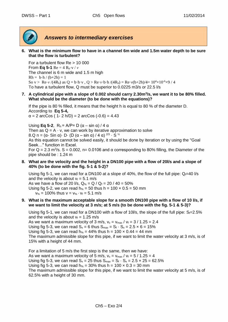
DWSS ndash Part 1 Ch5 Open flows 11022014
Ch5 ndash Exo 44
13 What is the flow going through a rectangular weir of 2m width with a crest height of 1 m and a height of water of 50cm We use eq 5-11 and 5-12
52hg2LcQ (1)
where L = 2 [m] h = 05 [m] z = 1 [m]
4340
105
05501
16051000
11041
zh
h501
16h1000
11041c
22
So sm679050819220434Q 325
DWSS ndash Part 1 Ch6 Pumps 11022014
Ch6 ndash Exo 114
Answers to basic exercises
1 For a pump of 50 m3h at 40 m head (NSasymp20) what is the expected hydraulic power pump efficiency mechanical power motor efficiency and power factor active and total electrical power
Hydraulic power Phydro=ρmiddotgmiddothmiddotQ
water density ρ=1 000 kgm3
gravitational constant g=981 ms2
manometric head h=40m
flow s00139m3600sh
h50mQ 3
3
So Phydro=1000times981times40times00139=5 450 W=545kW Pump efficiency ηp with figure 6-2 (efficiency of centrifugal pumps) for a NS of 20 and a flow of 50 m3h (yellow line) we get an efficiency of 73 Mechanical power Pmec=Phydroηpump=5 450073=7 466 W=747 kW Motor efficiency ηm with figure 6-1 (motor efficiency) For a rated power of approximately 75 kW and a 2-pole motor we get a motor efficiency of 093 Power factor with the same figure but the pink line we get a motor factor of 0895
Total power 897kW W89740730930895
00139409811000
ηηPF
QhgρS
pm
Active power Pelec=SmiddotPF=89737times0895=8032 W = 8 kW
2 What are the nominal head flow efficiency NPSH and power for the pumps a b and c
The nominal head and flow are the one corresponding to the highest efficiency Therefore
DWSS ndash Part 1 Ch6 Pumps 11022014
Ch6 ndash Exo 214
Pump a Pump b Pump c
Head h 63 m 14 m 65 m
Flow Q 100 m3h 375 m3h 2 200 m3s
Efficiency η 76 89 86
NPSH 6 m 3 m 7m
Power P 23 kW 155 kW 48 kW
3 What are the expected minimum and maximum flow for the pumps a b and c
The minimum flow corresponds to the functioning limit point (when the HQ diagram makes a kind of bump) For the maximum flow it is approximately when the lines on the charts end
Pump a Pump b Pump c
Minimum flow Qmin 20 m3h 200 m3h 1500 m3h
Maximum flow Qmax 140 m3h 500 m3h 2500 m3h
4 For the following system what will be the duty point with the pump a what is the power consumption
Elevation 200 masl
Temperature 20degc
All pipes are of new GI DN 175
Total punctual friction losses
- kp = 15 for the suction part
- kp= 5 for the delivery part
1) Estimate the flow
As the pump is already selected we can use its nominal flow for the first estimation (ie Q1 = 100 m3h)
2) Calculate hLP
hLP=punctual losses+linear losses= Lp
2
kk2g
v where
v=QA where s0027m3600sh
h100mQ 3
3
therefore for the first iteration
115ms
0175π4
1
0027
Dπ4
1
Qv
22
15m
215m
1 800 m 100 m 5m
DWSS ndash Part 1 Ch6 Pumps 11022014
Ch6 ndash Exo 314
kp=15+5=20
kL will depend on the velocity but we can either use the chart in the annexes (head losses for pipe under pressure) or use equations 4-15 and 4-19
D
Lλk L where lamda is calculated using eq 4-19
To use eq 419 we need the Reynolds number
102012101
0175115
ν
DvRe
6
which allows us to calculate λ=0020
L is the length of all the pipes L=5+15+100+215+1800=1928 m
D is the diameter 0175m
52181750
19280200kL with equation 4-15 and 4-19
1621m2185209812
115)k(k
2g
vh
2
Lp
2
LP
3) Calculate the total head
3921m1621m15)215(hhh lossesstatictot
4) Find a new Q (Q2)
Looking back in the HQ chart the flow corresponding to a head of 392m is 150 m3h To find this value it is necessary to extrapolate the right hand-side of the chart by extending the end of the curve This is shown in the following chart The purple line is the QP curve given and the blue line is the network curve which can be calculated as explained previously as a function of the flow
5) Iterate
For the next iteration we will take the average between the flow with which we started our calculations (Q1 100 m3h) and the flow we obtained at the end (Q2 150 m3h) which gives us a flow of 125 m3h
The iteration are shown in the following table At the end we find a flow of 130 m3h
90
40
50
60
70
80
20
30
Head h
(m
)
120 140 160 80 100 60 40 20 Q1 Q2 Qduty
DWSS ndash Part 1 Ch6 Pumps 11022014
Ch6 ndash Exo 414
it Q1 m3h Q m3s v Re lamda kL stat
head linear loss
punctual loss
total loss h tot
Q2 m3h
0 100 0028 115 202 101 0019 83 2185 23 1485 136 1621 3921 150
1 125 0035 144 252 626 0019 52 2151 23 2285 212 2497 4797 135
2 130 0036 150 262 732 0019 48 2146 23 2465 230 2695 4995 130
In order to find the corresponding power consumption we look in the QP chart and find a power consumption of 26kW
Answers to intermediary exercises
5 What is the number of poles and the slip value of the motor for the pumps a b and c
For this question we use Eq 6-5 and the corresponding table The number of rotation per minute (n) is written on the very top of each graph series for each pump We then look in the table to find the frequency and number of poles to which it corresponds The number n in the table might not correspond exactly to the number of the n indicated on the graph as the slip value varies from one motor to another After that we have only one unknown in eq 6-5 which becomes solvable
slip
nbPoles
f260n Therefore n-
nbPoles
f260slip
a) The number n=2 900 corresponds to 50 Hz and 2 poles
RPM10029002
50260slip
b) The number n=1 450 corresponds to 50 Hz and 4 poles
RPM5014504
50260slip
c) The number n=980 corresponds to 50 Hz and 6 poles
RPM209806
50260slip
6 What is the specific speed for the pumps a b and c
We use Eq 6-6 where Q and h are the nominal flows and heads found in 2
a)
2363
36001002900
h
QnN
750
50
075
05
s
This Ns correspond to a high head impeller described in the section about specific speed
DWSS ndash Part 1 Ch6 Pumps 11022014
Ch6 ndash Exo 514
The HQ chart has a curve rather flat
The efficiency curve is rounded The power consumption increases as the flow increases
b)
6514
36003751450
h
QnN
750
50
075
05
s
In this case we have a low head impeller
The HQ chart has a steeper curve with a functioning limit point Therefore the functioning range of this pump is smaller than the one used in a
The efficiency curve is less rounded than the one in a (more pointed at the top)
The power consumption is not linear but in overall decreases when the flow increases
c)
18856
36002200980
h
QnN
750
50
075
05
s
In this case we have an axial flow impeller
The HQ chart is even steeper curve with a functioning limit point The functioning range of this pump is very small for this kind of pumps
The efficiency curve is more pointed
The power consumption is not linear but in overall decreases when the flow increases The average slope of this line is steeper than the one in b
7 If we want to adjust the working point of the pump used in exercise 4 to the nominal point with a throttling system what should be the size of the orifice what would be the power consumption
The best efficiency (nominal point) of this pump is for a flow of 100 m3h and a head of 65m Given that for a flow of 100 m3h the head losses are 162 m (first iteration of exercise 4) and the static head stays at 23m the head losses that the orifice will have to create are
hp-orifice=63m-23m-162m=238m
DWSS ndash Part 1 Ch6 Pumps 11022014
Ch6 ndash Exo 614
With eq 4-14 we have
2g
vkh
2
oporifice-p where v is the velocity corresponding to a flow of 100m3h
1155
0175π4
1
1003600
Dπ4
1
Qv
22
ms (again this velocity can be read from the first
iteration exercise 4)
Therefore 0531155
9812238
v
2ghk
22
orifice-p
op
Therefore if we choose a sharp orifice we find (with the losses due to orifice chart in chapter 4) a dD ratio of 029 Given that our D=175mm d=029times175=51mm (which is the diameter of the orifice the edge of the orifice being sharp)
The power consumption will then be (looking in HP chart) of 23kW
This corresponds to a reduction of 13 compared to the system as it is working in exercise 4
8 With the same situation as exercise 4 what would be the new flow and power consumption if we decrease the rotation speed so that it reaches 80 of its initial value
The first thing is to define a new HQ curve For this we calculate the flow and the head at minimal maximal and optimal points
1
1
212 08Q
n
nQQ
1
2
1
212 064h
n
nhh
Therefore
90
40
50
60
70
80
20
30
Head h
(m
)
120 140 160 80 100 60 40 20
Static head
Head losses wo orifice
Head losses due to orifice
system curve with orrifice
system curve without orrifice
pump characteristic curve
DWSS ndash Part 1 Ch6 Pumps 11022014
Ch6 ndash Exo 714
100 80 100 80
Qmin 20 m3h 16 m3h hmax 80 m 52 m
Qopt 100 m3h 80 m3h hopt 63 m 40 m
Qmax 140 m3h 112 m3h hmin 45 m 29 m
The HQ curve will look like the one given but shifted to the bottom and right Knowing that we can draw the HQ curve of the pump It looks like that
Next we do the same as with point 4 with this new HQ curve
1) Estimate the flow
We take the nominal flow ie Q1=80 m3h
2) Calculate hLP
HLP=punctual losses+linear losses= Lp
2
kk2g
v where
092ms
0175π4
1
803600
Dπ4
1
Qv
22
kp=15+5=20
D
Lλk L where lamda is calculated using eq 4-19
681161101
0175092
ν
DvRe
6
which allows us to calculate λ=0020
L is (as for point 4) 1928 m and D is 0175m
52221750
19280200kL with equation 4-15 and 4-19
m55102225209812
092)k(k
2g
vh
2
Lp
2
LP
3) Calculate the total head
335mm51015)215(hhh lossesstatictot
50
60
70
30
40
Head h
(m
)
120 140 160 80 100 60 40 20
80
Qmin Qopt Qmax
hmin
hopt
hmax
DWSS ndash Part 1 Ch6 Pumps 11022014
Ch6 ndash Exo 814
4) Find a new Q (Q2)
Looking back at the pump characteristics the flow corresponding to a head of 335m is 105m3h This is shown in the following chart As before the purple line is the QP curve given and the blue line is the network characteristics which is the same as the one drawn in point 4
5) Iterate
The average between Q1 (80 m3h) and the flow we obtained at the end Q2 (105 m3h) which gives us a flow of 925 m3h
The iteration are shown in the following table At the end we find a flow of 95 m3h
it Q1 m3h Q m3s v Re lamda kL
stat head
linear loss
Punctual loss
total loss h tot
Q2 m3h
0 80 0022 092 1616812 0020 22250 23 968 087 1055 3355 105
1 925 0026 107 1869439 0020 21984 23 1279 116 1395 3695 97
2 9475 0026 109 1914912 0020 21942 23 1339 122 1461 3761 96
For the power consumption knowing that the flow is 95 m3h and that the power consumption
for this flow is 22 kW we will have 113kW0822n
nPP
3
3
1
212
As it can be noticed the power consumption passes from 26 kW without adjustment to 23kW with a throttling system and to 113 kW with a speed reduction system Compared with a throttling system (where we have almost the same flow reduction) the power consumption with a speed decrease system is much more efficient
9 If the system is working as per exercise 4 what is the maximum suction height And what is the maximum suction height if it is working as in exercise 7
The maximum suction head is when it is equal to the height of the water column minus the head losses in the suction part and the NPSH required by the pump
rS-LPva
suc NPSHhgρ
PPh
At 200 masl the atmospheric pressure is 98 000 Pa (chart chapter 2 page 3) In this exercise we want to avoid cavitation Therefore we have to take the minimum pressure on the chart (light blue line) representing the smallest water column The vapour pressure for water at 20degC is 2340 Pa (figure 2-3)
The height of the water column is mg
PP va 7599811000
234098000
The head losses in the suction part are calculated as follow
40
50
60
20
30
Head H
(m
)
120 140 160 80 100 60 40 20
Q1 Q2 Qduty
DWSS ndash Part 1 Ch6 Pumps 11022014
Ch6 ndash Exo 914
Lp
2
LP kk2g
vh where v=QA and kp=15 (punctual losses in the suction part)
The NPSHr is given in the chart NPSH versus flow
a) When the system is working as per exercise 4
The flow for this system is 130 m3h
The height of the water column is 975m
The head losses in the suction part we have
- kp for the suction part that is 15
- 11850175
10650019
D
LλkL where lambda is from the last iteration of point 6
L=5+15+100=1065 and D is the diameter 0175m
m0831185)(159812
51kk
2g
vh
2
Lp
2
LP
The NPSH For a flow of 130 m3h we find a NPSH of 8 m
Therefore the maximum is 133m8308759hsuc this negative number indicates
clearly that the system designed in point 6 only works if the pump is placed at least 135m below the water level If not cavitation will occur will damage the pump and reduce the flow
b) When the system is working as per exercise 7 (adjustment with a throttling system)
The height of the water column stays at 975m
The head losses in the suction part we have
- kp = 15 for the suction part
- 12070175
10650020
D
LλkL where lamda was recalculated for this flow with eq
419
189m)0712(159812
171kk
2g
vh
2
Lp
2
LP
The NPSH For a flow of 100 m3h we find a NPSH of 6 m
Therefore the maximum is 186m6189759h suc This value being higher than 15 m
(which is the suction height of the pump as it is designed in point 6) indicates that cavitation will not occur with this system
The maximum suction height between point a and b is increased because the flow is decreased which will decrease the head losses and the NPSH required by the pump Thus if we want this system to work without cavitation the flow has to be reduced by throttling trimming or speed reduction
DWSS ndash Part 1 Ch6 Pumps 11022014
Ch6 ndash Exo 1014
Answers to advanced exercises
10 For the system used in exercise 7 (with a throttling system) knowing that the intake water level varies of plus or minus 2 meters what would be the max and min flow what would be the max suction height
a) With plus 2 meters
The flow
We have to do the same iterations as it was done in exercise 4 This time the static head is 21m instead of 23m We can begin the iteration at 100 m3h since the flow will be practically the same (the static head does not change much)
The punctual losses coefficient is equal to the punctual losses in the suction part and delivery part plus the one of the orifice kp=15+5+350=370
it Q
m3h Q
m3s V
ms Re lamba kL
H static
Linear losses
Punctual losses
Total loss h tot
Q2 m3h
0 100 0028 115 2021015 0020 21851 21 1485 2515 4001 6101 1048
1 1024 0028 118 2069280 0020 21813 21 1554 2637 4191 6291 998
2 1011 0028 117 2043199 0020 21833 21 1517 2571 4088 6188 1025
3 1018 0028 118 2057735 0020 21822 21 1538 2607 4145 6245 1010
Thus by decreasing the static head the flow is increased of about 1 Q= 101 m3h
The maximum suction height (for this water level) is calculated as in exercise 9
o the height of the water column is 975 m
o the head losses in the suction part are
921)1750
51060200(15
9812
181
D
Lk
2g
vh
2
p
2
LP
m
o the NPSH is around 6m for a flow of 101 m3h
Therefore the maximum suction height is 975m-192m-6m=184
It must be noticed that it is 184m above the water level for which we calculated the flow which is 2 meters above the average suction level Therefore when the water level is 2m above the
hstat
Minus two meter b
Plus two meters a Average suction level
90
40
50
60
70
80
20
30
Head H
(m
)
120 140 160 80 100 60 40 20 Qa Qb
DWSS ndash Part 1 Ch6 Pumps 11022014
Ch6 ndash Exo 1114
average water level the pump should be placed at a maximum of 384m above the average water level
b) with minus 2 meters
The flow
We have to do the same iterations as it was done before This time the static head is 25m instead of 23m Again we start at a flow of 100 m3h
it Q m3h Q m3s v Re lamda kL
stat head linear loss
punctual loss total loss h tot Q2
0 1000 0028 115 2021015 0020 21851 25 1485 2515 4001 6501 941
1 970 0027 112 1960891 0020 21902 25 1402 2368 3769 6269 1004
2 987 0027 114 1994890 0020 21873 25 1449 2451 3899 6399 969
3 978 0027 113 1976407 0020 21888 25 1423 2405 3828 6328 988
4 983 0027 114 1986684 0020 21880 25 1437 2430 3868 6368 977
5 980 0027 113 1981039 0020 21884 25 1429 2417 3846 6346 983
(The number of iterations necessary to converge on the result has increased because the system curve is steeper which makes the iteration process less efficient)
This time by increasing the static head the flow is decreased of about 2 Q= 98 m3h
The maximum suction height (for this water level) is calculated as before
o the height of the water column is 975 m
o the head losses in the suction part are
m781)1750
51060200(15
9812
131
D
Lk
2g
vh
2
p
2
LP
o the NPSH is around 6m for a flow of 98 m3h
Therefore the maximum suction height is 975m-178m-6m=197m
This height corresponds to a height of 197m above the water level for which we calculated the flow (which is 2 meters below the average suction level) Therefore the pump should be placed just below the average water level or lower (2m-197m=003m=3cm) This level is (not surprisingly) lower than the one obtained in a Therefore this is the value to be considered when doing the design to find the elevation of the pump avoiding cavitation As a result if the pump is place 15 m above the surface level (as it is the case in exercise 7) it will cavitate when the water level will drop down As it can be seen the variation of the water level in the intake tank has a big impact on cavitation and should be taken into account when doing calculations
11 With a frequency inverter what should be the percent speed reduction to adjust the system to the nominal point of the pump What is the corresponding flow
As it is explained in the section about speed reduction the line of nominal points with a speed reduction is parable In order to find the point where the system is at its nominal point we will have to find the place where the nominal point line crosses the system curve This is shown on the following graph
DWSS ndash Part 1 Ch6 Pumps 11022014
Ch6 ndash Exo 1214
0
20
40
60
80
100
120
140
0 50 100 150
Flow (m3h)
Head
(m
)
System curve
Line of nominal point
Pump curve w ithout speed
reduction
Pump curve w ith x speed
reduction
First we have to find the equation of this parable A parable is from the type
y=ax2+bx+c In our case it is hn=aQn2+bQn+c (hn and Qn indicates the nominal head and
nominal flow respectively)
We know that it passes by the origin thus c=0 Therefore the equation of the parable will be from the type
hn=aQn2+bQn
To find the coefficient a and b we need two points on this curve
If we do not change the system the nominal point is Qn=100 m3h and hn=63 which will be the first of the two needed points
The second point (which is whichever point on the curve with r rotation speed) will have apostrophe (Hn and Qn) to make the difference between the first (with 100 speed) and second point (r speed)
2
n
n
n
n
n
2
n
n
n
2
nn
rhh(4)
rQQ(3)
QbQah(2)
QbQah(1)
Substituting (3) and (4) into (2) we get
rbQraQrh)5( n
22
n
2
n
which simplifies to (dividing by r)
n
2
nn bQraQrh(6)
From (1) we know that
2
nnn QahQb)7(
Putting (7) back into (6) we get
2
nn
2
nn QahrQarh)8(
DWSS ndash Part 1 Ch6 Pumps 11022014
Ch6 ndash Exo 1314
which can be written as
1)(rQa1)(rh)9( 2
nn
If follows that
2
n
n
Q
ha)10( In that case given that Qn=100 m3h and hn=63 we have 30006
100
63a
2
To find the coefficient b we use (10) and (1) and find
n
2
n2
n
nn QbQ
Q
hh)11(
which gives us b=0
Therefore our equation of the line of nominal point is 200063Qh
To find the intersection of the line of nominal point and the system curve we will have to iterate in a slightly different way as before
For a given flow Q1 we will estimate the losses and the total head (static head plus head losses) as it was done before
Then for this head we will find the corresponding flow Q2 on the line of nominal points To find the nominal flow for a given head we solve the following equation for Q
0h00063Q2 which gives us 00063
hQ
This time Q2 can directly be taken for the next iteration (no need to do the average between Q1 and Q2) This is because between Q1 and Q2 we do not cross the intersection as it was the case for the previous iterations (this can be seen in the following figure) Therefore we get closer to the results every time and Q2 can be taken for the next iteration
We will start the iteration at the nominal flow without speed reduction system namely 100 m3h The iterations are shown in the following table
0
20
40
60
80
100
120
140
0 50 100 150
System curve Line of nominal point
Q1 Q2
DWSS ndash Part 1 Ch6 Pumps 11022014
Ch6 ndash Exo 1414
it Q m3h
Q m3s v Re lamda kL
stat head
linear loss
punctual loss
total loss total h Q2
0 100 0028 115 202102 002 21851 23 148538 13595 162134 3921 789
1 7889 0022 091 159447 002 22277 23 942562 08462 102718 3327 727
2 7267 002 084 146872 002 22441 23 805645 0718 877446 3177 71
3 7102 002 082 143529 002 22489 23 771023 06857 839593 314 706
4 7059 002 082 142671 002 22501 23 762262 06775 830015 313 705
At the end we get approximately a flow of 70 m3h
Given that 1
2
1
2
n
n
Q
Q and that we have 07
100
70
Q
Q
1
2 it follows that 07n
n
1
2
Therefore the speed reduction should be of 70
For the pump a we have a frequency of 50 Hz Given that the rotation speed is directly proportional to the frequency the frequency will have to be reduced to 70 of its initial value which is 35 Hz
DWSS ndash Part 1 Ch7 Water hammer 11022014
Ch7 ndash Exo 17
Answers to basic exercises
1 Draw the pressure and the velocity versus the time (Lc) at the middle of the pipe for an instantaneous valve closure neglecting head losses
The surge will arrive at the middle of the pipe after half of the time needed to travel the pipe L2c and come back after two times this time 2L2c=Lc
2 What are the velocity of the pressure wave (c) the head surge (Δh) and the return time in a cast iron pipe DN200 of 3 kilometres for a instantaneous decrease of velocity of 15 ms
With the table of Cast iron pipe in the annexe N we find with DN200 the value of c=1216 ms To find Δh we have to multiple the given value by the actual velocity Δh=124times15=186 m To find the return time we have to multiple the given value by the actual length in km Tr=16times3=48 s
In this case the pressure surge is huge (almost 18 bar) but the return time very short thus if it is possible to extend the closure or stopping time to 10 s the surge would be divided by 2 (9 bar) and with 20 s by 4 (ie 45 bar)
3 What are the velocity of the pressure wave (c) the head surge (Δh) and the return time in a PE pipe SDR11 of 5 kilometres for a instantaneous decrease of velocity of 2 ms
With the table of PE pipe in the annexe N we find with SDR11 (the diameter of the pipe is not needed the water hammer will be the same for the all series) the value of c=342 ms To find Δh we have to multiple the given value by the actual velocity Δh=35times2=70 m To find the return time we have to multiple the given value by the actual length in km Tr=58times5=29 s
In this case we can see that the pressure surge is smaller (~7 bar) but that the return time is quite important almost half minute before the surge is back
4 What are the velocity of the pressure wave (c) the head surge (Δh) and the return time in a PVC pipe SDR17 OD 200 of 2 kilometres for a instantaneous closure with an initial velocity of 1 ms
With the table of PVC pipe ODgt100 in the annexe N we find with SDR17 (the water hammer will be the same for the all series with ODgt100) the value of c=490 ms The Δh is the one in the table as the velocity is of 1 ms Δh=50 m To find the return time we have to multiple the given value by the actual length in km Tr=41times2=82 s
In this case we can see that the pressure surge is quite small (~5 bar) and the return time not too long (less than 10 s) Thus this pipe should be not too much at risk
pre
ssure
time
L2c
-ΔP
P0
t0 Lc 2Lc 3Lc 4Lc
+Δ
P
1 2
5Lc
3 4 Phases
t0
Reversed flow
Ve
locity
v0
Lc Lc
time Lc 2Lc 3Lc 4Lc 5Lc
DWSS ndash Part 1 Ch7 Water hammer 11022014
Ch7 ndash Exo 27
5 What length of the previous pipe will have a reduced surge if the closure time is of 41 second
The length with reduce surge is according to eq 74 is Lred = Tc c 2 = 41 times 490 2 = 1000 m Thus with a decreasing time of half the return time half of the pipeline will have reduced pressure durge
6 Neglecting losses draw the envelope scheme for the previous pipe knowing that its profile is as per the attached table Is the pipe safe (assuming a linear front wave) If not what can be done
Pump Pt 1 Pt 2 Pt 3 Tank
Pipe length 0 500 1000 1500 2000
Elevation 0 10 30 30 70
We can see that a part of the pipeline (between 750 and 1 200) will be exposed to depressure and that around 1 000 m it might even face cavitation There is no risk of pipe burst (over pressure) as the maximum pressure (hstat + Δh = 120) is smaller than the pipe PN (~125 m) In order to avoid this depressure in the pipe the following could be done - Increase the stopping time - Install air valves letting air come into the pipe in the zone at risk
7 For the previous system what should be the closure time to limit the Δh at 30m
According to Eq 75 s61330819
120002
hg
v2LT
Tg
v2Lh
max
inc
c
inmax
Thus to reduce the Δh to 30 m the closure time should be of 136 s In theory this would be also valid for a cast iron pipe or any material with a return time for this system smaller than 136 s
Δh=50m
Static line
Lred = 1 000 m
Zone at risk
Min acceptable pressure
Max acceptable pressure
Δh=50m
500 1 000 1 500 2 000
70
30
10
120 125
Pipe length [m]
Elevation [m]
-8
DWSS ndash Part 1 Ch7 Water hammer 11022014
Ch7 ndash Exo 37
Answers to intermediary exercises
8 Draw the pressure and the velocity versus the time (Lc) at the middle of the pipe for an instantaneous valve closure taking into consideration head losses
The surge will arrive at the middle of the pipe after half of the time needed to travel the pipe L2c and come back after two times this time 2L2c=Lc
9 What are the velocity (c) the head surge (Δh) and the return time (Tr) of the pressure wave in a cast iron pipe DN200 (e=64 mm Kpipe=140 GPa) of 3 km if a pump of 170 m3h instantaneously stops working with a temperature of water of 45deg
We calculate c with Eq 7-1
pipe
water
water
K
K
e
D1
ρKc
where at 45deg Kwater is 229 GPa and ρ=9902 kgm3
The thickness e is 64 mm KCI is 140 GPa
The diameter D can be estimated as the nominal diameter (DN) so 200 mm
so ms 1237
10140
10229
64
2001
990210229
K
K
e
D1
ρKc
9
9
9
pipe
water
water
Given that the flow is totally stopped
ms 150
102004
π
1703600
A
QvΔv
23
The head surge is found with equation 7-1 Δh = Δvmiddotcg=15 times 1237 981 = 1896 m
The return time is found with equation 7-3 Tr= 2Lc= 2 times 3000 1237 = 485 s
If we compare these results with the exercise 2 we can see that they are very close the difference of taking in to consideration the water temperature of 45deg make a difference of 15 on the head surge and of 1 on the return time
pre
ssure
time
L2c
-ΔP
P0
t0 Lc 2Lc 3Lc 4Lc
+Δ
P
1 2
5Lc
3 4 Phases
t0
Reversed flow
Ve
locity
v0
Lc Lc
time Lc 2Lc 3Lc 4Lc 5Lc
DWSS ndash Part 1 Ch7 Water hammer 11022014
Ch7 ndash Exo 47
10 For the previous pipe we want to limit the head surge at 100m by having a longer stopping time what should be in this case TC
According to equation 7-5 we have s 179100819
5130002
hg
v2LT
max
inc
BY increasing significantly the closure time we will have almost half of the flow when the head surge is coming back therefore the Δv is divided by two dividing thus also the head surge by two
11 What are the velocity (c) the head surge (Δh) and the return time (Tr) of the pressure wave in a PE80 pipe PN125 OD200 (KPE=07 GPa e=182mm) of 5 km if a pump of 150 m3h instantaneously stops working with a temperature of water of 20deg
We calculate c with Eq 7-1
pipe
water
water
K
K
e
D1
ρKc
where at 20deg Kwater is 22 GPa and ρ=9982 kgm3
The nominal thickness for this pipe is given 182 mm (an average of 192 could be used)
The bulk modulus KPE is given as 07 GPa
The internal diameter D is thus per Annexe B 1636 mm
so ms 742
1070
1022
182
16361
99821022
K
K
e
D1
ρKc
9
9
9
pipe
water
water
Given that the flow is totally stopped
ms 1982
102004
π
1503600
A
QvΔv
23
The head surge is found with equation 7-1 Δh = Δvmiddotcg=1982 times 274 981 = 555 m
The return time is found with equation 7-3 Tr= 2Lc= 2 times 5000 274 = 364 s
This time if we compare these results with the exercise 3 we can see that they are not so close as the bulk modulus given is quite different from the one used in the table in annexe N
12 What are the friction coefficient (KLP) and the head losses (hLP) of the previous pipe with a roughness of 007 mm neglecting the punctual losses What is the attenuation of the negative head surge due to the losses at the tank
With equation 4-9 we find Re = D middot v ν = 1636 times 1982 101 times 10-6 = 322 000
With equation 4-19 or fig 4-5 we find λ = 00147
As the singular losses are neglected we find with equations 4-15
KLP = λ middot L D = 00147 times 5 000 01636 = 449
hLP = v2 middot λ 2g = 19822 times 449 (2 times 981) = 899 m
Thus the attenuation of the negative head surge at the tank is equal to hlosses2 about 45m In this situation where the losses are quite high as the velocity is important we can see that the remaining negative head surge at the tank is only of 10m thus the importance to take them in to account
DWSS ndash Part 1 Ch7 Water hammer 11022014
Ch7 ndash Exo 57
13 What are the attenuation of head surge at the valve (hv-att) the remaining velocity at the tank (vt1) and the attenuation of the positive head surge at the tank (ht-att) of the previous pipe
With equation 7-6 we find m 8254499812
7421-274
982144921
2gk
c1-c
vk21
h
2
2
LP
2
2
inLP
att-v
With equation 4-9 we find
m 52494981
7421-274
6071982149412
gk
c1-c
vvk12
h
ms 60712744
9821449
4c
vkv
2
2
LP
2
2
t1inLP
att-t
22
inLPt1
Thus when the surge arrive to the tank the velocity in the depression zone reaches 1607 ms This explains why the negative head surge is so small at the tanks as the difference of velocity is then only of 1982-1602=0375 ms
The attenuation of the positive head surge at the valve is of 258 m thus the positive head surge at the valve is of 555 - 258 asymp 30 m NB this value as to be added at the static level not at the dynamic one This value is much smaller than the initial head losses (899 m) thus the positive head surge is not affecting the pipe at the valve
The attenuation of the positive head surge at the tank is of 25 m thus the positive head surge at the tank is of 555 ndash 899 2 ndash 25 asymp 8 m This remaining positive head surge at the tank is very small
See the next exercise correction for an illustration of these results
14 For the previous pipe draw the developed profile of the pipeline the static and dynamic lines and the envelope schemes knowing that its profile is as per the attached table Is the pipe safe If not what can be done
Pump Pt 1 Pt 2 Pt 3 Tank
Pipe length 0 1000 1000 1000 2000
Elevation 0 0 5 10 30
As explain in the section 76 the developed profile should be used but as the slopes are small it doesnt make a big difference if it is taken into consideration or not
All the values calculated in the previous exercises were reported in this chart
It can be seen that the superior envelope is much lower than the maximum acceptable pressure thus there is no risk of pipe burst in case of water hammer
However the inferior level is lower than the ground level even lower than the cavitation line (minimum acceptable pressure) thus depressure and cavitation will happen in this pipeline if it is not protected
Possible solutions might include a pump bypass system or air valve Nevertheless into this situation the best would be to increase the diameter of the pipe decreasing also the losses and necessary PN for the pipe this will thus decrease the thickness and further the head surge
DWSS ndash Part 1 Ch7 Water hammer 11022014
Ch7 ndash Exo 67
15 What would be the effect on the head surge on the previous exercises of having a Youngs modulus (KPE)of 11 GPa instead of 07 GPa
The surge velocity will be at 341 ms instead of 274 ms increasing the head surge at 70 m instead of 56 m This will significantly increase the problematic of the depressure at the valve even for bigger diameters This shows the importance to have a good information from the supplier about the properties of the pipes and in case of doubt to take a good margin between the envelope and the maximum or minimum tolerable pressure
16 For exercise 2-4 what would be the change in ID (DN for metallic pipe) following the change in pressure due to water hammer
In order to calculate ΔD we use a formula from chapter 1 (Eq 1-5)
2e
D
K
ΔPDΔD
K is the Youngs modulus of the pipe material For the first exercise to find ΔD in mm we have
0026mm642
200
10125
1053400200ΔD
9
Therefore when the pipe will be in overpressure the DN will be Do=200+0026=200026 mm (the pipe will be expanded)
When the pipe will be in under pressure the DN will be Du= 200-0026=19997
Answers to advanced exercises
11m
Developed profile of the pipeline
-30
-10
10
30
50
70
90
110
130
0 500 1000 1500 2000 2500 3000 3500 4000 4500 5000
Dynamic or piezo line
Static line
Overpressure envelope
Depressure envelope
Pipeline
Min acceptable pressure
Max acceptable pressure
0
Elevation
PN
of
the p
ie ~
123m
Head losses
~90m
Attenuated positive head surge at the
valve ~30m
Tank elevation
~30m
Depressure ~56m
Pipe length [m]
Cavitation ~9m Head losses2
~45m
Attenuation of head surge at the valve
~26m Head losses2 +
ht-att ~48m
8m
DWSS ndash Part 1 Ch7 Water hammer 11022014
Ch7 ndash Exo 77
The same procedure is done for exercise 3 amp 4 The results are shown it the following table
Ex ΔP Pa DN or ID mm e mm K GPa ΔD mm Do mm Du mm
2
3
4
We can draw the following conclusion
even if the ΔP is bigger for cast iron the change in diameter will be less than for PE (because PE is easily distorted)
even if the ΔP is bigger for exercise 4 than for 3 the change in pipes diameter will be bigger for 3 because the wall thickness is smaller (which makes the pipe more easily distorted)
It can be noticed that the expansion due to changes in pressure in the pipe is not significant because even for PE pipe with a bigger expansion it is around half a millimetre added to the outside diameter which is less than the tolerance margin for PE pipe For example for a PE pipe having an OD of 200 mm the maximum outside diameter will be of 2012 mm (which is bigger than 2005 obtained with pressure expansion) These calculations were done for expansion due to pressure changes only because of water hammer (thus ignoring the initial pressure in the pipe) This means that the diameter can be more expanded because the total change in pressure will be bigger Furthermore if we have an initial pressure it must be checked that the PN of the pipe can bear the total pressure (initial pressure +ΔP)

DWSS ndash Part 1 Ch6 Pumps 11022014
Ch6 ndash Exo 614
With eq 4-14 we have
2g
vkh
2
oporifice-p where v is the velocity corresponding to a flow of 100m3h
1155
0175π4
1
1003600
Dπ4
1
Qv
22
ms (again this velocity can be read from the first
iteration exercise 4)
Therefore 0531155
9812238
v
2ghk
22
orifice-p
op
Therefore if we choose a sharp orifice we find (with the losses due to orifice chart in chapter 4) a dD ratio of 029 Given that our D=175mm d=029times175=51mm (which is the diameter of the orifice the edge of the orifice being sharp)
The power consumption will then be (looking in HP chart) of 23kW
This corresponds to a reduction of 13 compared to the system as it is working in exercise 4
8 With the same situation as exercise 4 what would be the new flow and power consumption if we decrease the rotation speed so that it reaches 80 of its initial value
The first thing is to define a new HQ curve For this we calculate the flow and the head at minimal maximal and optimal points
1
1
212 08Q
n
nQQ
1
2
1
212 064h
n
nhh
Therefore
90
40
50
60
70
80
20
30
Head h
(m
)
120 140 160 80 100 60 40 20
Static head
Head losses wo orifice
Head losses due to orifice
system curve with orrifice
system curve without orrifice
pump characteristic curve
DWSS ndash Part 1 Ch6 Pumps 11022014
Ch6 ndash Exo 714
100 80 100 80
Qmin 20 m3h 16 m3h hmax 80 m 52 m
Qopt 100 m3h 80 m3h hopt 63 m 40 m
Qmax 140 m3h 112 m3h hmin 45 m 29 m
The HQ curve will look like the one given but shifted to the bottom and right Knowing that we can draw the HQ curve of the pump It looks like that
Next we do the same as with point 4 with this new HQ curve
1) Estimate the flow
We take the nominal flow ie Q1=80 m3h
2) Calculate hLP
HLP=punctual losses+linear losses= Lp
2
kk2g
v where
092ms
0175π4
1
803600
Dπ4
1
Qv
22
kp=15+5=20
D
Lλk L where lamda is calculated using eq 4-19
681161101
0175092
ν
DvRe
6
which allows us to calculate λ=0020
L is (as for point 4) 1928 m and D is 0175m
52221750
19280200kL with equation 4-15 and 4-19
m55102225209812
092)k(k
2g
vh
2
Lp
2
LP
3) Calculate the total head
335mm51015)215(hhh lossesstatictot
50
60
70
30
40
Head h
(m
)
120 140 160 80 100 60 40 20
80
Qmin Qopt Qmax
hmin
hopt
hmax
DWSS ndash Part 1 Ch6 Pumps 11022014
Ch6 ndash Exo 814
4) Find a new Q (Q2)
Looking back at the pump characteristics the flow corresponding to a head of 335m is 105m3h This is shown in the following chart As before the purple line is the QP curve given and the blue line is the network characteristics which is the same as the one drawn in point 4
5) Iterate
The average between Q1 (80 m3h) and the flow we obtained at the end Q2 (105 m3h) which gives us a flow of 925 m3h
The iteration are shown in the following table At the end we find a flow of 95 m3h
it Q1 m3h Q m3s v Re lamda kL
stat head
linear loss
Punctual loss
total loss h tot
Q2 m3h
0 80 0022 092 1616812 0020 22250 23 968 087 1055 3355 105
1 925 0026 107 1869439 0020 21984 23 1279 116 1395 3695 97
2 9475 0026 109 1914912 0020 21942 23 1339 122 1461 3761 96
For the power consumption knowing that the flow is 95 m3h and that the power consumption
for this flow is 22 kW we will have 113kW0822n
nPP
3
3
1
212
As it can be noticed the power consumption passes from 26 kW without adjustment to 23kW with a throttling system and to 113 kW with a speed reduction system Compared with a throttling system (where we have almost the same flow reduction) the power consumption with a speed decrease system is much more efficient
9 If the system is working as per exercise 4 what is the maximum suction height And what is the maximum suction height if it is working as in exercise 7
The maximum suction head is when it is equal to the height of the water column minus the head losses in the suction part and the NPSH required by the pump
rS-LPva
suc NPSHhgρ
PPh
At 200 masl the atmospheric pressure is 98 000 Pa (chart chapter 2 page 3) In this exercise we want to avoid cavitation Therefore we have to take the minimum pressure on the chart (light blue line) representing the smallest water column The vapour pressure for water at 20degC is 2340 Pa (figure 2-3)
The height of the water column is mg
PP va 7599811000
234098000
The head losses in the suction part are calculated as follow
40
50
60
20
30
Head H
(m
)
120 140 160 80 100 60 40 20
Q1 Q2 Qduty
DWSS ndash Part 1 Ch6 Pumps 11022014
Ch6 ndash Exo 914
Lp
2
LP kk2g
vh where v=QA and kp=15 (punctual losses in the suction part)
The NPSHr is given in the chart NPSH versus flow
a) When the system is working as per exercise 4
The flow for this system is 130 m3h
The height of the water column is 975m
The head losses in the suction part we have
- kp for the suction part that is 15
- 11850175
10650019
D
LλkL where lambda is from the last iteration of point 6
L=5+15+100=1065 and D is the diameter 0175m
m0831185)(159812
51kk
2g
vh
2
Lp
2
LP
The NPSH For a flow of 130 m3h we find a NPSH of 8 m
Therefore the maximum is 133m8308759hsuc this negative number indicates
clearly that the system designed in point 6 only works if the pump is placed at least 135m below the water level If not cavitation will occur will damage the pump and reduce the flow
b) When the system is working as per exercise 7 (adjustment with a throttling system)
The height of the water column stays at 975m
The head losses in the suction part we have
- kp = 15 for the suction part
- 12070175
10650020
D
LλkL where lamda was recalculated for this flow with eq
419
189m)0712(159812
171kk
2g
vh
2
Lp
2
LP
The NPSH For a flow of 100 m3h we find a NPSH of 6 m
Therefore the maximum is 186m6189759h suc This value being higher than 15 m
(which is the suction height of the pump as it is designed in point 6) indicates that cavitation will not occur with this system
The maximum suction height between point a and b is increased because the flow is decreased which will decrease the head losses and the NPSH required by the pump Thus if we want this system to work without cavitation the flow has to be reduced by throttling trimming or speed reduction
DWSS ndash Part 1 Ch6 Pumps 11022014
Ch6 ndash Exo 1014
Answers to advanced exercises
10 For the system used in exercise 7 (with a throttling system) knowing that the intake water level varies of plus or minus 2 meters what would be the max and min flow what would be the max suction height
a) With plus 2 meters
The flow
We have to do the same iterations as it was done in exercise 4 This time the static head is 21m instead of 23m We can begin the iteration at 100 m3h since the flow will be practically the same (the static head does not change much)
The punctual losses coefficient is equal to the punctual losses in the suction part and delivery part plus the one of the orifice kp=15+5+350=370
it Q
m3h Q
m3s V
ms Re lamba kL
H static
Linear losses
Punctual losses
Total loss h tot
Q2 m3h
0 100 0028 115 2021015 0020 21851 21 1485 2515 4001 6101 1048
1 1024 0028 118 2069280 0020 21813 21 1554 2637 4191 6291 998
2 1011 0028 117 2043199 0020 21833 21 1517 2571 4088 6188 1025
3 1018 0028 118 2057735 0020 21822 21 1538 2607 4145 6245 1010
Thus by decreasing the static head the flow is increased of about 1 Q= 101 m3h
The maximum suction height (for this water level) is calculated as in exercise 9
o the height of the water column is 975 m
o the head losses in the suction part are
921)1750
51060200(15
9812
181
D
Lk
2g
vh
2
p
2
LP
m
o the NPSH is around 6m for a flow of 101 m3h
Therefore the maximum suction height is 975m-192m-6m=184
It must be noticed that it is 184m above the water level for which we calculated the flow which is 2 meters above the average suction level Therefore when the water level is 2m above the
hstat
Minus two meter b
Plus two meters a Average suction level
90
40
50
60
70
80
20
30
Head H
(m
)
120 140 160 80 100 60 40 20 Qa Qb
DWSS ndash Part 1 Ch6 Pumps 11022014
Ch6 ndash Exo 1114
average water level the pump should be placed at a maximum of 384m above the average water level
b) with minus 2 meters
The flow
We have to do the same iterations as it was done before This time the static head is 25m instead of 23m Again we start at a flow of 100 m3h
it Q m3h Q m3s v Re lamda kL
stat head linear loss
punctual loss total loss h tot Q2
0 1000 0028 115 2021015 0020 21851 25 1485 2515 4001 6501 941
1 970 0027 112 1960891 0020 21902 25 1402 2368 3769 6269 1004
2 987 0027 114 1994890 0020 21873 25 1449 2451 3899 6399 969
3 978 0027 113 1976407 0020 21888 25 1423 2405 3828 6328 988
4 983 0027 114 1986684 0020 21880 25 1437 2430 3868 6368 977
5 980 0027 113 1981039 0020 21884 25 1429 2417 3846 6346 983
(The number of iterations necessary to converge on the result has increased because the system curve is steeper which makes the iteration process less efficient)
This time by increasing the static head the flow is decreased of about 2 Q= 98 m3h
The maximum suction height (for this water level) is calculated as before
o the height of the water column is 975 m
o the head losses in the suction part are
m781)1750
51060200(15
9812
131
D
Lk
2g
vh
2
p
2
LP
o the NPSH is around 6m for a flow of 98 m3h
Therefore the maximum suction height is 975m-178m-6m=197m
This height corresponds to a height of 197m above the water level for which we calculated the flow (which is 2 meters below the average suction level) Therefore the pump should be placed just below the average water level or lower (2m-197m=003m=3cm) This level is (not surprisingly) lower than the one obtained in a Therefore this is the value to be considered when doing the design to find the elevation of the pump avoiding cavitation As a result if the pump is place 15 m above the surface level (as it is the case in exercise 7) it will cavitate when the water level will drop down As it can be seen the variation of the water level in the intake tank has a big impact on cavitation and should be taken into account when doing calculations
11 With a frequency inverter what should be the percent speed reduction to adjust the system to the nominal point of the pump What is the corresponding flow
As it is explained in the section about speed reduction the line of nominal points with a speed reduction is parable In order to find the point where the system is at its nominal point we will have to find the place where the nominal point line crosses the system curve This is shown on the following graph
DWSS ndash Part 1 Ch6 Pumps 11022014
Ch6 ndash Exo 1214
0
20
40
60
80
100
120
140
0 50 100 150
Flow (m3h)
Head
(m
)
System curve
Line of nominal point
Pump curve w ithout speed
reduction
Pump curve w ith x speed
reduction
First we have to find the equation of this parable A parable is from the type
y=ax2+bx+c In our case it is hn=aQn2+bQn+c (hn and Qn indicates the nominal head and
nominal flow respectively)
We know that it passes by the origin thus c=0 Therefore the equation of the parable will be from the type
hn=aQn2+bQn
To find the coefficient a and b we need two points on this curve
If we do not change the system the nominal point is Qn=100 m3h and hn=63 which will be the first of the two needed points
The second point (which is whichever point on the curve with r rotation speed) will have apostrophe (Hn and Qn) to make the difference between the first (with 100 speed) and second point (r speed)
2
n
n
n
n
n
2
n
n
n
2
nn
rhh(4)
rQQ(3)
QbQah(2)
QbQah(1)
Substituting (3) and (4) into (2) we get
rbQraQrh)5( n
22
n
2
n
which simplifies to (dividing by r)
n
2
nn bQraQrh(6)
From (1) we know that
2
nnn QahQb)7(
Putting (7) back into (6) we get
2
nn
2
nn QahrQarh)8(
DWSS ndash Part 1 Ch6 Pumps 11022014
Ch6 ndash Exo 1314
which can be written as
1)(rQa1)(rh)9( 2
nn
If follows that
2
n
n
Q
ha)10( In that case given that Qn=100 m3h and hn=63 we have 30006
100
63a
2
To find the coefficient b we use (10) and (1) and find
n
2
n2
n
nn QbQ
Q
hh)11(
which gives us b=0
Therefore our equation of the line of nominal point is 200063Qh
To find the intersection of the line of nominal point and the system curve we will have to iterate in a slightly different way as before
For a given flow Q1 we will estimate the losses and the total head (static head plus head losses) as it was done before
Then for this head we will find the corresponding flow Q2 on the line of nominal points To find the nominal flow for a given head we solve the following equation for Q
0h00063Q2 which gives us 00063
hQ
This time Q2 can directly be taken for the next iteration (no need to do the average between Q1 and Q2) This is because between Q1 and Q2 we do not cross the intersection as it was the case for the previous iterations (this can be seen in the following figure) Therefore we get closer to the results every time and Q2 can be taken for the next iteration
We will start the iteration at the nominal flow without speed reduction system namely 100 m3h The iterations are shown in the following table
0
20
40
60
80
100
120
140
0 50 100 150
System curve Line of nominal point
Q1 Q2
DWSS ndash Part 1 Ch6 Pumps 11022014
Ch6 ndash Exo 1414
it Q m3h
Q m3s v Re lamda kL
stat head
linear loss
punctual loss
total loss total h Q2
0 100 0028 115 202102 002 21851 23 148538 13595 162134 3921 789
1 7889 0022 091 159447 002 22277 23 942562 08462 102718 3327 727
2 7267 002 084 146872 002 22441 23 805645 0718 877446 3177 71
3 7102 002 082 143529 002 22489 23 771023 06857 839593 314 706
4 7059 002 082 142671 002 22501 23 762262 06775 830015 313 705
At the end we get approximately a flow of 70 m3h
Given that 1
2
1
2
n
n
Q
Q and that we have 07
100
70
Q
Q
1
2 it follows that 07n
n
1
2
Therefore the speed reduction should be of 70
For the pump a we have a frequency of 50 Hz Given that the rotation speed is directly proportional to the frequency the frequency will have to be reduced to 70 of its initial value which is 35 Hz
DWSS ndash Part 1 Ch7 Water hammer 11022014
Ch7 ndash Exo 17
Answers to basic exercises
1 Draw the pressure and the velocity versus the time (Lc) at the middle of the pipe for an instantaneous valve closure neglecting head losses
The surge will arrive at the middle of the pipe after half of the time needed to travel the pipe L2c and come back after two times this time 2L2c=Lc
2 What are the velocity of the pressure wave (c) the head surge (Δh) and the return time in a cast iron pipe DN200 of 3 kilometres for a instantaneous decrease of velocity of 15 ms
With the table of Cast iron pipe in the annexe N we find with DN200 the value of c=1216 ms To find Δh we have to multiple the given value by the actual velocity Δh=124times15=186 m To find the return time we have to multiple the given value by the actual length in km Tr=16times3=48 s
In this case the pressure surge is huge (almost 18 bar) but the return time very short thus if it is possible to extend the closure or stopping time to 10 s the surge would be divided by 2 (9 bar) and with 20 s by 4 (ie 45 bar)
3 What are the velocity of the pressure wave (c) the head surge (Δh) and the return time in a PE pipe SDR11 of 5 kilometres for a instantaneous decrease of velocity of 2 ms
With the table of PE pipe in the annexe N we find with SDR11 (the diameter of the pipe is not needed the water hammer will be the same for the all series) the value of c=342 ms To find Δh we have to multiple the given value by the actual velocity Δh=35times2=70 m To find the return time we have to multiple the given value by the actual length in km Tr=58times5=29 s
In this case we can see that the pressure surge is smaller (~7 bar) but that the return time is quite important almost half minute before the surge is back
4 What are the velocity of the pressure wave (c) the head surge (Δh) and the return time in a PVC pipe SDR17 OD 200 of 2 kilometres for a instantaneous closure with an initial velocity of 1 ms
With the table of PVC pipe ODgt100 in the annexe N we find with SDR17 (the water hammer will be the same for the all series with ODgt100) the value of c=490 ms The Δh is the one in the table as the velocity is of 1 ms Δh=50 m To find the return time we have to multiple the given value by the actual length in km Tr=41times2=82 s
In this case we can see that the pressure surge is quite small (~5 bar) and the return time not too long (less than 10 s) Thus this pipe should be not too much at risk
pre
ssure
time
L2c
-ΔP
P0
t0 Lc 2Lc 3Lc 4Lc
+Δ
P
1 2
5Lc
3 4 Phases
t0
Reversed flow
Ve
locity
v0
Lc Lc
time Lc 2Lc 3Lc 4Lc 5Lc
DWSS ndash Part 1 Ch7 Water hammer 11022014
Ch7 ndash Exo 27
5 What length of the previous pipe will have a reduced surge if the closure time is of 41 second
The length with reduce surge is according to eq 74 is Lred = Tc c 2 = 41 times 490 2 = 1000 m Thus with a decreasing time of half the return time half of the pipeline will have reduced pressure durge
6 Neglecting losses draw the envelope scheme for the previous pipe knowing that its profile is as per the attached table Is the pipe safe (assuming a linear front wave) If not what can be done
Pump Pt 1 Pt 2 Pt 3 Tank
Pipe length 0 500 1000 1500 2000
Elevation 0 10 30 30 70
We can see that a part of the pipeline (between 750 and 1 200) will be exposed to depressure and that around 1 000 m it might even face cavitation There is no risk of pipe burst (over pressure) as the maximum pressure (hstat + Δh = 120) is smaller than the pipe PN (~125 m) In order to avoid this depressure in the pipe the following could be done - Increase the stopping time - Install air valves letting air come into the pipe in the zone at risk
7 For the previous system what should be the closure time to limit the Δh at 30m
According to Eq 75 s61330819
120002
hg
v2LT
Tg
v2Lh
max
inc
c
inmax
Thus to reduce the Δh to 30 m the closure time should be of 136 s In theory this would be also valid for a cast iron pipe or any material with a return time for this system smaller than 136 s
Δh=50m
Static line
Lred = 1 000 m
Zone at risk
Min acceptable pressure
Max acceptable pressure
Δh=50m
500 1 000 1 500 2 000
70
30
10
120 125
Pipe length [m]
Elevation [m]
-8
DWSS ndash Part 1 Ch7 Water hammer 11022014
Ch7 ndash Exo 37
Answers to intermediary exercises
8 Draw the pressure and the velocity versus the time (Lc) at the middle of the pipe for an instantaneous valve closure taking into consideration head losses
The surge will arrive at the middle of the pipe after half of the time needed to travel the pipe L2c and come back after two times this time 2L2c=Lc
9 What are the velocity (c) the head surge (Δh) and the return time (Tr) of the pressure wave in a cast iron pipe DN200 (e=64 mm Kpipe=140 GPa) of 3 km if a pump of 170 m3h instantaneously stops working with a temperature of water of 45deg
We calculate c with Eq 7-1
pipe
water
water
K
K
e
D1
ρKc
where at 45deg Kwater is 229 GPa and ρ=9902 kgm3
The thickness e is 64 mm KCI is 140 GPa
The diameter D can be estimated as the nominal diameter (DN) so 200 mm
so ms 1237
10140
10229
64
2001
990210229
K
K
e
D1
ρKc
9
9
9
pipe
water
water
Given that the flow is totally stopped
ms 150
102004
π
1703600
A
QvΔv
23
The head surge is found with equation 7-1 Δh = Δvmiddotcg=15 times 1237 981 = 1896 m
The return time is found with equation 7-3 Tr= 2Lc= 2 times 3000 1237 = 485 s
If we compare these results with the exercise 2 we can see that they are very close the difference of taking in to consideration the water temperature of 45deg make a difference of 15 on the head surge and of 1 on the return time
pre
ssure
time
L2c
-ΔP
P0
t0 Lc 2Lc 3Lc 4Lc
+Δ
P
1 2
5Lc
3 4 Phases
t0
Reversed flow
Ve
locity
v0
Lc Lc
time Lc 2Lc 3Lc 4Lc 5Lc
DWSS ndash Part 1 Ch7 Water hammer 11022014
Ch7 ndash Exo 47
10 For the previous pipe we want to limit the head surge at 100m by having a longer stopping time what should be in this case TC
According to equation 7-5 we have s 179100819
5130002
hg
v2LT
max
inc
BY increasing significantly the closure time we will have almost half of the flow when the head surge is coming back therefore the Δv is divided by two dividing thus also the head surge by two
11 What are the velocity (c) the head surge (Δh) and the return time (Tr) of the pressure wave in a PE80 pipe PN125 OD200 (KPE=07 GPa e=182mm) of 5 km if a pump of 150 m3h instantaneously stops working with a temperature of water of 20deg
We calculate c with Eq 7-1
pipe
water
water
K
K
e
D1
ρKc
where at 20deg Kwater is 22 GPa and ρ=9982 kgm3
The nominal thickness for this pipe is given 182 mm (an average of 192 could be used)
The bulk modulus KPE is given as 07 GPa
The internal diameter D is thus per Annexe B 1636 mm
so ms 742
1070
1022
182
16361
99821022
K
K
e
D1
ρKc
9
9
9
pipe
water
water
Given that the flow is totally stopped
ms 1982
102004
π
1503600
A
QvΔv
23
The head surge is found with equation 7-1 Δh = Δvmiddotcg=1982 times 274 981 = 555 m
The return time is found with equation 7-3 Tr= 2Lc= 2 times 5000 274 = 364 s
This time if we compare these results with the exercise 3 we can see that they are not so close as the bulk modulus given is quite different from the one used in the table in annexe N
12 What are the friction coefficient (KLP) and the head losses (hLP) of the previous pipe with a roughness of 007 mm neglecting the punctual losses What is the attenuation of the negative head surge due to the losses at the tank
With equation 4-9 we find Re = D middot v ν = 1636 times 1982 101 times 10-6 = 322 000
With equation 4-19 or fig 4-5 we find λ = 00147
As the singular losses are neglected we find with equations 4-15
KLP = λ middot L D = 00147 times 5 000 01636 = 449
hLP = v2 middot λ 2g = 19822 times 449 (2 times 981) = 899 m
Thus the attenuation of the negative head surge at the tank is equal to hlosses2 about 45m In this situation where the losses are quite high as the velocity is important we can see that the remaining negative head surge at the tank is only of 10m thus the importance to take them in to account
DWSS ndash Part 1 Ch7 Water hammer 11022014
Ch7 ndash Exo 57
13 What are the attenuation of head surge at the valve (hv-att) the remaining velocity at the tank (vt1) and the attenuation of the positive head surge at the tank (ht-att) of the previous pipe
With equation 7-6 we find m 8254499812
7421-274
982144921
2gk
c1-c
vk21
h
2
2
LP
2
2
inLP
att-v
With equation 4-9 we find
m 52494981
7421-274
6071982149412
gk
c1-c
vvk12
h
ms 60712744
9821449
4c
vkv
2
2
LP
2
2
t1inLP
att-t
22
inLPt1
Thus when the surge arrive to the tank the velocity in the depression zone reaches 1607 ms This explains why the negative head surge is so small at the tanks as the difference of velocity is then only of 1982-1602=0375 ms
The attenuation of the positive head surge at the valve is of 258 m thus the positive head surge at the valve is of 555 - 258 asymp 30 m NB this value as to be added at the static level not at the dynamic one This value is much smaller than the initial head losses (899 m) thus the positive head surge is not affecting the pipe at the valve
The attenuation of the positive head surge at the tank is of 25 m thus the positive head surge at the tank is of 555 ndash 899 2 ndash 25 asymp 8 m This remaining positive head surge at the tank is very small
See the next exercise correction for an illustration of these results
14 For the previous pipe draw the developed profile of the pipeline the static and dynamic lines and the envelope schemes knowing that its profile is as per the attached table Is the pipe safe If not what can be done
Pump Pt 1 Pt 2 Pt 3 Tank
Pipe length 0 1000 1000 1000 2000
Elevation 0 0 5 10 30
As explain in the section 76 the developed profile should be used but as the slopes are small it doesnt make a big difference if it is taken into consideration or not
All the values calculated in the previous exercises were reported in this chart
It can be seen that the superior envelope is much lower than the maximum acceptable pressure thus there is no risk of pipe burst in case of water hammer
However the inferior level is lower than the ground level even lower than the cavitation line (minimum acceptable pressure) thus depressure and cavitation will happen in this pipeline if it is not protected
Possible solutions might include a pump bypass system or air valve Nevertheless into this situation the best would be to increase the diameter of the pipe decreasing also the losses and necessary PN for the pipe this will thus decrease the thickness and further the head surge
DWSS ndash Part 1 Ch7 Water hammer 11022014
Ch7 ndash Exo 67
15 What would be the effect on the head surge on the previous exercises of having a Youngs modulus (KPE)of 11 GPa instead of 07 GPa
The surge velocity will be at 341 ms instead of 274 ms increasing the head surge at 70 m instead of 56 m This will significantly increase the problematic of the depressure at the valve even for bigger diameters This shows the importance to have a good information from the supplier about the properties of the pipes and in case of doubt to take a good margin between the envelope and the maximum or minimum tolerable pressure
16 For exercise 2-4 what would be the change in ID (DN for metallic pipe) following the change in pressure due to water hammer
In order to calculate ΔD we use a formula from chapter 1 (Eq 1-5)
2e
D
K
ΔPDΔD
K is the Youngs modulus of the pipe material For the first exercise to find ΔD in mm we have
0026mm642
200
10125
1053400200ΔD
9
Therefore when the pipe will be in overpressure the DN will be Do=200+0026=200026 mm (the pipe will be expanded)
When the pipe will be in under pressure the DN will be Du= 200-0026=19997
Answers to advanced exercises
11m
Developed profile of the pipeline
-30
-10
10
30
50
70
90
110
130
0 500 1000 1500 2000 2500 3000 3500 4000 4500 5000
Dynamic or piezo line
Static line
Overpressure envelope
Depressure envelope
Pipeline
Min acceptable pressure
Max acceptable pressure
0
Elevation
PN
of
the p
ie ~
123m
Head losses
~90m
Attenuated positive head surge at the
valve ~30m
Tank elevation
~30m
Depressure ~56m
Pipe length [m]
Cavitation ~9m Head losses2
~45m
Attenuation of head surge at the valve
~26m Head losses2 +
ht-att ~48m
8m
DWSS ndash Part 1 Ch7 Water hammer 11022014
Ch7 ndash Exo 77
The same procedure is done for exercise 3 amp 4 The results are shown it the following table
Ex ΔP Pa DN or ID mm e mm K GPa ΔD mm Do mm Du mm
2
3
4
We can draw the following conclusion
even if the ΔP is bigger for cast iron the change in diameter will be less than for PE (because PE is easily distorted)
even if the ΔP is bigger for exercise 4 than for 3 the change in pipes diameter will be bigger for 3 because the wall thickness is smaller (which makes the pipe more easily distorted)
It can be noticed that the expansion due to changes in pressure in the pipe is not significant because even for PE pipe with a bigger expansion it is around half a millimetre added to the outside diameter which is less than the tolerance margin for PE pipe For example for a PE pipe having an OD of 200 mm the maximum outside diameter will be of 2012 mm (which is bigger than 2005 obtained with pressure expansion) These calculations were done for expansion due to pressure changes only because of water hammer (thus ignoring the initial pressure in the pipe) This means that the diameter can be more expanded because the total change in pressure will be bigger Furthermore if we have an initial pressure it must be checked that the PN of the pipe can bear the total pressure (initial pressure +ΔP)
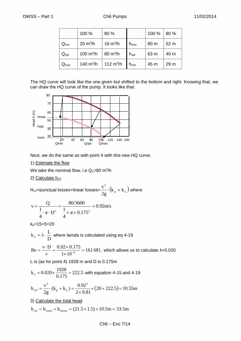
DWSS ndash Part 1 Ch6 Pumps 11022014
Ch6 ndash Exo 714
100 80 100 80
Qmin 20 m3h 16 m3h hmax 80 m 52 m
Qopt 100 m3h 80 m3h hopt 63 m 40 m
Qmax 140 m3h 112 m3h hmin 45 m 29 m
The HQ curve will look like the one given but shifted to the bottom and right Knowing that we can draw the HQ curve of the pump It looks like that
Next we do the same as with point 4 with this new HQ curve
1) Estimate the flow
We take the nominal flow ie Q1=80 m3h
2) Calculate hLP
HLP=punctual losses+linear losses= Lp
2
kk2g
v where
092ms
0175π4
1
803600
Dπ4
1
Qv
22
kp=15+5=20
D
Lλk L where lamda is calculated using eq 4-19
681161101
0175092
ν
DvRe
6
which allows us to calculate λ=0020
L is (as for point 4) 1928 m and D is 0175m
52221750
19280200kL with equation 4-15 and 4-19
m55102225209812
092)k(k
2g
vh
2
Lp
2
LP
3) Calculate the total head
335mm51015)215(hhh lossesstatictot
50
60
70
30
40
Head h
(m
)
120 140 160 80 100 60 40 20
80
Qmin Qopt Qmax
hmin
hopt
hmax
DWSS ndash Part 1 Ch6 Pumps 11022014
Ch6 ndash Exo 814
4) Find a new Q (Q2)
Looking back at the pump characteristics the flow corresponding to a head of 335m is 105m3h This is shown in the following chart As before the purple line is the QP curve given and the blue line is the network characteristics which is the same as the one drawn in point 4
5) Iterate
The average between Q1 (80 m3h) and the flow we obtained at the end Q2 (105 m3h) which gives us a flow of 925 m3h
The iteration are shown in the following table At the end we find a flow of 95 m3h
it Q1 m3h Q m3s v Re lamda kL
stat head
linear loss
Punctual loss
total loss h tot
Q2 m3h
0 80 0022 092 1616812 0020 22250 23 968 087 1055 3355 105
1 925 0026 107 1869439 0020 21984 23 1279 116 1395 3695 97
2 9475 0026 109 1914912 0020 21942 23 1339 122 1461 3761 96
For the power consumption knowing that the flow is 95 m3h and that the power consumption
for this flow is 22 kW we will have 113kW0822n
nPP
3
3
1
212
As it can be noticed the power consumption passes from 26 kW without adjustment to 23kW with a throttling system and to 113 kW with a speed reduction system Compared with a throttling system (where we have almost the same flow reduction) the power consumption with a speed decrease system is much more efficient
9 If the system is working as per exercise 4 what is the maximum suction height And what is the maximum suction height if it is working as in exercise 7
The maximum suction head is when it is equal to the height of the water column minus the head losses in the suction part and the NPSH required by the pump
rS-LPva
suc NPSHhgρ
PPh
At 200 masl the atmospheric pressure is 98 000 Pa (chart chapter 2 page 3) In this exercise we want to avoid cavitation Therefore we have to take the minimum pressure on the chart (light blue line) representing the smallest water column The vapour pressure for water at 20degC is 2340 Pa (figure 2-3)
The height of the water column is mg
PP va 7599811000
234098000
The head losses in the suction part are calculated as follow
40
50
60
20
30
Head H
(m
)
120 140 160 80 100 60 40 20
Q1 Q2 Qduty
DWSS ndash Part 1 Ch6 Pumps 11022014
Ch6 ndash Exo 914
Lp
2
LP kk2g
vh where v=QA and kp=15 (punctual losses in the suction part)
The NPSHr is given in the chart NPSH versus flow
a) When the system is working as per exercise 4
The flow for this system is 130 m3h
The height of the water column is 975m
The head losses in the suction part we have
- kp for the suction part that is 15
- 11850175
10650019
D
LλkL where lambda is from the last iteration of point 6
L=5+15+100=1065 and D is the diameter 0175m
m0831185)(159812
51kk
2g
vh
2
Lp
2
LP
The NPSH For a flow of 130 m3h we find a NPSH of 8 m
Therefore the maximum is 133m8308759hsuc this negative number indicates
clearly that the system designed in point 6 only works if the pump is placed at least 135m below the water level If not cavitation will occur will damage the pump and reduce the flow
b) When the system is working as per exercise 7 (adjustment with a throttling system)
The height of the water column stays at 975m
The head losses in the suction part we have
- kp = 15 for the suction part
- 12070175
10650020
D
LλkL where lamda was recalculated for this flow with eq
419
189m)0712(159812
171kk
2g
vh
2
Lp
2
LP
The NPSH For a flow of 100 m3h we find a NPSH of 6 m
Therefore the maximum is 186m6189759h suc This value being higher than 15 m
(which is the suction height of the pump as it is designed in point 6) indicates that cavitation will not occur with this system
The maximum suction height between point a and b is increased because the flow is decreased which will decrease the head losses and the NPSH required by the pump Thus if we want this system to work without cavitation the flow has to be reduced by throttling trimming or speed reduction
DWSS ndash Part 1 Ch6 Pumps 11022014
Ch6 ndash Exo 1014
Answers to advanced exercises
10 For the system used in exercise 7 (with a throttling system) knowing that the intake water level varies of plus or minus 2 meters what would be the max and min flow what would be the max suction height
a) With plus 2 meters
The flow
We have to do the same iterations as it was done in exercise 4 This time the static head is 21m instead of 23m We can begin the iteration at 100 m3h since the flow will be practically the same (the static head does not change much)
The punctual losses coefficient is equal to the punctual losses in the suction part and delivery part plus the one of the orifice kp=15+5+350=370
it Q
m3h Q
m3s V
ms Re lamba kL
H static
Linear losses
Punctual losses
Total loss h tot
Q2 m3h
0 100 0028 115 2021015 0020 21851 21 1485 2515 4001 6101 1048
1 1024 0028 118 2069280 0020 21813 21 1554 2637 4191 6291 998
2 1011 0028 117 2043199 0020 21833 21 1517 2571 4088 6188 1025
3 1018 0028 118 2057735 0020 21822 21 1538 2607 4145 6245 1010
Thus by decreasing the static head the flow is increased of about 1 Q= 101 m3h
The maximum suction height (for this water level) is calculated as in exercise 9
o the height of the water column is 975 m
o the head losses in the suction part are
921)1750
51060200(15
9812
181
D
Lk
2g
vh
2
p
2
LP
m
o the NPSH is around 6m for a flow of 101 m3h
Therefore the maximum suction height is 975m-192m-6m=184
It must be noticed that it is 184m above the water level for which we calculated the flow which is 2 meters above the average suction level Therefore when the water level is 2m above the
hstat
Minus two meter b
Plus two meters a Average suction level
90
40
50
60
70
80
20
30
Head H
(m
)
120 140 160 80 100 60 40 20 Qa Qb
DWSS ndash Part 1 Ch6 Pumps 11022014
Ch6 ndash Exo 1114
average water level the pump should be placed at a maximum of 384m above the average water level
b) with minus 2 meters
The flow
We have to do the same iterations as it was done before This time the static head is 25m instead of 23m Again we start at a flow of 100 m3h
it Q m3h Q m3s v Re lamda kL
stat head linear loss
punctual loss total loss h tot Q2
0 1000 0028 115 2021015 0020 21851 25 1485 2515 4001 6501 941
1 970 0027 112 1960891 0020 21902 25 1402 2368 3769 6269 1004
2 987 0027 114 1994890 0020 21873 25 1449 2451 3899 6399 969
3 978 0027 113 1976407 0020 21888 25 1423 2405 3828 6328 988
4 983 0027 114 1986684 0020 21880 25 1437 2430 3868 6368 977
5 980 0027 113 1981039 0020 21884 25 1429 2417 3846 6346 983
(The number of iterations necessary to converge on the result has increased because the system curve is steeper which makes the iteration process less efficient)
This time by increasing the static head the flow is decreased of about 2 Q= 98 m3h
The maximum suction height (for this water level) is calculated as before
o the height of the water column is 975 m
o the head losses in the suction part are
m781)1750
51060200(15
9812
131
D
Lk
2g
vh
2
p
2
LP
o the NPSH is around 6m for a flow of 98 m3h
Therefore the maximum suction height is 975m-178m-6m=197m
This height corresponds to a height of 197m above the water level for which we calculated the flow (which is 2 meters below the average suction level) Therefore the pump should be placed just below the average water level or lower (2m-197m=003m=3cm) This level is (not surprisingly) lower than the one obtained in a Therefore this is the value to be considered when doing the design to find the elevation of the pump avoiding cavitation As a result if the pump is place 15 m above the surface level (as it is the case in exercise 7) it will cavitate when the water level will drop down As it can be seen the variation of the water level in the intake tank has a big impact on cavitation and should be taken into account when doing calculations
11 With a frequency inverter what should be the percent speed reduction to adjust the system to the nominal point of the pump What is the corresponding flow
As it is explained in the section about speed reduction the line of nominal points with a speed reduction is parable In order to find the point where the system is at its nominal point we will have to find the place where the nominal point line crosses the system curve This is shown on the following graph
DWSS ndash Part 1 Ch6 Pumps 11022014
Ch6 ndash Exo 1214
0
20
40
60
80
100
120
140
0 50 100 150
Flow (m3h)
Head
(m
)
System curve
Line of nominal point
Pump curve w ithout speed
reduction
Pump curve w ith x speed
reduction
First we have to find the equation of this parable A parable is from the type
y=ax2+bx+c In our case it is hn=aQn2+bQn+c (hn and Qn indicates the nominal head and
nominal flow respectively)
We know that it passes by the origin thus c=0 Therefore the equation of the parable will be from the type
hn=aQn2+bQn
To find the coefficient a and b we need two points on this curve
If we do not change the system the nominal point is Qn=100 m3h and hn=63 which will be the first of the two needed points
The second point (which is whichever point on the curve with r rotation speed) will have apostrophe (Hn and Qn) to make the difference between the first (with 100 speed) and second point (r speed)
2
n
n
n
n
n
2
n
n
n
2
nn
rhh(4)
rQQ(3)
QbQah(2)
QbQah(1)
Substituting (3) and (4) into (2) we get
rbQraQrh)5( n
22
n
2
n
which simplifies to (dividing by r)
n
2
nn bQraQrh(6)
From (1) we know that
2
nnn QahQb)7(
Putting (7) back into (6) we get
2
nn
2
nn QahrQarh)8(
DWSS ndash Part 1 Ch6 Pumps 11022014
Ch6 ndash Exo 1314
which can be written as
1)(rQa1)(rh)9( 2
nn
If follows that
2
n
n
Q
ha)10( In that case given that Qn=100 m3h and hn=63 we have 30006
100
63a
2
To find the coefficient b we use (10) and (1) and find
n
2
n2
n
nn QbQ
Q
hh)11(
which gives us b=0
Therefore our equation of the line of nominal point is 200063Qh
To find the intersection of the line of nominal point and the system curve we will have to iterate in a slightly different way as before
For a given flow Q1 we will estimate the losses and the total head (static head plus head losses) as it was done before
Then for this head we will find the corresponding flow Q2 on the line of nominal points To find the nominal flow for a given head we solve the following equation for Q
0h00063Q2 which gives us 00063
hQ
This time Q2 can directly be taken for the next iteration (no need to do the average between Q1 and Q2) This is because between Q1 and Q2 we do not cross the intersection as it was the case for the previous iterations (this can be seen in the following figure) Therefore we get closer to the results every time and Q2 can be taken for the next iteration
We will start the iteration at the nominal flow without speed reduction system namely 100 m3h The iterations are shown in the following table
0
20
40
60
80
100
120
140
0 50 100 150
System curve Line of nominal point
Q1 Q2
DWSS ndash Part 1 Ch6 Pumps 11022014
Ch6 ndash Exo 1414
it Q m3h
Q m3s v Re lamda kL
stat head
linear loss
punctual loss
total loss total h Q2
0 100 0028 115 202102 002 21851 23 148538 13595 162134 3921 789
1 7889 0022 091 159447 002 22277 23 942562 08462 102718 3327 727
2 7267 002 084 146872 002 22441 23 805645 0718 877446 3177 71
3 7102 002 082 143529 002 22489 23 771023 06857 839593 314 706
4 7059 002 082 142671 002 22501 23 762262 06775 830015 313 705
At the end we get approximately a flow of 70 m3h
Given that 1
2
1
2
n
n
Q
Q and that we have 07
100
70
Q
Q
1
2 it follows that 07n
n
1
2
Therefore the speed reduction should be of 70
For the pump a we have a frequency of 50 Hz Given that the rotation speed is directly proportional to the frequency the frequency will have to be reduced to 70 of its initial value which is 35 Hz
DWSS ndash Part 1 Ch7 Water hammer 11022014
Ch7 ndash Exo 17
Answers to basic exercises
1 Draw the pressure and the velocity versus the time (Lc) at the middle of the pipe for an instantaneous valve closure neglecting head losses
The surge will arrive at the middle of the pipe after half of the time needed to travel the pipe L2c and come back after two times this time 2L2c=Lc
2 What are the velocity of the pressure wave (c) the head surge (Δh) and the return time in a cast iron pipe DN200 of 3 kilometres for a instantaneous decrease of velocity of 15 ms
With the table of Cast iron pipe in the annexe N we find with DN200 the value of c=1216 ms To find Δh we have to multiple the given value by the actual velocity Δh=124times15=186 m To find the return time we have to multiple the given value by the actual length in km Tr=16times3=48 s
In this case the pressure surge is huge (almost 18 bar) but the return time very short thus if it is possible to extend the closure or stopping time to 10 s the surge would be divided by 2 (9 bar) and with 20 s by 4 (ie 45 bar)
3 What are the velocity of the pressure wave (c) the head surge (Δh) and the return time in a PE pipe SDR11 of 5 kilometres for a instantaneous decrease of velocity of 2 ms
With the table of PE pipe in the annexe N we find with SDR11 (the diameter of the pipe is not needed the water hammer will be the same for the all series) the value of c=342 ms To find Δh we have to multiple the given value by the actual velocity Δh=35times2=70 m To find the return time we have to multiple the given value by the actual length in km Tr=58times5=29 s
In this case we can see that the pressure surge is smaller (~7 bar) but that the return time is quite important almost half minute before the surge is back
4 What are the velocity of the pressure wave (c) the head surge (Δh) and the return time in a PVC pipe SDR17 OD 200 of 2 kilometres for a instantaneous closure with an initial velocity of 1 ms
With the table of PVC pipe ODgt100 in the annexe N we find with SDR17 (the water hammer will be the same for the all series with ODgt100) the value of c=490 ms The Δh is the one in the table as the velocity is of 1 ms Δh=50 m To find the return time we have to multiple the given value by the actual length in km Tr=41times2=82 s
In this case we can see that the pressure surge is quite small (~5 bar) and the return time not too long (less than 10 s) Thus this pipe should be not too much at risk
pre
ssure
time
L2c
-ΔP
P0
t0 Lc 2Lc 3Lc 4Lc
+Δ
P
1 2
5Lc
3 4 Phases
t0
Reversed flow
Ve
locity
v0
Lc Lc
time Lc 2Lc 3Lc 4Lc 5Lc
DWSS ndash Part 1 Ch7 Water hammer 11022014
Ch7 ndash Exo 27
5 What length of the previous pipe will have a reduced surge if the closure time is of 41 second
The length with reduce surge is according to eq 74 is Lred = Tc c 2 = 41 times 490 2 = 1000 m Thus with a decreasing time of half the return time half of the pipeline will have reduced pressure durge
6 Neglecting losses draw the envelope scheme for the previous pipe knowing that its profile is as per the attached table Is the pipe safe (assuming a linear front wave) If not what can be done
Pump Pt 1 Pt 2 Pt 3 Tank
Pipe length 0 500 1000 1500 2000
Elevation 0 10 30 30 70
We can see that a part of the pipeline (between 750 and 1 200) will be exposed to depressure and that around 1 000 m it might even face cavitation There is no risk of pipe burst (over pressure) as the maximum pressure (hstat + Δh = 120) is smaller than the pipe PN (~125 m) In order to avoid this depressure in the pipe the following could be done - Increase the stopping time - Install air valves letting air come into the pipe in the zone at risk
7 For the previous system what should be the closure time to limit the Δh at 30m
According to Eq 75 s61330819
120002
hg
v2LT
Tg
v2Lh
max
inc
c
inmax
Thus to reduce the Δh to 30 m the closure time should be of 136 s In theory this would be also valid for a cast iron pipe or any material with a return time for this system smaller than 136 s
Δh=50m
Static line
Lred = 1 000 m
Zone at risk
Min acceptable pressure
Max acceptable pressure
Δh=50m
500 1 000 1 500 2 000
70
30
10
120 125
Pipe length [m]
Elevation [m]
-8
DWSS ndash Part 1 Ch7 Water hammer 11022014
Ch7 ndash Exo 37
Answers to intermediary exercises
8 Draw the pressure and the velocity versus the time (Lc) at the middle of the pipe for an instantaneous valve closure taking into consideration head losses
The surge will arrive at the middle of the pipe after half of the time needed to travel the pipe L2c and come back after two times this time 2L2c=Lc
9 What are the velocity (c) the head surge (Δh) and the return time (Tr) of the pressure wave in a cast iron pipe DN200 (e=64 mm Kpipe=140 GPa) of 3 km if a pump of 170 m3h instantaneously stops working with a temperature of water of 45deg
We calculate c with Eq 7-1
pipe
water
water
K
K
e
D1
ρKc
where at 45deg Kwater is 229 GPa and ρ=9902 kgm3
The thickness e is 64 mm KCI is 140 GPa
The diameter D can be estimated as the nominal diameter (DN) so 200 mm
so ms 1237
10140
10229
64
2001
990210229
K
K
e
D1
ρKc
9
9
9
pipe
water
water
Given that the flow is totally stopped
ms 150
102004
π
1703600
A
QvΔv
23
The head surge is found with equation 7-1 Δh = Δvmiddotcg=15 times 1237 981 = 1896 m
The return time is found with equation 7-3 Tr= 2Lc= 2 times 3000 1237 = 485 s
If we compare these results with the exercise 2 we can see that they are very close the difference of taking in to consideration the water temperature of 45deg make a difference of 15 on the head surge and of 1 on the return time
pre
ssure
time
L2c
-ΔP
P0
t0 Lc 2Lc 3Lc 4Lc
+Δ
P
1 2
5Lc
3 4 Phases
t0
Reversed flow
Ve
locity
v0
Lc Lc
time Lc 2Lc 3Lc 4Lc 5Lc
DWSS ndash Part 1 Ch7 Water hammer 11022014
Ch7 ndash Exo 47
10 For the previous pipe we want to limit the head surge at 100m by having a longer stopping time what should be in this case TC
According to equation 7-5 we have s 179100819
5130002
hg
v2LT
max
inc
BY increasing significantly the closure time we will have almost half of the flow when the head surge is coming back therefore the Δv is divided by two dividing thus also the head surge by two
11 What are the velocity (c) the head surge (Δh) and the return time (Tr) of the pressure wave in a PE80 pipe PN125 OD200 (KPE=07 GPa e=182mm) of 5 km if a pump of 150 m3h instantaneously stops working with a temperature of water of 20deg
We calculate c with Eq 7-1
pipe
water
water
K
K
e
D1
ρKc
where at 20deg Kwater is 22 GPa and ρ=9982 kgm3
The nominal thickness for this pipe is given 182 mm (an average of 192 could be used)
The bulk modulus KPE is given as 07 GPa
The internal diameter D is thus per Annexe B 1636 mm
so ms 742
1070
1022
182
16361
99821022
K
K
e
D1
ρKc
9
9
9
pipe
water
water
Given that the flow is totally stopped
ms 1982
102004
π
1503600
A
QvΔv
23
The head surge is found with equation 7-1 Δh = Δvmiddotcg=1982 times 274 981 = 555 m
The return time is found with equation 7-3 Tr= 2Lc= 2 times 5000 274 = 364 s
This time if we compare these results with the exercise 3 we can see that they are not so close as the bulk modulus given is quite different from the one used in the table in annexe N
12 What are the friction coefficient (KLP) and the head losses (hLP) of the previous pipe with a roughness of 007 mm neglecting the punctual losses What is the attenuation of the negative head surge due to the losses at the tank
With equation 4-9 we find Re = D middot v ν = 1636 times 1982 101 times 10-6 = 322 000
With equation 4-19 or fig 4-5 we find λ = 00147
As the singular losses are neglected we find with equations 4-15
KLP = λ middot L D = 00147 times 5 000 01636 = 449
hLP = v2 middot λ 2g = 19822 times 449 (2 times 981) = 899 m
Thus the attenuation of the negative head surge at the tank is equal to hlosses2 about 45m In this situation where the losses are quite high as the velocity is important we can see that the remaining negative head surge at the tank is only of 10m thus the importance to take them in to account
DWSS ndash Part 1 Ch7 Water hammer 11022014
Ch7 ndash Exo 57
13 What are the attenuation of head surge at the valve (hv-att) the remaining velocity at the tank (vt1) and the attenuation of the positive head surge at the tank (ht-att) of the previous pipe
With equation 7-6 we find m 8254499812
7421-274
982144921
2gk
c1-c
vk21
h
2
2
LP
2
2
inLP
att-v
With equation 4-9 we find
m 52494981
7421-274
6071982149412
gk
c1-c
vvk12
h
ms 60712744
9821449
4c
vkv
2
2
LP
2
2
t1inLP
att-t
22
inLPt1
Thus when the surge arrive to the tank the velocity in the depression zone reaches 1607 ms This explains why the negative head surge is so small at the tanks as the difference of velocity is then only of 1982-1602=0375 ms
The attenuation of the positive head surge at the valve is of 258 m thus the positive head surge at the valve is of 555 - 258 asymp 30 m NB this value as to be added at the static level not at the dynamic one This value is much smaller than the initial head losses (899 m) thus the positive head surge is not affecting the pipe at the valve
The attenuation of the positive head surge at the tank is of 25 m thus the positive head surge at the tank is of 555 ndash 899 2 ndash 25 asymp 8 m This remaining positive head surge at the tank is very small
See the next exercise correction for an illustration of these results
14 For the previous pipe draw the developed profile of the pipeline the static and dynamic lines and the envelope schemes knowing that its profile is as per the attached table Is the pipe safe If not what can be done
Pump Pt 1 Pt 2 Pt 3 Tank
Pipe length 0 1000 1000 1000 2000
Elevation 0 0 5 10 30
As explain in the section 76 the developed profile should be used but as the slopes are small it doesnt make a big difference if it is taken into consideration or not
All the values calculated in the previous exercises were reported in this chart
It can be seen that the superior envelope is much lower than the maximum acceptable pressure thus there is no risk of pipe burst in case of water hammer
However the inferior level is lower than the ground level even lower than the cavitation line (minimum acceptable pressure) thus depressure and cavitation will happen in this pipeline if it is not protected
Possible solutions might include a pump bypass system or air valve Nevertheless into this situation the best would be to increase the diameter of the pipe decreasing also the losses and necessary PN for the pipe this will thus decrease the thickness and further the head surge
DWSS ndash Part 1 Ch7 Water hammer 11022014
Ch7 ndash Exo 67
15 What would be the effect on the head surge on the previous exercises of having a Youngs modulus (KPE)of 11 GPa instead of 07 GPa
The surge velocity will be at 341 ms instead of 274 ms increasing the head surge at 70 m instead of 56 m This will significantly increase the problematic of the depressure at the valve even for bigger diameters This shows the importance to have a good information from the supplier about the properties of the pipes and in case of doubt to take a good margin between the envelope and the maximum or minimum tolerable pressure
16 For exercise 2-4 what would be the change in ID (DN for metallic pipe) following the change in pressure due to water hammer
In order to calculate ΔD we use a formula from chapter 1 (Eq 1-5)
2e
D
K
ΔPDΔD
K is the Youngs modulus of the pipe material For the first exercise to find ΔD in mm we have
0026mm642
200
10125
1053400200ΔD
9
Therefore when the pipe will be in overpressure the DN will be Do=200+0026=200026 mm (the pipe will be expanded)
When the pipe will be in under pressure the DN will be Du= 200-0026=19997
Answers to advanced exercises
11m
Developed profile of the pipeline
-30
-10
10
30
50
70
90
110
130
0 500 1000 1500 2000 2500 3000 3500 4000 4500 5000
Dynamic or piezo line
Static line
Overpressure envelope
Depressure envelope
Pipeline
Min acceptable pressure
Max acceptable pressure
0
Elevation
PN
of
the p
ie ~
123m
Head losses
~90m
Attenuated positive head surge at the
valve ~30m
Tank elevation
~30m
Depressure ~56m
Pipe length [m]
Cavitation ~9m Head losses2
~45m
Attenuation of head surge at the valve
~26m Head losses2 +
ht-att ~48m
8m
DWSS ndash Part 1 Ch7 Water hammer 11022014
Ch7 ndash Exo 77
The same procedure is done for exercise 3 amp 4 The results are shown it the following table
Ex ΔP Pa DN or ID mm e mm K GPa ΔD mm Do mm Du mm
2
3
4
We can draw the following conclusion
even if the ΔP is bigger for cast iron the change in diameter will be less than for PE (because PE is easily distorted)
even if the ΔP is bigger for exercise 4 than for 3 the change in pipes diameter will be bigger for 3 because the wall thickness is smaller (which makes the pipe more easily distorted)
It can be noticed that the expansion due to changes in pressure in the pipe is not significant because even for PE pipe with a bigger expansion it is around half a millimetre added to the outside diameter which is less than the tolerance margin for PE pipe For example for a PE pipe having an OD of 200 mm the maximum outside diameter will be of 2012 mm (which is bigger than 2005 obtained with pressure expansion) These calculations were done for expansion due to pressure changes only because of water hammer (thus ignoring the initial pressure in the pipe) This means that the diameter can be more expanded because the total change in pressure will be bigger Furthermore if we have an initial pressure it must be checked that the PN of the pipe can bear the total pressure (initial pressure +ΔP)
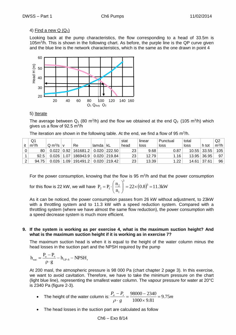
DWSS ndash Part 1 Ch6 Pumps 11022014
Ch6 ndash Exo 1414
it Q m3h
Q m3s v Re lamda kL
stat head
linear loss
punctual loss
total loss total h Q2
0 100 0028 115 202102 002 21851 23 148538 13595 162134 3921 789
1 7889 0022 091 159447 002 22277 23 942562 08462 102718 3327 727
2 7267 002 084 146872 002 22441 23 805645 0718 877446 3177 71
3 7102 002 082 143529 002 22489 23 771023 06857 839593 314 706
4 7059 002 082 142671 002 22501 23 762262 06775 830015 313 705
At the end we get approximately a flow of 70 m3h
Given that 1
2
1
2
n
n
Q
Q and that we have 07
100
70
Q
Q
1
2 it follows that 07n
n
1
2
Therefore the speed reduction should be of 70
For the pump a we have a frequency of 50 Hz Given that the rotation speed is directly proportional to the frequency the frequency will have to be reduced to 70 of its initial value which is 35 Hz
DWSS ndash Part 1 Ch7 Water hammer 11022014
Ch7 ndash Exo 17
Answers to basic exercises
1 Draw the pressure and the velocity versus the time (Lc) at the middle of the pipe for an instantaneous valve closure neglecting head losses
The surge will arrive at the middle of the pipe after half of the time needed to travel the pipe L2c and come back after two times this time 2L2c=Lc
2 What are the velocity of the pressure wave (c) the head surge (Δh) and the return time in a cast iron pipe DN200 of 3 kilometres for a instantaneous decrease of velocity of 15 ms
With the table of Cast iron pipe in the annexe N we find with DN200 the value of c=1216 ms To find Δh we have to multiple the given value by the actual velocity Δh=124times15=186 m To find the return time we have to multiple the given value by the actual length in km Tr=16times3=48 s
In this case the pressure surge is huge (almost 18 bar) but the return time very short thus if it is possible to extend the closure or stopping time to 10 s the surge would be divided by 2 (9 bar) and with 20 s by 4 (ie 45 bar)
3 What are the velocity of the pressure wave (c) the head surge (Δh) and the return time in a PE pipe SDR11 of 5 kilometres for a instantaneous decrease of velocity of 2 ms
With the table of PE pipe in the annexe N we find with SDR11 (the diameter of the pipe is not needed the water hammer will be the same for the all series) the value of c=342 ms To find Δh we have to multiple the given value by the actual velocity Δh=35times2=70 m To find the return time we have to multiple the given value by the actual length in km Tr=58times5=29 s
In this case we can see that the pressure surge is smaller (~7 bar) but that the return time is quite important almost half minute before the surge is back
4 What are the velocity of the pressure wave (c) the head surge (Δh) and the return time in a PVC pipe SDR17 OD 200 of 2 kilometres for a instantaneous closure with an initial velocity of 1 ms
With the table of PVC pipe ODgt100 in the annexe N we find with SDR17 (the water hammer will be the same for the all series with ODgt100) the value of c=490 ms The Δh is the one in the table as the velocity is of 1 ms Δh=50 m To find the return time we have to multiple the given value by the actual length in km Tr=41times2=82 s
In this case we can see that the pressure surge is quite small (~5 bar) and the return time not too long (less than 10 s) Thus this pipe should be not too much at risk
pre
ssure
time
L2c
-ΔP
P0
t0 Lc 2Lc 3Lc 4Lc
+Δ
P
1 2
5Lc
3 4 Phases
t0
Reversed flow
Ve
locity
v0
Lc Lc
time Lc 2Lc 3Lc 4Lc 5Lc
DWSS ndash Part 1 Ch7 Water hammer 11022014
Ch7 ndash Exo 27
5 What length of the previous pipe will have a reduced surge if the closure time is of 41 second
The length with reduce surge is according to eq 74 is Lred = Tc c 2 = 41 times 490 2 = 1000 m Thus with a decreasing time of half the return time half of the pipeline will have reduced pressure durge
6 Neglecting losses draw the envelope scheme for the previous pipe knowing that its profile is as per the attached table Is the pipe safe (assuming a linear front wave) If not what can be done
Pump Pt 1 Pt 2 Pt 3 Tank
Pipe length 0 500 1000 1500 2000
Elevation 0 10 30 30 70
We can see that a part of the pipeline (between 750 and 1 200) will be exposed to depressure and that around 1 000 m it might even face cavitation There is no risk of pipe burst (over pressure) as the maximum pressure (hstat + Δh = 120) is smaller than the pipe PN (~125 m) In order to avoid this depressure in the pipe the following could be done - Increase the stopping time - Install air valves letting air come into the pipe in the zone at risk
7 For the previous system what should be the closure time to limit the Δh at 30m
According to Eq 75 s61330819
120002
hg
v2LT
Tg
v2Lh
max
inc
c
inmax
Thus to reduce the Δh to 30 m the closure time should be of 136 s In theory this would be also valid for a cast iron pipe or any material with a return time for this system smaller than 136 s
Δh=50m
Static line
Lred = 1 000 m
Zone at risk
Min acceptable pressure
Max acceptable pressure
Δh=50m
500 1 000 1 500 2 000
70
30
10
120 125
Pipe length [m]
Elevation [m]
-8
DWSS ndash Part 1 Ch7 Water hammer 11022014
Ch7 ndash Exo 37
Answers to intermediary exercises
8 Draw the pressure and the velocity versus the time (Lc) at the middle of the pipe for an instantaneous valve closure taking into consideration head losses
The surge will arrive at the middle of the pipe after half of the time needed to travel the pipe L2c and come back after two times this time 2L2c=Lc
9 What are the velocity (c) the head surge (Δh) and the return time (Tr) of the pressure wave in a cast iron pipe DN200 (e=64 mm Kpipe=140 GPa) of 3 km if a pump of 170 m3h instantaneously stops working with a temperature of water of 45deg
We calculate c with Eq 7-1
pipe
water
water
K
K
e
D1
ρKc
where at 45deg Kwater is 229 GPa and ρ=9902 kgm3
The thickness e is 64 mm KCI is 140 GPa
The diameter D can be estimated as the nominal diameter (DN) so 200 mm
so ms 1237
10140
10229
64
2001
990210229
K
K
e
D1
ρKc
9
9
9
pipe
water
water
Given that the flow is totally stopped
ms 150
102004
π
1703600
A
QvΔv
23
The head surge is found with equation 7-1 Δh = Δvmiddotcg=15 times 1237 981 = 1896 m
The return time is found with equation 7-3 Tr= 2Lc= 2 times 3000 1237 = 485 s
If we compare these results with the exercise 2 we can see that they are very close the difference of taking in to consideration the water temperature of 45deg make a difference of 15 on the head surge and of 1 on the return time
pre
ssure
time
L2c
-ΔP
P0
t0 Lc 2Lc 3Lc 4Lc
+Δ
P
1 2
5Lc
3 4 Phases
t0
Reversed flow
Ve
locity
v0
Lc Lc
time Lc 2Lc 3Lc 4Lc 5Lc
DWSS ndash Part 1 Ch7 Water hammer 11022014
Ch7 ndash Exo 47
10 For the previous pipe we want to limit the head surge at 100m by having a longer stopping time what should be in this case TC
According to equation 7-5 we have s 179100819
5130002
hg
v2LT
max
inc
BY increasing significantly the closure time we will have almost half of the flow when the head surge is coming back therefore the Δv is divided by two dividing thus also the head surge by two
11 What are the velocity (c) the head surge (Δh) and the return time (Tr) of the pressure wave in a PE80 pipe PN125 OD200 (KPE=07 GPa e=182mm) of 5 km if a pump of 150 m3h instantaneously stops working with a temperature of water of 20deg
We calculate c with Eq 7-1
pipe
water
water
K
K
e
D1
ρKc
where at 20deg Kwater is 22 GPa and ρ=9982 kgm3
The nominal thickness for this pipe is given 182 mm (an average of 192 could be used)
The bulk modulus KPE is given as 07 GPa
The internal diameter D is thus per Annexe B 1636 mm
so ms 742
1070
1022
182
16361
99821022
K
K
e
D1
ρKc
9
9
9
pipe
water
water
Given that the flow is totally stopped
ms 1982
102004
π
1503600
A
QvΔv
23
The head surge is found with equation 7-1 Δh = Δvmiddotcg=1982 times 274 981 = 555 m
The return time is found with equation 7-3 Tr= 2Lc= 2 times 5000 274 = 364 s
This time if we compare these results with the exercise 3 we can see that they are not so close as the bulk modulus given is quite different from the one used in the table in annexe N
12 What are the friction coefficient (KLP) and the head losses (hLP) of the previous pipe with a roughness of 007 mm neglecting the punctual losses What is the attenuation of the negative head surge due to the losses at the tank
With equation 4-9 we find Re = D middot v ν = 1636 times 1982 101 times 10-6 = 322 000
With equation 4-19 or fig 4-5 we find λ = 00147
As the singular losses are neglected we find with equations 4-15
KLP = λ middot L D = 00147 times 5 000 01636 = 449
hLP = v2 middot λ 2g = 19822 times 449 (2 times 981) = 899 m
Thus the attenuation of the negative head surge at the tank is equal to hlosses2 about 45m In this situation where the losses are quite high as the velocity is important we can see that the remaining negative head surge at the tank is only of 10m thus the importance to take them in to account
DWSS ndash Part 1 Ch7 Water hammer 11022014
Ch7 ndash Exo 57
13 What are the attenuation of head surge at the valve (hv-att) the remaining velocity at the tank (vt1) and the attenuation of the positive head surge at the tank (ht-att) of the previous pipe
With equation 7-6 we find m 8254499812
7421-274
982144921
2gk
c1-c
vk21
h
2
2
LP
2
2
inLP
att-v
With equation 4-9 we find
m 52494981
7421-274
6071982149412
gk
c1-c
vvk12
h
ms 60712744
9821449
4c
vkv
2
2
LP
2
2
t1inLP
att-t
22
inLPt1
Thus when the surge arrive to the tank the velocity in the depression zone reaches 1607 ms This explains why the negative head surge is so small at the tanks as the difference of velocity is then only of 1982-1602=0375 ms
The attenuation of the positive head surge at the valve is of 258 m thus the positive head surge at the valve is of 555 - 258 asymp 30 m NB this value as to be added at the static level not at the dynamic one This value is much smaller than the initial head losses (899 m) thus the positive head surge is not affecting the pipe at the valve
The attenuation of the positive head surge at the tank is of 25 m thus the positive head surge at the tank is of 555 ndash 899 2 ndash 25 asymp 8 m This remaining positive head surge at the tank is very small
See the next exercise correction for an illustration of these results
14 For the previous pipe draw the developed profile of the pipeline the static and dynamic lines and the envelope schemes knowing that its profile is as per the attached table Is the pipe safe If not what can be done
Pump Pt 1 Pt 2 Pt 3 Tank
Pipe length 0 1000 1000 1000 2000
Elevation 0 0 5 10 30
As explain in the section 76 the developed profile should be used but as the slopes are small it doesnt make a big difference if it is taken into consideration or not
All the values calculated in the previous exercises were reported in this chart
It can be seen that the superior envelope is much lower than the maximum acceptable pressure thus there is no risk of pipe burst in case of water hammer
However the inferior level is lower than the ground level even lower than the cavitation line (minimum acceptable pressure) thus depressure and cavitation will happen in this pipeline if it is not protected
Possible solutions might include a pump bypass system or air valve Nevertheless into this situation the best would be to increase the diameter of the pipe decreasing also the losses and necessary PN for the pipe this will thus decrease the thickness and further the head surge
DWSS ndash Part 1 Ch7 Water hammer 11022014
Ch7 ndash Exo 67
15 What would be the effect on the head surge on the previous exercises of having a Youngs modulus (KPE)of 11 GPa instead of 07 GPa
The surge velocity will be at 341 ms instead of 274 ms increasing the head surge at 70 m instead of 56 m This will significantly increase the problematic of the depressure at the valve even for bigger diameters This shows the importance to have a good information from the supplier about the properties of the pipes and in case of doubt to take a good margin between the envelope and the maximum or minimum tolerable pressure
16 For exercise 2-4 what would be the change in ID (DN for metallic pipe) following the change in pressure due to water hammer
In order to calculate ΔD we use a formula from chapter 1 (Eq 1-5)
2e
D
K
ΔPDΔD
K is the Youngs modulus of the pipe material For the first exercise to find ΔD in mm we have
0026mm642
200
10125
1053400200ΔD
9
Therefore when the pipe will be in overpressure the DN will be Do=200+0026=200026 mm (the pipe will be expanded)
When the pipe will be in under pressure the DN will be Du= 200-0026=19997
Answers to advanced exercises
11m
Developed profile of the pipeline
-30
-10
10
30
50
70
90
110
130
0 500 1000 1500 2000 2500 3000 3500 4000 4500 5000
Dynamic or piezo line
Static line
Overpressure envelope
Depressure envelope
Pipeline
Min acceptable pressure
Max acceptable pressure
0
Elevation
PN
of
the p
ie ~
123m
Head losses
~90m
Attenuated positive head surge at the
valve ~30m
Tank elevation
~30m
Depressure ~56m
Pipe length [m]
Cavitation ~9m Head losses2
~45m
Attenuation of head surge at the valve
~26m Head losses2 +
ht-att ~48m
8m
DWSS ndash Part 1 Ch7 Water hammer 11022014
Ch7 ndash Exo 77
The same procedure is done for exercise 3 amp 4 The results are shown it the following table
Ex ΔP Pa DN or ID mm e mm K GPa ΔD mm Do mm Du mm
2
3
4
We can draw the following conclusion
even if the ΔP is bigger for cast iron the change in diameter will be less than for PE (because PE is easily distorted)
even if the ΔP is bigger for exercise 4 than for 3 the change in pipes diameter will be bigger for 3 because the wall thickness is smaller (which makes the pipe more easily distorted)
It can be noticed that the expansion due to changes in pressure in the pipe is not significant because even for PE pipe with a bigger expansion it is around half a millimetre added to the outside diameter which is less than the tolerance margin for PE pipe For example for a PE pipe having an OD of 200 mm the maximum outside diameter will be of 2012 mm (which is bigger than 2005 obtained with pressure expansion) These calculations were done for expansion due to pressure changes only because of water hammer (thus ignoring the initial pressure in the pipe) This means that the diameter can be more expanded because the total change in pressure will be bigger Furthermore if we have an initial pressure it must be checked that the PN of the pipe can bear the total pressure (initial pressure +ΔP)

DWSS ndash Part 1 Ch7 Water hammer 11022014
Ch7 ndash Exo 17
Answers to basic exercises
1 Draw the pressure and the velocity versus the time (Lc) at the middle of the pipe for an instantaneous valve closure neglecting head losses
The surge will arrive at the middle of the pipe after half of the time needed to travel the pipe L2c and come back after two times this time 2L2c=Lc
2 What are the velocity of the pressure wave (c) the head surge (Δh) and the return time in a cast iron pipe DN200 of 3 kilometres for a instantaneous decrease of velocity of 15 ms
With the table of Cast iron pipe in the annexe N we find with DN200 the value of c=1216 ms To find Δh we have to multiple the given value by the actual velocity Δh=124times15=186 m To find the return time we have to multiple the given value by the actual length in km Tr=16times3=48 s
In this case the pressure surge is huge (almost 18 bar) but the return time very short thus if it is possible to extend the closure or stopping time to 10 s the surge would be divided by 2 (9 bar) and with 20 s by 4 (ie 45 bar)
3 What are the velocity of the pressure wave (c) the head surge (Δh) and the return time in a PE pipe SDR11 of 5 kilometres for a instantaneous decrease of velocity of 2 ms
With the table of PE pipe in the annexe N we find with SDR11 (the diameter of the pipe is not needed the water hammer will be the same for the all series) the value of c=342 ms To find Δh we have to multiple the given value by the actual velocity Δh=35times2=70 m To find the return time we have to multiple the given value by the actual length in km Tr=58times5=29 s
In this case we can see that the pressure surge is smaller (~7 bar) but that the return time is quite important almost half minute before the surge is back
4 What are the velocity of the pressure wave (c) the head surge (Δh) and the return time in a PVC pipe SDR17 OD 200 of 2 kilometres for a instantaneous closure with an initial velocity of 1 ms
With the table of PVC pipe ODgt100 in the annexe N we find with SDR17 (the water hammer will be the same for the all series with ODgt100) the value of c=490 ms The Δh is the one in the table as the velocity is of 1 ms Δh=50 m To find the return time we have to multiple the given value by the actual length in km Tr=41times2=82 s
In this case we can see that the pressure surge is quite small (~5 bar) and the return time not too long (less than 10 s) Thus this pipe should be not too much at risk
pre
ssure
time
L2c
-ΔP
P0
t0 Lc 2Lc 3Lc 4Lc
+Δ
P
1 2
5Lc
3 4 Phases
t0
Reversed flow
Ve
locity
v0
Lc Lc
time Lc 2Lc 3Lc 4Lc 5Lc
DWSS ndash Part 1 Ch7 Water hammer 11022014
Ch7 ndash Exo 27
5 What length of the previous pipe will have a reduced surge if the closure time is of 41 second
The length with reduce surge is according to eq 74 is Lred = Tc c 2 = 41 times 490 2 = 1000 m Thus with a decreasing time of half the return time half of the pipeline will have reduced pressure durge
6 Neglecting losses draw the envelope scheme for the previous pipe knowing that its profile is as per the attached table Is the pipe safe (assuming a linear front wave) If not what can be done
Pump Pt 1 Pt 2 Pt 3 Tank
Pipe length 0 500 1000 1500 2000
Elevation 0 10 30 30 70
We can see that a part of the pipeline (between 750 and 1 200) will be exposed to depressure and that around 1 000 m it might even face cavitation There is no risk of pipe burst (over pressure) as the maximum pressure (hstat + Δh = 120) is smaller than the pipe PN (~125 m) In order to avoid this depressure in the pipe the following could be done - Increase the stopping time - Install air valves letting air come into the pipe in the zone at risk
7 For the previous system what should be the closure time to limit the Δh at 30m
According to Eq 75 s61330819
120002
hg
v2LT
Tg
v2Lh
max
inc
c
inmax
Thus to reduce the Δh to 30 m the closure time should be of 136 s In theory this would be also valid for a cast iron pipe or any material with a return time for this system smaller than 136 s
Δh=50m
Static line
Lred = 1 000 m
Zone at risk
Min acceptable pressure
Max acceptable pressure
Δh=50m
500 1 000 1 500 2 000
70
30
10
120 125
Pipe length [m]
Elevation [m]
-8
DWSS ndash Part 1 Ch7 Water hammer 11022014
Ch7 ndash Exo 37
Answers to intermediary exercises
8 Draw the pressure and the velocity versus the time (Lc) at the middle of the pipe for an instantaneous valve closure taking into consideration head losses
The surge will arrive at the middle of the pipe after half of the time needed to travel the pipe L2c and come back after two times this time 2L2c=Lc
9 What are the velocity (c) the head surge (Δh) and the return time (Tr) of the pressure wave in a cast iron pipe DN200 (e=64 mm Kpipe=140 GPa) of 3 km if a pump of 170 m3h instantaneously stops working with a temperature of water of 45deg
We calculate c with Eq 7-1
pipe
water
water
K
K
e
D1
ρKc
where at 45deg Kwater is 229 GPa and ρ=9902 kgm3
The thickness e is 64 mm KCI is 140 GPa
The diameter D can be estimated as the nominal diameter (DN) so 200 mm
so ms 1237
10140
10229
64
2001
990210229
K
K
e
D1
ρKc
9
9
9
pipe
water
water
Given that the flow is totally stopped
ms 150
102004
π
1703600
A
QvΔv
23
The head surge is found with equation 7-1 Δh = Δvmiddotcg=15 times 1237 981 = 1896 m
The return time is found with equation 7-3 Tr= 2Lc= 2 times 3000 1237 = 485 s
If we compare these results with the exercise 2 we can see that they are very close the difference of taking in to consideration the water temperature of 45deg make a difference of 15 on the head surge and of 1 on the return time
pre
ssure
time
L2c
-ΔP
P0
t0 Lc 2Lc 3Lc 4Lc
+Δ
P
1 2
5Lc
3 4 Phases
t0
Reversed flow
Ve
locity
v0
Lc Lc
time Lc 2Lc 3Lc 4Lc 5Lc
DWSS ndash Part 1 Ch7 Water hammer 11022014
Ch7 ndash Exo 47
10 For the previous pipe we want to limit the head surge at 100m by having a longer stopping time what should be in this case TC
According to equation 7-5 we have s 179100819
5130002
hg
v2LT
max
inc
BY increasing significantly the closure time we will have almost half of the flow when the head surge is coming back therefore the Δv is divided by two dividing thus also the head surge by two
11 What are the velocity (c) the head surge (Δh) and the return time (Tr) of the pressure wave in a PE80 pipe PN125 OD200 (KPE=07 GPa e=182mm) of 5 km if a pump of 150 m3h instantaneously stops working with a temperature of water of 20deg
We calculate c with Eq 7-1
pipe
water
water
K
K
e
D1
ρKc
where at 20deg Kwater is 22 GPa and ρ=9982 kgm3
The nominal thickness for this pipe is given 182 mm (an average of 192 could be used)
The bulk modulus KPE is given as 07 GPa
The internal diameter D is thus per Annexe B 1636 mm
so ms 742
1070
1022
182
16361
99821022
K
K
e
D1
ρKc
9
9
9
pipe
water
water
Given that the flow is totally stopped
ms 1982
102004
π
1503600
A
QvΔv
23
The head surge is found with equation 7-1 Δh = Δvmiddotcg=1982 times 274 981 = 555 m
The return time is found with equation 7-3 Tr= 2Lc= 2 times 5000 274 = 364 s
This time if we compare these results with the exercise 3 we can see that they are not so close as the bulk modulus given is quite different from the one used in the table in annexe N
12 What are the friction coefficient (KLP) and the head losses (hLP) of the previous pipe with a roughness of 007 mm neglecting the punctual losses What is the attenuation of the negative head surge due to the losses at the tank
With equation 4-9 we find Re = D middot v ν = 1636 times 1982 101 times 10-6 = 322 000
With equation 4-19 or fig 4-5 we find λ = 00147
As the singular losses are neglected we find with equations 4-15
KLP = λ middot L D = 00147 times 5 000 01636 = 449
hLP = v2 middot λ 2g = 19822 times 449 (2 times 981) = 899 m
Thus the attenuation of the negative head surge at the tank is equal to hlosses2 about 45m In this situation where the losses are quite high as the velocity is important we can see that the remaining negative head surge at the tank is only of 10m thus the importance to take them in to account
DWSS ndash Part 1 Ch7 Water hammer 11022014
Ch7 ndash Exo 57
13 What are the attenuation of head surge at the valve (hv-att) the remaining velocity at the tank (vt1) and the attenuation of the positive head surge at the tank (ht-att) of the previous pipe
With equation 7-6 we find m 8254499812
7421-274
982144921
2gk
c1-c
vk21
h
2
2
LP
2
2
inLP
att-v
With equation 4-9 we find
m 52494981
7421-274
6071982149412
gk
c1-c
vvk12
h
ms 60712744
9821449
4c
vkv
2
2
LP
2
2
t1inLP
att-t
22
inLPt1
Thus when the surge arrive to the tank the velocity in the depression zone reaches 1607 ms This explains why the negative head surge is so small at the tanks as the difference of velocity is then only of 1982-1602=0375 ms
The attenuation of the positive head surge at the valve is of 258 m thus the positive head surge at the valve is of 555 - 258 asymp 30 m NB this value as to be added at the static level not at the dynamic one This value is much smaller than the initial head losses (899 m) thus the positive head surge is not affecting the pipe at the valve
The attenuation of the positive head surge at the tank is of 25 m thus the positive head surge at the tank is of 555 ndash 899 2 ndash 25 asymp 8 m This remaining positive head surge at the tank is very small
See the next exercise correction for an illustration of these results
14 For the previous pipe draw the developed profile of the pipeline the static and dynamic lines and the envelope schemes knowing that its profile is as per the attached table Is the pipe safe If not what can be done
Pump Pt 1 Pt 2 Pt 3 Tank
Pipe length 0 1000 1000 1000 2000
Elevation 0 0 5 10 30
As explain in the section 76 the developed profile should be used but as the slopes are small it doesnt make a big difference if it is taken into consideration or not
All the values calculated in the previous exercises were reported in this chart
It can be seen that the superior envelope is much lower than the maximum acceptable pressure thus there is no risk of pipe burst in case of water hammer
However the inferior level is lower than the ground level even lower than the cavitation line (minimum acceptable pressure) thus depressure and cavitation will happen in this pipeline if it is not protected
Possible solutions might include a pump bypass system or air valve Nevertheless into this situation the best would be to increase the diameter of the pipe decreasing also the losses and necessary PN for the pipe this will thus decrease the thickness and further the head surge
DWSS ndash Part 1 Ch7 Water hammer 11022014
Ch7 ndash Exo 67
15 What would be the effect on the head surge on the previous exercises of having a Youngs modulus (KPE)of 11 GPa instead of 07 GPa
The surge velocity will be at 341 ms instead of 274 ms increasing the head surge at 70 m instead of 56 m This will significantly increase the problematic of the depressure at the valve even for bigger diameters This shows the importance to have a good information from the supplier about the properties of the pipes and in case of doubt to take a good margin between the envelope and the maximum or minimum tolerable pressure
16 For exercise 2-4 what would be the change in ID (DN for metallic pipe) following the change in pressure due to water hammer
In order to calculate ΔD we use a formula from chapter 1 (Eq 1-5)
2e
D
K
ΔPDΔD
K is the Youngs modulus of the pipe material For the first exercise to find ΔD in mm we have
0026mm642
200
10125
1053400200ΔD
9
Therefore when the pipe will be in overpressure the DN will be Do=200+0026=200026 mm (the pipe will be expanded)
When the pipe will be in under pressure the DN will be Du= 200-0026=19997
Answers to advanced exercises
11m
Developed profile of the pipeline
-30
-10
10
30
50
70
90
110
130
0 500 1000 1500 2000 2500 3000 3500 4000 4500 5000
Dynamic or piezo line
Static line
Overpressure envelope
Depressure envelope
Pipeline
Min acceptable pressure
Max acceptable pressure
0
Elevation
PN
of
the p
ie ~
123m
Head losses
~90m
Attenuated positive head surge at the
valve ~30m
Tank elevation
~30m
Depressure ~56m
Pipe length [m]
Cavitation ~9m Head losses2
~45m
Attenuation of head surge at the valve
~26m Head losses2 +
ht-att ~48m
8m
DWSS ndash Part 1 Ch7 Water hammer 11022014
Ch7 ndash Exo 77
The same procedure is done for exercise 3 amp 4 The results are shown it the following table
Ex ΔP Pa DN or ID mm e mm K GPa ΔD mm Do mm Du mm
2
3
4
We can draw the following conclusion
even if the ΔP is bigger for cast iron the change in diameter will be less than for PE (because PE is easily distorted)
even if the ΔP is bigger for exercise 4 than for 3 the change in pipes diameter will be bigger for 3 because the wall thickness is smaller (which makes the pipe more easily distorted)
It can be noticed that the expansion due to changes in pressure in the pipe is not significant because even for PE pipe with a bigger expansion it is around half a millimetre added to the outside diameter which is less than the tolerance margin for PE pipe For example for a PE pipe having an OD of 200 mm the maximum outside diameter will be of 2012 mm (which is bigger than 2005 obtained with pressure expansion) These calculations were done for expansion due to pressure changes only because of water hammer (thus ignoring the initial pressure in the pipe) This means that the diameter can be more expanded because the total change in pressure will be bigger Furthermore if we have an initial pressure it must be checked that the PN of the pipe can bear the total pressure (initial pressure +ΔP)
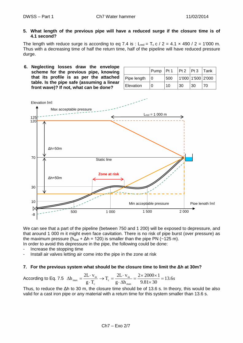
DWSS ndash Part 1 Ch7 Water hammer 11022014
Ch7 ndash Exo 27
5 What length of the previous pipe will have a reduced surge if the closure time is of 41 second
The length with reduce surge is according to eq 74 is Lred = Tc c 2 = 41 times 490 2 = 1000 m Thus with a decreasing time of half the return time half of the pipeline will have reduced pressure durge
6 Neglecting losses draw the envelope scheme for the previous pipe knowing that its profile is as per the attached table Is the pipe safe (assuming a linear front wave) If not what can be done
Pump Pt 1 Pt 2 Pt 3 Tank
Pipe length 0 500 1000 1500 2000
Elevation 0 10 30 30 70
We can see that a part of the pipeline (between 750 and 1 200) will be exposed to depressure and that around 1 000 m it might even face cavitation There is no risk of pipe burst (over pressure) as the maximum pressure (hstat + Δh = 120) is smaller than the pipe PN (~125 m) In order to avoid this depressure in the pipe the following could be done - Increase the stopping time - Install air valves letting air come into the pipe in the zone at risk
7 For the previous system what should be the closure time to limit the Δh at 30m
According to Eq 75 s61330819
120002
hg
v2LT
Tg
v2Lh
max
inc
c
inmax
Thus to reduce the Δh to 30 m the closure time should be of 136 s In theory this would be also valid for a cast iron pipe or any material with a return time for this system smaller than 136 s
Δh=50m
Static line
Lred = 1 000 m
Zone at risk
Min acceptable pressure
Max acceptable pressure
Δh=50m
500 1 000 1 500 2 000
70
30
10
120 125
Pipe length [m]
Elevation [m]
-8
DWSS ndash Part 1 Ch7 Water hammer 11022014
Ch7 ndash Exo 37
Answers to intermediary exercises
8 Draw the pressure and the velocity versus the time (Lc) at the middle of the pipe for an instantaneous valve closure taking into consideration head losses
The surge will arrive at the middle of the pipe after half of the time needed to travel the pipe L2c and come back after two times this time 2L2c=Lc
9 What are the velocity (c) the head surge (Δh) and the return time (Tr) of the pressure wave in a cast iron pipe DN200 (e=64 mm Kpipe=140 GPa) of 3 km if a pump of 170 m3h instantaneously stops working with a temperature of water of 45deg
We calculate c with Eq 7-1
pipe
water
water
K
K
e
D1
ρKc
where at 45deg Kwater is 229 GPa and ρ=9902 kgm3
The thickness e is 64 mm KCI is 140 GPa
The diameter D can be estimated as the nominal diameter (DN) so 200 mm
so ms 1237
10140
10229
64
2001
990210229
K
K
e
D1
ρKc
9
9
9
pipe
water
water
Given that the flow is totally stopped
ms 150
102004
π
1703600
A
QvΔv
23
The head surge is found with equation 7-1 Δh = Δvmiddotcg=15 times 1237 981 = 1896 m
The return time is found with equation 7-3 Tr= 2Lc= 2 times 3000 1237 = 485 s
If we compare these results with the exercise 2 we can see that they are very close the difference of taking in to consideration the water temperature of 45deg make a difference of 15 on the head surge and of 1 on the return time
pre
ssure
time
L2c
-ΔP
P0
t0 Lc 2Lc 3Lc 4Lc
+Δ
P
1 2
5Lc
3 4 Phases
t0
Reversed flow
Ve
locity
v0
Lc Lc
time Lc 2Lc 3Lc 4Lc 5Lc
DWSS ndash Part 1 Ch7 Water hammer 11022014
Ch7 ndash Exo 47
10 For the previous pipe we want to limit the head surge at 100m by having a longer stopping time what should be in this case TC
According to equation 7-5 we have s 179100819
5130002
hg
v2LT
max
inc
BY increasing significantly the closure time we will have almost half of the flow when the head surge is coming back therefore the Δv is divided by two dividing thus also the head surge by two
11 What are the velocity (c) the head surge (Δh) and the return time (Tr) of the pressure wave in a PE80 pipe PN125 OD200 (KPE=07 GPa e=182mm) of 5 km if a pump of 150 m3h instantaneously stops working with a temperature of water of 20deg
We calculate c with Eq 7-1
pipe
water
water
K
K
e
D1
ρKc
where at 20deg Kwater is 22 GPa and ρ=9982 kgm3
The nominal thickness for this pipe is given 182 mm (an average of 192 could be used)
The bulk modulus KPE is given as 07 GPa
The internal diameter D is thus per Annexe B 1636 mm
so ms 742
1070
1022
182
16361
99821022
K
K
e
D1
ρKc
9
9
9
pipe
water
water
Given that the flow is totally stopped
ms 1982
102004
π
1503600
A
QvΔv
23
The head surge is found with equation 7-1 Δh = Δvmiddotcg=1982 times 274 981 = 555 m
The return time is found with equation 7-3 Tr= 2Lc= 2 times 5000 274 = 364 s
This time if we compare these results with the exercise 3 we can see that they are not so close as the bulk modulus given is quite different from the one used in the table in annexe N
12 What are the friction coefficient (KLP) and the head losses (hLP) of the previous pipe with a roughness of 007 mm neglecting the punctual losses What is the attenuation of the negative head surge due to the losses at the tank
With equation 4-9 we find Re = D middot v ν = 1636 times 1982 101 times 10-6 = 322 000
With equation 4-19 or fig 4-5 we find λ = 00147
As the singular losses are neglected we find with equations 4-15
KLP = λ middot L D = 00147 times 5 000 01636 = 449
hLP = v2 middot λ 2g = 19822 times 449 (2 times 981) = 899 m
Thus the attenuation of the negative head surge at the tank is equal to hlosses2 about 45m In this situation where the losses are quite high as the velocity is important we can see that the remaining negative head surge at the tank is only of 10m thus the importance to take them in to account
DWSS ndash Part 1 Ch7 Water hammer 11022014
Ch7 ndash Exo 57
13 What are the attenuation of head surge at the valve (hv-att) the remaining velocity at the tank (vt1) and the attenuation of the positive head surge at the tank (ht-att) of the previous pipe
With equation 7-6 we find m 8254499812
7421-274
982144921
2gk
c1-c
vk21
h
2
2
LP
2
2
inLP
att-v
With equation 4-9 we find
m 52494981
7421-274
6071982149412
gk
c1-c
vvk12
h
ms 60712744
9821449
4c
vkv
2
2
LP
2
2
t1inLP
att-t
22
inLPt1
Thus when the surge arrive to the tank the velocity in the depression zone reaches 1607 ms This explains why the negative head surge is so small at the tanks as the difference of velocity is then only of 1982-1602=0375 ms
The attenuation of the positive head surge at the valve is of 258 m thus the positive head surge at the valve is of 555 - 258 asymp 30 m NB this value as to be added at the static level not at the dynamic one This value is much smaller than the initial head losses (899 m) thus the positive head surge is not affecting the pipe at the valve
The attenuation of the positive head surge at the tank is of 25 m thus the positive head surge at the tank is of 555 ndash 899 2 ndash 25 asymp 8 m This remaining positive head surge at the tank is very small
See the next exercise correction for an illustration of these results
14 For the previous pipe draw the developed profile of the pipeline the static and dynamic lines and the envelope schemes knowing that its profile is as per the attached table Is the pipe safe If not what can be done
Pump Pt 1 Pt 2 Pt 3 Tank
Pipe length 0 1000 1000 1000 2000
Elevation 0 0 5 10 30
As explain in the section 76 the developed profile should be used but as the slopes are small it doesnt make a big difference if it is taken into consideration or not
All the values calculated in the previous exercises were reported in this chart
It can be seen that the superior envelope is much lower than the maximum acceptable pressure thus there is no risk of pipe burst in case of water hammer
However the inferior level is lower than the ground level even lower than the cavitation line (minimum acceptable pressure) thus depressure and cavitation will happen in this pipeline if it is not protected
Possible solutions might include a pump bypass system or air valve Nevertheless into this situation the best would be to increase the diameter of the pipe decreasing also the losses and necessary PN for the pipe this will thus decrease the thickness and further the head surge
DWSS ndash Part 1 Ch7 Water hammer 11022014
Ch7 ndash Exo 67
15 What would be the effect on the head surge on the previous exercises of having a Youngs modulus (KPE)of 11 GPa instead of 07 GPa
The surge velocity will be at 341 ms instead of 274 ms increasing the head surge at 70 m instead of 56 m This will significantly increase the problematic of the depressure at the valve even for bigger diameters This shows the importance to have a good information from the supplier about the properties of the pipes and in case of doubt to take a good margin between the envelope and the maximum or minimum tolerable pressure
16 For exercise 2-4 what would be the change in ID (DN for metallic pipe) following the change in pressure due to water hammer
In order to calculate ΔD we use a formula from chapter 1 (Eq 1-5)
2e
D
K
ΔPDΔD
K is the Youngs modulus of the pipe material For the first exercise to find ΔD in mm we have
0026mm642
200
10125
1053400200ΔD
9
Therefore when the pipe will be in overpressure the DN will be Do=200+0026=200026 mm (the pipe will be expanded)
When the pipe will be in under pressure the DN will be Du= 200-0026=19997
Answers to advanced exercises
11m
Developed profile of the pipeline
-30
-10
10
30
50
70
90
110
130
0 500 1000 1500 2000 2500 3000 3500 4000 4500 5000
Dynamic or piezo line
Static line
Overpressure envelope
Depressure envelope
Pipeline
Min acceptable pressure
Max acceptable pressure
0
Elevation
PN
of
the p
ie ~
123m
Head losses
~90m
Attenuated positive head surge at the
valve ~30m
Tank elevation
~30m
Depressure ~56m
Pipe length [m]
Cavitation ~9m Head losses2
~45m
Attenuation of head surge at the valve
~26m Head losses2 +
ht-att ~48m
8m
DWSS ndash Part 1 Ch7 Water hammer 11022014
Ch7 ndash Exo 77
The same procedure is done for exercise 3 amp 4 The results are shown it the following table
Ex ΔP Pa DN or ID mm e mm K GPa ΔD mm Do mm Du mm
2
3
4
We can draw the following conclusion
even if the ΔP is bigger for cast iron the change in diameter will be less than for PE (because PE is easily distorted)
even if the ΔP is bigger for exercise 4 than for 3 the change in pipes diameter will be bigger for 3 because the wall thickness is smaller (which makes the pipe more easily distorted)
It can be noticed that the expansion due to changes in pressure in the pipe is not significant because even for PE pipe with a bigger expansion it is around half a millimetre added to the outside diameter which is less than the tolerance margin for PE pipe For example for a PE pipe having an OD of 200 mm the maximum outside diameter will be of 2012 mm (which is bigger than 2005 obtained with pressure expansion) These calculations were done for expansion due to pressure changes only because of water hammer (thus ignoring the initial pressure in the pipe) This means that the diameter can be more expanded because the total change in pressure will be bigger Furthermore if we have an initial pressure it must be checked that the PN of the pipe can bear the total pressure (initial pressure +ΔP)
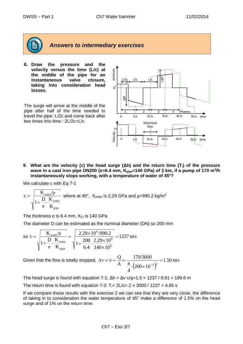
DWSS ndash Part 1 Ch7 Water hammer 11022014
Ch7 ndash Exo 77
The same procedure is done for exercise 3 amp 4 The results are shown it the following table
Ex ΔP Pa DN or ID mm e mm K GPa ΔD mm Do mm Du mm
2
3
4
We can draw the following conclusion
even if the ΔP is bigger for cast iron the change in diameter will be less than for PE (because PE is easily distorted)
even if the ΔP is bigger for exercise 4 than for 3 the change in pipes diameter will be bigger for 3 because the wall thickness is smaller (which makes the pipe more easily distorted)
It can be noticed that the expansion due to changes in pressure in the pipe is not significant because even for PE pipe with a bigger expansion it is around half a millimetre added to the outside diameter which is less than the tolerance margin for PE pipe For example for a PE pipe having an OD of 200 mm the maximum outside diameter will be of 2012 mm (which is bigger than 2005 obtained with pressure expansion) These calculations were done for expansion due to pressure changes only because of water hammer (thus ignoring the initial pressure in the pipe) This means that the diameter can be more expanded because the total change in pressure will be bigger Furthermore if we have an initial pressure it must be checked that the PN of the pipe can bear the total pressure (initial pressure +ΔP)


![ANSWERS TO ODD-NUMBERED EXERCISES M207 - Ougouagougouag.com/AnsOdds-M207.pdf · 2017-11-27 · Answers to Odd-Numbered Exercises 47. APPENDIX I ANSWERS TO EXERCISES 37. [o, 4] A63](https://img.dokumen.tips/doc/110x75/5ea264aa5c19072f7a5c9a88/answers-to-odd-numbered-exercises-m207-2017-11-27-answers-to-odd-numbered-exercises.jpg)