Theoretical

ELSEVIEi Theoretical Computer Science 171 (1997) 147-177

Computer Science

Answering queries from context-sensitive probabilistic knowledge bases’

Liem Ngo, Peter Haddawy *

lkision Systems and Artijicial Intelligence Laboratory, Department cfl Electricul Enginreriny and Computer Science, University qf Wisconsin-Mil~~aukre. Milwaukee, WI 53201. USA

Abstract

We define a language for representing context-sensitive probabilistic knowledge. A knowledge base consists of a set of universally quantified probability sentences that include context con- straints, which allow inference to be focused on only the relevant portions of the probabilistic knowledge. We provide a declarative semantics for our language. We present a query answering procedure that takes a query Q and a set of evidence E and constructs a Bayesian network to compute P(QlE). The posterior probability is then computed using any of a number of Bayesian network inference algorithms. We use the declarative semantics to prove the query procedure sound and complete. We use concepts from logic programming to justify our approach.

Keyit’ords: Reasoning under uncertainty; Bayesian networks; Probability model construction; Logic programming

1. Introduction

Bayesian networks [23] have become the most popular method for representing

and reasoning with probabilistic information [14]. But the complexity of inference

in Bayesian networks [5] limits the size of the models that can be effectively rea-

soned over. Recently, the approach known as knowledge-based model construction

[29] has attempted to address this limitation by representing probabilistic informa-

tion in a knowledge base using schematic variables and indexing schemes and then

constructing a network model tailored to each specific problem. The constructed net-

work is a subset of the domain model represented by the collection of sentences in

the knowledge base. Approaches to achieving this functionality have either focused

on practical representations and model construction algorithms, neglecting formal as-

pects of the problem [ 11,4], or they have focused on formal aspects of the knowl-

* Corresponding author. E-mail: {liem, haddawy}@cs.uwm.edu.

’ This work was partially supported by NSF grants IRI-9207262, IRI-9509165: and a Graduate School

Fellowship from the University of Wisconsin-Milwaukee.

0304.3975197/$17.00 @ 1997 -Elsevier Science B.V. All rights reserved PIf SO304-3975(96)0012X-4

148 L. Ngo, P. Haddawyl Theoretical Computer Science 171 (1997) 147-177

edge base representation language, with less concern for ease of use of the repre-

sentation and practical algorithms for constructing networks [24,2]. Hence, none of

this work has provided a practical network construction algorithm which is proven

correct.

We take a more encompassing approach to the problem by presenting a natural rep-

resentation language with a rigorous semantics together with a network construction

algorithm. In previous work [12] we started to address this problem by presenting

a framework for constructing Bayesian networks from knowledge bases of first-order

probability logic sentences. But the language used in that work was too constrained to

be applicable to many practical problems. The current paper makes three main contri-

butions. First, we define a logical language that allows probabilistic information to be

represented in a natural way and permits the probabilistic information to be qualified

by context information, when available. A knowledge base consists of a set of uni-

versally quantified sentences of the form (P(consequent 1 antecedent) = a) + context.

Second, we provide a declarative semantics for the language. Third, we present a sound

and complete query answering procedure that uses a form of SLD resolution to con-

struct Bayesian networks and then uses the networks to compute posterior probabilities.

Throughout our development we highlight the relationship between our framework and

both logic programming and Bayesian networks.

When reasoning with a large knowledge base, context information is necessary in

order to focus attention on only the relevant portions. Consider the following moti-

vating example, which will be referred to throughout the remainder of the paper. A

burglary alarm could be triggered by a burglary, an earthquake, or a tornado. The

likelihood of a burglary is influenced by the type of neighborhood one resides in. In

different contexts, people might have different beliefs concerning the probabilistic re-

lations between these variables. Someone who resides in California might think of an

earthquake when he hears an alarm. If he lived in Wisconsin instead, he might relate

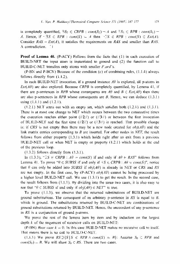
that event with a possible tornado. Two networks representing these two different con-

texts are shown in Fig. 1. Many problems, like this one, will naturally contain some

deterministic information that can be used as context to index relevant probabilistic

relations. For simplicity of exposition, we have chosen this toy problem to use as a

running example to illustrative the details of the formalism. A discussion of some prac-

tical problems in which such deterministic information can be identified is provided in

Section 6.

2. Representation language

Throughout this paper, we use P and sometimes P * to denote a probability distri-

bution; A,B,. . . with possible subscripts to denote atoms; names starting with a cap-

ital letter or X to denote domain variables; and p,q,. . . with possible subscripts to

denote predicates. We distinguish two types of predicates: context and probabilistic

predicates.

L Nqo. P. Haddmyl Theoretical Computer Science 171 (1997) 147- 177 119

live_in(X. cdifomla)

(b)

Fig. I. An example of context-dependent bellef’s.

Context predicates (c-predicates) have value true or false and are deterministic. They

are used to describe the context the agent is in and to eliminate unnecessary or inappro-

priate probabilistic information from consideration by the agent. An atom formed from

a context predicate is called a context atom (c-atom). A context literal (c-literal) is

either a c-atom or the negation of a c-atom. A context base is a normal logic program

[ 171, which is a set of universally quantified sentences of the form Co + L 1, L2,. . L,,.

where n is a nonnegative integer, c stands for implication, comma for logical conjunc-

tion, Co for a c-atom, and Li, 1 <i<n, for c-literals. We use completed logic programs

proposed by Clark [17] for the semantics of the context base. Essentially, a completed

logic program is formed from a logic program by adding to it (1) some clauses so that

the clauses in the original program become the only definitions of the predicates in

the program, and (2) the equality theory to interpret the introduced equality predicate

[171. Each probabilistic predicate (p-predicate) represents a class of similar random vari-

ables. P-predicates appear in probabilistic sentences and are the focus of probabilistic

inference processes. An atom formed from a p-predicate is called a probabilistic atom

(p-atom). Queries and evidence are expressed as p-atoms. In the probability models we

consider, each random variable can assume a value from a finite set and in each possible

realization of the world, that variable can have one and only one value. We capture this

property by requiring that each p-predicate have at least one attribute, which represents

the value of the corresponding random variable. For predicates with multiple attributes,

the value attribute is always the last. For example, the random variable neighborhood of

a person x can have value bad, average, good and can be represented by a two-position

predicate - the first position indicates the person and the second indicates the type of

that person’s neighborhood. A p-predicate with multiple attributes represents a set of

related random variables - one for each ground instance of the non-value attributes. As-

sociated with each p-predicate p must be a statement of the form vAL( p) = { ~‘1.. , L.,, }.

where cl,. , u, are constants denoting the possible values of the corresponding random

variables.

150 L. Ngo, P. Haddawyl Theoretical Computer Science 171 (1997) 147-177

Definition 1. Let A = p(tl , . . , &_I, t,,,) be a p-atom, we use obj(A) to designate the

tuple (P,ti,..., t,_l ) and uaZ(A) to designate tm. If A is a p-atom of predicate p, then

VAL(A) means ML(p). If A is a ground p-atom then obj(A) represents a concrete

random variable in the model and vaZ(A) is its value. We also define Ext(A), the

extension ofA, to be the set {p(tl,...,t,_l,vi)I l<i<n}.

If A is a ground p-atom, we assume that the elements of &t(A) are mutually ex-

clusive and exhaustive: in each “possible world”, one and only one element in _&t(A)

is true. We assume that the attributes of p-predicates are typed, so that each attribute

is assigned values in some well-defined domain.

Example 2. In the context of our running example, the declarations nbrhd(Somebody :

Person, V) and VAL(nbrhd) = {bad, average, good} say that the first attribute of nbrhd

is a value in the domain Person, which is the set of all persons, and the second

attribute can take values in the set {bud, average, good}. For a person, say named

John, nbrhd( john, good) means that the random variable “neighborhood of John”, in-

dicated in the language by obj(nbrhd(john,good)), is “good”, indicated in the lan-

guage by val(nbrhd( john, good)) = good. In any possible world, one and only one of

the following atoms is true: nbrhd( john, bad), nbrhd( john, average), and nbrhd( john,

good).

We denote the set of all such predicate declarations in a knowledge base by PD.

A probabilistic sentence (p-sentence) has the form (P(AolAl,.. .,A,) = a) +

Ll,..., L, where n 30, m 3 0, 0 < c( < 1, Aj are p-atoms, and Lj are c-literals. The

sentence can have free variables and each free variable is universally quantified over

the entire scope of the sentence. The above sentence is called context-free if m =

0. If S is the above probabilistic sentence, we define context(S) to be the conjunc-

tion L1 A ... A L,, prob(S) to be the probabilistic statement P(AolAl,. . . ,A,) = CC,

ante(S) to be the conjunction Al A . . . A A,,, and cons(S) to be Ao. For convenience,

sometimes we take ante(S) to be the set of the conjuncts. We call A0 the conse-

quent of 5’. A probabilistic base (PB) of a knowledge base is a finite set of p-

sentences.

Definition 3. Let A be a (p- or c-) atom. We define ground(A) to be the set of all

ground instances of A satisfying the domain (type) constraints. If E is a set of p-atoms

then ground(E) = U {g round(A) 1 A E E}. Let S be a p-sentence. We define ground(S)

to be the set of all ground instances of S satisfying the domain constraints.

A set of ground p-atoms {Ai 1 1 <i <n} is called coherent if V’i, j (1 <i,j <n) :

obj(Ai) = obj(Aj) + UaZ(Ai) = Cal.

A PB will typically not be a complete specification of a probability distribution over

the random variables represented by the p-atoms, One type of information that may

be lacking is the specification of the probability of a variable given combinations of

I_. Ngo, P. Haddawyl Theoretical Computer Science 171 11997) 147-177 151

values of two or more variables that influence it. For real-world applications, this type

of information can be difficult to obtain. For example, for two diseases Dt and 02 and

a symptom S we may know P(SIDt ) and P(SI&) but not P(SID,,D>). Combining

rules such as generalized noisy-OR [6,26] are commonly used to construct such com-

bined influences.

We define a combining rule as any algorithm that

(i) takes as input a set of ground p-sentences that have the same consequent

{Pv(AoslA,i,. , A,, ) = Xi 1 1 <i <m} where nz is a non-negative integer or infinity,

and

(ii) produces as output a set of ground p-sentences OS = {Pr(AolBil,. , B,k, ) =

PI 1 I <i <h, h and k, are some non-negative finite integers} such that

(a) the antecedent of each p-sentence in OS is a coherent set,

(b) if Sl and S2 are two different p-sentences in OS then unte(S1) U ante(&) is not

coherent, and

(c) if B appears in the antecedent of a p-sentence in OS then &j(B) E

UT”=, {obj(A,i ), , obj(&, I}; and (iii) the output set is empty if and only if the input set is empty.

Condition (b) enforces the constraint that at most one antecedent is true in any

possible world. As a result, in each possible world there is at most one statement

about the direct influences on the consequent A 0. Condition (c) is natural: we do not

want to introduce new random variables.

We assume that for each p-predicate p, there exists a corresponding combining rule

in CR, the combining rules component of the KB. Each combining rule is applied

only once for any given predicate. The combining rules are specified by the designer

of a knowledge base and they reflect his conception of the interaction between direct

influences of the same random variable.

A knowledge base (KB) consists of predicate descriptions, a probabilistic base, a

context base, and a set of combining rules. We write KB = (PD, PB, CB, CR).

Fig. 2 shows a possible knowledge base for representing the burglary example in-

troduced in the previous section. We have the following p-predicates: nhrhd, burgfury,

quake, ularm, and tornado. In Example 2 we gave the interpretation of the statements

nbrhd(Somehody : Person, V) and VAL(nbrhd) = {bud, uceruge, good}. Similar inter-

pretations apply to other statements in PD.

PB contains the p-sentences. Due to space limitations, we cannot show all the sen-

tences. We would have sentences describing the conditional probabilities that the ran-

dom variables corresponding to burglary and alarm achieve the value no, and the

marginal probability for quake achieving the value no. CB specifies relationships in the

context information. For example, the first two clauses, define the predicate live-in: if

a person X lives in the area Y then she lives in Y; if she lives in Y and Y is in Z

then she also lives in Z. The last clause in CB declares that Madison is in Wisconsin.

Most of the probabilistic sentences in PB are annotated by the corresponding context.

For example, if a person lives in California then the chance that her neighborhood is

bad is 0.3. The 7 operator is negation-as-failure used in logic programming to encode

152

PD ={

PB ={

(Sl)

(‘92)

(S3)

(54)

(S5)

(s6)

(S7)

(‘%)

(S9)

(SlO)

(Sll)

(Sl2)

(Sl3)

(514)

(‘%5)

ts16)

(Sl7)

(‘%a)

(Sl9)

(‘720)

L. Ngo, P. Haddawyl Theoretical Computer Science 171 (1997) 147-177

nbrhd(Somebody : Person, V), VAL(nbrhd) = {bad, average,good};

burglary(Somebody : Person, V), VAL(burglary) = {yes, no};

quake(SomeaTea : Area, V), VAL(quake) = {yes, no};

alarm(Somebody : Person, V), VAL(alarm) = {yes, no};

tornado(Sonearea : Area, V), VAL(tornado) = {yes, no}}

P(nbrhd(X, average)) = .4

P(nbThd(X, bad)) = .3 c live_in(X,california)

P(nbrhd(X,good)) = .3 c live_in(X, california)

P(nbrhd(X, bad)) = .2 + live_in(X,wisconsin)

P(nbrhd(X,good)) = .4 + livein(X, wisconsin)

P(buTgkzry(X, yes)lnbrhd(X, average)) = .4

P(burglary(X,yes)lnb7hd(X,good)) = .3 + [ive_in(X,california)

P(burgla~y(X,yes)Jnb~hd(X, bad)) = .6 + live_in(X, cafifornia)

P(burglary(X, yes))nbrhd(X, good)) = .2 + live-in(X,wisconsin), burglarized(X)

P(burglary(X,yes)Jnbrhd(X, bad)) = .4 + live&(X, wisconsin), burglarized(X)

P(burgIary(X,yes)(nbrhd(X, good)) = .I5 + live-&(X, wisconsin), -burglarized(X)

P(bwglary(X,yes)lnbrhd(X, bad)) = .3 + livein(X,wisconsin), -burglarized(X)

P(alawn(X,yes)Jtornado(Y, yes)) = .99 + livein(X, wisconsin), in_area(X, Y)

P(alawn(X,yes)Jtornado(Y,no)) = .l + Iive_in(X,wisconsin), in_area(X, Y)

P(aZa+m(X,yes)[bwglasy(X, yes)) = .98

P(alarn(X,yes)(burglary(X,no)) = .05

P(alarm(X,yes)Iquake(Y, yes)) = .99 + live_in(X,california),in_area(X,Y)

P(alarm(X,yes)Iquake(Y, no)) = .15 + live&(X, California), in_area(X,Y)

P(quake(Y, yes)) = .2 + in(Y, California)

P(tornado(Y,yes)) = .l + in(Y, zuisconsin)

($1) P(tornado(Y,no)) = .9 + in(Y,zuisconsin)

.I. )

CB = { l;vein(X, Z) + live_in(X,Y),in(Y, Z)

live-+X, Y) + in_area(X,Y)

in(madison, u&con&)}

CR = { Generalized-Noisy-OR}

Fig. 2. Example knowledge base.

nonmonotonic reasoning. Finally, Generalized Noisy-OR is used as the combining rule

for all p-predicates.

We can see that a KB has a two-layer structure. The lower layer is the normal pro-

gram CB whose semantics is used to select the relevant p-sentences from the upper

layer PB. That selection process, which is presented in the following sections, is per-

formed dynamically for each given set of context information and set of evidence.

L. Ngo, P. Haddmy I Theoretical (hmputer Scium 171 i 1997) 147- I77 153

3. Declarative semantics

In this section we give a declarative characterization of the probabilistic information

implied by a KB in a concrete context with a given set of evidence. The concepts here

are defined without reference to any particular query-answering procedure. Following

the currently common way of characterizing the semantics of a logic program [9,8], we

define the relevant set of atoms in a bottom-up manner from antecedent to consequent.

In contrast, the query-answering procedure presented in Section 4 functions in a top-

down manner.

3. I. The relevant knowledge base

It can be difficult for a user to guarantee global consistency of a large probabilisitic

knowledge base, especially when we allow context-dependent specifications. We define

our semantics so that we need consider only that portion of a knowledge base relevant

to a given problem. Thus, if part of the knowledge base is inconsistent, this will not

affect reasoning in all contexts.

Definition 4. A set of ecidence E is simply a set of p-atoms such that ground(E) is

coherent. A set of context information C is any set of c-atoms.

In a particular inference session, characterized by a set of context information and a

set of evidence, only a portion of the KB will be relevant. The set of relevant atoms is

the set of evidence, the set of atoms whose marginal probability is directly stated, and

the set of atoms influenced by these two sets, as indexed by the context information.

In constructing the set of relevant p-atoms, we consider only the qualitative depen-

dencies described by probabilistic sentences. If (P(AoI.41, ,A,) = c() t LI, .L,,

is a ground instance of a sentence in PB conforming to domain type constraints and

LI A A L,, can be deduced from completed(C U CB), then that sentence indicates

that Aa is directly influenced (or caused) by Al,. . ,A,, in the current context. If, in

addition, A 1.. , A,l are relevant p-atoms then it is natural to consider A0 as relevant.

Let c,ompleted(C U CB) be the completed logic program with the associated r+~llir_i~

theory [ 171 constructed from C U CB, then we have the following definition of the set

of relevant p-atoms,

Definition 5. Assume a set of evidence E, a set of context information C, and a KB.

The set of relevant p-atoms (RAS) is defined as the smallest set R statisfying the

following conditions:

(i) ground(E) G R;

(ii) if S is a ground instance of a p-sentence in PB, conforming to domain con-

straints, such that context(S) is a logical consequence of completed(C U CB) and

ante(S) i R then cons(S) E R;

(iii) if a p-atom A is in R then Ext(A) C R.

154 L. Nyo. P. Haddawyl Theoretical Computer Science 171 (1997) 147-177

The MS is constructed in a way similar to Herbrand least models for Horn programs.

Context information is used to eliminate that portion of PB not related to the current

problem.

Definition 6. Let E be a set of evidence. We define the set of p-sentences describing

the evidence E, denoted by EBase, as U {AQround(E)l(P(4 = 1) u {PM) = 0 IA’ E Ext(A) A A’ # A}).

The relationship between our KBs and logic programs is demonstrated in the fol-

lowing definition and property.

Definition 7. Given a set of evidence E, a set of context information C, and a KB;

the Horn version of (E, C, KB), denoted by Horn(E, C, KB), is a Horn logic program

defined in the following way:

(i) Let RI be the set of all prob(S), where S is a ground instance of some

p-sentence in PB, conforming to domain constraints, such that context(S) is a logi-

cal consequence of completed(C U CB).

(ii) Let S be the p-sentence P(AoIAl, . , A,) = CI. We define clause(S) to be the set

of all Horn clauses B0 c A 1,. . ,A,, where Bo is an arbitrary element in Ext(Ao).

Then Horn(E, C, KB) = (UfSER, I clause(S)) U ({Ext(A) 1 A E ground(E)}).

Proposition 8. Given a set of evidence E, a set of context information C, and a KB;

RAS always exists and is equal to the least Herbrand model qf Horn(E, C,KB).

Definition 9. Given a set of evidence E, a set of context information C, and a KB; the

set of relevant p-sentences (RPB) is constructed in the following way:

(i) Let R be the set of all prob(S) such that S is a ground instance of a p-sentence

in PB, context(S) is a logical consequence of completed(C U CB), cons(S) E RAS, and

ante(S) 2 RAS.

(ii) If A E ground(E) and +lS E R : cons(S) E Ext(A) then add to R the following

set: {P(A)= ~}U{P(A’)=OIA’EE~~(A)~\A#A’}.

RPB is the final set R.

If S is a p-sentence in RPB then S originates from either (a p-sentence in) PB or

EBase. Condition (ii) augments the knowledge base KB with new knowledge about

the evidence. The following example illustrates this point.

Example 10. Let PB = {P(q(true)Jr(true))=0.7; P(q(faZse)(r(true))=0.3; P(q(true)(

r(false)) = 0.5; P(q(false)lr(faZse)) = 0.5). Without evidence, MS and RPB are both

empty. Suppose the set of evidence is E = {r(true)}. Then the corresponding RAS is

{q(true), q( false), r(true), r( false)} and RPB = PB U {P(r(true)) = 1, P(r(j&e)) =

0). Notice that RPB contains two p-sentences which are introduced by the second step

of Definition 9. These two p-sentences are necessary to build the link matrix for the

evidence r(tvue).

L. Ngo, P. Haddawyl Theoretical Computer Sc~iencr 171 (1997) 147-177 155

The RPB contains the basic influences among p-atoms in RAS. In the case of multiple

influences represented by multiple sentences, we need combining rules to construct the

combined probabilistic influence.

Definition 11. Given a set of evidence E, a set of context information C, and a KB;

the set of combined reletunt p-sentences (CRPB) is constructed by applying the cor-

responding combining rule to each maximal set of sentences {Sr, . , &} in RPB for

which the elements have the same consequent.

CRPBs are analogous to completed logic programs. We assume that each sentence

in CRPB describes all random variables that directly influence the random variable in

the consequent.

Example 12. Consider our burglary example and suppose we have the evidence E =

{ hurglury(john, yes)} and the context C’= { in_area( john, madison), hurglurized( john)}.

In this case,

IUS ={nhrhd( john, bud), nhrhd( john, cluerage), nbrhd( john, good), burglury( john,j>es ).

hurglary( john, no), alarm( john, yes), alarm( jokn, no), tornudo(mudison, yes),

totwudo(madison, no)}

RPB = {P(nhrhd( john, average)) = 0.4, P(nbrhd( john, bud)) = 0.2,

P(nhrhd( john, good)) = 0.4, P(hurglur_v( john, yes)Inhrhd(john, average)) = 0.4.

P(hurybry( john, yes)lnhrhd( john, good)) = 0.2,

P(hurylury(John, yes)lnhrhd( john, bud)) = 0.4,

P(alurm(john, yes)Itornudo(mudison, yes)) = 0.99,

P(alurm(john, yes)lburgkury(john, yes)) = 0.98,

P(u~urm(john,yes)(burgfury(john,no)) = 0.05,

P(ulurm(.john, yes)(tornudo(mudison,no)) = 0.1,

P(burglury( john, no)lnbrhd(john, good)) = 0.8,

P(hurglury( john, no)lnhrhd( john,uveruge)) = 0.6,

P(hurglury(,john, no)lnbrhd( john, bud)) = 0.6,

P(ulurm( john, no)(tornudo(mudison, yes)) = 0.01.

P (ularm(john, no)lburgfury( john, yes)) = 0.02,

P(ulurm(john,no)jhurglury(john,no)) = 0.95,

P(ulurm( john. no)\tornado(madison, no)) = 0.9, P(tornado(madison, yes)) = 0.1.

P( tornudo(mudison, no)) = 0.9).

In the CRPB the sentences in RPB with ularm(john,.) as the consequent are trans-

formed into sentences specifying the probability of alarm conditioned on both hurglur?

and tornado using a generalization of Noisy-OR:

P(alarm( john, yes)ltornado(mudison, yes), hurgfury( john, yes)) = 0.9998,

P(alurm( john, yes)ltornado(madison, yes),burglury( john, no)) = 0.98,

P(ularm(john, yes)\tornudo(mudison, no), hurglary( john, yes)) = 0.99,

P(alarm(john, yes)(tornudo(mudison, no), hurgfury( john, no)) = 0.9,

P(ulurm(john, no)(tornado(mudison, yes), burglury( john, yes)) = 0.0002,

156 L. Ngo. P. Haddawyl Theoretical Computer Science 171 (1997) 147-l 77

P(aZarm(john, no)~tornado(madi.son, Jes), burglury(john, no)) = 0.02,

P(alarm(john, no)ltornado(mudison, no), buvglary(john, yes)) = 0.01, and

P(uZarnz(john, no)ltornudo(mudison, no), burglary( john, no)) = 0.1,

The other sentences in RPB are carried over to CRPB unchanged.

We define a syntactic property of CRPB that is necessary in constructing Bayesian

networks from the KB.

Definition 13. A CRPB is completely quantzjied if

(i) for all ground atoms A0 in MS, there exists at least one sentence in CRPB with

A0 in the consequent; and

(ii) for all ground sentences S of the form P(AolAl, . . . , A,) = x in CRPB we have

the following property: For all i = 0,. . , n, if Aj is p(?, a), where ? is a list of ground

terms, and v’ is a value in VAL(p), such that v # v’, then there exists another ground

sentence S’ in CRPB such that S’ can be constructed from S by replacing Ai by p(?, v’)

and c( by some M’.

If we think of each ground obj(A), where A is some p-atom, as representing a random

variable in a Bayesian network model, then the above condition implies that we can

construct a link matrix for each random variable in the model. This is a generalization

of constraint (Cl ) in [ 121. We do not require the existence of link matrix for every

random variable, but only for the random variables that are relevant to an inference

problem.

3.2. Probabilistic independence assumption

In addition to the probabilitistic quantities given in a PB, we assume some probabilis-

tic independence relationships specified by the structure of the p-sentences. Probabilistic

independence assumptions are used in all related work [29,4, 11,24, 121 as the main

device to construct a probability distribution from local conditional probabilities. Un-

like Poole [24], who assumes independence on the set of consistent “assumable” atoms,

we formulate the independence assumption in our framework by using the structure of

the sentences in CRPB. We find this approach more natural since the structure of

the CRPB tends to reflect the causal structure of the domain and independencies are

naturally thought of causally.

Definition 14. Let R be a set of ground context-free p-sentences and let A and B be

two ground p-atoms. We say A is in&enced by B in R if

(i) there exists a sentence S E R, an atom A’ in Ext(A), and an atom B’ in Ext(B)

such that A’ = cons(S) and B’ E ante(S) or

(ii) there exists another ground p-atom C such that A is influenced by C in R and C

is influenced by B in R.

Example 15. Continuing the burglary example, ularm(john,yes) is influenced by

nbrhd(john,good), nbrhd(john, bud), burglury(john, yes), and tornado(mudison, no).

L. Nyo. P. Haddawyl Throreticwl Computer Scirnw 171 f 1997) 147 -I 77 157

Assumption. We assume that ij” P(AoIA,,. . . , A,,) = x is in CRPB then ,for all ground

p-atoms B,. , B, which are not in E_xt(Ao) and not influenced by A0 in CRPB,

A0 and BI. . B,, are probabilistically independent given Al.. ,A,,. This mtwns thut

P(AoIB,, . . . . &,,A I,..., A,) = P(Ao(A ,,..., A,).

Example 16. We have alurm(john,yes) is probabilistically independent of nhrhd

( john, good ) and nhrhd( john, bad) given burglury( john. yes) and tornado( mudiwz.

no).

3.3. Model theorll

We define the semantics by using possible worlds on the Herbrand base. This ap-

proach of characterizing the semantics by canonical Herbrand models is widely used

in work on logic programming [S, 91. In our semantics, the context constraints in the

context base CB and the set of context information C act to select the appropriate set

of the possible worlds over which to evaluate the probabilistic part of the sentences.

In this way they index probability distributions.

The RAS contains all relevant atoms for an inference session. We assume that in

such a concrete situation, the belief of an agent can be formulated in terms of possible

tnodels on RAS.

Definition 17. Assume a set of evidence E, a set of context information C. and a KB.

A possible model M of the corresponding CRPB is a set of ground atoms in RAS

such that for all A in IS’S, k%(A) n M has one and only one element. The atoms

in M represent the set of atoms assigned the value true; all other atoms are assigned

the value false.

A probability distribution on the possible models is realized by probability density

assignment to each model. Let P be a probability distribution on the possible models.

we define P(Al,. . , A,I), where AI,. . . , A, are atoms in RAS, as C {P(w)lw is a possible

model containing Ai,. . ,A,}. We take a sentence of the form P(AoIA,, ,A,,) = CI. as

shorthand for P(Ao,A 1,. . , A,) = x x P(A,, . , A, ), so that probabilities conditioned

on zero are not problematic. We say P satisfies a sentence P(AoIA,, . A,, ) = T if

P(Ao, Al,. . . A,,) = x x P(A1,. , A,) and P satisfies CRPB if it satisfies every sentence

in CRPB.

Definition 18. A probability distribution induced by the set of evidence E, the set of

context information C, and KB is a probability distribution on possible models of C’RPB

satisfying CRPB and the independence assumptions implied by CRPB.

Example 19. If a CRPB is incompletely quantified, many possible distributions may

satisfy it. For example, if CRPB = {P(nbrhd(john, bud)) = 0.5, P(tornado(lrzatfi,ison,

yzs)) = 0.6, P(tornado(madison,no)) = 0.4) and nbrhd can take one of the three val-

ues bad.aceruge, good, then any probability assignment P* such that P*(nhrhd( john,

158 L. Ngo, P. HaddawyI Theoretical Computer Science 171 (1997) 147-177

bad)) = 0.5 and P*(rzbrhd(john,averuge)) + ~*(nbrhd(john,good)) = 0.5 is an in-

duced probability distribution.

We define the consistency property only on the relevant part of a KB. Since the

entire KB contains information about various contexts, testing for consistency of such

a KB may be very difficult.

Definition 20. A completely quantified CRPB is consistent if

(i) there is no atom in RAS which is influenced by itself;

(ii) if P(Ao(Al , . . ,A,) = c( is in CRPB then P(AolAl,. . ,A,) = 2’ is not in CRPB,

for any a’ # a; and

(iii) for all P(AolA,, . . . ,A,) = c( in CRPB, C {rjlP(Ab(A~, . . ,A,) = sli E CRPB and

obj(&) = obj(&)} = 1.

Condition (i) rules out cycles and condition (iii) enforces the usual constraint that

the probabilities of the values of a random variable sum to one. The following example

shows that PB may contain cycles but a specific completely quantified CRPB is still

consistent.

Example 21. Let PB={P(p(trz~e)Jp(true))= 1; P(p(true)lp(faZse))= 1; P(p(faZse)l p(true))= 1; P(p(faZse)(p(fuZse)) = 1; P(q(true)lr(true))=0.7;P(q(faZse)lr(true))= 0.3; P(q(true)(r(fuZse)) = 0.5; P(q(faZse)lr(faZse)) = 0.5}. PB contains a cycle (p is

influenced by itself) and the probability assignment is not reasonable (P(p(fuZse)l p(true)) = 1). Assume the set of evidence is E = {r(true)}. The CRPB {P(q(true)J

r(true)) = 0.7; P(q(fuZse)lr(true)) = 0.3; P(q(true)lr(fuZse)) = 0.5; P(q(fuZse)l r(fuZse)) = 0.5; P(r(true)) = 1; P(r(fuZse)) = 0} IS completely quantified and con-

sistent. Notice that the presence of the evidence E causes the information about q and

Y to be taken into account and since p is not in RAS, the information about it is

discarded.

Theorem 22. Assume a set of evidence E, a set of context information C, and a KB. If RAS is finite and the completely quantzjied CRPB is consistent, then there exists one and on& one induced probability distribution.

3.4. Probabilistic queries

In one inference session, we can pose queries to ask for the posterior probabilities

of some random variables.

Definition 23. A complete ground query w.r.t. the set of evidence E and the set of

context information C is a query of the form P(Q) =?, where the last attribute of Q

is a variable and it is the only variable in Q. The meaning of such a query is: find the

posterior probability distribution of obj(Q). If ML(Q) = {VI,. . , u,} then the answer

to such a query is a vector (~1,. . , cx,), where aci is the posterior probability that obj(Q) receives the value vi.

L. Nyo, P. Huddawyl Theoretical Computer S&rzcc 171 f 1997) 147-177 IS9

A complete query is a query of the form P(Q) = ?, where the last attribute of Q is

a variable and the other attributes may also contain variables.

Example 24. We can pose the following complete ground query to the example KB:

P(ulavm(,john, V)) = ‘? to ask for the posterior probability of John’s alarm status.

Definition 25. Assume a set of evidence E, a set of context information C, a KB. and

a complete ground query P(Q) =?, where V&(Q) = (~‘1,. . . cn}. We say P(Q) =

(XI,. . , r, ) is a logical corzsequener of (E, C, I(B) if for all probability distributions P*

induced by E. C, and KB, ‘di (OGidn) : P*({MIQl and ground(E) are true in A4 } ) =

x, x P*({Mlgr-ound(E) are true in M}), where Qi is Q after replacing val(Q) by I‘,.

Example 26. Continuing Example 19, suppose we have the query P(torrwdo

(madison. V)) =?. There are an infinite number of induced probability distributions

but in all of them P(tornudo(madison,_yes)) = 0.6 and P(tornado(n~udison,no)) = 0.4.

So the two sentences are logical consequences of CRPB.

In order to prove that the answers returned by our query answering procedure are

correct, we must precisely define the notion of a correct answer to a query.

Definition 27. Assume a set of evidence E, a set of context information C. a KB, and

a complete ground query P(Q) = ?. Then P(Q) = ( al,. . . x,) is a correct unsww to

the complete ground query P(Q) =? if P(Q) = (xl,. . , a,) is a logical consequence

of (E, C, KB)

If P(Q) = ? is a complete query then P(Q’) = (a~, . . , x,, ) is a correcf ans~~vr to the

complete query P(Q) = ? if Q’ is formed from a ground instance of Q by substituting

its last attribute by a new variable name and P(Q’) = (xi,. , r,) is a correct answer

to the complete ground query P(Q’) = ?.

Definition 28. Assume a set of evidence E, a set of context information C, and a KB

are given. We say a query answering procedure is sound (w.r.t. complete queries) if

for any complete query P(Q) =?, any answer returned by the procedure is correct.

We say a query answering procedure is complete (w.r.t. complete queries) if for any

complete query P(Q) = ?, any correct answer is returned by the procedure after a finite

amount of time.

4. Query answering procedure

Our query answering procedure has the following steps: build the necessary portion

of the Bayesian network, each node of which corresponds to an obj(A), where A is

a ground p-atom in RAS; update the Bayesian network using the set of evidence E;

and output the updated belief of the query nodes. The main idea of the algorithm is

to build a supporting network for each random variable corresponding to a ground

instance of an evidence atom or the query.

160 L. Ngo, P. Haddawyl Theoretical Conzpuler Science 171 (1997) 147-177

4.1. Supporting networks

Definition 29. Let X be a node in a Bayesian network JV. The supporting network

~2’ of X in JV” is the smallest subnetwork of JV such that

(i) X is in _4#.

(ii) For any node Y in -4, every parent of Y is in ~2’.

(iii) Any link (or link matrix) in .M that relates only to nodes in J? is in &‘.

Let XI,. . . ,X, be nodes in JV. The supporting network of XI,. . ,X, is the union of

the supporting networks for each Xi, 1 <i <n..

Example 30. The supporting network of the random variable burglary in each network

shown in Fig. 1 consists of two nodes (burglary and neighborhood), the link between

them, and the corresponding link matrices.

Building a supporting network instead of the whole network to answer a query is

justified by the fact that atoms that do not influence either the evidence or the query

are irrelevant.

Proposition 31. Let ./lr be a Bayesian network, X be a node in .,V, and E be the ev-

idenee that relates to nodes in ~5~. Then the posterior probability of X given the

evidence E does not depend on nodes outside the supporting network of X and

the nodes related to E.

The correspondence between a CRPB and the network it represents is shown in the

following proposition.

Proposition 32. Assume a set of evidence E, a set of context information C, and

a KB are given. If the corresponding CRPB is completely quantified and consistent

then:

(i) There exists a Bayesian network model x of the unique probability distribution

induced by CRPB.

(ii) Let A and B be two ground p-atoms in RAS. B injluences A in CRPB if and

only if the node corresponding to obj(B) is in the supporting network of the node

corresponding to obj(A) in Jlr, and the two nodes are d@erent.

Each p-sentence in CRPB corresponds to a link matrix entry in the Bayesian network.

Because of the direct correspondence between CRPB and the Bayesian network it

represents, we will sometimes refer to “the portion of CRPB supporting A (or obj(A))“,

where A is a ground p-atom, to indicate the supporting network of obj(A). Similarly,

we will refer to “the portion of CRPB supporting a set of ground p-atoms.”

4.2. Q-procedure

In this section we present an algorithm, Q-procedure, for answering complete queries

P(Q) = ?, given E, C, and k3. We assume that the domains are finite. Because of the

L. Nqo, P. Haddabvyl Theoreticul Computer Science 171 (1997) 147-177 161

similarity between RPB and the Horn logic program Horn(E, C, KB) (see Section 3. I ),

Q-procedure’s performance is similar to that of SLD resolution with the depth-first

search strategy and with the formation of lemmas during its execution. Every time all

p-sentences in RPB which have the same p-atom B as consequent have been collected,

Q-procedure stores them in a node of a partially generated Bayesian network and later

uses B as a lemma to avoid building the proof tree of B again. Q-procedure works

correctly on acyclic PBS.

Definition 33. A PB is called acyclic if there is a mapping P_ord() from the set

of ground instances of p-atoms into the set of natural numbers such that (I ) For

any ground instance (P(Ao + Al ,...,, 4,) = 2) + .LI ,..., L, of some clause in PB,

P_ord(Ao) > P_ord(A,),‘di : I <i<n. (2) For any ground p-atom A, P-o&(A) =

P_ord(A’),VA’ E ,%(A).

For example, our burglary problem has an acyclic PB. The expressiveness of acyclic

logic programs is demonstrated in [l]. We hope that acyclic PBS have equal importance.

To the best of our knowledge, PBS with cycles are considered problematic and all PBS

considered in the literature are acyclic, e.g. [24].

The pseudo-code for Q-procedure is shown in Fig. 3. The FOR loop constructs the

supporting network for the set of evidence and the final BUILD-NET call augments

the constructed network with the supporting network of ground instances of the query.

UPDATE(NET, E) is any probability propagation algorithm on Bayesian networks.

The supporting networks are constructed via calls to the BUILD-NET function.

BUILD-NET receives as input an atom, whose supporting network needs to be ex-

Q-PROCEDURE BEGIN

NET:= {};

EBase := UjaGgrOUnd(Ejl({P(A) = 1) u {P(B) = O(B E Ezt(A) A A # R}):

Extended_PB := PB u EBase; { Build the subnetwork that supports the evidence }

FOR each E; E E DO BEGIN temp := BUILD-NET(E,, NET, EztendedPB);

END:, { Build the subnetwork that supports the ground instances of the query }

SUBSS := BUILD-NET (Q, NET, EztendedYB); { Prune the isolated portions of the network }

FOR each obj(A) such that A E ground(E) DO IF there is no path connecting obj(A)

and a node corresponding to a ground instance of the query

THEN delete the supporting network of obj(A) { Perform the probability propagation on NET}

UPDATE(NET,E); { Output posterior probabilities } FOR each B in SUBSS output the probability values at node obj(QS);

END.

Fig. 3. Query processing procedure

162 L. Ngo, P. Haddawy I Theoretical Computer Science 171 (1997) 147-177

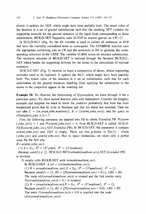
plored. It updates the NET, which might have been partially built. The return value of

the function is a set of ground substitutions such that the resulting NET contains the

supporting network for the ground instances of the input atom corresponding to those

substitutions. BUILD-NET frequently calls SLDNF to answer queries on CB U C.

In BUILD-NET (Fig. 4), the RS variable is used to collect all sentences in RPB

that have the currently considered atom as consequent. The COMBINE function uses

the appropriate combining rule in CR and the sentences in RS to generate the corre-

sponding sentences in the CRPB. The variable SUBSS stores all returned substitutions.

The recursive structure of BUILD-NET is realized through the function BUILD-C-

NET which builds the supporting network for the atoms in the antecedents of relevant

sentences.

BUILD-C-NET (Fig. 5) receives as input a conjunction of atoms, whose supporting

networks need to be explored. It updates the NET, which might have been partially

built. The return value of the function is a set of substitutions such that for each

substitution all the ground instances resulting from applying the substitution to the

atoms in the conjuction appear in the resulting net.

Example 34. To illustrate the functioning of Q-procedure, we trace through it for a

particular query. We show nested function calls with indentation. Consider the burglary

example and suppose we want to know the posterior probability that John has been

burglarized given that he lives in Madison and that his alarm has sounded. Then we

can take C = {in_area(john,madison)}, E = {alarm( john, yes)}, and the query as

P(burglary( john,X)) = ?.

First, the following sentences are inserted into PB to obtain ExtendedPB: P(alarm

(john, yes)) = 1 and P(alarm(john,no)) = 0. Next BUILD-NET is called: BUILD-

NET(alarm( john, yes), NET, Extended-PB). In BUILD-NET, the parameter A contains

alarm( john, yes) and NET is empty. There are two p-atoms in Ext(A) : alarm

(john, yes) and alarm( john,no). Due to space limitations, we show only a partial

trace for the first one.

B = aZarm(john, yes).

(1) S = S13, 0’ = {Xljohn}, 0’ = {Yjmadison}.

Because ante(S) # {}, BUILD-C-NET( tornado(madison, yes), NET, ExtendedPB)

is invoked.

It simply calls BUILD-NET with tornado(madison,yes).

In BUILD-NET: Aset = { tornado(madison, yes)}.

(1) B = tornado(madison, yes),S = &o, f3’ = {Ylmadison}, 0’ = {}.

Because ante(S) = {}, RS = {P(tornado(madison, yes) = O.l}, CRS = RS.

The node obj(tornado(madison, yes)) is created and the link matrix entry

P(tornado(madison, yes)) = 0.1 is inserted.

(2) B = tornado(madison,no),S = &I, Bs = {YJmadison}, 8’ = {}.

Because ante(S) = {}, RS = {P(t ornado(madison,no) = 0.9}, CRS = RS.

The entry P(tornado(madison, no)) = 0.9 is inserted into the node

obj(tornado(madison, yes)).

L. Nyo. P. Haddawyl Theoretical Computer Science 171 i 1997) 147-177 163

BUILD-NET

Function BUILD-NET( A: a p-atom; var NET: a Bay&an net; Ezw&~_PB:

a set of probabilistic sentences): set of substitutions:

BEGIN

&set := pound(A); SUBSS := {}:

FOR each A8 E Aset DO BEGIN

FOR each B E Ext(A0) DO BEGIN IF there is a node in NET corresponding to obj(A@)

and the link matrix entry for t&(B) exists

THEN SUBSS := SUBSS u {0}

ELSE

BEGIN

RS := {};

(S.1)

FOR each S E Extended_PB such that there exists

an mgu 0’ of B and cow(S) DO

{ Assume that if context(S)={} then 0’ = {}}

FOReach 0’ which is a computed answer from

(- contezt(S)BS,C u CB) returned hy SLDNF DO

IF ante(S) = {}

THEN RS := RS u{prob(S)0”#“}

ELSE BEGIN

SUBSSl:= BUILD-C-NET(

ante(S)0s6’c, .VET, Extended_PB);

(S-1’) RS:= RS u{prob(S)&‘“B’I@’ E SuSSSl}

END;

(S.2) IF RS contains an p-sentence that originated from PR THEN

Delete from RS all p-sentences that originated from ERasr :

CRS := COMBINqRS,cn):

;$I/) CRS is not empty THEN BEGIN

SUBSS := SI’BSS u (6’);

IF obj(A0) is not in NET THEN

Construct node obj(A0) and Build links from the parents;

Assign the corresponding link matrix entries:

END

i[D,/ )

END; ’ END;

(f/3//) RETURN SIJBSS;

END;

Fig. 4. BUILD-Net functron

Now NET contains the one node obj(tornado(madison,.) with its link matrix,

BUILD-C-NET returns and RS = {P(alarm(john, yes)(tornado(madison, yes))

= 0.992.

(2) S = S14, 0’ = {X(john}, 0’ = {Y~madi.son}.

Because ante(S) # { }, BUILD-C-NET(tornado(mudison, no), NET, ExtendedPB)

is invoked.

It simply calls BUILD-NET with tornado(mndison, no).

164 L. Ngo, P. Haddawyl Theoretical Computer Science 171 (1997) 147-177

BUILD-C-NET

FunctionBUILD-C-NET(,41 A . A A,: & conjunction of p-atoms; var NET:

a Bayesian net;EztendedJ’B:a set of p-sentences):set of substitutions;

var SUB!%, SUBSSI: set of substitutions;

BEGIN

SUB.58 := BUILD-NET (Al, NET, EzlendedPB);

IF IZ > 1 THEN BEGIN

SUBSSl:= SUBSS;

SUBSS:={};

FOR each 6’ E SUBSSI DO

SUBSS:= SUBSSU{BB’I 0’ E BUILD-C-NET(

(ADA. A A,)B, NET,Eztended_PB)};

END;

RETURN SUBSS;

END.

Fig. 5. BUILD-C-NET function.

In BUILD-NET: because the node obj(tornado(madison,no)) and its link

matrix entries exist, BUILD-NET just returns {}.

Now RS = {P(alarm(john, yes)(tornado(madison,yes)) = 0.99,

P(alarm(juhn, ye+s)~tornado(mudison,no)) = O.l}.

(3) s = Sl5, BS = {X~john}, oc = {}.

Because ante(S) # {}, BUILD-C-NET(burgZury(john, yes), NET, ExtendedPB)

is invoked.

It simply calls BUILD-NET with burglury(john, yes).

In BUILD-NET: Aset = {burglury(john, yes)}.

(1) B = burglury(john, yes), S = 5’6, 8’ = {Xljohn}, 19’ = {}.

Since ante(S) # {}, BUILD-C-NET(nbrhd(john, average), NET, ExtendedPB)

is invoked.

It simply calls BUILD-NET with nbvhd(john, average). .

A process similar to the construction of node obj(tornudo(mudison, .))

occurs and the resulting NET contains two nodes with the associated

link matrices.

(2) B = burglury(john, yes), S = SI 1 . . .

In this case, because NET already contains the node obj(nbrhd(john, .)),

BUILD-NET simply returns {} without exploring subgoals. . .

(3) B = burgZury(john, yes), S = SIX . . . .

RS = {P(burglury(john, yes)lnbrhd(john, average)) = 0.4,

P(burgZury(john, yes)(nbrhd(john, good)) = 0.15,

P(burglury(john, ye.s)lnbrhd(john, bad)) = 0.3)

CRS = RS and the node obj(burglury( john, .)) is created with the entries for

bwglury(john, yes).

L. Nyo, P. Haddawyl Theoretical Computer Science 171 (1997) 147-177 165

(4) Now B = burglury(john,no) and a process similar to the above will

create the link matrix entries for hurglury(john,no).

(4) s = S,6, f1” = {X(john}, BC = {}; .

The final RS for alarm( john, yes) is

RS = {P(alarm( john, yes)Itornado(madison, yes)) = 0.99,

P(alarm( john, yes)\burgZary( john, yes)) = 0.98,

P(afarm(john, yes)lburglary( john, no)) = 0.05,

P(alarm(john,yes)~tornado(mudison,no)) = O.l}.

The corresponding combining rule is used to generated the corresponding set of p-

sentences in CRPB in a way similar to what is shown in Example 12. The node

obj(alarm(john,.)) is created and the link matrix entries for aZurm(,john,yes) are

inserted.

After the first BUILD-NET call in the main procedure, the network in Fig. l(a) is

created. The BUILD-NET call with the query as input simply returns the substitution

{} without spending time to build a supporting network. NET is passed to a standard

probability updating procedure for evaluation.

The complexity of Q-procedure is comparable to that of SLDNF. The performance

of the function BUILD-NET is similar to that of the SLD-proof procedure. BUILD-

NET invokes SLDNF many times during its execution. BUILD-NET gains efficiency by

maintaining lemmas in the contructed NET. The complexity of Q-procedure depends on

the size of the constructed network and the context base. Because updating probabilities

on a Bayesian network is an NP-hard problem [5], the main bottleneck lies in the

UPDATE procedure.

4.3. Correctness of Q-procedure

In Q-procedure, we construct a portion of the entire network containing the support-

ing network of the evidence and the query.

Proposition 35. Assume a complete query P(Q) = ?, a set of evidence E, a set of’

context information C, und a KB. If (1) the domains urehnite, (2) CRPB is completely

quantified und consistent, (3) the proof procedure for C u CB is sound and complete

)I’. r. t. any context query generated by Q-procedure, and (4) PB is acyclic; then:

(i) If A E ground(Q) then obj.(A) is u node in the constructed network zf und only

ifA E RAS.

(ii) The network constructed by Q-procedure (before the pruning step in the muin

procedure) contuins the supporting network of {ob,j(A) 1 A E (ground(Q) n RAS) U

ground(E)}.

Theorem 36 (Soundness and completeness). Assume a set of evidence E, a set of’con-

text information C, and a KB are given. If (1) the domains are jinite, (2) CRPB is

166 L. Ngo, P. Haddawyl Theoretical Computer Science 171 (1997) 147-177

completely quantified and consistent, (3) the proof procedure for C u CB always

stops after a jinite amount of time and is sound and complete w.r. t. any context

query generated by Q-procedure, and (4) PB is acyclic; then Q-procedure is sound

and complete w. r. t. complete queries.

4.4. Completeness of Q-procedure for acyclic knowledge bases

In this section, we show that Q-procedure is complete for a large class of KBs,

which is characterized by acyclicity.

Definition 37. A CB is called acyclic if there is a mapping C_ord() from the set of

ground instances of c-atoms into the set of natural numbers such that for any ground

instance A +- L1, . . . ,L, of some clause in CB, C_ord(A) > C_ord(Li), Vi : 1 <i <n,

where we extend C_ord() by C_ord(lA) = Cord(A), for any c-atom A.

A KB is acyclic if both PB and CB are acyclic.

Theorem 38. Assume a set of evidence E, a set of context information C, and a KB

are given. Zf (1) the domains are Jinite, (2) KB is acyclic, and (3) CRPB is completely

quanttjied and consistent, then there is a version of the SLDNFproof procedure such

that Q-procedure is sound and complete w.r. t. complete queries.

5. Implementation

We have implemented a version of Q-procedure called BNG (Bayesian Network Gen-

erator)’ . The BNG system is written in CommonLisp and interfaces to the IDEAL [27]

Bayesian network inference system. BNG differs from Q-procedure in three primary re-

spects. First, it does not reason with a context base. Contextual reasoning is limited

to matching the contexts of rules against a set of ground atomic formulas specifying

the present context. Negation is implemented via negation as failure. Second, BNG is

capable of resoning with temporally indexed random variables, while the framework

in this paper cannot deal with time. Third, the BNG system performs d-sepration based

pruning of the generated network to further eliminate irrelevant nodes.

The algorithm proceeds by first generating the network and then pruning d-separated

nodes. By simply backward chaining on the query and on the evidence atoms the

generation phase generates all relevant nodes and avoids generating barren nodes, which

are nodes below the query that have no evidence nodes below them. Such nodes are

irrelevant to the computation of P(QlE) [25]. The pruning phase involves traversing the

generated network using a modified depth-first search originating at the query. Only

2 The code is available at http://www.cs.uwm.edu/faculty/haddawy.

I2 N~Jo, P. Haddawyl Theoreticul Computer &irncr 171 119971 147-177 167

those nodes reachable via an active path from the query are visited and marked as

reachable. Upon termination of the search, only reachable nodes are retained.

6. Applications

6.1. Plan projection

The usefulness of the contextual reasoning method presented in this paper depends

on the presence of domains in which deterministic information can be identified and

used as context to index probabilistic relations. Probabilistic plan projection is one such

domain. Probabilistic planning problems are typically described in terms of both causal

rules describing the effects of actions and persistence rules describing the behavior of

random variables in the absence of actions. If we assume that at most one action is

performed at any one time, then only one causal or persistence rule will be applica-

ble over a time period. Since when evaluating a plan, the performance of an agent’s

own actions is deterministic knowledge - the agent knows whether or not it plans to

attempt an action -, actions can be used as context to index the causal and persistence

rules. In related papers [22, 131 we present a temporal variant of our logic and demon-

strate the effectiveness of applying the BNG system to reasoning about the effects of

interventions and medications on the state of patients in cardiac arrest. The knowledge

base contains one rule for each medication and intervention, describing its effect on the

patient’s heart rhythm, as well as one rule describing how the heart rhythm changes

in the absence of any action. In this domain the use of context constraints results in

large reductions in the sizes of generated networks and the link matrices contained in

them.

6.2. Tuxonornic inheritance

Lin and Goebel [16] pointed out the need to integrate taxonomic and probabilistic

reasoning for diagnostic problem solving. By combining logic programs and probabilis-

tic causal relationships, our framework can be used for that purpose. The concept of

context is also used in Ng and Subramanian’s Empirical Probabilistic Logic Programs

[20, 181. The following is a reformulation in our framework of an example which was

used in [20] to demonstrate the need for context.

Example 39. We represent the fact “normally elephants are gray, but royal elephants

normally are white” by the following p-sentences in PB:

PB = { Pr(color(X, white)) = 0.9 + royal-elephant(X);

Pr(cofor(X, gray)) = 0.1 t royal-elephant(X);

Pr(colos(X, white)) = 0.01 + elephant(X), lab(X);

Pr(color(X, gray)) = 0.99 t elephunt(X), xzb(X)}.

The uh predicate is the well-known means of representing abnormality in default

reasoning. In CB, we can utilize the logic programming techniques for representing

168 L. Nqo, P. Haddawyl Theoretical Computer Science 171 (1997) 147-177

default knowledge to represent the fact “royal elephants are abnormal elephants”: CB = {elephant(X) + royal-elephant(X);

elephant(X) +- normal_elephant(X); ah(X) +- royal-elephant(X)}. If we know that Alex is a royal elephant then CB U {royal_elephant(alex)} can be

used to select the correct probabilistic information about the color of Alex.

7. Related work

7.1. Knowledge-based model construction

This work extends the earlier work of one of the authors [ 121 in several signifi-

cant ways. That work did not address the problem of representing context-sensitive

knowledge. In addition, it imposed a number of constraints (Cl-C4) on the language

in order to guarantee that a set of ground instances of the rules in the knowledge base

was isomorphic to a Bayesian network. In this work we drop these constraints, which

increases the expressive power of the language but requires us to specify combining

rules. Our probabilistic independence assumption is simpler than that of d-separation

for a knowledge base used in [12].

Our representation language has many similarities to Breese’s Alterid [4]. Alterid can

represent the class of Bayesian networks and influence diagrams with discrete-valued

nodes. Influence diagrams are similar to Bayesian networks but include decision and

value nodes. Breese also uses a form of predicates similar to our p-predicates. Alterid

also has probabilistic rules with context constraints and uses logic program clauses to

express relations among the context atoms. But in contrast to our framework, Breese

mixes logic program clauses with probabilistic sentences by using the logic program

clauses to infer information about evidence. In contrast, we separate logic program

clauses from probabilistic sentences. In our framework, pure logical dependencies be-

tween p-atoms are represented by 0 and 1 probability values, which can be less efficient

than representing them with logical sentences. Breese does not provide a semantics for

the knowledge base. As a result, his paper does not prove the correctness of his query

answering procedure. Breese’s procedure does both backward and forward chaining.

Because Q-procedure only chains backwards, we can extend the procedure for some

infinite domains. In Breese’s framework, a set of ground instances of rules may not rep-

resent a single network. In this case, the construction algorithm must choose between

networks to generate.

Goldman and Charniak [lo, 1 I] present a language called Frail3, for representing

belief networks, and outline their associated network construction algorithm. In their

framework, rules, evidence, and the emerging network are all stored in a common

data base. They also allow additional information to be stored in a separate knowledge

base. For example, for the natural language processing applications they consider, the

knowledge base can be used to store a dictionary of word meanings. The knowledge

base plays a role similar to that of our context base.

L. Ngo. P. Huddawy I Theoretical Computer Scienw I71 11997) 147-I 77 16’)

Frail3 represents network dependencies by rules with variables. The rules in Frail3

differ from ours in that they contain embedded control information. Frail3 uses two

operators to express network construction rules: + and ++. The 4 rules have the

form (- trigger consequent :proh pforms). When a statement unifying with trigger

is added to the database, the bindings are applied to the consequent and the resulting

statement is added to the database, along with a possible probabilistic link. The atoms

within the rule with which the link is associated and the direction of the link are

specified independent of the direction of rule application. The ++ operator is used

to incorporate information from a knowledge base and to perform network expansions

conditional on the previous network contents. Its first function is similar to our notion

of context constraints. The language includes numerous combining rules, such as noisy-

OR. Networks are generated by a forward and backward chaining TMS type system.

A rigorous semantics for the Frail3 representation language is not provided.

Poole [24] expresses an intention similar to ours: “there has not been a mapping be-

tween logical specifications of knowledge and Bayesian network representations .“. He

provides such a mapping using probabilistic Horn abduction theory, in which knowl-

edge is represented by Horn clauses and the independence assumption of Bayesian

networks is explicitly stated. His work is developed along a different track than ours,

however, by concentrating on using the theory for abduction. Our approach has several

advantages over Poole’s. We do not impose as many constraints on our representa-

tion language as he does. Probabilistic dependencies are simply directly represented in

our language, while in Poole’s language they are indirectly specified through the use

of special predicates in the rules. Our probabilistic independence assumption is more

intuitively appealing since it reflects the causality of the domain. Our framework is

representationally richer than Poole’s by allowing context-dependent specification.

Bacchus [2] shows how to translate between a subclass of Bayesian networks and a

subclass of his first-order statistical probability logic. He does not provide a network

construction procedure.

7.2. Logic programming

In the quest to extend the framework of logic programming to represent and reason

with uncertain knowledge, there have been several attempts to add numeric representa-

tions of uncertainty to logic programming languages [28,7,3, 1.5, 19,21, 181. Of these

attempts, the only one to use probability is the work of Ng and Subrahmanian [21]. In

their framework, a probabilistic logic program is an annotated Horn program. A typ-

ical example clause in a probabilistic logic program, taken from [21], is path(X, Y) :

[0.85,0.95] + a(X, Y) : [ 1, 11, which says that if the probability that a type A connec-

tion is used lies in the interval [l,l] then the reliability of the path is between 0.85

and 0.95. As this example illustrates, their framework does not conveniently employ

conditional probability, which is the most common way to quantify degrees of influ-

ence in probabilistic reasoning [23] and in probabilistic expert systems. In [ 191, the

authors allow clauses to be interpreted as conditional probability statements, but they

170 L. Ngo, P. Haddawyl Theoretical Computer Science 171 (1997) 147-177

do not employ the causality concept and the independence assumption to gain infer-

ence efficiency. Their proof procedure simply constructs and solves a system of linear

equations which can be enormous in size.

8. Conclusions and future research

This paper has presented a method for answering queries from context-sensitive

probabilistic knowledge bases. Context is used to facilitate specification of probabilistic

knowledge and to reduce the complexity of inference by focusing attention on only the

relevant portions of that knowledge. A formal framework has been provided in which

the correctness and completeness of Bayesian network construction procedures can be

formulated and proven.

The knowledge bases in the current framework have two fixed layers: a probabilistic

base above a deterministic base. This architecture is used to support our concept of

context and to make reasoning more efficient. It implies that if we have a determin-

istic relationship between random variables, that relationship must be represented with

conditional probabilities of 0 and 1. We are working on an extension of the frame-

work that allows a more flexible mixing of probabilistic and deterministic reasoning.

The extended framework would allow for reasoning with deterministic relationships

between random variables and for reasoning about both probabilistic and deterministic

context. We also plan to extend the framework to include infinite domains and contin-

uous random variables. The current framework does not have the concepts of decision

and utility. In future work, we plan to investigate the representation of decision models

and efficient procedures for finding optimal or good decision strategies.

Acknowledgements

We would like to thank the anonymous reviewers for their helpful comments.

Appendix

Proof of Proposition 8. We prove that for every set R of ground p-atoms, R satisfies

the conditions (i), (ii), and (iii) of Definition 5 only if R is a (Herbrand) model of

Horn(E, C,KB). If R satisfies these conditions and is not a model of Horn(E, C,KB)

then there exists a ground instance B +- AI, . . , A,, of a clause in Horn(E, C, KB) such

that A 1,. . , A, E R but B 6 R. That clause cannot be a ground instance of a clause in

EBase. Hence, there exists a p-sentence P(A(A,, . , A,) = u in RI such that A E Ext(B).

Because R satisfies conditions (ii) and (iii), B must be in R. We have a contradiction.

The least Herbrand model M of Horn(E, C, KB) exists [ 171. It is easy to see that A4

satisfies conditions (i) and (ii) of Definition 5. It violates condition (iii) only if there

L. Ngo, P. Haddawyl Theoretical Computer Science 171 (1997) 147-177 171

is a p-atom A E M such that Ext(A) $ M. Because A E M and obviously A cannot be

a ground instance of an evidence, there must exist A c B,, . . , B, in Horn(E, C, KB)

such that B,, . , B, E M [17]. By the definition of Horn(E, C, KB), Ext(A) must be a

subset of M, which is a contradiction.

Hence, the smallest set satisfying the conditions (i), (ii), and (iii) is the least model

of Horn(E, C, KB). i!

Proof of Theorem 22. Let M be a possible model of CRPB. We arrange the atoms

in M in the order of the influenced-by relationship: If Ai is influenced by Aj in CRPB

then j > i. Let P* be a probability distribution induced by CRPB. We have P*(M 1 =

P*(~\i=,Ai)=P*(A,~r\;=2Ai)~P*(l\,~,A,)=P(A~lA~,,...,A~,)xP*(r\;=~A~)=~~x

P*(l\,_2Ai), where P(A,IA,l,...,Aln) = x is a sentence in CRPB with {AII,....AI~}

c: M, by the independence assumption. By using induction on the length of the se-

quence, we get a unique P”. 0

Proof of Proposition 31. The posterior probability of X given E is determined from

the prior probabilities P(X,E) and P(E). We can arrange nodes to ./t’ in the order

Xl,. . ,X, such that no node preceds its parents. Let Xi = c; be the assertion that

the node Xi takes the value Vi. Assume 1 < il < i2 < < i, Gn and we want to

evaluate the prior probability P( AJ”=, (Xi! = Ui, )). We have P(A\lm_, (X,! = c, )) =

C,,,$, P(lh\y=I(X, = vi,) A nlm) = C,,,(P(X”, = ul,,,Ini,,) X P(Ayf<‘(X, = L’[,) A nj,,.)), where Q, is an arbitrary value assignment to the parents of Xi”,. By induction on m

and i,, we can easily show that P(Ay=,(X,J = L’,) )) only depends on the supporting

network of Xix,:, j = 1,. . ,m. q

Proof of Proposition 32. We prove them in sequence.

(i) Simply apply Corollary 4, Ch. 3 of [23]. Here each node of the network corre-

sponds to an obj(A), A is an atom in MS; and there is a link from node obj(B ) to

node obj(A) if there is a probabilistic sentence P(Al . . , B, .) = a in CRPB.

(ii) Follows directly from the definitions of supporting networks and influence

relationship. 0

The following lemma shows the properties and invariants at various points in BUILD-

NET procedure.

Lemma 40 (BUILD-NET Fundamental Lemma). Assume a set of evidence E, a set (?f

c-atoms C, and a KB. Furthermore, assume (1) CRPB is completely quanti$ed; (2)

SLDNF is sound and complete W.Y. t. any query passed by BUILD-NET; and (3) PB

is acyclic.

Then

(P-ACY) On any sequence of recursive culls of BUILD-NET, no ground p-utom

A0 appears more than once.

172 L. Ngo, P. Haddawy 1 Theoretical Computer Science 171 (1997) 147-177

(P-BN) Let A he the input p-atom of BUILD-NET The followings are invariants at various points in BUILD-NET:

(1.1) At point (//l//):

(1.1.1) RS={SJSERPBA~~W(S)=B}.

(1.1.2) t/S E RS,VA E ante(S) : obj(A) E NET. (1.1.3) RS contains only ground p-sentences.

(1.1.4) VS E CRS, VA E ante(S) : obj(A) E NET. (1.2) At point (//2//): (1.2.1) NET contains the supporting networks of nodes in NET, except that: (1)

the link matrix of the node obj(A0) generated by the current BUILD-NET execution lacks the entries corresponding to all B E Ext(A0) which have not been processed by BUILD-NET so jar; (2) the link matrices of the node(s) generated by unJinished BUILD-NET calls (at higher levels) lack the entries corresponding to all B which

have not been fully processed by the corresponding BUILD-NET so far.

(1.3) At point (//3//): (1.3.1) NET contains the supporting networks of nodes in NET, except that the

link matrices of the node(s) generated by un$nished BUILD-NET calls (at higher levels) lack the entries corresponding to all B which have not been fully processed by the corresponding BUILD-NET so far.

(1.3.2) If this BUILD-NET execution was not invoked by BUILD-C-NET (that

means it was invoked by the main procedure) then NET contains the supporting

network of any node in NET.

(1.3.3) 6 E SUBSS if and only if 3s E CRPB : A8 = cons(S) if and only if A8 E RAS tf and only if obj(At3) E NET.

(P-BCN) Let Al A ‘. A A,, be the input conjunction of BUILD-C-NET Then (2.1) If 0 is one of the substitutions returned by BUILD-C-NET, then 8 is a

ground substitution jar each Ai and AiB E RAS, i = 1,. . . ,n. (2.2) If 8 is a ground substitution for all Ai and AiB E RAS, i = 1,. . . ,n then there

is a substitution 8’ returned by BUILD-C-NET such that Ai$ = Ai0’, i = 1,. ..,n.

In order to prove Lemma 40, we need the following property.

Lemma 41. Assume a set of evidence E, a set of c-atoms C and a KB are given. Let A be a ground p-atom.

(1) 3s E RPB : cons(S) = A if and only if 3s E CRPB : cons(S) = A. (2) If CRPB is completely quantijied then A E RAS if and only if 3s E RPB :

cons(S) = A.

Proof of Lemma 41. (1) Follows from the definition of combining rules: the input

of a combining rule is a set of p-sentences in RPB and its output is not empty if the

input set is not empty.

(2) The IF direction is obvious. We prove the ONLY IF part. If 3s E RPB :

cons(S) E Ext(A) then 3Si E CRPB : cons(&) = cons(S) E Ext(A). Because CRPB

I_. Nqo, P. Haddawyl Theoretical Computer S&we 171 (1997) 147-177 173

is completely quantified, 3s~ E CRPB : cons(&) = A and 3& E RPB : cons($) =

A. Hence, if 73s E RPB : cons(S) = A then -3s E RPB : cons(S) E &(A).

Consider RAS - &$A), it satisfies the requirements on RAS and smaller than RAS.

A contradiction. CI

Proof of Lemma 40. (P-ACY) Follows from the facts that (1) in each execution of

BUILD-NET the input atom is instantiated to ground and (2) the function call to

BUILD-C-NET transfers only atoms with smaller P-ovd’s.

(P-BN and P-BCN) Because of the condition (c) of combining rules, (1. I .4) always

follows directly from ( 1.1.2).

In each BUILD-NET invocation, if a ground instance A% is explored, all p-atoms in

Ext(A%) are also explored. Because CRPB is completely quantified, by Lemma 41, if

there are p-sentences in RPB whose consequents are A% and B g Ext(A%) then there

are also p-sentences in RPB whose consequents are B. Hence, we can deduce ( 1.3.1)

using (1.1.1) and (1.2.1).

( I .2.1) NET starts out with an empty set, which satisfies both (1.2.1) and (1.3.1).

There is at most one change to NET which occurs between the two consecutive times

the execution reaches either point (l/21/) or (11311) or between the first invocation

of BUILD-NET and the first time (11211) or (11311) is reached. That possible change

is: if CRS is not empty then there may be a new node created for ohj(AO) and the

link matrix entries corresponding to B are inserted. For other nodes in NET, the result

follows from either property (1.3.1) which holds right after an exit from a previous

BUILD-NET call or when NET is empty or property (1.2.1) which holds at the end

of the previous loop.

( 1.3.2) follows directly from (1.3.1).

In (1.3.3) “IS E CRPB : A% = cons(S) if and only if A% E RAS” follows from

Lemma 41. To prove “0 E SUBSS if and only if 3s E CRPB : A% = cons(S)“, notice

that (1 can only be added into SUBSS if obj(A%) is already in NET or CRS and RS

are not empty. In the first case, by (P-ACY) obj(A%) cannot be being processed by

a higher level BUILD-NET call. We use (1.3.1) to get the result. In the second case,

the result follows from ( 1.1.1). By dividing into the same two cases, it is also easy to

see that “6 E SUBSS if and only if obj(A%) E NET” is true.

To prove (1.1.3) we observe that the returned substitutions of BUILD-NET are

ground substitutions. The consequent of an arbitrary p-sentence in RS is equal to B,

which is ground. The substitutions returned by BUILD-C-NET are combinations of

ground substitutions returned by BUILD-NET. Hence, the antecedent of any p-sentence

in RS is a conjunction of ground p-atoms.

We prove the rest of the lemma item by item and by induction on the largest

depth k of the sequences of recursive calls on BUILD-NET:

(P-BN) Base case k = 0: In this case BUILD-NET makes no recursive call to itself.

That means there is no call to BUILD-C-NET.

(1.1.1) We prove RS>{S(S E RPB A cons(S) = B}: Assume So E RPB and

cons(&) = B. We will show Sa E RS. There are two cases.

174 L. Ngo. P. Haddawl// Theoretical Computer Science 171 (1997) 147-l 77

(1) In the first case SO is introduced by the second part of Definition 9. It is easy

to see that So is inserted into RS by the statement (S.l) of BUILD-NET because

EBase C Extended-PB. We show that Sc is not deleted from RS by statement (S.2).

Because So is introduced by the second step of the definition of RPB, there is no

p-sentence in RPB that originates from PB and has consequent in Ext(B). Because

CRPB is completely quantified, by Lemma 41, RPB does not contain any p-sentence

which originates from PB and has B as consequent. Because of the soundness of

SLDNF, RS must not contain any p-sentence which originates from PB. Hence, So is

not deleted from RS by (S.2).

(2) In the second case SO originates from a p-sentence S in PB. There is a ground

substitution 60 for S such that prob(S&) = So and context is a logical conse-

quence of CBUC. There must be a @, in fact 0’ is the restriction of 80 on variables in

cons(S), and, because of the completeness of SLDNF, 8’ as generated in BUILD-NET

such that context is a ground instance of context(MsOc). ante(SQs@‘) must be

empty by induction hypothesis. Hence, prob(SfI’@) = prob(S8’) (because prob(S@)

is ground) = SO E RS.

We prove RS C{S 1 S E RPB A cons(S) = B}: Assume SO E RS. We need only

to show that SO E RPB. There exists S E ExtendedPB and Qs, 0’ such that SO =

prob(S@8’), where @ and Bc are the substitutions generated in BUILD-NET. There

are two cases.

(1) In the first case S originates from EBase. RS must not contain any p-sentence

which originates from PB. By Lemma 41 and because RS >{S ) S E RPB A cons(S) =

B}, there is no p-sentence in RPB which originates from PB and has consequent is in

Ext(B). Hence, So E RPB by the second step of the definition of RPB 9.

(2) In the second case SO originates from one sentence in PB. Because SLDNF is

sound, context(S@B’) is a logical consequence of CB U C. Notice that ante(S) = {}.

Hence, cons(So) E RAS and SO E RPB.

(1.1.2) Follows from the fact that RS contains antecedent-less p-sentences.

Induction case k = n: Assume that the properties are correct for any execution of

BUILD-NET which causes sequences of recursive calls on itself of depth k < n. We

prove that they are also correct when the largest depth of those sequences is n.

(1.1.1) We prove RS >{S / S E RPB A cons(S) = B}: Assume SO E RPB and

cons(&) = B. We will show SO E RS. The proof when ante(&) = {} is similar

to that of the base case. We consider the case ante(&) # {}. SO must originate from a

p-sentence S in PB. There is a ground substitution 00 for S such that prob(Stlo) = SO

and context is a logical consequence of CB U C. There must be a OS, in fact

8’ is the restriction of 00 on variables in cons(S), and, because of the completeness

of SLDNF, 8’ as generated in BUILD-NET such that context is a ground in-

stance of context(S@@). There is a ground substitution 81 involving only variables in

context(SOSBC) such that context(SBSBCQ1 ) = context( The variables in S can be

divided into three disjoint classes: the ones appearing in cons(S), the ones appearing

in context(S) but not in cons(S) and the rest. OS affects only variables in the first class

and consistent with 80 on those variables (because OS is an mgu and B is ground).

L. Nyo, P. Haddawyl Theoretical Computer Science 171 (1997) 147-177 175

OCHi affects only variables in the second class and consistent with 80 on those variables

(because (3’ is returned by SLDNF which uses only renamed variants of clauses in

CB U C by totally new variable names). We can form 02 which is the restriction of 00

on the variables in the last class. Hence, we have prob(S@@Ut&) = prob(S80) = SO.

unte(SH’@) is passed to BUILD-C-NET which makes calls to BUILD-NET. These in-

vocations of BUILD-NET satisfy the induction hypothesis. By property (2.2), there is a

substitution 0’ returned by BUILD-C-NET such that ante(SBSOCO’) = ante(SHSOCHI 0, ).

Hence SO = proh(SHSf?Cfl~O~) = prob(SNSBCB’) is in RS.

We prove RS C{S 1 S E RPB A cons(S) = B}: Assume SO E RS. We need only to

show that So E RPB. The proof when ante(&) = {} is similar to that of the base

case. We consider the case ante($) # {}. So must originate from PB. There exists

S E PB and @s,()c,o’ such that SO = prob(SBSHC#‘), where OS, 0’ and 0’ are the

substitutions generated in BUILD-NET. Because SLDNF is sound, context(S@flc‘) is

a logical consequence of CB U C, and so, any ground instance of it also has the same

property. Notice that 6)’ is returned by BUILD-C-NET whose calls to BUILD-NET

satisfy the induction hypothesis. Hence, by (2.1) any p-atom in ante(SBSNCO’) is in

R4S. Hence, cons(&) E RAS and & E RPB.

( 1.1.2) Follows from (1.3.3) and the induction hypothesis.

(P-BCN) The substitutions returned by BUILD-C-NET must be ground substitutions

for the input p-atoms because the substitutions returned by BUILD-NET are ground

substitutions for each input atom. We assume that the previous results (i.e. in (P-BN))

hold for any largest depth 6 k and we prove that (2.1) and (2.2) hold if BUILD-C-

NET does not cause any sequence of recursive calls on BUILD-NET of length greater

than k. We prove by induction on the number of atoms in the conjunction. If n = 1 the

result follow directly from property (1.3.3) of BUILD-NET. If n > 1, BUILD-C-NET

works on the first n - 1 input atoms before calling BUILD-NET with the input atom

.4,0, where H is one of the substitutions returned by BUILD-C-NET when the input

conjunction is Al A . A A,_]. Because of (1.3.3) if BUILD-NET return 0’ when the

input atom is A,O then A,fM’ E RAS. By induction hypothesis, AjO E RAS and il,D

is ground, i = l,.. . ,n - 1. So, we have (2.1) because AjO = AiO, i = 1,. .,n ~- I.

Similarly, (2.2) holds by applying property (1.3.3). !Y

Proof of Proposition 35. We prove them in sequence:

(i) follows from (1.3.3) of Lemma 41.

(ii) follows directly from (1.3.2), (1.3.3), and the fact that ground(E) 2 RAS. ‘1

Proof of Theorem 36. If SLDNF always stops then Q-procedure always stops for

acyclic PBS with finite domains because in each pass of BUILD-NET the input atom

is instantiated to ground and the function call to BUILD-C-NET transfers only atoms

with smaller P_ord. The pruning step in the main procedure of Q-procedure does not

affect the posterior probability of the queries [25]. The proof follows directly from the

previous proposition, the property of supporting networks and the soundness of the

Bayesian network updating procedure [23]. Cl

176 L. Ngo, P. Haddawyi Theoretical Computer Science 171 (1997) 147-177

Proof of Theorem 38. Because the domains are finite and CB U C is acyclic, any

ground SLDNF-refutation has a bounded length [l]. A simple version of SLDNF in

which every goal (or subgoal) is instantiated to ground (like in BUILD-NET) before

the unification will stop on any input goal (by the same reason that makes BUILD-

NET stops). That version of SLDNF is sound and complete for acyclic logic program

with finite domains [l]. The result follows directly from Theorem 36. 0

References

[l] K.R. Apt and M. Bezem, Acyclic programs, New Generation Comput. (1991) 335-363.

[2] F. Bacchus, Using first-order probability logic for the construction of Bayesian networks, in: Proc. 9th

Conj on Uncertainty in ArtiJicial Intelligence (1993) 219-226.

[3] H.A. Blair and V.S. Subrahmanian, Paraconsistent logic programming, Theoret. Comput. Sci. (1987)

35-54.

[4] J.S. Breese, Construction of belief and decision networks, Comput. Zntelligence 8 (1992) 624647.

[5] C. F. Cooper, The computational complexity of probabilistic inference using bayesian belief networks,

Art$cial Intelligence 42 (1990) 393-405.

[6] F.J. Diez, Parameter adjustment in bayes networks. The generalized noisy or-gate, in: Proc. 9th Conf

on Uncertainty in ArtiIcial Intelligence, Washington, DC (1993) 99-105.

[7] M.C. Fitting, Bilattices and the semantics of logic programming, J. Logic Programming (1988) 91-I 16.

[8] A.V. Gelder, K.A. Ross and J.S. Schlipf, The well-founded semantics for general logic programs,

J. ACM (1991) 620650.

[9] M. Gelfond and V. Lifischitz, The stable model semantics for logic programming, in: Proc. of the 5th

Znternat. Conf: and Symposium on Logic Programming (1988) 1070-1080.

[lo] R.P. Goldman and E. Chamiak, Dynamic construction of belief networks, in: Proc. 6th Conf on

Uncertainty in Arti&ial Intelligence, Cambridge, MA (1990) 90-97.

[I l] R.P. Goldman and E. Charniak, A language for construction of belief networks, IEEE Trans. Pattern

Analysis Machine Intelligence 15 (1993) 196-208.

[12] P. Haddawy, Generating Bayesian networks from probability logic knowledge bases, in: Proc. ZOth

Conf: on Uncertainty in Artijicial Intelligence, Seattle (1994) 262-269.

[ 131 P. Haddawy, J.W. Helwig, L. Ngo and R. Krieger, Clinical simulation using context-sensitive

temporal probability models, in: Proc. 19th Ann. Symp. on Computer Applications in Medical Care

(SCAMC95), New Orleans (1995) 203-207.

[14] D. Heckerman and M.P. Wellman, Bayesian networks, Comm. ACM 38 (1995) 27-30.

[15] M. Kifer and V.S. Subramahnian, Theory of generalized annotated logic programs and its applications,

J. Logic Programming (1992) 335-367.

[ 161 D. Lin and R. Goebel, Integrating probabilistic, taxonomic and causal knowledge in abductive diagnosis,

in: Uncertainty in Artificial Intelligence: Vol. VI (Elsevier, Amsterdam, 1991) 77-87.

[17] J.W. Lloyd, Foundation of Logic Programming (Springer, Berlin, 2nd ed., 1987).

[18] R. Ng, Semantics and consistency of empirical databases, in: Proc. 1993 Znternat. ConJ: on Logic

Programming ( 1993) 8 12-826.

[19] R. Ng and V.S. Subrahmanian, A semantical framework for supporting subjective and conditional

probability in deductive databases, in: Proc. 1991 Znternat. Conf on Logic Programming (1991)

565-580.

[20] R. Ng and V.S. Subrahmanian, Empirical probabilities in monadic deductive databases, in: Proc. 8th

Conf: on Uncertainty in ArtiJicial Intelligence (1992) 215-222.

[21] R. Ng and V.S. Subrahmanian, Probabilistic logic programming, Znform. and Comput. (1992) 150-201.

[22] L. Ngo, P. Haddawy and J. Helwig, A theoretical framework for context-sensitive temporal probability

model construction with application to plan projection, in: Proc. 11th Conj: on Uncertainty in Art$cial

Intelligence (1995) 419-426.

[23] J. Pearl, Probabilistic Reasoning in Intelligent Systems: Networks of Plausible Znference (Morgan

Kaufmann, San Mateo, CA, 1988).

1,. Ngo. P. Haddawyl Theoretical Computer Sc,ience 171 (1997) 147-177 117

[24] D. Poole, Probabilistic horn abduction and bayesian networks, Artijicial Intelligence 64 (1993) 8 I 129. [25] R.D. Shachter, Probabilistic inference and influence diagrams, Oper. Rex 36 (1988) 5899604.

[26] S. Srinivas, A generalization of the noisy-or model, in: Proc. Yth Conf: on Uncertainty in Art~fwitri Intelligence (1993) 208217.

[27] S. Srinivas and J. Breese, IDEAL: A software package for analysis of influence diagrams. in: Prw 6(/r

Cor$ on L’ncertainty in Artijicial Intelligence (1990) 212-219. [28] M.H. van Emden, Quantitative deduction and its fixpoint theory, J Logic Programming ( 1986) 37~-53. [29] M.P. Wellman, J.S. Breese and R.P. Goldman, From knowledge bases to decision models. Knon~lrvlyr

Eng. Rev. 7 (1992) 35-53.