Another Look at the EWMA Control Chart with Estimated

mss # 1932.tex; art. # 05; 47(4)

Another Look at the EWMA ControlChart with Estimated Parameters

NESMA A. SALEH and MAHMOUD A. MAHMOUD

Cairo University, Cairo, Egypt

L. ALLISON JONES-FARMER

Miami University, Oxford, OH 45056, USA

INEZ ZWETSLOOT

University of Amsterdam, Amsterdam, The Netherlands

WILLIAM H. WOODALL

Virginia Tech, Blacksburg, VA 24061-0439, USA

When in-control process parameters are estimated, Phase II control chart performance will vary amongpractitioners due to the use of di↵erent Phase I data sets. The typical measure of Phase II control chartperformance, the average run length (ARL), becomes a random variable due to the selection of a Phase Idata set for estimation. Aspects of the ARL distribution, such as the standard deviation of the average runlength (SDARL), can be used to quantify the between-practitioner variability in control chart performance.In this article, we assess the in-control performance of the exponentially weighted moving average (EWMA)control chart in terms of the SDARL and percentiles of the ARL distribution when the process parametersare estimated. Our results show that the EWMA chart requires a much larger amount of Phase I datathan previously recommended in the literature in order to su�ciently reduce the variation in the chartperformance. We show that larger values of the EWMA smoothing constant result in higher levels ofvariability in the in-control ARL distribution; thus, more Phase I data are required for charts with largersmoothing constants. Because it could be extremely di�cult to lower the variation in the in-control ARLvalues su�ciently due to practical limitations on the amount of the Phase I data, we recommend analternative design criterion and a procedure based on the bootstrap approach.

Key Words: Bootstrap; Estimation E↵ect; SDARL; SPC; Standard Deviation of Average Run Length;Statistical Process Control.

1. Introduction

THE exponentially weighted moving average(EWMA) control chart was first introduced by

Roberts (1959). The EWMA chart statistic is aweighted average of measurements, giving heaviestweights to the most recent observations. This pro-vides the chart with the advantage of being sensitiveto small- and moderate-sized sustained shifts in the

Ms. Saleh is Assistant Lecturer and Ph.D. Student in the

Department of Statistics, Faculty of Economics and Political

Science. Her email address is [email protected].

Dr. Mahmoud is Professor in the Department of Statistics,

Faculty of Economics and Political Science. His email address

is [email protected].

Dr. Jones-Farmer is the Van Andel Professor of Business

Analytics in the Department of Information Systems and An-

alytics. She is a Senior Member of ASQ. Her email address is

[email protected].

Ms. Zwetsloot is a Consultant of Statistics at IBIS UvA and

Ph.D. Student in the Department of Operations Management.

Her email address is [email protected].

Dr. Woodall is Professor in the Department of Statistics.

He is a Fellow of ASQ. His email address is [email protected].

Vol. 47, No. 4, October 2015 363 www.asq.org

mss # 1932.tex; art. # 05; 47(4)

364 NESMA A. SALEH ET AL.

process parameters. As a consequence, the EWMAchart is one of the primary alternatives to Shewhartcontrol charts when small shifts in the parametersare to be detected quickly. The EWMA chart hasreceived a great deal of attention in the statisticalprocess control (SPC) literature. See, for example,Crowder (1987, 1989), Robinson and Ho (1978), Lu-cas and Saccucci (1990), Steiner (1999), Jones et al.(2001), Jones (2002), Simoes et al. (2010), and Zwet-sloot et al. (2014, 2015).

Phase II control charts are designed for moni-toring processes and detecting deviations from thein-control values of the process parameter(s). Be-cause the true values of the in-control parameters arerarely known in practice, practitioners typically be-gin by collecting baseline information on the process.Practitioners gather m samples each of size n � 1that constitute the Phase I data set. The Phase Idata are used to evaluate the stability of the processand determine an in-control reference sample fromwhich estimates of the process parameters can beobtained. These parameter estimates are then usedto design a suitable Phase II control chart, with theaim of quickly detecting out-of-control conditions.For overviews of Phase I methods, see Chakrabortiet al. (2009) and Jones-Farmer et al. (2014).

When we refer to the “amount of Phase I data”in our paper, we refer to the total number of ob-servations in Phase I, i.e., mn. We do not considerapplications in which there are two or more com-ponents of variation in the data, although these oc-cur frequently in practice and deserve study. The useof control charts when there are several componentsof variation was discussed by Woodall and Thomas(1995).

The performance of control charts with estimatedparameters has received a great deal of attention inthe SPC literature. See, for example, Quesenberry(1993), Chen (1997), and Jones et al. (2001, 2004).Jensen et al. (2006) and Psarakis et al. (2014) pro-vided reviews of the literature on the performance ofcontrol charts with estimated parameters. The gen-eral consensus is that the use of parameter estimatesresults in control charts with less predictable statisti-cal performance than those with known parameters.

Phase II control chart performance is commonlyevaluated using characteristics of the run length dis-tribution. The run length of a control chart is a ran-dom variable defined as the number of the plottedstatistics until the chart signals. One of the most

common measures of Phase II control chart per-formance is the average run length (ARL). Whenparameters are estimated the control chart perfor-mance will depend on the estimated parameters andwill thus vary among practitioners. This is becausepractitioners use di↵erent Phase I data sets, whichresult in di↵erent parameter estimates, control lim-its, and chart performance (i.e., di↵erent ARL val-ues). We refer to this variation as practitioner-to-practitioner variability. Equivalently, this variationcan be viewed as sampling variation for a singlepractitioner. Most often, charts are evaluated andthe amount of Phase I data necessary for desiredchart performance is determined based on the ex-pected value of the ARL (AARL), averaging acrossthe practitioner-to-practitioner variability.

The performance of the EWMA control chart withestimated parameters was first investigated by Joneset al. (2001), who derived the run length distribu-tion of the chart. Jones et al. (2001) studied therun length distribution conditioned on specific val-ues of the parameter estimates and also studied theunconditional run length distribution averaged overall possible values of the parameter estimates. Theyshowed that the EWMA chart performance deterio-rates substantially when parameters are estimated,particularly with small amounts of Phase I data.Similar to Quesenberry (1993), Jones et al. (2001)made sample-size recommendations based on the in-crease in the rate of early false alarms of a chartwith estimated parameters over one with known pa-rameters. This approach resulted in recommenda-tions that more Phase I data are required for EWMAcharts with small smoothing constants. Smaller val-ues of the smoothing constant are typically recom-mended for detecting sustained shifts of smaller mag-nitude (Crowder (1987), Lucas and Saccucci (1990)).

Depending solely on the run length distributionaveraged over all values of the parameter estimatesdoes not reflect sampling variation or the amountof variation in the chart performance among prac-titioners. Although Jones et al. (2001) reported thestandard deviation of the unconditional run lengthdistribution (SDRL), that measure was also aver-aged over all possible values of the parameter esti-mates. Jones et al. (2001) additionally reported theunconditional 10th, 50th, and 90th percentiles of therun length distribution, which gives a better idea ofhow the EWMA chart performance varies accordingto the di↵erent values of the parameter estimates.It is di�cult, however, to use multiple percentiles

Journal of Quality Technology Vol. 47, No. 4, October 2015

mss # 1932.tex; art. # 05; 47(4)

ANOTHER LOOK AT THE EWMA CONTROL CHART WITH ESTIMATED PARAMETERS 365

to make recommendations on the amount of PhaseI data for control charts with estimated parame-ters. Our approach is to use the standard deviationof the ARL (SDARL) as a measure of the amountof practitioner-to-practitioner variability in controlchart performance. Recently, several authors haveused the SDARL as a metric for determining the nec-essary amount of Phase I data for control charts withestimated parameters (see, e.g., Jones and Steiner2012; Zhang et al. 2013; Zhang et al. 2014; Lee et al.2013; Aly et al. 2015; Saleh et al. 2015; and Farazet al. 2015). These studies frequently show that im-practically large amounts of Phase I data are neededfor a practitioner to have confidence that his/her in-control ARL is near the desired value. The extent ofthis phenomenon was first recognized by Albers andKallenberg (2004).

The findings of the studies accounting for thebetween-practitioner (or sampling) variability implythe necessity of having an alternative technique forcontrolling the chart performance. Recently, Jonesand Steiner (2012) and Gandy and Kvaløy (2013)proposed a design procedure based on the boot-strap which guarantees, with a specified probability,a certain conditional performance for control charts.Their approach is to adjust the control limits suchthat p% of the in-control ARL values are at leasta specified value; for example, at least 90% of thecharts with a particular design would have in-controlARL values of 200 or more. The main objective ofthis approach is to limit the proportion of low in-control ARL values resulting from the use of insuf-ficient amounts of Phase I data. Gandy and Kvaløy(2013) showed that even with the use of relativelysmall amounts of Phase I data, the out-of-controlARLs using this approach increase only slightly com-pared to the case when the standard design methodis used.

In our article, we extend the work of Jones etal. (2001) by evaluating the performance of theEWMA chart with estimated parameters while con-sidering the practitioner-to-practitioner variabilityusing the standard deviation of the average runlength (SDARL) metric. We also study the e↵ectof the smoothing constant on the practitioner-to-practitioner variability. Because it has been shownthat the standard deviation estimator has a stronge↵ect on control chart performance (Saleh et al.(2015)), we further assess the performance of theEWMA chart using several estimators for the pro-cess standard deviation. Additionally, we design the

EWMA chart using this bootstrap approach and in-vestigate the e↵ect of adjusting the control limits onthe out-of-control performance of the chart.

In Section 2, we give an overview of the EWMAcontrol chart with estimated parameters and presentthe estimators used for the in-control process param-eters. In Section 3, we highlight the importance of in-corporating the practitioner-to-practitioner variabil-ity when assessing the EWMA chart. In Section 4,we evaluate the EWMA chart in terms of the AARL,SDARL, and some percentiles of the ARL distribu-tion. In Section 5, we investigate the in-control andout-of-control performance of the EWMA chart whenthe control limits are determined using the bootstrapapproach. Finally, we give concluding remarks andrecommendations in Section 6.

2. EWMA Chart with EstimatedParameters

We observe Xi1,Xi2, . . . ,Xin, i = 1, 2, 3, . . . ,independent random samples of size n at regu-lar time intervals. For each sample, it is assumedthat Xi1,Xi2, . . . ,Xin are independent and identi-cally distributed (i.i.d) normal random variables withmean µ and standard deviation �. The objective isto detect any change in µ from its in-control valueµ0. We further assume that the in-control processstandard deviation value is �0.

The EWMA chart statistic at time i is defined as

Zi = � Xi +(1� �)Zi�1, (1)

where Xi is the ith sample mean and �, 0 < � 1, isa smoothing constant. The initial value Z0 is usuallyset to be equal to the process target or to the estimateof the mean from the Phase I data. If � = 1, theEWMA statistic is equal to the most recent samplemean, which is equivalent to the Shewhart X-chartstatistic. Under the normality assumption, Crowder(1987, 1989) and Lucas and Saccucci (1990) providedthe optimal values of � that correspond to di↵erentmagnitudes of mean shifts. The EWMA chart signalswhen the statistic Zi exceeds the limits given by

µ0 ± L

s�

n(2� �)[1� (1� �)2i]�0, (2)

where L is chosen to satisfy a specific in-control per-formance. The time-varying control limits in Equa-tion (2) are the “exact” limits for the EWMA chart.As i increases, the term (1��)2i approaches zero andthe limits in Equation (2) converge to the asymptotic

Vol. 47, No. 4, October 2015 www.asq.org

mss # 1932.tex; art. # 05; 47(4)


limits given by

µ0 ± L

s�

n(2� �)�0. (3)

For simplicity, we consider in our study the EWMAchart designed using the asymptotic limits defined inEquation (3).

Following a similar procedure to that of Jones etal. (2001), the chart statistic in Equation (1) can berewritten as

Yi = �Wi + (1� �)Yi�1, (4)

where Wi is the standardized sample mean definedas

Wi =Xi �µ0

�0/p

n, i = 1, 2, 3, . . . ,

for any target mean value µ0 and standard devia-tion �0. If µ0 and �0 are unknown, they are typicallyreplaced with their corresponding estimators to give

Wi =Xi �µ0

�0/p

n,

or equivalently

Wi =1Q

✓⌫i + � � Zp

m

◆, (5)

where Q = �0/�0 is the ratio of the estimated in-control standard deviation to the actual in-controlstandard deviation, ⌫i =

pn(Xi �(µ0 + �))/�0 is

the standardized Phase II sample mean with � repre-senting the mean shift, � =

pn�/�0 is the standard-

ized mean shift, and Z =p

mn(µ0 � µ0)/�0 is thestandardized di↵erence between the actual in-controlmean and the estimated in-control mean. If the pro-cess is in control, then � = � = 0. We assume, with-out loss of generality, that µ0 = 0 and �0/

pn = 1

and, because of standardization, the control limits inEquation (3) become

±L

s�

(2� �). (6)

In our article, we consider estimating the in-control process mean µ0 by the overall sample meandefined as

µ0 =Pm

i=1 Xi

m, (7)

where Xi is the ith Phase I sample mean. The processstandard deviation, �0, is estimated by one of the

following estimators:

�1 = R/d2(n),�2 = S/c4(n),�3 = Spooled/c4(v + 1),�4 = c4(v + 1)Spooled,

�5 = Spooled, (8)

where R = (Pm

i=1 Ri)/m, Ri is the ith PhaseI sample range, S = (

Pmi=1 Si)/m, Si is the

ith Phase I sample standard deviation, Spooled =p(Pm

i=1 S2i )/m, v = m(n�1), and c4(·) and d2(·) are

control chart constants. Tabulated values for c4 andd2 are widely available, e.g., in Montgomery (2013,p. 720). Each of the estimators �1, �2, and �3 are un-biased estimators for �0, while �4 and �5 are biased.

Although the range-based estimator is easier forpractitioners to calculate, it has the highest mean-squared error (MSE) among the estimators in Equa-tion (8). Mahmoud et al. (2010) recommended that�1 not be used in quality-control applications. Pool-ing the sample standard deviations provides lowervalues of MSE than averaging them (Derman andRoss (1995), Vardeman (1999), Mahmoud et al.(2010)). Among the di↵erent forms of the pooled es-timator, Derman and Ross (1995) recommended theuse of �5, while Vardeman (1999) and Mahmoud etal. (2010) showed that �4 has the lowest MSE.

3. Importance of Consideringthe Practitioner-to-Practitioner

Variability

When the parameters are known, a control chart’sARL is a constant value; however, when the parame-ters are estimated, the ARL becomes a random vari-able due to the Phase I sampling. Control charts withestimated parameters have most often been evalu-ated in terms of the average ARL (AARL). The useof the AARL, however, does not reflect other impor-tant properties of the ARL. Because the ARL dis-tribution can be skewed, the mean of the distribu-tion (AARL) may not give an accurate measure ofthe location. More importantly, the AARL does notaccount for the variability in the ARL values. It ispossible to have an AARL value close to the desiredvalue, ARL0, but with the individual ARL valueswidely dispersed. The larger the variability in thein-control ARL values among practitioners, the lessconfident one would be in a particular chart’s per-formance. Basically, sampling variation a↵ects eachpractitioner.


mss # 1932.tex; art. # 05; 47(4)


FIGURE 1. Relative Frequency Histograms of In-Control ARL Values Based on �3 and n = 5. (a) � = 1.0, L = 2.807, andm = 100; (b) � = 0.5, L = 2.777, and m = 200; (c) � = 0.2, L = 2.636, and m = 300; (d) � = 0.1, L = 2.454, and m =400.

Figure 1 presents relative frequency histogramsof 100,000 simulated in-control ARL values for fourEWMA smoothing constants based on Jones et al.’s(2001) sample-size recommendations. Table 1 pro-vides the percentiles of these values. The standarddeviation estimator used was �3. The smoothing con-stant, �, and the control chart constant, L, are thoseproducing a chart with known parameters with aspecified in-control ARL value of ARL0 = 200. Jones

et al. (2001) determined, when n = 5, that m shouldbe of at least 400 if � = 0.1, 300 if � = 0.2, 200if � = 0.5, and 100 if � = 1.0. Figure 1 showsthat the in-control ARL values of charts designedusing this amount of data are quite variable. Ta-ble 1 emphasizes this sampling variation. For exam-ple, if � = 0.1 and 400 samples of size 5 are usedto estimate the parameters, then 80% of the practi-tioners would have an in-control ARL value between

TABLE 1. Percentiles of the In-Control ARL Distribution Based on Jones et al.’s (2001) Sample Size Recommendations

� m Min. 5th 10th 25th 50th 75th 90th 95th Max.

1.0 100 52.6 116.6 129.7 155.8 191.5 236.4 287.3 324.0 774.80.5 200 71.0 133.9 144.4 164.2 189.7 219.8 251.4 272.1 487.10.2 300 64.6 140.0 150.6 167.8 187.5 208.6 229.2 242.3 369.90.1 400 66.9 142.6 153.6 170.3 186.9 203.1 218.2 227.9 311.6


mss # 1932.tex; art. # 05; 47(4)


153.6 and 218.2 and 90% between 142.6 and 227.9.A chart with an ARL of 143, for example, wouldgive false signals more frequently than desired. Con-versely, a chart with an ARL of 228 would give lessfrequent false signals than the value specified, butwill be somewhat less sensitive to process changes.Notice that the median of the in-control ARL valuescorresponding to this case is 186.9, which is relativelyclose to 200.

The results in Figure 1 and Table 1 show the ne-cessity of an alternative metric to measure the per-formance of control charts with estimated parame-ters. A straightforward measure of the practitioner-to-practitioner variability in control charts with es-timated parameters is the standard deviation of theARL (SDARL). The SDARL metric was proposedby Jones and Steiner (2012), who used it to deter-mine the e↵ect of the amount of Phase I data onthe risk-adjusted cumulative sum (CUSUM) controlchart. Saleh et al. (2015) evaluated the ShewhartX- and the individuals X-control charts in terms ofthe SDARL metric. They concluded that account-ing for the between-practitioner variability requiresa far larger amount of Phase I data than that rec-ommended by Quesenberry (1993) in order to reducethe variability among practitioners to an acceptablelevel. Also, Zhang et al. (2013, 2014) and Lee et al.(2013) used the SDARL metric in evaluating the per-formance of the exponential CUSUM chart, the ge-ometric chart, and the Bernoulli CUSUM chart, re-spectively. Aly et al. (2015) used the SDARL met-ric in evaluating several di↵erent simple linear pro-file monitoring approaches when the in-control pro-file parameters are estimated. The use of the SDARLmetric shows that the required amount of data to ad-equately reduce the variation in the in-control ARLto a reasonable level is often prohibitively large.

4. EWMA Performance Assessment

The in-control performance of the EWMA chartwith estimated parameters was evaluated using theMarkov chain approach described in Appendix A.The number of states used was 201. This number wasfound to balance a high level of accuracy and the ac-ceptable time of computation. The calculations wereperformed using the SAS® statistical software, andresults were validated using a Monte Carlo simula-tion. The process mean was estimated using the esti-mator in Equation (7) and the process standard de-viation was estimated by each of the five estimatorsgiven in Equation (8). Di↵erent values of m, ranging

from 30 to 5000, with sample sizes n = 1, 5, and 10were considered. We used the same four combinationsof control chart design parameters (�, L) as consid-ered by Jones et al. (2001): (0.1, 2.454), (0.2, 2.636),(0.5, 2.777), and (1.0, 2.807). Under the known in-control parameters assumption, these design param-eters produce ARL0 = 200.

Tables 2 and 3 display the in-control AARL andSDARL values, respectively, for each of the standarddeviation estimators and values of m for samples ofsize n = 5. The last column in each table, m = 1,refers to the case when the in-control process param-eters are known. The bolded values correspond to thesample size recommendations of Jones et al. (2001)on the amount of Phase I data to use.

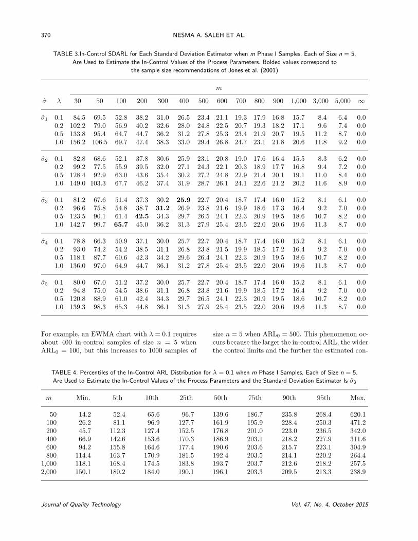
Although Jones et al.’s (2001) recommendationsregarding the amount of Phase I data were based onreducing the occurrence of early false alarms, theyalso provided practitioners with AARL values closeto ARL0 as shown in Table 2. However, the resultsin Table 3 show that these values of m are asso-ciated with large values of the SDARL. Account-ing for practitioner-to-practitioner variability in theARL reveals that the recommended amount of datais not nearly large enough to ensure that individualpractitioners will obtain an in-control ARL close tothe specified value. Additionally, our results suggestthat the larger the smoothing constant, the larger theSDARL will be for a given amount of data. For exam-ple, given m = 30, � = 0.1, and the process standarddeviation estimator �3, the in-control AARL = 133.9with SDARL = 81.2. If � increases to 0.5 and 1.0, thein-control AARL increases to 183.6 and 212.3 andthe corresponding SDARL increases as well to 123.5and 142.7, respectively. Recall that, when � = 1, theEWMA chart is equivalent to the Shewhart chart.Thus, we can conclude that Shewhart charts havehigher levels of between-practitioner variability thanthe EWMA chart.

Another aspect of control chart performance thatcan be seen from Table 3 is the e↵ect of the estima-tor of the process standard deviation on the controlchart performance. For a given value of � and smallm, EWMA charts based on the standard deviationestimator �4 have the smallest values of the SDARL.

In order to achieve stable in-control ARL perfor-mance when process parameters are estimated, therequired amount of Phase I data should yield an in-control AARL value close to ARL0 and an SDARLvalue that is su�ciently small. Zhang et al. (2014)


mss # 1932.tex; art. # 05; 47(4)


TABLE 2.In-Control AARL for Each Standard Deviation Estimator when m Phase I Samples, Each of Size n = 5,Are Used to Estimate the In-Control Values of the Process Parameters. Bolded values correspond to

the sample size recommendations of Jones et al. (2001)

m

� � 30 50 100 200 300 400 500 600 700 800 900 1,000 3,000 5,000 1

�1 0.1 134.9 147.4 163.7 176.9 182.9 186.4 188.7 190.3 191.5 192.4 193.2 193.8 197.7 198.6 199.90.2 153.4 162.8 175.2 184.9 189.2 191.6 193.1 194.2 195.0 195.6 196.1 196.5 198.9 199.5 200.30.5 186.9 187.8 191.6 194.9 196.4 197.2 197.7 198.0 198.3 198.5 198.6 198.7 199.5 199.7 199.91.0 216.7 208.2 203.5 201.6 201.0 200.8 200.6 200.5 200.4 200.3 200.3 200.3 200.1 200.0 200.0

�2 0.1 134.4 147.1 163.5 176.8 182.9 186.4 188.6 190.3 191.5 192.4 193.2 193.8 197.7 198.6 199.90.2 152.5 162.3 174.9 184.8 189.1 191.6 193.0 194.1 194.9 195.5 196.0 196.4 198.9 199.5 200.30.5 185.2 187.0 191.2 194.7 196.2 197.2 197.6 197.9 198.2 198.4 198.6 198.7 199.5 199.6 199.91.0 214.4 207.1 202.9 201.3 200.8 200.7 200.5 200.4 200.3 200.3 200.2 200.2 200.1 200.0 200.0

�3 0.1 133.9 146.8 163.3 176.7 182.8 186.3 188.6 190.2 191.4 192.4 193.1 193.7 197.7 198.6 199.90.2 151.6 161.7 174.6 184.6 189.0 191.4 193.0 194.1 194.9 195.5 196.0 196.4 198.9 199.5 200.30.5 183.6 186.1 190.7 194.5 196.1 196.9 197.5 197.8 198.1 198.3 198.5 198.6 199.5 199.6 199.91.0 212.3 206.0 202.4 201.0 200.7 200.5 200.4 200.3 200.2 200.2 200.2 200.1 200.0 200.0 200.0

�4 0.1 131.0 144.9 162.2 176.1 182.4 186.0 188.3 190.0 191.2 192.2 193.0 193.6 197.7 198.5 199.90.2 147.5 159.1 173.1 183.8 188.4 191.0 192.6 193.8 194.6 195.3 195.8 196.2 198.9 199.4 200.30.5 177.3 182.3 188.8 193.5 195.4 196.4 197.1 197.5 197.8 198.1 198.3 198.4 199.4 199.6 199.91.0 204.4 201.4 200.2 199.9 199.9 199.9 199.9 199.9 199.9 199.9 199.9 199.9 199.9 199.9 200.0

�5 0.1 132.4 145.9 162.7 176.4 182.6 186.1 188.5 190.1 191.3 192.3 193.1 193.7 197.7 198.6 199.00.2 149.6 160.4 173.9 184.2 188.7 191.2 192.8 193.9 194.7 185.4 195.9 196.3 198.9 199.4 200.30.5 180.4 184.2 189.7 194.0 195.7 196.7 197.3 197.7 198.0 198.2 198.4 198.5 199.4 199.6 199.91.0 208.3 203.7 201.3 200.5 200.3 200.2 200.1 200.1 200.1 200.1 200.1 200.0 200.0 200.0 200.0

suggested that an SDARL within 10% of the ARL0

may be reasonable, although still reflecting a signifi-cant amount of variation. Consequently, based on ourresults, a practitioner would need about 600 samplesof size n = 5 if � = 0.1, 700 if � = 0.2, 900 if � = 0.5,and 1000 if � = 1.0 to obtain SDARL values of nomore than 20 (10% of 200). These recommendationshold if any of the standard deviation estimators isused except for the estimator �1. If �1 is used, apractitioner would need a larger amount of Phase Idata; 700 samples of size n = 5 if � = 0.1, 800 if� = 0.2, and 1000 if � = 0.5 or 1.0. In most applica-tions, it will not be realistic to obtain this amount ofstable Phase I data from the process.

Tables 4, 5, and 6 provide practitioners with thein-control ARL percentiles for di↵erent values of m,of a fixed sample size n = 5 when (�, L) = (0.1,2.454), (0.2, 2.636), and (0.5, 2.777), respectively.

The values presented were calculated using 20,000simulated in-control ARL values when the processstandard deviation is estimated by �3. We also showthe minimum and maximum values obtained in oursimulations. These tables may help practitioners toassess the performance of their chart according totheir available amount of Phase I data.

Furthermore, we studied the required amount ofPhase I data of various values of the intended in-control ARL (ARL0). Tables 7–8 display the in-control AARL and SDARL values for di↵erent valuesof ARL0 when � = 0.1 and 0.5, respectively. The lastrow in each table, entitled m =1, refers to the casewhen the in-control process parameters are known.The bolded and italicized SDARL values in Tables7–8 are those that have an SDARL value within 10%of ARL0. As shown, the required number of sam-ples m increases with an increase in the ARL0 value.


mss # 1932.tex; art. # 05; 47(4)


TABLE 3.In-Control SDARL for Each Standard Deviation Estimator when m Phase I Samples, Each of Size n = 5,Are Used to Estimate the In-Control Values of the Process Parameters. Bolded values correspond to

the sample size recommendations of Jones et al. (2001)

m

� � 30 50 100 200 300 400 500 600 700 800 900 1,000 3,000 5,000 1

�1 0.1 84.5 69.5 52.8 38.2 31.0 26.5 23.4 21.1 19.3 17.9 16.8 15.7 8.4 6.4 0.00.2 102.2 79.0 56.9 40.2 32.6 28.0 24.8 22.5 20.7 19.3 18.2 17.1 9.6 7.4 0.00.5 133.8 95.4 64.7 44.7 36.2 31.2 27.8 25.3 23.4 21.9 20.7 19.5 11.2 8.7 0.01.0 156.2 106.5 69.7 47.4 38.3 33.0 29.4 26.8 24.7 23.1 21.8 20.6 11.8 9.2 0.0

�2 0.1 82.8 68.6 52.1 37.8 30.6 25.9 23.1 20.8 19.0 17.6 16.4 15.5 8.3 6.2 0.00.2 99.2 77.5 55.9 39.5 32.0 27.1 24.3 22.1 20.3 18.9 17.7 16.8 9.4 7.2 0.00.5 128.4 92.9 63.0 43.6 35.4 30.2 27.2 24.8 22.9 21.4 20.1 19.1 11.0 8.4 0.01.0 149.0 103.3 67.7 46.2 37.4 31.9 28.7 26.1 24.1 22.6 21.2 20.2 11.6 8.9 0.0

�3 0.1 81.2 67.6 51.4 37.3 30.2 25.9 22.7 20.4 18.7 17.4 16.0 15.2 8.1 6.1 0.00.2 96.6 75.8 54.8 38.7 31.2 26.9 23.8 21.6 19.9 18.6 17.3 16.4 9.2 7.0 0.00.5 123.5 90.1 61.4 42.5 34.3 29.7 26.5 24.1 22.3 20.9 19.5 18.6 10.7 8.2 0.01.0 142.7 99.7 65.7 45.0 36.2 31.3 27.9 25.4 23.5 22.0 20.6 19.6 11.3 8.7 0.0

�4 0.1 78.8 66.3 50.9 37.1 30.0 25.7 22.7 20.4 18.7 17.4 16.0 15.2 8.1 6.1 0.00.2 93.0 74.2 54.2 38.5 31.1 26.8 23.8 21.5 19.9 18.5 17.2 16.4 9.2 7.0 0.00.5 118.1 87.7 60.6 42.3 34.2 29.6 26.4 24.1 22.3 20.9 19.5 18.6 10.7 8.2 0.01.0 136.0 97.0 64.9 44.7 36.1 31.2 27.8 25.4 23.5 22.0 20.6 19.6 11.3 8.7 0.0

�5 0.1 80.0 67.0 51.2 37.2 30.0 25.7 22.7 20.4 18.7 17.4 16.0 15.2 8.1 6.1 0.00.2 94.8 75.0 54.5 38.6 31.1 26.8 23.8 21.6 19.9 18.5 17.2 16.4 9.2 7.0 0.00.5 120.8 88.9 61.0 42.4 34.3 29.7 26.5 24.1 22.3 20.9 19.5 18.6 10.7 8.2 0.01.0 139.3 98.3 65.3 44.8 36.1 31.3 27.9 25.4 23.5 22.0 20.6 19.6 11.3 8.7 0.0

For example, an EWMA chart with � = 0.1 requiresabout 400 in-control samples of size n = 5 whenARL0 = 100, but this increases to 1000 samples of

size n = 5 when ARL0 = 500. This phenomenon oc-curs because the larger the in-control ARL, the widerthe control limits and the further the estimated con-

TABLE 4. Percentiles of the In-Control ARL Distribution for � = 0.1 when m Phase I Samples, Each of Size n = 5,Are Used to Estimate the In-Control Values of the Process Parameters and the Standard Deviation Estimator Is �3

m Min. 5th 10th 25th 50th 75th 90th 95th Max.

50 14.2 52.4 65.6 96.7 139.6 186.7 235.8 268.4 620.1100 26.2 81.1 96.9 127.7 161.9 195.9 228.4 250.3 471.2200 45.7 112.3 127.4 152.5 176.8 201.0 223.0 236.5 342.0400 66.9 142.6 153.6 170.3 186.9 203.1 218.2 227.9 311.6600 94.2 155.8 164.6 177.4 190.6 203.6 215.7 223.1 304.9800 114.4 163.7 170.9 181.5 192.4 203.5 214.1 220.2 264.4

1,000 118.1 168.4 174.5 183.8 193.7 203.7 212.6 218.2 257.52,000 150.1 180.2 184.0 190.1 196.1 203.3 209.5 213.3 238.9


mss # 1932.tex; art. # 05; 47(4)




50 19.5 63.1 78.3 109.4 150.0 201.5 258.9 301.5 1,110.7100 36.0 93.7 109.1 136.4 168.9 206.0 245.5 271.6 527.7300 64.6 140.0 150.6 167.8 187.5 208.6 229.2 242.3 369.9500 95.5 155.6 163.4 176.7 191.9 208.1 223.2 233.0 304.4700 105.7 163.6 170.3 181.4 194.2 207.6 220.6 228.7 296.7

1,000 136.1 170.2 175.8 185.2 195.7 207.0 217.5 224.1 267.52,000 149.3 180.2 184.1 190.7 198.0 205.8 213.0 217.5 250.55,000 174.0 188.1 190.5 194.7 199.4 204.2 208.6 211.4 227.9



50 27.3 81.4 95.5 125.1 168.6 227.8 301.3 358.3 1,012.2200 71.0 133.9 144.4 164.2 189.7 219.8 251.4 272.1 487.1500 115.2 157.6 164.9 178.8 195.6 214.1 232.0 243.7 334.4700 125.1 163.9 170.7 182.5 196.9 212.2 227.0 236.6 314.0900 128.6 168.2 174.1 184.8 197.3 210.9 224.0 232.3 335.6

1,000 138.4 169.7 175.5 185.7 197.5 210.4 223.1 231.0 285.33,000 161.4 182.4 186.1 192.3 199.2 206.7 213.5 217.5 244.85,000 170.2 186.4 189.0 193.8 199.4 205.1 210.4 213.5 235.0

TABLE 7. In-Control AARL and SDARL Values for Di↵erent ARL0 for � = 0.1 when m Phase I Samples,Each of Size n = 5, Are Used to Estimate the In-Control Values of the Process Parameters and

the Standard Deviation Estimator Is �3

ARL0 = 100 ARL0 = 200 ARL0 = 370 ARL0 = 500(L = 2.148) (L = 2.454) (L = 2.702) (L = 2.815)

m AARL SDARL AARL SDARL AARL SDARL AARL SDARL

50 78.6 28.0 146.8 67.6 258.2 144.9 341.1 208.9100 86.0 20.8 163.3 51.4 290.2 111.2 384.6 160.4300 93.9 11.7 182.8 30.1 331.1 67.0 442.2 97.8400 95.2 10.0 186.3 25.9 338.8 57.7 453.4 84.4500 96.1 8.8 188.6 22.7 344.0 51.1 460.9 74.9600 96.7 7.9 190.2 20.4 347.7 46.1 466.3 67.7700 97.1 7.2 191.4 18.7 350.5 42.3 470.4 62.1800 97.4 6.7 192.4 17.4 352.7 39.2 473.6 57.7900 97.7 6.2 193.1 16.0 354.5 36.4 476.2 53.6

1,000 97.9 5.9 193.7 15.2 355.9 34.4 478.3 50.71,100 98.1 5.5 194.3 14.4 357.1 32.5 480.1 47.91 100.1 0.0 199.9 0.0 370.7 0.0 500.5 0.0


mss # 1932.tex; art. # 05; 47(4)



the Standard Deviation Estimator Is �3



50 93.1 37.0 186.1 90.1 347.1 196.5 470.4 285.9100 95.7 25.5 190.7 61.4 353.6 131.6 477.4 189.7500 98.9 11.1 197.5 26.5 365.7 56.3 493.3 80.8600 99.1 10.1 197.8 24.1 366.5 51.3 494.3 73.5700 99.2 9.4 198.1 22.3 367.0 47.4 495.0 68.0900 99.4 8.2 198.5 19.5 367.8 41.6 496.0 59.6

1,000 99.4 7.8 198.6 18.6 368.0 39.5 496.4 56.71,100 99.5 7.4 198.7 17.7 368.2 37.6 496.7 53.91,200 99.5 7.1 198.8 17.0 368.4 36.0 496.9 51.61,300 99.6 6.8 198.9 16.3 368.6 34.6 497.1 49.61 100.0 0.0 199.9 0.0 370.5 0.0 499.9 0.0

trol limits are in the tails of the distribution of thecontrol chart statistic. It is well-known that estimat-ing more extreme quantiles of a distribution requireslarger samples to achieve the same precision as whenestimating more central quantiles.

To study the e↵ect of the sample size n, we con-sidered the in-control AARL and SDARL values forn = 1 and n = 10. In each case, the control lim-its for 10,000 charts were estimated. Markov chainswere used to approximate the ARL for n = 10 andsimulation with 10,000 run lengths were used to es-timate each in-control ARL when n = 1. The resultsare given in Tables 9 and 10 for n = 10. We restrict

our attention to the two most e�cient estimators ofthe standard deviation. These tables show that thedata requirements, in terms of the total number ofobservations, are similar as for the case n = 5.

Tables 11 and 12 contain the in-control values ofAARL and SDARL for the EWMA chart when n = 1and the process standard deviation is estimated bythe moving-range estimator, defined as

MR =MR1.128

=1

1.1281

m� 1

mXi=2

|Xi �Xi�1|.

Again, as with n = 5 and n = 10, several thousandobservations are needed for the in-control SDARL

TABLE 9. In-Control AARL Values for the EWMA Chart with n = 10 and ARL0 = 200

m

� � 30 50 100 200 500 1,000 5,000 1

�3 0.1 129.8 143.8 161.7 175.7 188.2 193.4 198.5 200.00.2 143.6 156.4 171.7 183.0 192.3 196.1 199.3 200.00.5 168.4 176.5 186.0 192.0 196.6 198.1 199.5 200.01.0 192.5 193.8 196.6 198.3 199.3 199.8 199.9 200.0

�4 0.1 127.1 143.0 160.9 175.5 188.1 193.5 198.5 200.00.2 141.8 154.9 170.6 182.7 191.9 195.8 199.4 200.00.5 166.3 175.7 185.2 191.4 196.3 198.1 199.5 200.01.0 189.5 191.8 195.5 197.6 199.0 199.5 199.8 200.0


mss # 1932.tex; art. # 05; 47(4)


TABLE 10. In-Control SDARL Values for the EWMA Chart with n = 10 and ARL0 = 200

m

� � 30 50 100 200 500 1,000 5,000 1

�3 0.1 66.2 56.9 44.1 31.5 18.8 12.0 4.3 0.00.2 70.7 57.8 43.0 30.2 17.7 11.8 4.8 0.00.5 76.8 59.4 42.5 29.1 18.1 12.4 5.5 0.01.0 81.7 60.7 42.3 29.5 18.5 13.2 5.8 0.0

�4 0.1 64.5 56.5 43.8 31.6 18.4 11.8 4.3 0.00.2 69.7 57.4 42.7 30.0 17.8 11.7 4.8 0.00.5 75.3 59.3 42.2 29.1 18.0 12.6 5.5 0.01.0 79.7 60.0 42.6 29.5 18.5 13.0 5.8 0.0

values to be relatively small, say within 10% of thedesired in-control ARL value of 200. One has verylittle to no control over the in-control ARL value ifone follows the common recommendation of 25–50individual observations in Phase I. This result wasalso demonstrated by Saleh et al. (2015) for � = 1.

We also investigated the required number of PhaseI individual observations when changing the value ofthe desired in-control ARL for the EWMA chart. Ta-ble 13 and Table 14 contain our results when � = 0.1and � = 0.5, respectively. The bolded and italicizedvalues can be used to identify the number of obser-

vations required to have the SDARL value be within10% of the desired in-control ARL0 value. Highernumbers of observations are required for the largervalue of �. In addition, the required number of obser-vations increases as the desired value of the in-controlARL0 increases.

5. Adjusting the EWMAControl Limits

In order to overcome the problem of the oftenlow in-control ARL values when using estimated pa-rameters, Jones and Steiner (2012) and Gandy and

TABLE 11. In-Control AARL Values for the EWMA Chart with n = 1 and ARL0 = 200

m

� � 30 50 100 200 500 1,000 5,000 1

MR 0.1 248.5 192.6 183.6 184.0 194.1 196.8 199.0 200.00.2 352.6 247.7 212.0 201.6 199.8 199.4 200.3 200.00.5 721.0 365.1 258.0 223.9 208.8 204.9 200.5 200.01.0 976.4 458.8 275.0 233.5 210.1 206.3 200.3 200.0

TABLE 12. In-Control SDARL Values for the EWMA Chart with n = 1 and ARL0 = 200

m

� � 30 50 100 200 500 1,000 5,000 1

MR 0.1 2,061.0 234.7 123.3 80.6 51.3 33.0 15.1 0.00.2 1,517.5 439.9 181.8 100.4 60.0 40.8 17.9 0.00.5 3,833.3 1,228.1 307.8 144.8 75.1 48.4 21.9 0.01.0 5,622.3 1,301.7 299.9 159.3 79.1 54.7 22.9 0.0


mss # 1932.tex; art. # 05; 47(4)



the Standard Deviation Estimator Is MR



100 92.3 46.3 183.6 123.3 372.3 395.6 482.7 459.3250 95.2 27.4 189.1 69.9 349.5 165.1 474.4 246.8500 97.0 20.0 194.1 51.3 362.0 109.5 482.8 163.8

1,000 98.5 13.7 196.8 33.0 363.5 76.5 494.1 122.32,000 98.8 9.6 197.0 23.9 366.8 56.5 488.1 78.53,000 99.1 8.0 197.3 19.6 369.6 43.9 496.7 65.64,000 99.0 6.7 199.2 17.1 369.1 37.9 497.6 54.55,000 98.8 6.0 199.0 15.1 369.1 35.1 498.0 50.36,000 98.9 5.6 198.0 13.7 371.9 32.4 499.7 47.31 100.0 0.0 200.0 0.0 370.0 0.0 500.0 0.0

Kvaløy (2013) argued that determining the controllimits should be based on the conditional in-controlARL instead of the unconditional one. Their proposalwas to adjust the control limits in a way that guar-antees, with a suitably high prespecified probability,that the conditional in-control ARL meets or exceedsthe desired level.

Gandy and Kvaløy’s (2013) approach is based onbootstrapping the Phase I data to construct an ap-

proximate confidence interval for the control lim-its. The general bootstrap procedure, introduced byEfron (1979), is a resampling technique used to esti-mate the sampling distribution of any sample statis-tic. In quality-control applications, control charts de-signed based on bootstrap methods have been sug-gested as alternatives for the standard design meth-ods. See, for example, Bajgier (1992), Seppala et al.(1995), Liu and Tang (1996), and Jones and Woodall(1998). Recently, Chatterjee and Qiu (2009) prop-


the Standard Deviation Estimator Is MR



100 118.6 117.2 258.0 307.8 502.3 700.2 747.4 1,174.0250 104.6 45.9 226.2 132.5 416.4 286.9 563.5 365.4500 101.9 30.1 208.8 75.1 395.9 165.3 533.6 231.6

1,000 101.4 20.9 204.9 48.4 379.9 103.0 517.4 152.82,000 99.7 14.2 200.9 34.3 375.0 72.8 509.9 106.63,000 99.4 11.4 201.2 27.6 371.4 60.3 506.0 88.04,000 99.4 10.0 199.1 23.6 373.3 50.8 504.1 71.75,000 99.2 8.8 200.5 21.9 372.8 45.1 502.0 64.46,000 99.3 8.1 200.0 19.6 373.2 43.3 500.7 60.77000 99.5 7.7 200.2 18.4 370.9 37.1 500.2 49.11 100.0 0.0 200.0 0.0 370.0 0.0 500.0 0.0


mss # 1932.tex; art. # 05; 47(4)


osed estimating the control limits of the CUSUMchart using the bootstrap. Prior work on the boot-strap methods used in quality control focused on de-termining estimated control limits, not on controllingthe conditional ARL performance of control charts.

In order to best describe Gandy and Kvaløy’s(2013) approach, let us first define P as the true in-control distribution, P as the estimated in-controldistribution, ✓ = (µ,�) as the vector of process pa-rameters, ✓ = (µ, �) as the vector of estimated pro-cess parameters, and q as the control chart limit sat-isfying a specific in-control ARL. The quantities Pand ✓ are obtained from m in-control Phase I sampleseach of size n. The quantity q is a function of P and✓ or their estimates. For example, q(P, ✓) representsthe value of control limits conditioned on ✓ under thetrue in-control distribution P . For simplicity, in thisstudy, we evaluate a limit q for the absolute value ofthe EWMA chart statistic, defined in Equation (4),divided by the quantity

p�/(2� �). Therefore, the

control limit q that produces the desired in-controlARL is equal to the value of L defined in Equation(6).

When parameters are unknown, the observed con-trol chart performance depends on q(P, ✓), whichis unknown because P is unobservable. Gandy andKvaløy (2013) proposed using the estimator q(P , ✓)to build a lower one-sided confidence interval forq(P, ✓) using the bootstrap technique. Let (1�↵⇤)%be the percent of the in-control ARL values equal toor higher than the ARL0, then we can write

P (q(P , ✓)� q(P, ✓) > p↵⇤)= P (q(P, ✓) < q(P , ✓)� p↵⇤) = 1� ↵⇤, (9)

where p↵⇤ is a constant. The quantity p↵⇤ is unknownbecause it represents the (↵⇤) quantile of the un-observed sampling distribution of q(P , ✓) � q(P, ✓).Note that Gandy and Kvaløy (2013) incorrectly re-ferred to p↵⇤ as the (1 � ↵⇤) quantile. This wasa typographical error because it should be the ↵⇤

quantile. Gandy and Kvaløy (2013) proposed us-ing the bootstrap technique to estimate the distri-bution of q(P , ✓) � q(P, ✓) with the distribution ofq(P ⇤, ✓⇤)� q(P , ✓⇤), where P ⇤ and ✓⇤ = (µ⇤, �⇤) arethe estimated in-control distribution and process pa-rameters from the bootstrap samples, respectively.If B is the number of bootstrap samples, then p↵⇤

is approximated with p⇤↵⇤ , which represents the (↵⇤)quantile of [q(P ⇤i , ✓⇤i ) � q(P , ✓⇤i )], i = 1, 2, 3, . . . , B.The upper bound q(P , ✓)� p⇤↵⇤ is then taken as theadjusted control limit.

The simulation steps followed in our article are thesame as those listed in Gandy and Kvaløy (2013, p.651). In our simulation procedure, we used m = 50samples of size n = 5, ↵⇤ = 0.1, � = 0.1, B = 1,000bootstrap samples, and the process standard devia-tion estimator �3. We assumed, without loss of gen-erality, that the unknown true in-control distributionis N(0,

pn). We assumed that the desired in-control

ARL0 is 200. Because we found that the Shewhartchart has higher levels of between-practitioner vari-ability than the EWMA chart, we additionally de-signed it using this bootstrap approach. The samesimulation settings were used for the Shewhart chart.The procedure followed in calculating the controllimits, q(P , ✓), q(P ⇤i , ✓⇤i ), and q(P , ✓⇤i ), for each of theShewhart and EWMA control charts is discussed indetail in Appendix B. Once the limit (q(P , ✓)� p⇤↵⇤)was determined, the corresponding in-control andout-of-control ARLs were calculated. For the EWMAchart, the Markov chain approach described in Ap-pendix A was used in calculating the ARL.

Figures 2–3 contain the boxplots of the in-controland out-of-control ARL distributions, respectively,for the EWMA and Shewhart control charts. Forboth the EWMA and Shewhart charts, the limitscomputed with the bootstrap adjustment are indi-cated as “Adjusted Limits”. For reference, chartswith “Unadjusted Limits” were computed with m =50 samples of size n = 5 using (�, L) = (0.1, 2.454) forEWMA charts and L = 2.807 for Shewhart charts.The out-of-control ARL values were computed witha mean shift of � = 1, and the boxplots were con-structed from 2000 ARL values. In Figure 2, one cansee, as expected, that the adjusted limits resulted inabout 90% of the in-control ARL values for both theEWMA and Shewhart charts of at least 200 whencomputed using the bootstrap approach. Interest-ingly, more than 75% of the EWMA charts and 50%of the Shewhart charts with unadjusted limits hadan in-control ARL below 200, indicating a higher in-cidence of false alarms.

An interesting feature of Figure 2 is that theEWMA charts based on the bootstrap design havea much more variable in-control ARL distributionthan the charts based on unadjusted limits. Althoughthe in-control ARL distribution of the EWMA chartis extremely skewed to the right and more variablethan that of the unadjusted limits, the out-of-controlARL distribution of the EWMA chart with the ad-justed limits is very tight, as shown in Figure 3. TheEWMA design based on the bootstrap approach has


mss # 1932.tex; art. # 05; 47(4)


FIGURE 2. In-Control Distribution of the Conditional ARL when m = 50 and n = 5. The boxplots show the 5th, 10th,25th, 50th, 75th, 90th, and 95th percentiles of the conditional in-control ARL distribution.

a slightly more variable out-of-control ARL distri-bution than the standard design. The median out-of-control ARL is around 12 for the adjusted limitsand 9 for the unadjusted limits. This small loss inout-of-control performance comes with “guaranteed”in-control performance with 90% of the bootstrap ad-justed charts having in-control ARL values above 200as compared with only 25% of the charts with unad-justed limits. Although the increased variability inthe in-control ARL distribution of the EWMA chartsbased on the adjusted limits was initially surprisingto us, we quickly realized that we are not too con-cerned about charts with large in-control ARL values

as long as they can quickly detect an out-of-controlevent.

Another interesting feature of Figures 2 and 3 isthat the out-of-control ARL values of the Shewhartchart with the adjusted limits are considerably higherthan those of the EWMA chart with either adjustedor unadjusted limits. Hence, if the goal is to avoid fre-quent false alarms and to detect this sustained shiftquickly, then the EWMA chart remains much pre-ferred to the Shewhart chart.

Figure 4 shows the relationship between the in-control ARL values and the out-of-control ARL val-

FIGURE 3. Out-of-Control Distribution of the Conditional ARL when m = 50, n = 5, and a mean shift � = 1. The boxplotsshow the 5th, 10th, 25th, 50th, 75th, 90th, and 95th percentiles of the conditional out-of-control ARL distribution.


mss # 1932.tex; art. # 05; 47(4)


FIGURE 4. Scatterplot of the In-Control ARL Values vs. the Out-of-Control ARL Values of the EWMA Control ChartCategorized by the Mean Estimates Overestimating or Underestimating the Process Mean.

ues of the EWMA chart. The scatterplot presentsthe out-of-control ARL versus the in-control ARL,categorized by the standardized mean being under-estimated (< 0) or overestimated (� 0). The lowersmooth part of the scatterplot represents the casewhen the process mean is underestimated. Unexpect-edly, the high out-of-control ARL values are associ-ated with the lowest in-control ARL values. It canbe concluded from this figure that the increase inthe out-of-control ARL is due to overestimating theprocess mean rather than having a higher in-controlARL. Another point to note from Figure 4 is that apositive sustained shift along with an underestimatedin-control mean increases the e↵ective shift size and,as a consequence, results in a low out-of-control ARLvalue. Overestimating the in-control mean, on theother hand, leads to a decrease in the e↵ective shiftsize and, thus, a significant increase in the out-of-control ARL.

6. Concluding Remarks

In our article, we have extended the work of Joneset al. (2001) by using the SDARL metric in evaluat-ing the in-control performance of the EWMA con-trol chart when the parameters are estimated. Ac-counting for the practitioner-to-practitioner variabil-ity led to some quite di↵erent conclusions regard-ing the chart performance. First, the EWMA chartrequires more Phase I data than previously recom-mended in order to have consistent chart perfor-

mance among practitioners. Additionally, we foundthat charts designed with large values of the EWMAsmoothing constant have more variability in the ARLdistribution; thus, we recommend more Phase I databe used with larger smoothing constants. BecauseEWMA charts are typically used when quickly de-tecting small sustained shifts is of interest, the chartsare most often designed with small values of thesmoothing constant (� < 0.25).

With our recommendations regarding the requiredamount of Phase I data, we can easily see the di�-culty in controlling the in-control ARL value of anEWMA chart. We support the use of the bootstrap-based design approach of Jones and Steiner (2012)and Gandy and Kvaløy (2013), which was recentlyproposed for controlling the probability of the in-control ARL being at least a specified value. Our re-sults show that adjusting the EWMA control limitsaccordingly can result in a highly skewed in-controlARL distribution. However, such increases in thein-control ARL did not have much of an e↵ect onthe out-of-control performance of the chart. In ouropinion, this design approach is very promising andshould be considered while evaluating and compar-ing control charts. Controlling a percentile of thein-control ARL distribution can provide satisfactorychart performance among a wide range of practition-ers.

We found that, if one considers the necessary


mss # 1932.tex; art. # 05; 47(4)


amount of data for stable performance as determinedby the SDARL, fewer observations are required fordesigning an EWMA chart than a Shewhart chart.Thus, the EWMA chart, with a small smoothing con-stant, has an advantage over the Shewhart chart,which would require more Phase I data to achievesimilar stability in terms of ARL performance acrosssamples. Additionally, based on the bootstrap designprocedure, we found that the EWMA chart is muchpreferred to the Shewhart chart because, with theformer, one can simultaneously avoid too frequentfalse alarms and detect out-of-control sustained shiftsmore quickly.

Several competing process standard deviation es-timators were used as well in assessing the chartperformance. Among unbiased estimators, Jones etal. (2001) recommended the use of the estimator�3 = Spooled/c4(v + 1), and our results agree withthis recommendation. However, including the biasedestimators in the comparison, we find it preferableto use the estimator �4 = c4(v + 1)Spooled, espe-cially when only a small amount of Phase I data isavailable. Agreeing with Mahmoud et al. (2010), therange-based estimator was found to be the least ef-ficient compared with the other estimators, and wealso recommend against its use.

Appendix A:Calculating the AARL and SDARL

for the EWMA Chart with EstimatedParameters Using the Markov

Chain Approach

In our article, the EWMA chart is evaluated usingthe in-control AARL and SDARL metrics. The per-formance metrics were calculated using the Markovchain approach. Let h be the control limits given inEquation (6), t be the number of the subintervalsbetween the upper and lower control limits (namely,the number of transient states), and w be the widthof each subinterval defined as w = 2h/t. Saleh etal. (2013, Appendix B) derived the transition prob-abilities p`j , ` = 1, 2, . . . , t and j = 1, 2, . . . , t, forthe EWMA chart when process parameters are esti-mated. The probability p`j refers to the probabilityof moving from the transient state ` to the transientstate j. They calculated p`j using

p`j = '

✓Q

⇢Sj + w/2� (1� �)S`

�

�

� � +Zpm

��µ0, �0

◆

� '

✓Q

⇢Sj � w/2� (1� �)S`

�

�

� � +Zpm

��µ0, �0

◆,

where '(·) is the cumulative standard normal distri-bution function, the quantities Q and Z are definedin Equation (5), and S(·) represents the (·)th intervalmidpoint. We define R to be a t⇥ t matrix consist-ing of the probabilities of moving from one transientstate to another such that R = [p`j ], and u to bea t ⇥ 1 vector of ones. According to Markov chainapproach, the ARL vector is computed as

ARL = (I�R)�1u, (A.1)

where I is the identity matrix of dimension t ⇥ t.Here, ARL is a (t ⇥ 1) vector containing the ARLscorresponding to all the possible initial states. Wehave Y0 = 0. Hence, for an odd value of t, the (t +1)/2th element (middle element) corresponds to theARL satisfying this assumption. The ARL defined inEquation (A.1) is a function of the random variablesµ0 and �0, or more generally the random variables Qand Z. Hence, we can write the AARL as

AARL = E(ARL) =Z 1

0

Z 1

�1ARLgz(z)fQ(q)dzdq

(A.2)and the SDARL as

SDARL =⇥E(ARL2)� [E(ARL)]2

⇤1/2, (A.3)

where

E(ARL2) =Z 1

0

Z 1

�1ARL2gz(z)fQ(q)dzdq. (A.4)

Here, ARL is the element of the vector ARL corre-sponding to the initial state, and the gz(z) and fQ(q)are the probability density functions of the randomvariables Z and Q, respectively. Because the sam-ples are assumed to be i.i.d. normally distributed,the random variables Z and Q are independent. Thevariable Z follows the standard normal distribution,while Q follows a scaled chi (�) distribution. Saleh etal. (2013) provided the functional form of the proba-bility density function of Q for each of the standarddeviation estimator given in Equation (7). The inte-grations in Equations (A.2) and (A.4) were approx-imated using the Gaussian quadrature method. Thenumerical results were validated using Monte Carlosimulation.


mss # 1932.tex; art. # 05; 47(4)


Appendix B:Simplifying the Computations in

the Bootstrap Approach

In our article, we design the Shewhart and EWMAcontrol charts using the bootstrap approach. Westart here with providing the steps of applying Gandyand Kvaløy’s (2013) algorithm, then we list the cal-culation steps for each of the Shewhart and EWMAchart, along with providing some simplification rulesfor the Shewhart chart.

Gandy and Kvaløy’s Algorithm

The steps of Gandy and Kvaløy’s (2013) algorithmfor obtaining bootstrap-based control limits can besummarized as follows:

1. Without loss of generality, we let the true un-known in-control distribution P be N(0,

pn).

We generate a Phase I dataset of m sampleseach of size n from N(0,

pn) and compute µ

and �. We then compute the quantity q(P , ✓),where P = N(µ, �) is the estimated in-controldistribution and ✓ = (µ, �) is the estimate ofthe parameters that are used to run the chart.

2. We then generate B = 1000 bootstrap samplesfrom P and compute ✓⇤ = (µ⇤, �⇤) for each ofthe B samples. It is important to note that µ⇤

and �⇤ are calculated the same way as µ and �were calculated.

3. We finally compute the quantities q(P ⇤i , ✓⇤i ) andq(P , ✓⇤i ) for i = 1, 2, 3, . . . , B. We obtain thevalue of p⇤↵⇤ as the ↵ percentile of the bootstrapdistribution of q(P ⇤, ✓⇤) � q(P , ✓⇤). The final(adjusted) control limit for the chart is thentaken as q(P , ✓)� p⇤↵⇤ .

We generated the ARL distribution by repeating thesteps 1–3 for a number of times (we used 2000 times).Next, we explain in detail how to compute the di↵er-ent values of q for the Shewhart and EWMA charts.

Gandy and Kvaløy’s (2013) approach is based onthree limits; q(P , ✓), q(P ⇤i , ✓⇤i ), and q(P , ✓⇤i ). Thethree limits are defined as follows:

(a) The quantity q(P , ✓) represents the value ofL that produces the desired in-control ARLwhen the Phase II data are generated fromP = N(µ, �) and the limits are constructed us-ing ✓ = (µ, �).

(b) The quantity q(P ⇤i , ✓⇤i ), i = 1, 2, 3, . . . , B, rep-resents the value of L that produces the desired

in-control ARL when the Phase II data are gen-erated from P ⇤i = N(µ⇤i , �⇤i ) and the limits areconstructed using ✓⇤i = (µ⇤i , �⇤i ).

(c) The quantity q(P , ✓⇤i ), i = 1, 2, 3, . . . , B, rep-resents the value of L that produces the de-sired in-control ARL when the Phase II dataare generated from P = N(µ, �) and the limitsare constructed using ✓⇤i = (µ⇤i , �⇤i ).

Calculation of q for the Shewhart ControlChart

Consider the Shewhart control chart where thechart statistic is the sample mean (X) and the con-trol limits are µ±L(�/

pn), with L being the control-

limit constant chosen to satisfy a specific in-controlperformance. Finding the quantity q(P , ✓) impliesfinding L such that

P (µ� L�/p

n <X< µ + L�/p

n) = 1� ↵,

where ↵ is the false-alarm probability and X⇠N(µ, �/

pn). This can be simplified to

P

��X �µ

�/p

n

�� > L

!= P (|Z| > L) = ↵.

This follows that L = Z1�↵/2 or equivalentlyq(P , ✓) = Z1�↵/2. Similarly, q(P ⇤i , ✓⇤i ) = L =Z1�↵/2, i = 1, 2, 3, . . . , B. For Shewhart charts, ↵is the reciprocal of the in-control ARL. Thus, in ourstudy, ↵ = 0.005 and thus Z1�↵/2 = 2.807.

For the quantity q(P , ✓⇤i ), we need to find L suchthat

P (µ⇤i � L�⇤i /p

n <X< µ⇤i + L�⇤i /p

n) = 1� ↵,

where X⇠ N(µ, �/p

n) or equivalently

P

✓Z <

µ⇤i + L�⇤i /p

n� µ

�/p

n

◆

� P

✓Z <

µ⇤i � L�⇤i /p

n� µ

�/p

n

◆

= 1� ↵. (B.1)

In such a case, a search algorithm is required for find-ing the value of L that satisfies Equation (B.1). Thesearch algorithm could be of a binary search type orany other trial and error type. However, these meth-ods may take a long time to produce the results. Thuswe provide a short and a quick method for obtainingthe value of L.

Our studies showed that L is always bounded be-tween two values. Refer to the quantity in Equation


mss # 1932.tex; art. # 05; 47(4)


FIGURE B.1. Scatter Plot for Y and X Obtained Using Di↵erent Combinations of (µ, �, µ⇤, �⇤).

(B.1) as P (Z < b2) � P (Z < b1) = 1 � ↵. It can bededuced that, if µ⇤ � µ, then necessarily b1 � Z↵/2,which implies that L (�/�⇤)Z1�↵/2 + [

pn(µ⇤ �

µ)/�⇤]. Also, if µ⇤ µ, then necessarily b2 Z1�↵/2,which implies that L (�/�⇤)Z1�↵/2 + [

pn(µ �

µ⇤)/�⇤]. Hence, an upper bound for L can be definedas (�/�⇤)Z1�↵/2+(

pn|µ�µ⇤|/�⇤), where |·| denotes

the absolute value. Additionally, b2 � b1 > 2Z1�↵/2

because the symmetric interval is the shortest in-terval for a standard normal density containing agiven probability. Thus, substituting with the expres-sions of b1 and b2 and solving for L provides thatL � (�/�⇤)Z1�↵/2. Consequently, we can say thatL 2 (L1, L2), where

L1 =�

�⇤Z1�↵/2 and L2 = L1 + �, (B.2)

where � =p

n(|µ� µ⇤|/�⇤).

An important finding is that a very strong rela-tionship was found between the variables Y = L/L2

and X = �/L2. Figure B.1 is a scatterplot of 500observations of Y and X (obtained using di↵erentcombinations of µ, �, µ⇤, �⇤ and a search algorithmfor L).

Using a curve fitting technique, we found that acubic regression model between Y and X can fit thisrelationship almost perfectly. The best fit was foundto be related to the values of � and x. That is, if� < 0.626 and x < 0.08, then we use

y = 0.99985� 1.01234x + 4.48698x2 � 3.97727x3.

If � < 0.626 and x � 0.08, then we use

y = 1.00178� 1.09381x + 5.60924x2 � 8.95849x3.

Given the satisfaction of these conditions and theavailability of µ, �, µ⇤, and �⇤, we can find the valuesof L1, L2 and X and substitute into the fitted modelto obtain the value of L = yL2. The fitted modelsdo not provide accurate results for the case of � �0.626, but this case is uncommon. Consequently, if� � 0.626, a usual trial-and-error search algorithmis used to find the value of L that satisfies Equation(B.1).

So, for the Shewhart chart, we can summarize step3 of our algorithm as follows. Calculate � and x.If � < 0.626, use the appropriate fitted regressionmodel based on the value of x to find q(P , ✓⇤i ). Oth-erwise, we apply a search algorithm. An advantagefor having q(P , ✓) = q(P ⇤, ✓⇤) = Z1�↵/2 is that ad-justed limit can be reduced to be only taking the100(1�↵⇤)% percentile of q(P , ✓⇤i ), i = 1, 2, 3, . . . , B.

Calculation of q for the EWMA ControlChart

For the EWMA chart, finding the quantity q(P , ✓)is similar to the case of finding q(P, ✓); i.e., the valueof L that produces the desired in-control ARL whenthe in-control process parameters are known. Thisis because the in-control distribution is defined withthe same estimated parameters (✓) used in buildingthe control chart limits. Hence, it follows that q(P , ✓)


mss # 1932.tex; art. # 05; 47(4)


is equal to 2.454 for � = 0.1. Similarly, q(P ⇤i , ✓⇤i ) =2.454 for i = 1, 2, 3, . . . , B.

However, this result can’t be extended in findingthe quantity q(P , ✓⇤i ) because the estimates of thein-control distribution di↵er from that correspond-ing to the control limits. Hence, a search algorithmis required for finding the value of L satisfying an in-control ARL of 200. The search algorithm would be ofa trial-and-error type and should be associated witha validation technique (e.g., a Markov chain code) ineach and every iteration. It should be noticed that, ifthe Markov chain approach described in Appendix Ais used in the validation process, then the standard-ized sample mean W should be based on the quanti-ties Q = �⇤/�, ⌫i =

pn(Xi �(µ+�))/�, � =

pn�/�,

and Z =p

mn(µ⇤ � µ)/�.

This method can take a long time to produce re-sults. A similar simplifying rule to that of the Shew-hart chart can probably be used for the EWMAchart, but further investigation is needed to estab-lish this. As mentioned in the Shewhart chart case,we have the equality of q(P , ✓) and q(P ⇤, ✓⇤) and welet the adjusted limit be the 100(1�↵⇤)% percentileof q(P , ✓⇤i ), i = 1, 2, . . . , B.

References

Albers, W. and Kallenberg, W. C. M. (2004). “Are Es-timated Control Charts in Control?” Statistics 38(1), pp.67–79.

Aly, A. A.; Mahmoud, M. A.; and Woodall, W. H. (2015).“A Comparison of the Performance of Phase II Simple Lin-ear Profile Control Charts when Parameters are Estimated”.Communications in Statistics—Simulation and Computa-tion, to appear.

Bajgier, S. M. (1992). “The Use of Bootstrapping to Con-struct Limits on Control Charts”. In Proceedings of the De-cision Science Institute, pp. 1611–1613. San Diego, CA.

Chakraborti, S.; Human, S. W.; and Graham, M. A.(2009). “Phase I Statistical Process Control Charts: AnOverview and Some Results”. Quality Engineering 21(1), pp.52–62.

Chatterjee, S. and Qiu, P. (2009). “Distribution-Free Cu-mulative Sum Control Charts Using Bootstrap-Based Con-trol Limits”. The Annals of Applied Statistics 3(1), pp. 349–369.

Chen, G. (1997). “The Mean and Standard Deviation of the

Run Length Distribution of X Charts When Control Limitsare Estimated”. Statistica Sinica 7(3), pp. 789–798.

Crowder, S. V. (1987). “A Simple Method for Studying Run-Length Distributions of Exponentially Weighted Moving Av-erage Charts”. Technometrics 29(4), pp. 401–407.

Crowder, S. V. (1989). “Design of Exponentially WeightedMoving Average Schemes”. Journal of Quality Technology21(3), pp. 155–162.

Derman, C. and Ross, S. (1995). “An Improved Estimator

of � in Quality Control”. Probability in the Engineering andInformational Sciences 9(3), pp. 411–415.

Efron, B. (1979). “Bootstrap Methods: Another Look at theJackknife”. The Annals of Statistics 7(1), pp. 1–26.

Faraz, A.; Woodall, W. H.; and Heuchenne, C. (2015).“Guaranteed Conditional Performance of the S2 ControlChart with Estimated Parameters”. International Journalof Production Research 53(14), pp. 4405–4413.

Gandy, A. and Kvaløy, J. T. (2013). “Guaranteed Condi-tional Performance of Control Charts via Bootstrap Meth-ods”. Scandinavian Journal of Statistics 40, pp. 647–668.

Jensen, W. A.; Jones-Farmer, L. A.; Champ, C. W.; andWoodall, W. H. (2006). “E↵ects of Parameter Estimationon Control Chart Properties: A Literature Review”. Journalof Quality Technology 38(4), pp. 349–364.

Jones, L. A. (2002). “The Statistical Design of EWMA Con-trol Charts with Estimated Parameters”. Journal of QualityTechnology 34(3), pp. 277–288.

Jones, L. A.; Champ, C. W.; and Rigdon, S. E. (2001).“The Performance of Exponentially Weighted Moving Av-erage Charts with Estimated Parameters”. Technometrics43(2), pp. 156–167.

Jones, L. A.; Champ, C. W.; and Rigdon, S. E. (2004). “TheRun Length Distribution of the CUSUM with Estimated Pa-rameters”. Journal of Quality Technology 36(1), pp. 95–108.

Jones, L. A. and Woodall, W. H. (1998). “The Performanceof Bootstrap Control Charts”. Journal of Quality Technology30(4), pp. 362–375.

Jones, M. A. and Steiner, S. H. (2012). “Assessing the E↵ectof Estimation Error on the Risk-Adjusted CUSUM ChartPerformance”. International Journal for Quality in HealthCare 24(2), pp. 176–181.

Jones-Farmer, L. A.; Woodall, W. H.; Steiner, S. H.; andChamp, C. W. (2014). “An Overview of Phase I Analysis forProcess Improvement and Monitoring”. Journal of QualityTechnology 46(3), pp. 265–280.

Lee, J.; Wang, N.; Xu, L.; Schuh, A.; and Woodall, W. H.(2013). “The E↵ect of Parameter Estimation on Upper-SidedBernoulli Cumulative Sum Charts”. Quality and ReliabilityEngineering International 29(5), pp. 639-651.

Liu, R. Y. and Tang, J. (1996). “Control Charts for Depen-dent and Independent Measurements Based on the Boot-strap”. Journal of the American Statistical Association91(436), pp. 1694–1700.

Lucas, J. M. and Saccucci, M. S. (1990). “ExponentiallyMoving Average Control Schemes: Properties and Enhance-ments”. Technometrics 32(1), pp. 1–12.

Mahmoud, M. A.; Henderson, G. R.; Epprecht, E. K.; andWoodall, W. H. (2010). “Estimating the Standard Devia-tion in Quality Control Applications”. Journal of QualityTechnology 42(4), pp. 348–357.

Montgomery, D. C. (2013). Introduction to Statistical Qual-ity Control, 7th Edition. Hoboken, NJ: John Wiley & Sons,Inc.

Psarakis, S.; Vyniou, A. K.; and Castagliola, P. (2014).“Some Recent Developments on the E↵ects of ParameterEstimation on Control Charts”. Quality and Reliability En-gineering International 30(8), pp. 1113–1129.

Quesenberry, C. P. (1993). “The E↵ect of Sample Size on

Estimated Limits for X and X Control Charts”. Journal ofQuality Technology 25(4), pp. 237–247.

Roberts, S. W. (1959). “Control Chart Tests Based on Geo-metric Moving Averages”. Technometrics 1(3), pp. 239–250.


mss # 1932.tex; art. # 05; 47(4)


Robinson, P. B. and Ho, T. Y. (1978). “Average Run Lengthsof Geometric Moving Average Charts by Numerical Meth-ods”. Technometrics 20(1), pp. 85–93.

Saleh, N. A.; Mahmoud, M. A.; and Abdel-Salam, A.-S. G.(2013). “The Performance of the Adaptive ExponentiallyWeighted Moving Average Control Chart with EstimatedParameters”. Quality and Reliability Engineering Interna-tional 29(4), pp. 595–606.

Saleh, N. A.; Mahmoud, M. A.; Keefe, M. J.; andWoodall, W. H. (2015). “The Di�culty in Designing Shew-hart and X Control Charts with Estimated Parameters”.Journal of Quality Technology 47(2), pp. 127–138.

Seppala, T.; Moskowitz, H.; Plante, R.; and Tang, J.(1995). “Statistical Process Control via the Subgroup Boot-strap”. Journal of Quality Technology 27(2), pp. 139–153.

Simoes, B. F. T.; Epprecht, E. K.; and Costa, A. F. B.(2010). “Performance Comparisons of EWMA Control ChartSchemes”. Quality Technology and Quantitative Manage-ment 7(3), pp. 249–261.

Steiner, S. H. (1999). “EWMA Control Charts with Time-Varying Control Limits and Fast Initial Response”. Journalof Quality Technology 31(1), pp. 75–86.

Vardeman, S. B. (1999). “A Brief Tutorial on the Estimationof the Process Standard Deviation”. IIE Transactions 31(6),pp. 503–507.

Woodall, W. H. and Thomas, E. V. (1995). “Statistical Pro-cess Control with Several Components of Common CauseVariability”. IIE Transactions 27(6), pp. 757–764.

Zhang, M.; Megahed, F. M.; and Woodall, W. H. (2014).“Exponential CUSUM Charts with Estimated Control Lim-its”. Quality and Reliability Engineering International 30,pp. 275–286.

Zhang, M.; Peng, Y.; Schuh, A.; Megahed, F. M.; andWoodall, W. H. (2013). “Geometric Charts with EstimatedControl Limits”. Quality and Reliability Engineering Inter-national 29(2), pp. 209–223.

Zwetsloot, I. M.; Schoonhoven, M.; and Does, R. J. M.M. (2014). “A Robust Estimator for Location in Phase IBased on an EWMA Chart”. Journal of Quality Technology46(4), pp. 302–316.

Zwetsloot, I. M.; Schoonhoven, M.; and Does, R. J. M.M. (2015). “A Robust Phase I Exponentially Weighted Mov-ing Average Chart for Dispersion”. Quality and ReliabilityEngineering International. DOI: 10.1002/qre.1655

s


Documents

Another Look at the EWMA Control Chart with Estimated