Anomaly Detection of Time Series

Anomaly Detection of Time Series

A THESIS

SUBMITTED TO THE FACULTY OF THE GRADUATE SCHOOL

OF THE UNIVERSITY OF MINNESOTA

BY

Deepthi Cheboli

IN PARTIAL FULFILLMENT OF THE REQUIREMENTS

FOR THE DEGREE OF

Master Of Science

May, 2010

c© Deepthi Cheboli 2010

ALL RIGHTS RESERVED

Acknowledgements

First and foremost, I would like to thank my advisor, Prof.Vipin Kumar, for his valuable

support and help throughout the course of my Masters. I would like to thank the De-

partment of Computer Science and Engineering at University of Minnesota for providing

me excellent facilities during my graduate studies. I would like to acknowledge Varun

Chandola and Michael Steinbach for their valuable feedback for my work at all times.

I would also like to thank all the members of our Data Mining Group for providing a

challenging and friendly environment at work. I am indebted to my family members

and friends who have constantly motivated me all through my life and made me what

I am.

i

Abstract

This thesis deals with the problem of anomaly detection for time series data. Some of

the important applications of time series anomaly detection are healthcare, eco-system

disturbances, intrusion detection and aircraft system health management.

Although there has been extensive work on anomaly detection (1), most of the

techniques look for individual objects that are different from normal objects but do not

consider the sequence aspect of the data into consideration.

In this thesis, we analyze the state of the art of time series anomaly detection

techniques and present a survey. We also propose novel anomaly detection techniques

and transformation techniques for the time series data. Through extensive experimental

evaluation of the proposed techniques on the data sets collected across diverse domains,

we conclude that our techniques perform well across many datasets.

ii

Contents

Acknowledgements i

Abstract ii

List of Tables v

List of Figures vi

1 Introduction 1

1.1 Outline . . . . . . . . . . . . . . . . . . . . . . . . . . . . . . . . . . . . 2

2 Anomaly Detection for Time Series: A Survey 3

2.1 Applications . . . . . . . . . . . . . . . . . . . . . . . . . . . . . . . . . . 5

2.2 Problem setting . . . . . . . . . . . . . . . . . . . . . . . . . . . . . . . . 6

2.3 Challenges for Time Series Anomaly Detection . . . . . . . . . . . . . . 8

2.4 Types of Time Series data . . . . . . . . . . . . . . . . . . . . . . . . . . 9

2.5 Overview of Existing Techniques . . . . . . . . . . . . . . . . . . . . . . 11

2.6 Transformation of Data . . . . . . . . . . . . . . . . . . . . . . . . . . . 12

2.6.1 Aggregation . . . . . . . . . . . . . . . . . . . . . . . . . . . . . . 13

2.6.2 Discretization . . . . . . . . . . . . . . . . . . . . . . . . . . . . . 14

2.6.3 Signal Processing Based . . . . . . . . . . . . . . . . . . . . . . . 17

2.7 Detection Techniques . . . . . . . . . . . . . . . . . . . . . . . . . . . . . 18

2.7.1 Window Based . . . . . . . . . . . . . . . . . . . . . . . . . . . . 19

2.7.2 Proximity Based . . . . . . . . . . . . . . . . . . . . . . . . . . . 21

2.7.3 Prediction Based . . . . . . . . . . . . . . . . . . . . . . . . . . . 23

iii

2.7.4 Hidden Markov Models Based . . . . . . . . . . . . . . . . . . . . 28

2.7.5 Segmentation Based . . . . . . . . . . . . . . . . . . . . . . . . . 29

2.8 Discord Detection . . . . . . . . . . . . . . . . . . . . . . . . . . . . . . 33

2.9 Conclusions . . . . . . . . . . . . . . . . . . . . . . . . . . . . . . . . . . 35

3 Subspace based transformation for univariate timeseries 37

3.1 Motivation . . . . . . . . . . . . . . . . . . . . . . . . . . . . . . . . . . 37

3.2 Detecting Anomalies in Multivariate Time Series . . . . . . . . . . . . . 38

3.2.1 Subspace Monitoring for Multivariate Time Series . . . . . . . . 41

3.2.2 Converting a Multivariate Time Series to Univariate Time Series 42

3.3 Transformation . . . . . . . . . . . . . . . . . . . . . . . . . . . . . . . . 43

3.3.1 Methodology . . . . . . . . . . . . . . . . . . . . . . . . . . . . . 43

4 Experiments and Discussion 47

4.1 Anomaly Detection Techniques . . . . . . . . . . . . . . . . . . . . . . . 48

4.2 Data Sets Used . . . . . . . . . . . . . . . . . . . . . . . . . . . . . . . . 49

4.3 Comparison of Anomaly Detection Techniques . . . . . . . . . . . . . . 52

4.4 Comparison of Original and Transformed Time Series . . . . . . . . . . 54

4.5 Observations . . . . . . . . . . . . . . . . . . . . . . . . . . . . . . . . . 58

4.6 Conclusions and Future Work . . . . . . . . . . . . . . . . . . . . . . . . 61

5 Conclusions and Future Work 64

References . . . . . . . . . . . . . . . . . . . . . . . . . . . . . . . . . . . . . . 66

iv

List of Tables

4.1 Details of different univariate time series data sets used in the experiments. 50

4.2 Comparing results across all techniques. . . . . . . . . . . . . . . . . . . 54

4.3 Accuracy Results . . . . . . . . . . . . . . . . . . . . . . . . . . . . . . . 55

4.4 Accuracy Results for noisy data . . . . . . . . . . . . . . . . . . . . . . . 58

v

List of Figures

3.1 Windows of Univariate Time series . . . . . . . . . . . . . . . . . . . . . 39

3.2 Time series corresponding to normal and anomalous variables . . . . . . 40

3.3 Original and Transformed normal time series . . . . . . . . . . . . . . . 45

3.4 Original and Transformed Anomalous time series . . . . . . . . . . . . . 46

4.1 Average accuracies of original time series . . . . . . . . . . . . . . . . . . 56

4.2 Average accuracies of noise induced time series . . . . . . . . . . . . . . 57

4.3 Effect of Transformation on Scaled Time Series . . . . . . . . . . . . . . 62

vi

Chapter 1

Introduction

Anomalies are patterns in data that do not conform to a well defined notion of normal

behavior. The problem of finding these patterns is referred to as anomaly detection.

The importance of anomaly detection is due to the fact that anomalies in data translate

to significant and actionable information in a wide variety of application domains (1).

For example, an anomalous traffic pattern in a computer network could mean that a

hacked computer is sending out sensitive data to an unauthorized destination (2). An

anomalous MRI image may indicate the presence of malignant tumors (3) or anomalies

in credit card transaction data could indicate credit card or identity theft (4) . Detecting

anomalies has been studied by several research communities to address issues in different

application domains (1).

In many domains, such as flight safety, intrusion detection, fraud detection, health-

care, etc., data is collected in the form of sequences or time-series. For example, in

the domain of aviation or flight safety, the data collected from flights is in the form

of sequences of observations from various aircraft sensors during the flight. A fault

in the aircraft results in anomalous readings in sequences collected from one or more

of the sensors. Similarly, in health-care domain, an abnormal medical condition in a

patient’s heart can be detected by identifying anomalies in the time-series corresponding

to Electrocardiogram (ECG) recordings of the patient.

In this thesis, we identify different definitions of anomalies in time series. We focus

on a specific problem formulation, semi-supervised anomaly detection (1). We study

1

2

the relationship between the anomaly detection techniques and the nature of time se-

ries. Depending on this understanding we propose a novel transformation technique for

univariate time series which uses subspace based analysis.

1.1 Outline

This thesis is organized as follows.

• Chapter 2 is a survey on anomaly detection techniques for time series data.

It discusses the state of the art in this domain and categorizes the techniques

depending on how they perform the anomaly detection and what transfomation

techniques they use prior to anomaly detection.

• Chapter 3 discusses our novel subspace based transformation for univariate time

series data. It provides the motivation and methodology for this transformation.

• Chapter 4 provides the extensive experimental framework we developed and the

results obtained after transformation. We conclude with some observations and

future directions of research.

• Chapter 5 provides some discussions on various existing and proposed techniques

and we conclude with future directions of research.

Chapter 2

Anomaly Detection for Time

Series: A Survey

In this chapter we investigate the problem of anomaly detection for univariate time

series. Although there has been extensive work on anomaly detection (1), most of the

techniques look for individual objects that are different from normal objects but do

not consider the sequence aspect of the data into consideration. Such anomalies are

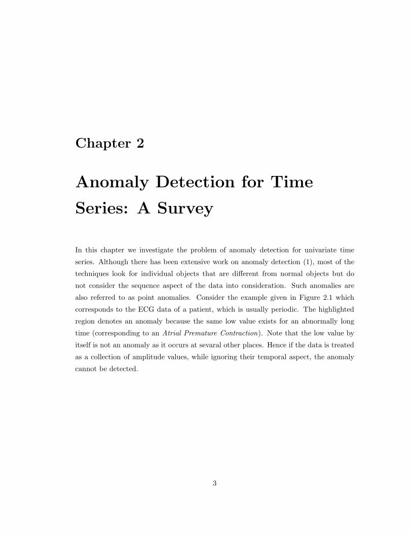
also referred to as point anomalies. Consider the example given in Figure 2.1 which

corresponds to the ECG data of a patient, which is usually periodic. The highlighted

region denotes an anomaly because the same low value exists for an abnormally long

time (corresponding to an Atrial Premature Contraction). Note that the low value by

itself is not an anomaly as it occurs at sevaral other places. Hence if the data is treated

as a collection of amplitude values, while ignoring their temporal aspect, the anomaly

cannot be detected.

3

4

0 500 1000 1500 2000 2500 3000−7.5

−7

−6.5

−6

−5.5

−5

−4.5

−4

Figure 2.1 : Anomalous time series

The problem of anomaly detection for time series is not as well understood as the

traditional anomaly detection problem. Multiple surveys: Chandola et al (1), Agyemang

et al (5) and Hodge et al (6) discuss the problem of anomaly detection. For symbolic

sequences, several anomaly detection techniques have been proposed. They are discussed

in a survey by Chadola et al (7). While for the univariate and multivariate time series,

limited number of techniques exist.

Existing research on anomaly detection for time series has been fragmented across

different application domains, without a good understanding of how different techniques

are related to each other and what their strengths and weaknesses are. The survey part

of this thesis is an attempt to provide a comprehensive understanding and structured

overview of the research on anomaly detection techniques for time series spanning multi-

ple research areas and application domains. We try to understand how the performance

of the techniques relates to the various aspects of the problem, such as nature of data,

nature of anomalies, etc.

The organization of the chapter is as follows. In Section 2.1 we discuss some of the

important applications of time series anomaly detection. Section 2.2 describes various

formulations for the problem of anomaly detection of time series and Section 2.3 deals

with the challenges involving this problem. We describe some of the different types of

5

time series data in section 2.4. In section 2.5 we give a brief overview of existing tech-

niques and categorize them into two orthogonal dimensions (a) the process of finding

anomalies (Procedural dimension, Section 2.7) and (b) the way the data is transformed

prior to anomaly detection (Transformation dimension, Section 2.6). Out of the three

problem formulations proposed in Section 2.2, we mainly deal with one of the formu-

lation called semi-supervised setting, in this survey. Section 2.8 gives a brief overivew

of another problem formulation called discord detection, which can be adapted to our

problem formulation.

2.1 Applications

Some of the important applications of time series anomaly detection are :

1. Detecting anomalous heart beat pulses using ECG data (8; 9) : Usually ECG

data can be seen as a periodic time series. An anomaly in this case would be the

non-conforming pattern e.g., in terms of periodicity or amplitude, which could

indicate a health problem.

2. Attack detection in recommender systems : Shilling attacks, in which the attackers

introduce biased ratings in order to influence future recommendations (10).

3. Detection of anomalous flight sequences using sensor data from aircrafts: Typical

system behavior of flights is characterized by the sensor data information of dif-

ferent parameters which change during the course of flight. Any deviation from

the typical system behavior us anomalous (11).

4. Shape anomalies : Finding the shapes which interestingly differ from others, where

each shape is converted to a time series (12; 13). In the field of medical data

mining, given several shapes of a species, a shape that differs from others might

indicate an anomaly caused by genetic mutation. In anthropological data mining,

different shapes of interest can be pottery, bones, arrowheads etc (14; 13).

5. Outlier light curves in catalogs of periodic stars : Detection of outliers in periodic

variable stars involves finding the statistical deviance from the rest. The out-

liers correspond to some interesting intrinsic physical differences, such as slowly

6

changing period or amplitude, which introduce noise in the light curve (15; 16).

6. Eco-system disturbances using earth science data such as vegetation or tempera-

ture (17).

2.2 Problem setting

The problem of anomaly detection for time series data can be viewed in different ways.

Here we discuss three possible definitions/settings.

Problem setting 1 : Detecting contextual anomalies in the time series.

In this setting of anomaly detection in a time series, the anomalies are the individual

instances of the time series which are anomalous in a specific context, but not otherwise.

This is a widely researched problem in the statistics community (18; 19; 20). Figure

2.2 shows one such example for a temperature time series which shows the monthly

temperature of an area over last few years. A temperature of 35F might be normal

during the winter (at time t1 ) at that place, but the same value during summer (at

time t2) would be an anomaly.

Monthly Temp

Time

Mar Jun Sept Dec Mar Jun Sept Dec Mar Jun Sept Dec

t2t1

Figure 2.2 : Contextual Anomaly at t2 in monthly temperature time series

7

Problem setting 2 : Detecting anomalous subsequence within a given time

series.

A different setting of the anomaly detection problem tries to find an anomalous subse-

quence with respect to a given long sequence (time series). Figure 2.1 is an example of

a time series containing an anomalous subsequence (the highlighted region), where in

the same low value exists for an abnormally long time, though the low value by itself is

not an anomaly as it occurs at several other places.

This problem corresponds to an unsupervised learning environment due to the lack

of labeled data for training, but most part of the long sequence (time series) is assumed

to be normal.

If the anomalous subsequence is of unit length, this problem is equivalent to finding

contextual anomalies in the time series, which is the problem setting 1.

The anomalous subsequences are also called discords. The concept of discords was

introduced by Keogh et al (21) in the context of finding anomalous subsequences within

a large time series : “Discords are the subsequences of a longer time series that are

maximally different from the rest of the sequence (22).”

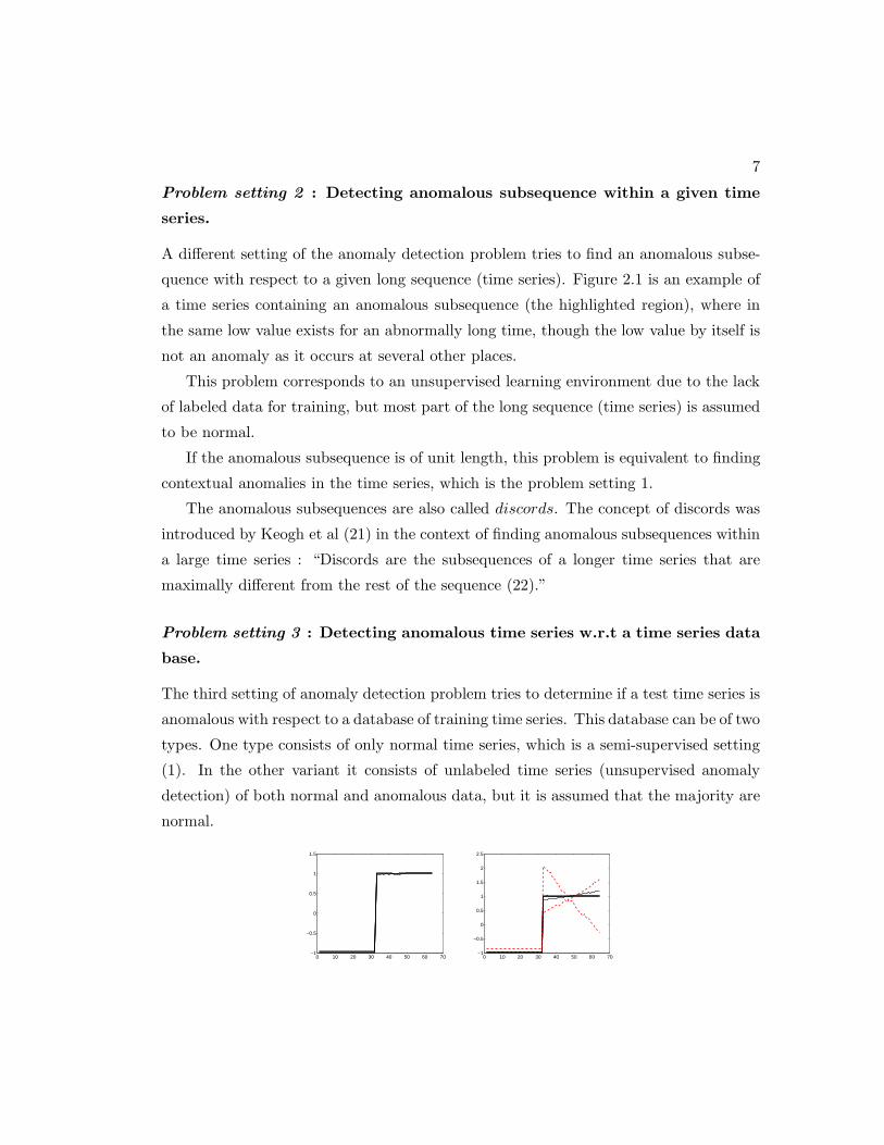
Problem setting 3 : Detecting anomalous time series w.r.t a time series data

base.

The third setting of anomaly detection problem tries to determine if a test time series is

anomalous with respect to a database of training time series. This database can be of two

types. One type consists of only normal time series, which is a semi-supervised setting

(1). In the other variant it consists of unlabeled time series (unsupervised anomaly

detection) of both normal and anomalous data, but it is assumed that the majority are

normal.

0 10 20 30 40 50 60 70−1

−0.5

0

0.5

1

1.5

0 10 20 30 40 50 60 70−1

−0.5

0

0.5

1

1.5

2

2.5

8

Figure 2.3 : Reference (left) and Test (right) time series for the NASA disk defect data

(23)

In this thesis, we are primarily going to discuss the semi-supervised problem setting.

Figure 2.3 shows one such example, where a set of reference time series (on the left)

correspond to measurements from a healthy rotary engine disk (23) and a test set of

time series (on the right) correspond to measurements from healthy (solid) and cracked

(dashed) disks. Detecting when an engine disk develops cracks is crucial.

The normal time series in the reference database and the anomalous ones can vary

among themselves due to one or more of following factors :

1. The normal time series are generated from a single generative process. The

anomalous time series are generated by a completely different generative process. The

generative process for normal time series might be periodic and the anomalous ones

differ from the periodic ones in this aspect.

2. The normal time series are generated from a single generative process. In the

anomalous time series, majority of the observations are generated by the same process,

but a few observations are generated by a different process.

Many anomaly detection algorithms discussed in this survey are suitable for all the

problem settings, but some are more specific to a particular setting.

2.3 Challenges for Time Series Anomaly Detection

Some major challenges associated with anomaly detection for time series are :

1. There are many ways in which an anomaly occurring in a time series may be

defined. An event within a time series may be anomalous; a subsequence within

a time series may be anomalous; or an entire time series may be anomalous with

respect to a set of normal time series.

2. For detecting anomalous subsequences, the exact length of the subsequence is

often unknown.

3. The training and test time series can be of different lengths.

9

4. Best similarity/distance measures which can be used for different types of time

series is not easy to determine. Simple measures like Euclidean distance do not

always perform well as they are highly sensitive to outliers and they also cannot

be used when the time series are of different lengths.

5. Performances of many anomaly detection algorithms are highly susceptible to noise

in the time series data, since differentiating anomalies from noise is a challenging

task.

6. Time series in real applications are usually long and as the length increases the

computational complexity also increases.

7. Many anomaly detection algorithms expect multiple time series to be at a com-

parable scale in magnitude while for most of the data it is not true.

2.4 Types of Time Series data

Most of the techniques in this survey use the training data to learn a model for normal

behavior and assign an anomaly score to a test time series based on the model. Thus

the performance of any technique depends on the nature of the normal time series as

well as the anomalous time series. The differences between normal and anomalous time

series are discussed in Section 2.2

We discuss two key characteristics of time series namely, periodicity and synchronous

nature. The combination of these properties would give 4 different kinds of time series.

We are given a dataset of n normal time series T = {t1, t2, . . . , tn} which can be viewed

as :

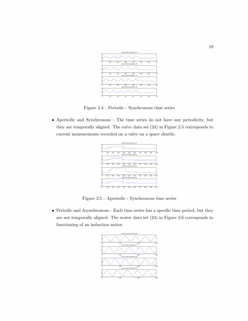
• Periodic and Synchronous : This is the simplest setting where every ti ǫ T has a

constant time period (p) and each of the time series are temporally aligned (start

from the same time instance). The power data set (24) in Figure 2.4 corresponds

to the weekly power usage by a research plant.

10

0 100 200 300 400 500 600 700−5

0

5power Normal Sequence #11

0 100 200 300 400 500 600 700−5

0


0 100 200 300 400 500 600 700−5

0


0 100 200 300 400 500 600 700−5

0


Figure 2.4 : Periodic - Synchronous time series

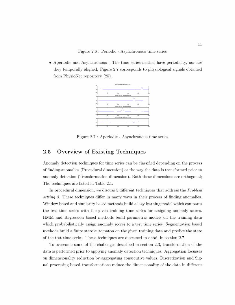
• Aperiodic and Synchronous : The time series do not have any periodicity, but

they are temporally aligned. The valve data set (24) in Figure 2.5 corresponds to

current measurements recorded on a valve on a space shuttle.

0 100 200 300 400 500 600 700 800 900 1000−5

0

5valve1 Normal Sequence #2

0 100 200 300 400 500 600 700 800 900 1000−5

0


0 100 200 300 400 500 600 700 800 900 1000−2

0


0 100 200 300 400 500 600 700 800 900 1000−5

0


Figure 2.5 : Aperiodic - Synchronous time series

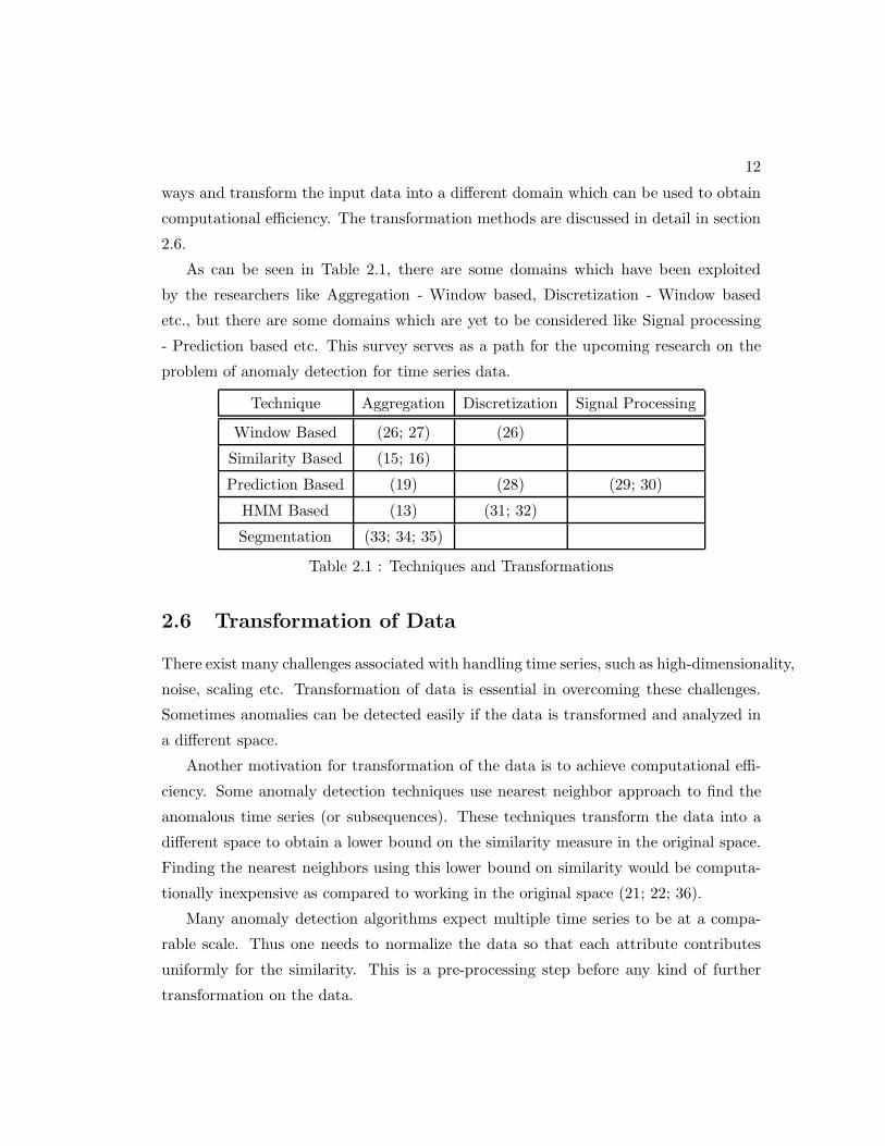
• Periodic and Asynchronous : Each time series has a specific time period, but they

are not temporally aligned. The motor data set (24) in Figure 2.6 corresponds to

functioning of an induction motor.

0 500 1000 1500−2

0

2motor1 Normal Sequence #19

0 500 1000 1500−2

0


0 500 1000 1500−2

0


0 500 1000 1500−2

0


11

Figure 2.6 : Periodic - Asynchronous time series

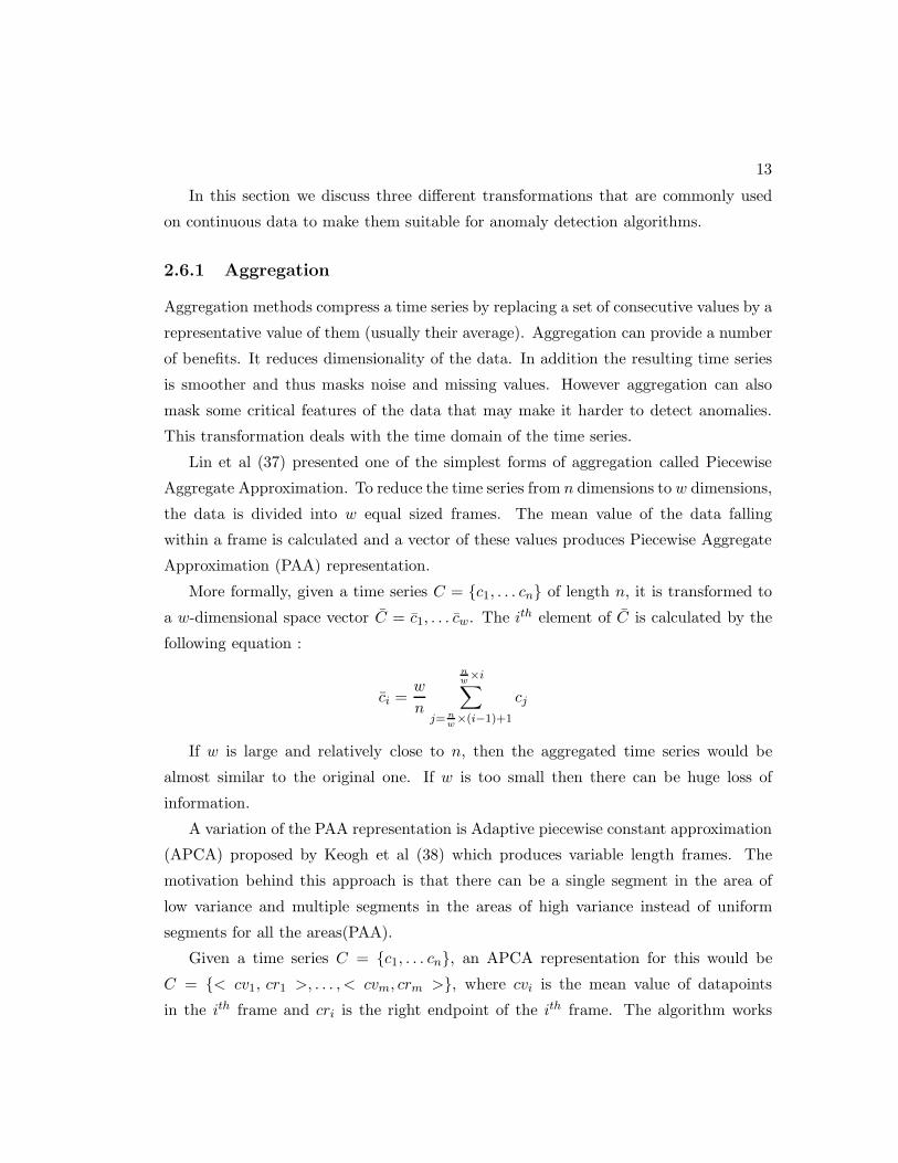
• Aperiodic and Asynchronous : The time series neither have periodicity, nor are

they temporally aligned. Figure 2.7 corresponds to physiological signals obtained

from PhysioNet repository (25).

0 50 100 150 200 250−10

0

10e0103 Normal Sequence #1201

0 50 100 150 200 250−10

0


0 50 100 150 200 250−10

0


0 50 100 150 200 250−10

0


Figure 2.7 : Aperiodic - Asynchronous time series

2.5 Overview of Existing Techniques

Anomaly detection techniques for time series can be classified depending on the process

of finding anomalies (Procedural dimension) or the way the data is transformed prior to

anomaly detection (Transformation dimension). Both these dimensions are orthogonal;

The techniques are listed in Table 2.1.

In procedural dimension, we discuss 5 different techniques that address the Problem

setting 3. These techniques differ in many ways in their process of finding anomalies.

Window based and similarity based methods build a lazy learning model which compares

the test time series with the given training time series for assigning anomaly scores.

HMM and Regression based methods build parametric models on the training data

which probabilistically assign anomaly scores to a test time series. Segmentation based

methods build a finite state automaton on the given training data and predict the state

of the test time series. These techniques are discussed in detail in section 2.7.

To overcome some of the challenges described in section 2.3, transformation of the

data is performed prior to applying anomaly detection techniques. Aggregation focusses

on dimensionality reduction by aggregating consecutive values. Discretization and Sig-

nal processing based transformations reduce the dimensionality of the data in different

12

ways and transform the input data into a different domain which can be used to obtain

computational efficiency. The transformation methods are discussed in detail in section

2.6.

As can be seen in Table 2.1, there are some domains which have been exploited

by the researchers like Aggregation - Window based, Discretization - Window based

etc., but there are some domains which are yet to be considered like Signal processing

- Prediction based etc. This survey serves as a path for the upcoming research on the

problem of anomaly detection for time series data.

Technique Aggregation Discretization Signal Processing

Window Based (26; 27) (26)

Similarity Based (15; 16)

Prediction Based (19) (28) (29; 30)

HMM Based (13) (31; 32)

Segmentation (33; 34; 35)

Table 2.1 : Techniques and Transformations

2.6 Transformation of Data

There exist many challenges associated with handling time series, such as high-dimensionality,

noise, scaling etc. Transformation of data is essential in overcoming these challenges.

Sometimes anomalies can be detected easily if the data is transformed and analyzed in

a different space.

Another motivation for transformation of the data is to achieve computational effi-

ciency. Some anomaly detection techniques use nearest neighbor approach to find the

anomalous time series (or subsequences). These techniques transform the data into a

different space to obtain a lower bound on the similarity measure in the original space.

Finding the nearest neighbors using this lower bound on similarity would be computa-

tionally inexpensive as compared to working in the original space (21; 22; 36).

Many anomaly detection algorithms expect multiple time series to be at a compa-

rable scale. Thus one needs to normalize the data so that each attribute contributes

uniformly for the similarity. This is a pre-processing step before any kind of further

transformation on the data.

13

In this section we discuss three different transformations that are commonly used

on continuous data to make them suitable for anomaly detection algorithms.

2.6.1 Aggregation

Aggregation methods compress a time series by replacing a set of consecutive values by a

representative value of them (usually their average). Aggregation can provide a number

of benefits. It reduces dimensionality of the data. In addition the resulting time series

is smoother and thus masks noise and missing values. However aggregation can also

mask some critical features of the data that may make it harder to detect anomalies.

This transformation deals with the time domain of the time series.

Lin et al (37) presented one of the simplest forms of aggregation called Piecewise

Aggregate Approximation. To reduce the time series from n dimensions to w dimensions,

the data is divided into w equal sized frames. The mean value of the data falling

within a frame is calculated and a vector of these values produces Piecewise Aggregate

Approximation (PAA) representation.

More formally, given a time series C = {c1, . . . cn} of length n, it is transformed to

a w-dimensional space vector C = c1, . . . cw. The ith element of C is calculated by the

following equation :

ci =w

n

nw×i∑

j= nw×(i−1)+1

cj

If w is large and relatively close to n, then the aggregated time series would be

almost similar to the original one. If w is too small then there can be huge loss of

information.

A variation of the PAA representation is Adaptive piecewise constant approximation

(APCA) proposed by Keogh et al (38) which produces variable length frames. The

motivation behind this approach is that there can be a single segment in the area of

low variance and multiple segments in the areas of high variance instead of uniform

segments for all the areas(PAA).

Given a time series C = {c1, . . . cn}, an APCA representation for this would be

C = {< cv1, cr1 >, . . . , < cvm, crm >}, where cvi is the mean value of datapoints

in the ith frame and cri is the right endpoint of the ith frame. The algorithm works

14

by first converting the problem into a wavelet compression problem, for which there

are well known optimal solutions, and then converting the solution back to the APCA

representation.

The drawback of this approach is that the obtained time series is no longer in the

standard format. A value in the output time series can correspond to varying number of

events in the original time series or just one instance value. Thus this transformation is

not yet used in any of the traditional anomaly detection algorithms, since they cannot

deal with the non-uniformity of the time series.

2.6.2 Discretization

The primary goal of discretization is to convert the given time series into a discrete

sequence of finite alphabets. This transformation deals with the amplitude domain

of the time series. Primary motivation behind discretization is to utilize the existing

symbolic sequence anomaly detection algorithms (39; 37). Another motivation is to

improve the computational efficiency (21; 22; 36). However discretization can also

cause loss of information.

Discretization involves the following steps : (i) Divide the amplitude range (max-

min) of the time series into different bins (ii) Assign a symbol to each of the bin which

can be an alphabet or an integer etc. (iii) Transform the time series by replacing every

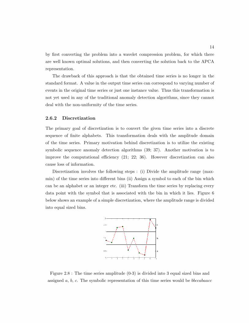
data point with the symbol that is associated with the bin in which it lies. Figure 6

below shows an example of a simple discretization, where the amplitude range is divided

into equal sized bins.

Figure 2.8 : The time series amplitude (0-3) is divided into 3 equal sized bins and

assigned a, b, c. The symbolic representation of this time series would be bbccabaacc

15

The discretization techniques vary according to how the bins and symbols are chosen.

Let us consider the variants in terms of symbols. Choices for the symbols can either

be integers or alphabets. Although the use of unordered alphabets is quite common

(37; 22), the use of integers retains more information. For example if integers 1, 2, 3

are used in the place of a, b, c in the example of Figure 2.8, one could easily determine

that the data points in bin c (integer 3) are closer to bin b (integer 2) than to bin a

(integer 1), which is not possible if unordered alphabets are used.

Forrest and DasGupta (40) discuss a discretization scheme that makes use of integers.

They number the bins using integers and then encode them into a binary form. Each

bin is thus associated with a binary number. Now each data point is given a binary

symbol depending on the bin where it falls. The 2 bins with all 0’s and all 1’s is not

considered during training so that the observations of the test time series which fall

outside the range of training time series are mapped to them depending on which side

of the range they cross. Thus there are 2m − 2 bins for m bits.

There are number of ways in which the intervals can be chosen. In the following, we

discuss three ways in which this can be done :

1. Equal bin size :

The amplitude range can be divided into n equal bins and each bin is assigned a unique

symbol. Figure 2.8 provides an illustration.

2. Equal frequency :

The amplitude range is divided into bins such that each bin has equal number of data

points (37).

3. Clustering :

The amplitude range is divided into different bins such that each bin has closely related

values and thus a unique discrete symbol can be assigned to each bin (41).

One of the most widely used discretization technique called SAX (Symbolic Ag-

gregate approXimation) (37) uses the Piecewise Aggregate Approximation discussed in

16

2.6.1 followed by equal frequency binning. The advantage of this method over many dis-

cretization techniques is that it is the only one that allows both dimensionality reduction

and lower bounding of Lp norms (distance measures) (21; 22; 36).

If the data distribution is known, equal frequency binning can be seen as the division

of this distribution into equal sized areas. Since the time series are normalized before

PAA, they tend to have a highly Gaussian distribution. In SAX transformation, a

notion called breakpoints is introduced which divide the gaussian into equal-sized areas.

Breakpoints are a sorted list of numbers B = β1, . . . βα−1 such that the area under a

N(0, 1) Gaussian curve from βi to βi+1 = 1/α.

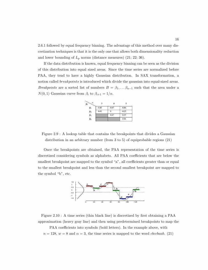
Figure 2.9 : A lookup table that contains the breakpoints that divides a Gaussian

distribution in an arbitrary number (from 3 to 5) of equiprobable regions (21)

Once the breakpoints are obtained, the PAA representation of the time series is

discretized considering symbols as alphabets. All PAA coefficients that are below the

smallest breakpoint are mapped to the symbol “a”, all coefficients greater than or equal

to the smallest breakpoint and less than the second smallest breakpoint are mapped to

the symbol “b”, etc.

Figure 2.10 : A time series (thin black line) is discretized by first obtaining a PAA

approximation (heavy gray line) and then using predetermined breakpoints to map the

PAA coefficients into symbols (bold letters). In the example above, with

n = 128, w = 8 and α = 3, the time series is mapped to the word cbccbaab. (21)

17

Discussion:

Though transformation of the continuous data to discrete/segmented form helps there

exist a lot of discretization techniques which have some basic drawbacks with them.

Firstly, the dimensionality of the symbolic representation is the same as the original data

after some transformations, which is a challenge for the anomaly detection algorithms.

Secondly, although some distance measures can be defined on the symbolic sequences,

these measures do not correlate well with the distance measures of the original time

series. Finally, many approaches need access to the entire data for the creating the

representation.

2.6.3 Signal Processing Based

Sometimes anomalies can be detected more easily if the data is used in a different space.

Signal processing techniques like Fourier transforms, wavelet transforms help to obtain

this entirely different space of coefficients where the data can be analyzed (42; 29).

These techniques are also used to get a lower dimensional representation of time series.

Many of these transformations are useful in achieving lower bounding of norms, in order

to make the algorithm computationally efficient (43; 44).

One such signal processing technique that has been used in the context of anomaly

detection for time series data is Haar Transform. A 1-dimensional vector (x0, x1) is

transformed as (s0, s1) by Haar transform, using

(s0 s1)T = D(x0 x1)

T, where D =

1√2

(

1 1

1 −1

)

It can be seen that s0, s1 are the sum and difference of x0, x1 and scaled by 1√2

to preserve energy. In general Haar transform can be seen as a sequence of averaging

and differencing operations on the consecutive values of a discrete time function. This

transformation preserves the Euclidean distance between two time series and is therefore

a useful technique for compression. If a prefix of the transformed time series is considered

instead of the entire sequence, the Euclidean distance between these prefixes will be

the lower bounding estimate of the actual Euclidean distance. Since the distance is

preserved even after the transformation, these prefixes which have lower dimension than

18

the original time series, can be considered for the anomaly detection problem and hence

get a better computational time. These lower bounding estimates are clearly discussed

by Chan et al (45).

Shahabi et al. (46; 47) proposed a wavelet-based data structure called TSA-Tree

to efficiently retrieve trends and surprises in spatio-temporal data. The wavelet based

approaches tend to outperform the other methods : DFT and SVD, since these methods

only consider the frequency components of the time series, where as wavelets process

the data at different resolutions.

Ma et al (27) use one class SVMs for prediction which need a set of vectors as input

instead of a time series. Thus they convert the time series into a phase-space using

time-delay embedding process, i.e., create overlapping subsequences from a given long

sequence. These vectors are projected into an orthogonal subspace which acts as a high

pass filter used to filter out the low frequency components and allow only high frequency

ones (anomalies).

2.7 Detection Techniques

The discussion in the previous sections provided understanding on how the time series

look and how they can be transformed for the application of anomaly detection tech-

niques. This section discusses the various anomaly detection techniques, some of which

have been proposed and evaluated in the literature, many others are new or slight vari-

ations of the existing techniques, to suit the Problem setting 3 mentioned in section 2.2.

In general, the process of anomaly detection consists of the following steps :

1. Compute the anomaly scores of individual observations or subsequences of a given

test time series using a detection technique.

2. Aggregate these anomaly scores to calculate the anomaly score of the given test

time series. This aggregation can be done in different ways, for example : (1)

mean of all the anomaly scores, (2) mean of top k anomaly scores (3) mean of log

of anomaly scores (4) number of times the running average of the anomaly scores

exceeds a threshold etc.

A test time series with anomaly score greater than a threshold is labeled anomalous.

19

2.7.1 Window Based

The techniques in this category divide the given time series into fixed size windows

(subsequences) to localize the cause of anomaly within one or more windows. The

motivation behind this technique is that an anomaly in a time series can be caused due

to the presence of one or more anomalous subsequences.

Window based techniques (26) extract fixed length (= m) windows (subsequences)

from training and test time series by moving one or more symbols (hop) at a time. The

anomaly score of a test time series is calculated by aggregating the anomaly scores of

its windows. A formal description of a generic window based scheme is as follows :

1. Given a training database, Straining = {S1, S2 . . . , Sn}, extract p windows of each

time series Si , si1, si2, . . . sip , where p can be calculated as |Si| + m − 1 when

sliding a window of size m, one step at a time. Similarly for the test database

Stest = {T1, T2, . . . , Tn}, divide each test time series Ti into |Ti| + m − 1 windows

, ti1, ti2 , . . . tip′.

2. The anomaly score for each test window (A(tij )) is calculated using its similarity

to the training windows. This similarity function can be distance measures like

Euclidean, Manhattan or Correlation values, etc.

If the subsequences are obtained by sliding one step at a time, considering all possible

overlaps, it gets computationally inefficient since the number of windows is nearly equal

to the length of the time series. Hence one alternative to obtain the subsequences is

to slide a window of fixed length (m) across the time series and move it with a certain

hop (h) each time, that is skip h observations from the initial position of the current

window and start the next window. A special case would be hgeqm, where there is

no overlap between the windows. The disadvantage of the hop being too large is that

there can be some loss of information. For an appropriate value of window size m, if

h = 1 then the probability that the anomaly is captured by atleast one window is 1, but

when h > 1 this probability might reduce. Consider the training database containing n

similar time series abcabcabc, where each symbol is a real value. If the window size is 3,

the training windows for any value of h would include only the following subsequences

: abc, bca, cab. Let a test time series be abccabcabc, where the occurrence of c after the

20

first abc is anomalous. Table 2.2 shows the test windows generated with different values

of hop.

hop (h) Windows

1 abc, bcc, cca, cab, abc, bca, cab, abc

2 abc, cca, abc, cab

3 abc, cab, cab

4 abc, abc

Table 2.2 : Windows of size 3 for different hop values

Both h = 1, 2 capture the anomalous occurrence of c by the windows bcc and cca

as there will not be any neighbors of these among the training windows. Hops of 3, 4

fail to capture anomaly as they miss the c during the window shift. Thus the value of

h has to be carefully chosen.

The window based techniques can differ in their score assignment to a test window.

For example, the anomaly score of a test window can be the distance to its kth nearest

neighbor among the training windows (26). Ma et al (27) use the training windows to

build one class SVMs for classification. The anomaly score of a test window is 0 or 1

depending on whether it is classified as normal or anomalous using the trained SVM.

Once the windows are extracted from the training and test time series, one can apply

any traditional anomaly detection technique for multivariate data to assign an anomaly

score to each window of the test time series (1).

Strengths and Weaknesses : The drawback of window based techniques is that

the window size has to be chosen carefully so that it can explicitly capture the anomaly.

The optimal size of the window depends on the length of the anomalous region in

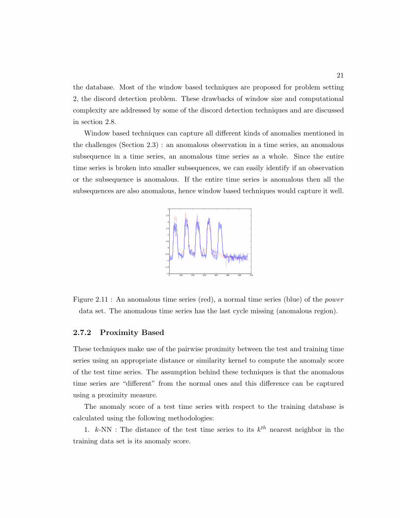
the anomalous time series. For example, in the power data set in Figure 2.11, the

anomalous region has the same length as the periodicity of the time series. Thus if m

is chosen to be smaller than the cycle length, the performance will be poor, while the

performance will improve if m is larger than the cycle length. Another drawback of

window based techniques is that they are computationally expensive. Since every pair

of test and training windows are compared, the complexity is O((nl)2), where l is the

average length of the time series, n is the number of test and training time series in

21

the database. Most of the window based techniques are proposed for problem setting

2, the discord detection problem. These drawbacks of window size and computational

complexity are addressed by some of the discord detection techniques and are discussed

in section 2.8.

Window based techniques can capture all different kinds of anomalies mentioned in

the challenges (Section 2.3) : an anomalous observation in a time series, an anomalous

subsequence in a time series, an anomalous time series as a whole. Since the entire

time series is broken into smaller subsequences, we can easily identify if an observation

or the subsequence is anomalous. If the entire time series is anomalous then all the

subsequences are also anomalous, hence window based techniques would capture it well.

0 100 200 300 400 500 600 700−2

−1.5

−1

−0.5

0

0.5

1

1.5

2

2.5

3

Figure 2.11 : An anomalous time series (red), a normal time series (blue) of the power

data set. The anomalous time series has the last cycle missing (anomalous region).

2.7.2 Proximity Based

These techniques make use of the pairwise proximity between the test and training time

series using an appropriate distance or similarity kernel to compute the anomaly score

of the test time series. The assumption behind these techniques is that the anomalous

time series are “different” from the normal ones and this difference can be captured

using a proximity measure.

The anomaly score of a test time series with respect to the training database is

calculated using the following methodologies:

1. k-NN : The distance of the test time series to its kth nearest neighbor in the

training data set is its anomaly score.

22

2. Clustering : The training time series are clustered into a specified number of

clusters and the cluster centroids are computed. The distance of the test time series to

its closest cluster centroid is its anomaly score.

The similiarity based techniques primarily differ in the choice of similarity measures

for the calculation of anomaly score. Different similarity/distance measures can be

adopted such as correlation, Euclidean, Cosine, DTW etc.

Simple measures like Euclidean, though are well understood and are faster to com-

pute, they cannot be used when the time series are of different lengths. Also, consider

the physiological signals in Figure 2.7 which are all normal, but they have the spikes

at different time stamps. These time series are non-linearly aligned which is one of the

challenges in handling time series data. Euclidean distance measure would give high

anomaly score to these time series in case of similarity based techniques.

Dynamic time warping (DTW) (48) is a distance measure which is more suitable

for comparing time series which are non-linearly aligned or of different lengths. DTW

aligns the time series which are similar but with small variations in the time axis in such

a way that the distance between them is minimal. This minimal distance can be used

to characterize the similarity between the time series. The disadvantage of DTW is it

performs excessive matchings which can make the algorithm computationally expensive

and can also lead to distortion of the actual distance between time series.

Another challenge with time series data is that different time series can be generated

at different conditions and times and hence they may not be synchronous. Hence,

measures like Euclidean and DTW may consider two phase misaligned time series to

be dissimilar though they are almost similar. For example, consider the motor data set

in Figure 2.6, where all the time series are normal but they are not in phase (phase-

misaligned). While DTW addresses the issue of non-linear alignment of the time series,

Cross Correlation, a similarity measure, addresses the issue of phase mis-alignments

(15). Given two time series, different phase-shifts of the pair are considered and the

correlation between them for each alignment is computed. The maximum of these

correlations is used as the cross correlation measure for these two time series. Thus,

two time series with phase misalignments will have high correlation in one of their

phase-shifted alignments, which shows that they have high similarity. Revisiting the

motor data set in Figure 2.6, the first two time series will have maximum correlation

23

when one of them is considered with a π2 phase shift.

Anomaly detection techniques in this category include a k-nearest neighbor based

anomaly detection technique, which has been proposed by Propotopapas et al (15) to

compare catalogs of periodic light curves to obtain the anomalies. They handle the issues

of phase-misaligned data using cross correlation measure which is computed efficiently

in Fourier space using convolution theorem.

For the same problem of comparing periodic light-curves, Rebba Pragada et al (16)

use PCAD (Periodic Curve Anomaly Detection) clustering algorithm which is a variant

of k-means. The similarity of the test time series is a function of maximum cross

correlation measure between the time series and the cluster centroids obtained from

PCAD.

Strengths and Weaknesses : The drawbacks of similarity based techniques are

that, they can determine if the entire time series is anomalous or not, but cannot

exactly locate the anomalous subsequence. To localize the exact region(s) within the

time series which causes the anomaly, one needs to do post processing of the time

series. Also the phase misalignments and the non-linear alignments of different time

series, which are some common challenges for the time series data, restrict the usage

of different proximity measures for these class of techniques. Thus the performance of

these techniques is highly dependent on the proximity measure, which is often not easy

to choose. In detecting different types of anomalies, similarity based techniques might

fail when a single observation is anomalous in the time series as its effect might not be

prominent when the entire time series is considered at once.

These techniques would detect anomalies such as anomalous subsequences in a time

series or an anomalous time series as a whole.

2.7.3 Prediction Based

Anomaly detection using predictive models has been mostly investigated in the statistics

community (49; 50; 18), most of which look for single observations as outliers. The

motivation behind these techniques is that the normal time series are generated from

a statistical process and the anomalous time series do not fit this process. So the key

step is to learn the parameters of this process from the training database of normal time

24

series and then estimate the probability that a test time series is generated from the

learnt process.

A basic predictive model based anomaly detection technique consists of the following

steps (26):

1. Learn a predictive model on the given training time series, which uses m obser-

vations (history) to predict the (m + 1)th observation following them.

2. For a test time series, using the predictive model built in step 1, forecast the ob-

servation at each time step using the observations seen so far (previous m observations).

The prediction error corresponding to an observation is a function of the difference be-

tween the forecasted value and the actual observation and certain model parameters

such as the variance of the model.

The techniques differ in the prediction models used and can be broadly categorized

as follows.

1. Time series based models such as Moving Average (MA) (51), AutoRegression

(AR) (52; 51), ARMA (53), ARIMA (54), Kalman filters (55) etc. The input

to these models is the entire time series and the length of the history (m), also

denoted as the order of the model. These models differ in the kind of filters they

use to generate the output.

(a) Moving Average (MA) : The MA-models represent time series that are gen-

erated by passing the input through a linear filter which produces the output

y(t) at any time t using only the input values x(t−τ), 0 ≤ τ ≤ m, also called

a non-recursive filter.

y(t) =∑m

i=0 b(i)x(t − i) + ǫ(t)

where, b(1), b(2), . . . b(m) are the coefficients of the non-recursive filter, ǫ(t)

is the noise at time t. If every instance t of a time series has a value equal

to the mean of its previous m values then it can be represented by a moving

average model, in which case b(i) = 1m

and ǫ(t) = 0.

(b) Autoregression (AR) : The AR-models represent time series that are gener-

ated by passing the input through a linear filter which produces the output

25

y(t) at any time t using the previous output values y(t− τ), 1 ≤ τ ≤ m, also

called a recursive filter.

y(t) =∑m

i=1 a(i)y(t − i) + ǫ(t)

where, a(1), a(2), . . . a(m) are the autoregressive coefficients of the recursive

filter (autoregressive coefficients), ǫ(t) is the noise at time t.

(c) Autoregressive Moving Average (ARMA) : The ARMA models represent time

series that are generated by passing the input through a recursive and through

a nonrecursive linear filter , consecutively . In other words, the ARMA model

is a combination of an autoregressive (AR) model and a moving average (MA)

model . The orders of AR part of the model and MA part of the model can

differ.

y(t) =∑m

i=0 a(i)y(t − i) +∑m

i=0 b(i)x(t − i) + ǫ(t)

where, a(1), a(2), . . . a(m) are the autoregressive coefficients of the recursive

filter (autoregressive coefficients), b(1), b(2), . . . b(m) are the coefficients of

the non-recursive filter, ǫ(t) is the noise at time t.

(d) Autoregressive Integrated Moving Average (ARIMA) : The ARIMA models

which extend ARMA models, apply the ARMA model not immediately to

the given time series, but after its preliminary differencing, which is the time

series obtained by computing the differences between consecutive values of

the original time series.

(e) Kalman Filters : The basic idea of Kalman filter is described as follows -

Consider, a time series with Markov property, described by the following

equation:

x(t + 1) = Ax(t) + ǫ(t)

where x(t) represents a hidden state of the system and A is a matrix describ-

ing the causal link between current state (x(t)) and next state (x(t+1)). The

Kalman filter for time series X = (x(1)x(2) . . . x(n)) is described as follows

:

26

y(t + 1) = Ax(t) + K(x(t) − y(t))

where K is called the Kalman gain.

2. General Regression (non-time series based) : Linear regression (56), Gaussian

process regression (57), Support vector regression (19), etc. The subsequences of

length m (history length), extracted from the original time series are the input

to these models. The training set would a set of subsequences given by, T =

{(X(t), y(t)), t = m, . . . n − 1}, where X(t) = [x(t − m + 1) . . . x(t)] and y(t) =

x(t + 1). A linear regression function is constructed using a weight vector W and

a mapping function Φ(X(t)), y = W TΦ(X(t)) + b. Different regression models

differ in how they fit the function.

(a) Linear regression : For simple linear regression the above equation is solved

by minimizing the sum of squared error of the residue (y(i)− x(i + 1)). The

mapping function here is identity,Φ(X(t)) = X(t).

(b) Support vector regression : These models use the ǫ-insensitive loss function

proposed by Vapnik (58). They solve the above equation by solving the

following objective function.

minimize P = 12 ||W ||2 + CΣl

i=1(ζi + ζ∗i )

such that, yi − (W T Φ(X(t)) + b) ≤ ǫ + ζi

−yi + (W T Φ(X(t)) + b) ≤ ǫ + ζ∗i

ζi, ζ∗i ≥ 0

This optimization criterion penalizes data points whose y values differ from f(x)

by more than ǫ. The slack variables ζ, ζ∗ represent the amount of excess deviation.

Different kernel functions (59) such as polynomial, RBF and sigmoid can be used.

Ma et al (19) use m-length training subsequences and use support vector regression on

them for building an online novelty detection model which also uses statistical tests to

determine the anomalies with some fixed confidence.

27

Chandola et al (26) use AR model on the original time series while Lotze et al (30)

use wavelet transformations of the training time series to produce multiple-resolution

data and then use AR model, Neural Networks on them for prediction.

Zhang et al (29) propose a simple prediction model built on the lowest wavelet

resolution (called trend) of the subsequences. Let the original subsequence be Xi =

x(1)x(2) . . . x(i − 1) , and its trend be Yi = y(1) y(2) . . . y(i − 1). The distribution of

the difference of Xi and Yi, called residual, is constructed. If the difference of the x(i)

and the trend y(i− 1) is statistically insignificant as per the residual distribution, then

the observation x(i) is termed anomalous.

Strengths and Weaknesses : The issues with prediction based techniques are

as follows. Similar to the window based techniques, the length of the history chosen

here is critical to exactly locate the anomaly. Referring to Figure 2.11, the anomalous

region has the same length as the periodicity of the time series. Thus if history length

m is chosen to be smaller than the cycle length, the performance will be poor, while

the performance will improve if m is larger than the cycle length. But if the value of

m is too large then we have a very high dimensional data, which might increase the

computational complexity. Also, because of the sparse nature of high dimensional data,

the curse of dimensionality comes into effect, i.e, the observations which are closer in

the smaller dimensional spaces will seem very far in high dimensional space because of

its sparsity.

Since these techniques assume that the data is generated from a statistical process,

if this assumption is true (Ex : motor (Figure 2.6), power (Figure 2.4)) these techniques

perform well, though the challenge is to find the right process and estimate its param-

eters, else if the data is not generated by a process (Ex : physiological signals (Figure

7)) they might fail to capture the anomalies.

All the prediction based techniques use fixed length histories. For the same time

series, sometimes a smaller history is sufficient for prediction but other times we might

need a longer history. Thus, one can use dynamic length history where in, if an observa-

tion cannot be predicted with high confidence given an m length history then increase

or decrease the history length to predict the observation with higher confidence.

Prediction based techniques calculate anomaly score for each of the observations

28

in the time series. Hence they can capture all kinds of anomalies : an anomalous

observation in a time series, an anomalous subsequence in a time series, an anomalous

time series as a whole.

2.7.4 Hidden Markov Models Based

Hidden Markov models (HMM) (60) are powerful finite state machines that characterize

a system using its observable parameters. HMMs are widely used for sequence modeling

(60) and sequence anomaly detection(61; 62). They have also been applied to anomaly

detection in time series (63; 13).

The assumption behind HMM based techniques is that a given time series O =

O1 . . . On is the indirect observation of an underlying (hidden) time series Q = Q1 . . . Qn,

where the process creating the hidden time series is Markovian, even though the observed

process creating the original time series may not be so. Thus the normal time series can

be modeled using a HMM, while the anomalous time series cannot be.

Given a training series, we can build a single HMM (λ) model, which consists of

parameters that describe the normal data, such as the initial state distribution, state

transition probabilities etc., (64). Every training time series can have a specific model

or there can be a unified model for all the training time series. A basic HMM based

anomaly detection technique operates as follows :

1. Given a training time series, Otrain = O1 . . . On, it is considered as a sequence of

indirect observations of the HMM model. There exists a well-established proce-

dure which is able to determine the HMM parameters by maximizing the prob-

ability P (Otrain|λ) using a technique called the Baum-Welch (65) re-estimation

procedure.

2. In the testing stage, given an unknown time series Otest = O′

1 . . . O′

n′ , the proba-

bility P (Otest|λ) is computed using the trained model. Among the test time series,

we can say that the anomalous ones are those which have the minimum value of

P (Otest|λ).

The existing techniques differ slightly in the HMM parameters used. He et al (63)

use the standard parameters like initial state distribution, state transition probabilities

29

etc. Liu et al (13) use segmental HMM where the additional variable is the probability

distribution over the duration of each hidden state.

Strengths and Weaknesses : The issue of HMM based techniques is their as-

sumption that there exists a hidden process which is markovian and generates the normal

time series. In the absence of an underlying markovian process, these techniques might

fail to capture the anomalies.

HMM based techniques build a markov model for the time series. Hence they esti-

mate the anomalous behavior for each of the observations in the time series which helps

in capturing all kinds of anomalies (as long as the assumption holds) : an anomalous

observation in a time series, an anomalous subsequence in a time series, an anomalous

time series as a whole.

2.7.5 Segmentation Based

The basic approach of segmentation based anomaly detection techniques consists of

partitioning the training time series into a series of segments and learning an FSA to

model the transition between these segments. The assumption behind these techniques

is that the series of segments obtained from an anomalous time series will not “fit” the

FSA, while a normal time series will. Given a test time series, its segments are identified

and the probabilites of transitions between these segments (computed using the FSA)

are used to predict its anomalous nature. The standard framework of segmentation

based techniques is as follows :

1. Training phase : Given one or more training time series, construct a linear FSA in

which each successive state represents a homogeneous segment of the given time

series (one or more).

2. Testing phase : Given a test time series X = {x1, x2, . . . xn}, FSA is used to

predict whether it is anomalous or not as follows :

(a) For x1, the current state is set to be the first state.

(b) For i = 2 : n

30

(i) If xi (the current input) matches the characteristics of the current state, then

remain in the current state.

(ii) Else if xi matches the characteristics of the next state, then transition to

next state.

(iii) Else compute the anomaly score of xi and remain in the current state.

Three prominent techniques in this category are proposed by Chan et al (33; 34; 35).

Below is the discussion of two different segmentation based anomaly detection techniques

proposed by Mahoney et al (34) .

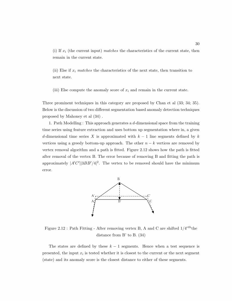
1. Path Modelling : This approach generates a d-dimensional space from the training

time series using feature extraction and uses bottom up segmentation where in, a given

d-dimensional time series X is approximated with k − 1 line segments defined by k

vertices using a greedy bottom-up approach. The other n − k vertices are removed by

vertex removal algorithm and a path is fitted. Figure 2.12 shows how the path is fitted

after removal of the vertex B. The error because of removing B and fitting the path is

approximately |A′C ′||3BB′/4|2. The vertex to be removed should have the minimum

error.

Figure 2.12 : Path Fitting - After removing vertex B, A and C are shifted 1/4rththe

distance from B’ to B. (34)

The states are defined by these k − 1 segments. Hence when a test sequence is

presented, the input xi is tested whether it is closest to the current or the next segment

(state) and its anomaly score is the closest distance to either of these segments.

31

2. Box modelling : This approach also generates a d-dimensional space from the

training time series using feature extraction and uses bottom up segmentation which

is an extension of the MBR (minimum bounding rectangle) approach to form boxes

which minimize the volume expansion. A sequence of n points in a feature space is first

approximated by a sequence of n − 1 boxes, each enclosing a pair of adjacent points.

Then pairs of adjacent boxes are merged by greedily selecting the pair that minimizes

the increase in volume after merging. This greedy split attempts to find a sequence of k

boxes with the least total volume. The boxes have the d-dimensional co-ordinates which

characterize the states. Hence the standard FSA is built on the states. To determine if a

test point xi belongs to a state, one has to check if it falls into the box corresponding to

the state. If the input does not fall into the current or next box then the anomaly score

of it is defined as the minimum distance to either of those boxes. The box modelling

approach has been extensively discussed in (33) by Chan et al. They use a 3D feature

space obtained from the data.

From the above illustrations, one could see that the variations in this category come

from (i) the methods used for constructing the FSA or the segmentation of time series,

(ii) the matching functions used to determine if an observation belongs to a certain state

and (iii) the anomaly score computation for each observation.

To construct an FSA, one or more training time series are partitioned into a series of

homogeneous segments, where each segment is termed as a state and the homegeneity

of a segment is characterized using a criterion function. There are different approaches

for segmenting a time series to obtain discrete states (66). Some traditional approaches

are : (i) Sliding window : Grow the segments from the time series until the error is

above a specified threshold, then start a new segment. (ii) Top-down : The entire time

series is recursively split until the desired number of segments is reached, or an error

threshold is reached (35). (iii) Bottom-up : The approaches by Mahoney et al (33; 34)

use this segmentation where they start with n2 (or n − 1) segments, the 2 most similar

adjacent segments are repeatedly joined until a stopping criterion is reached .

Salvador et al (35) propose a top-down approach using Gecko clustering to form the

initial groups. The rules which characterize these clusters are generated using RIPPER

(67). All the above techniques generate one FSA per time series. Box Modelling (33)

approach was extended to multiple time series by initially finding the boxes for one time

32

series and expanding the boxes to fit in the rest of the training time series.

The other variation in terms of matching function for a time series and anomaly

score assignment relate closely to how a state is characterized. The approaches described

above (33; 35; 34) use the following scheme. (1) If the state is enclosed, then check if xi

lies in that state, in which case its anomaly score is 0; If it does not lie in that state or

the next state, then it is either termed anomalous (35) or its anomaly score is computed

as the shortest distance to either of the states (current or next) (33). (2) If the state

is not enclosed, then the anomaly score of xi is its shortest distance to the current or

state.

The testing phase of above FSA is not robust to slight variations in the data which are

effected by the rigid boundaries of a state. Assume xl, . . . , xm and xm+2, . . . , xt match

a state sp , while xm+1 which is slightly outside sp and matches the next state sp+1.

According to the above FSA, once xm+1 falls into sp+1 the current state is modified to

sp+1and all the following observations, xm+2, . . . , xt are considered anomalous as they

do not match either the current state, sp+1 or the next state, sp+2, though they are

not anomalous. This issue is handled by Chan et al (33) by modifying step (b) of the

FSA, such that a transition to the next state (snext) occurs only if a specified number

of consecutive observations match the next state. Thus in our example, though xm+1

matches sp+1, xm+1, . . . xt do not match sp+1, hence xm+1 is considered anomalous and

the current state would still be sp.

Strengths and Weaknesses : The assumption of segmentation based techniques

is that the all the training time series can be partitioned into a group of homogeneous

segments. In cases where this cannot be done, segmentation based approaches might fail.

Also these techniques are highly inefficient as both the training phase of segmentation

and testing phase of checking each observation of each test time series with the FSA

are computationally intensive.

Segmentation based techniques build an FSA for the time series and compute anomaly

score for each of the observations in the time series. This helps in capturing all kinds

of anomalies : an anomalous observation in a time series, an anomalous subsequence in

a time series, an anomalous time series as a whole.

33

2.8 Discord Detection

The other important problem setting in anomaly detection as discussed in Section 2.2 is

discord detection. The general approach for finding the discord in a given test time

series Sq is as follows.

1. Divide Sq into t windows(subsequences), w1, w2, . . . wt, where t = |Sq|+ m− 1 by

sliding a window of size m, one step at a time.

2. Calculate the anomaly score for each window (A(wi)) by calculating its distance

from the other windows. Different distance/similarity measures like Euclidean,

Manhattan or Correlation can be chosen.

3. The window with maximum anomaly score is declared as the discord for the given

time-series.

As discussed in section 2.7.1, the windows can be obtained by sliding one or more

steps at a time, also called hop (h). If h < m, then the windows are overlapping. An

important issue to be considered in discord detection is : while comparing subsequences

with overlap, there is a chance that significant anomalies might be missed. This can be

seen in the following example. Consider the time series abcabcDDDabcababc , where

each symbol represents a real value and a sliding window of length 3. The significant

anomaly as can be seen is DDD. If the discord is defined as a subsequence farthest from

its nearest neighbour, then bab becomes our first discord as DDD has a close match

DDa within one step, which is also called a partial self-match, whereas bab does not

have a closer nearest neighbor. One way to avoid this problem, proposed by Keogh et

al (22), is to only consider non-self matches, i.e, a window is compared only with the

windows which do not overlap with it. Hence in the above example, DDD will not be

compared with cDD or DDa and will be considered as a discord.

A non-self match is formally defined as : “Given a time series T , containing a

subsequence C of length m beginning at position p and a matching subsequence M

beginning at q, we say that M is a non-self match to C at distance of Dist(M, C) if

|p − q| > m.” (22)

The issues with the window based approaches in discord detection are described

below. The techniques in this category mainly differ from each other in terms of how

34

they handle these issues.

1. Window size (m) : As discussed in Section 2.7.1, choosing the window size

is critical as it should be able to explicitly capture the anomaly. Most of the techniques

have a user defined window size parameter. Some of the techniques, as described in

(68; 69; 70) use the window size equal to the periodicity of the data which is computed

using the correlogram of the time series. A correlogram is known to be a graphical

representation of the auto correlation functions of the time series plotted with different

lags. The assumption is that if the time series is periodic then the correlation of the

original time series with a phased lagged version of it would give a maximum value, if

the phase lag is equal to its periodicity . Also the correlogram would have the same

periodicity as the process generating the original time series (69). Following the same

idea, Chuah and Fu (8) analyze ECG data using the window size as one heartbeat’s

length.

2. Anomaly score (A(sq)) : Calculation of anomaly score depends on which

similarity/distance measure is chosen and how the discord is defined. Palshikar et al

(71) define discord as the window which has maximum number of nearest neighbours

whose distance is greater than a user defined threshold. Their anomaly score is the

distance of a window to its nearest match including partial self-matches. For many

other techniques, discord is defined as the window which has the largest distance to its

nearest non-self match (72; 22; 39; 14). The anomaly score in this case is the distance

of a window to its nearest non-self match. Most of the discord detection techniques

consider the Euclidean distance measure. Das Gupta et al(40) discretize the time series

to obtain a binary representation and use simple matching of the windows, that is two

windows are identical if and only if r continuous bits match between the windows.

Cheng et al (17) proposed a graph based technique with the vertices being windows

and edge weights being the distances between the windows. The anomaly score, A(sq),

of a vertex is calculated as the connectivity of that vertex measured by a random walk on

the graph. An anomalous vertex would be highly different from others, so its similarity

(edge weight) with the other vertices in the graph would be small. Hence the probability

of visiting this vertex when performing a random walk is small. The authors generalized

35

this work to multivariate time series (17), where the same graph based priniciples are

applied in finding anomalous subsequences.

3. Efficiency : The general approach for window based anomaly detection

problem is O(n2) , where n is the length of the time-series. This is because, each possible

subsequence is considered (outer loop) and its distance to all the other subsequences

(inner loop) is calculated to find the nearest among them (71).

Most of the window based techniques for discord detection (72; 22; 39; 14) use an

approximation to the following heuristic ordering of the subsequences in order to make

the algorithm linearly scalable. For the outer loop : the subsequences are sorted by

descending order of the non-self distance to its nearest neighbor so that the true discord

is the first subsequence in the loop. For the inner loop: the subsequences are sorted

in ascending order of their distance to the current candidate. For such a heuristic,

since the first subsequence of the outer loop is the true discord, the largest nearest

neighbor distance (lmax) is found in the first pass of the inner loop. The subsequent

invocations of the inner loop will terminate in O(1) time as the distance of the outer loop

subsequence to its first inner loop subsequence is less than the existing threshold of the

maximum nearest neighbor distance (lmax) thus the outer loop subsequence cannot be

a discord, thus giving an O(n) algorithm. The approximation to this heuristic ordering

was obtained by specific data structures built on the SAX representation (22), wavelet

representation (44) of time series and these representations are also useful to improve

the efficiency further.

Instead of finding the most unusual discord, few approaches generalize it to finding

top-k discords (44). Also an important application of window based approaches is the

detection of shape anomalies (14). 2D shapes are converted to time series which are

shape invariant and the anomalies are detected using the same approaches mentioned

above.

2.9 Conclusions

This chapter summarizes the state of the art of anomaly detection techniques for uni-

variate time series. In Chapter 4, we investigate the behavior of these techniques on

36

publicly available data sets, each with different properties as discussed in Section 2.4.

Chapter 3

Subspace based transformation

for univariate timeseries

In the previous chapter, we discussed the problem of anomaly detection for time series

data and categorized the existing techniques based on their methodology and the way

they transform the data prior to anomaly detection. In this chapter we discuss a novel

transformation technique for univariate time series which uses concepts from the win-

dow based scheme discussed in section 2.7.1. We present the motivation behind this

transformation and the methodology in the following sections.

3.1 Motivation

In the discussion of window based techniques (section 2.7.1), we suggested that, once

the univariate test and training time series are divided into windows, any traditional

anomaly detection technique for multivariate data can be applied to these sets of win-

dows. The reason for this application is that if a normal univariate time series is

generated by a process, the windows of the normal time series also follow a generative

process in the multivariate space. Hence the set of fixed-length windows obtained from

a univariate time series can be considered as a multivariate time series. Univariate

anomalous time series follow a different process or do not follow any process; hence the

windows obtained from them need not follow the same process as the windows obtained

from normal time series.

37

38

We explain this with an example. Consider the normal time series in Figure 3.1(a).

The first few windows of it are shown in Figure 3.1(c) (obtained with parameters: win-

dow length n = 250 and number of steps (hop) h = 10). We consider each of the time

instance of a window as a variable, i.e., if the window length is n then the multivariate

time series has n variables. In Figure 3.2 we show the time series corresponding to a

sample of these variables. Figure 3.2(a) shows the time series corresponding to time

instances (variables) 50 , 150 and 200 of the windows obtained from normal time series

in Figure 3.1(a). We will refer to these variables as normal variables. Similarly Fig-

ure 3.2(b) shows the time series corresponding to same time instances of the windows

obtained from the anomalous time series in Figure 3.1(b). As can be seen, the time

series of normal variables follow a periodic pattern, while the time series of anomalous

variables does not follow the periodic pattern. Hence these windows from univariate

time series can be considered as multivariate time series as they follow a specific process

in the multivariate space.

With this motivation we proceed to present a brief overview of multivariate time

series and anomaly detection techniques in this domain in section 3.2.

3.2 Detecting Anomalies in Multivariate Time Series

Data collected in many application domains consists of multivariate time series. For

example, a single aircraft generates different univariate time series, which are considered

as a single multivariate time series. Each of these univariate time series correspond to

data coming from a single sensor or a switch on the aircraft (73). Similarly the daily

network log stored for network intrusion detection depicts a multivariate time series,

where each variable measures certain aspects of the time series (74).

Anomaly detection for multivariate time series data is distinct from traditional

anomaly detection for multivariate data as well as anomaly detection for univariate

time series data. This is because the anomaly detection techniques for multivariate

data analyse only the multivariate aspect of the data, while the techniques for univari-

ate time series data analyse the sequence aspect of each variable independently. Often,

the anomaly in a multivariate time series can be detected only by analyzing the sequence

of all (or a subset of) variables.

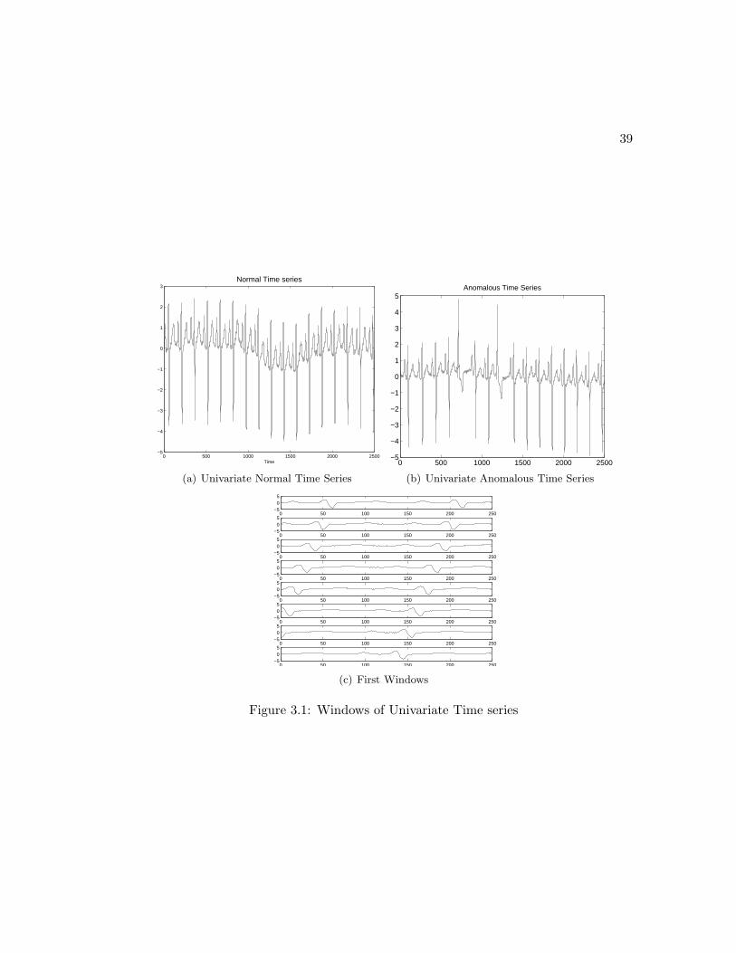
39

0 500 1000 1500 2000 2500−5

−4

−3

−2

−1

0

1

2

3

Time

Normal Time series

(a) Univariate Normal Time Series

0 500 1000 1500 2000 2500−5

−4

−3

−2

−1

0

1

2

3

4

5Anomalous Time Series

(b) Univariate Anomalous Time Series

0 50 100 150 200 250−5

05

0 50 100 150 200 250−5

05

0 50 100 150 200 250−5

05

0 50 100 150 200 250−5

05

0 50 100 150 200 250−5

05

0 50 100 150 200 250−5

05

0 50 100 150 200 250−5

05

0 50 100 150 200 250−5

05

(c) First Windows

Figure 3.1: Windows of Univariate Time series

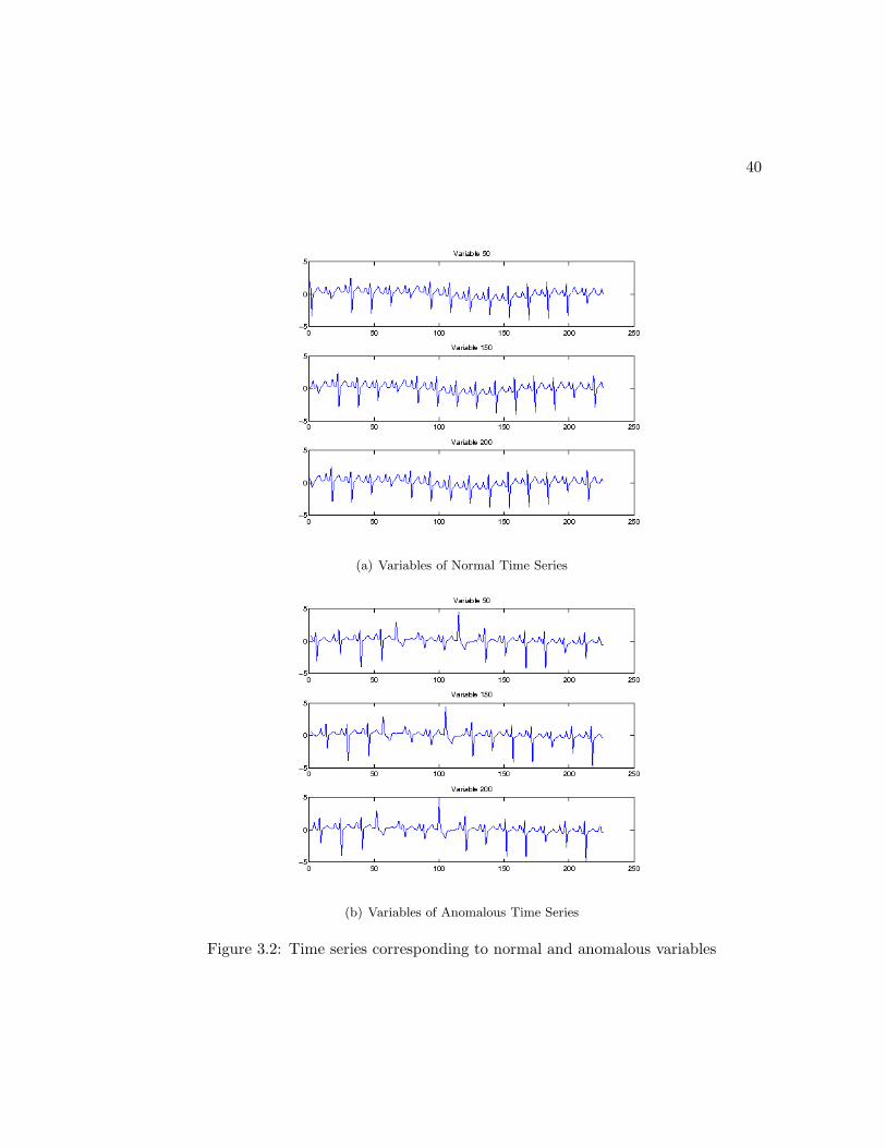
40

(a) Variables of Normal Time Series

(b) Variables of Anomalous Time Series

Figure 3.2: Time series corresponding to normal and anomalous variables

41

A real life instance of anomalies in multivariate time series data can be found in

aviation safety domain (73). During the course of the flight of an aircraft, multiple

sensors measure different aspects of the flight, thereby generating a multivariate time

series. An fault or accident during the flight of the aircraft can be detected by finding

anomalies in the multivariate time series data. To detect such anomalies in multivariate

sequences, multivariate aspect as well as the sequence aspect needs to be simultaneously

modeled.

A multivariate anomaly detection technique proposed by Chandola (75), is a window

based technique which accounts for both the multivariate and sequence aspects of the

data while detecting anomalies. The key underlying idea is to reduce a multivariate time

series into a univariate time series by exploring the change in the correlation structure of

the time series, using subspace monitoring. We discuss subspace monitoring in section

3.2.1 and the anomaly detection technique for multivariate time series using subspace

monitoring, WINSS in section 3.2.2.

3.2.1 Subspace Monitoring for Multivariate Time Series

Subspace monitoring for damage detection and other related areas falls under the broad

purview of statistical process control (76; 77). Jordan et al (78) proposed the original

concept of comparing two subspaces using the angles between their principal compo-

nents, which was later explained as canonical correlation by Hotelling (79). Chandola

et al (75) provide a detailed discussion of the angle between subspaces using principal

angles.

Comparison of multivariate time series often use subspace based analysis, so as to

compare their generative models such as vector AR models (80), ARMA models (81),

and linear dynamical systems (76). It has been shown that the modes and modal shapes

of vibrating structures (76) coincide with their system eigenstructure. Any change in

this structure can be computed using covariance driven identification methods which

use the change in subspaces.

The anomaly detection technique proposed by Chandola et al (75) measures the

change between two subspaces, SA and SB , which is defined as the following (77):

Change in subspace when SA changes to subspace SB is equal to the maximum distance

between an arbitrary unit vector x in SB and the subspace SA. This change δAB is given

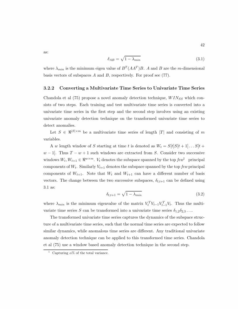
42

as:

δAB =√

1 − λmin (3.1)

where λmin is the minimum eigen value of BT (AAT )B. A and B are the m-dimensional

basis vectors of subspaces A and B, respectively. For proof see (77).

3.2.2 Converting a Multivariate Time Series to Univariate Time Series

Chandola et al (75) propose a novel anomaly detection technique, WINSS which con-

sists of two steps. Each training and test multivariate time series is converted into a

univariate time series in the first step and the second step involves using an existing

univariate anomaly detection technique on the transformed univariate time series to

detect anomalies.

Let S ∈ ℜ|S|×m be a multivariate time series of length |T | and consisting of m

variables.

A w length window of S starting at time t is denoted as Wt = S[t]S[t + 1] . . . S[t +

w − 1]. Thus T − w + 1 such windows are extracted from S. Consider two successive

windows Wt,Wt+1 ∈ ℜw×m. Vt denotes the subspace spanned by the top few1 principal

components of Wt. Similarly Vt+1 denotes the subspace spanned by the top few principal

components of Wt+1. Note that Wt and Wt+1 can have a different number of basis

vectors. The change between the two successive subspaces, δt,t+1 can be defined using

3.1 as:

δt,t+1 =√

1 − λmin (3.2)

where λmin is the minimum eigenvalue of the matrix V Tt Vt−1V

Tt−1Vt. Thus the multi-

variate time series S can be transformed into a univariate time series δ1,2δ2,3 . . ..

The transformed univariate time series captures the dynamics of the subspace struc-

ture of a multivariate time series, such that the normal time series are expected to follow

similar dynamics, while anomalous time series are different. Any traditional univariate

anomaly detection technique can be applied to this transformed time series. Chandola

et al (75) use a window based anomaly detection technique in the second step.

1 Capturing α% of the total variance.

43

3.3 Transformation

Section 3.2.2 describes how the anomaly in the multivariate space can be captured using

the subspace based analysis by exploring the correlation structure of the multivariate

time series. With this motivation, we proceed further to apply the subspace analysis

to the windows obtained from univariate time series which can be considered as multi-

variate time series. The process of this subspace based transformation is : converting a

univariate time series to a multivariate time series and back to another univariate time

series.

3.3.1 Methodology

For a given univariate time series T of length N , T = t1t2 . . . tN , overlapping win-

dows of length n are created. Let wi be the ith window which can be represented as

titi+1 . . . ti+n−1. These windows are stacked and are considered as multivariate time

series, W , represented as :

w1

w2

...

wN−n+1

=

t1 t2 . . . tn

t2 t3 . . . tn+1

......

......

tN−n+1 tN−n+2 . . . tN

Each time instance of a window is considered as a variable, so the columns correspond

to time series of different variables. The time series corresponding to kth variable is

tktk+1tk+2 . . . and the length of the multivariate time series is the number of windows

extracted. As discussed in section 2.7.1, the windows from a univariate time series can

be obtained by sliding one or more steps at a time, also called hop (h). In the above

case we considered h = 1. If h < n, the windows are overlapping. For any general hop

h, the time series corresponding to kth variable is tktk+htk+2h . . ..

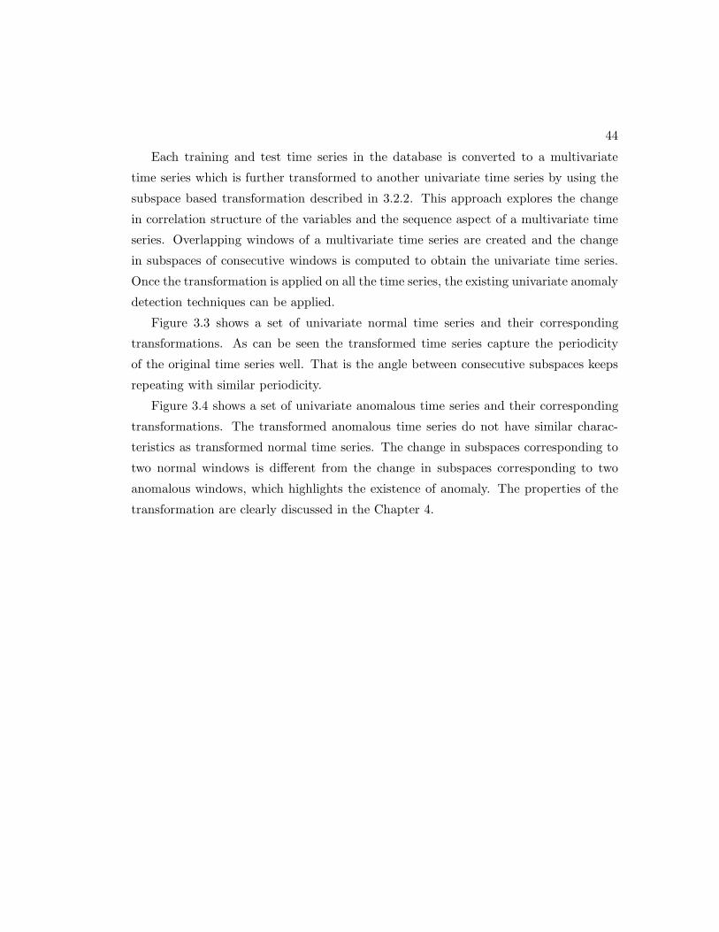
44

Each training and test time series in the database is converted to a multivariate

time series which is further transformed to another univariate time series by using the

subspace based transformation described in 3.2.2. This approach explores the change

in correlation structure of the variables and the sequence aspect of a multivariate time

series. Overlapping windows of a multivariate time series are created and the change

in subspaces of consecutive windows is computed to obtain the univariate time series.

Once the transformation is applied on all the time series, the existing univariate anomaly

detection techniques can be applied.

Figure 3.3 shows a set of univariate normal time series and their corresponding

transformations. As can be seen the transformed time series capture the periodicity

of the original time series well. That is the angle between consecutive subspaces keeps

repeating with similar periodicity.

Figure 3.4 shows a set of univariate anomalous time series and their corresponding

transformations. The transformed anomalous time series do not have similar charac-

teristics as transformed normal time series. The change in subspaces corresponding to

two normal windows is different from the change in subspaces corresponding to two

anomalous windows, which highlights the existence of anomaly. The properties of the

transformation are clearly discussed in the Chapter 4.

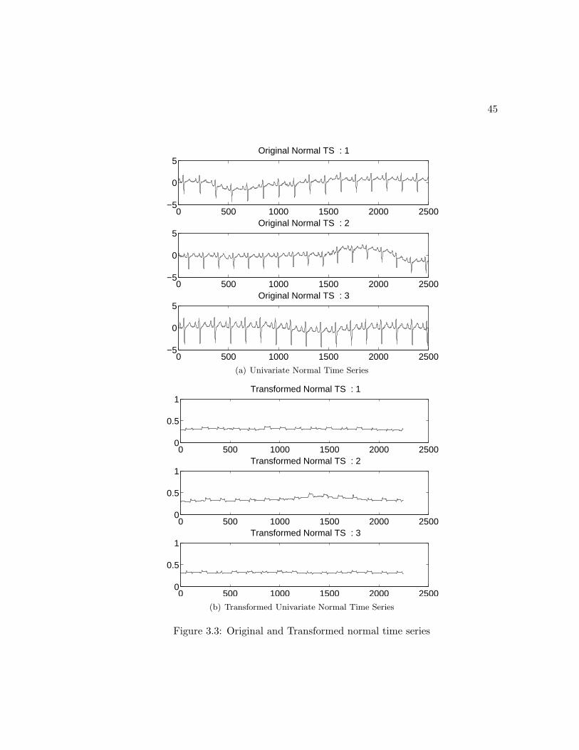
45

0 500 1000 1500 2000 2500−5

0

5Original Normal TS : 1

0 500 1000 1500 2000 2500−5

0


0 500 1000 1500 2000 2500−5

0


(a) Univariate Normal Time Series

0 500 1000 1500 2000 25000

0.5

1Transformed Normal TS : 1

0 500 1000 1500 2000 25000

0.5


0 500 1000 1500 2000 25000

0.5


(b) Transformed Univariate Normal Time Series

Figure 3.3: Original and Transformed normal time series

46

0 500 1000 1500 2000 2500−5

0

5Original Anomalous TS : 1

0 500 1000 1500 2000 2500−5

0


0 500 1000 1500 2000 2500−5

0


(a) Univariate Anomalous Time Series

0 500 1000 1500 2000 25000

0.5

1Transformed Anomalous TS : 1

0 500 1000 1500 2000 25000

0.5


0 500 1000 1500 2000 25000

0.5


(b) Transformed Univariate Anomalous Time Series

Figure 3.4: Original and Transformed Anomalous time series

Chapter 4

Experiments and Discussion

In this chapter we investigate the behavior of the anomaly detection techniques dis-

cussed in Chapter 2 and also the transformation technique discussed in Chapter 3. The

experimental evaluation of the existing anomaly detection techniques on various publicly

available datasets has been thoroughly discussed by Chandola et al (26).

This chapter provides results and discussions from two different experiments. One

is a brief discussion on the strengths and weaknesses of the existing anomaly detection

techniques on the original time series and their discretized versions. The other one,

which is the focus of the thesis, is on the comparison of existing anomaly detection

techniques (see chapter 2) on a variety of publicly available datasets, with the same

techniques after applying the subspace based transformation (see chapter 3) on these

datasets.

We provide a thorough experimental framework for understanding these techniques

on the transformed time series obtained from the subspace based transformation. The

transformation essentially converts a given univariate time series to a multivariate time

series and back to another univariate time series. We provide the experimental evalua-

tion using data sets with different properties to understand the types of time series on

which the transformation works best.

The rest of the chapter is organized as follows. Section 4.1 briefly describes the

different anomaly detection techniques for time series data. Section 4.2 describes the

different kinds of data sets used for this experimental evaluation. Section 4.3 summarizes

our experimental results of using different anomaly detection techniques on the publicly

47

48

available data sets. Section 4.4 shows the results of using different anomaly detection

technniques on the transformed time series.

4.1 Anomaly Detection Techniques

The following techniques were investigated by Chandola et al (26).

• Proximity Based Techniques These techniques make use of a proximity mea-

sure defined for every pair of time series. We evaluate a nearest neighbor based

technique, called KNNC (k-nearest neighbor for continuous time series) (82),

that utilizes this proximity measure. KNNC assigns an anomaly score to a test

time series, as equal to its distance to its kth nearest neighbor in the training

database, X.

A discrete version of KNNC called KNND is also evaluated (where ‘D’ stands

for Discrete), where a continuous time series is initially discretized into a sequence

of symbols using symbolic approximation (SAX) technique (22).

For KNNC, we evaluate three distance measures, viz., Euclidean Distance, Dy-

namic Time Warp (DTW ) (83), and Cross Correlation (84).

• Window Based Techniques These techniques extract fixed length (w) windows

from a test time series, and assign an anomaly score to each window. The per-

window scores are then, aggregated to obtain the anomaly score for the test time

series. The score assignment to a window and the score aggregation can be done

in different ways.

We denote the window based techniques for continuous time series as WINC.

The experimented version of WINC assigns an anomaly score to each window

of a test time series equal to the Euclidean distance between the window and

its kth nearest neighbor in the set of windows extracted from the training time

series. The anomaly score for the test time series is equal to the average score

of all its windows. WINC estimates the density of w-dimensional windows using

the windows extracted from the training time series and then determine if the

windows extracted from a test time series lie in the dense regions or not.

49

The discrete version of this called WIND is also evaluated. We evaluated two

variants of WIND: WIND and tSTIDE. WIND is similar to WINC with

the only difference being that the score for each window from a test sequence is a

likelihood score (inverse of anomaly score), and is equal to the similarity between

the window and its kth nearest neighbor in the set of windows extracted from

the training sequences. For tSTIDE (proposed by Forrest et al (85) for symbolic

sequences), the likelihood score for each window is equal to, the number of times

the window occurs in the set of training windows (windows extracted from the

training sequences), divided by the total number of training windows.

• Prediction Based Techniques These techniques learn a predictive model from

the training time series. Testing involves forecasting the next observation in a test

time series, using the predictive model and the test time series observed so far, and

comparing the forecasted observation with the actual observation to determine if

an anomaly has occurred.

We evaluate three predictive techniques: AR (using Auto Regressive models (52)),

SV R (using Support Vector Regression (86)), and FSAz (using Finite State Au-

tomata based technique for symbolic sequences (87)). For AR and SV R, the

anomaly score for each observation in a test time series is equal to the difference

between the forecasted value and the actual observation. The anomaly score of the

test time series is equal to the average anomaly scores for all of its observations.

For FSAz, a likelihood score is obtained for each symbol in the discretized test

sequence which is equal to the conditional probability of observing the symbol in

the training sequences, given the previous few symbols. The anomaly score for the

discretized test sequence is equal to the inverse of the average likelihood scores for

all of its symbols.

4.2 Data Sets Used

To evaluate the performance of each algorithm, 18 publicly available data sets are used.

Table 4.1 summarizes the different data sets for the cross-domain experimental evalua-

tion. These datasets are grouped into different categories, each with distinct character-

istics as discussed in Section 2.4. For the periodic time series, the last column denotes

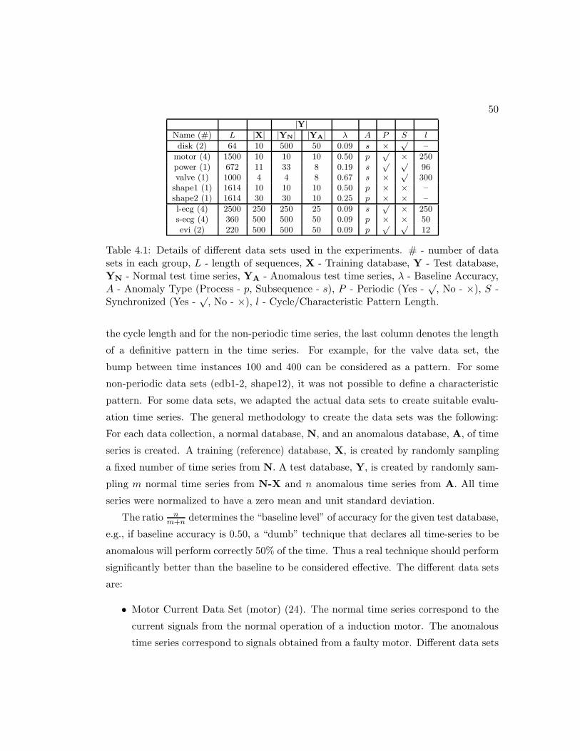
50

|Y|Name (#) L |X| |YN| |YA| λ A P S l

disk (2) 64 10 500 50 0.09 s × √–

motor (4) 1500 10 10 10 0.50 p√ × 250

power (1) 672 11 33 8 0.19 s√ √

96valve (1) 1000 4 4 8 0.67 s × √

300shape1 (1) 1614 10 10 10 0.50 p × × –shape2 (1) 1614 30 30 10 0.25 p × × –

l-ecg (4) 2500 250 250 25 0.09 s√ × 250

s-ecg (4) 360 500 500 50 0.09 p × × 50evi (2) 220 500 500 50 0.09 p

√ √12

Table 4.1: Details of different data sets used in the experiments. # - number of datasets in each group, L - length of sequences, X - Training database, Y - Test database,YN - Normal test time series, YA - Anomalous test time series, λ - Baseline Accuracy,A - Anomaly Type (Process - p, Subsequence - s), P - Periodic (Yes -

√, No - ×), S -

Synchronized (Yes -√

, No - ×), l - Cycle/Characteristic Pattern Length.

the cycle length and for the non-periodic time series, the last column denotes the length

of a definitive pattern in the time series. For example, for the valve data set, the

bump between time instances 100 and 400 can be considered as a pattern. For some

non-periodic data sets (edb1-2, shape12), it was not possible to define a characteristic

pattern. For some data sets, we adapted the actual data sets to create suitable evalu-

ation time series. The general methodology to create the data sets was the following:

For each data collection, a normal database, N, and an anomalous database, A, of time

series is created. A training (reference) database, X, is created by randomly sampling

a fixed number of time series from N. A test database, Y, is created by randomly sam-

pling m normal time series from N-X and n anomalous time series from A. All time

series were normalized to have a zero mean and unit standard deviation.

The ratio nm+n

determines the “baseline level” of accuracy for the given test database,

e.g., if baseline accuracy is 0.50, a “dumb” technique that declares all time-series to be

anomalous will perform correctly 50% of the time. Thus a real technique should perform

significantly better than the baseline to be considered effective. The different data sets

are:

• Motor Current Data Set (motor) (24). The normal time series correspond to the

current signals from the normal operation of a induction motor. The anomalous

time series correspond to signals obtained from a faulty motor. Different data sets

51

(motor1 motor4) correspond to different kinds of faults in the motor.

• Power Usage Data (power) (24). The normal time series correspond to weekly

time series of power consumption at a research facility in 1997 for weeks with no

holidays during the weekdays. The anomalous time series correspond to power

consumption during weeks with a holiday during the week.

• NASA Valve Data (valve) (24). The normal time series consists of TEK solenoid

current measurements recorded during the normal operation of a Marrotta series

valves located on a space shuttle. The anomalous time series correspond to the

faulty operation of the valve.

• Shape Data (shape1 and shape2) (24). The normal time series correspond to one

or more shapes, while the anomalous time series correspond to other shapes. For

the shape1 database, the normal time series correspond to a pencil shape, while

the anomalous time series correspond to other similar shapes (e.g., fork). For the

shape2 database, the normal time series correspond to shapes of cups, glasses,

and crosses, while the anomalous time series correspond to distinctly dissimilar

shapes.

• Electrocardiogram Data (l-ecg and s-ecg) (25). Each data set corresponds to an

ECG recording for one subject suffering with a particular heart condition. The

ECG recording is segmented into short time series of equal lengths. Each short

time series is added to the normal database if it does not contain any annotations

of a heart condition2 , and is added to the anomalous database if it contains one

or more annotations indicating a heart condition. The l-ecg databases contain 10

second long time series. Four such databases (l-ecg1l-ecg4) were constructed from

BIDMC Congestive Heart Failure Database and Long-Term ST Database. The

s-ecg databases contain 1 second long time series. Four such databases (s-ecg1s-

ecg4) were constructed from European ST-T Database and MIT-BIH Arrhythmia

Database.

• EVI Data (evi1 and evi2) (88). Enhanced Vegetation Index essentially serves as

a measure of the amount and “greenness” of vegetation at a particular location.

Each land location has a time series of length T which corresponds to T monthly

52

observations at that location. A normal time series corresponds to periodic cycles

of vegetation with high values in summer and low values in winter. An anomalous

time series corresponds to places where there was land cover change because of a

natural calamity or forest fires. This dataset is used only for the experiments on

the transformation technique.

• Disk Defect Data Set (disk) (89). The normal time series corresponds to blade

tip clearance measurements obtained from a simulated aircraft engine disk and the

anomalous time series correspond to the measurements obtained from a disk with

a crack. Different data sets (disk1 – disk3) correspond to different speeds at which

the disk is rotating. This dataset has not been used for transformation evaluation

but used for the generic comparison of anomaly detection techniques.

4.3 Comparison of Anomaly Detection Techniques

In this section we first provide the results for the experimental evaluation of anomaly

detection techniques discussed by Chandola et al (26). For each technique, we use the

parameters that result in the best average performance over all datasets. The accuracy

results (or precision on normal class) of the techniques using these best parameter

settings are reported in Table 4.3. The results reveal several interesting insights into

the performance of the different techniques. At a high level, our results indicate that

none of the techniques are superior to others across all data sets, but have certain

characteristics that make them effective for certain types of data sets, and ineffective

for certain others. Here we summarize some high level conclusions:

• Techniques that operate on the continuous time series are generally superior to tech-

niques that operate on discrete sequences. Moreover, techniques for continuous time

series are more robust to parameter choices such as distance measure (KNNC vs.

KNND) or window length (WINC vs. WIND).

• Overall, kernel and window based techniques, which are model independent, tend to

outperform predictive and segmentation based techniques, that try to build a model

for the time series data. This seems to indicate that building a predictive model for

time series data is challenging.

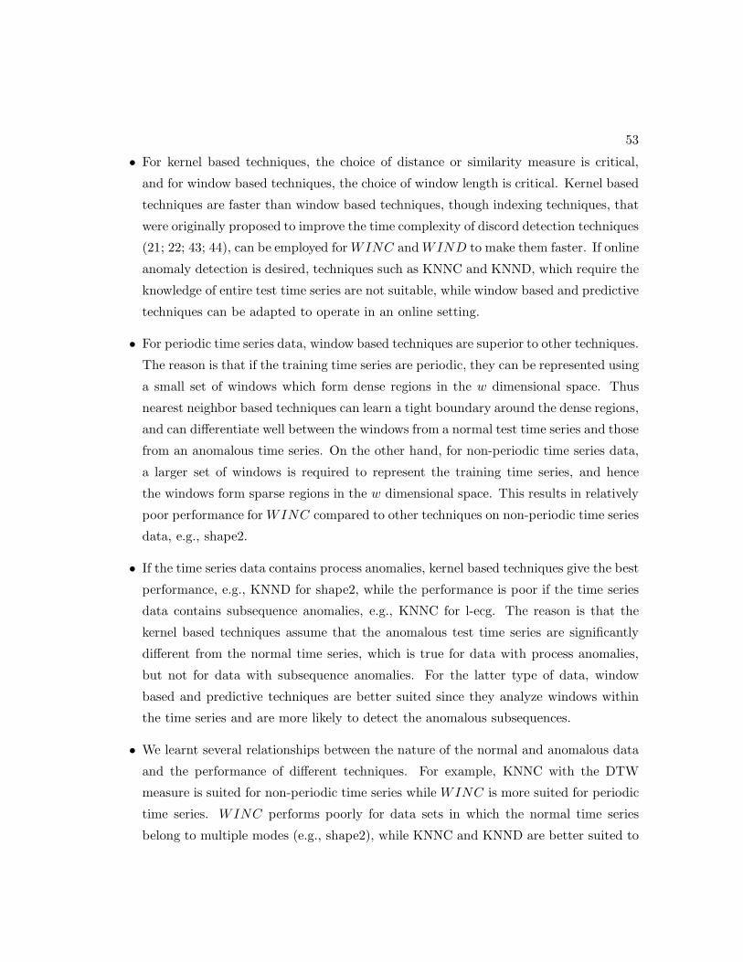
53

• For kernel based techniques, the choice of distance or similarity measure is critical,

and for window based techniques, the choice of window length is critical. Kernel based

techniques are faster than window based techniques, though indexing techniques, that

were originally proposed to improve the time complexity of discord detection techniques

(21; 22; 43; 44), can be employed for WINC and WIND to make them faster. If online

anomaly detection is desired, techniques such as KNNC and KNND, which require the

knowledge of entire test time series are not suitable, while window based and predictive

techniques can be adapted to operate in an online setting.

• For periodic time series data, window based techniques are superior to other techniques.

The reason is that if the training time series are periodic, they can be represented using

a small set of windows which form dense regions in the w dimensional space. Thus

nearest neighbor based techniques can learn a tight boundary around the dense regions,

and can differentiate well between the windows from a normal test time series and those

from an anomalous time series. On the other hand, for non-periodic time series data,

a larger set of windows is required to represent the training time series, and hence

the windows form sparse regions in the w dimensional space. This results in relatively

poor performance for WINC compared to other techniques on non-periodic time series

data, e.g., shape2.

• If the time series data contains process anomalies, kernel based techniques give the best

performance, e.g., KNND for shape2, while the performance is poor if the time series

data contains subsequence anomalies, e.g., KNNC for l-ecg. The reason is that the

kernel based techniques assume that the anomalous test time series are significantly

different from the normal time series, which is true for data with process anomalies,

but not for data with subsequence anomalies. For the latter type of data, window

based and predictive techniques are better suited since they analyze windows within

the time series and are more likely to detect the anomalous subsequences.

• We learnt several relationships between the nature of the normal and anomalous data

and the performance of different techniques. For example, KNNC with the DTW

measure is suited for non-periodic time series while WINC is more suited for periodic

time series. WINC performs poorly for data sets in which the normal time series

belong to multiple modes (e.g., shape2), while KNNC and KNND are better suited to

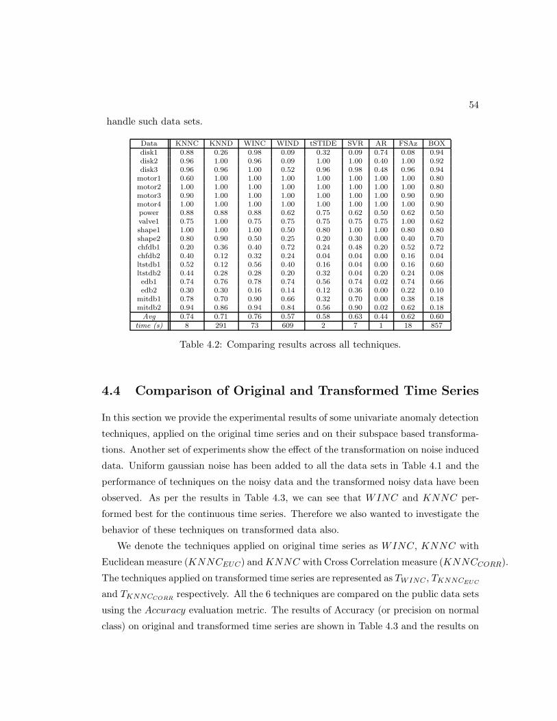
54

handle such data sets.

Data KNNC KNND WINC WIND tSTIDE SVR AR FSAz BOXdisk1 0.88 0.26 0.98 0.09 0.32 0.09 0.74 0.08 0.94disk2 0.96 1.00 0.96 0.09 1.00 1.00 0.40 1.00 0.92disk3 0.96 0.96 1.00 0.52 0.96 0.98 0.48 0.96 0.94

motor1 0.60 1.00 1.00 1.00 1.00 1.00 1.00 1.00 0.80motor2 1.00 1.00 1.00 1.00 1.00 1.00 1.00 1.00 0.80motor3 0.90 1.00 1.00 1.00 1.00 1.00 1.00 0.90 0.90motor4 1.00 1.00 1.00 1.00 1.00 1.00 1.00 1.00 0.90power 0.88 0.88 0.88 0.62 0.75 0.62 0.50 0.62 0.50valve1 0.75 1.00 0.75 0.75 0.75 0.75 0.75 1.00 0.62shape1 1.00 1.00 1.00 0.50 0.80 1.00 1.00 0.80 0.80shape2 0.80 0.90 0.50 0.25 0.20 0.30 0.00 0.40 0.70chfdb1 0.20 0.36 0.40 0.72 0.24 0.48 0.20 0.52 0.72chfdb2 0.40 0.12 0.32 0.24 0.04 0.04 0.00 0.16 0.04ltstdb1 0.52 0.12 0.56 0.40 0.16 0.04 0.00 0.16 0.60ltstdb2 0.44 0.28 0.28 0.20 0.32 0.04 0.20 0.24 0.08edb1 0.74 0.76 0.78 0.74 0.56 0.74 0.02 0.74 0.66edb2 0.30 0.30 0.16 0.14 0.12 0.36 0.00 0.22 0.10

mitdb1 0.78 0.70 0.90 0.66 0.32 0.70 0.00 0.38 0.18mitdb2 0.94 0.86 0.94 0.84 0.56 0.90 0.02 0.62 0.18Avg 0.74 0.71 0.76 0.57 0.58 0.63 0.44 0.62 0.60

time (s) 8 291 73 609 2 7 1 18 857

Table 4.2: Comparing results across all techniques.

4.4 Comparison of Original and Transformed Time Series

In this section we provide the experimental results of some univariate anomaly detection

techniques, applied on the original time series and on their subspace based transforma-

tions. Another set of experiments show the effect of the transformation on noise induced

data. Uniform gaussian noise has been added to all the data sets in Table 4.1 and the

performance of techniques on the noisy data and the transformed noisy data have been

observed. As per the results in Table 4.3, we can see that WINC and KNNC per-

formed best for the continuous time series. Therefore we also wanted to investigate the

behavior of these techniques on transformed data also.

We denote the techniques applied on original time series as WINC, KNNC with

Euclidean measure (KNNCEUC) and KNNC with Cross Correlation measure (KNNCCORR).

The techniques applied on transformed time series are represented as TWINC , TKNNCEUC

and TKNNCCORRrespectively. All the 6 techniques are compared on the public data sets

using the Accuracy evaluation metric. The results of Accuracy (or precision on normal

class) on original and transformed time series are shown in Table 4.3 and the results on

55

their noisy counterparts are shown in 4.4. These tables show the best accuracies of the

techniques on all data sets over different parameter settings.

Figure 4.1 shows the average accuracies of the techniques over the periodic and non-

periodic datasets separately and Figure 4.2 the same for the noise induced datasets.

These tables show the best accuracies of the techniques on all data sets over different

parameter settings.

For all the techniques, we experimented with different parameter settings listed

below :

• Window size (w1) to extract windows to form the multivariate time series :

( l2 , l , 2l), where l is the Cycle/Characteristic Pattern Length in the time series.

• Window size (w2) to extract windows from the multivariate time series for the

transformation : (4 , 6 , 8 , 10)

• The percentage of total variance captured by the subspace, α : (0.75 − 0.95)

The effect of these parameters settings and the characteristics of the data on the

transformation are discussed in the section 4.5.

DataSet WINC TWINC KNNCEUC TKNNCEUCKNNCCORR TKNNCCORR

1. motor1 1.00 1.00 1.00 1.00 1.00 1.002. motor2 1.00 1.00 1.00 1.00 1.00 1.003. motor3 1.00 1.00 1.00 1.00 0.90 1.004. motor4 1.00 1.00 1.00 1.00 1.00 1.005. power 0.88 0.75 0.88 0.88 0.88 0.886. chfdb1 0.72 0.64 0.12 0.76 0.20 0.687. chfdb2 0.32 0.44 0.16 0.52 0.40 0.408. ltstdb1 0.80 0.80 0.12 0.80 0.52 0.769. ltstdb2 0.28 0.32 0.24 0.44 0.44 0.3210. evi1 0.98 0.75 1.00 0.98 0.30 0.3611. evi2 0.88 0.83 1.00 0.96 0.10 0.3912. valve1 0.75 0.75 0.75 1.00 0.75 0.7513. edb1 0.78 0.50 0.68 0.52 0.74 0.4014. edb2 0.16 0.22 0.22 0.30 0.38 0.2815. mitdb1 0.84 0.64 0.70 0.60 0.80 0.5016. mitdb2 0.94 0.70 0.90 0.70 0.94 0.6017. shapes1 1.00 1.00 0.90 1.00 1.00 1.0018. shapes2 0.50 0.20 0.90 1.00 0.80 0.80

Avg 0.74 0.64 0.65 0.78 0.63 0.65Time(s) 74 80 6 15 9 17

Table 4.3: Accuracy Results

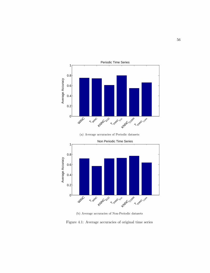
56

0

0.2

0.4

0.6

0.8

1

WIN

CT W

INC

KNNC EUC

T KNNC EUC

KNNC CORR

T KNNC CORR

Ave

rage

Acc

urac

yPeriodic Time Series

(a) Average accuracies of Periodic datasets

0

0.2

0.4

0.6

0.8

1

WIN

CT W

INC

KNNC EUC

T KNNC EUC

KNNC CORR

T KNNC CORR

Ave

rage

Acc

urac

y

Non Periodic Time Series

(b) Average accuracies of Non-Periodic datasets

Figure 4.1: Average accuracies of original time series

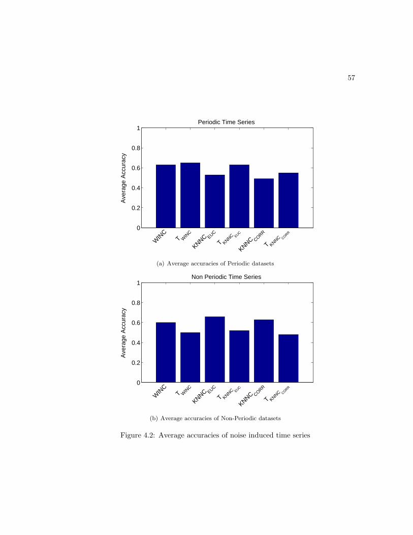
57

0

0.2

0.4

0.6

0.8

1

WIN

CT W

INC

KNNC EUC

T KNNC EUC

KNNC CORR

T KNNC CORR

Ave

rage

Acc

urac

yPeriodic Time Series

(a) Average accuracies of Periodic datasets

0

0.2

0.4

0.6

0.8

1

WIN

CT W

INC

KNNC EUC

T KNNC EUC

KNNC CORR

T KNNC CORR

Ave

rage

Acc

urac

y

Non Periodic Time Series

(b) Average accuracies of Non-Periodic datasets

Figure 4.2: Average accuracies of noise induced time series

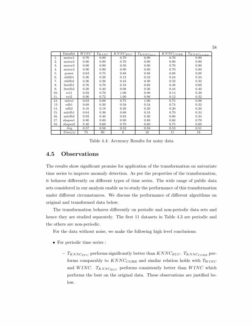
58

DataSet WINC TWINC KNNCEUC TKNNCEUCKNNCCORR TKNNCCORR

1. motor1 0.70 0.90 0.70 0.90 0.70 0.902. motor2 0.90 0.90 0.70 0.90 0.90 0.903. motor3 0.80 0.90 0.50 0.90 0.70 0.904. motor4 0.90 0.90 0.90 0.80 0.70 0.805. power 0.63 0.75 0.88 0.88 0.88 0.886. chfdb1 0.36 0.28 0.12 0.32 0.24 0.247. chfdb2 0.36 0.36 0.24 0.30 0.32 0.328. ltstdb1 0.76 0.70 0.16 0.68 0.48 0.609. ltstdb2 0.20 0.40 0.08 0.36 0.44 0.4010. evi1 0.92 0.70 1.00 0.98 0.14 0.3811. evi2 0.90 0.72 1.00 0.96 0.12 0.3212. valve1 0.63 0.88 0.75 1.00 0.75 0.8813 edb1 0.68 0.30 0.58 0.34 0.74 0.3214. edb2 0.16 0.18 0.20 0.20 0.20 0.2015. mitdb1 0.64 0.36 0.68 0.34 0.70 0.3416. mitdb2 0.92 0.40 0.82 0.36 0.80 0.3417. shapes1 0.80 0.80 0.90 0.80 0.60 0.7018. shapes2 0.40 0.60 0.70 0.60 0.75 0.60

Avg 0.57 0.56 0.52 0.58 0.53 0.51Time(s) 73 80 6 16 11 18

Table 4.4: Accuracy Results for noisy data

4.5 Observations

The results show significant promise for application of the transformation on univariate

time series to improve anomaly detection. As per the properties of the transformation,

it behaves differently on different types of time series. The wide range of public data

sets considered in our analysis enable us to study the performance of this transformation

under different circumstances. We discuss the performance of different algorithms on

original and transformed data below.

The transformation behaves differently on periodic and non-periodic data sets and

hence they are studied separately. The first 11 datasets in Table 4.3 are periodic and

the others are non-periodic.

For the data without noise, we make the following high level conclusions.

• For periodic time series :

– TKNNCEUCperforms significantly better than KNNCEUC . TKNNCCORR

per-

forms comparably to KNNCCORR and similar relation holds with TWINC

and WINC. TKNNCEUCperforms consistently better than WINC which

performs the best on the original data. These observations are justified be-

low.

59

– For window based technique, WINC, the optimal size of the window depends

on the length of anomalous region in the anomalous time series. Anomalies in

periodic time series can vary such as irregular periods, anomalous values etc.

Hence if the parameters such as window length, hop and nearest neighbors

are set appropriately, WINC performs well.

– The phase-misalignments and non-linear alignments, which are some common

challenges of periodic time series data, restrict the usage of different proximity

measures for the proximity based techniques. Thus KNNCEUC performs

well only when the time series are synchronous, while KNNCCORR works

moderately well given that it tries to align phases and compute similarity.

– After the transformation, the normal periodic time series become periodic or

constant valued time series. Since the normal periodic time series would not

have varying periods or anomalous values, the change in angle between con-

secutive subspaces of windows nearly remains constant or varies with some

periodicity. The transformed anomalous time series highlight the existence

of anomaly. Since the change in angle between consecutive subspaces is gov-

erned by the maximum distance between an arbitrary unit vector in one

subspace and the other suspace, even a small change in one of the subspaces

will change the angle significantly. This property of the transformation en-

ables it to highlight the existence of the anomaly in the time series. Thus the

transformed anomalous time series is signigicantly different from the normal

time series. In figure 3.4, the spikes in the transformed anomalous time se-

ries correspond to the entry and exit of the anomalous portion of the original

time series in the windows of the multivariate time series.

– The above aspects of the transformed time series make them more suited for

the proximity based scheme with Euclidean distance measure (TKNNCEUC)

as it performs consistently the best when (i) the normal time series are syn-

chronous (the constant valued time series) while the anomalous portions are

highlighted in the anomalous time series, or (ii) when the normal time series

are periodic and the portions of anomalous time series are highly different

from the normal ones.

60

– TWINC is not always better than WINC because the performance of a win-

dow based scheme is highly dependent on the appropriate parameter sett-

tings.

– Performance of TKNNCCORRis typically next to TKNNCEUC

in most cases.

This is because for the anomalous time series, the correlation measure finds

the best “phase-shifted” version of the normal time series or vice-versa. Even

if the anomalous portion is highlighed in the transformed anomalous time

series, it might happen that its “phase-shifted” version is similar to a normal

time series and hence the anomalous time series appears to be normal. This

property of correlation measure makes it unsuitable for evi data as they

originally have noise and their anomalous time series might be phase-aligned

with some noisy normal time series and hence appear normal.

• For non-periodic datasets :

– WINC performs consistently better than KNNCEUC or KNNCCORR. This

is because KNNCEUC is incapable of capturing the anomaly especially when

the time series are not synchronous and KNNCCORR might not perfectly

capture the anomaly given the above reasons of phase-alignments of anoma-

lous and normal time series, while for WINC if the parameters are set ap-

propriately, the anomalies can be captured better.

– The transformation of a non-periodic time series does not result in either

constant valued time series or a periodic time series. Also the transformed

anomalous time series need not be significantly different from normal ones.

Hence the TWINC , TKNNCEUCor TKNNCCORR

need not necessarily be better

than their original counterparts.

For noise induced data, we make the following high level conclusions.

• The performances of all the algorithms are affected by noise. WINC performs

consistently best among all the algorithms including the transformed ones.

• The reason for best performance of WINC even though there is noise in the time

series is because the time series is broken down into smaller windows and the

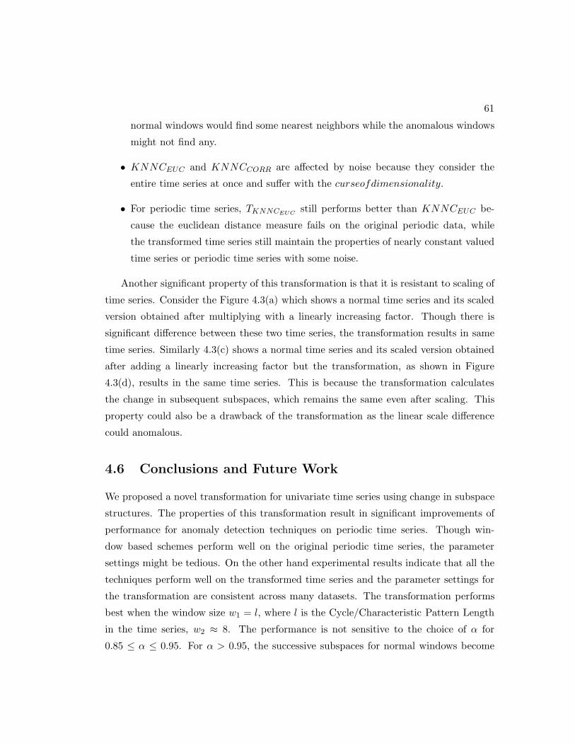
61

normal windows would find some nearest neighbors while the anomalous windows

might not find any.

• KNNCEUC and KNNCCORR are affected by noise because they consider the

entire time series at once and suffer with the curseofdimensionality.

• For periodic time series, TKNNCEUCstill performs better than KNNCEUC be-

cause the euclidean distance measure fails on the original periodic data, while

the transformed time series still maintain the properties of nearly constant valued

time series or periodic time series with some noise.

Another significant property of this transformation is that it is resistant to scaling of

time series. Consider the Figure 4.3(a) which shows a normal time series and its scaled

version obtained after multiplying with a linearly increasing factor. Though there is

significant difference between these two time series, the transformation results in same

time series. Similarly 4.3(c) shows a normal time series and its scaled version obtained

after adding a linearly increasing factor but the transformation, as shown in Figure

4.3(d), results in the same time series. This is because the transformation calculates

the change in subsequent subspaces, which remains the same even after scaling. This

property could also be a drawback of the transformation as the linear scale difference

could anomalous.

4.6 Conclusions and Future Work

We proposed a novel transformation for univariate time series using change in subspace

structures. The properties of this transformation result in significant improvements of

performance for anomaly detection techniques on periodic time series. Though win-

dow based schemes perform well on the original periodic time series, the parameter

settings might be tedious. On the other hand experimental results indicate that all the

techniques perform well on the transformed time series and the parameter settings for

the transformation are consistent across many datasets. The transformation performs

best when the window size w1 = l, where l is the Cycle/Characteristic Pattern Length

in the time series, w2 ≈ 8. The performance is not sensitive to the choice of α for

0.85 ≤ α ≤ 0.95. For α > 0.95, the successive subspaces for normal windows become

62

0 500 1000 1500 2000 2500−5

0

5Original Time Series

0 500 1000 1500 2000 2500−1

−0.5

0

0.5

1x 10

4 Linearly Scaled Time Series

(a) Original and Scaled Time Series obtainedafter multiplying with a linearly increasing fac-tor

0 500 1000 1500 2000 25000

0.5

1Transformation of Original Time Series

0 500 1000 1500 2000 25000

0.5

1Transformation of Scaled Time Series

(b) Transfomation of Original and Scaled TimeSeries

(c) Original and Scaled Time Series obtainedafter adding a linearly increasing factor

(d) Transfomation of Original and Scaled TimeSeries

Figure 4.3: Effect of Transformation on Scaled Time Series

63

unstable and hence result in a high false alarm rate. For α < 0.85, the successive

subspaces for anomalous windows do not differ significantly and hence result in a low

detection rate.

A critical aspect of the proposed technique is the computation of eigen vectors for

the moving window which could become a computational bottleneck, especially when

the dimensionality and length of the time series becomes large. A potential solution is

to update the eigen vectors for sucessive windows incrementally using techniques such

as Matrix Perturbation (90) to avoid computation of the eigen vectors for every window,

and is suggested as a future direction of research.

Chapter 5

Conclusions and Future Work

The existing research on anomaly detection for time series is limited to developing tech-

niques that are suitable for specific application domains. In this thesis we provided

a comprehensive understanding and structured overview of the research on anomaly

detection techniques for time series spanning multiple research areas and application

domains. Each application domain possesses unique characteristics in terms of the data

on which the anomaly detection techniques operate. Our study reveals that the perfor-

mance of the anomaly detection techniques is closely tied to the nature of the underlying

data, and hence the techniques exhibit varying performance across application domains.

The results of our thorough experimental studies for time series data can help a domain

scientist find the technique which is best suited for an application domain.

We also proposed a novel transformation for univariate time series using change in

subspace structures. The properties of this transformation result in significant improve-

ments of performance for anomaly detection techniques on periodic time series. Though

window based schemes perform well on the original periodic time series, the parameter

settings might be tedious. On the other hand, the transformation removes the period-

icity of the time series and highlights the anomalies, hence is a better scheme. Since

the transformation is window based, there is the aspect of redundancy, since successive

windows, are often highly similar to each other and do not provide any additional in-

formation. Removing this redundancy can speed up the performance of the technique.

This aspect of redundancy needs to be understood and is suggested as a future direction

of research. Also as mentioned in chapter 4, computation of eigen vectors for successive

64

65

windows can be made efficient using Matrix Perturbation (90).

Since we are dealing with periodic time series, a direction of future work could be

using signal processing techniques to handle the periodicity of the time series. One can

remove the periodicity from the time series, i.e., transform them using signal processing

techniques, such that the normal and anomalous time series look differently.

The subspace based transformation proposed, though motivated from the work for

multivariate time series anomaly detection, is essentially a transformation from a unvari-

ate time series to another univariate time series. Thus the process of the transformation

could be seen in this perspective and better understood.

References

[1] Arindam Banerjee Varun Chandola and Vipin Kumar. Anomaly detection : A

survey. To Appear in ACM Computing Surveys, 2009.

[2] Eilertson E. Lazarevic A. Tan P.N. Kumar V. Srivastava J. Ertoz, L. and P. Dokas.

Minds - minnesota intrusion detection system. In Data Mining - Next Generation

Challenges and Future Directions. MIT Press., 2004.

[3] Parra L. Spence, C. and P. Sajda. Detection, synthesis and compression in mam-

mographic image analysis with a hierarchical image probability model. In In Pro-

ceedings of the IEEE Workshop on Mathematical Methods in Biomedical Image

Analysis. IEEE Computer Society, Washington, DC, USA, 3, 2001.

[4] Freisleben B. Aleskerov, E. and Rao. Cardwatch: A neural network based database

mining system for credit card fraud detection. In In Proceedings of IEEE Compu-

tational Intelligence for Financial Engineering. 220-226, 1997.

[5] Malik Agyemang, Ken Barker, and Rada Alhajj. A comprehensive survey of nu-

meric and symbolic outlier mining techniques. Intell. Data Anal., 10(6):521–538,

2006.

[6] Victoria Hodge and Jim Austin. A survey of outlier detection methodologies. Artif.

Intell. Rev., 22(2):85–126, 2004.

[7] Arindam Banerjee Varun Chandola and Vipin Kumar. Anomaly detection for

discrete sequences : A survey. Unpublished Work.

[8] F. Chuah, M. C. Fu. Ecg anomaly detection via time series analysis. LECTURE

NOTES IN COMPUTER SCIENCE, pages 123–135.

66

67

[9] S. Akhavan and G. Calva. Automatic anomaly detection in ecg signal by fuzzy

decision making. In In Proceedings of 6th International Conference on Fuzzy Theory

and Technology: Association for Intelligent Machinery, 23-28, 1998.

[10] Sheng Zhang, Amit Chakrabarti, James Ford, and Fillia Makedon. Attack detection

in time series for recommender systems. In KDD ’06: Proceedings of the 12th ACM

SIGKDD international conference on Knowledge discovery and data mining, pages

809–814, New York, NY, USA, 2006. ACM.

[11] David L. Iverson. Inductive system health monitoring. International Conference

on Artificial Intelligence, 2004.

[12] Manuele Bicego and Vittorio Murino. Investigating hidden markov models’ ca-

pabilities in 2d shape classification. IEEE Trans. Pattern Anal. Mach. Intell.,

26(2):281–286, 2004.

[13] Zheng Liu, J.X. Yu, Lei Chen, and Di Wu. Detection of shape anomalies: A proba-

bilistic approach using hidden markov models. IEEE 24th International Conference

on Data Engineering, pages 1325–1327, April 2008.

[14] Li Wei, E. Keogh, and Xiaopeng Xi. Saxually explicit images: Finding unusual

shapes. Data Mining, 2006. ICDM ’06. Sixth International Conference on, pages

711–720, Dec. 2006.

[15] P. Protopapas, J. M. Giammarco, L. Faccioli, M. F. Struble, R. Dave, and

C. Alcock. Finding outlier light-curves in catalogs of periodic variable stars.

MON.NOT.ROY.ASTRON.SOC., 369:677, 2006.

[16] U. Rebbapragada, P. Protopapas, C. E. Brodley, and C. Alcock. Finding anomalous

periodic time series. Submitted to the Machine Learning Journal, 2008.

[17] Haibin Cheng, Pang-Ning Tan, Christopher Potter, and Steven Klooster. Detection

and characterization of anomalies in multivariate time series. In Proceedings of the

ninth SIAM International Conference on Data Mining, 2009.

[18] A. J. Fox. Outliers in time series. Journal of the Royal Statistical Society. Series

B(Methodological), 34(3):350–363, 1972.

68

[19] Junshui Ma and Simon Perkins. Online novelty detection on temporal sequences.

In KDD ’03: Proceedings of the ninth ACM SIGKDD international conference on

Knowledge discovery and data mining, pages 613–618, New York, NY, USA, 2003.

ACM.

[20] Qingtao Wu and Zhiqing Shao. Network anomaly detection using time series anal-

ysis. In Proceedings of the Joint International Conference on Autonomic and

Autonomous Systems and International Conference on Networking and Services,

page 42, Washington, DC, USA, 2005. IEEE Computer Society.

[21] Eamonn Keogh, Jessica Lin, Sang-Hee Lee, and Helga Van Herle. Finding the

most unusual time series subsequence: algorithms and applications. Knowledge

and Information Systems, 11(1):1–27, 2006.

[22] Eamonn Keogh, Jessica Lin, and Ada Fu. Hot sax: Efficiently finding the most

unusual time series subsequence. In Proceedings of the Fifth IEEE International

Conference on Data Mining, pages 226–233, Washington, DC, USA, 2005. IEEE

Computer Society.

[23] NASA DashLink. In https://dashlink.arc.nasa.gov.

[24] E. Keogh and T. Folias. In The ucr time series data mining archive.

[25] A. L. Goldberger et al. Physiobank physiotoolkit and physionet: Components of a

new research resource for complex physiologic signals. 2000.

[26] Deepthi Cheboli Varun Chandola and Vipin Kumar. Detecting anomalies in a time

series database. Technical Report, 09-004.

[27] J. Ma and S. Perkins. Time-series novelty detection using one-class support vector

machines. volume 3, pages 1741–1745 vol.3, 2003.

[28] C. C. Michael and A. Ghosh. Two state-based approaches to program-based

anomaly detection. In ACSAC ’00: Proceedings of the 16th Annual Computer

Security Applications Conference, page 21, Washington, DC, USA, 2000. IEEE

Computer Society.

69

[29] Zhang J, Tsui FC, Wagner MM, and Hogan WR. Detection of outbreaks from time

series data using wavelet transform. AMIA Annu Symp Proc, 2003.

[30] Thomas Lotze, Galit Shmueli, Sean Murphy, and Howard Burkom. A wavelet-based

anomaly detector for early detection of disease outbreaks. 2008.

[31] Y. Qiao, X. W. Xin, Y. Bin, and S. Ge. Anomaly intrusion detection method based

on hmm. Electronics Letters, 38(13):663–664, 2002.

[32] Xiaoqiang Zhang, Pingzhi Fan, and Zhongliang Zhu. A new anomaly detection

method based on hierarchical hmm. In Proceedings of the 4th International Confer-

ence on Parallel and Distributed Computing, Applications and Technologies, pages

249–252, 2003.

[33] Philip K. Chan and Matthew V. Mahoney. Modeling multiple time series for

anomaly detection. In Proceedings of the Fifth IEEE International Conference on

Data Mining, pages 90–97, Washington, DC, USA, 2005. IEEE Computer Society.

[34] Matthew V. Mahoney and Philip K. Chan. Trajectory boundary modeling of time

series for anomaly detection. In Proceedings of the KDD Workshop on Data Mining

Methods for Anomaly Detection, 2005.

[35] Stan Salvador and Philip Chan. Learning states and rules for detecting anomalies

in time series. Applied Intelligence, 23(3):241–255, 2005.

[36] Li Wei, Nitin Kumar, Venkata Lolla, Eamonn J. Keogh, Stefano Lonardi, and

Chotirat Ratanamahatana. Assumption-free anomaly detection in time series.

In Proceedings of the 17th international conference on Scientific and statistical

database management, pages 237–240, Berkeley, CA, US, 2005. Lawrence Berkeley

Laboratory.

[37] Jessica Lin, Eamonn Keogh, Stefano Lonardi, and Bill Chiu. A symbolic represen-

tation of time series, with implications for streaming algorithms. In DMKD ’03:

Proceedings of the 8th ACM SIGMOD workshop on Research issues in data mining

and knowledge discovery, pages 2–11, New York, NY, USA, 2003. ACM.

70

[38] Eamonn Keogh, Kaushik Chakrabarti, Sharad Mehrotra, and Michael Pazzani.

Locally adaptive dimensionality reduction for indexing large time series databases.

In In proceedings of ACM SIGMOD Conference on Management of Data, pages

151–162, 2001.

[39] Eamonn Keogh, Stefano Lonardi, and Bill ’Yuan chi’ Chiu. Finding surprising

patterns in a time series database in linear time and space. In Proceedings of the

eighth ACM SIGKDD international conference on Knowledge discovery and data

mining, pages 550–556, New York, NY, USA, 2002. ACM Press.

[40] Stephanie Forrest and Dipankar Dasgupta. Novelty detection in time series data

using ideas from immunology. In Proceedings of the 5th International Conference

on Intelligence Systems, Reno, Nevada, USA, 1996. IEEE Computer Society.

[41] Vipin Kumar Pang-Ning Tan, Michael Steinbach. Introduction to data mining.

[42] Xiao yun Chen and Yan yan Zhana. Multi-scale anomaly detection algorithm

based on infrequent pattern of time series. Journal of Computational and Applied

Mathematics, 214(1):227–237, April 2008.

[43] Ada Wai-Chee Fu, Oscar Tat-Wing Leung, Eamonn J. Keogh, and Jessica Lin.

Finding time series discords based on haar transform. In Proceeding of the 2nd

International Conference on Advanced Data Mining and Applications, pages 31–

41. Springer Verlag, 2006.

[44] Y. Bu, T-W Leung, A. Fu, E. Keogh, J. Pei, and S. Meshkin. Wat: Finding

top-k discords in time series database. In Proceedings of 7th SIAM International

Conference on Data Mining, 2007.

[45] Kin-Pong Chan and Ada Wai-Chee Fu. Efficient time series matching by wavelets.

Data Engineering, 1999. Proceedings., 15th International Conference on, pages

126–133, Mar 1999.

[46] Cyrus Shahabi, Xiaoming Tian, and Wugang Zhao. Tsa-tree: A wavelet-based

approach to improve the efficiency of multi-level surprise and trend queries on time

series data. In Proceedings of the 12th International Conference on Scientific and

71

Statistical Database Management, page 55, Washington, DC, USA, 2000. IEEE

Computer Society.

[47] Cyrus Shahabi, Seokkyung Chung, Maytham Safar, and George Hajj. 2d tsa-

tree: A wavelet-based approach to improve the efficiency of multi-level spatial

data mining. In Proceedings of the 13th International Conference on Scientific and

Statistical Database Management, page 59, Washington, DC, USA, 2001. IEEE

Computer Society.

[48] Michail Vlachos, Marios Hadjieleftheriou, Dimitrios Gunopulos, and Eamonn

Keogh. Indexing multi-dimensional time-series with support for multiple distance

measures. In KDD ’03: Proceedings of the ninth ACM SIGKDD international con-

ference on Knowledge discovery and data mining, pages 216–225, New York, NY,

USA, 2003. ACM.

[49] B. Abraham and A. Chuang. Outlier detection and time series modeling. Techno-

metrics, 31(2):241–248, 1989.

[50] B. Abraham and G. E. P. Box. Bayesian analysis of some outlier problems in time

series. Biometrika, 66(2):229–236, 1979.

[51] Chris Chatfield. The analysis of time series : an introduction. Chapman and Hall

CRC, 6th edition, 2004.

[52] Ryohei Fujimaki, Takehisa Yairi, and Kazuo Machida. An anomaly detection

method for spacecraft using relevance vector learning. Advances in Knowledge

Discovery and Data Mining, 3518:785–790, 2005.

[53] B. Pincombe. Anomaly detection in time series of graphs using arma processes.

ASOR BULLETIN, 24(4):2–10, 2005.

[54] H. Zare Moayedi and M.A. Masnadi-Shirazi. Arima model for network traffic pre-

diction and anomaly detection. International Symposium on Information Technol-

ogy, 4:1–6, Aug. 2008.

[55] F. Knorn and D.J. Leith. Adaptive kalman filtering for anomaly detection in

72

software appliances. IEEE Conference on Computer Communications Workshops,

pages 1–6, April 2008.

[56] David Moore and George McCabe. Introduction to the Practice of Statistics. 5th

edition, 2004.

[57] Carl Edward Rasmussen. Gaussian processes in machine learning. Machine Learn-

ing Summer School, 2003.

[58] Vladimir N. Vapnik. The nature of statistical learning theory. Springer-Verlag New

York, Inc., New York, NY, USA, 1995.

[59] Christopher Bishop. Pattern Recognition and Machine Learning. Springer Science

Business Media LLC, 2006.

[60] L. Rabiner and B. Juang. An introduction to hidden markov models. ASSP Mag-

azine, IEEE, 3(1):4–16, Jan 1986.

[61] Veselina Jecheva. About some applications of hidden markov model in intrusion

detection systems. In International Conference on Computer Systems and Tech-

nologies - CompSysTech, 2006.

[62] Shrijit S. Joshi and Vir V. Phoha. Investigating hidden markov models capabilities

in anomaly detection. In ACM-SE 43: Proceedings of the 43rd annual Southeast

regional conference, pages 98–103, New York, NY, USA, 2005. ACM.

[63] Hai-Tao He and Xiao-Nan Luo. A novel hmm-based approach to anomaly detection.

2004.

[64] Ninad Thakoor and Jean Gao. Hidden markov model based 2d shape classification,

2005.

[65] Leonard E. Baum, Ted Petrie, George Soules, and Norman Weiss. A maximization

technique occurring in the statistical analysis of probabilistic functions of markov

chains. The Annals of Mathematical Statistics, 41(1):164–171, 1970.

[66] Eamonn J. Keogh, Selina Chu, David Hart, and Michael J. Pazzani. An online

algorithm for segmenting time series. In ICDM ’01: Proceedings of the 2001 IEEE

73

International Conference on Data Mining, pages 289–296, Washington, DC, USA,

2001. IEEE Computer Society.

[67] William W. Cohen. Fast effective rule induction. In In Proceedings of the Twelfth

International Conference on Machine Learning, pages 115–123. Morgan Kaufmann,

1995.

[68] Jamal Ameen and Rawshan Basha. Mining time series for identifying unusual sub-

sequences with applications. In ICICIC ’06: Proceedings of the First International

Conference on Innovative Computing, Information and Control, pages 574–577,

Washington, DC, USA, 2006. IEEE Computer Society.

[69] Basha R and Ameen JRM. Unusual sub-sequence identifications in time series

with periodicity. In IJICIC ’07: International Journal on Innovative Computing,

Information and Control, volume 3, 2007.

[70] Jamal Ameen and Rawshan Basha. Hierarchical data mining for unusual sub-

sequence identifications in time series processes. In Proceedings of the Second In-

ternational Conference on Innovative Computing, Information and Control, page

177, Washington, DC, USA, 2007. IEEE Computer Society.

[71] G. Keshav Palshikar. Distance-based outliers in sequences. 3816/2005.

[72] E. Keogh, J. Lin, A.W. Fu, and H. VanHerle. Finding unusual medical time-

series subsequences: Algorithms and applications. Information Technology in

Biomedicine, IEEE Transactions on, 10(3):429–439, July 2006.

[73] Ashok N. Srivastava. Discovering system health anomalies using data mining tech-

niques. In Proceedings of 2005 Joint Army Navy NASA Airforce Conference on

Propulsion, 2005.

[74] Ling Huang, Xuanlong Nguyen, Minos Garofalakis, Michael Jordan, Anthony

Joseph, and Nina Taft. In-network pca and anomaly detection. Technical sup-

port, U.C. Berkeley, Berkeley, CA, 01/2007 2007.

[75] Varun Chandola. Anomaly detection for symbolic sequences and time series data

: Ph.d dissertation.

74

[76] M. Basseville, M. Abdelghani, and A. Benveniste. Subspace-based fault detection

algorithms for vibration monitoring. Automatica, 36:101–109, 2000.

[77] Manabu Kano, Shinji Hasebea, Iori Hashimotoa, and Hiromu Ohno. A new multi-

variate statistical process monitoring method using principal component analysis.

Computers & Chemical Engineering, 25(7–8):1103–1113, 2001.

[78] C. Jordan. Essai sur la geometrie a n dimensions. Buletin de la Societe Mathema-

tique de France, 3:103–174, 1875.

[79] H. Hotelling. Relation between two sets of variates. Biometrika, 28:322–377, 1936.

[80] K. De Cock and B. De Moor. Subspace angles between arma models. Systems and

Controls Letters, 46(4):265–270, July 2002.

[81] Jeroen Boets, K. De Cock, M. Espinoza, and B. De Moor. Clustering time series,

subspace identification and cepstral distances. Communications in Information

Systems, 5(1):69–96, 2005.

[82] Dragomir Yankov, Eamonn J. Keogh, and Umaa Rebbapragada. Disk aware discord

discovery: Finding unusual time series in terabyte sized datasets. In Proceedings

of International Conference on Data Mining, pages 381–390, 2007.

[83] D. Berndt and J. Clifford. Using dynamic time warping to find patterns in time

series. In AAAI Workshop on Knowledge Discovery in Databases, pages 229–248,

1994.

[84] P. Protopapas, J. M. Giammarco, L. Faccioli, M. F. Struble, R. Dave, and C. Al-

cock. Finding outlier light curves in catalogues of periodic variable stars. Monthly

Notices of the Royal Astronomical Society, 369(2):677–696, 2006.

[85] Stephanie Forrest, Christina Warrender, and Barak Pearlmutter. Detecting intru-

sions using system calls: Alternate data models. In Proceedings of the 1999 IEEE

ISRSP, pages 133–145, Washington, DC, USA, 1999. IEEE Computer Society.

[86] Klaus-Robert Muller, Alex J. Smola, Gunnar Ratsch, Bernhard Scholkopf, Jens

Kohlmorgen, and Vladimir Vapnik. Predicting time series with support vector

75

machines. In Proceedings of the 7th International Conference on Artificial Neural

Networks, pages 999–1004, London, UK, 1997. Springer-Verlag.

[87] V. Chandola, V. Mithal, and V. Kumar. A comparative evaluation of anomaly

detection techniques for sequence data. In Proceedings of International Conference

on Data Mining, 2008.

[88] Shyam Boriah. Time series change detection: Algorithms for land cover change :

Ph.d dissertation.

[89] Ashok Srivastava. Nasa dashlink. https://dashlink.arc.nasa.gov, 2008.

[90] G. W. Steward and Ji guang Sun. Matrix Perturbation Theory. Academic Press,

1990.

Documents

Anomaly Detection of Time Series