Embed Size (px)
Citation preview

Anomalous Transport in Chiral
Systems
A Dissertation Presented
by
Gustavo Machado Monteiro
to
The Graduate School
in Partial Fulfillment of the Requirements
for the Degree of
Doctor of Philosophy
in
Physics
Stony Brook University
July 2016

Stony Brook University
The Graduate School
Gustavo Machado Monteiro
We, the dissertation committee for the above candidate for the Doctor ofPhilosophy degree, hereby recommend acceptance of this dissertation.
Dr. Alexander G. Abanov – Dissertation AdvisorProfessor, Department of Physics and Astronomy
Dr. Dmitri E. Kharzeev – Co-AdvisorProfessor, Department of Physics and Astronomy
Dr. Ismail Zahed – Chairperson of DefenseProfessor, Department of Physics and Astronomy
Dr. Xu Du – Committee MemberProfessor, Department of Physics and Astronomy
Dr. Alexei Tsvelik – Outside MemberCondensed Matter Physics and Materials Science Department, Brookhaven
National Laboratory
This dissertation is accepted by the Graduate School.
Nancy Goro↵Interim Dean of the Graduate School
ii

Abstract of the Dissertation
Anomalous Transport in Chiral Systems
by
Gustavo Machado Monteiro
Doctor of Philosophy
in
Physics
Stony Brook University
2016
The experimental realization of Dirac and Weyl semimetals in 2014and 2015 respectively has increased the interest in the topic. Sim-ilarly to graphene, the discovered materials are characterized bymassless quasiparticles. In three dimensions these quasiparticlescan be described by the Weyl Hamiltonian which exhibits so-calledchiral anomaly at low energies. The chiral anomaly has a transportsignature, namely, the enhancement of longitudinal conductivityalong the direction of external magnetic field. This e↵ect in newmaterials is the condensed matter version of the chiral magnetice↵ect (CME) predicted to happen in heavy ion collisions. Due toits topological nature the chiral anomaly it is believed to be robustwith respect to the interaction strength and anomalous contribu-tion to transport is believed to be universal and independent of theinteraction.
This thesis is devoted to the study of magnetotransport in Diracand Weyl metals. For that, we use the chiral kinetic theory todescribe within the same framework both the negative magnetore-sistance caused by chiral magnetic e↵ect and quantum oscillations
iii

in the magnetoresistance due to the existence of the Fermi sur-face. In the second part, we refer to the hydrodynamics with gaugeanomaly and study the non-dissipative transport using variationalprinciple as a main tool. In the last part of the Thesis we also applyvariational approach to study the Hall viscosity in two-dimensionalsystems.
iv

Publications1. Gustavo M. Monteiro and Alexander G. Abanov. Variational Principle
for Hall FluidsIn preparation
2. Gustavo M. Monteiro, Alexander G. Abanov, and Dmitri E. Kharzeev.Magnetotransport in Dirac metals: Chiral magnetic e↵ect and quantumoscillations. Phys. Rev. B, 92 (165109), Oct 2015.
3. Gustavo M. Monteiro, Alexander G Abanov, and V. P. Nair. Hydro-dynamics with gauge anomaly: Variational principle and hamiltonianformulation. Phys Rev D, 91(125033), 2015.
v


Contents
List of Figures ix
Acknowledgements x
1 Introduction 11.1 Thesis Outline . . . . . . . . . . . . . . . . . . . . . . . . . . . 11.2 Weyl and Dirac Semimetals . . . . . . . . . . . . . . . . . . . 2
1.2.1 Two-band System: An Example . . . . . . . . . . . . . 31.2.2 Nielsen-Ninomiya Theorem . . . . . . . . . . . . . . . . 51.2.3 Fermi Arcs . . . . . . . . . . . . . . . . . . . . . . . . . 7
1.3 Anomalous Hydrodynamics . . . . . . . . . . . . . . . . . . . 91.3.1 The Chiral Magnetic E↵ect (CME) . . . . . . . . . . . 10
1.4 Hall Fluid . . . . . . . . . . . . . . . . . . . . . . . . . . . . . 121.5 Clebsch Parametrization . . . . . . . . . . . . . . . . . . . . . 13
1.5.1 Non-relativistic Hydrodynamic Action . . . . . . . . . 151.5.2 Entropy Conservation . . . . . . . . . . . . . . . . . . 161.5.3 Relativistic Hydrodynamic Action . . . . . . . . . . . . 17
2 Magnetotransport in Dirac and Weyl Metals 192.1 Semiclassical Dynamics . . . . . . . . . . . . . . . . . . . . . . 192.2 Chiral Kinetic Theory . . . . . . . . . . . . . . . . . . . . . . 242.3 Boltzmann Equation . . . . . . . . . . . . . . . . . . . . . . . 262.4 Interplay Between CME and SdH E↵ect . . . . . . . . . . . . 29
3 Hydrodynamics with Gauge Anomaly 333.1 Constitutive Relations . . . . . . . . . . . . . . . . . . . . . . 343.2 Hydrodynamic Action . . . . . . . . . . . . . . . . . . . . . . 353.3 Symmetries . . . . . . . . . . . . . . . . . . . . . . . . . . . . 383.4 Hamiltonian Formalism . . . . . . . . . . . . . . . . . . . . . . 403.5 Poisson Brackets . . . . . . . . . . . . . . . . . . . . . . . . . 413.6 Symmetry generators . . . . . . . . . . . . . . . . . . . . . . . 44
vii

4 Odd Viscosity from Variational Principle 474.1 Odd Viscosity Ambiguity . . . . . . . . . . . . . . . . . . . . . 474.2 Gradient Corrections to the Perfect Fluid Action . . . . . . . 494.3 Newton-Cartan Geometry . . . . . . . . . . . . . . . . . . . . 514.4 Hydrodynamics in Newton-Cartan Background . . . . . . . . . 534.5 Symmetries in Newton-Cartan Geometry . . . . . . . . . . . . 55
5 Future Directions: Transport Properties of Topological Sur-face States 575.1 Chiral Kinetic Theory with Fermi Arcs . . . . . . . . . . . . . 575.2 Boundary Modes in Anomalous Hydrodynamics . . . . . . . . 58
Bibliography 60
A Poisson Summation Formula and SdH E↵ect 65
B Dingle Factor 70
C Sympletic Form and Poisson Structure 73
D Hamiltonian Equations for Hydrodynamic with Anomalies 76
viii

List of Figures
1.1 Examples of dispersion relations for a) type-I and b) type-IIWeyl semimetals. These plots were extracted from [1]. . . . . 4
2.1 Semiclassical picture of Fermi surface for right and left chiralmodes is shown in the presence of the magnetic field. For thelinear dispersion, the support of Hamiltonian eigenstates is acollection of cylinders corresponding to eigenvalues "⌫(kz) =~vF
p
k2
z + k2
?, where k2
? = 2eB⌫ with ⌫ 2 Z+
. The state with⌫ = 0 is chiral and exists only for kz > 0 (parallel to B) for theright chirality and for kz < 0 for the left one. . . . . . . . . . . 23
2.2 Longitudinal magnetoresistance as a function of the magneticfield. On the left: the results of experiment [2] on Cd
3
As2
.On the right: the results of computation [3] with numericalparameters kF = 3.8 ⇥ 108m�1, vF = 9.3 ⇥ 105m/s, ⌧ = 8 ⇥10�13s, T = 2.5K. The plots are made for three values of thequantum lifetime ⌧Q/⌧ = 0, 1, 16 and for the chirality relationtime ⌧v = 10⌧ . . . . . . . . . . . . . . . . . . . . . . . . . . . 31
2.3 Magnetoresistence in TaP, the plot in a) was extracted from [4],whereas the plot in b) was taken from [5]. . . . . . . . . . . . 32
ix

Acknowledgements
First of all, I would like to apologize in advance for my unfairness, there aresome silent voices that should be here, yet they did not make it into thisacknowledgment.
I would like to express my gratitude and my admiration to both of myadvisors and two of the best teachers in Stony Brook: Sasha Abanov andDima Kharzeev. I would like to thank Sasha for his patience and guidancethroughout these 4 years and most importantly for always treating me as ayoung collaborator instead of a PhD student. This kept me motivated evenwhen I was stuck in our first project together. I hope I can show in my futureresearch career how much I have learnt from him and his physics intuition/un-derstanding. I would like to express my gratitude to Dima for the financialsupport when my fellowship ended, and most importantly for teaching me,in the last 2 years of my PhD, how to do high-level research. Due to him, Istarted to read experimental papers and I hope one day I will have some ofthe ability he has to cover di↵erent areas physics. If I could not do more inthis PhD, it was solely due to my limitations and stubbornness.
Besides them, I would like to express my gratitude to past and poten-tially future collaborators: V. P. Nair, Andrey Gromov, Tankut Can, NickTarantino, Andrea Massari, Kristan Jensen and Pasha Wiegmann for all theuseful discussions.
Sono moltissimo grato a la Giulia por questi 3 anni in sieme e per i 6 annidi amista. Grazie per tanti ricordi carini e per essere questa persona veramenteraggiante che “contagia” a tutti la gente, quando non ha fame. Meus agradec-imentos a Luana, pois sua amizade foi o maior legado que Stony Brook meproporcionou. Muito obrigado por sempre estar la quando precisei, mesmo queacompanhada de inumeras e corriqueiras reclamacoes. Mi profundos agradec-imientos a mi “hermano” Jose Cordova. Uno de mi pilares de sustentaciondurante estes 6 anos, siempre a mi lado con sus consejos siempre valiosos y susmomentos de valley girl.
Amigos sao aqueles nos quais sempre podemos contar, mesmo quando esta-mos errados. Por isso minha imensa gratidao ao sempre sorridente e energetico
x

Gabriel, parceiro para todas as horas, seja nos momentos de diversao e descon-tracao, seja nos problems mais complicados. Mi eterna gratitud a Ruth y JosePalomino, que me hicieran padrino de su hijo Jose Ramon. Apesar de “cu-sones” asumidos, nos tornamos grandes amigos en tan poco tiempo que losquiero como mi famılia.
I would like to thank Maria for our conservations and for being such acaring person, she has always made me feel at home in a foregn country. It issuch a pity we will never see each other again. I would love to also thank JoePuripant for being such a great company throughout these 6 years, but sadlywe do not do that. Mis agradecimientos al mi par de “weones” favoritos, pornuestra amistad que 2 anos y 8190 km no fueran capaces de cambiar. Fue unhonor haber sido su padrino de matrimonio.
Mi gratitud a mis grandes amigos espanoles Sara, Inigo y Adrian y a miamigo nuevayorkino/pueltoliqueno/consumado en Mexico Doug por todos losmomentos de diversion, las borracheras y asereje ja de je de jebe tu de jebereseibiunouva majavi an de bugui an de guididıpi.
I would like thank my friends from the Maine trip, since I told them Iwould... Betul and Murat, for being such a pleasant couple to spend sometime with, making it impossible to be bored around them. Sriram and Divya,for the great advices and profound conversations. Tatsiana, Vasily and theirability to keep an interesting conversation in any topic.
I would also like to thank the Schomburg crew: Mamal, Harris, Tomas, Leniand Laszlo for such for so many memories and fun nights. Mis agradecimientosa Maria Mera y Luıs Chiang por los finales de semanas llenos de risas, “¡PorDios, Gustavo!” y “¿Das ı?”.
Minha gratidao a todos os amigos das antigas, mas principalmente a Yuri,ao Naga, ao Neto e a Bia por serem meu porto seguro, aqueles nos quais eusempre posso contar e confiar cegamente. Felizes daqueles que encontraramem suas vidas amigos como eles. Meus agradecimentos ao Gui, ao Gu e aoGlauber por nunca deixarem nossa amizade envelhecer junto conosco.
Meus profundos e mais sinceros agradecimentos a toda minha famılia, emespecial a meus pais que sempre me apoiaram, mesmo que isso significasseter seu filho preferido a milhares de quilometros de distancia. Se cheguei ateonde cheguei, eles foram os culpados, pois ninguem aprende a andar sozinhoe, apesar de estarem sempre ao meu redor para me segurar caso eu caia, essesforam meus primeiros sem segurar suas maos. Por fim, minha gratidao a minhaeterna cumplice e melhor amiga Thaıs que souber ser tudo isso sem deixar deser minha caculinha. Minha irmazinha mais nova que ja me socorreu tantasvezes e souber ser minha irma mais velha sempre que preciso, e varias vezesdesnecessariamente.
xi

The last, but not the least, I would like thank CAPES and Fulbright forthe financial support.
xii

Chapter 1
Introduction
1.1 Thesis Outline
This thesis is organized in a way that one chapter is completely independentof each other. The underlying connection between them is traced in the intro-duction, where the di↵erent topics are tied together, even though the actualpieces of the work may seem distinct.
At chapter 2, we will study the longitudinal magnetoconductivity of Diracand Weyl metals by analytically computing the Boltzmann equation. Mo-tivated by the experiments on Cd
3
As2
, we will study the interplay betweenthe Shubnikov-de Haas e↵ect with the negative magnetoresistance due to thechiral anomaly at low energies. This chapter allows for a direct comparisonto the experimental data and is based on the published work [3] of the PhDcandidate.
Chapter 3 is more formal and has no direct connection to experiments. Wewill construct the variational principle for the hydrodynamic equations withgauge anomaly, focusing on the symmetry properties and the mathematicalstructure of the problem. This chapter corresponds to the work done by thePhD candidate in [6]. At chapter 4, we will study Hall viscosity terms in thehydrodynamics from a variation principle. We will fix any ambiguity in defin-ing conserved currents by introducing background fields from Newton-Cartangeometry. Both chapters 3 and 4 rely on the so-called Clebsch parametrization,which will be explained in the section 1.5.
In the last chapter, about other ongoing projects, we will present a conver-gence point between both published pieces of work [3] and [6]. Such connectionrely on the transport properties of topologically protected surface states inboth kinetic theory and hydrodynamics. In the section 5.2, we will discuss theexistence of hydrodynamic surface modes, which can have some implication
1
on the study of Fermi arcs in Weyl and Dirac semimetals.
1.2 Weyl and Dirac Semimetals
Throughout the last decade, we have succeeded in including the adjectivetopological to various states of matter. Two ground states are topologicallyequivalent if and only if we can adiabatically deform one into the other withoutbreaking any of the underlying symmetries. As an example, any conventionalinsulator can be continuously connected to non-interacting atoms arranged ina lattice. In a particular tight-binding model, this can be done by settingthe hopping parameter to zero. This definition relies on validity of the adi-abatic theorem and is thus restricted to gapped systems. In general, gaplessphases occur in the quantum phase transition between two distinct topolog-ical phases, where the adiabatic theorem breaks down. They are said to beunstable when the gap closes only at the quantum critical point and stablewhen gap remains closed for a finite interval in the parameter space [7]. Diracsemimetals can be seen as an intermediate phase in between the trivial andthe topological insulator phases of the same material, where the gap closes atisolated points in the Brillouin zone. The most well-known example is the com-pound ZrTe
5
which was predicted to be a 3D quantum spin Hall insulator [8],though transport and ARPES measurements have shown that it behaves in-stead as a Dirac semimetal [9]. The e↵ective low-energy Hamiltonian for Diracsemimetals is invariant under time-reversal and inversion symmetry, and itsquasiparticle excitations form a Kramer’s doublet. Weyl semimetals can beobtained from Dirac semimetals by breaking either time reversal or inversionsymmetry, which splits the Dirac point into two band-touching (Weyl) pointswith opposite chiralities.
Dirac semimetals were only experimentally realized in 2014, and the firstsynthesized compounds were Cd
3
As2
[10–12], Na3
Bi [13] and ZrTe5
[9]. Ex-perimental data have shown that these materials are characterized by largemobility and high magnetoresistance, which are mostly but not fully under-stood. Although proposed before the Dirac semimetals, Weyl semimetals haveproven to be more challenging to be realized experimentally, being synthe-sized only in 2015. There are only four Weyl semimetals known to date, theseare TaAs [14, 15], TaP [16], NbAs [17] and NbP. In addition to that, Weylsemimetals are characterized by topologically protected surface states, calledFermi arcs [16–19]. Fermi arcs connect two disjoint pieces of Fermi surfacewith opposite chirality. In the case of Dirac semimetals, such Fermi arcs arenot topologically protected and can hybridize into a closed Fermi loop on thesurface [20].
2

For the sake of simplicity, we will describe Weyl semimetals in the nextsubsection in terms of a two-band model system. Dirac semimetals can beunderstood as two copies of Weyl semimetals connected by time-reversal sym-metry.
1.2.1 Two-band System: An Example
The most general two-band system Hamiltonian can be written as:
H(k) = b0
(k) I2⇥2
+ b(k) · �, (1.1)
where (b0
, b) are real functions of the crystal quasimomentum k and � is thevector whose components are the Pauli matrices. The symmetries of suchBloch Hamiltonian can be extracted from the microscopics1:
T : H⇤(k) = H(�k), (1.2)
I : H(k) = H(�k), (1.3)
where T is the time-reversal operator and I is the lattice inversion. A two-band system is only IT-invariant when b
2
(k) = 0, and the other real functionsare even in k. Band-touching points occur when b
1
(k0) = b3
(k0) = 0, forsome k0 in the Brillouin zone. Since b
1,3(k) = 0 correspond to surfaces onthe three-dimensional Brillouin zone, their intersection defines either lines orkissing points. Therefore, one cannot obtain a Weyl semimetal from a IT-invariant system2. For systems with broken IT, the Bloch Hamiltonian (1.1)becomes non-real and the Weyl points occur when the equation
b1
(ka
) = b2
(ka
) = b3
(ka
) = 0
admits solutions for a discrete set of points {ka
} in the Brillouin zone. Whenthe Fermi energy lies near the energy of a Weyl point k0 2 {k
a
}, we canlinearize the Hamiltonian around such point. If we set the Weyl point energyto be zero, the e↵ective Hamiltonian can be written as:
H(k) = (I2⇥2
⌫j + �ivij) (�k)j, (1.4)
1The equation (1.2) is only true when the quasiparticle does not belong to a Kramer’sdoublet, i.e., it is a singlet under T.
2The quasiparticle dispersion relation will be flat in at least one direction. More sys-tematically, one can show that Berry phase of Bloch states away from the band-touchingpoints vanishes for a IT-invariant system.
3

where
⌫j =@b
0
@kj
�
�
�
�
k0
, (1.5)
vij =@bi@kj
�
�
�
�
k0
, (1.6)
�k = k � k0. (1.7)
The zero-energy solutions of the Hamiltonian (1.4) fall into two classes: asingle Weyl point at k = k0; or a band-touching point at k = k0 connectingtwo disjoint pieces of Fermi surface, one filled by hole states and the other byelectron quasiparticles. The former is a characteristic of type-I Weyl semimet-als and the latter describes the recently discovered type-II Weyl semimetals[1]. The dispersion relations for both cases is represented in Fig. 1.1.
Figure 1.1: Examples of dispersion relations for a) type-I and b) type-II Weylsemimetals. These plots were extracted from [1].
Let us ignore the time-reversal symmetry for now and impose only the in-version symmetry. If b(k) vanishes for some k0 in the Brillouin zone, equation(1.3) imposes that necessarily b(�k0) = 0 and that both Weyl points are atthe same energy. Assuming that there are only two band touching points, thelow-energy e↵ective Hamiltonian becomes:
Heff (k) = H+
(k) � H�(k), (1.8)
where H±(k) are the linearized Hamiltonians expanded at ±k0. They can beexpressed as:
H±(k) = ± (I2⇥2
⌫j + �ivij) [kj ⌥ (k0
)j]. (1.9)
4

We have again set the Weyl points to be at zero energy. The chirality of the
Weyl quasiparticle is defined by the sign of det⇣
@bi@kj
⌘
evaluated at the Weyl
point. Invariance over I imposes that the Weyl points have opposite chirality,since:
det (�vij) = � det vij.
Let us repeat the analysis for a system with broken inversion symmetry,yet invariant under time-reversal. If there is a Weyl point at k0, so will therebe another one at �k0. However, equation (1.2) show us that the Weyl pointshave the same chirality. Nielsen-Ninomiya theorem states that the existence ofonly Weyl points of the same chirality is inconsistent with lattice symmetries[21]. In other words, Weyl point must come in pairs of opposite chirality asit will be shown in the next section. Therefore the smallest number of Weylpoints in a T-invariant system with broken I is four.
1.2.2 Nielsen-Ninomiya Theorem
In this section, we will review the Nielsen-Ninomiya theorem, also known aslattice doubling theorem. It was first introduced in [21], where the authorsconsidered a system of Weyl fermions on a lattice coupled to a gauge field.The Nielsen-Ninomiya theorem states that Weyl points must come in pairsand with opposite chiralities. In a more modern jargon, the total Berry fluxacross all disjoint pieces of Fermi surface must vanish.
Let us consider the Hamiltonian (1.1) and assume that band-touchingpoints form discrete set of points {k
a
} in the Brillouin zone, BZ. For allother points in the Brillouin zone, there is a gap between bands3. Neither thegap nor the positions of the Weyl points depend on the the function b
0
(k).Therefore, the bands can be labeled by eigenstates of:
h(k) = � · b(k)
|b(k)| , (1.10)
Obviously, this operator is not defined for the points {ka
}. Away fromthese points the eigenvalues of such operator are ±1, where �1 corresponds tothe “valence band” and +1 labels the “conduction band”. The domain of suchoperation is the reduced Brillouin zone BZ 0 with such bad points removed.
3One can view this two-band system as a two-level system at each point in the Brillouinzone.
5
Formally, this reduced Brillouin zone is defined as:
BZ 0 = BZ \[
↵
U↵,
where each U↵ is a small open set around the Weyl point k↵. The equation
h(k)|u±k
i = ±|u±k
i, (1.11)
defines what we call line bundles. In principle, a general state can be viewedas a C2-vector at each point in BZ 0. The Hilbert space4 for states that satisfyequation (1.11) are split into a direct sum H
k
⇠= C�C. If we restrict ourselvesto positive eigenvalue states of (1.11), we define a line bundle5 over BZ 0, since↵|u±
k
i, with ↵ 2 C, is still a positive eigenvalue state of h(k).The normalization condition fixes the modulus of |u+
k
i, however its phasecannot be fixed by any of these arguments. This reduces the line bundle to aU(1) principal bundle over the Brillouin zone. In physical terms, this meansthat we can always multiply the state by a local phase, that is,
|u+
k
i ! ei'(k)|u+
k
i. (1.12)
Let us consider now a path on the Brillouin zone. The normalizationcondition imposes that along the path:
hu+
k
| dds
u+
k
i = 0. (1.13)
This defines how the phase is parallel transported on the U(1) principlebundle. In other words,
d
ds|u+
k
i ⌘ dk
ds· [r
k
+ iA(k)] |u+
k
i, (1.14)
where A(k) is the Berry connection over the U(1)-bundle. Contracting thisequation with hu+
k
|, we obtain:
A(k) = ihu+
k
|rk
u+
k
i. (1.15)
Under the “gauge” transformation (1.12), the Berry connection transformsas:
A ! A+rk
' . (1.16)
4The total Hilbert space should be understood as H ⇠=R �
BZ Hk dµ(k).5A manifold which is locally isomorphic to C ⇥ U , where U is an open set of BZ 0
6
In analogy with the electromagnetism, the gauge invariant quantity is theBerry curvature, defined as:
⌦ ⌘ rk
⇥ A . (1.17)
Thus,r
k
· ⌦ = 0, 8k 2 BZ 0. (1.18)
Integrating (1.18) over the whole domain and using the Stokes theorem,we find that:
X
↵
Z
@ U↵
⌦ · dS =X
↵
c1
(@ U↵) = 0, (1.19)
Therefore, Weyl points correspond to monopole solutions of the Berry cur-vature and the total monopole charge (Chern number) must vanish. Thegeneral proof for a many-band system can be found at [22].
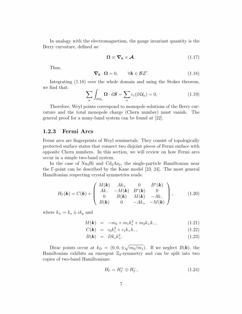
1.2.3 Fermi Arcs
Fermi arcs are fingerprints of Weyl semimetals. They consist of topologicallyprotected surface states that connect two disjoint pieces of Fermi surface withopposite Chern numbers. In this section, we will review on how Fermi arcsoccur in a simple two-band system.
In the case of Na3
Bi and Cd3
As2
, the single-particle Hamiltonian nearthe �-point can be described by the Kane model [23, 24]. The most generalHamiltonian respecting crystal symmetries reads:
H�
(k) = C(k) +
0
B
B
@
M(k) Ak+
0 B⇤(k)Ak� �M(k) B⇤(k) 00 B(k) M(k) �Ak�
B(k) 0 �Ak+
�M(k)
1
C
C
A
, (1.20)
where k± = kx ± iky and
M(k) = �m0
+m1
k2
z +m2
k+
k�, (1.21)
C(k) = c0
k2
z + c1
k+
k�, (1.22)
B(k) = Dkzk2
+
. (1.23)
Dirac points occur at kD = (0, 0,±p
m0
/m1
). If we neglect B(k), theHamiltonian exhibits an emergent Z
2
-symmetry and can be split into twocopies of two-band Hamiltonians:
H�
= H+
�
� H��
, (1.24)
7

where,H±
�
= C(k)I2⇥2
± Akx�x � Aky�y +M(k)�z. (1.25)
According to Peierls substitution, the crystal momentum should be re-placed by k ! �ir + e
~A(x, t) in the e↵ective Hamiltonian. For simplicity,let us consider the material to be confined in the half space, with y 2 [0,1),and c
1
= m2
= 0, so that higher orders of the ky can be neglected at low en-ergies. The self-adjoint condition on the Hamiltonian operator requires that:
h�|H i � hH�| i = iA
Z
R2
dx dz�
�†�y �
|y=0
= 0. (1.26)
Let us set the vector potential to zero for simplicity and Fourier trans-form the eigenstate equation in (x, z)-directions. The equation for the Fouriercomponents is given by:
H±�
kx,�id
dy, kz
�
u±k
(y) = " u±k
(y). (1.27)
The boundary condition (1.26) can be imposed by assuming that, for givenHermitian projectors P±, such that
P� + P+
= I2⇥2
and P� �y = �y P+
,
the boundary conditions can be written as P� |y=0
= 0. As an example, letus consider the following projectors:
P± =1
2[I
2⇥2
± �x].
The corresponding boundary condition becomes:
u±k
(0) =
✓
11
◆
f±k
, (1.28)
where f±k
must be determined by the normalization condition. Boundary states
8

exist for M(kz) > 0,6 that is, when
u±k
(y) =
✓
11
◆
s
A
M(kz)e�
M(kz)yA (1.29)
is normalizable. The energies of surface states are given by:
"± = C(kz) ± Akx. (1.30)
Hence it easy to see that surface states start in one Weyl Fermi surface andterminate at the opposite chirality Weyl Fermi surface, forming an arc insteadof a loop in the surface Brillouin zone.
1.3 Anomalous Hydrodynamics
So far, we have neglected the Coulomb interaction between electrons. All theprevious discussion is restricted to single-particle Hamiltonians or to weakly-interacting systems that can be perturbatively connected to non-interactingparticles. In fact, to account for the electron-electron interaction, one mayconsider the Fermi liquid theory developed by Landau. One the subtleties ofthe Fermi liquid theory is the concept of quasiparticles. Roughly speaking,quasiparticles are approximate eigenstates of the full electron Hamiltonian.For excitations near the Fermi surface, the quasiparticle decay rate is given bythe inelastic scattering rate between electrons, which can be estimated solelyfrom kinematic arguments as:
1
⌧ee⇠ k2
BT2
~µ .
Hence, the Fermi liquid theory is justified for systems which µ � kBT .Coulomb interactions in metals are e↵ectively short-ranged due to screen-ing. In low-disorder Dirac and type-I Weyl semimetals, the Fermi energy liesnear the band-touching points throughout the whole sample, what makes theCoulomb interaction much less screened and essentially long-ranged. There-fore, the quasiparticle picture becomes meaningless and one may hope thatthe electronic transport can still be described by a phenomenological hydrody-namic theory which captures the non-trivial topology of Weyl/Dirac semimet-
6This is valid for m0, m1 < 0, otherwise we should have chosen the boundary conditionsto be P+ |y=0 = 0. For m0, m1 > 0, and P� |y=0 = 0, the Fermi arcs connect theWeyl point through the Brillouin zone periodicity and the approximation (1.25) is not validanymore.
9

als. If justified, this collective behavior can also give some insights about thedynamics of quark-gluon plasma (QGP).
Since quarks up and down are states of approximately massless particles,one should expect that at certain conditions7 they behave similarly to quasi-particles in Dirac semimetals. However, such conditions are inaccessible incollision experiments. On the other hand, QGP is a state of matter whichquarks and gluons coexist in a strongly interacting “soup” and can be pro-duced for very short time in highly energetic hadronic collisions such as inRHIC and LHC. Experimental data from RHIC have shown that QGP is bestdescribed as a fluid. Therefore, strongly interacting Weyl/Dirac semimetalsmight be condensed matter analogs of quark-gluon plasma under the condi-tions previously discussed.
Hydrodynamics is a long-wavelength e↵ective description of interacting sys-tems based on the assumption of local equilibrium. Hydrodynamic equationsare essentially local conservation laws supplemented by the constitutive rela-tions between conserved densities. In the case of massless quark matter, thereare two species of fluid particles to each flavor, which are labeled by theirchirality. Although the charge of each fluid component is not conserved sep-arately, the total fluid charge is indeed conserved. In a quantum field theoryjargon it means that the chiral current is anomalous. One of the signatures ofthe chiral anomaly in hydrodynamics is the chiral magnetic e↵ect (CME) [25],which corresponds to a non-dissipative current along and external magneticfor a chirality unbalanced system.
1.3.1 The Chiral Magnetic E↵ect (CME)
In this section, we will review some of the arguments in [25] about the chiralmagnetic e↵ect in a condensed matter context. Although the hydrodynamicbehavior of Weyl/Dirac materials could potentially appear only at high tem-peratures and small chemical potential, one can still obtain the linear responsetransport from hydrostatics. Let us consider a two-component Dirac/Weylfluid, such that the total fluid charge is conserved, but the charge of eachspecie is not. The conservation laws in the presence of an external electromag-
7For extremely high temperatures, the QCD coupling becomes small and quarks behavealmost as free particles, which is called asymptotic freedom.
10
netic field is given by:
@n
@t+r · j = 0, (1.31)
@Pi
@t+ rjT
ji = nEi + (j ⇥ B)i , (1.32)
@E@t
+r · JE
= j · E, (1.33)
@n5
@t+r · j5 =
e3
2⇡2
E · B. (1.34)
From the first law of thermodynamics in its local form, one obtains:
@E@t
= T@s
@t+ µ
@n
@t+ µ
5
@n5
@t+ v · @P
@t. (1.35)
Assuming that the external fields are homogenous, let us seek for homoge-neous solutions of eqs. (1.31) to (1.34):
T@s
@t+
e3µ5
2⇡2
E · B + v · (nE + j ⇥ B) = j · E. (1.36)
At zero temperature, it implies that:
j = nv +e3µ
5
2⇡2
B. (1.37)
The second term in (1.37) is the CME current. Such term is non-dissipativeand vanishes at equilibrium, since µ
5
= 0 in absence of electric field. Let us nowintroduce both momentum and chirality dissipation to eqs. (1.31) to (1.34).The origin of this dissipation can be either impurity scattering at low temper-ature or phonon scattering at high temperature. Let us denote the momentumand chirality characteristic relaxation times by ⌧ and ⌧v respectively. For ho-mogenous and stationary field configurations, we are left with the followingequations:
nE + j ⇥ B � P
⌧= 0, (1.38)
e2
2⇡2
E · B � n5
⌧v= 0. (1.39)
The chiral density for an isotropic type-I Weyl/Dirac semimetal at zero
11
temperature and finite chemical potential can be written as:
n5
=eµ
5
⇡2v3F
✓
µ2 +µ2
5
3
◆
⇡ eµ2
⇡2v3Fµ5
By definition, we can express the momentum density8 as em⇤P ⌘ nv.
Therefore, the equation (1.38) becomes:
nE + j ⇥ B � m⇤
e⌧
j � e4v3F ⌧v4⇡2µ2
(E · B)B
�
= 0. (1.40)
Solving for the resistivity tensor, we find:
⇢ij = ⇢0
�ij � ✏ijkBk
n� C⇢2
0
1 + C⇢0
B2
BiBj, (1.41)
where ⇢0
= m⇤
ne⌧is the Drude conductivity and C is CME coe�cient, given by:
C =e4v3F ⌧v4⇡2µ2
. (1.42)
For uniform magnetic field in z-direction, that is, B = Bz, we obtain anenhancement of the conductivity along the magnetic field.
⇢zz =⇢0
1 + C⇢0
B2
. (1.43)
As we will see in the next chapter, this result agrees with the one calculatedfrom kinetic theory by solving the Boltzmann equation.
1.4 Hall Fluid
As already mentioned, hydrodynamics is a powerful tool to study stronglyinteracting systems, including for example the fractional quantum Hall e↵ect(FQHE). One of the attempts to model fractional quantum Hall states relies onthe Landau-Ginsburg theory, also referred as Chern-Simons-Landau-Ginzburgtheory. Such theory can be rewritten in terms of hydrodynamic-type equa-tions describing the dynamics of FQH liquid [26]. The main features of thisapproach are the incompressibility of the electron flow, due to the gap sepa-ration between the FQH ground state and the excited ones9, and the relation
8The quantity m⇤ is called e↵ective mass, which is a function of µ, µ5 and T .9The gap refers to FQH states with the same filling factor.
12

between the density of the fluid and its vorticity. Although the hydrodynamicmodel in [26] captures many features of FQHE states, it fails to give the cor-rect value for the Hall viscosity. A refinement of this model which accountsfor the correct value of Hall viscosity for Laughlin states was proposed in [27].
Throughout this thesis, we will reserve the term Hall viscosity for fluidswhich the density-vorticity constraint is imposed. In the absence of such con-straint, we will adopt the term odd viscosity instead. Odd viscosity is thedissipationless and parity-odd part of response to strain and shear. It is partof the viscosity tensor, though it performs no work on the fluid. From elastic-ity theory, first-order gradient corrections to the stress tensor can be writtenas
⌧ ij =1
2�ijkl (@kul + @luk) +
1
2⌘ijkl (@kul + @luk) , (1.44)
where ui is the displacement field. The coe�cients �ijkl form the elastic mod-ulus tensor and ⌘ijkl is the viscosity tensor, since ui for a fluid gives the flowvelocity vi. Usually viscosity is associated to dissipation, however only thesymmetric part of the viscosity tensor, i.e., ⌘ijkl = ⌘klij contributes to it.
By Onsager relation, the antisymmetric part of ⌘ijkl must vanish in atime reversal system. It must also vanish in three dimensions if the tensoris isotropic. Nevertheless, in two dimensions the odd viscosity is compatiblewith isotropy [28]:
⌘ijkl = ⌘H�
✏ik�jl + ✏jl�ik�
. (1.45)
The odd viscosity part of the stress tensor can be written as:
⌧ ikH = ⌘H�
✏ij@jvk + ✏kj@jv
i + �ik✏jl@jvl�
, (1.46)
= ⌘H�
✏ij@jvk + ✏kl�ij@jvl
�
. (1.47)
For FQH states [29, 30], ⌘H = 1
2
ns~, where n average particle density ands is the average orbital spin per particle. In fact, as we will describe in thechapter 4, the odd viscosity is also closely related to the existence of the fluidintrinsic angular momentum (spin).
1.5 Clebsch Parametrization
In this section, we will present the variational formalism for hydrodynamicequations of a perfect fluid. It contains the basic tools we will use in chapters3 and 4. To write the hydrodynamic action, it requires the parametrizationof hydrodynamic variables in terms of unphysical auxiliary variables, calledClebsch potentials. They were first introduced in 1859 by Clebsch himself. Hehas shown that velocity flows which satisfy the non-relativistic Euler equation
13

in 3 spatial dimensions can be parametrized by 3 scalar functions, that is,
v = r✓ + ↵r�. (1.48)
The use of the Clebsch parametrization enlarges the phase space and re-moves the degeneracy of the Poisson algebra. The latter degeneracy of thePoisson structure makes impossible to write a symplectic form and conse-quently the full action only in terms of hydrodynamic quantities. To illustratethis fact, let us construct the Poisson algebra for hydrodynamic variables onlyby symmetry arguments.
From classical mechanics, the total momentum of a system is the canon-ical generator of translations. The same way, the momentum density P ofa fluid corresponds to the canonical generator of local translations (spatialdi↵eomorphisms). This fixes the Poisson bracket between components of themomentum density to be:
{Pi(x), Pk(x0)} = [Pk(x)@i + Pi(x
0)@k] �(x � x
0). (1.49)
This can be derived by imposing that:Z
dDx ⇣ i(x){Pi(x), Pk(x0)} ⌘ L
⇣
0Pk(x0),
where L⇣
denotes the Lie derivative with respect to the vector field ⇣
10. Fromthe same argument, the particle density should transform as a tensor densityunder di↵ermorphisms, what gives us:
{Pi(x), ⇢(x0)} = ⇢(x)@i�(x � x
0). (1.50)
The last bracket to be determined is between the particle density with itself.Since the particle number conservation follows from the gauge invariance, wecan view the particle density as the generator of local gauge transformations.Because it does not transform under gauge transformation, we find this lastbracket to be:
{⇢(x), ⇢(x0)} = 0. (1.51)
The algebra (1.49 - 1.51) is known as Lie-Poisson algebra. It is importantto point out that this algebra is based only symmetry analysis and does notrely on the form of the fluid Hamiltonian.
Given the Poisson brackets and the Hamiltonian, we can only write down
10Notice that the bracket (1.49) does not depend on the number of dimensions
14

an action if and only if the Poisson structure admits inverse11. The Poissonalgebra is only invertible if it admits no Casimirs, that is, if there exist nofunctional F such that:
{F, Pi(x)} = {F, ⇢(x)} = 0. (1.52)
However, the algebra (1.49-1.51) admits Casimirs in all dimensions, makingthe variational principle solely in terms of hydrodynamic variables impossible.As mentioned in the beginning of this section, we can view this algebra as somesort of reduction from a canonical Poisson algebra, which can be inverted. Thegoal of the next sections is to obtain the hydrodynamic action in terms of thesecanonical variables.
1.5.1 Non-relativistic Hydrodynamic Action
In this section, we will construct the variational principle for the non-relativistichydrodynamics in 2 and 3 spatial dimensions at zero temperature. We willdiscuss the finite temperature case in the following section. Intuitively, let usstart from the following action:
S =
Z
⇢
1
2⇢v2 � "(⇢) + ✓
h
@t⇢+r · (⇢v)i
�
dDx dt, (1.53)
where the first term is the kinetic energy density of the fluid and the secondterm is the internal energy density12. In the last term, we have imposed thecontinuity equation as a constraint in the action.
In order to obtain the equations of motion, let us vary the action withrespect to ⇢, ✓ and v:
✓ : @t⇢+r · (⇢v) = 0 , (1.54)
v : v � r✓ = 0 , (1.55)
⇢ : @t✓ � v ·⇣
v
2� r✓
⌘
+ "0(⇢) = 0 . (1.56)
We can combine equations (1.54 - 1.56) into the form of momentum con-servation:
@t(⇢vi) = �@k⇥
⇢ �jkvivj + �ki (" � ⇢"0)⇤
, (1.57)
where vi is given in (1.55). From thermodynamic identities, we find that "�⇢"0
gives the fluid pressure P (⇢).
11The inverse of the Poisson structure is called symplectic form.12The potential energy of a fluid is given by its internal energy.
15

Although the action (1.53) reproduces the continuity equation and themomentum conservation, equation (1.55) imposes that the flow is irrotational.We already know from (1.48) that it is necessary 3 scalar fields to parametrizea general flow in 3 dimensions. We could impose this condition directly intothe action, however a more consistent way to do so is to introduce a passivescalar field �, that is, a scalar field which is transported by the flow:
@t� + v · r� = 0.
Therefore, we can rewrite the hydrodynamic action as:
S =
Z
⇢
1
2⇢v2 � "(⇢) � ⇢
h
@t✓ + ↵ @t� + v · (r✓ + ↵r�)i
�
dDx dt. (1.58)
The introduction of the new passive scalar � automatically provide us(1.48) as the equation of motion for v. Equation (1.54) is unchanged and theother equations of motion are given by:
� : @t(↵⇢) +r · (↵⇢v) = 0 , (1.59)
↵ : @t� + v · r� = 0 , (1.60)
⇢ : @t✓ + ↵ @t� � v ·⇣
v
2� r✓ + ↵r�
⌘
+ "0(⇢) = 0 . (1.61)
One can check that equation (1.57) is still valid if we write the velocityfield as
v = r✓ + ↵r�.
In the action (1.58), v is a Lagrange multiplier and can be “integratedout”, giving us an action that depends only on ⇢, ✓, ↵ and �. These are thecanonical variables for hydrodynamics. We recover the Poisson algebra (1.49-1.51) as a reduction of the canonical Poisson structure, given in terms of ⇢, ✓,↵ and �.
1.5.2 Entropy Conservation
In the previous section, we have considered the hydrodynamic action given interms of 4 variables. It turns out that the action (1.58) is valid for both 2and 3 dimensions at zero temperature. The reason is that the total numberof conservation laws is given by D + 1, that is, D equations for (1.57) andone for (1.54). It is not hard to show that for the action (1.58), the energyconservation follows from the other D + 1 equations. However, this is nottrue for flows at finite temperature, since the energy conservation must also
16

account for the entropy conservation. Therefore, for finite temperature, thetotal number of conservation laws is D + 2.
For D = 2, the number of equations match the number of variables, andwe need not add another passive scalar to the problem. However, for D = 3,the number of equations exceeds the number of variables and we must addanother pair of Clebsch potentials. The entropy flow can be introduced in 2dimensions by promoting the passive scalar � to be the entropy per particle�. On the other hand, in 3 dimension, we must add the entropy per particle� in the same way we have added � in the action (1.58). The energy densitynow becomes a function of ⇢ and �. The action of a perfect fluid at finitetemperature can be written as:
S =
Z
1
2⇢v2 � "(⇢, �) � ⇢
�
⇠0
+ vi⇠i�
�
dDx dt, (1.62)
where ⇠0
and ⇠i are defined as:
⇠0
= @t✓ + ↵ @t� + � @t�, (1.63)
⇠i = @i✓ + ↵ @i� + � @i�, (1.64)
in 3 dimensions and in 2 dimensions as:
⇠0
= @t✓ + ↵ @t�, (1.65)
⇠i = @i✓ + ↵ @i�. (1.66)
1.5.3 Relativistic Hydrodynamic Action
Let us now consider the variation principle for relativistic hydrodynamics. Wewill discuss only the zero temperature case, however the generalization forfinite temperatures is straightforward. We will also restrict ourselves to 3 + 1dimensions. Let us define ⇠⌫ = @⌫✓+ ↵ @⌫� and denote the components of thecharge current by J⌫ . Here we have used the covariant notation with ⌫ runsfor 0 to 3.
The charge density at the rest frame is given by:
n =p
�g⌫�J⌫J�,
where g⌫� = diag(�1, 1, 1, 1) is the Minkowski metric. At zero temperature,the energy density at the rest frame, ", is function of n only. Thus, we can
17

write the perfect fluid action as:
S = �Z
[J⌫⇠⌫ + "(n)] d4x. (1.67)
The full set of variational equations is obtained by varying (1.67) over J�,✓, ↵ and �:
�S
�J�= "0(n)
J�n
� ⇠� = 0 , (1.68)
�S
�✓= @�J
� = 0 , (1.69)
�S
�↵= J�@�� = 0 , (1.70)
�S
��= @�
�
↵J��
= J�@�↵ = 0 . (1.71)
In order to derive the energy-momentum conservation, let us consider thefollowing identity:
J�
@�
✓
�S
�J⌫
◆
� @⌫
✓
�S
�J�
◆�
= 0. (1.72)
After some manipulations, equation (1.72) becomes:
@�
✓
"0J�J⌫n
◆
� n2@⌫
✓
"0
n
◆
� "0
2n@⌫(n
2) = J� (@�↵ @⌫� � @⌫↵ @��) . (1.73)
Using equations (1.70) and (1.71), we can see that the right hand side ofthe equation above vanishes. Here, it is convenient to rewrite the 4-current J�
as:J� ⌘ nu� , such that u�u� = �1 .
In addition to that, from thermodynamics, the chemical potential is definedas "0(n) ⌘ µ(n) and the pressure variation is given by dP = ndµ. Therefore,we can write the energy-momentum conservation as:
@��
µnu⌫u� + ��⌫P
�
= 0. (1.74)
The coupling with an external gauge field is given by
S ! S +
Z
J⌫A⌫ d4x.
18

Chapter 2
Magnetotransport in Dirac andWeyl Metals
The CME has been observed in the Dirac semimetals Na3
Bi [13], ZrTe5
[9]and in the type-I Weyl semimetals TaAs [31], NbP [32] and TaP [4, 5]. Aweak, yet not conclusive, indication of negative magnetoresistance was foundin [2] for Cd
3
As2
, though no signature of such has been observed in [33]. Bothexperiments however have observed Shubnikov-de Haas (SdH) oscillations, in-ferring the presence of a large Fermi surface1. Therefore, this metallic behaviorallow us to study transport within the semiclassical regime. The framework tostudy responses in Weyl/Dirac metals is the chiral kinetic theory, developedin [34, 35]. In this chapter, we will consider the interplay between CME andSdH e↵ect by analytically computing the longitudinal magnetoresistance [3].
2.1 Semiclassical Dynamics
Kinetic theory is a powerful tool to study metallic transport. It relies onthe semiclassical approximation to the dynamics of quasiparticle wave-packetsnear the Fermi surface2. In this section, we will study the dynamics of Weylquasiparticles by focusing on its phase space structure. This allows for theintroduction of quantum e↵ects such as the discreteness of the density of statesin the presence of magnetic field (Landau levels), which is responsible for theSdH e↵ect.
1Large Fermi surface in comparison to other energy scales of the problem, namely tem-perature and the gap between Landau levels.
2Quasiparticles away from the Fermi surface decay too fast and cannot be capturedby the semiclassical approach. However, in the Fermi liquid theory only states near Fermisurface contribute to transport.
19

The semiclassical action that accounts for the Berry curvature contributionin the electron quasiparticle trajectory was derived in [36].
S =
Z tf
ti
h
(~k � eA) · x+A · ~k � "0
(k) +m(k) · B + e�i
dt, (2.1)
where A is the Berry connection, A the vector potential, � the electric po-tential, "
0
(k) is the band dispersion relation and m(k) is the wave-packetmagnetization given by:
m(k) = � ie
2~hrk
uk
| ⇥ [H(k) � "0
(k)]|rk
uk
i. (2.2)
For the two-band system (1.1), the magnetization simplifies:
m(k) =e
~ |b(k)|⌦(k). (2.3)
From now on, let us denote " = "0
� m · B for short. The equations ofmotion for the quasiparticle trajectories are given by3:
x = v
k
� k ⇥ ⌦(k), (2.4)
~k = �eE � e x ⇥ B, (2.5)
In the equation (2.4), we have introduced the group velocity vector vk
=1
~rk
". These equations decouple and can be rewritten as:
⇣
1 +e
~B · ⌦⌘
x = v
k
+e
~B (vk
· ⌦) +e
~E ⇥ ⌦, (2.6)
⇣
1 +e
~B · ⌦⌘
k = � e
~E � e
~ v
k
⇥ B � e2
~2⌦ (E · B). (2.7)
The presence of a non-vanishing Berry curvature modifies the phase spacevolume. To illustrate this, let us introduce the phase-space coordinates ⇠A =(ka, xb). In this new notation, the action (2.1) has the following general form:
S =
Z tf
ti
h
⇣A (⇠, t) ⇠A � H(⇠, t)i
dt. (2.8)
3The last term in (2.4) is sometimes referred as anomalous velocity in allusion to thework of Karplus and Luttinger in 1954.
20

Equations of motion are:
!AB ⇠B +
@⇣A@t
+ @AH = 0, (2.9)
where !AB = @A⇣B � @B⇣A are the symplectic form components. The inverseof the symplectic matrix defines the Poisson structure, that is,
�
!�1
�AB ⌘ {⇠A, ⇠B} .
Hence, equation (2.9) becomes:
⇠A = {⇠A, ⇠B}✓
@⇣B@t
+@H
@⇠B
◆
. (2.10)
Poisson brackets for this system are given by:
{xa, xb} =✏abc⌦c
~⌥ , (2.11)
{ka, kb} = �e ✏abc Bc
~2⌥ , (2.12)
{xa, kb} =~ �ab + eBa⌦b
~2⌥ , (2.13)
with⌥ = 1 +
e
~B · ⌦(k). (2.14)
From equations (2.11-2.13), one can notice that the semiclassical approxi-mation is only justified for
eB
~ |⌦| ⌧ 1. (2.15)
Since the Berry curvature is a function of the crystal quasimomentum,the inequality (2.15) can be viewed as defining the values of the quasiparticlemomenta which the semiclassical approximation is valid. The region Q, where
{(x,k) 2 Q, ifeB(x, t)
~ |⌦(k)| > 1},
is called quantum region and reflects the existence of chiral modes in thelowest Landau level. Nevertheless, only quasiparticles near the Fermi surfacecontribute to transport and such region of the phase space will be inaccessiblefor most of transport quantities.
21

The phase space measure is defined as:
p
| det!AB| d3xd3k
(2⇡)3= |⌥| d
3xd3k
(2⇡)3.
We are only interested in the region of the phase space where semiclassicalregime holds, therefore we can drop the modulus sign of ⌥. Formally this canbe done by removing these quantum regions from the phase space:
{(x,k) 2 R3 ⇥ BZ \ Q}.
For uniform magnetic field, the reduced phase space becomes simply R3 ⇥BZ 0, where the radius of each open set is defined by the implicit equation|⌦(k)| = `2B. In the presence of magnetic field, not every point in the phasespace correspond to an allowed state. In fact, the density of states becomes dis-crete due to the existence of Landau levels. We can introduce quantum e↵ectsto this framework by accounting for the discreteness of Landau levels. To doso, we will use the Bohr-Sommerfeld quantization condition. The prescriptionhere is the same one used in the old quantum theory; given a classical system,we introduce quantum e↵ects by imposing that canonical variables satisfy:
I
�
pi dqi = 2⇡~ (ni +1
4
ind�),
where � is a loop in phase space in which the Hamiltonian is constant, andind� is the Maslov index of �.
However, in the presence of a nonvanishing Berry curvature the perpen-dicular components of k, with respect to B, fail to be canonically conjugated,vide (2.12). Following the same recipe and assuming a uniform magnetic fieldB = Bz, the discreteness of Landau levels can be imposed by setting:
1
2
I
�
⇣
1 +e
~⌦ · B⌘
z · k ⇥ dk =2⇡
`2B(⌫ + 1
4
ind�) . (2.16)
Equation (2.16) implies the area quantization for the section of the Brillouinzone with kz constant, in terms of the magnetic length
`B =
r
~eB
. (2.17)
As an example, let us consider the isotropic version of the e↵ective Hamil-tonian (1.8), with ⌫i = 0 and vij = vF �ij. For clean systems, we can treateach chirality independently. Therefore, the Berry curvature for each chirality
22

� has the monopole form:
⌦�(k) = �k
2k2
. (2.18)
The semiclassical assumption (2.15) translates into k2`2B � 1
2
. This condi-tion is equivalent to the weak field limit where many Landau level are filled. Inthis limit one can still think about Fermi sphere albeit stratified into Landaulevel “cylinders”, see Figure 2.1.
Figure 2.1: Semiclassical picture of Fermi surface for right and left chiral modesis shown in the presence of the magnetic field. For the linear dispersion, thesupport of Hamiltonian eigenstates is a collection of cylinders correspondingto eigenvalues "⌫(kz) = ~vF
p
k2
z + k2
?, where k2
? = 2eB⌫ with ⌫ 2 Z+
. Thestate with ⌫ = 0 is chiral and exists only for kz > 0 (parallel to B) for theright chirality and for kz < 0 for the left one.
We can find the surfaces with constant ⌫ in k-space by solving equation(2.16):
⌫ +1
4ind� =
`2B2
k2
? � �kz
`2Bp
k2
? + k2
z
!
, (2.19)
=1
2
�
k2`2B sin2 ✓ � � cos ✓�
. (2.20)
If we impose that ⌫ = 0 is the smallest possible integer solution of (2.20)
23

and use the fact that ind� 2 Z; the only possible values of the Maslov indexare {�2,�1, 0}. In addition to that, the area of any cross-section in the BZmust be positive. These conditions necessarily fix ind� = 0.
2.2 Chiral Kinetic Theory
In this section, we will review the chiral kinetic theory developed in [34, 35].Let us restrict ourselves to the reduced phase space. For uniform magneticfield, the phase space measure is transported by the Hamiltonian flow4, thatis:
@⌥
@t+r
x
· (⌥x) +rk
·⇣
⌥k⌘
= 0, (2.21)
Here, we have used that rk
· ⌦ = 0 to (x,k) 2 R3 ⇥ BZ 0. The phasespace measure refers to the density of states on a region in phase space. Onthe other hand, the distribution function f(x,k, t) indicates the probability ofsuch state to be occupied. The distribution function satisfies the Boltzmannequation:
@f
@t+ x · r
x
f + k · rk
f = I[f ], (2.22)
where I[f ] is the collision integral. At low temperatures, the impurity scat-tering is the leading contribution to conductivity tensor. In this and in thefollowing sections, we will restrict ourselves to collision integrals that corre-spond impurity scattering. Given the transition rate w
k
0!k
from an initialstate k
0 to a final state k, the collision integral can be written as:
I[f ] =Z
BZ[f(k0) � f(k)]w
k
0!k
⌥0 d3k0
(2⇡)3. (2.23)
We have assumed the elastic scattering probability to be invariant undertime reversal, i.e. w
k
0!k
= wk!k
0 . In addition to that, we have used that
[f 0 (1 � f) � f (1 � f 0)] = f(k0) � f(k).
The prime quantities denote functions of momentum k
0. Multiplying equation
4This is not true for non-uniform magnetic field. For that, equation (2.21) does notequate to zero and one must be careful on the choice of the phase space domain, either bydefining Q which satisfies the Liouville theorem, or by accounting for the discreteness ofLandau levels.
24

(2.22) by ⌥ and integrating over the BZ 0, we end up with:
@n
@t+r
x
· j = �e2
~X
↵
Z
@ U↵
fh
E + v
k
⇥ B +e
~⌦ (E · B)i
· dS
(2⇡)3, (2.24)
where we have defined:
n(x, t) = �e
Z
BZf⇣
1 +e
~⌦ · B⌘ d3k
(2⇡)3, (2.25)
j(x, t) = �e
Z
BZfh
v
k
+e
~ (vk
· ⌦)B +e
~E ⇥ ⌦i d3k
(2⇡)3. (2.26)
The distribution function is assumed to vary slowly inside the open setsU↵ (small quantum region). Therefore, we can approximate f(x,k, t) in theright hand side of equation (2.24) to its value at the Weyl point:
@n
@t+r
x
· j = � e3
4⇡2~2E · BX
↵
f(x,k↵, t)c1(@ U↵). (2.27)
Charge conservation imposes that
X
↵
f(x,k↵, t)c1(@ U↵) = 0.
If the Weyl/Dirac metal is composed by several disjoint pieces of Fermisurface and if we neglect the scattering between them, equation (2.27) showsthat the charge of each piece of Fermi surface is not conserved. Let us consideragain the e↵ective Hamiltonian (1.8), with ⌫i = 0 and vij = vF �ij. The totaldensity is given by
n =X
�=±n�,
where
n�(x, t) = �e
Z
BZ
f�
⇣
1 +�e
2~k2
k · B⌘ d3k
(2⇡)3. (2.28)
Neglecting the inter-chirality scattering (clean samples), the charge densityfor each chirality satisfies the following equation:
@n�
@t+r
x
· j� = ��e3
4⇡2~2E · B f�(x,�k0
, t). (2.29)
If we also account for the holes, the Fermi-Dirac distribution at each Weyl
25

point is given by:
f�(x,�k0
, t) =1
e�["(�k0)�µ] + 1� 1
e�["(�k0)+µ] + 1= 1,
since "(�k0
) = 0. In fact, by imposing that f(x,k↵, t) = 1 for all Weyl points5
k↵, the charge conservation (2.27) is automatically satisfied. Let us define theaxial density to be
n5
= �X
�=±�n�.
This way, we will recover the equations (1.31) and (1.34).
2.3 Boltzmann Equation
In this section, we will solve the Boltzmann equation for a system with Weylquasiparticles in the regime when we can treat each chirality independently.Although Dirac/Weyl metals are usually characterized by linear dispersion ofquasiparticles "(k) = ~vF |k � k
0
|, the assumption of linear spectrum will beabsent in this section. Yet, we will restrict ourselves to an isotropic systemand neglect magnetization e↵ects. The chemical potential or Fermi energydefine the size of Fermi surface "F = "(kF ), where the Fermi momentumis related to the density of conduction electrons (per chirality) by standardformula kF = (6⇡2n�)1/3.
The impurity scattering introduces another scale into the problem, the scat-tering rate. The system is called clean when the quasiparticle performs manycyclotron orbits before colliding or, equivalently, when the mean-free-path ismuch larger than the cyclotron radius, vF ⌧ � kF `
2
B. We will restrict ourselvesto single-impurity scattering approximation and neglect interference and lo-calization e↵ects. This approximation is valid when the density of impuritiesis low. Thus, the regime of interest in this work is defined by
1 ⌧ (kF `B)2 ⌧ kFvF ⌧ , (2.30)
where for the linear spectrum the last term correspond to "F ⌧/~.The distribution function is obtained by solving the Boltzmann equation.
Since we are interested in linear response, we must expand f(x,k, t) aroundthe equilibrium (Fermi-Dirac) distribution function f
0
("):
f(x,k, t) = f0
(") + e@f
0
@"E · g + O(E2) . (2.31)
5This can be viewed as a particular boundary condition on the distribution function.
26
Having g(x,k, t), the solution of the linearized Boltzmann equation, andsubstituting the ansatz (2.31) into (2.26), the conductivity tensor reads:
�ab = � e2Z
@f0
@"gb
⇣
v
k
+e
~ (vk
· ⌦)B⌘
a
d3k
(2⇡)3+
+e2
~ "abc
Z
⌦c(k)f0(")d3k
(2⇡)3, (2.32)
= � e2X
�=±
Z
@f0
@"gb vk
⇣
k + �⇣kz⌘
a
d3k
(2⇡)3. (2.33)
Here and in the following all the expressions will refer to a single pair ofWeyl quasiparticles with opposite chirality. The assumption that the Weylpoints can be treated independently is valid when they are far apart in theBrillouin zone6, so that the quasiparticle scattering from one Weyl cone to theother requires a large momentum transfer. The last term in equation (2.32)vanishes for isotropic dispersion relations. The last equality is obtained withthe use of (2.18) assuming that the system is isotropic and that the integralis dominated by a vicinity to the Fermi surface due to the factor @f
0
/@". Wehave also introduced the small parameter ⇣k = 1/(2k2`2B) and considered thatthe magnetic field is along the z-direction.
For Dirac metals, the Z2
-symmetry holds at low energies and interactionterms that break this symmetry are sub-leading in comparison to the Chernnumber-preserving ones. In this limit, the Boltzmann equations for di↵erentchiralities decouple and the collision integral accounts only for intra-chiralityscattering. Using the equations of motions (2.6) and (2.7), the Boltzmannequation for g(t,k) in the linearized regime becomes:
h
⌥(@t + i!) � e
~(vk
⇥ B) · rk
i
g = (2.34)
= v
k
+e
~(vk
· ⌦)B +
Z
BZ
d3k0
(2⇡)3(⌥0w
k
0!k
⌥) [g0 � g] .
In equation (2.34), we have assumed that the system is uniform and theelectric field oscillates with the frequency !, i.e., E = E
0
ei!t. It is straight-forward to observe that this equation does not admit any stationary solution7
when ! = 0. This is the manifestation of the chiral anomaly in kinetic theory,the constant parallel electric and magnetic field continue to pump chiralityinto the system. However, a stationary solution does exist in the presence of
6In comparison to the Fermi momentum of each disjoint piece of Fermi surface.7This can be seen by integrating (2.34) over the solid angle.
27

a chirality relaxation mechanism.To determine w
k
0!k
, we assume that the elastic scattering occurs on weakand short-range impurity potential and the concentration of impurities is verydilute. We thus model the single-impurity scattering by
wk
0!k
=3
2⌫(")⌧(")(1 + k
0 · k) �(" � "0) , (2.35)
where ⌫(") is the density of states – in the absence of magnetic field – at theenergy ". We assumed that the scattering is elastic and averaged over impuritypositions. All microscopic details are absorbed into the transport scatteringtime ⌧ . One must notice that although we focused on the small wave vectorlimit, the scattering rate from equation (2.35) is not isotropic. This is becausethe Weyl-particle spins are always polarized along their momenta, producinga universal factor (1+ k
0 · k), which suppresses the backscattering of particlesby impurities. For example, for massless Dirac quasiparticles one can find atleading order in the partial-wave expansion of scattering amplitude8:
1
⌧= nimp
2vF3⇡2k2
sin2 �1
.
The scattering phase �1
in the general case should also depend on themagnitude of magnetic field since the screening of the impurity potential mightbe modified by B.
Rewriting equation (2.34) in spherical coordinates and plugging the formulafor scattering rate (2.35) into it, we obtain:
✓
i!⌥+ 2k⇣kvk@
@�
◆
g(k) � vkk = (2.36)
= vk�⇣kz +3⌥
16⇡3
Z
d3k0⌥0(g0 � g)(1 + k
0 · k)⌫(")⌧(")
�(" � "0).
Integrating equation (2.36) over the solid angle, we obtain:
Z
S2d� d(cos ✓)⌥(k)g(k) =
4⇡�⇣kz
i!. (2.37)
8Although the magnetic field breaks the 3D rotation invariance, the assumption of adia-batic evolution allows us to write the eigenbasis in terms of Bloch functions or plane waves.The e↵ect of magnetic field is absorbed into the trajectory in k-space and in the measure. Asolution of the Dirac scattering problem can be found, e.g., in [37] and gives for scattering
amplitude A(k0 · k) = ~vF2i"
P1l=1 l
�
e2i�l � 1�
h
Pl(k0 · k) + Pl�1(k0 · k)i
.
28

Since B = Bz, the azimuthal symmetry along the z-direction allows us tofind solutions to (2.36) that are independent of �. After the integration over(k0,�0), we end up with:
i!⌥gz = vk(cos ✓ + �⇣k) +
Z
1
�1
d(cos ✓0)⌥0(g0z � gz)⌥
⇥ 3
4⌧(1 + cos ✓ cos ✓0) . (2.38)
The easiest way to solve this equation is to expand ⌥gz in terms of Legendrepolynomials and use their orthogonality conditions. Thus,
⌥gz =1X
l=0
(2l + 1)al(k)Pl(cos ✓),
=�⇣kvki!
+
⇣2ki!
+(1 � ⇣2k)
i! + ⌧�1
�
vk cos ✓, (2.39)
where a0
is obtained through (2.37). Therefore, the expression for gz(k, ✓)becomes:
gz(k, ✓) =�⇣kvki! + ⌘
+1 � ⇣2k
1 + �⇣k cos ✓
vk cos ✓
i! + 1/⌧, (2.40)
where ⌘ ! +0 in the absence of chirality flipping and will be replaced by 1/⌧vif the chirality flipping processes are taken into account.
2.4 Interplay Between CME and SdH E↵ect
In this section, we will present the expression for �zz which accounts for bothCME and SdH oscillation. If we take into account the discreteness of Landaulevels given by (2.20) into (2.33), the conductivity per chirality becomes:
�(�)zz = � e2
4⇡2
1X
⌫=0
Z
dk
1
Z
�1
d(cos ✓) k2
@f0
@"vk(cos ✓ + �⇣k)
⇥ �
✓
⌫ � 1 � cos2 ✓ � 2�⇣k cos ✓
4⇣k
◆
gz(k, ✓) . (2.41)
Since the argument of the delta function has no real roots when ⌫ 2 Z�, wecan consider the sum starting from ⌫ = �1 and use the Poisson summation
29
formula. Thus,
�(�)zz = �(0)
zz + 21X
l=1
�(l)zz cos
✓
⇡l
2⇣F+
⇡
4
◆
, (2.42)
where we have used that
⇣F ⌘ ⇣k|k=kF =1
2k2
F l2
B
=eB
2~k2
F
. (2.43)
For details of the calculation, vide appendices A and B. The non-oscillatingpart of (2.42) is given by
�(0)
zz =n�e
2vF~kF
✓
1 � 12
5
⇣2Fi! + 1/⌧
+3⇣2F
i! + ⌘
◆
, (2.44)
where n� = k3
F/(6⇡2) is the total density of electrons per chirality. And, for
the oscillating part we have
�(l)zz =
n�e2vF
~kF1
i! + 1/⌧
3
2⇡
�l
sinh�l
✓
2⇣Fl
◆
3/2
, (2.45)
where � = ⇡2T/(~kFvF ⇣F ). In the DC limit and in the absence of magneticfield, ⇣F = 0, equations (2.42-2.45) are reduced to a standard Drude formulaappropriately modified for Dirac spectrum:
�0
=n�e
2⌧
~kF/vF. (2.46)
In finite magnetic field the second term of (2.44) describes an ideal conduc-tivity. In the absence of chirality flipping this conductivity diverges in staticlimit ! ! 0. In more realistic models, processes of chirality flipping are alwayspresent and one should replace ⌘ ! 1/⌧v, where ⌧v is a mean chirality lifetime.As the scattering with and without changes of chirality are due to very di↵er-ent processes one should expect the ratio ⌧v/⌧ to be significant. Both ⌧ and⌧v can in principle be extracted from optical conductivity measurements.
There are two small parameters in the regime of interest of this work. Oneis ⇣F , i.e., the weakness of the magnetic field compared to the Fermi scale.The other is the smallness of temperature compared to the Fermi energy. Wedo not, however, make any assumptions on the relative size � of these smallparameters. In deriving (2.42-2.45) we kept the leading (B-independent) andnext to the leading terms of the expansion in ⇣F but restricted the expansion
30
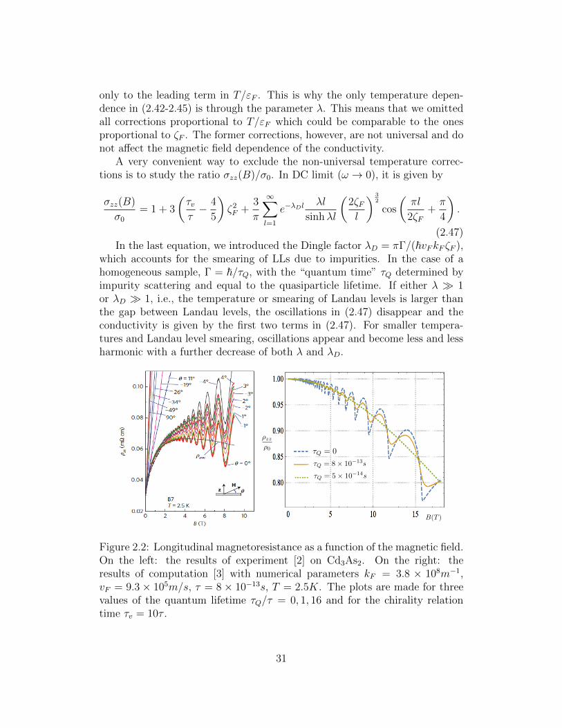
only to the leading term in T/"F . This is why the only temperature depen-dence in (2.42-2.45) is through the parameter �. This means that we omittedall corrections proportional to T/"F which could be comparable to the onesproportional to ⇣F . The former corrections, however, are not universal and donot a↵ect the magnetic field dependence of the conductivity.
A very convenient way to exclude the non-universal temperature correc-tions is to study the ratio �zz(B)/�
0
. In DC limit (! ! 0), it is given by
�zz(B)
�0
= 1 + 3
✓
⌧v⌧
� 4
5
◆
⇣2F +3
⇡
1X
l=1
e��Dl �l
sinh�l
✓
2⇣Fl
◆
32
cos
✓
⇡l
2⇣F+
⇡
4
◆
.
(2.47)In the last equation, we introduced the Dingle factor �D = ⇡�/(~vFkF ⇣F ),
which accounts for the smearing of LLs due to impurities. In the case of ahomogeneous sample, � = ~/⌧Q, with the “quantum time” ⌧Q determined byimpurity scattering and equal to the quasiparticle lifetime. If either � � 1or �D � 1, i.e., the temperature or smearing of Landau levels is larger thanthe gap between Landau levels, the oscillations in (2.47) disappear and theconductivity is given by the first two terms in (2.47). For smaller tempera-tures and Landau level smearing, oscillations appear and become less and lessharmonic with a further decrease of both � and �D.
�Q = 0
�Q = 8 ⇥ 10�13s
�Q = 5 ⇥ 10�14s
⇢zz
⇢0
B(T )
Figure 2.2: Longitudinal magnetoresistance as a function of the magnetic field.On the left: the results of experiment [2] on Cd
3
As2
. On the right: theresults of computation [3] with numerical parameters kF = 3.8 ⇥ 108m�1,vF = 9.3 ⇥ 105m/s, ⌧ = 8 ⇥ 10�13s, T = 2.5K. The plots are made for threevalues of the quantum lifetime ⌧Q/⌧ = 0, 1, 16 and for the chirality relationtime ⌧v = 10⌧ .
31

On the right panel of Fig. 2.2 we have plotted the magnetoresisitivitygiven by the inverse of expression in equation (2.47) for parameters consis-tent with the recent experiment on Cd
3
As2
[2]. Comparison with the exper-imental plot on the left panel shows that the approach to magnetotransportin Dirac semimetals developed here describes qualitatively the emergence ofquantum SdH oscillations and the tendency to negative magnetoresistance atstrong magnetic fields (but still small ⇣F ) observed experimentally in Cd
3
As2
[2]. Unfortunately, the direct comparison with experimental data of [2] is dif-ficult due to the large positive magnetoresistance (MR) typical for Cd
3
As2
.The latter has a very complicated unit cell structure and is prone to variousdefects and the cause of positive MR is still unknown. The more thoroughcomparison of our theory with experimental data requires an explanation ofthe positive magnetoresistance. Magnetic field dependent Coulomb screeningmight be one of the reasons for positive MR (see, e.g., [38]) as well as the influ-ence of Zeeman e↵ects on band structure and possible spatial inhomogeneityof samples. On the other hand, our the computation shows a good qualitativeagreement with the data from TaP [4], vide Fig. 2.3.
b)a)
Figure 2.3: Magnetoresistence in TaP, the plot in a) was extracted from [4],whereas the plot in b) was taken from [5].
A much weaker positive MR has also been observed in the weak magneticfield region in Dirac semimetals ZrTe
5
and Na3
Bi and it is believed to be dueto the weak antilocalization.
32

Chapter 3
Hydrodynamics with GaugeAnomaly
The goal of this chapter is to develop variational and Hamiltonian formula-tions of the hydrodynamics with gauge anomaly1. Di↵erently from the pre-vious chapter, this one will be more formal, without a direct connection toexperiments. Yet, one may hope to use some of these ideas to model surfacestates in strongly interacting Weyl materials.
The possibility of an universal hydrodynamic description with additionalhydrodynamic terms taking anomalies into account was noticed initially inAdS/CFT systems [39, 40], and then in genuine relativistic hydrodynamic for-mulation in [41], for a particular case of Abelian gauge anomaly. Togetherwith the CME, the constitutive relations obtained in [41] predict the exis-tence of the chiral vortical e↵ect (CVE), where the current acquires a termproportional to the flow vorticity.
The Hamiltonian formalism is appropriate to study wavelike excitationsand instabilities near the fixed point, through the linear analysis of the eigen-modes, and provides the most appropriate framework to study perturbationtheory and symmetries of the system. We will show how the quantum anomalya↵ects the canonical generators of gauge transformations and di↵eomorphismsas well as their semidirect product algebra. Our approach will be entirely3+1 dimensional, providing a minimal generalization of the standard actionprinciple for fluid dynamics to accommodate anomalies.
The variational problem for hydrodynamics with gauge anomaly in 1+1dimensions was successfully developed in [42], however it cannot be triviallygeneralized to 3+1 dimensions. The most successful attempt so far in finding
1The set of equations (1.31-1.34) can be viewed as two copies of a system with gaugeanomaly.
33
an e↵ective action for equations (3.1-3.4) was given in [43], but the obtainedaction contained unphysical hydrodynamic excitations propagating in a fourthauxiliary spatial dimension. All these approaches rely on an e↵ective action forthe Lagrangian specification of fluid variables [44, 45]. On the other hand, theaction principle for non-abelian hydrodynamics was presented in [46], wherethe authors introduced the idea of coarse graining the coadjoint orbit action.A similar approach to fluid dynamics for spinning particles has been recentlydeveloped in [47]. An action that includes anomalies in the standard modelof particle physics within the framework of the coadjoint orbit method wasgiven in [48]. The anomaly structure in the standard model is di↵erent fromwhat is given in (3.1-3.4) and so the e↵ective action for anomalies in [48] isnot immediately applicable to the present problem.
In the next sections, we will use the so-called Clebsch potentials to parametrizethe Eulerian variables and to write down a variational principle that producesthe anomalous hydrodynamic equations at zero temperature. We will restrictourselves to the flat Minkowski spacetime, though the generalization to moregeneral geometric backgrounds is straightforward. Unless otherwise specified,we will use the Cartesian orthonormal frame, where the pseudo-metric can bechosen as g�⌫ = diag(�1, 1, 1, 1).
The variational principle and the symmetries are analyzed in sections 3.2and 3.3. Using the obtained action, we will derive the corresponding Hamil-tonian formulation specifying the form of the relativistic Hamiltonian and thePoisson brackets. We will emphasize the symmetries of the system and theirmanifestations in Hamiltonian formalism, pointing out the special feature ofone of the Clebsch potentials appearing separately and not via the combina-tion in the dynamic velocity field. This feature is commented on in section3.6. This chapter refers to the work [6]. In the following sections, we will usethe covariant notation and we will set ~ = c = 1 for simplicity.
3.1 Constitutive Relations
Let us start with equations of anomalous hydrodynamics of [41]. The currentand energy-momentum conservation laws for anomalous QFT in the back-ground gauge field can be written as:
@�j� = �C
8✏�⌫�⌧F�⌫F�⌧ , (3.1)
@�T�⌫ = F ⌫�j� . (3.2)
The right hand side of the equation (3.2) is the Lorentz force, while the
34

right hand side of (3.1) is the gauge anomaly term, fully characterized by asingle dimensionless constant C. Here and in the following we will drop theangular brackets denoting expectation values, e.g., hji ! j, so that j� and T �⌫
are classical fields representing the current and the energy-momentum tensor.Assuming local equilibrium and imposing the local form of the second law
of thermodynamics, the authors in [41] were able to constrain the form ofconstitutive relations. In this chapter we are interested in the case of zerotemperature and absence of dissipation. Thus, we will use a particular formof these constitutive relations, which is given by:
j� = nu� +C
12✏�⌫�⌧ µu⌫ (2µ @�u⌧ + 3F�⌧ ) , (3.3)
T �⌫ = nµu�u⌫ + P (µ) g�⌫ . (3.4)
We have introduced the equation of state of the fluid P (µ) which gives thefluid pressure P as a function of the chemical potential µ. The charge densityin the fluid rest frame is given by n = P 0(µ). The fluid 4-velocity u� satisfiesu�u� = �1 and, therefore, has only three independent components. In thiscase, the zeroth component of the equation (3.2) – the energy conservation –is not independent, but can be viewed as a consequence of the other four equa-tions (3.1) and (3.2). The latter four independent equations fully determinethe evolution of n and three independent components of 4-velocity u�.
Equations (3.1-3.4) constitute the first-order hydrodynamics equations writ-ten in Landau frame. Namely, the constitutive relations (3.3) and (3.4) are firstorder in derivatives and the ambiguity in the definition of 4-velocity is resolvedby defining it as an eigenvector of the energy-momentum tensor. Landau framewas used in [49] and was adopted in [41] to construct the hydrodynamics withgauge anomaly.
3.2 Hydrodynamic Action
The variational principle for perfect relativistic fluid dynamics is well knownand goes back to [50, 51]. The key point in finding a hydrodynamic action is theintroduction of a set of variables appropriate to the canonical framework, theso-called Clebsch potentials. For a review on the Clebsch parametrization andvariational principle for relativistic as well as non-relativistic hydrodynamics,vide section 1.5.
The field content of the hydrodynamic action is given by 4 componentsof the 4-current J� and 3 scalar Clebsch potentials (✓,↵, �) parametrizing
35
dynamic velocity ⇠�:
⇠� = @�✓ + ↵@�� . (3.5)
One of the main results of this work is that the action generating equations(3.1-3.4) is given by:
S = �Z
J� (⇠� � A�) + "(n) � C
6✏�⌫⌘�A� ⇠⌫ @⌘ (⇠� + A�)
�
d4x. (3.6)
Here, "(n) is the proper energy density of the fluid which is assumed to bea known function of the proper charge density n. The latter is given by anabsolute value of the 4-current J� as n ⌘
p
�g�⌫J�J⌫ . The second term onthe right hand side of (3.6) describes the anomaly. Taking C = 0 in (3.6) werecover the action for a relativistic perfect fluid without anomaly [50, 51].
The full set of variational equations is obtained by varying (3.6) overJ�, ✓,↵, �. Let us start with equations of motion for J�:
�S
�J�= � (⇠� � A�) + "0(n)
J�n
= 0 . (3.7)
It is convenient to introduce a complete parametrization of the 4-currentJ� in terms of its absolute value n and its direction given by 4-velocity u� as:
J� ⌘ nu� , u�u� = �1 . (3.8)
Then equation (3.7) can be viewed as a relation between the dynamicvelocity, density and the 4-velocity2:
⇠� � A� = µu� , (3.9)
where the chemical potential µ(n) is given by the derivative of the energydensity as:
µ(n) ⌘ "0(n) . (3.10)
Clebsch potentials ✓,↵, � enter (3.6) only through ⇠� given by (3.5). The
2For the case of irrotational flows, such as superfluids, the dynamic velocity can be fullycharacterized by @�✓ and equation (3.9) corresponds to Josephson condition.
36

corresponding variations give the following equations of motion:
�S
�✓= @�
✓
�S
�⇠�
◆
= 0 , (3.11)
�S
�↵=
�S
�⇠�@�� = 0 , (3.12)
�S
��= @�
✓
↵�S
�⇠�
◆
=�S
�⇠�@�↵ = 0 , (3.13)
with
� �S
�⇠�= nu� +
C
6✏�⌫⌘� [2A⌫@⌘⇠� � (⇠⌫ � A⌫)@⌘A�] . (3.14)
Introducing the charge current:
j� = � �S
�⇠�+
C
6✏�⌫⌘� [3 @⌫(A⌘⇠�) � 3A⌫@⌘A� + ⇠⌫@⌘⇠�] , (3.15)
we obtain (3.1) from (3.11) and (3.5). The relations (3.15) and (3.14) give theconstitutive relation (3.3).
Defining the energy-momentum tensor by (3.4), one can derive the conser-vation law (3.2) from (3.9) and (3.11-3.13) after some tedious but straightfor-ward manipulations3. We will not go through this derivation in more detail,since, in the section 3.3, we will derive equations (3.1-3.4) more straightfor-wardly from symmetries of the action (3.6).
In the absence of the gauge field background A⌫ = 0 the action (3.6)becomes the conventional action for relativistic perfect fluid dynamics [50,51]. The only manifestation of the gauge anomaly in this case is the non-conventional relation between current and 4-velocity. Namely, the relation(3.3) becomes j� = nu� + C
3
µ2!� with relativistic vorticity defined as !� =1
2
✏�⌫�⌧u⌫@�u⌧ . This current is conserved @�j� = 0 because both relations
@�(nu�) = 0 and @�(µ2!�) = 0 follow from (3.6) in the absence of the gaugebackground4 — this consequence can be observed directly from [41] by settingthe temperature and the external fields to zero. Such “removal” of the anomalyresponses by current redefinition is not possible though when a non-trivialgauge field background is present.
3Technical remark: it is convenient to start this derivation with an obvious equation�S�⇠�
⇥
@�
�
�S�J⌫
�
� @⌫
�
�S�J�
�⇤
= 0.4One can think of the second relation as a consequence of (3.1) and (3.2). The second
conserved quantity µ2!� can be identified as a density of the Casimir (helicity) of therelativistic perfect fluid dynamics.
37
3.3 Symmetries
In this section we will show explicitly that the equations (3.1) and (3.2) canbe obtained as consequences of (anomalous) gauge symmetry and space-timetranslational symmetry of the action (3.6), respectively.
The first two terms in (3.6) are symmetric with respect to the gauge trans-formation with the gauge parameter ⇤(x)
�⇤
A� = @�⇤ , �⇤
✓ = ⇤ . (3.16)
From (3.5) and (3.16), we obtain �⇤
⇠� = @�⇤, such that, the combination⇠� � A� in (3.6) is gauge invariant. This gauge invariance, however, is bro-ken by the anomalous part of the action. Up to boundary terms, the gaugetransformation of the action is given by
�⇤
S =
Z
@�⇤
✓
�S
�⇠�+
�S
�A�
◆
d4x =C
6
Z
⇤ ✏�⌫⌘� @�A⌫ @⌘A�d4x. (3.17)
Unlike the case of a general breaking of a symmetry, the loss of symmetrydue to anomalies is rather special. The gauge variation of the action dependsonly on the background gauge field and has a very specific form, the latterbeing determined by the densities of certain topological invariants5. For fieldconfigurations that satisfy the equation of motion (3.11), the variation of (3.17)over ⇤ gives the charge conservation law modulo the anomaly as
@�
✓
�S
�A�
◆
= �C
24✏�⌫�⌧F�⌫F�⌧ . (3.18)
The quantity �S/�A� is known as the consistent current versus the covari-ant current j� defined in (3.3). A quick calculation shows that
j� =�S
�A�
� C
6✏�⌫�⌧A⌫F�⌧ . (3.19)
Taking the divergence of (3.19), we obtain (3.1). We will now turn to theenergy-momentum conservation (3.4). The standard way of deriving this law isto gauge space-time translational symmetries by introducing the background
5It is easy to see that the action can be made fully gauge invariant by supplementing itwith the Chern-Simons term �C
6
R
M5A^dA^dA. The integral in this term is taken over an
auxiliary 5-dimensional space M5 which boundary coincides with the physical space-time.This gives an elegant interpretation of the anomaly of the 4-dimensional theory as beingdue to the inflow of charge from the fifth dimension, a set-up known as anomaly inflow ; thisis standard and well known in QFT with quantum anomalies.
38

metric and study the invariance of the action under di↵eomorphisms x� !x� + ⇣�(x).
Let us consider (3.6) in an arbitrary background metric by replacing themeasure d4x by the invariant one
p�g d4x and by introducing the metricinto all scalar products. Notice that ⇠� is naturally a covariant vector, beingderivatives of the scalar Clebsch potentials, and thus J� ⇠� being an invariantscalar product does not require additional metric factors. However, a scalarproduct like J2 will become JµJ⌫ gµ⌫ . The resulting action is invariant underdi↵eomorphisms, i.e., �⇣S = 0, and on equations of motion we have
Z
(L⇣g)⌫��S
�g⌫�+ (L⇣A)�
�S
�A�
�
d4x = 0 , (3.20)
since the terms corresponding to the variations of the fields vanish by theequations of motion. Here L⇣ denotes the Lie derivative with respect to thevector field ⇣. Explicitly
(L⇣g)⌫� = @⌫⇣� + @�⇣⌫ , (3.21)
(L⇣A)� = ⇣⌫F⌫� + @�(⇣⌫A⌫) . (3.22)
Using these formulas and setting the coe�cient of ⇣⌫ in (3.20) to zero weobtain6
@�T�⌫ = F⌫�
�S
�A�
� C
6F⌫� ✏
�⌘�⌧A⌘F�⌧ , (3.23)
with
T �⌫ ⌘ � 2p�g
�S
�g�⌫, (3.24)
A quick calculation shows that the energy-momentum tensor (3.24) is thesame as (3.4). This is expected since the last term of (3.6) is the integralof a 4-form — which is metric-independent — and gives no contribution tothe energy-momentum tensor. Therefore, (3.4) is identical in form to theenergy-momentum tensor for conventional perfect fluid dynamics. The metricindependence of the anomalous contribution to (3.6) is an essential feature ofthe analysis in the hydrodynamic Landau frame where the energy-momentumtensor is not modified by corrections which are of the first order in gradientsof the velocity.
Finally, it is easy to see that the equation (3.23) with the relation (3.19)is equivalent to (3.2). This completes the demonstration that the action (3.6)does indeed reproduce equations (3.1-3.4).
6The identity A⌫ ✏�⌘�⌧F�⌘F�⌧ = �4F⌫� ✏�⌘�⌧A⌘F�⌧ can be useful.
39

3.4 Hamiltonian Formalism
In this section we will set up the Hamiltonian formulation of equations (3.1-3.4) starting with the action (3.6). Let us start by reducing the 7 independentvariational fields of (3.6) to 4, given by J0 and by the Clebsch parameters✓,↵, �. The spatial components of (3.8) and (3.9) combine to
Ji =n
µ(⇠i � Ai). (3.25)
We can thus eliminate the spatial components of the current J i using (3.25).The definition of n, namely (J0)2 � (J i)2 = n2, gives us
J0 ⌘ ⇢ =n
µ
p
µ2 + (⇠i � Ai)2 . (3.26)
Here and in the following we will use ⇢ to denote J0. We can regard ⇢as the independent variable, with n given implicitly as a function of ⇢ by(3.26)7. Substituting (3.25) and (3.26) into (3.6) we obtain the action which islinear in the time-derivatives and depends only on fields ⇢, ✓,↵, �. After someintegrations by parts, it can be brought to the following form:
S =
Z
⇣
h⇡✓ , ✓i + h⇡� , �i � H⌘
dt , (3.27)
where hf, gi ⌘R
f(x)g(x) d3x denotes the L2-inner product in the space of realfunctions, H is the Hamiltonian, ⇡✓ and ⇡� are the canonical field momentaconjugate to ✓ and �, respectively. The explicit formulas for the canonicalmomenta are:
⇡✓ = �
⇢+C
6(Ai + ↵ @i�)B
i
�
, (3.28)
⇡� = �↵
⇢+C
6(Ai � @i✓)B
i
�
. (3.29)
The Hamiltonian H in (3.27) is given by
H =
Z
h
⇢p
µ2 + (⇠i � Ai)2 � P (µ) � ⇢A0
i
d3x
� C
6
Z
⇥
⇠iBiA
0
+ ✏ijk(@i✓ � Ai) ⇠jEk
⇤
d3x . (3.30)
7As µ(n) is assumed to be a known function of n (3.10) the equation (3.26) can inprinciple be solved to obtain n(⇢, ⇠i), µ(⇢, ⇠i) etc.
40
The pressure P (µ) is related to the energy density by the Legendre trans-form "(n) = nµ�P (µ), with P 0(µ) = n and we have also introduced the mag-netic and electric fields Bi = ✏ijk@jAk and Ei = @iA0
� @0
Ai with ✏ijk ⌘ ✏0ijk.Although the equations of motion (3.1) and (3.4) still do not contain the
Clebsch potentials explicitly, the Hamiltonian (3.30) depends on Clebsch po-tentials not only through ⇠i anymore8. We shall comment on the the meaningof this explicit dependence on ✓ in the following sections. Here we will justpoint out that the coe�cient of Ek in the last term of (3.30) may be inter-preted as an intrinsic fluid electric polarization. It is worth recalling that oneof the main predictions of the anomaly for fluids is the chiral magnetic e↵ectwhich leads to charge separation in a magnetic field. An electric dipole mo-ment obviously suggest a charge separation and we may regard the last termof equation (3.30) as a reflection of this feature in the Hamiltonian framework.
So far we have considered the background gauge field as space and time-dependent. An interesting special case is when the magnetic field is time-independent. It is then possible to choose a vector potential Ai which isindependent of time as well. Then the last term of (3.30) can be integratedby parts and the Hamiltonian takes the form
H =
Z
h
⇢p
µ2 + (⇠i � Ai)2 � P (µ) � A0
⇢i
d3x
� C
6
Z
A0
⇥
2 ⇠iBi + ✏ijk(⇠i � Ai)@j⇠k
⇤
d3x (3.31)
In this case, the explicit dependence on ✓ has disappeared and the Cleb-sch potentials only appear in the combination ⇠i. It is straightforward toobserve that, for a time-independent gauge field, the potential term is simplyR
A0
j0d3x, as one should expect.
3.5 Poisson Brackets
In the this section we will discuss the e↵ect of the anomaly on the Poissonstructure of the Hamiltonian formulation derived in this section. The varia-tional principle (3.27) which is linear in time-derivatives immediately providesus with the canonically conjugate pairs ✓, ⇡✓ and �, ⇡�. The Poisson bracketsof all fields follow then from the canonical ones for the above fields
{✓, ⇡0✓} = {�, ⇡0
�} = �(x � x
0) , (3.32)
8This reduction on equations of motion happens because the Hamiltonian (3.30) is stillinvariant under transformations on the Clebsch potentials which leave ⇠i unchanged.
41

where we have listed only the non-vanishing Poisson brackets. We have useda concise notation omitting the spatial arguments of the fields so that, e.g., �means �(x), ⇡0
✓ means ⇡✓(x0) etc.The hydrodynamic equations of motion (3.1-3.4) can be formulated as
equations written entirely in terms of ⇢ and ⇠i without an explicit dependenceon the Clebsch parameters. Therefore, we shall look for the possible Hamil-tonian reduction of (3.30) and (3.32). The reduction consists of the dynamicreduction, i.e., the Hamiltonian should be expressible only in terms of the den-sity ⇢ and dynamic velocity ⇠i, and the kinematic reduction, i.e., the closureof Poisson brackets of ⇢ and ⇠i without the use of the Clebsch parameters.
As pointed out before, with the inclusion of the anomaly, the dynamicreduction is only partially successful. Namely, the Hamiltonian (3.30) doesdepend on @i✓ in the case of general time-dependent gauge field background.In the case of time-independent background the dynamic reduction is completeand the Hamiltonian (3.31) depends on the Clebsch parameters only through⇠i.
Remarkably, the Poisson algebra of ⇢ and ⇠i is closed for any gauge fieldbackground so that the kinematic reduction is achieved. Indeed, after somestraightforward calculations, we derive from (3.32) and the definition (3.5) thefollowing set of Poisson brackets closed with respect to the fields ⇢ and ⇠i,
�
⇢+
, ⇢0+
=C
3Bi@i �(x � x
0) , (3.33)n
e⇠i, ⇢0+
o
= @i �(x � x
0) , (3.34)
n
e⇠i, e⇠0j
o
= �@ie⇠j � @je⇠i � ✏jikBk
⇢��(x � x
0) . (3.35)
For the sake of brevity, we have introduced the following compact notation,
e⇠i ⌘ ⇠i � Ai , (3.36)
⇢± ⌘ ⇢ ± C
6e⇠i B
i . (3.37)
A comment on the first of these equations, namely (3.33), is appropriateat this point. It is well known that the [j0, j00] commutator will be modi-fied by a Schwinger term in the presence of an anomaly for the correspondingsymmetry. This can be shown by explicit computation of the corrections tocommutators via Feynman diagrams, the triangle diagram leading to the spe-cific form given.9 It can also be seen from a 2-cocycle constructed in terms
9The computation of modified commutators follows a procedure known as the Bjorken-
42

of the descent equations which lead to the anomalies. Our action e↵ectivelyreproduces this in the Poisson brackets. We may also point out that an ex-pression analogous to (3.33) has appeared in [52].
The dynamic velocity e⇠i and the modified densities ⇢± are invariant underthe transformations (3.16), therefore, the Poisson algebra (3.33-3.35) is writ-ten in terms of explicitly gauge-invariant quantities. However, as it is wellknown generator of gauge transformations cannot be realized canonically inthe presence of anomaly (see Sec. 3.6).
The algebra (3.33-3.35) is obtained as a result of Hamiltonian reductionand is degenerate. It admits two Casimirs — the quantities having vanishingPoisson brackets with fields entering Poisson algebra. They are given by
C1
=
Z
⇢+
d3x , (3.38)
C2
=
Z
✏ijk e⇠i @j
⇣
e⇠k + 2Ak
⌘
d3x . (3.39)
The charge density j0 defined in (3.3) is given by
j0 = ⇢+
+C
6✏ijk e⇠i @j
⇣
e⇠k + 2Ak
⌘
. (3.40)
It is a combination of densities of two Casimirs of the algebra. It is worthto point out that when the gauge field is time-independent the anomaly termcan be written as a total derivative, i.e., EiB
i = @i(A0
Bi), what automaticallyimplies that the total charge is indeed conserved.
In the absence of anomaly C = 0, all expressions (3.30, 3.33-3.40) becomethe known formulas for perfect fluid dynamics [46, 53]. Even when the anomalyis present, i.e., C 6= 0, if we consider the case of the background gauge fieldbeing absent, we obtain again the formulas of anomaly-free hydrodynamicswith a single exception. Namely, the definition of the charge density (3.40)still di↵ers from ⇢ by the density of Casimir (3.39). The latter is known as thehelicity of the hydrodynamic flow.
Having Hamiltonian and Poisson brackets, one can obtain equations ofmotion for any quantity Q as Q = @Q/@t + {H,Q}, where @Q/@t denotesthe “explicit” time-derivative. In our case this explicit derivative acts only onthe time varying external gauge field. The dynamical fields ⇠i and ⇢ do notdepend on time explicitly. For example, the equation of motion for ⇠i will reade⇠i = �@tAi + {H, e⇠i}, etc.
Johnson-Low method where correlators of currents at slightly unequal times are calculatedand a suitable equal-time limit is taken.
43

While the Clebsch variables appear in the algebra (3.33-3.35) only via⇠i, we should note that, in the presence of the time-dependent gauge fieldbackground, the Hamiltonian (3.30) contains @i✓ in addition to the densityand the dynamic velocity fields. Thus the algebra (3.33-3.35) is not adequatefor a complete Hamiltonian description, and it should be supplemented byPoisson brackets involving the ✓ field. We will list these brackets here forcompleteness:
{⇢+
, @k✓0} = @k�(x � x
0) , (3.41)
{e⇠i, @k✓0} =e⇠i + Ai � @i✓
⇢�@k�(x � x
0) . (3.42)
3.6 Symmetry generators
The Poisson algebra (3.33-3.35) is closed and, in the case of the time-independentbackground, produces the hydrodynamic equations with the use of the Hamil-tonian (3.31). However, the brackets (3.33-3.35) are nonlinear and thereforedo not have the Lie-Poisson form. For the symmetry analysis it is preferableto find an equivalent set of Poisson brackets corresponding to the algebra ofsymmetry generators of the system.
It is easy to see from (3.27) that the momentum densities can be definedas:
⇥0i = �⇡✓@i✓ � ⇡�@i� . (3.43)
The momentum densities ⇥0i satisfy the di↵eomosphism algebra and act
as local translations in the absence of background field. However, one cannotexpress (3.43) only in terms of the density ⇢ and the dynamic velocity inthe background of nonvanishing magnetic field. More precisely, the canonicalenergy-momentum tensor acquires an explicit ✓ dependence:
⇥0i =
✓
⇢+C
6AkB
k
◆
⇠i +C
6Bk(⇠k@i✓ � ⇠i@k✓) . (3.44)
Let us now turn to gauge transformations which can be viewed as shiftsin the field ✓. The naive canonical gauge generator for this symmetry is �⇡✓.Using (3.28,3.5) we can write it as
� ⇡✓ = ⇢+C
6(Ai + ⇠i � @i✓)B
i (3.45)
and notice that it also depends explicitly on @i✓.It is straightforward to check that the Poisson structure (3.33-3.35) can be
44

put in a semidirect product Lie-Poisson algebra [54] in terms of (3.44) and(3.45). The gauge transformation of an arbitrary functional F of basic fieldsgenerated by �⇡✓ is given by:
�⇤
F ⌘Z
✓
�⇤(x0){⇡0✓, F} +
�F
�Ai(x0)@0i⇤
◆
d3x0 , (3.46)
where the transformation of the gauge potential has also been added.However, it is easy to see that (3.46) gives �
⇤
↵ 6= 0, as well as �⇤
⇢ 6= 0in obvious discrepancy with gauge invariance of ↵ and ⇢. In fact, we willprove by contradiction that the gauge symmetry (3.16) cannot be canonicallyrealizable. Let us assume that there exists a generator Q
⇤
, such that,
{Q⇤
, ✓(x)} = ⇤(x), (3.47)
{Q⇤
,↵(x)} = {Q⇤
, ⇢(x)} = {Q⇤
, �(x)} = 0. (3.48)
From the Jacobi identity, we obtain:
{⇢(x0), {Q⇤
,↵(x)}} � {↵(x), {Q⇤
, ⇢(x0)}} = {Q⇤
, {↵(x), ⇢(x0)}}. (3.49)
The right hand side can be evaluated using equation (C.9):
{Q⇤
, {↵(x), ⇢(x0)}} = �C2
36
Bi@i↵
⇢2�(Bk@k⇤)�(x � x
0). (3.50)
On the other hand, using the definition (3.48), we find that the left handside vanishes, which concludes the proof.
Let us now consider ⇢+
given by (3.37) as a generator of gauge transfor-mations instead of �⇡✓. We easily check that �
⇤
↵ = �⇤
� = 0 and �⇤
✓ ⌘ ⇤.Moreover, under the modified gauge transformations generated by ⇢
+
the den-sity ⇢ transforms as:
�⇤
⇢ = �C
6Bi@i⇤ , (3.51)
and there exists the gauge invariant quantity ⇢+ C6
BiAi.While ⇢
+
can be considered as a modified generator of gauge transforma-tions two subsequent gauge transformations generated by ⇢
+
do not commuteand the commutative algebra of gauge transformations has acquired a cen-tral extension (3.33). This is, of course, a classical manifestation of a wellknown phenomenon in studies of quantum anomalies. At this point it is notclear whether similar modifications can be made for di↵eomorphism generators
45

(3.43)10.
10The variables ↵ and ⇢ do not transform nicely under these generators.
46
Chapter 4
Odd Viscosity from VariationalPrinciple
Odd viscosity e↵ects in incompressible fluids cannot be observed in flat spacewithout the introduction of a boundary. For the compressible case, on theother hand, we can always get rid of the odd viscosity term by some momentumredefinition. It would be convenient to have a frame independent way todefine odd viscosity without such ambiguities. Since the odd viscosity term isdissipationless, one may hope to capture it in the hydrodynamic action. Oncewe have the variational principle, coupling with a geometrical backgrounduniquely defines the momentum density and stress tensor. Thus, we will beable to lift the ambiguity in the odd viscosity definition.
The work presented in this chapter has not been published yet.
4.1 Odd Viscosity Ambiguity
In this section, we will show that, in a compressible fluid with conserved charge,the odd viscosity term (1.47) can be introduced or removed by a momentumredefinition. The possibility of such redefinition is a direct consequence of thecontinuity equation on the density of the conserved charge.
In the case of FQH fluid, the odd viscosity ⌘H is called Hall viscosity 1.4and it is proportional to the average orbital spin per particle [29, 30, 55]. As wewill show in this section, this relation also holds for general two-dimensionalfluids. Let us consider a compressible fluid on the plane with intrinsic angularmomentum. If s is the average spin per particle, the expression for the totalangular momentum can be written as:
L =
Z
d2x�
✏ikxiPk + s⇢�
, (4.1)
47

where Pi is the momentum density. Let us assume for simplicity that totalintrinsic angular momentum of the fluid is extensive, that is, s is a constant.Thus, we can rewrite the equation (4.1) as:
L =
Z
d2x ✏ijxi
⇣
Pj +s
2�jk✏
kl@l⇢⌘
=
Z
d2x ✏ijxi⇧j, (4.2)
where ⇧i is the modified momentum density. Equations (4.1) and (4.2) di↵erby boundary terms. Let us consider for simplicity the system with Galileansymmetry, that is, momentum and current are the same1. As a consequenceof the continuity equation, we find:
@t
⇣
✏ij@j⇢⌘
= �@k
⇣
✏ij@j⇧k + �ij✏kl�lm@j⇧
m⌘
+ @k
⇣
�ik✏jl@j⇧l
⌘
. (4.3)
This identity will play a central role here and in the following section. Toderive the equation (4.3), we have used that @kjk = @kP
k = @k⇧k and that thelast two terms on the right hand side add up to zero. If we define the velocityflow as vi = ⇧i/⇢, equation (4.3) becomes:
@t
⇣
✏ij@j⇢⌘
= �@k
h
⇢ �ij⌘�1
H ⌧ jkH +�
�il✏ljvk + �ji ✏
klvl�
@j⇢ � �ki ✏jl@j(⇢vl)
i
, (4.4)
where ⌧ ikH is the odd viscosity term defined in (1.47), i.e.,
⌧ ikH = ⌘H�
✏ij@jvk + ✏kl�ij@jvl
�
.
Therefore, the addition of 1
2
s �jk✏kl@l⇢ to the perfect fluid momentum den-
sity will automatically introduce the odd viscosity to the system, with:
⌘H =1
2⇢s . (4.5)
Equivalently, if we start with a system with non-vanishing odd viscosityterm, the momentum redefinition:
Pi ! Pi + ��jk✏kl@l⇢,
with always shift the value of the odd viscosity by
⌘H ! ⌘H + �⇢.
From this argument, we obtain that the Hall viscosity is only defined mod-
1This assumption is not necessary though.
48

ulo a real constant times the fluid density. Since � can be associated to theaverage internal angular momentum per fluid particle, we could fix such am-biguity by knowing about the microscopic details of system. In terms of aphenomenological hydrodynamic model, the parameter � can only be deter-mined for a charged fluid. For a charged fluid, the spin density couples to themagnetic field and its e↵ect can be probed through non-uniform configurationsof the external field. However, for a neutral fluid in flat space, the spin densitycan only be obtained by knowing the microscopic detail of the system.
The question we will address throughout this chapter is whether we canlift this ambiguity by fixing � in a phenomenological hydrodynamic model.
4.2 Gradient Corrections to the Perfect FluidAction
In this section, we will formulate the variational principle for the hydrodynam-ics with odd-parity terms. We will show how the ambiguity in the definition ofthe odd viscosity is manifested in this formulation and propose a phenomeno-logical way to resolve this ambiguity. The odd viscosity term in the stresstensor is dissipationless and is of first order in derivative expansion. Let usthus assume that it can be reproduced by adding first order derivative termsin the hydrodynamic action:
S =
Z
h
⇢ ⇠0
+⇢
2�ik⇠i⇠k � "(⇢) + ✏ikf(⇢) @i⇠k
i
dt d2x, (4.6)
where ⇠0
and ⇠i are defined in (3.5), "(⇢) is the internal energy density and f(⇢)is a general function of the particle density ⇢. Di↵erently from the previouschapter, ⇠i now denotes the flow velocity vi and not the dynamic velocity µui.
Notice, that we can add another parity odd term to the hydrodynamicaction:
Z
g(⇢)✏ik⇠i@j⇢ dt d2x.
However, integrating this term by parts, one sees that it only redefines thefunction f(⇢) by:
f(⇢) ! f(⇢) +
Z
g(⇢)d⇢.
49
Equations of motion for the action (4.6) are given by:
✓ : @t⇢+ @i�
⇢⇠i�
= 0 , (4.7)
� : @t↵ +
✓
⇠i +✏ik
⇢@kf
◆
@i↵ = 0 , (4.8)
↵ : @t� +
✓
⇠i +✏ik
⇢@kf
◆
@i� = 0 , (4.9)
⇢ : ⇠0
+⇠i⇠i2
� "0(⇢) + ✏ikf 0(⇢) @i⇠k = 0 . (4.10)
Momentum conservation2 follows from equations (4.7-4.10):
@t (⇢⇠i) = �@k�
⇢⇠k⇠i + �ki P�
, (4.11)
where we have defined the modified pressure P as:
P ⌘ " � ⇢"0 + ⇢f 0✏jl@j⇠l . (4.12)
The expression (4.11) does not have any odd viscosity contribution, butinstead has a parity odd term in the expression for pressure (4.12). As we haveseen in the previous section, by redefining momentum and using the identity(4.3) one can trade the odd contribution to the pressure for odd viscosity.Here we will present a heuristic way to resolve the ambiguity by requiring theodd contribution to the pressure vanish. Let us consider a fluid configurationwith constant density ⇢ = ⇢ slowly rotating as a rigid body with fixed angularvelocity. On one hand the corresponding displacement field does not changeany interparticle distances in a fluid. On the other hand the odd correctionto the pressure is non-vanishing. We argue that this is unnatural and meansthat our definition of the velocity of the fluid (more precisely the relation ofthe velocity with the linear momentum) is incorrect and should be correctedso that the odd term in the pressure disappears.
We can then modify the momentum density in the same way as describedin the last section, i.e.,
⇧i = ⇢⇠i + ��ij✏jk@k⇢.
2In the equation (4.11), we have used the following identity:
✏jk (@if@j⇠k + @jf@k⇠i � @jf@i⇠k) = 0.
.
50

The new momentum density satisfies the following conservation equation:
@t⇧i = �@k
⇧i⇧k
⇢+ �ki P + ⇢�
�
�il✏lj@j⇠
k + ✏kj@i⇠j�
+ O(@2)
�
, (4.13)
whereP = " � ⇢"0 + ⇢(f 0 � �)✏jl@j⇠l . (4.14)
In principle, we can assign any real value to �, given that it cannot be fixedby any symmetry arguments. Therefore, there is a family of stress tensorslabeled by a parameter �. Although in terms of equations all values of �are possible, its value should be fixed by the microscopic theory. The onlyinformation about the microscopic details of the system is encoded into thephenomenological function f(⇢). Using the argument which odd contributionto pressure must vanish at constant density, we obtain:
� = f 0(⇢). (4.15)
And the odd viscosity is given by ⌘H = f(⇢)⇢. It would be ideal to havea more precise mathematical formulation of this argument. In the followingsections, we will show that the knowledge of how the fluid couples to an ex-ternal geometric background (c.f. section 3.3) allows one to fix definitionsof stress and momentum unambiguously. As the considered hydrodynamicsystem is non-relativistic, the proper geometric background is the so-calledNewton-Cartan geometry, which will be discussed in the following section.
4.3 Newton-Cartan Geometry
In this section, we will review the main features of the Newton-Cartan (NC)geometry. For reviews, check [56–58]. We will restrict our discussion to (2+1)-dimensional spacetimes. In Newtonian physics, time and space are separateconcepts, all observers measure the same time. Thus, the non-relativistic orGalilean spacetime is simply given by the cartesian product3 R⇥E2, where R“labels the time” and E2 ⇠= (R2, �) is the Euclidean plane, i.e., the plane R2
endowed with the Euclidean metric �.In complete analogy to the Riemannian geometry, a NC manifold M is
a spacetime that locally resembles the Galilean spacetime R ⇥ E2. In fact,the tangent space TxM at any point x 2 M is isomorphic to R ⇥ E2. Thedevelopment of the NC geometry in (2 + 1) dimensions is out of the scope
3In mathematical jargon, this defines a trivial bundle, where time is base manifold andthe space is the fiber.
51

of this section. Therefore, we will assume some knowledge about di↵erentialgeometry. Let us introduce the set of vielbeins {Eµ
a } and their inverses {eaµ},such that,
Eµa e
bµ = �ba, (4.16)
Eµa e
a⌫ = �µ⌫ . (4.17)
Here, all indices run from 0 to 2 and one can think of Latin indices livingon the tangent space and Greek ones on the spacetime M. The metric struc-ture on each tangent space induces the metric structure on the correspondingpoint on spacetime. Since the tangent-space metric is defined solely to spatialsections, it induces a degenerate metric on M, given by:
�AB eAµ eB⌫ = hµ⌫ . (4.18)
Indices A and B in equation (4.18) label spatial components on TxM andassume only values 1 and 2. The lower-index metric hµ⌫ is degenerate andadmits no inverse. However, we can still define an upper-index metric tensoras:
�ABEµAE
⌫B = hµ⌫ . (4.19)
Since the time direction is special in TxM, let us denote Eµ0
and e0µ by vµ
and nµ respectively. Using the definitions (4.16 - 4.19), we obtain the followingconstraints among NC background fields:
nµvµ = 1, (4.20)
nµhµ⌫ = n⌫h
µ⌫ = 0, (4.21)
vµhµ⌫ = v⌫hµ⌫ = 0, (4.22)
h�µhµ⌫ = �⌫� � n�v
⌫ . (4.23)
Using the symmetry of hµ⌫ and hµ⌫ , we find the total number of geometricalvariables4 to be 18. However, not all of them are independent; in fact, equation(4.23) states for example that hµ⌫ can be expressed in terms of hµ⌫ , vµ andnµ. Out of the 12 components left, equations (4.21) and (4.20) reduces thetotal number of independent ones by 8. This will be important in the nextsection where we will study the invariance of the hydrodynamic action underdi↵eomorphisms.
The spin connection and the a�ne connection are defined by imposing that
4They are 6 from hµ⌫ , 6 from hµ⌫ , 3 from vµ and 3 from nµ.
52

nµ and eAµ are covariantly constant5, that is:
rµeA⌫ ⌘ @µe
A⌫ + �AB✏BC !µe
C⌫ � �
µ⌫ eA = 0, (4.24)
rµn⌫ ⌘ @µn⌫ � �µ⌫n = 0. (4.25)
Notice that in equation (4.24) we have completely stripped o↵ the depen-dence on tangent-space indices from the spin connection, i.e.,
(!µ)AB = �AC✏CB !µ.
Since the spin connection !µ depends only on spacetime indices, it canappear explicitly on the hydrodynamic action as part of the NC geometricalbackground. This is only possible in (2+ 1) dimensions and will be importantin the definition of odd viscosity.
Under local frame rotation the spin connection transforms as:
!µ ! !µ + @µ', (4.26)
where ' is the angle of rotation. The gauge invariant quantity made out fromthe spin connection is curvature 2-form, defined as:
Rµ⌫ = @µ!⌫ � @⌫!µ. (4.27)
The curvature 2-form is related to the Riemann curvature through thefollowing expression:
Rµ⌫ = n✏��h�⌧R
⌧�µ⌫ = n✏
��hµ⌧R⌧⌫��. (4.28)
4.4 Hydrodynamics in Newton-Cartan Back-ground
In section 3.3 we have derived momentum and energy conservations from thegeneral covariance of the the action, that is, �⇣S = 0. However, the action(4.6) is not invariant under general coordinate transformation. Because timeis a special coordinate in Newtonian physics, non-relativistic actions are usu-ally written separating time and spatial coordinates. In order to write them
5In absence of torsion, the a�ne connection can be written as:
�µ⌫⇢ = vµ@⇢n⌫ + 1
2hµ�(@⌫h⇢� + @⇢h⌫� � @�h⌫⇢).
53

covariantly, we need to introduce the NC geometric background discussed inthe previous section. For example, let us focus on the action (4.6). Since ⇠
0
corresponds to the time component of a spacetime one-form, we can rewrite itas the projection of ⇠µ onto a “unit vector” that points towards the directionof time:
⇠0
! vµ⇠µ .
Equivalently, the Euclidean metric and the spatial Levi-Civita tensor mustbe replaced by:
�ik ! hµ⌫ ,
✏ik ⌘ ✏0ik ! nµ✏µ⌫� .
To derive the covariant version of the volume form d2x dt, we must usethat the volume in 3 dimensions can be obtained from the triple product ofthe basis vectors, that is,
d2x dt ! ✏µ⌫� nµe1
⌫e2
� d2x dt.
It is not hard to see that:
✏µ⌫� nµe1
⌫e2
� =q
det (hµ⌫ + nµn⌫). (4.29)
Therefore, the naive covariant version of the action (4.6) can be written as:
S =
Z
M
⇢ vµ⇠µ +1
2⇢hµ⌫⇠µ⇠⌫ � "(⇢) + f(⇢)✏µ⌫� nµ@⌫⇠�
�
dV, (4.30)
where dV ⌘p
det (hµ⌫ + nµn⌫) d2x dt. However, we can always add to the
action (4.30) terms which vanish when we set the NC background to be flat,such as terms proportional to the curvature of M. In fact, there is no uniqueway to make the action (4.6) covariant.
As we pointed out in the previous section, the spin connection can appearexplicitly on the hydrodynamic action. For a flat background we have Rµ⌫ =0, and !µ becomes pure gauge. The gauge transformation (4.26) restrictsthe possible appearance of the spin connection in the action. If the framerotation a↵ects no hydrodynamic variables, !µ can only appear6 in the formRµ⌫ . However, Rµ⌫ can be fully expressed in terms of hµ⌫ , hµ⌫ , vµ and nµ,and the introduction of the !µ in the action is indeed spurious.
6Technically, it could also appear in terms of the formR
✏µ⌫�!µ@⌫a�dV , however theycan be expressed in terms of Rµ⌫ after integration by parts.
54
In analogy to (3.16), let us consider the case where ✓ transform under framerotation:
✓ ! ✓ � s'. (4.31)
We have introduced the constant s, so that the invariant quantity is givenby ⇠µ + s!µ.
4.5 Symmetries in Newton-Cartan Geometry
Here, we will repeat the steps from section 3.3 to derive momentum, energyand spin conservation laws for a non-relativistic 2-dimensional fluid. Let usstart from spin conservation. Since only ✓ and !µ transforms under framerotation:
�'S = �Z
M@�'
✓
s�S
�⇠�� �S
�!�
◆
d2x dt. (4.32)
If we restrict ourselves to field configurations that satisfy equation of mo-tion, we obtain:
@µ
✓
1ph
�S
�!µ
◆
= 0. (4.33)
In the last equation, we have denoted h ⌘ det (hµ⌫ + nµn⌫). Equation(4.33) shows that the spin current is conserved, as a consequence of localframe rotations.
Let us now turn our attention to di↵eomorphisms. As we have alreadydiscussed, not all the NC fields are independent and the variation of hµ⌫ andn⌫ can be expressed in terms of variation of hµ⌫ and vµ:
�nµ = �nµn⌫�v⌫ � 1
2(hµ�n⌫ + h⌫µn�) �h
⌫�, (4.34)
�hµ⌫ = � (h⌫�nµ + hµ�n⌫) �v� � hµh⌫� �h
�. (4.35)
Therefore, on solutions of the equations of motion, the variation of theaction with respect to di↵eomorphisms is given by:
�⇣S =
Z
M
⇢
�S
�vµ� nµn⌫
�S
�n⌫
� (h⌫µn� + hµ�n⌫)�S
�h⌫�
�
(L⇣v)µ +
�S
�!µ
(L⇣!)µ+
�S
�hµ⌫� 1
2(hµ�n⌫ + h⌫�nµ)
�S
�n�
� hµh⌫��S
�h�
�
(L⇣h)µ⌫
�
d2x dt.
(4.36)
55

The Lie derivative L⇣ acting on the background fields gives us:
(L⇣v)µ ⌘ ⇣⌫r⌫v
µ � v⌫r⌫⇣µ = �v⌫r⌫⇣
µ, (4.37)
(L⇣!)µ = ⇣⌫R⌫µ + rµ(⇣⌫!⌫), (4.38)
(L⇣h)µ⌫ = �h⌫�r�⇣
µ � hµ�r�⇣⌫ . (4.39)
Imposing that �⇣S = 0 and using equation (4.33), we find:
Z
M⇣µ✓
r⌫T⌫µ +
1phRµ⌫
�S
�!⌫
◆
dV = 0, (4.40)
where
T ⌫µ =
1ph
✓
v⌫�S
�vµ+ 2h⌫ �S
�hµ� nµ
�S
�n⌫
� 2hµ�S
�h⌫�
◆
. (4.41)
The curvature 2-form appears in the equation for the momentum conser-vation in the same way as the Lorentz force for a charged fluid. However,di↵erently from the latter, the second term in (4.40) can be rewritten as totaldivergence. For that, let us consider the equation (4.28):
1phRµ⌫
�S
�!⌫
= n✏��hµ⌧R
⌧⌫��
1ph
�S
�!⌫
,
1phRµ⌫
�S
�!⌫
= n✏��hµ⌫
h
r� ,r�
i
✓
1ph
�S
�!⌫
◆
. (4.42)
In the last line, we have used the definition of the Riemann tensor. There-fore, equation (4.40) becomes:
r⌫
T ⌫µ + 2n✏
⌫�hµ�r�
✓
1ph
�S
�!�
◆�
= 0. (4.43)
56

Chapter 5
Future Directions: TransportProperties of TopologicalSurface States
The fingerprint of topological materials is the existence of protected surfacestates. In addition to the fundamental interest in states from Fermi arcs,their signature in the magnetotransport appears in small size samples. Forexample, surface modes in the SdH oscillations were observed in [33]. TheFermi arc contribution to quantum oscillations depends on the sample size andwas estimated in [59], using semiclassical arguments. The surface contributionto the conductivity was estimated as:
�� ⇠ cos
2kF
✓
k0
eB
~ cos ✓ + L
◆
± �⇡
�
, (5.1)
where k0
is the Fermi arc length in k-space, � is a phase shift and ✓ is theangle between the magnetic field and the surface normal vector. In additionto that, in very clean samples the states at Fermi arcs may serve as the mainchirality relaxation mechanism.
5.1 Chiral Kinetic Theory with Fermi Arcs
For usual metals, boundary e↵ects are washed out by the bulk properties of thematerials. Therefore, one should expect to see transport signatures of surfacestates only for very thin samples. In this spirit, the Fermi arc contribution forthe SdH oscillations was proposed and estimated in [59]. Their prediction wasqualitatively confirmed later in samples of Cd
3
As2
[33]. To develop a quanti-tative theory of an interplay between bulk anomaly in Weyl/Dirac metals and
57

contributions from surface Fermi arc states the chiral kinetic theory should bemodified by respective boundary terms. This generalized chiral kinetic the-ory with surface states should also account for the chirality relaxation due toFermi arcs.
Our goal is to extend the analysis developed in the chapter 2 to accountfor the surface states discussed in the section 1.2.3. This extension will inhighlight the connection between Fermi arcs and the Atiyah-Patodi-Singerindex theorem, as suggested in [60], and will serve as a basis for the chiralkinetic theory with Fermi arcs.
5.2 Boundary Modes in Anomalous Hydrody-namics
As an alternative approach to kinetic theory we also propose to consider theregime of strong interactions where hydrodynamics can be applicable. The fun-damental question is how to impose realistic boundary conditions on anoma-lous hydrodynamic equations. Due to the topological nature of such surfacestates, we expect that it is possible to impose boundary conditions consistentlyso that the strongly interacting physics corresponding to Fermi arcs would ap-pear as hydrodynamic surface modes derivable from anomalous hydrodynamicsin the bulk with correspondent boundary conditions.
In order to account for surface modes, it is convenient to start from ane↵ective action for anomalous hydrodynamics. In the presence of a boundary,the gauge transformation of the action (3.17) acquires edge contributions:
�⇤
S =C
24
Z
M⇤ ✏�⌫⌘� F�⌫ F⌘� d
4x (5.2)
+C
6
Z
@M⇤ ✏�⌫⌘� (⇠⌫ � A⌫) @⌘ (⇠� + A�) d⌃�.
We notice that the field ✓ appears explicitly in the hydrodynamic actioneven for static (time-independent) background gauge fields. This means thatthis field becomes physical and correspond to physical degrees of freedom ofthe fluid. Therefore, terms containing ⇠i in second line of (5.2) have to becanceled by the gauge variation of a boundary action. This boundary actionhas to be of the form:
S@M =C
6
Z
@M✏�⌫⌘� @⌫✓A⌘ ⇠� d⌃� + gauge invariant terms, (5.3)
58
since
�⇤
(S + S@M) =C
24
Z
M⇤ ✏�⌫⌘� F�⌫ F⌘� d
4x� C
6
Z
@M⇤ ✏�⌫⌘�A⌫@⌘A�d⌃�. (5.4)
The field ✓ becomes physical even for time-independent gauge fields andappears explicitly in the action. Nevertheless, the full action is still invariantto reparametrizations of Clebsch potentials which leave ⇠i invariant.
Let us focus on anomaly terms in the expression for the consistent current:
�S
�A�
= . . .+C
6✏�⌫⌘�
⇠⌫ @⌘⇠� +1
2⇠⌫ F⌘� + @⌫ (A⌘ ⇠�)
�
+ �@M(x)C
6✏�⌫⌘�n⌫ (@⌘✓ � A⌘) ⇠�. (5.5)
In the second line of (5.5), �@M(x) denotes the delta function on the mani-fold boundary. If we compare the consistent charge density, �S/�A
0
, with thelast term in (3.30), we find that the surface charge density is given by thenormal component of the fluid electric polarization.
The extension of this model to two coexistent chiralities and surface hydro-dynamic modes can in principle model the transport in type-I Weyl semimetalswith Fermi arcs. Since the Coulomb interaction breaks the emergent Lorentzsymmetry and hydrodynamic behavior is expected at large temperatures, thenon-relativistic generalization of the e↵ective action for finite temperaturemight become necessary to allow for comparisons with experiments1.
1This is true for e↵ects beyond linear response, where the non-linear nature of hydro-dynamics becomes important.
59

Bibliography
[1] Alexey A. Soluyanov, Dominik Gresch, Zhijun Wang, QuanSheng Wu,Matthias Troyer, Xi Dai, and B. Andrei Bernevig. Type-ii weyl semimet-als. Nature, 527(7579), 2015.
[2] Tian Liang, Quinn Gibson, Mazhar N Ali, Minhao Liu, R J Cava, andN P Ong. Ultrahigh mobility and giant magnetoresistance in the Diracsemimetal Cd3As2. Nature Materials, 14(3):280–284, November 2014.
[3] Gustavo M. Monteiro, Alexander G. Abanov, and Dmitri E. Kharzeev.Magnetotransport in dirac metals: Chiral magnetic e↵ect and quantumoscillations. Phys. Rev. B, 92:165109, Oct 2015.
[4] JianHua Du, HangDong Wang, Qin Chen, QianHui Mao, and et al. Largeunsaturated positive and negative magnetoresistance in weyl semimetaltap. Science China Physics, 2016.
[5] Frank Arnold, Chandra Shekhar, Shu-Chun Wu, Yan Sun, and et al.Negative magnetoresistance without well-defined chirality in the weylsemimetal tap. arXiv:1506.06577, 2015.
[6] Gustavo M. Monteiro, Alexander G Abanov, and V. P. Nair. Hydrody-namics with gauge anomaly: Variational principle and hamiltonian for-mulation. Phys Rev D, 91(125033), 2015.
[7] Bohm-Jung Yang and Naoto Nagaosa. Classification of stable three-dimensional dirac semimetals with nontrivial topology. Nat Commun,5, 2014.
[8] Hongming Weng, Xi Dai, and Zhong Fang. Transition-metal pentatel-luride ZrTe
5
and HfTe5
: A paradigm for large-gap quantum spin hallinsulators. Phys Rev X, 4, 2014.
[9] Qiang Li, Dmitri E. Kharzeev, Cheng Zhang, Yuan Huang, I. Pletikosic,et al. Chiral magnetic e↵ect in zrte
5
. Nature Physics, advance onlinepublication, 02 2016.
60
[10] Sergey Borisenko, Quinn Gibson, Danil Evtushinsky, Volodymyr Zabolot-nyy, Bernd Buchner, and Robert J. Cava. Experimental realization of athree-dimensional dirac semimetal. Phys. Rev. Lett., 113:027603, Jul 2014.
[11] Madhab Neupane, Su-Yang Xu, Raman Sankar, Nasser Alidoust, GuangBian, Chang Liu, Ilya Belopolski, Tay-Rong Chang, Horng-Tay Jeng, HsinLin, et al. Observation of a three-dimensional topological dirac semimetalphase in high-mobility cd3as2. Nature communications, 5, 2014.
[12] Z K Liu, J Jiang, B Zhou, Z J Wang, and et al. A stable three-dimensionaltopological Dirac semimetal Cd
3
As2
. Nature materials, 13, May 2014.
[13] Jun Xiong, Satya Kushwaha, Jason Krizan, Tian Liang, R. J. Cava, andN. P. Ong. Anomalous conductivity tensor in the dirac semimetal na
3
bi.Science, 350(6259), 2015.
[14] B. Q. Lv, H. M. Weng, B. B. Fu, and et al. Experimental discovery ofweyl semimetal taas. Phys Rev X, 5(031013), 2015.
[15] L. X. Yang, Z. K. Liu, Y. Sun, H. Peng, and et al. Weyl semimetal phasein the non-centrosymmetric compound taas. Nat Phys, 11(9), 2015.
[16] N. Xu, H. M. Weng, B. Q. Lv, C. E. Matt, and et al. Observation of weylnodes and fermi arcs in tantalum phosphide. Nat Commun, 7, 2016.
[17] Su-Yang Xu, Nasser Alidoust, Ilya Belopolski, and et al. Discovery of aweyl fermion state with fermi arcs in niobium arsenide. Nat Phys, 11(9),2015.
[18] Su-Yang Xu, Ilya Belopolski, Nasser Alidoust, Madhab Neupane, andet al. Discovery of a weyl fermion semimetal and topological fermi arcs.Science, 349(6248), 2015.
[19] Shin-Ming Huang, Su-Yang Xu, Ilya Belopolski, and et al. A weyl fermionsemimetal with surface fermi arcs in the transition metal monopnictidetaas class. Nat Commun, 6, 2015.
[20] Yuan-Ming Lu Mehdi Kargarian, Mohit Randeria. Are the double fermiarcs of dirac semimetals topologically protected? arXiv:1509.02180, 2015.
[21] Holger Bech Nielsen and Masao Ninomiya. The adler-bell-jackiw anomalyand weyl fermions in a crystal. Physics Letters B, 130(6):389–396, 1983.
[22] Edward Witten. Three lectures on topological phases of matter. Arxivpreprint arXiv: 1510.07698, 2015.
61

[23] Zhijun Wang, Yan Sun, Xing-Qiu Chen, Cesare Franchini, Gang Xu,Hongming Weng, Xi Dai, and Zhong Fang. Dirac semimetal and topolog-ical phase transitions in A
3
bi (a = Na, k, rb). Phys. Rev. B, 85:195320,May 2012.
[24] Zhijun Wang, Hongming Weng, Quansheng Wu, Xi Dai, and Zhong Fang.Three-dimensional dirac semimetal and quantum transport in cd
3
as2
.Phys. Rev. B, 88:125427, Sep 2013.
[25] Kenji Fukushima, Dmitri E Kharzeev, and Harmen J Warringa. Chiralmagnetic e↵ect. Physical Review D, 78(7):074033, 2008.
[26] M Stone. Superfluid dynamics of the fractional quantum hall state. PhysRev B, 42(1):212–217, Jan 1990.
[27] Alexander G Abanov. On the e↵ective hydrodynamics of the fractionalquantum hall e↵ect. Journal of Physics A: Mathematical and Theoretical,46(29):292001, 2013.
[28] J E Avron. Odd viscosity. J Stat Phys, 92(3-4):543–557, Jan 1998.
[29] N Read. Non-abelian adiabatic statistics and hall viscosity in quantumhall states and px+ ipy paired superfluids. Phys Rev B, 79(4):045308, Jan2009.
[30] N Read and E H Rezayi. Hall viscosity, orbital spin, and geometry:Paired superfluids and quantum hall systems. Phys Rev B, 84(8):085316,Jan 2011.
[31] Xiaochun Huang, Lingxiao Zhao, Yujia Long, and et al. Observation of thechiral-anomaly-induced negative magnetoresistance in 3d weyl semimetaltaas. Phys Rev X, 5(031023), 2015.
[32] Zhen Wang, Yi Zheng, Zhixuan Shen, Yunhao Lu, and et al. Helicity-protected ultrahigh mobility weyl fermions in nbp. Phys Rev B,93(121112(R)), 2016.
[33] Philip J. W. Moll, Nityan L. Nair, James G. Analytis, and et al. Chiral-ity transfer dynamics in quantum orbits in the dirac semi-metal cd
3
as2
.arXiv:1505.02817, 2015.
[34] MA Stephanov and Y. Yin. Chiral kinetic theory. Phys Rev Lett, 109,2012.
62

[35] D.T. Son and N. Yamamoto. Berry curvature, triangle anomalies, andchiral magnetic e↵ect in fermi liquids. Phys Rev Lett, 109(181602), 2012.
[36] Ganesh Sundaram and Qian Niu. Wave-packet dynamics in slowlyperturbed crystals: Gradient corrections and berry-phase e↵ects.Phys.Rev.B, 59:14915–14925, 1999.
[37] E. M. Lifshitz, V. B. Berestetski, and L. P. Pitaevskii. Quantum Electro-dynamics. Pergamon, 1982.
[38] J. Klier, I. V. Gornyi, and A. D. Mirlin. Transversal magnetoresistancein weyl semimetals. Phys. Rev. B, 92:205113, Nov 2015.
[39] Johanna Erdmenger, Michael Haack, Matthias Kaminski, and AmosYarom. Fluid dynamics of r-charged black holes. JHEP, 0901:055, 2009.
[40] Nabamita Banerjee, Jyotirmoy Bhattacharya, Sayantani Bhattacharyya,Suvankar Dutta, R. Loganayagam, et al. Hydrodynamics from chargedblack branes. JHEP, 1101:094, 2011.
[41] Dam T Son and Piotr Surowka. Hydrodynamics with triangle anomalies.Phys Rev Lett, 103(19):191601, Jan 2009.
[42] Sergei Dubovsky, Lam Hui, and Alberto Nicolis. E↵ective field theoryfor hydrodynamics: Wess-zumino term and anomalies in two spacetimedimensions. Physical Review D, 89(4):045016, 2014.
[43] FelixM. Haehl, R. Loganayagam, and Mukund Rangamani. E↵ective ac-tions for anomalous hydrodynamics. Journal of High Energy Physics,2014(3), 2014.
[44] Sergei Dubovsky, Lam Hui, Alberto Nicolis, and Dam Thanh Son. E↵ec-tive field theory for hydrodynamics: thermodynamics, and the derivativeexpansion. Physical Review D, 85(8):085029, 2012.
[45] A Nicols and D T Son. Hall viscosity from e↵ective field theory. Arxivpreprint arXiv:1103.2137, Dec 2011.
[46] R Jackiw, V P Nair, S-Y Pi, and A P Polychronakos. Perfect fluid theoryand its extensions. Journal of Physics A: Mathematical and General,37(42):R327, 2004.
[47] Dimitra Karabali and VP Nair. Relativistic particle and relativisticfluids: Magnetic moment and spin-orbit interactions. arXiv preprintarXiv:1406.1551, 2014.
63

[48] VP Nair, Rashmi Ray, and Shubho Roy. Fluids, anomalies, and thechiral magnetic e↵ect: A group-theoretic formulation. Physical ReviewD, 86(2):025012, 2012.
[49] L.D. Landau and E.M. Lifshitz. Fluid mechanics. Course of theoreticalphysics. Butterworth-Heinemann, 1987.
[50] B. F. Schultz. Perfect fluids in general relativity: velocity potential anda variational principle. Phys Rev D, 2, 1970.
[51] B. F. Schultz. Hamiltonian theory of a relativistic perfect fluid. Phys RevD, 4, 1971.
[52] AY Alekseev, VV Cheianov, and J Frohlich. Universality of transportproperties in equilibrium, the goldstone theorem, and chiral anomaly.Phys Rev Lett, 81(16):3503–3506, Jan 1998.
[53] V E Zakharov and EA Kuznetsov. Hamiltonian formalism for nonlinearwaves. Usp Fiz Nauk+, 167(11):1137–1167, Jan 1997.
[54] Darryl D Holm and Boris A Kupershmidt. Relativistic fluid dynamics asa hamiltonian system. Physics Letters A, 101(1):23–26, 1984.
[55] J E Avron, R Seiler, and P G Zograf. Viscosity of quantum hall fluids.Phys Rev Lett, 75(4):697–700, Jan 1995.
[56] Barry Bradlyn and N Read. Low-energy e↵ective theory in the bulk fortransport in a topological phase. arXiv preprint arXiv:1407.2911, 2014.
[57] Andrey Gromov and Alexander G Abanov. Thermal hall e↵ect and ge-ometry with torsion. arXiv preprint arXiv:1407.2908, 2014.
[58] DT Son and M Wingate. General coordinate invariance and conformalinvariance in nonrelativistic physics: Unitary fermi gas. Ann Phys-NewYork, 321(1):197–224, Jan 2006.
[59] Andrew C. Potter, Itamar Kimchi, and Ashvin Vishwanath. Quantumoscillations from surface fermi arcs in weyl and dirac semimetals. NatCommun, 5, 2014.
[60] MA Silaev and GE Volovik. Topological fermi arcs in superfluid 3 he.Physical Review B, 86(21):214511, 2012.
64

Appendix A
Poisson Summation Formulaand SdH E↵ect
In this section, we will apply the Bohr-Sommerfeld quantization prescriptionto introduce quantum e↵ects in the conductivity. Assuming that the onlycontribution to transport comes from the discrete levels, the conductivity perchirality becomes:
�(�)zz = � e2
4⇡2
1X
⌫=�1
Z
dk
1
Z
�1
d(cos ✓) k2
@f0
@"(cos ✓ + �⇣k)
⇥ �[⌫ � 1
4
�
sin2 ✓/⇣k � 2� cos ✓�
]vk gz, (A.1)
where gz is given in (2.40). We have used that there is no real solution for(2.20) when ⌫ 2 Z�. Therefore, all surfaces for negative integer ⌫ are outsideof the integration range. The integral over k is performed near Fermi surface.
Using the Poisson formula,
1X
⌫=�1�(x � ⌫) =
1X
l=�1
ei2⇡l⌫ ,
the conductivity can be rewritten as:
�(�)zz = � e2
4⇡2
1X
l=�1
I(l)1
i! + ⌧�1
v
+I(l)2
i! + ⌧�1
!
, (A.2)
65

where,
I(l)1
=
Z
dk k2v2k@f
0
@"�⇣k e
i⇡l2 (⇣�1
k +⇣k) (A.3)
⇥1
Z
�1
d(cos ✓)(cos ✓ + �⇣k) e�i⇡l
2 (cos ✓+�⇣k)2,
I(l)2
=
Z
dk k2v2k@f
0
@"(1 � ⇣2k) e
i⇡l2 (⇣�1
k +⇣k) (A.4)
⇥1
Z
�1
d(cos ✓)cos ✓ + �⇣k1 + �⇣k cos ✓
cos ✓ e�i⇡l2 (cos ✓+�⇣k)
2.
The integral in equation (A.3) accounts for the intervalley scattering andcan be easily calculated:
I(l)1
= �✓
2
~vFk2
F ⇣2
F
◆
�l,0 . (A.5)
In the equation above, we have used that
@f0
@"⇡ ��(k � kF )
~vF.
The terms with l 6= 0 vanish since the chirality relaxation mechanism thatwe have considered only accounts for the scattering between the zero-modes.
Let us now consider the contribution for the intravalley scattering comingfrom equation (A.4). For l = 0 the integral can be performed analytically,however, we are only interested in the range where the semiclassical picture isvalid. If we restrict ourselves terms up to O(⇣2F ), we end up with:
I(0)
2
= �2
~vFk2
F
1
3� 7
15⇣2F + O(⇣4F )
�
. (A.6)
In order to calculate I(l)2
for l 6= 0, it is convenient to define x = cos ✓+�⇣k.Expanding the integrand up to O(⇣2k), we find that:
I(l)2
=
Z
dk k2 v2k@f
0
@"exp
i⇡l
2(⇣k � 1/⇣k)
�
(A.7)
⇥ [��⇣kQ1
+ (1 + ⇣2k)Q2
� ⇣k�Q3
+ ⇣2kQ4
],
66

where
Qm ⌘1+�⇣kZ
�1+�⇣k
dx xm exp
✓
�i⇡l
2⇣kx2
◆
. (A.8)
Solving for odd values of m:
Q1
=2⇣k⇡l
e�i ⇡l
2⇣k(⇣�1
k +⇣k) sin(⇡l�) = 0,
Q3
=4�i(�1)l⇣2k
⇡le�i⇡l
2 (⇣�1k +⇣k).
However, ⇣kQ3
= O(⇣3k) and such term can be neglected. Let us now focuson m even. They can all be obtained through Q
0
as follows:
Qm =
✓
2i⇣k⇡
◆m/2dm/2
dlm/2Q
0
,
where l is set to be a non-zero integer at the end of the calculation. Clearly,Q
4
= O(⇣3k) and we only need to calculate Q2
. The integral Q0
can be writtenas:
Q0
=
1+�⇣kZ
0
dx e�i ⇡l
2⇣kx2
+
1��⇣kZ
0
dx e�i ⇡l
2⇣kx2
. (A.9)
Let us focus on the right hand side of equation (A.9). Thus,
1±�⇣kZ
0
dx e�i ⇡l
2⇣kx2
=1
2
r
2⇣kil
� 1
2
r
2⇣k⇡l
F0
⇣
⇡l(1±�⇣k)2
2⇣k
⌘
,
where we have defined:
Fm(t) =
Z 1
t
dy y�m�1/2e�iy .
After integration by parts, one can show that:
Fm(t) = �ie�it
tm+1/2+ i
✓
m+1
2
◆
Fm+1
(t).
67
Since we are restricting ourselves to terms up to O(⇣2k), we obtain:
Q0
=
r
2⇣kil
+2⇣k(�1)l
⇡l
e�i⇡l2 (⇣�1
k +⇣k)
1 � ⇣2k,
Q2
= � ei⇡4
⇡
r
2⇣3kl3
+2⇣k(�1)l
⇡le�i⇡l
2 (⇣�1k +⇣k)
✓
i+2⇣k⇡l
◆
.
Plugging all determined values for Qm into (A.7):
I(l)2
= � 2k2
FvF ⇣F~⇡l ei⇡l
✓
i+2⇣F⇡l
◆
(A.10)
�p2ei
⇡4
~⇡l3/2
Z
d" k2vk⇣3/2k
@f0
@"ei
⇡l2 (⇣�1
k +⇣k) .
Here we have used that we can invert the dispersion relation and write k(").The energy integral is performed at the vicinity of the Fermi surface. Since weassume that T/"F ⌧ 1, all the integrand besides the oscillating exponential isconsider to vary slowly in the temperature range. In addition to that, we mustexpand the exponent near the Fermi energy. Keeping only linear deviations inthe exponent, we are left with:
I(l)2
⇡ �2k2
FvF ⇣F~⇡l ei⇡l
✓
i+2⇣F⇡l
◆
(A.11)
� ei⇡4 (1+2l⇣�1
F )
2~⇡ k2
FvF
✓
2⇣Fl
◆
3/21Z
�1
dte(1+i�l/⇡)t
(et + 1)2.
In the equation (A.11), we have defined t = ("�µ)/T and � = ⇡2T/(~vFkF ⇣F ).The integral can be solved using the residue theorem, and its value is givenby:
1Z
�1
e(1+i�l/⇡)t
(et + 1)2dt =
�l
sinh�l.
Therefore, the conductivity can be expressed as:
�(�)zz = �(0)
zz + 21X
l=1
�(l)zz cos
✓
⇡l
2⇣F+
⇡
4
◆
, (A.12)
68

where
�(0)
zz =n�e
2vF~kF
3⇣2Fi! + ⌧�1
v
+1
i! + ⌧�1
✓
1 � 12
5⇣2F
◆�
, (A.13)
and
�(l)zz =
n�e2vF
~kF1
i! + 1/⌧
3
2⇡
�l
sinh�l
✓
2⇣Fl
◆
3/2
. (A.14)
69
Appendix B
Dingle Factor
In the treatment of quantum oscillations, the Dingle factor in equation (2.47)comes from the smearing of LLs due to impurity scattering. In the previoussection, we assumed that the density of states have sharp peaks at each Landaulevel. However, this is not true in a more realistic scenario. The presence ofimpurities breaks the energy degeneracy of the Landau levels and as a netresult they get smeared by the presence of impurities.
The assumption that kF `2B/(vF ⌧) ⌧ 1, allows us to disregard correctionsto the plane-wave scattering due to the magnetic field1. Within this approxi-mation, the density of states is still isotropic, however, it gets a contributioncoming from the smearing of energy levels, namely:
⌫(⇠) =
Z
BZd3k=
⇥
GR(⇠,k)⇤
,
⌫(⇠) =1
⇡
Z
BZd3k
�(⇠, k)
[⇠ � "(k)]2 + �2(⇠, k). (B.1)
In the limit when � ! 0, we recover the well-know result
⌫(⇠) =
Z
BZd3k �(⇠ � "(k)) =
4⇡k2
~vk
�
�
�
�
"=⇠
.
In fact, the smearing of the energy levels can be introduced by followingreplacement:
�(⇠ � "(k)) ! 1
⇡
�(⇠, k)
[⇠ � "(k)]2 + �2(⇠, k).
1Otherwise, we must consider the whole matrix elements of the impurity potential inthe presence of magnetic field.
70

We can thus rewrite equation (A.10) in a more convenient way:
I(l)2
= �2k2
FvF ⇣F~⇡l (�1)l
✓
i+2⇣F⇡l
◆
�p2ei
⇡4
⇡l3/2(B.2)
⇥Z
d⇠
1Z
1p2`B
dk �(⇠ � "(k)) k2v2k ⇣3/2k
@f0
@⇠ei
⇡l2 (⇣�1
k +⇣k) .
The choice of the lower limit of integration is for later convenience. Aspreviously mentioned, the smearing can be taken into account by replacing thedelta function in the integral above by a Lorentzian distribution. Therefore,let us focus on:
Sl(⇠) =1
⇡
1Z
1p2`B
dk�(⇠, k) ei
⇡l2 (⇣�1
k +⇣k)
[⇠ � "(k)]2 + �2(⇠, k)k2v2k⇣
3/2k . (B.3)
The cuto↵ 1/(p2`B) guarantees the integral convergence. One can solve
equation (B.3) using the steepest descent approximation. For that, let us
analytically continue the integrand and define z ⌘ ⇣�1/2k . Hence,
Sl(⇠) =1p8⇡`3B
1Z
1
dz H⇣
⇠, zp2`B
⌘ ei⇡l2 (z2+1/z2)
z,
where
H(⇠, k) ⌘ �(⇠, k) v2k[⇠ � "(k)]2 + �2(⇠, k)
.
Expanding the exponent near z = 1, we obtain:
Sl(⇠) ⇡ (�1)lp8⇡`3B
H⇣
⇠, 1p2`B
⌘
Z
Cdz ei2⇡l(z�1)
2(B.4)
+ip2`3B
Res"!⇠+i�
"
H⇣
⇠, zp2`B
⌘ ei⇡l2 (z2+1/z2)
z
#
.
The contour C is defined by <[(z � 1)2] = 0 together with =[(z � 1)2] � 0and |z| � 1. Let us assume for simplicity that �(⇠, k) = �(⇠). Using that only
71

⇠ ⇠ µ contributes to I(l)2
, we find that:
Sl(⇠) ⇡ (�1)lv20
8⇡`3Bp2l
�
⇠2+
k2vk⇣3/2k
~ exp
✓
i⇡l
2⇣k
◆
, (B.5)
wherev0
⌘ vk|k= 1p2`B
,
and k is taken to be k(⇠ + i�). Plugging it into I(l)2
, we end up with:
I(l)2
= �2k2
FvF ⇣F~⇡l (�1)l
✓
i+2⇣F⇡l
◆
+k3
Fv2
0
�⇣3/2F ei⇡4
⇡2l2"2F
� ei ⇡l2⇣F
+i⇡4��Dl
2~⇡ k2
FvF
✓
2⇣Fl
◆
3/21Z
�1
dte(1+i�l/⇡)t
(et + 1)2.
Here, we have defined �D = ⇡�/(~kFvF ⇣F ) and neglected terms of O(�e��Dl).However, from (2.30),
�/"F ⇠ �/(~vFkF ) ⌧ ⇣F
and consequently ⇣3/2F �/" ⌧ ⇣2F . Therefore, the second term in I(l)
2
can alsobe neglected within our approximation.
The only modification in the conductivity expression coming from thesmearing of LLs occurs in equation (B.6), which must be replaced by:
�(l)zz =
n�e2vF
~kFe��Dl
i! + 1/⌧
3
2⇡
�l
sinh�l
✓
2⇣Fl
◆
3/2
. (B.6)
72

Appendix C
Sympletic Form and PoissonStructure
We can think of the space of functions as an infinite dimensional vector spacewhich can be endowed with a metric structure. Let us define the inner productbetween two functions f and g as
hf, gi ⌘Z
R3
f(x)g(x) d3x.
This inner product defines the so-called L2 metric. Clearly, the convergenceof this integral imposes some conditions on f(x) and g(x), although let us notbother about that for now. Under this, we can understand functions the sameway we understand vectors. Thus, let us rewrite the action in a generic form:
S =
Z tf
ti
⇣
h⇡I , �Ii � H
⌘
dt . (C.1)
Variation of the action gives us:
�S =
Z tf
ti
✓
h⇡I , @t��Ii �
⌧
�H
��I, ��I
�◆
dt+
+
Z tf
ti
⌧
�⇡I , �I � �H
�⇡I
�
dt ,
�S = h⇡I ,��Ii|tfti +
Z tf
ti
⌧
�⇡I , �I � �H
�⇡I
�
dt+
�Z tf
ti
⌧
⇡I +�H
��I, ��I
�
dt .
73

The last two terms give the equations of motion in the Hamiltonian formand the first term introduces the sympletic form. When the momentum vari-ables depend only the fields �I and not on their time derivative, we can expressthe sympletic form as an anti-symmetric bilinear map in space of functions.
⌦ =1
2
Z Z
⌦IJ(x, x0)��I(x) ^ ��J(x0) d3x d3x0, (C.2)
⌦IJ(x, x0) =
✓
�⇡I(x)
��J(x0)� �⇡J(x0)
��I(x)
◆
. (C.3)
In our case, the sympletic form becomes diagonal in position space and canbe written as:
⌦ = �Z
R3
↵ �⇢ ^ �� +C
6@i↵Bi �✓ ^ ��
�
d3x+
�Z
R3
�⇢ ^ �✓ +C
6@i�Bi �↵ ^ �✓
�
d3x+
�Z
R3
✓
⇢+C
6(Ai � @i✓)B
i
◆
�↵ ^ �� d3x . (C.4)
Poisson brackets are obtained by inverting the sympletic form (C.4), whatgives us:
{↵(x), ✓(x0)} = � ↵
⇢��3(x � x0) , (C.5)
{↵(x), �(x0)} =1
⇢��3(x � x0) , (C.6)
{⇢(x), ✓(x0)} = � ⇡�
↵⇢��3(x � x0) , (C.7)
{⇢(x), �(x0)} =C @i�Bi
6⇢��3(x � x0) , (C.8)
{⇢(x),↵(x0)} =C @i↵Bi
6⇢��3(x � x0) , (C.9)
where,
⇢� = ⇢ � C
6(⇠i � Ai)B
i . (C.10)
For the time time dependent Hamiltonian, we need to specify Poissonbracket between (⇠i, ⇢, ✓). The hydrodynamical Poisson brackets then become:
74

{⇢(x), ⇢(x0)} = 0 , (C.11)
{⇠i(x), ✓(x0)} =@i✓ � ⇠i
⇢��3(x � x0) , (C.12)
{⇠i(x), ⇠j(x0)} =@i⇠j � @j⇠i
⇢��3(x � x0) , (C.13)
{⇢(x), ✓(x0)} =⇢+ C
6
(Ai � @i✓)Bi
⇢��3(x � x0) , (C.14)
{⇠i(x), ⇢(x0)} =
C
6Bk (@i⇠k � @k⇠i)
⇢�� @i
�
�3(x � x0) . (C.15)
They simplify if we write the Poisson structure in terms of the free chargedensity ⇢
+
= ⇢+ C6
⇠iBi.
{⇢+
(x), ✓(x0)} = �3(x � x0) , (C.16)
{⇠i(x), ⇢+(x0)} = �@i �3(x � x0) , (C.17)
{⇠i(x), ✓(x0)} =@i✓ � ⇠i
⇢��3(x � x0) , (C.18)
{⇢+
(x), ⇢+
(x0)} = �C
3Bi@i �
3(x � x0) , (C.19)
{⇠i(x), ⇠j(x0)} =@i⇠j � @j⇠i
⇢��3(x � x0) . (C.20)
75

Appendix D
Hamiltonian Equations forHydrodynamic with Anomalies
The Hamiltonian (3.31) in terms of ⇢+
and e⇠i reads:
H =
Z
R3
✓
⇢+
� C
6e⇠iB
i
◆
q
µ2 + e⇠ke⇠k � P (µ)
�
d3x +
+
Z
R3
�
⇢+
+C
6
⇣
✏ijke⇠i @je⇠k + 2(e⇠i + Ai)Bi⌘
�
d3x . (D.1)
The last term depends only on the external fields and it gives no contribu-tion to Hamiltonian equations.
The time evolution of ⇢+
is given by:
⇢+
= {H, ⇢+
} ,
⇢+
= �@i
✓
C
3Bi �H
�⇢+
+�H
�e⇠i
◆
,
and for e⇠i:
e⇠i = {H, e⇠i} ,
e⇠i = �@i
✓
�H
�⇢+
◆
+�H
�e⇠j
1
⇢�
⇣
@ie⇠j � @je⇠i + ✏ijkBk⌘
.
76

The variation of Hamiltonian (D.1) provides us:
�H
�e⇠i= J i +
C
6(2�� �µ)Bi +
C
6✏ijk
⇣
2�@je⇠k + e⇠jEk
⌘
,
�H
�⇢+
= �+ �µ ,
where J i is defined in (??) and,
Ek = �@k�,
�µ =
q
µ2 + e⇠ie⇠i.
The free charge conservation is given by:
⇢+
+ @i
J i +C
6
⇣
�µBi � ✏ijke⇠jEk
⌘
�
=2
3CEiB
i , (D.2)
where we reproduce (3.11). The relativistic Euler equation in the presence ofanomalies becomes:
e⇠i = � vk@ke⇠i � 1
⇢@iP + Ei + ✏ijkv
jBk +C
6
µ�
⇢�✏ijk⇥
⇥ ✏jlm @le⇠m Bk +C
6⇢�
⇣
e⇠lBl vj � ✏jlm e⇠lEm
⌘
⇥
⇥⇣
@ie⇠j � @je⇠i + ✏ijkBk⌘
. (D.3)
77