Annual net community production in the subtropicalPacific Ocean from in situ oxygen measurementson profiling floatsBo Yang1 , Steven R. Emerson1 , and Seth M. Bushinsky2

1School of Oceanography, University of Washington, Seattle, Washington, USA, 2Atmospheric and Oceanic Sciences,Princeton University, Princeton, New Jersey, USA

Abstract Annual net community production (ANCP) in the subtropical Pacific Ocean was determined byusing annual oxygen measurements from Argo profiling floats with an upper water column oxygen massbalance model. ANCP was determined to be from 2.0 to 2.4 mol C m�2 yr�1 in the western subtropical NorthPacific, 2.4 mol C m�2 yr�1 in the eastern subtropical North Pacific, and near zero in the subtropical SouthPacific. Error analysis with the main sources of uncertainty being the accuracy of oxygen measurements andthe parameterization of bubble fluxes in winter suggested an uncertainty of ~0.3 mol C m�2 yr�1 insubtropical Pacific. The results are in good agreement with previous observations in locations where ANCPhas been determined before. These are the first results from the western subtropical North Pacific andsubtropical South Pacific where ANCP have not been evaluated before. ANCP for the subtropical South Pacificis significantly lower than in all other open ocean locations where it has been determined by mass balance.Comparison of our observations with net biological carbon export estimated from remote sensing algorithmsindicates that observations from the subtropical North Pacific are higher than the satellite estimates, butthose in the subtropical South Pacific are lower than satellite-determined carbon export.

1. Introduction

Export of organic carbon from the surface ocean to depth, known as the “biological pump,” plays an impor-tant role in global carbon cycle. It helps maintain the pCO2 of the atmosphere by lowering surface-oceanpCO2 and oxygen minimal zones by influencing oxygen consumption in the ocean thermocline [Longhurstand Harrison, 1989; Hofmann and Schellnhuber, 2009; Kwon et al., 2009]. In the upper ocean, at steady stateover an annual cycle, the flux of biologically produced organic matter to the ocean interior is equal to theannual net community production (ANCP).

The metabolite mass balance approach to measure ANCP comprises a wide range of methods by using dif-ferent chemical tracers, including time series measurements of dissolved inorganic carbon drawdown [e.g.,Lee, 2001; Fassbender et al., 2016], nitrate drawdown [e.g., Wong et al., 2002; Plant et al., 2016], O2/N2 ratio[e.g., Emerson et al., 2008], O2/Ar ratio [e.g., Craig and Hayward, 1987; Emerson et al., 1991; Cassar et al.,2015], and carbon isotope mass balance [e.g., Quay et al., 2009]. In the past decade, development of auton-omous sensor platforms like the gliders and Argo floats made it possible to perform long-term monitoring ofchemical tracers like O2 and nitrate [e.g., Bushinsky and Emerson, 2015; Nicholson et al., 2008; Plant et al., 2016;Riser and Johnson, 2008], which avoids the traditional extrapolation uncertainties from using the summer-only data and allows more accurate estimate of ANCP.

Global estimates of ANCP have been obtained mainly by using two methods: global circulation models[e.g., Bopp et al., 2001] and satellite-based remote sensing observations [e.g., Siegel et al., 2014;Westberry et al., 2012]. However, both model and remote sensing approaches still rely on the field datafor model/algorithm development and for calibration purposes. Emerson [2014] argued that both modeland satellite-determined ANCP are far more geographically variable than experimental measurements.For example, ANCP determined from mass balance at the sites of Hawaii Ocean Time-series (HOT),Ocean Station Papa (OSP), and Bermuda Atlantic Time-series study are 2.5, 2.3, and 3.8 mol C m�2 yr�1,respectively, while the remote sensing estimates (vertically generalized productivity model) at those sitesare 1.4, 4.6, and 1.5 mol C m�2 yr�1, respectively. Greater spatial homogeneity is consistent with recentmodeling studies that describe the consequences of variable C:P ratios in plankton [Teng et al., 2014;DeVries and Deutsch, 2014].

YANG ET AL. ANCP IN SUBTROPICAL PACIFIC 728

PUBLICATIONSGlobal Biogeochemical Cycles

RESEARCH ARTICLE10.1002/2016GB005545

Key Points:• Annual net community production(ANCP) measured with air-calibratedoxygen sensor on profiling floats

• Positive ANCP observed in subtropicalNorth Pacific and near-zero ANCPobserved in subtropical South Pacific

• No single satellite algorithm canreproduce the export productionestimated from Argo O2

measurements across the Pacific

Supporting Information:• Supporting Information S1

Correspondence to:B. Yang,byang9@uw.edu

Citation:Yang, B., S. R. Emerson, andS. M. Bushinsky (2017), Annual netcommunity production in the subtropi-cal Pacific Ocean from in situ oxygenmeasurements on profiling floats,Global Biogeochem. Cycles, 31, 728–744,doi:10.1002/2016GB005545.

Received 3 OCT 2016Accepted 28 MAR 2017Accepted article online 31 MAR 2017Published online 27 APR 2017

©2017. American Geophysical Union.All Rights Reserved.

The western subtropical North Pacific and subtropical South Pacific Ocean are oligotrophic regions with verylow surface nutrient concentrations [Garcia et al., 2014] and extremely low carbon export as determined bysatellite maps [e.g., Siegel et al., 2014; Westberry et al., 2012] and ocean global climate models (GCMs) [e.g.,Bopp et al., 2001]. Because ANCP has not been determined experimentally in these extremely oligotrophicregions we deployed three Argo floats in the western subtropical North Pacific (between 17.7–20.2°N and162–164.5°E, to the southeast of Kuroshio Extension) and one float in the subtropical South Pacific (16.5°S,161.1°E) to do this. We have previously shown that it is possible to determine ANCP by using Argo float-derived oxygen measurements at Ocean Station Papa (OSP) [Bushinsky and Emerson, 2015]. The western sub-tropical North Pacific study area is influenced by the seasonal cycle of southeast summer monsoon andnortheast winter monsoon [Tomczak and Godfrey, 1994], suggesting that monsoon-driven physical processesmight bring nutrients into the euphotic zone of this area. The subtropical South Pacific study area, on theother hand, is under weak but steady westerlies with little seasonality [Tomczak and Godfrey, 1994].

2. Methods2.1. Data Acquisition

Oxygen, salinity, and temperature data used for ANCP calculation were obtained from five University ofWashington (UW) Special Oxygen Sensor Argo floats (SOS-Argo) and an Argo float deployed at the HawaiiOcean Time-series (HOT) by the float group at Monterey Bay Aquarium Research Institute (MBARI)(Figure 1). All floats were operated at a cycle interval of ~5 days.

The Special Oxygen Sensor Argo (SOS-Argo) floats used in this study were equipped with Aanderaa oxygenoptodes (Model 4330, Aanderaa Data Instruments AS, Norway) installed on an ~60 cm long pole attached tothe end cap of floats (Figure 1), which avoids the seawater splash during the surface period and allows pureatmospheric pO2measurements for air calibration. For all SOS-Argo floats, the optode oxygen measurementswere calibrated against the air pO2 calculated from optode temperature, National Centers for EnvironmentalPrediction (NCEP) relative humidity, and sea level pressure data products [Bushinsky et al., 2016]. After eachprofile cycle, when the float reached the surface, the optode measured air pO2 every 2 min for 1 h. Optodeair measurements were quality controlled by filtering out data for which the standard deviation of the pO2

measurements over a 10 min period changed by more than 0.2%, air temperature changed by more than1°C over the air measurement period, or sea level atmosphere pressure changed more than 0.1% duringthe air measurement period. The mean of the remaining pO2 air measurements from each air period wasplotted against the time since deployment to obtain a linear regression for optode calibration. Details ofthe optode air calibration technique are presented in Bushinsky et al. [2016]. The data from this study canbe found on our website (https://sites.google.com/a/uw.edu/sosargo/).

Quality-controlled oxygen data for the float at HOT (float F8497) were obtained fromMBARI database (http://www.mbari.org/science/upper-ocean-systems/chemical-sensor-group/floatviz/). Because the MBARI float didnot have the air calibration mechanism, these data were corrected to ship-based oxygen titrations (0–150 m)from the HOT time series cruises by choosing the Argo profiles obtained within 5 days and 300 km of the HOTship-board measurements (http://hahana.soest.hawaii.edu/hot/hot-dogs/interface.html).

N2 data determined in surface waters at OSP and used in this paper to calibrate the bubble portion of the gasexchange model were obtained from a gas tension device (GTD) on the OSP mooring (see Emerson andStump [2010] and Emerson et al. [2008] for an explanation of the methods used to transform pressure andO2 measurements to N2 concentrations). The O2 and N2 data used here are archived at the Carbon DioxideInformation Analysis Center (http://cdiac.ornl.gov/oceans/Moorings/Papa_145W_50N.html). Wind speeddata used to calculate the air-sea gas exchange mass transfer coefficient were obtained from the advancedscatterometer data product (http://apdrc.soest.hawaii.edu/las/v6/). Sea level pressure and relative humidityproducts used to calibrate the oxygen sensors in air were from National Centers for EnvironmentalPrediction (NCEP) reanalysis (http://www.esrl.noaa.gov/psd/data/gridded/).

The satellite-based net primary production (NPP) estimates and the export production to total primaryproduction ratio (NCP/NPP) were used to calculate remote-sensing-based NCP to compare with our fieldobservations. NPP data were from remote sensing data products (http://www.science.oregonstate.edu/ocean.productivity/index.php), using both the Vertically Generalized Production Model (VGPM) [Behrenfeld

Global Biogeochemical Cycles 10.1002/2016GB005545

YANG ET AL. ANCP IN SUBTROPICAL PACIFIC 729

and Falkowski, 1997] and the Carbon-based Production Model (CbPM) [Westberry et al., 2008]. Ancillary dataused for calculation of NPP (e.g., sea surface temperature) can be found from the same site. The NCP/NPPratio (ef-ratio) used was from Laws et al. [2011].

2.2. Upper Water Column Oxygen Mass Balance Model

Calibrated oxygen, temperature, salinity, atmospheric pressure, and wind speed data were used in an upperocean oxygen mass balance model to calculate ANCP. A schematic of the simplified two-layer upper watercolumn oxygenmass balance model used in this study is presented in Figure 2. Horizontal and vertical advec-tions and changes in oxygen supersaturation caused by float drift are assumed to be small compared toair-sea gas exchange, bubble injection, and diapycnal diffusion as demonstrated by Bushinsky and Emerson[2015] in their study of OSP data [Bushinsky and Emerson, 2015] and as explained in the supporting informa-tion. The model used here has just two layers: the upper mixed layer and a deeper layer with the deepestwinter mixed layer depth as its base. We define ANCP as the flux of organic carbon that escapes the upperocean (sum of layers 1 and 2) after completion of the seasonal mixed layer cycle. Organic carbon exportedfrom the shallow summer mixed layer and respired between layers 1 and 2 is not included in ANCP becauseit can be reventilated to the atmosphere in winter [Bushinsky and Emerson, 2015; Körtzinger et al., 2008;Palevsky et al., 2016b].

Oxygen concentration changes in layer 1 are controlled by gas exchange fluxes, which include both theair-sea interface diffusion (FS) and bubble processes (FB), entrainment of waters from layer 2 to the uppermixed layer (FE), and net biological oxygen production (J1).

d h1 O2½ �ð Þdt

¼ FS þ FB þ FE þ J1 mol m�2 d

�1 (1)

Oxygen change in layer 2 is a result of entrainment (FE), diapycnal eddy diffusion across the base of layer 2(FKz), and net biological oxygen production (J2).

d h2 O2½ �ð Þdt

¼ FE þ FKz þ J2 mol m�2 d

�1 (2)

The sum of J1 and J2 is the total net biological oxygen production (equation (3)) in the upper water column.

Figure 1. Tracks of Argo floats (black, red, and blue lines) in the Pacific with a background of satellite-determined carbonexport from January 2015 to January 2016. Float 8497 (track not shown) was deployed near Hawaii Ocean Time-series (HOT)from 2013 to 2015 in the eastern subtropical North Pacific by Ken Johnson and his colleagues from MBARI. All floatsother than F8497 are UW SOS-Argo floats (pictured above) with air-calibrated oxygen sensors. Satellite-based carbonexport was calculated with net primary production (NPP) from CbPM algorithm [Westberry et al., 2008, http://www.science.oregonstate.edu/ocean.productivity/index.php] multiplied by the NCP/NPP ratio compiled by Laws et al. [2011](equation (11)). The triangles mark the locations of HOT and OSP: Ocean Station Papa.

Global Biogeochemical Cycles 10.1002/2016GB005545

YANG ET AL. ANCP IN SUBTROPICAL PACIFIC 730

JNCP ¼ J1 þ J2 mol m�2 d

�1 (3)

Gas exchange between water and air is modeled as the sum of the air-sea interface exchange, FS, and bubbleprocesses, FB. The air-sea interface flux is calculated from equation (4), where ks is the mass transfer coeffi-cient, [O2] is the float-measured oxygen concentration, and [O2]

sat is the oxygen saturation calculated fromfloat-measured temperature (T) and salinity (S) [Garcia and Gordon, 1992].

FS ¼ FS O2½ � � O2½ �sat� �mol m

�2 d�1 (4)

The mass transfer coefficient for air-sea portion of the exchange has been determined by atmospheric eddycorrelation measurements of dimethyl sulfide (DMS) [Goddijn-Murphy et al., 2016] (see section 3.7 for an ela-boration of this term). The bubble injection flux (FB), is assumed to be the sum of two mechanisms: one ofwhich involves bubbles that are small enough to entirely collapse (Fc), and the other, Fp, for larger bubblesthat exchange gas with the surrounding water and then resurface [Fuchs et al., 1987].

FB ¼ Fc þ Fp mol m�2 d

�1 (5)

Fc is modeled as the product of a mass transfer coefficient (kc) times the atmospheric mole fraction ofoxygen (XO2).

Fc ¼ kCXO2 mol m

�2 d�1 (6)

The gas flux across larger bubbles is the product of a second bubble-induced mass transfer coefficient, kp,and the concentration difference between the oxygen concentration at equilibriumwith the enhanced atmo-spheric pressure inside the bubbles, ΔP, that are subducted below the surface.

Fp ¼ �kp 1þ ΔPð Þ O2½ �sat � O2½ �� �mol m

�2 d�1 (7)

In a previous study [Emerson and Bushinsky, 2016] multiple air-sea gas flux parameterizations from differentbubble models were compared with noble gas data and long-term N2 measurements on the OSP mooring.The model from Liang et al. [2013] proved to match the data best and will be used for this study. Details ofthis parameterization are presented in Liang et al. [2013] and Emerson and Bushinsky [2016].

Figure 2. Schematic of upper water column oxygen mass balance model. The first layer is the mixed layer. The base of thesecond layer is defined as the maximum mixed layer depth in winter. Fluxes (F) are from air-sea gas interface exchangeby diffusion (Fs) and bubble processes (FB), entrainment (FE), and diapycnal eddy diffusion (FKz). J1 and J2 are the fluxes dueto net biological production in layers 1 and 2.

Global Biogeochemical Cycles 10.1002/2016GB005545

YANG ET AL. ANCP IN SUBTROPICAL PACIFIC 731

Entrainment of water from below the mixed layer, FE, is calculated as a product of the mixed layer deepeningrate (dh/dt, m d�1) and the vertical O2 concentration difference (Δ[O2]h1) at the base of the mixedlayer (equation (8)).

FE ¼ dhdt

Δ O2½ �h1 mol m�2 d

�1 (8)

When the mixed layer is deepening the sign of the entrainment flux depends on the concentration gradientbetween layers 1 and 2. There is no flux to the mixed layer when the mixed layer shoals.

For this simplified two-layer model, the diapycnal eddy diffusion flux FKz is considered only at the base of thedeeper layer because this is the boundary used to define the ANCP. This flux is a function of diapycnal diffu-sivity coefficient, Kz, and the O2 concentration gradient, d[O2]/dz across the base of layer 2.

FKZ ¼ KZd O2½ �dz

� �h2

mol m�2 d

�1 (9)

All float data (temperature, salinity, and oxygen concentration) were interpolated into a 1 day interval with adepth resolution of 1 m for the annual mass balance calculation. For each time step, the fluxes describedabove were calculated and net biological oxygen production (JNCP) was derived by using equations (1)–(3).The cumulative JNCP over a year is converted to ANCP by using an oxygen carbon ratio of 1.45 [Hedgeset al., 2002]. The time step in this study was set to be 1 day; decreasing the time step did not alter theANCP result.

In this study, the parameterization (kc and kp) of air-sea exchange through bubble process was optimizedbased on our N2 measurements at OSP. The details can be found in section 3.4. An upper limit for the diapyc-nal eddy diffusion coefficient (Kz) was estimated by using measured oxygen gradients at the winter mixedlayer depth and assuming an oxygen utilization rate (OUR) below this depth (see section 3.5 for detail).

An error analysis of the ANCP calculation was performed by using Monte Carlo method. From our previouswork [Bushinsky and Emerson, 2015], the main uncertainties were determined to be the degree of oxygensupersaturation in the mixed layer, Δ[O2]; three gas exchange mass transfer coefficients (kS, kc, and kp); anddiapycnal diffusivity coefficient (Kz). Randomly distributed errors with carefully determined ranges of uncer-tainties were introduced in the model, and 2000 iterations were run for each variation in the coefficients. Thedetails of how uncertainty ranges were determined can be found in sections 3.4–3.6.

3. Results and Discussion3.1. Atmospheric Calibration of SOS-Argo Oxygen Measurements

The air calibration results of SOS-Argo floats are presented in Figure 3. The intercept of regression line is theoffset between optode air measurements and pO2 at time zero, and the slope of the regression line is the driftrate during the deployment. Linear regressions and error estimates are presented in Table 1. The OSP float(F8397) with the longest record of 4 years has a drift rate of �0.36% yr�1. The South Pacific float (F8485)has a drift rate of �0.14% yr�1, over a period of 2.5 years. The three western North Pacific floats (F9294,F9305, and F9306), however, increased in sensitivity with time during the 1.5 year deployment, with drift ratesof 0.28, 0.18, and 0.08% yr�1. The time zero offsets and drift rates were applied to the raw float data forcorrection. The uncertainty of the atmospheric calibration of the oxygen sensors was estimated from theStudent’s t test and the standard error of the mean of the time series measurements (see Table 1). The stan-dard error of the regression line is smallest at the midpoint of the time series and largest at the ends. To beconservative we use the end values, which have standard errors under ±0.1% using a 67% confidence intervaland about ±0.15% using a 95% confidence interval (Table 1). We adopt an uncertainty of ±0.1% for the air-seaoxygen supersaturation, which is the most important measured term in the oxygen mass balance. This valueis consistent with uncertainties used in previous SOS-Argo float oxygen mass balance studies [Bushinsky andEmerson, 2015; Bushinsky et al., 2016]. We shall see in section 3.7 that minimizing the error on the oxygensupersaturation measurement by using air calibration is essential for determining accurate values of ANCP.

Global Biogeochemical Cycles 10.1002/2016GB005545

YANG ET AL. ANCP IN SUBTROPICAL PACIFIC 732

3.2. Calibration of MBARIArgo Measurements

Since the MBARI float (F8497) contin-ued moving away from HOT, therewere just 11 pairs of Winkler andfloat-derived oxygen data in the top200m of water column available fromFebruary 2013 to December 2014,with an average offset (float-Winkler)of 3.9% (data not shown). A linear fitto the data yielded the followingequation for correction the Optodedata to titration measurements:[O2]corr = 1.2272 × [O2]optode � 57.58(R2 = 0.96, n = 11). The MBARI float(F8497) continued moving awayfrom HOT (Figure S1, bottom), sowe only choose the data within300 km from HOT for this cali-bration. Details of this calibrationprocedure are presented in thesupporting information.

3.3. Oxygen Supersaturation

The evolution of oxygen supersatu-ration in the upper water column(0–150m) for five floats in subtropicalPacific and subarctic OSP is pre-sented in Figure 4. The solid blackline indicates the mixed layer depth,which is often defined by a densityoffset from the value at 10m by usinga threshold of 0.03 kg m�3 [De BoyerMontégut et al., 2004]. However, tomatch the uniform oxygen concen-tration distribution in the mixed

layer, we use a larger threshold of 0.18 kg m�3 for the subtropical floats (see the supporting informationfor details). The mixed layer depth probably varies on a daily time scale (maybe diurnally); however, for ourpurpose we need the deepest value over the period of the gas exchange residence time of about 1 week.For the three western North Pacific floats (Figures 4a–4c), one eastern North Pacific float (Figure 4d), andthe OSP float in the subarctic North Pacific (Figure 4f), the mixed layer started shoaling/deepening on Apriland November, respectively. Correspondingly, oxygen in the mixed layer was supersaturated from mid-April to November and near saturation or slightly undersaturated for the rest of the year. For the SouthPacific float (Figure 4e), the mixed layer started shoaling/deepening on July and January, respectively.Most of the year oxygen in the mixed layer was near saturation or undersaturated, with the lowest oxygensupersaturation observed from mid-June to mid-September.

3.4. Optimization of Air-Sea Gas Exchange Model for Bubble Process

In order to optimize the gas exchange model for bubble processes (including Fc and Fp), a mixed layernitrogen mass balance calculation was carried out to recreate the nitrogen evolution at OSP from June2012 to June 2013 and compared with the measured surface water nitrogen concentrations from GTDon the OSP mooring. The same model used for oxygen was used for nitrogen (equation (1)) except thatJ = 0. [N2] values below the mixed layer are necessary to calculate the entrainment flux, but the dataare only for the surface waters. Deeper values were set to equal the saturation concentrations

Figure 3. Percentage offset between oxygen sensor pO2 measurement in airand the pO2 calculated from atmospheric pressure and the oxygen molefraction, (pO2

optode � pO2air)/pO2

air × 100% for five SOS-Argo floats. Linearregressions (in blue lines, see detail in Table 2) incorporate all available data;only the period from January 2015 to July 2016 was displayed in theabove figure. The error bars represent the standard deviation around themean for 20–30 measurements during each air measurement period.

Global Biogeochemical Cycles 10.1002/2016GB005545

YANG ET AL. ANCP IN SUBTROPICAL PACIFIC 733

calculated by using salinity and temperature from the Argo float as it has been shown previously thatnitrogen concentrations below the mixed layer are close to saturation [Emerson et al., 1991b]. All termson the right side of equation (1) were calculated to obtain a time rate of change, d[N2]/dt that wasevaluated relative to the measurements. Since we are focusing on the model prediction of bubbleprocesses we chose to compare data and model results from a time period with high winds whenbubble processes were strong (14 December 2012 to 25 March 2013). The values of the bubble masstransfer coefficients, kc and kp (equations (6) and (7) in section 2.2), suggested in the model of Lianget al. [2013] were varied by applying correction factors (β) to the bubble mass transfer coefficients ofthe L13 model: kc = β × kc (L13), kp = β × kp (L13), to obtain the smallest residual between themodeled and measured nitrogen concentrations. Since we could solve for just one variable, weassumed the ratio of kc and kp to be the same as determined from the model of Liang et al. [2013]. Theresults of modeled and measured mixed layer [N2] with different correction factors (β) applied to kc andkp from Liang et al. [2013] are presented in Figure 5 and indicate a best fit (with the smallest residualbetween the modeled and measured nitrogen concentrations) of β = 0.53. We adopt this value as thebest estimates for kc and kp for our NCP calculation. In the Monte Carlo error analysis, which followslater in the paper, we assume that our N2-calibrated estimate of the bubble mass transfer coefficients isa lower limit and the L13 parameterization is the upper limit, resulting in an uncertainty of ±25% forthese terms.

3.5. Estimate of Diapycnal Eddy Diffusion Coefficient and Its Uncertainty

The value of the diapycnal eddy diffusion coefficient, Kz, at the base of the winter mixed layer is difficult todetermine because it is a depth region where mixing changes from a very large number in the “mixed layer”to a background value of 1 × 10�5 m2 s�1 as measured by tracer release experiments at a depth of about300 m in the pycnocline [e.g., Ledwell et al., 1993]. Detailed microstructure measurements in the top of thepycnocline [Sun et al., 2013] suggest that the transition from very high to backgroundmixing takes place overa depth interval of about 20 m. We estimate an upper limit for the value of Kz at the base of the winter mixedlayer, h2, by taking advantage of the fact that there are a growing number of observations of the rate ofrespiration in the upper thermocline of the ocean and they are in the range of 25 ± 15 μmol O2 kg

�1 yr�1 (seeTable 2). To estimate an upper limit for the diapycnal eddy diffusion coefficient, we assume that vertical mix-ing is themainmechanism of oxygen supply into the upper thermocline from above. This assumptionmay bewrong as isopycnal transport is an important process of thermocline ventilation, but this assumption is con-sistent with the upper limit calculation. If advection or isopycnal mixing is also important, then we will haveoverestimated the diapycnal diffusion coefficient.

Table 1. SOS Argo Float-Derived Oxygen Uncertainty and Drift Estimates From Air Calibrationa

FloatDeployment

DaysNumber ofAir Periods (n)

Student’s t Uncertainty(t(1 � q/100)[n] × sŶ (%))

Accuracy, b(%)

Drift Rate, a(%/yr)95% Conf. 67% Conf.

F8397 1490 134 0.16 0.08 �4.45 ± 0.17 �0.36 ± 0.06F8485 925 117 0.12 0.06 �2.66 ± 0.23 �0.14 ± 0.13F9294 560 102 0.13 0.07 �2.52 ± 0.13 0.28 ± 0.14F9305 545 101 0.12 0.06 �2.17 ± 0.12 0.18 ± 0.14F9306 540 103 0.13 0.07 �1.95 ± 0.14 0.08 ± 0.16

aThe Student’s t confidence interval from tables is t(1� q/100)[n] x sYi, where q is either 95 or 67 and n is the number

of measurements. The standard error is sYi ¼ffiffiffiffiffiffiffiffiffiffiffiffiffiffiffiffiffiffiffiffiffiffiffiffiffiffiffiffiffiffiffiffiffiffiffiffiffiffiffiffiffiffiffiffiffiffiffis2Y�X

1nþ Xi � X

� �2P

Xi � X� �2

" #vuut , where s2Y�X ¼P

Y � Y� �2n� 2

. The linear regression

lines through the air calibration data in Figure 3 are given by Y = ax + b, where Y is the percentage offset between

measured pO2 and the value in air, (pO2optode � pO2

air)/pO2air × 100% and x is the time since deployment.

Uncertainties in Y (in units of ± percent difference between air and water) are presented using the Student’s t distribu-tion for both 95% and 67% confidence intervals as calculated from the equations in the footnotes [Sokal and Rohlf, 1995].Uncertainties in Y are greater at the ends of the lines than in the middle of the time series, and we present only the lar-gest uncertainties to be conservative. The final two columns are the offset in accuracy extrapolated to the time ofdeployment, b, and the slope of the line, or the drift, a, in %/yr.

Global Biogeochemical Cycles 10.1002/2016GB005545

YANG ET AL. ANCP IN SUBTROPICAL PACIFIC 734

At steady state the integrated respiration rate, the oxygen utilization rate (OUR, mol m�3 s�1), over the depthinterval from high to lowmixing (z = h2 and h2 + 20, respectively) is equal to the flux from above (FKz,h2) minusthe flux at the bottom of the region (FKz,h2 + 20):

∫hþ20

hOUR dz ¼ Fkz ;h2 � Fkz ;h2 þ 20

¼ Kz;h2d O2½ �

.dz

h2� Kz;h2 þ 20

d O2½ �.dz

h2 þ 20

mol m�2 s

�1(10)

The respiration rate range 25 ± 15 μmol O2 kg�1 yr�1(see Table 2 for details) is combined with measured

depth gradients of oxygen in equation (10) to determine the Kz,h2 values at the SOS-Argo float locations(Table 2). The calculation yields an upper limit for Kz,h2 of 2.0–6.0 × 10�5 m2 s�1 at six different locations.We used the midpoint of background Kz value (1.0 × 10�5) [Whalen et al., 2012] and the upper limits calcu-lated in Table 2 in the mass balance model. For floats at OSP (F8397) and South Pacific (F8485), the midpointKz values are 1.5 × 10�5 and 2.3 × 10�5 m2 s�1, respectively. For those four floats at HOT and western NorthPacific, the midpoint Kz value is 3.5 × 10�5 m2 s�1. For the error analysis we assume that the uncertainties of

Figure 4. Oxygen supersaturation ΔO2 (%) = ([O2]/[O2]sat � 1) × 100 as a function of depth and time from five SOS-Argofloats in the Pacific Ocean. The solid black line indicates mixed layer depth.

Global Biogeochemical Cycles 10.1002/2016GB005545

YANG ET AL. ANCP IN SUBTROPICAL PACIFIC 735

Kz are the values necessary to span the range between the upper and lower limit values, which results inerrors for Kz of between ±34% and ±71% (Table 2).

3.6. ANCP Calculated From Oxygen Profiles and Upper Water Column Mass Balance Model

Since we use a somewhat different model here than that used in Bushinsky and Emerson [2015] (hereinafterB15) we demonstrate consistency with our previous work on this subject by calculating ANCP with the sameArgo data used in Bushinsky and Emerson [2015] (Table 3A). The model used in B15 has a mixed layer and aseries of 1-meter-thick layers to 150 meters with vertical eddy diffusion between all layers. The vertical eddydiffusion coefficient (Kz) at the base of the mixed layer was determined from heat/salt budget measurementsat OSP [Cronin et al., 2015], and this value decreases with depth as prescribed by Sun et al. [2013]. In contrast,for the simplified two-layer model used in this study (hereinafter Y17) vertical eddy diffusion is consideredonly at the base of the second layer, with a constant value determined by the methods described above(e.g., 1.5 × 10�5 m�2 s�1 at OSP, see section 3.5 and Table 2). With the same ks, kc, and kp parameterizationsand a constant Kz value of 10

�5 m�2 s�1, our analysis yields an ANCP of 0.4 mol C m�2 yr�1, which is identicalto the result from B15 (Table 3A, row 1). We discovered after the publication of Bushinsky and Emerson [2015]

Table 2. Estimate for the Diapycnal Eddy Diffusion Coefficient at the Base of the Winter Mixed Layer and the Uncertainty of This Valuea

Float Locationd O2½ ��

dz

h2

(mol m�4) d O2½ ��dz

h2þ20

(mol m�4)Kz,h2 (m

2 s�1) Kz=1/2(Kz,h2+20 + Kz,h2) (m2 s�1) Kz (Uncertainty)

F8397 OSP 2.1 × 10�3 2.7 × 10�3 2.0 × 10�5 1.5 × 10�5 ± 34%F8485 South Pacific 0.6 × 10�3 0.6 × 10�3 3.5 × 10�5 2.3 × 10�5 ± 56%F8497 HOT 0.3 × 10�3 0.1 × 10�3 6.3 × 10�5 3.7 × 10�5 ± 73%F9294 Western North

Pacific0.3 × 10�3 0.1 × 10�3 5.7 × 10�5 3.3 × 10�5 ± 70%

F9305 0.3 × 10�3 0.2 × 10�3 5.7 × 10�5 3.3 × 10�5 ± 70%F9306 0.3 × 10�3 0.3 × 10�3 6.0 × 10�5 3.5 × 10�5 ± 71%

aThe upper limit, Kz,h2, is derived from equation (10), where the integrated respiration rate, in the 20 m layer below the winter mixed layer depth (h2), ∫h2þ20h2 OUR

dz; is 25 ± 15 μmol O2 kg�1 yr�1. This value is the mean of five separate estimates of AOU divided by the water tracer age in the top of the thermocline from

different areas of the ocean (Sonnerup et al. [2013, 2015], 16 and 9–25 μmol O2 kg�1 yr�1, respectively; Stanley et al. [2012], 15 μmol O2 kg

�1 yr�1; Kadko [2009],60 μmol O2 kg

�1 yr�1; and Jenkins [1998], 30 μmol O2 kg�1 yr�1). Columns 3 and 4 are the measured oxygen gradients at h2 and h2 + 20 m. Kz,h2 (column 5) is

calculated assuming a value for Kz,h2 + 20 = 1 × 10�5 m2 s�1 (see text). The mean Kz values between that calculated at h2 and assumed at h2 + 20 is in column 6,and the estimated uncertainties (column 7) are the ranges between the upper and lower limits.

Figure 5. Modeled and measured mixed layer N2 concentration during the winter of 2012 to 2013 at Ocean Station Papa(OSP). Data are from GTD and O2 measurements [see Bushinsky and Emerson, 2015], and modeled values are from the gasexchange model of Liang et al. [2013] (L13). (a–c) The modeled result with different correction factors (β) applied to thebubble mass transfer coefficients of the L13 model: kc = β × kc (L13), kp = β × kp (L13). The best fit to the data is with thebubble exchange coefficients decreased by about 50%.

Global Biogeochemical Cycles 10.1002/2016GB005545

YANG ET AL. ANCP IN SUBTROPICAL PACIFIC 736

that there was an error in the accuracy and drift correction in calculation of oxygen concentration. Thisresulted in the oxygen concentration at the beginning of the deployment being 0.2% too low and the valueafter 1 year being 0.3% too low. With the corrected oxygen concentrations, ANCP determined with B15 andY17 are 1.1 and 1.2 mol C m�2 yr�1, respectively (Table 3A, row 2). This difference between ANCP values cal-culated from uncorrected and corrected oxygen data illustrates the extreme sensitivity of ANCP to the mea-sured degree of oxygen supersaturation at OSP. ANCP sensitivity to the value used for Kz, on the other hand, isnot very strong given the range of possible values (Table 3A, row 3). Optimizing the bubble parameters in theL13 model by using the measured N2 values at OSP suggests that the model-predicted bubble-inducedsupersaturation is too strong. Making this correction to the L13 bubble model in both the models of B15and Y17 yields the ANCP of 2.4 mol C m�2 yr�1 (Table 3A, row 4). The reason for the increase in ANCP esti-mates is that bubble injection of O2 in winter (when wind speeds are high) makes the same change indO2/dt as net community production. If bubble injection rates are lower, then the NCP estimate is higher,and the ANCP estimate increases. Note that the correction factors (β) are different for different models, butthe resulting effect on ANCP estimate is nearly the same. The reason for this difference is due to the differentmethods of treating vertical mixing below the mixed layer in the N2 models. This result suggests that our cor-rection to the bubble effect is model-dependent. We believe the more detailed approach in B15 is bound tobe more accurate, but we have shown here that it does not affect the calculated values of ANCP.

Overall, the comparisons in Table 3A indicate no significant difference in ANCP estimates using B15 and Y17models and illustrate the importance of accurate measurements of the air-sea pO2 difference and wintertimebubble processes. With the corrected oxygen data the ANCP of 2012–2013 at OSP reported in Bushinsky andEmerson [2015] is corrected from 0.7 to 1.3 mol C m�2 yr�1. Furthermore, by applying the correction of L13bubble coefficients in both B15 and Y17 models, the best estimate of ANCP at OSP from 2012 to 2013 is2.4 mol C m�2 yr�1. The OSP location is probably one of the most sensitive to these processes anywherein the ocean because wintertime oxygen supersaturation is very close to air equilibrium and wind speedsare extremely strong.

Table 3. (A) Comparison of ANCP Calculated at OSP (2012–2013) Using the Same Data From Float F8397 and theModels of Bushinsky and Emerson [2015] (B15) andThat Used Here (Y17), and (B) ANCP in the Pacific Ocean Using Data From the Other Floats Described in This Paper Calculated From the Y17 Model Described Herea

A

O2 data Model Kz (Parameterization) Kc and Kp (Optimization) ANCP (mol C m�2 yr�1)

B15 OSP Heat/Salt Budget 0.7 ± 0.5

Uncorrected B15 10�5 m�2 s�1 – 0.4 ± 0.5Y17 0.4 ± 0.6

Corrected B15 10�5 m�2 s�1 – 1.1 ± 0.5Y17 1.2 ± 0.6

Corrected B15 OSP Heat/Salt Budget – 1.3 ± 0.5Y17 1.5 × 10�5 m�2 s�1 1.4 ± 0.6

Corrected B15 OSP Heat/Salt Budget β = 0.29 2.4 ± 0.5Y17 1.5 × 10�5 m�2 s�1 β = 0.53 2.4 ± 0.6

B

Location Float Year ANCP (mol C m�2 yr�1)

Subarctic North Pacific (OSP) F8397 2015–2016 2.2 ± 0.6

Eastern Subtropical North Pacific (HOT) F8497b 2014–2015 2.4 ± 0.6

F9294 2.2 ± 0.3Western Subtropical North Pacific F9305 2015–2016 2.0 ± 0.3

F9306 2.4 ± 0.3

Subtropical South Pacific F8485 2014–2015 0.6 ± 0.32015–2016 0 ± 0.3

aSee text for detailed explanation of the values in the different rows.bF8497 is a MBARI Argo float without air-calibration mechanism.

Global Biogeochemical Cycles 10.1002/2016GB005545

YANG ET AL. ANCP IN SUBTROPICAL PACIFIC 737

We applied the Y17 model to annual data from six floats in the Pacific Ocean, using the optimized kc andkp values described in section 3.4 and the Kz values described in section 3.5. An example of model outputfor float F9294 in the western subtropical North Pacific for years 2015–2016 is presented in Figure 6. Figure6a shows daily variations of each flux in equations (1)–(3). The three most important flux terms, other thannet biological production, are the interface air-sea gas flux (FS), bubble injection (FB), and the measuredtime rate of change of oxygen (dh[O2]/dt). From mid-January to mid-March, oxygen in the mixed layerwas undersaturated (Figure 6a), causing a positive flux from the atmosphere to the water (Figure 6a). Asthe seasons progressed to summer oxygen became supersaturated due to a temperature-dependentdecrease in solubility and net biological oxygen production. Bubble fluxes were strong during the winterseason, when wind speeds frequently exceeded 10 m s�1 during winter storms (e.g., March and October).The entrainment flux was significant only during a period of rapid change in mixed layer depth (e.g., Mayand November; Figure 4a). Diapycnal eddy diffusion plays a small role in gas flux because of the rather lowKz value and the relatively weak O2 concentration gradient at the depth of the winter mixed layer. Themodel yielded an ANCP of 2.2 mol C m�2 yr�1 (Figure 6b) for the western subtropical North Pacific.

The ANCP determined from data of the six Argo floats in this study are presented in Table 3B. The ANCP atOSP is determined to be 2.2 mol C m�2 yr�1, which is consistent with the results from 2012(2.5 mol C m�2 yr�1) and previous studies (~2.3 mol C m�2 yr�1 [Emerson, 2014]). For the eastern subtropicalNorth Pacific near HOT (F8497), ANCP is 2.4 mol C m�2 yr�1 for years 2014–2015, which is within the range ofprevious studies (1.4–3.1 mol C m�2 yr�1) based on O2 mass balance [Emerson et al., 2008; Emerson et al.,1995; Hamme and Emerson, 2006], carbon isotope [Brix et al., 2006; Keeling et al., 2004; Quay et al., 2009;Quay et al., 2003], and dissolved inorganic carbon drawdown methods [Lee, 2001]. In the western subtropicalNorth Pacific, the data from all three floats andmodel yield an ANCP from 2.0 to 2.4mol Cm�2 yr�1, which arevery similar to what was observed at HOT in the eastern subtropical North Pacific. Overall, the results from thesubtropical North Pacific are consistent with spatial homogeneity of ANCP described by Emerson [2014].However, we found much lower (near-zero) ANCP values in the subtropical South Pacific. The ANCP valuesare 0.6 and 0 mol C m�2 yr�1 for years 2014–2015 and 2015–2016, respectively, indicating near metabolicbalance over the annual cycle. This is the first value for ANCP determined by mass balance methods thathas indicated little or no net carbon production. It is presently based on data from just one SOS-Argo floatbut suggests the extreme oligotrophic nature of the subtropical South Pacific.

Figure 6. Results of model calculation of ANCP for data from float F9294 in western subtropical North Pacific for the year2015. (a) Daily carbon fluxes calculated with upper water column oxygen mass balance model. Notice that the dominantterms other than J are dhO2/dt (this is measured), and the gas exchange fluxes Fs and FB. (b) Cumulative flux (ANCP)derived from daily carbon fluxes. Presented as carbon fluxes using ΔO2/ΔC = 1.45 [Hedges et al., 2002].

Global Biogeochemical Cycles 10.1002/2016GB005545

YANG ET AL. ANCP IN SUBTROPICAL PACIFIC 738

3.7. Error Analysis

The most critical factor in the error calculation is assigning the range of uncertainty for the values andcoefficients used in the calculation. The most important data term in the mass balance is the value ofthe degree of oxygen supersaturation. Our methods for evaluating the oxygen error are presented insection 3.1 and Table 1. We concluded that an uncertainty of ±0.1% was appropriate for the measurementof oxygen supersaturation between the air and water on SOS-Argo floats. For MBARI float F8497 at HOTwithout air-calibration mechanism, the uncertainty was estimated as ±0.3%, by combining the precisionof HOT Winkler measurements (± 0.2% accessed in September 2016, http://hahana.soest.hawaii.edu/hot/methods/oxygen.html) and all other potential uncertainties (± 0.1%) from sensor measurements and drift.We will see in Table 4 that even this very low value is still one of the most important errors. The othermost significant error is in assessing the accuracy of the bubble flux, which is a model-determined value.Section 3.4 and Figure 5 are devoted to determining the accuracy of the bubble mass transfer coefficientsin the model of Liang et al. [2013]. We argue that the bubble terms are overestimated in winter based oncomparison to N2 concentration data and assume an error that is ±25%. We believe that the bubble flux ispresently the most significant uncertainty in the calculation because it has a great effect on the wintertimeresults and the error estimate is presently based on a single comparison with N2 data. The uncertainty indetermining the diapycnal eddy diffusion coefficient is outlined in section 3.5 and Table 2. We estimateduncertainties that vary from ±34% to ±73% for the five areas of our study. For the Monte Carlo analysis weused an average of ±50%.

The only important term in the error analysis that has not been discussed is the uncertainty in the air-sea gastransfer coefficient, ks. We suggest an error of ±10%, which we determined by comparing the three differentparameterizations for the bubble-free gas exchange rate. Goddijn-Murphy et al. [2016] determined ks as afunction of wind speed based on atmospheric eddy correlation fluxes of dimethyl sulfide (DMS), which isso soluble that it is believed to be unaffected by bubbles. Woolf [1997] used the value determined byJähne et al. [1987] in wind tunnel experiments with no visible bubble formation. The third formulation is thatof the NOAA Coupled Ocean Atmosphere Response Experiment model [Fairall et al., 2003] used by Liang et al.[2013] (L13). At the 10 mwind speed (U10) over the ocean of 6–9m s�1, the difference in k660 (ks at a Schmidtnumber of 660) among these models is about from ±7 to 10%. Since annual mean wind speed values are allaround 7 m/s at our subtropical sites, and 8.6 m/s at the subarctic OSP, we use a more conservative ±10% asthe uncertainty of ks.

The Monte Carlo analysis (Table 4) presents the error derived from each of the terms and that estimated fromthe combination of terms. The results indicate that the uncertainties in oxygenmeasurement and bubble fluxare the most important sources of uncertainties in ANCP estimate. In the subtropical Pacific, compared withSOS-Argo floats, the uncertainty in ANCP is significantly higher for Float 8497 (25% versus 15%), due to thehigher uncertainty in oxygen measurements without air-calibration mechanism. With the same Argo dataset (F8397 at OSP, June 2012 to June 2013) used in Bushinsky and Emerson [2015] at OSP the combined uncer-tainty is about ±30% of the estimated ANCP. This relative value is higher than that in the western subtropical

Table 4. Uncertainties for ANCP Calculated by Using Upper Water Column Mass Balance Modela

Parameter Uncertainty (%)

ANCP Uncertainty (mol C m�2 yr�1)

OSPF8397, 2012–2013

Four Subtropical PacificFloats (ExceptF8497), 2015–2016

Hot, F8497(No Air-Calibration), 2014–2015

Δ[O2] ±0.1 (±0.3 forF8497)

±0.2 ±0.2 ±0.6

ks ±10 ±0.15 ±0.15 ±0.15kc and kp ±25 ±0.5 ±0.2 ±0.2Kz ±50 ±0.2 ±0.1 ±0.1Total – ±0.6 ±0.3 ±0.6

aWe considered the four most serious uncertainties (column 1) to be the degree of oxygen supersaturation Δ[O2]; gasexchange mass transfer coefficients for air-sea diffusive exchange, ks; small bubble collapse, kc; large bubble exchange,kp; and the eddy diffusion coefficient at the base of winter mixed layer, Kz. Column 2 lists the uncertainties explained inthe text and other tables. Uncertainties in ANCP for floats in the subarctic Pacific (OSP) and subtropical Pacific deter-mined by the Monte Carlo calculation described in the text are in columns 3–5

Global Biogeochemical Cycles 10.1002/2016GB005545

YANG ET AL. ANCP IN SUBTROPICAL PACIFIC 739

ocean (±15%) because of the large error in the bubble flux at OSP due to the much higher winds in thesubarctic Pacific. The uncertainty in Kz at OSP is also more important because of the steeper gradient ofoxygen at the base of the winter mixed layer. Past estimates of ANCP by oxygen mass balance even wheninert gases are measured to experimentally determine the effect of bubbles have been in the range of±50%, mostly because of uncertainties in the oxygen measurements [Emerson et al., 1991a]. In this studywe have shown that in situ measurements of pO2 with air calibration can bring down the uncertainty inthe air-sea oxygen gradient. The new challenge with SOS-Argo measurements will be to minimize theerror in the calculation of bubble fluxes at high wind speeds.

3.8. Comparison to Satellite-Based ANCP Estimates

We compare the ANCP values determined here with an estimate of the carbon export determined fromsatellite-derived NPP and model-derived NCP/NPP ratios. The most widely used NPP algorithms are theVertically Generalized Production Model (VGPM) and the Carbon Based Production Model (CbPM). VGPM isa “chlorophyll-based” NPP model, for which NPP is a function of chlorophyll, available light, and photosyn-thetic efficiency [Behrenfeld and Falkowski, 1997]. CbPM, on the other hand, is a carbon based NPP model,which relates the satellite estimates of backscattering to phytoplankton carbon biomass [Westberry et al.,2008]. To calculate satellite-derived NCP, NPP determined by the above models is multiplied by the exportproduction to total primary production ratio (ef-ratio) of Laws et al. [2011], which relates the ef-ratio totemperature (T) and NPP (equation (11)).

Figure 7. NCP determined by Argo oxygen measurements (colored square) and remote sensing data (background color). (left) Results using CbPM algorithm.(right) Results using VGPM algorithm. Satellite-based NCP was calculated with net primary production (NPP) from CbPM/VGPM algorithms [Westberry et al.,2008; Behrenfeld and Falkowski, 1997; http://www.science.oregonstate.edu/ocean.productivity/index.php] multiplied by the NCP/NPP ratio compiled by Laws et al.[2011] (equation (11)). (top to bottom) ANCP from January 2015 to January 2016*, NCP from April to September, NCP from October to March*. For the HOT float(F8497) only the 2014–2015 data are available.

Global Biogeochemical Cycles 10.1002/2016GB005545

YANG ET AL. ANCP IN SUBTROPICAL PACIFIC 740

ef ¼ 0:04756 0:78� 0:43T30

� �NPP0:307 (11)

We chose this ef-ratio because it was parameterized based on measurements of total and export productionfrom a wide range of oceanic habitats, including estimates from the uptake of 15N–labeled nitrate (newproduction), nutrient drawdown, oxygen/carbon-based estimates of export production, and particle exportproduction from sediment trap or 234Th measurements.

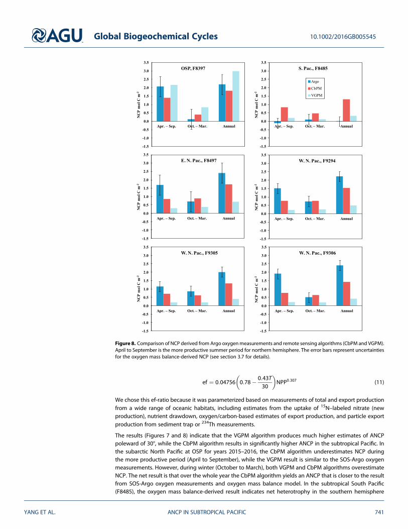
The results (Figures 7 and 8) indicate that the VGPM algorithm produces much higher estimates of ANCPpoleward of 30°, while the CbPM algorithm results in significantly higher ANCP in the subtropical Pacific. Inthe subarctic North Pacific at OSP for years 2015–2016, the CbPM algorithm underestimates NCP duringthe more productive period (April to September), while the VGPM result is similar to the SOS-Argo oxygenmeasurements. However, during winter (October to March), both VGPM and CbPM algorithms overestimateNCP. The net result is that over the whole year the CbPM algorithm yields an ANCP that is closer to the resultfrom SOS-Argo oxygen measurements and oxygen mass balance model. In the subtropical South Pacific(F8485), the oxygen mass balance-derived result indicates net heterotrophy in the southern hemisphere

Figure 8. Comparison of NCP derived from Argo oxygenmeasurements and remote sensing algorithms (CbPM and VGPM).April to September is the more productive summer period for northern hemisphere. The error bars represent uncertaintiesfor the oxygen mass balance-derived NCP (see section 3.7 for details).

Global Biogeochemical Cycles 10.1002/2016GB005545

YANG ET AL. ANCP IN SUBTROPICAL PACIFIC 741

winter (April to September), net autotrophy in the summer (October to March), and overall near zero ANCPfor years 2015 to 2016. The remote sensing products, however, suggest a pattern with positive annual netexport and higher production in the southern hemisphere winter than summer. In this case, the result fromVGPM is closer to oxygen mass balance-derived ANCP. Comparisons of satellite-derived ANCP with data fromthe four floats in the subtropical North Pacific indicate similar seasonal patterns with both oxygen massbalance and remote sensing estimates indicating higher production in the summer. However, the remotesensing estimates of ANCP are always lower than the oxygen mass balance estimates. The CbPMalgorithm-predicted ANCP is closer to the mass balance observations than VGPM.

Overall, assuming the same ef-ratio model of Laws et al. [2011], the ANCP derived from CbPM NPP algorithmis closer to the value derived from the SOS-Argo oxygen data and mass balance model at the subarctic OSPand subtropical North Pacific, while the difference between ANCP-derived from the VGPMNPP algorithm andSOS-Argo oxygenmeasurements is smaller in the subtropical South Pacific. No single-satellite NPP algorithmscan reproduce the export production estimated from Argo oxygen measurements across the Pacific. Thisconclusion is similar to that in the recent comparison made by Palevsky et al. [2016a] for the subtropicalsubarctic boundary. Furthermore, as pointed out by Palevsky et al. [2016a], different choices of ef-ratio willalso affect the result of satellite-based ANCP estimates. Comparisons of satellite-derived and GCM-producedANCP with results of mass balance measurements are still very crude because of the scarcity of experimentalmeasurements and the different definitions of the upper ocean for different approaches. The way forwardwill be to use the comparison between output of GCMs that include ecosystems and metabolite concentra-tions with results of mass balance measurements to derive more accurate distributions of global variations.These values can then be used to tune the remote sensing algorithms. Achieving this goal will require a muchwider distribution of mass balance ANCP measurements.

4. Summary and Conclusions

Continuous oxygen measurements make it possible to determine the flux of biologically produced oxygenout of the upper ocean and infer by stoichiometry the flux of carbon that escapes to the thermocline overthe period of a year: the annual net community production (ANCP). With the oxygen measurements fromArgo profiling floats and an upper water column oxygen mass balance model, ANCP was determined inthe historically undersampled subtropical western North Pacific and South Pacific. In the western subtropicalNorth Pacific, the ~2 mol C m�2 yr�1 estimates of ANCP are the same, within our error, to previous massbalance measurements at eastern North Pacific (HOT). Results from the subtropical South Pacific were deter-mined to be indistinguishable from zero, which is the first value for ANCP from mass balance methods thathave indicated little or no net carbon production.

The largest uncertainties in ANCP calculated from O2 mass balance are from the measurement of the air-seaO2 gradient and the calculation of the gas exchange effect of bubbles in winter. We have been able toimprove the accuracy of the float-measured pO2 difference between the air and the water to a few tenthsof 1% using in situ air calibrations. This improvement reduces the uncertainty of the oxygen mass balanceestimate of ANCP from ±50% [Emerson et al., 1991b] to ± ~30%.

Comparisons with satellite-based ANCP estimates indicated that the oxygen mass balance experimentalresults yielded values higher than satellite estimates in the subtropical North Pacific but lower in the subtro-pical South Pacific. Continuous geochemical tracer measurements like SOS-Argo oxygen measurementspresented here will be necessary to refine both global model and the remote sensing algorithms forpredicting accurate ANCP and biological carbon export over large temporal and spatial scales.

ReferencesBehrenfeld, M. J., and P. G. Falkowski (1997), Photosynthetic rates derived from satellite-based chlorophyll concentration, Limnol. Oceanogr.,

42(1), 1–20.Bopp, L., P. Monfray, O. Aumont, J. L. Dufresne, H. Le Treut, G. Madec, L. Terray, and J. C. Orr (2001), Potential impact of climate change on

marine export production, Global Biogeochem. Cycles, 15(1), 81–99, doi:10.1029/1999GB001256.Brix, H., N. Gruber, D. M. Karl, and N. R. Bates (2006), On the relationships between primary, net community, and export production in sub-

tropical gyres, Deep Sea Res., Part II, 53(5), 698–717.Bushinsky, S. M., and S. Emerson (2015), Marine biological production from in situ oxygen measurements on a profiling float in the subarctic

Pacific Ocean, Global Biogeochem. Cycles, 29, 2050–2060, doi:10.1002/2015GB005251.

Global Biogeochemical Cycles 10.1002/2016GB005545

YANG ET AL. ANCP IN SUBTROPICAL PACIFIC 742

AcknowledgmentsFloat data are available online (https://sites.google.com/a/uw.edu/sosargo/home). Mooring GTD data are availableonline at http://cdiac.ornl.gov/oceans/Moorings/Papa_145W_50N.html.Processed satellite-based NCP data andmodel code are available from theauthors upon request. We thankStephen Riser and Dana Swift for theirassistance in development of the SOS-Argo float, Ken Johnson and his collea-gues from MBARI for permission to usetheir float data at HOT, and scientists ofNOAA Pacific Marine Environmental Lab(PMEL) for hosting the GTD-O2 instru-ment on OSP mooring. This work wassupported by a National ScienceFoundation grant OCE-1458888.

Bushinsky, S. M., S. R. Emerson, S. C. Riser, and D. D. Swift (2016), Accurate oxygen measurements on modified Argo floats using in situ aircalibrations, Limnol. Oceanogr., 14, 491–505, doi:10.1002/lom3.10107.

Craig, H., and T. Hayward (1987), Oxygen supersaturation in the ocean: Biological versus physical contributions, Science, 235(4785), 199–202.Cassar, N., S. W. Wright, P. G. Thomson, T. W. Trull, K. J. Westwood, M. Salas, A. Davidson, I. Pearce, D. M. Davies, and R. J. Matear (2015), The

relation of mixed-layer net community production to phytoplankton community composition in the Southern Ocean, Global Biogeochem.Cycles, 29, 446–462, doi:10.1002/2014GB004936.

Cronin, M. F., N. A. Pelland, S. R. Emerson, and W. R. Crawford (2015), Estimating diffusivity from the mixed layer heat and salt balances in theNorth Pacific, J. Geophys. Res. Oceans, 120, 7346–7362, doi:10.1002/2015JC011010.

de Boyer Montégut, C., G. Madec, A. S. Fischer, A. Lazar, and D. Iudicone (2004), Mixed layer depth over the global ocean: An examination ofprofile data and a profile-based climatology, J. Geophys. Res., 109, C12003, doi:10.1029/2004JC002378.

DeVries, T., and C. Deutsch (2014), Large-scale variations in the stoichiometry of marine organic matter respiration, Nat. Geosci., 7(12),890–894.

Emerson, S. (2014), Annual net community production and the biological carbon flux in the ocean, Global Biogeochem. Cycles, 28, 14–28,doi:10.1002/2013GB004680.

Emerson, S., and S. Bushinsky (2016), The role of bubbles during air-sea gas exchange, J. Geophys. Res. Oceans, 121, 4360–4376, doi:10.1002/2016JC011744.

Emerson, S., and C. Stump (2010), Net biological oxygen production in the ocean—II: Remote in situ measurements of O2 and N2 in subarcticpacific surface waters, Deep Sea Res., Part I, 57(10), 1255–1265.

Emerson, S., P. Quay, C. Stump, D. Wilbur, and M. Knox (1991), O2, Ar, N2, and222

Rn in surface waters of the subarctic ocean: Net biological O2

production, Global Biogeochem. Cycles, 5(1), 49–69, doi:10.1029/90GB02656.Emerson, S., P. Quay, C. Stump, D. Wilbur, and R. Schudlich (1995), Chemical tracers of productivity and respiration in the subtropical Pacific

Ocean, J. Geophys. Res., 100(C8), 15,873–15,887, doi:10.1029/95JC01333.Emerson, S., C. Stump, and D. Nicholson (2008), Net biological oxygen production in the ocean: Remote in situ measurements of O2 and N2 in

surface waters, Global Biogeochem. Cycles, 22, GB3023, doi:10.1029/2007GB003095.Fairall, C. W., E. F. Bradley, J. E. Hare, A. A. Grachev, and J. B. Edson (2003), Bulk parameterization of air–sea fluxes: Updates and verification for

the COARE algorithm, J. Clim., 16(4), 571–591.Fassbender, A. J., C. L. Sabine, and M. F. Cronin (2016), Net community production and calcification from 7 years of NOAA Station Papa

Mooring measurements, Global Biogeochem. Cycles, 30, 250–267, doi:10.1002/2015GB005205.Fuchs, G., W. Roether, and P. Schlosser (1987), Excess

3He in the ocean surface layer, J. Geophys. Res., 92(C6), 6559–6568, doi:10.1029/

JC092iC06p06559.Garcia, H. E., and L. I. Gordon (1992), Oxygen solubility in seawater: Better fitting equations, Limnol. Oceanogr., 37(6), 1307–1312.Garcia, H. E., R. A. Locarnini, T. P. Boyer, J. I. Antonov, O. K. Baranova, M. M. Zweng, J. R. Reagan, and D. R. Johnson (2014), World Ocean Atlas

2013, Volume 4: Dissolved Inorganic Nutrients (Phosphate, Nitrate, Silicate), NOAA Atlas NESDIS, vol. 76, edited by S. Levitus and A. Mishonov,p. 25, U.S. Dep. of Commer., Natl. Oceanic and Atmos. Administr. (NOAA), Natl. Environ. Satell., Data, and Inf. Serv. (NESDIS), Silver Spring, Md.

Goddijn-Murphy, L., D. K. Woolf, A. H. Callaghan, P. D. Nightingale, and J. D. Shutler (2016), A reconciliation of empirical and mechanisticmodels of the air-sea gas transfer velocity, J. Geophys. Res. Oceans, 121, 818–835, doi:10.1002/2015JC011096.

Hamme, R. C., and S. R. Emerson (2006), Constraining bubble dynamics and mixing with dissolved gases: Implications for productivitymeasurements by oxygen mass balance, Journal of Marine Research, 64(1), 73–95.

Hedges, J. I., J. A. Baldock, Y. Gélinas, C. Lee, M. L. Peterson, and S. G. Wakeham (2002), The biochemical and elemental compositions ofmarine plankton: A NMR perspective, Mar. Chem., 78(1), 47–63.

Hofmann, M., and H.-J. Schellnhuber (2009), Oceanic acidification affects marine carbon pump and triggers extended marine oxygen holes,Proc. Natl. Acad. Sci. U.S.A., 106(9), 3017–3022, doi:10.1073/pnas.0813384106.

Jähne, B., K. O. Münnich, R. Bösinger, A. Dutzi, W. Huber, and P. Libner (1987), On the parameters influencing air-water gas exchange, J.Geophys. Res., 92(C2), 1937–1949, doi:10.1029/JC092iC02p01937.

Jenkins, W. J. (1998), Studying subtropical thermocline ventilation and circulation using tritium and3He, J. Geophys. Res., 103(C8),

15,817–15,831, doi:10.1029/98JC00141.Kadko, D. (2009), Rapid oxygen utilization in the ocean twilight zone assessed with the cosmogenic isotope

7Be, Global Biogeochem. Cycles,

23, GB4010, doi:10.1029/2009GB003510.Keeling, C. D., H. Brix, and N. Gruber (2004), Seasonal and long-term dynamics of the upper ocean carbon cycle at Station ALOHA near Hawaii,

Global Biogeochem. Cycles, 18, GB4006, doi:10.1029/2004GB002227.Körtzinger, A., U. Send, R. Lampitt, S. Hartman, D. W. Wallace, J. Karstensen, M. Villagarcia, O. Llinás, and M. DeGrandpre (2008), The seasonal

pCO2 cycle at 49°N/16.5°W in the northeastern Atlantic Ocean and what it tells us about biological productivity, J. Geophys. Res., 113,C04020, doi:10.1029/2007JC004347.

Kwon, E. Y., F. Primeau, and J. L. Sarmiento (2009), The impact of remineralization depth on the air-sea carbon balance, Nat. Geosci., 2(9),630–635, doi:10.1038/ngeo612.

Laws, E. A., E. D’Sa, and P. Naik (2011), Simple equations to estimate ratios of new or export production to total production from satellite-derived estimates of sea surface temperature and primary production, Limnol. Oceanogr.: Methods, 9(12), 593–601.

Ledwell, J. R., A. J. Watson, and C. S. Law (1993), Evidence for slow mixing across the pycnocline from an open-ocean tracer-releaseexperiment, Nature, 364(6439), 701–703.

Lee, K. (2001), Global net community production estimated from the annual cycle of surface water total dissolved inorganic carbon, Limnol.Oceanogr., 46(6), 1287–1297.

Liang, J. H., C. Deutsch, J. C. McWilliams, B. Baschek, P. P. Sullivan, and D. Chiba (2013), Parameterizing bubble-mediated air-sea gas exchangeand its effect on ocean ventilation, Global Biogeochem. Cycles, 27, 894–905, doi:10.1002/gbc.20080.

Longhurst, A. R., and W. G. Harrison (1989), The biological pump: Profiles of plankton production and consumption in the upper ocean, Prog.Oceanogr., 22(1), 47–123.

Nicholson, D., S. Emerson, and C. C. Eriksen (2008), Net community production in the deep euphotic zone of the subtropical North Pacificgyre from glider surveys, Limnol. Oceanogr., 53(5part2), 2226–2236.

Palevsky, H. I., P. D. Quay, and D. P. Nicholson (2016a), Discrepant estimates of primary and export production from satellite algorithms, abiogeochemical model, and geochemical tracer measurements in the North Pacific Ocean, Geophys. Res. Lett., 43, 8645–8653, doi:10.1002/2016GL070226.

Palevsky, H. I., P. D. Quay, D. E. Lockwood, and D. P. Nicholson (2016b), The annual cycle of gross primary production, net communityproduction, and export efficiency across the North Pacific Ocean, Global Biogeochem. Cycles, 30, 361–380, doi:10.1002/2015GB005318.

Global Biogeochemical Cycles 10.1002/2016GB005545

YANG ET AL. ANCP IN SUBTROPICAL PACIFIC 743

Plant, J. N., K. S. Johnson, C. M. Sakamoto, H. W. Jannasch, L. J. Coletti, S. C. Riser, and D. D. Swift (2016), Net community production at OceanStation Papa observed with nitrate and oxygen sensors on profiling floats, Global Biogeochem. Cycles, 30, 859–879, doi:10.1002/2015GB005349.

Quay, P., R. Sonnerup, T. Westby, J. Stutsman, and A. McNichol (2003), Changes in the13C/

12C of dissolved inorganic carbon in the ocean as a

tracer of anthropogenic CO2 uptake, Global Biogeochem. Cycles, 17(1), 1004, doi:10.1029/2001GB001817.Quay, P., J. Stutsman, R. Feely, and L. Juranek (2009), Net community production rates across the subtropical and equatorial Pacific Ocean

estimated from air-sea δ13C disequilibrium, Global Biogeochem. Cycles, 23, GB2006, doi:10.1029/2008GB003193.Riser, S. C., and K. S. Johnson (2008), Net production of oxygen in the subtropical ocean, Nature, 451(7176), 323–325.Siegel, D. A., K. O. Buesseler, S. C. Doney, S. F. Sailley, M. J. Behrenfeld, and P. W. Boyd (2014), Global assessment of ocean carbon export by

combining satellite observations and food-web models, Global Biogeochem. Cycles, 28, 181–196, doi:10.1002/2013GB004743.Sokal, R. R., and F. J. Rohlf (1995) Biometry, 3rd ed., pp. 466–476, W. H. Freeman and Company, Macmillan, New York.Sonnerup, R. E., S. Mecking, and J. L. Bullister (2013), Transit time distributions and oxygen utilization rates in the Northeast Pacific Ocean

from chlorofluorocarbons and sulfur hexafluoride, Deep Sea Res., Part I, 72, 61–71.Sonnerup, R. E., S. Mecking, J. L. Bullister, and M. J. Warner (2015), Transit time distributions and oxygen utilization rates from chlorofluor-

ocarbons and sulfur hexafluoride in the Southeast Pacific Ocean, J. Geophys. Res. Oceans, 120, 3761–3776, doi:10.1002/2015JC010781.Stanley, R. H., S. C. Doney, W. J. Jenkins, and D. E. Lott (2012), Apparent oxygen utilization rates calculated from tritium and helium-3 profiles

at the Bermuda Atlantic Time-series Study site, Biogeosci. Discuss., 8, 9977–10,015.Sun, O. M., S. R. Jayne, K. L. Polzin, B. A. Rahter, and L. C. S. Laurent (2013), Scaling turbulent dissipation in the transition layer, J. Phys.

Oceanogr., 43(11), 2475–2489.Teng, Y. C., F. W. Primeau, J. K. Moore, M. W. Lomas, and A. C. Martiny (2014), Global-scale variations of the ratios of carbon to phosphorus in

exported marine organic matter, Nat. Geosci., 7(12), 895–898.Tomczak, M., and J. S. Godfrey (1994), CHAPTER 8—The Pacific Ocean, in Regional Oceanography, pp. 113–147, Pergamon, Amsterdam.Whalen, C. B., L. D. Talley, and J. A. MacKinnon (2012), Spatial and temporal variability of global ocean mixing inferred from Argo profiles,

Geophys. Res. Lett., 39, L18612, doi:10.1029/2012GL053196.Westberry, T., M. J. Behrenfeld, D. A. Siegel, and E. Boss (2008), Carbon-based primary productivity modeling with vertically resolved

photoacclimation, Global Biogeochem. Cycles, 22, GB2024, doi:10.1029/2007GB003078.Westberry, T. K., P. J. l. B. Williams, and M. J. Behrenfeld (2012), Global net community production and the putative net heterotrophy of the

oligotrophic oceans, Global Biogeochem. Cycles, 26, GB4019, doi:10.1029/2011GB004094.Wong, C., N. A. D. Waser, Y. Nojiri, F. A. Whitney, J. S. Page, and J. Zeng (2002), Seasonal cycles of nutrients and dissolved inorganic carbon at

high and mid latitudes in the North Pacific Ocean during the Skaugran cruises: Determination of new production and nutrient uptakeratios, Deep Sea Res., Part II, 49(24), 5317–5338.

Woolf, D. K. (1997), Bubbles and their role in air-sea gas exchange, in The Sea Surface and Global Change, edited by P. S. Liss and R. A. Duce,pp. 173–205, Cambridge Univ. Press, U. K.

Global Biogeochemical Cycles 10.1002/2016GB005545

YANG ET AL. ANCP IN SUBTROPICAL PACIFIC 744