Embed Size (px)
Citation preview

CPB Discussion Paper
No 45
April, 2005
Financial incentives in Disability Insurance in the
Netherlands
Annemiek van Vuren, Daniel van Vuuren
The responsibility for the contents of this CPB Discussion Paper remains with the author(s)

2
CPB Netherlands Bureau for Economic Policy Analysis
Van Stolkweg 14
P.O. Box 80510
2508 GM The Hague, the Netherlands
Telephone +31 70 338 33 80
Telefax +31 70 338 33 50
Internet www.cpb.nl
ISBN 90-5833-216-0

3
Abstract in English
In this paper, we assess the impact of financial incentives on the inflow in the public Disability
Insurance (DI) scheme in the Netherlands. For this matter, the variation in replacement rates
over different sectors is exploited to estimate the probability of DI enrolment over a sample of
employees from the Dutch Income Panel (1996-2000). On the basis of these administrative
data, we find a point estimate of the elasticity of DI enrolment with respect to the DI wealth rate
of 2.5.
Key words:
Disability Insurance, financial incentives, moral hazard
Abstract in Dutch
In dit paper onderzoeken we het effect van financiële prikkels voor werknemers op de kans dat
zij instromen in de WAO. Vanwege bovenwettelijke afspraken verschillen de financiële
voorwaarden voor deze werknemersverzekering per CAO. Koppeling van deze data aan het
Inkomens Panel Onderzoek (1996-2000) stelt ons in staat om de elasticiteit van de
instroomkans met betrekking tot het ‘WAO-vermogen’ te schatten, wat resulteert in een waarde
van 2,5.
Steekwoorden:
WAO, financiële prikkels, moreel gevaar
Een uitgebreide Nederlandse samenvatting is beschikbaar via www.cpb.nl.

4

5
Contents
Summary 7
1 Introduction 9
2 Institutional setting 13
2.1 A brief history 13
2.2 The current position of Disability Insurance in the Netherlands 14
3 Disability Insurance benefits and individual behaviour 17
4 Data 19
4.1 Replacement rates 19
4.2 Micro data 20
5 Empirical strategy 23
5.1 Incomplete observation 23
5.2 Estimation and testing 26
6 Estimation results 29
7 Conclusion and directions for further research 35
References 37
Appendix A. Replacement rates per sector 41
Appendix B. Parameters and implied elasticities: consistent estimation 43


7
Summary
The number of participants in the Dutch public disability scheme is high in comparison with
other western countries. Several explanations exist for this. First, public disability insurance
(DI) in the Netherlands does not distinguish between occupational risk and social risk, so that
non-work-related disability is also covered by DI. Furthermore, all workers are fully insured
irrespective of their work history, and partially disabled may qualify for disability benefits. A
fourth possible explanation is the relatively high DI replacement rate. In this paper, we try to
find out whether this last factor is a valid explanation for the relatively high use of the public
disability scheme in the Netherlands.
The financial conditions for DI vary for different employees, which is a consequence of the
system of collective labour agreements at the firm or sector level. In this paper, we exploit this
variation over different firms and sectors to identify the effect of financial conditions on the
individual enrolment probability. We find that non-single female workers, older workers (aged
50 to 60 years), and workers in the construction sector face a relatively high risk of DI
enrolment. Younger workers (under 30 years) and workers with young children face a relatively
low risk. Furthermore, we find that a 1% increase in the DI replacement rate implies an increase
in the DI enrolment probability by 2.5%. Suppose for instance that the DI enrolment probability
equals 1% and that the DI replacement rate is raised from 75% to 80% (although these figures
are realistic they do not represent exact figures). Our results then indicate that the DI enrolment
probability will increase to 1.17%. It should be noted that the estimated effect has been
identified on data from the period 1996-2000. It is not unlikely that with the introduction of new
policy measures – such as improvement of the gatekeeper system and the accomplishment of a
system of experience rating – recent years will show a lower elasticity.
In estimating our model, we try to control for the inverse causal effect: it is well possible that a
high risk of becoming disabled implies that workers have a stronger preference for high DI
replacement rates. With the inclusion of amongst others the lagged enrolment probabilities of
firms or sectors we try to control for this. The model we use is the so-called ‘bounded Logit
model’, which is capable of dealing with imperfectly observed enrolment statuses provided that
the actual enrolment probability can be correctly specified by the Logit model. A specification
test indeed shows that our model cannot be rejected.


9
1 Introduction1
In the Netherlands, as well as in many other western countries, the number of participants in
public Disability Insurance (DI) schemes has been growing over the past three decades, which
has led to high expenditures on such schemes and a downward pressure on labour force
participation. Compared to other countries, the use of DI in the Netherlands is relatively high. In
1999 the number of DI enrolments was 10.4 per 1000 insured workers, whereas enrolment in
Germany and the United States equalled 5.3 and 6.0, respectively. In that same year, public
expenditures on DI benefits equalled 2.7% of GDP in the Netherlands, while for Germany and
the US expenditures equalled 1.0% and 0.7%, respectively.2 Several possible explanations may
exist for this difference. Unlike most other countries, DI in the Netherlands does not distinguish
between occupational and social risks, and every worker is fully insured irrespective of his or
her work history. Another difference is that disability is insured from a minimum of 15% of so-
called ‘earnings capacity’, implying that any worker who loses at least 15% of his/her earnings
due to disability will be covered by DI. A fourth reason may be the relatively attractive
financial conditions in the Netherlands (OECD, 2003). The influence of these financial
conditions on DI enrolment is precisely the topic of this paper.
DI schemes are meant to provide insurance against the risk of earnings loss due to disability.
The growth in DI use can however not be explained by an increase of disability within the
population (see, e.g., Aarts en de Jong, 1992). Due to informational problems and imperfect
disability evaluation, able people may receive DI benefits instead of working more hours, or
receive DI benefits instead of unemployment benefits, early retirement benefits, or welfare.
Such improper use may help explaining the expansion of DI use in the Netherlands. Both
employers and employees have experienced incentives to make use of DI in an improper way.
Employers have often considered DI schemes as a decent way to get rid of workers with low
productivity compared to their wages, in particular older workers. Moreover, the burden of DI
benefits was not directly borne by the employers.3 On the other hand, the relatively generous DI
benefits have attracted both persons who would otherwise have worked more hours and persons
who would have been on early retirement benefits, unemployment benefits, or welfare. In
particular, DI is considered to be an important alternative to the ‘official’ early retirement
schemes (Woittiez et al., 1994, Lindeboom, 1998; Kerkhofs et al., 1999). This is further
encouraged by the fact that workers experience high implicit taxes on continued work, as DI
benefits are not subject to any actuarial adjustments (Kapteyn and de Vos, 1999). 1 The authors thank Rob Euwals, Wolter Hassink, Bas van der Klaauw, Pierre Koning, Peter Kooiman, Maarten Lindeboom,
Rocus van Opstal, Hans Roodenburg, Jan-Maarten van Sonsbeek, Frans Suijker, and others for useful comments and
discussions. 2 These figures are drawn from OECD (2003). DI benefits are excluding sickness benefits, work injury benefits, and
employment-related programs for the disabled. 3 Note that this has changed since 1998, when experience rating was introduced in DI employer premiums. See Koning
(2004) for an evaluation of this policy measure.

10
A number of empirical studies have confirmed the relationship between the number of
participants in DI schemes and the local economic situation. Among the first studies for the
Netherlands were Van den Bosch and Petersen (1983) and Roodenburg and Wong Meeuw Hing
(1985), who both conclude that the stock of DI-beneficiaries in the 1970s contained hidden
unemployment. Based on the ratings of insurance physicians and ergonomists, Aarts and de
Jong (1992) have estimated the extent to which DI-beneficiaries are able to work, and arrive at
an implied structural share of hidden unemployment within the 1980 DI inflow of 33 to 51
percent. Estimates of Westerhout (1996) suggest that almost 50 percent of all participants in DI
schemes in the Netherlands in the period 1973-1992 was in fact hidden unemployment. For
later years (1988 and 1990), Hassink et al. (1997) find a hidden unemployment rate in DI inflow
of about 10 percent.4 Moreover, Hassink (1996, 2000) finds that about a quarter of the
employees enrolling into DI are not replaced by new workers, that is the concerning jobs are
destroyed. For other countries, such as the United States, there is an abundance of literature
showing that the local DI schemes contain hidden unemployment (see, e.g., Autor and Duggan,
2002; Black et al., 2002).
In an interesting study of Canadian DI, Gruber (2000) makes use of a policy change specific to
the Quebec province to estimate the elasticity of labour supply of older persons with respect to
DI benefits. His results imply point estimates of the elasticity of labour force non-participation
with respect to DI benefits in the range 0.28-0.36. Given the fact that within his dataset the
disabled constitute about one fifth of all non-participants, the elasticity of the probability of
receiving DI benefits with respect to these benefits would equal about 1.6. This figure is
actually even on the conservative side when it is thought that substitution within the category of
non-participants is not taken into account, and that Gruber in fact identifies the short term
elasticity (Bound and Burkhauser, 1999). For the Netherlands, there is not much empirical
evidence on the effect of financial incentives on DI enrolment. Aarts and de Jong (1992)
estimate the probability of DI enrolment on a sample of individuals with sickness benefits, and
find that a reduction in the replacement rate with 16 percent reduces the conditional DI
enrolment probability by 54 percent, which implies a benefit elasticity of 3.5.
This study focuses on the determinants of DI enrolment with a particular focus on the effect of
financial incentives. By using a rich micro dataset and sector specific collective labour
agreements, we try to identify the elasticity of DI enrolment with respect to DI benefits. As a
result of (sector- or firm-specific) collective labour agreements, benefits are usually higher than
statutory benefits, and differ for individuals working in different sectors and firms. Therefore,
the financial attractiveness of DI schemes differs between different sectors and firms. We
exploit this variation in DI benefit levels to identify the effect of financial incentives on DI
4 In 1987, a reform of DI took place (this will be discussed in section 2), so that the study of Westerhout (1995) mainly
concerns the period before this reform, while the study of Hassink et al. (1997) exclusively deals with years after the reform.

11
enrolment. Obviously, a special effort has been made to correct for unobserved sector- and
firm-specific effects, so that the estimated elasticity will suffer the least possible from bias due
to omitted variables.
This paper is organised as follows. Section 2 describes the Dutch DI system, its history and its
position between other forms of social security. Section 3 discusses the DI determination
process, the determinants of DI enrolment, and the behaviour of individuals and program
administrators making the benefit award decisions. In section 4, the data are described, while in
section 5 our empirical strategy is presented. Estimation results are discussed in section 6.
Finally, concluding remarks and recommendations are given in section 7.

12

13
2 Institutional setting
2.1 A brief history
The current Dutch DI system (WAO) was originally introduced in 1967, and was meant to
provide insurance against the risk of earnings loss due to disability. During the 1970s, the
annual growth rate of DI recipients was about 11 percent, which was much higher than expected
at the introduction of the system. Program expenditures grew even faster, so that corrective
policy measures were needed to alleviate the financial burden. During the 1980s various actions
were taken, with major adjustments becoming active in 1985 and 1987. Main features of the
reforms were the reduction of the replacement rate from 80 percent to 70 percent, introduction
of a more equal treatment of men and women, and disconnection of the disability and
unemployment component in the DI program by removing labour market considerations from
disability assessment. In that same year, Unemployment Insurance (UI) was reformed as well,
most notably by the introduction of work experience as a criterion for unemployment benefit
duration.
However, in the early 1990s it became clear that these adjustments did not lead to the expected
volume and cost reducing effects. Thus, the second phase of reforms started. More financial
incentives were introduced to confront both employees and employers with the financial
consequences of the excessive use of sickness and disability benefits. In 1992, a premium
differentiation system for sickness benefits and a (not long-lived) no-claim bonus system were
introduced (TAV). The system implied that employers had to pay a penalty for each one of their
employees entering the DI rolls. On the other hand, a firm employing a DI beneficiary for at
least one year received a bonus.
Until 1993, a fully disabled beneficiary received a wage-related benefit (70 percent) of
unlimited duration. Since 1993, both the duration of the wage-related benefit and the level of
the benefit have depended on the recipient’s age and employment history at the moment of DI
enrolment. Depending on the age and work history, a fully disabled beneficiary receives a
wage-related benefit (70 percent) for at most six years. During the subsequent period, a fully
disabled beneficiary has received a base amount of 70 percent of the minimum wage plus a
supplement depending on age. Partially disabled receive pro rata benefits. However, the
difference between the new and old replacement rates has been repaired in practice for about 80
percent of the employees through collective labour agreements made by the social partners
(Social and Economic Council of the Netherlands, 2002). This will be further discussed in
section 4.1.

14
A restricted own risk for employers for sickness benefits was introduced in 1994 (TZ) in order
to reduce absence through illness. Large firms became responsible for the continued payment of
wages during the first six weeks of sickness, and small firms for the first two weeks. Since 1996
employers must pay sickness benefits during the entire first year (WULBZ). The no-claim
bonus system introduced in 1992 was lifted again in 1995 and replaced by a system of
experience rating (PEMBA) in 1998. Furthermore firms could decide to opt out of the public
system to bear the risk themselves or to reinsure the risk with private insurance companies.
More recent policies during the late 1990s and early 2000s are aimed at achieving a more
efficient administration. This has resulted in the merger of five different administrative offices
into one public monopoly which is responsible for the administration of all DI and UI benefits
in the Netherlands. This is not to say, however, that no further reforms will be made. Based on
proposals of the Social and Economic Council of the Netherlands (2002), it is likely that the DI
system will be split into two parts: a public insurance for the fully and long-lasting disabled and
a private insurance for the temporarily disabled and partially disabled.
2.2 The current position of Disability Insurance in the Netherlands
Social security in the Netherlands can be divided into employee insurance and national
insurance. The first covers risks related to labour market status, such as unemployment,
sickness, and disability, and is mostly earnings-related. The insured population consists of those
who are employed. The second kind of insurance is meant to provide a minimum income
guarantee for all inhabitants of the Netherlands. The most obvious examples of national
insurance are welfare and old age state pension.5 Further examples are disability insurance for
non-working younger persons (WAJONG), health care insurance (AWBZ), family allowances
(AKW), and surviving relatives' pension (ANW). All national insurance programs are financed
on a pay-as-you-go basis.
Sickness benefits are paid to employees who are unable to work due to sickness. In principle,
the gross replacement rate equals 70 percent of the previously earned (gross) wage, but as a
result of collective labour agreements these sickness benefits are often supplemented up to a
replacement rate of 100 percent. Sickness benefits may last for a maximum of 12 months.6 At
the end of this period, one may apply for disability benefits. Disability benefits can be granted
to persons who would face a loss in income of more than 15 percent as a result of disability.7
This (estimated) loss in income is often called the degree of disability, and determines the exact
5 Note that apart from the old age state pension (AOW), most persons older than 65 years are entitled to occupational
pensions, which are mostly earnings-related. 6 Since 2004, the period with sickness benefits has been extended to 24 months. 7 Note the contrast with many other countries (e.g. Germany, Sweden, United Kingdom), where the loss in work capacity is
decisive for receiving DI benefits, not the loss in income.
15
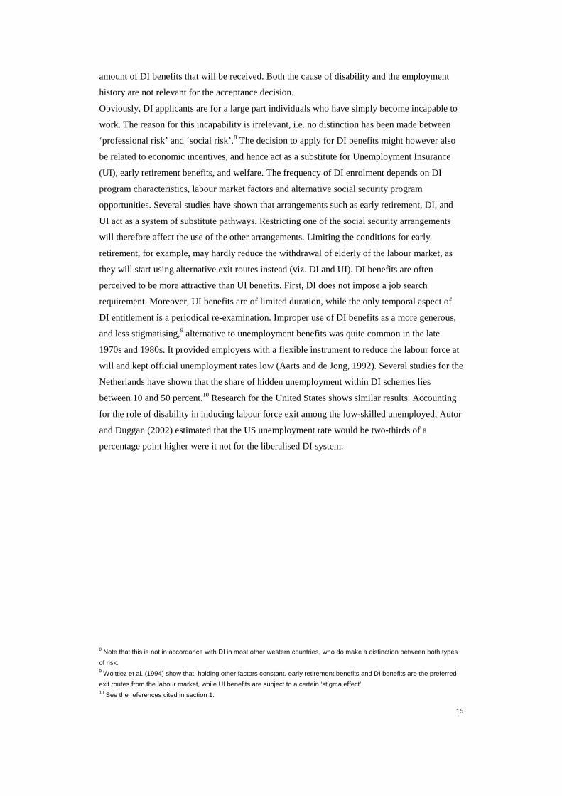
amount of DI benefits that will be received. Both the cause of disability and the employment
history are not relevant for the acceptance decision.
Obviously, DI applicants are for a large part individuals who have simply become incapable to
work. The reason for this incapability is irrelevant, i.e. no distinction has been made between
‘professional risk’ and ‘social risk’.8 The decision to apply for DI benefits might however also
be related to economic incentives, and hence act as a substitute for Unemployment Insurance
(UI), early retirement benefits, and welfare. The frequency of DI enrolment depends on DI
program characteristics, labour market factors and alternative social security program
opportunities. Several studies have shown that arrangements such as early retirement, DI, and
UI act as a system of substitute pathways. Restricting one of the social security arrangements
will therefore affect the use of the other arrangements. Limiting the conditions for early
retirement, for example, may hardly reduce the withdrawal of elderly of the labour market, as
they will start using alternative exit routes instead (viz. DI and UI). DI benefits are often
perceived to be more attractive than UI benefits. First, DI does not impose a job search
requirement. Moreover, UI benefits are of limited duration, while the only temporal aspect of
DI entitlement is a periodical re-examination. Improper use of DI benefits as a more generous,
and less stigmatising,9 alternative to unemployment benefits was quite common in the late
1970s and 1980s. It provided employers with a flexible instrument to reduce the labour force at
will and kept official unemployment rates low (Aarts and de Jong, 1992). Several studies for the
Netherlands have shown that the share of hidden unemployment within DI schemes lies
between 10 and 50 percent.10 Research for the United States shows similar results. Accounting
for the role of disability in inducing labour force exit among the low-skilled unemployed, Autor
and Duggan (2002) estimated that the US unemployment rate would be two-thirds of a
percentage point higher were it not for the liberalised DI system.
8 Note that this is not in accordance with DI in most other western countries, who do make a distinction between both types
of risk. 9 Woittiez et al. (1994) show that, holding other factors constant, early retirement benefits and DI benefits are the preferred
exit routes from the labour market, while UI benefits are subject to a certain ‘stigma effect’. 10 See the references cited in section 1.

16

17
3 Disability Insurance benefits and individual behaviour
Three months before finishing the period on sickness benefits, an individual may apply for DI
benefits. Subsequently, the Dutch Social Benefits Administration (UWV11) decides on the
application. A medical examiner verifies and evaluates (physical) limitations and job
opportunities, and, based on this examination, the DI administrator decides whether or not to
accept the applicant. In case of acceptance, a benefit is awarded for a period of five years, after
which a periodical re-examination takes place. The degree of disability is determined by an
expert, who compares the applicant’s current earnings capacity with his past earnings capacity.
A rejected applicant has the opportunity to appeal. The letter of objection must be sent within
the period mentioned in the rejection letter. Subsequently, the DI administrator reconsiders the
first decision. The application – award – appeal decision is illustrated in figure 3.1. Note that if
an applicant is denied benefits at the reconsideration stage, then he may exercise the option to
have his case considered by court. This is not shown in figure 3.1.
Figure 3.1 Game tree for Disability Application and Award Processa
Individual:(firm)
UWV:
Application Decision
apply do not apply
Award Decision No Benefits
accept reject
Individual: Benefits Appeal Decision
appeal do not appeal
No BenefitsUWV: ReconsiderationDecision
accept reject
Benefits No Benefits
a ‘Benefits’ may either be ‘full benefits’ or ‘partial benefits’ (the latter in case of partial disability).
DI, as well as other employee insurances, suffer from the problem of moral hazard (see, e.g.,
Barr, 1993). Imperfect information of the DI administrator in the award and reconsideration
decisions leads to higher DI enrolment as a result of an adjustment in the behaviour of the
insured population. A second form of moral hazard may be a lack in prevention efforts. In this
respect, the DI application and appeal decisions of an individual can be regarded as choices
11 There used to exist five different administration offices, which merged into UWV in 2000.

18
between consumption and leisure, given institutions, health conditions, personal characteristics,
working conditions and the expected probability of being granted DI benefits.12 Obviously, for
many applicants this labour supply decision will be severely constrained by their health status.
These individuals will show high demand for leisure irrespective of the financial conditions
involved. Nonetheless, the moral hazard problem just described, together with existing
empirical evidence (mainly for countries outside the Netherlands), suggests that factors other
than health play a significant role in the behaviour of individuals, in particular financial
incentives (see section 1). Thus, individuals who are less constrained by their health status are
likely to be sensitive to financial incentives, and raise their demand for leisure as it becomes
cheaper (that is: as the DI replacement rate becomes higher).
12 Note that the problem of moral hazard equally applies to the employer’s behaviour (Aarts en de Jong, 1992; Koning,
2004). This is however beyond the scope of this paper.

19
4 Data
4.1 Replacement rates
As was already mentioned in section 2, the exact DI benefit conditions are the result of
negotiations by employers’ organisations and trade unions. These negotiations, which mostly
take place at the sector or firm level, are laid down in collective labour agreements. In the
period that will be under consideration, the negotiated collective labour agreements at the sector
level were made compulsory by the government for all firms in that sector. The resulting
variation in replacement rates over different sectors and firms is exactly the variation we will
exploit to identify the elasticity of DI enrolment with respect to the financial incentives
involved. The pitfalls involved in this approach will be discussed in later sections.
A database with information on replacement rates for different sectors is available through the
Netherlands’ Labour Inspectorate. We have made a selection of sectors, such that we were able
to match their codes with the sector codes in our data set of individuals. This is necessary in
order to be able to connect both data sets and perform an analysis at the micro level (this will be
further discussed in section 4.2). The resulting selection of sectors, with corresponding
replacement rates, is given in table A.1 (see Appendix A). The reported financial indicators are
the replacement rate for year t (denoted by RRt), and the DI wealth rate (DIWR). This latter
variable is defined as the ratio of the sum of all discounted future DI benefits to current income.
This definition allows us to conveniently rewrite this indicator in terms of replacement rates RRt
in year t:13
(4.1) ( ) ,1
13
2
211
1
1
10
0RRRRRRRRyRR
yDIWR
t
tt
t
tt ρ
ρρρρ−
++=== ∑∑ ∞
=
−∞
=
−
where y0 denotes current income, ρ is a constant discount factor, and RR3 is the replacement rate
in the third year and years ahead (i.e. the replacement rate remains constant from the third year
on).
It can be seen that the average replacement rate in the first year equals 89 percent of the last
earned wage, while the second and third year show average replacement rates of 75 and 70
percent, respectively. Thus, the additional benefits on top of the ‘official replacement rate’ of 70
percent are especially high in the first year of disability. As was noted in section 2.1, the 1993
reform implied that the earnings related benefits became of limited duration, but that this loss in
benefits was ‘repaired’ in most cases. In table A.1 it becomes clear that nearly all sectors
13 Note that next to this definition we will also employ an alternative definition of the DI Wealth Rate later on in the empirical
section, where t will be bounded by the official retirement age of 65.

20
supplement DI benefits from the third year on to 70 percent of the last earned wage. Two
sectors even have a higher replacement rate for these years of respectively 75 percent (joinery
works) and 80 percent (road transport). Most of the variation in replacement rates over different
sectors is however in the first and second year. The range of replacement rates in both years is
from 70 to 100 percent. The variation in DIWR is however equally affected by the variation in
RR1, RR2 and RR3, respectively. This can be seen from the decomposition:
(4.2)( )
,1
21
221
)( 23
3
13
2
12232
422
221
2 σρ
ρσρ
ρρσσρ
ρσρσσ−
+−
++−
++=DIWR
where σi denotes the sample standard deviation of RRi and σij denotes the sample covariance
between RRi and RRj. The term in front of 23σ inflates the contribution of the variation in RR3
to DIWR. It turns out that at the discount factor of 0.9, loosely stated, about one third of the
variation in DIWR is caused by variation in RR1, one third is caused by variation in RR2, and
one third is caused by variation in RR3. At this discount factor level, the ‘DI wealth’ is seen to
equal 7.3 year salaries, with a minimum of 7 year salaries (6 different sectors) and a maximum
of 8 year salaries (road transport). A lower discount factor will however result in a lower weight
of RR3 in DI wealth, and generally in lower DI wealth.
4.2 Micro data
The Dutch Income Panel dataset “IPO” is based on administrative data from the Dutch National
Tax Office and was initiated in 1984.14 Since 1989, the dataset consists of a panel of about
75,000 individuals, who are randomly drawn from the Dutch population provided that they
were 15 years or older and enlisted in the Dutch municipal registers. Attrition occurs only as a
result of emigration or death. In that case new individuals are added to the sample to keep the
total number of individuals at the same level. For each individual drawn into the sample several
variables are available, which can be divided into three groups:
� Variables concerning individual characteristics, such as gender, date of birth, and a variable
indicating the sector in which the individual was working;
� Variables concerning household characteristics, such as the number of persons in the
household, the number of minor children (age categories) and marital status;
� Financial variables, such as the level of the income, and the source of the income (e.g. wage
income, pension benefit, DI benefit, UI benefit). The observation of these variables is in
principle on a yearly basis, and relates both to household and individual income. Also, some
14 The acronym IPO stands for “Income Panel Study” (in Dutch: Inkomens Panel Onderzoek).

21
other financial variables are available, such as outstanding mortgage and real estate appraisal
(the so-called “WOZ-value”).
The IPO dataset not only contains information on the individuals selected into the sample, but
also on the other persons in the households they belong to. These last individuals will also be
included in our sample. A great advantage of this dataset is that the observed variables are
measured with high accuracy. A drawback of the IPO dataset is however that it lacks some
crucial variables which are not related to the household and financial situation of individuals,
most notably education and health status.
For our empirical analysis we use data from the period 1996-2000. We select those individuals
into our sample who are eligible for receiving DI benefits in case of disability. That is, all
individuals with positive wage income on December 31 of the years 1995 until 1999 are
selected into our sample. These are precisely the individuals who might enter DI in the
subsequent years. Thus, according to our definition, an individual enters the DI scheme when he
receives wage income at the beginning of the year (formally, on the last day of the previous
year) and receives a DI benefit at some other moment of the year. Note that, as a result of this
selection process, the self-employed are also removed from our sample. This is correct, as the
self-employed have their own Disability Insurance, which is different from the DI for
employees considered in this paper.
In order to assess the effect of financial incentives on the probability of entering the DI scheme,
the replacement rates of the Dutch Labour Inspectorate are linked to the individuals in the IPO
dataset. For this we use the variable in the dataset that indicates the sector in which an
individual is working. An overview of the replacement rates of sectors used in this chapter was
given in table 4.1. Since no substantial changes in replacement rates have occurred in the period
1996-2002, we have linked these figures to the individuals in the IPO dataset for the period
1996-2000. Note that the incomplete observation of replacement rates at the individual level
implies that we are able to select only about 10% of the individuals into our sample.
The resulting dataset is the core file we use for the empirical analysis. It is an unbalanced
dataset with 97950 observations (including multiple observations per individual) during the
period 1996 - 2000. Within this period 448 of the 97950 observations enter the DI scheme
(0.46%). Note that the actual macro figures concerning DI inflow are higher: over the period
concerned the average macro DI enrolment figure was 1.2% (Lisv, various years). For a part
this can be explained from the fact that our sample is not representative for the entire Dutch
population. For instance, the sample does not include the social service sector and the public
sector. For another part it follows from the fact that we have multiple observations per person.
The observed inflow percentage however still remains low. The frequencies of some important

22
groups in the sample are presented in table 4.2, together with their DI enrolment (%). This table
shows that 26% of the individuals in the dataset consist of women, of which 0.52% enter the DI
scheme during the period 1996-2000. Older individuals have a higher DI enrolment during this
period than younger individuals. The household characteristics indicate that couples have a
higher DI enrolment than singles. Households with children have a lower DI enrolment than
households without children. The construction sector shows a higher DI enrolment figure than
other sectors.
Table 4.1 Sample characteristics IPO, 1996-2000
In sample (% of sample size) Disability enrolment (% of concerning category)
Total 100.0 0.46
Woman 26.1 0.52
Man 73.9 0.44
Age, until 29 28.6 0.16
Age, 30 to 34 13.3 0.42
Age, 35 to 39 14.8 0.43
Age, 40 to 44 14.1 0.56
Age, 45 to 49 12.9 0.60
Age, 50 to 54 10.2 0.73
Age, 55 to 59 5.0 1.12
Age, above 60 1.2 0.62
Couple 73.5 0.54
Single 26.5 0.23
With children 53.3 0.39
No children 46.7 0.54
Manufacturing sector 26.9 0.38
Construction sector 26.3 0.59
Trade and Food sector 33.6 0.39
Transport and Storage sector 13.3 0.50

23
5 Empirical strategy
As was discussed in section 3, DI program participation results from two contingencies: the
probability that a worker claims to be disabled and applies for DI benefits, and the probability
that the claim will be awarded by the program administrator. In most previous research the
typical approach has been to estimate a single reduced form model of the final allowance
decision. The main reason for this is the lack of data needed to identify the parameters which
govern the separate stages of the process. Our analysis will be no exception to this line of
research. In contrast, a number of studies were able to estimate a multistage model describing
the various stages of the application and award decision (e.g. Lahiri et al., 1995; Riphahn and
Kreider, 1998; Benitez-Silva et al., 1999).
In the previous section it appeared that the observed inflow probabilities in the IPO sample are
substantially lower than the aggregate figures (see table 4.2). This could be the result of
incomplete observation of DI enrolment, since the administrations of the National Tax Office
and the DI Administration Office are separate. In this section we discuss a strategy which is
robust to this problem, provided that the underlying process is correctly specified by the Logit
model. Two types of incomplete observation are distinguished. First, it may be the case that
individuals entering DI somehow disappear from the sample before it is indicated that they
actually receive DI benefits. Second, it may be the case that individuals entering DI remain in
the sample but have their status misreported. That is, they are being characterised as working
while they are on (partial) DI benefits. In the econometric literature, the first case is known as
endogenous selection, while the second is known as misclassification. In the following, we label
these as incomplete observation of type I and type II, respectively. In addition, we specify the
log-likelihood for our sample subject to the bounded Logit model, and briefly discuss the
Hosmer-Lemeshow test in the context of this model.
5.1 Incomplete observation
Define Y as the variable indicating whether DI enrolment takes place (Y=1) or not (Y=0), and
suppose that this event can be modelled through the well-known Logit model:
(5.1) ,)'exp(1
)'exp(}1Pr{1 β
βx
xYp
+===
where the vector x contains a range of explanatory variables, including a full set of sector-
specific dummy variables (or alternatively, a constant and a set of sector-specific dummy
variables related to a ‘reference sector’). Under certain regularity conditions, Maximum
Likelihood estimation based on (5.1) will produce consistent and efficient estimates of the

24
parameter vector β (see, e.g., Cramer, 2003). One of these regularity conditions is that
observations in the sample are randomly selected from the population. However, in case some
of the observations with Y=1 have somehow disappeared from the sample this condition is
violated. That is, observations with Y=1 are endogenously selected into the sample.
Proposition 1. Suppose that
(i) Y is correctly specified by the Logit model
(ii) Y may be incompletely observed (type I)
Then maximisation of the likelihood based on the Logit model produces consistent and efficient
estimates for all coefficients β in the Logit model, except for the sector-specific dummies (and
the intercept, if included).
First, consider the general case where sample selection occurs with the same probability in
every sector. Denote with γ the probability that an observation with Y=1 is selected into the
sample (0<γ≤1). It is well-known that in a general discrete choice model, consistent parameter
estimates can be obtained through maximisation of the likelihood based on15
(5.2) ,~
10
11 pp
pq
γγ+
=
where p0=1-p1. In the literature, this procedure is often called ‘pseudo-likelihood estimation’ or
‘pseudo-maximum likelihood estimation’. Now with the Logit model in (5.1) it can be readily
checked that
(5.3) .)ln'exp(1
)ln'exp(~1 γβ
γβ++
+=
x
xq
This familiar property implies that estimation of the binary Logit model on an endogenous
sample will produce consistent and efficient parameter estimates, provided that a constant term
is included in the vector x. The ‘true value’ for β0 can only be retrieved if γ is known
beforehand. The asymptotic standard error of this coefficient also needs a simple adjustment
(see, e.g., Scott and Wild, 1997). Generalisation of this result to the case where the endogenous
selection rule differs by sector is straightforward. Suppose that the probability that an individual
entering DI is included in the sample equals γj for sector j. Equation (5.3) then becomes:
(5.4) .)ln'exp(1
)ln'exp(1
j
j
x
xq
γβγβ
++
+=
15 See Hsieh et al. (1985). The case considered here is the binary discrete choice model with endogenous selection on one
outcome, but the result equally applies to multinomial discrete choice models with multiple selection rules for different
outcomes of Y.

25
The implication is that Maximum Likelihood estimation will again produce consistent and
efficient parameter estimates provided that a full set of sector specific dummy variables is
included. Similar to the case with the ‘general’ selection rule in (5.3), consistent estimators for
these dummy variables can only be retrieved if the factors γj are known, while asymptotic
standard errors for these dummy variables need to be adjusted. We now turn to the more general
case, where both incomplete observation of type I and type II may be present.
Proposition 2. Suppose that
(i) Y is correctly specified by the Logit model
(ii) Y may be incompletely observed (type I and/or type II)
Then maximisation of the likelihood based on the bounded Logit model produces consistent and
efficient estimates of all coefficients β in the Logit model, except the sector-specific dummies
(and the intercept, if included).
Suppose that a fraction of the observations not having “Y=1” is incorrectly observed, that is16
(5.5) }1|0Pr{ === ZYπ
is greater than zero. Here the observed binary variable is denoted by Y, while the true score is
denoted by Z. Now if we assume the Logit model – either with or without endogenous selection
on “Y=1” (equations (5.1) and (5.4), respectively) – then the probability of observing DI
enrolment equals
(5.6) ).1()1}(0|0Pr{}1|0Pr{1}1Pr{ 1111 π−=−==+==−=== qqZYqZYYr
Hence, the probability of observing “Y=1” equals
(5.7) .)ln'exp(1
)ln'exp()1(1
j
j
x
xr
γβγβ
π++
+−=
This model is identical to the so-called ‘bounded Logit model’ (see, e.g., Cramer, 2004). Note
that the specification is derived under the assumption that misspecification chronologically
follows endogenous selection (type II follows type I). If this schedule is reversed, then the
resulting model is simply Logit.17
16 See Hausman et al. (1998) for a more general treatment of the topic. 17 The concerning model is (5.4) with the argument x’β+ln(γj) replaced by x’β+ln(γj)+ln(1-π).

26
5.2 Estimation and testing
Our likelihood is based on (5.7), and writes as:
(5.9) { },)),,(1ln()1(),,(ln),(1
11∑=
−−+=n
iiiii xryxry πβπβπβl
where observations are indexed by i, the total number of observations in the sample is n, and yi
indicates DI enrolment for observation i. In (5.9) the coefficients γj are suppressed, as these
cannot be identified separately from the firm-specific dummy variables contained in β. Each
observation corresponds to an individual in a specific year, so that we may have multiple
observations for a given individual. The inclusion of individual specific effects into our model
is however not an attractive option, as it involves both theoretical and practical problems. First,
it is well-known that Maximum Likelihood (ML) estimation with the individual fixed effects as
parameters alongside β causes the estimates of the latter to be inconsistent.18 A second, more
practical problem, is that this involves the addition of a vast number of parameters (in our case
over 30,000!). The alternative approach, which overcomes these two problems, uses ΣiœA(i,j) yi as
a sufficient statistic for the fixed effect of individual j and consistently estimates β from the
likelihood conditional on this sufficient statistic (A(i,j) denotes the set of observations {i} which
correspond to individual j). This approach is however also problematic because it implies that
the model is only identified from the ‘within’ dimension of the data, which in our case means
that only the individuals entering DI contribute to the likelihood, while others (99,5% of our
data) are discarded. A second problem with this alternative approach is that no ‘average partial
effects’ or elasticities can be computed, as the fixed effects distribution remains unknown. The
second alternative to pooled estimation, the inclusion of random effects, is also not very
attractive as it involves the rarely satisfied assumption that these random effects are
uncorrelated with the covariates in x. In fact, in a recent Monte Carlo study Greene (2003) finds
that random effects estimation is inferior to both fixed effects and pooled estimation.19 His
results further suggest that the pooled estimator performs better if the number of observations
per individual (i.e. the number of elements in A(i,j)) is small, while the fixed effects estimator
(full estimation) does relatively better if the number of observations per individual increases.
For our case, this is another argument in favour of the pooled model, as the number of
observations per individual is at most 4.
Theoretically, the ML estimate of β not only is inconsistent in the random effects and fixed
effects (full estimation) model, but also in the pooled model. In particular, the latter will lead to
attenuated estimates of β (see Wooldridge, 2002, pp. 470-472). However, Greene’s Monte
18 See Lancaster (2000) for a survey on this ‘incidental parameters problem’. 19 For this matter, the author has presented results for the Probit model, but these are likely to carry over to the Logit model.

27
Carlo results suggest that this attenuation bias might be small – in particular for continuous
covariates. Moreover, our concern is primarily with the elasticity of r1 with respect to variables
xj (in particular DIWR), which is less sensitive for the neglect of unobserved heterogeneity than
the parameters in β; see Appendix B.
In the discussion of the previous subsection it has become clear that the assumption of the Logit
specification is crucial for our analysis. It is therefore necessary to test this assumption. For
instance, we can test whether the predicted fraction with Y=1 in the sample is consistent with
the shape of the (bounded) Logit curve. Suppose that the observations are ordered into G
different groups by their predicted probabilities r1(i) for individual i, i.e.:
(5.10) ),(min)(max 1)(
1)1(
irirgIigIi ∈−∈
≤
for all g=2, ..., G, and I(g) is the set of individuals in group g. Denote with ng the number of
observations in group g, with fg the fraction of observations in this group with Y=1, and with
r1(g) the average predicted probability of Y=1 for this group. Under the null hypothesis that the
observations are in accordance with the (bounded) Logit model, the Hosmer-Lemeshow test
statistic
(5.11) ∑= −
−=
G
g
gg grgr
grfnC
1 11
21
))(1)((
))((
has a chi-square distribution with G-2 degrees of freedom (Hosmer and Lemeshow, 1980;
2000). When small probabilities are involved, Cramer (2003, 2004) advocates the use of groups
with equal numbers of observations. The point is that if the composition of the groups is based
on percentiles of r1, then the sample population will be extremely unevenly distributed across
different groups, so that the test loses much of its power.

28

29
6 Estimation results
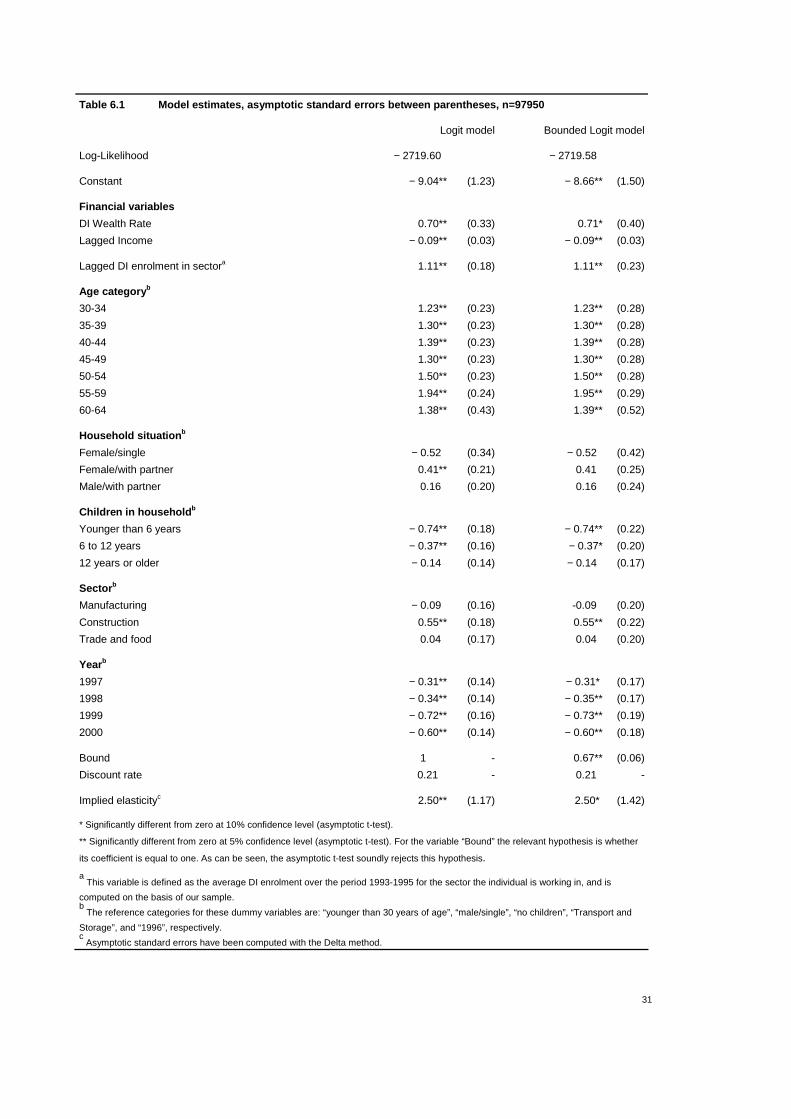
The estimation results for both the Logit and the bounded Logit model are shown in table 6.1.
While the bound in the latter model is significantly different from one at a 5% confidence level,
it can be seen that the point estimates of all other parameters are hardly different from those in
the Logit model. The most important difference concerns the (asymptotic) confidence intervals
which become somewhat wider in the bounded Logit model. As a consequence, the asymptotic
t-test for the hypothesis that a parameter equals zero shows diverging results for a few variables.
The score in the bounded Logit model is somewhat better than in the Logit model, though not
convincingly so.
The specification includes both the lagged DI enrolment per sector as well as dummy variables
for each (broadly defined) sector, in an attempt to correct for sector-specific effects. Lagged DI
enrolment is determined over the same sectors as the DI Wealth Rate (see Appendix A), but can
be identified separately from the latter as it varies more over different sectors.20 This variable is
likely to be a good first predictor for the individual enrolment probability, and indeed the
concerning estimate is close to unity. Furthermore, the significantly positive dummy variable
for the Construction sector suggests that, after controlling for individual, household and
financial variables, the individual risk of DI enrolment is higher in that sector than in the others.
This seems plausible, as the work in this sector is in general physically more demanding.
However, if incomplete observation of type I (endogenous selection) plays a role here, then
both the magnitude and the asymptotic t-statistic for the “Construction” sector are biased
downward, so that the estimate may even be on the conservative side.21
As was apparent in (4.1), the DI Wealth Rate nonlinearly depends on the discount factor ρ. It
turned out to be difficult numerically to find the optimal value for this parameter, so that we
have repeatedly estimated both models for fixed values of ρ and finally reported those estimates
for which the log-Likelihood attained its maximum value. For both the Logit and the bounded
Logit model the optimal value for ρ was 0.79, implying an individual discount rate of 21%.22
The estimation results are however rather insensitive for (local) variations in ρ. The point
estimate for the DI Wealth Rate parameter equals 0.70 and 0.71 for the Logit and the bounded
Logit model, respectively, which translates into an elasticity of DI enrolment with respect to the
DI Wealth Rate of 2.5 (in both models). The coefficient of 0.71 in the bounded Logit model
implies a marginal effect of 3.25·10-3. Thus, our model predicts that a constant replacement rate
20 In fact, the correlation between both variables (over the sample of individuals) amounts no more than 0.11. 21 See subsection 5.1, and Scott and Wild (1997) for technical details. 22 This grid search was performed over the set {0.700; 0.705; 0.710; ...; 1.000}.

30
of 75% implies a 17% higher probability on DI enrolment than a constant replacement rate of
70%.23
The other parameter values mostly show their expected signs. The risk of DI enrolment tends to
become higher for higher ages. The exception is the age category of 60 to 64, which shows a
lower risk than the two younger categories. This can be attributed to the relatively high
relevance of the ‘competing risks’ of unemployment and (official) early retirement. A second
explanation is that we have only few observations in this age category (i.e. few individuals
having paid work; see table 4.2), so that small sample bias may play a role. For women, it is
seen that living together with a partner increases the risk of DI enrolment, while for men there
does not appear to be an effect. On the other hand, having young children appears to have a
negative impact on the propensity to DI enrolment. There is no obvious explanation for this.
Perhaps parents have a larger incentive to earn sufficient income in order to satisfy the needs of
their children.
23 A constant replacement rate of 70% and 75% respectively implies a DIWR of 333.33 and 357.14 (both computed at the
discount rate of 21%). Hence, the estimated effect on the enrolment probability equals (3.25·10-3)·(357.14-333.33)=17%.
31
Table 6.1 Model estimates, asymptotic standard errors between parentheses, n=97950
Logit model Bounded Logit model
Log-Likelihood − 2719.60 − 2719.58
Constant − 9.04** (1.23) − 8.66** (1.50)
Financial variables
DI Wealth Rate 0.70** (0.33) 0.71* (0.40)
Lagged Income − 0.09** (0.03) − 0.09** (0.03)
Lagged DI enrolment in sectora 1.11** (0.18) 1.11** (0.23)
Age categoryb
30-34 1.23** (0.23) 1.23** (0.28)
35-39 1.30** (0.23) 1.30** (0.28)
40-44 1.39** (0.23) 1.39** (0.28)
45-49 1.30** (0.23) 1.30** (0.28)
50-54 1.50** (0.23) 1.50** (0.28)
55-59 1.94** (0.24) 1.95** (0.29)
60-64 1.38** (0.43) 1.39** (0.52)
Household situationb
Female/single − 0.52 (0.34) − 0.52 (0.42)
Female/with partner 0.41** (0.21) 0.41 (0.25)
Male/with partner 0.16 (0.20) 0.16 (0.24)
Children in householdb
Younger than 6 years − 0.74** (0.18) − 0.74** (0.22)
6 to 12 years − 0.37** (0.16) − 0.37* (0.20)
12 years or older − 0.14 (0.14) − 0.14 (0.17)
Sectorb
Manufacturing − 0.09 (0.16) -0.09 (0.20)
Construction 0.55** (0.18) 0.55** (0.22)
Trade and food 0.04 (0.17) 0.04 (0.20)
Yearb
1997 − 0.31** (0.14) − 0.31* (0.17)
1998 − 0.34** (0.14) − 0.35** (0.17)
1999 − 0.72** (0.16) − 0.73** (0.19)
2000 − 0.60** (0.14) − 0.60** (0.18)
Bound 1 - 0.67** (0.06)
Discount rate 0.21 - 0.21 -
Implied elasticityc 2.50** (1.17) 2.50* (1.42)
* Significantly different from zero at 10% confidence level (asymptotic t-test).
** Significantly different from zero at 5% confidence level (asymptotic t-test). For the variable “Bound” the relevant hypothesis is whether
its coefficient is equal to one. As can be seen, the asymptotic t-test soundly rejects this hypothesis.
a This variable is defined as the average DI enrolment over the period 1993-1995 for the sector the individual is working in, and is
computed on the basis of our sample. b The reference categories for these dummy variables are: “younger than 30 years of age”, “male/single”, “no children”, “Transport and
Storage”, and “1996”, respectively. c Asymptotic standard errors have been computed with the Delta method.

32
Results of the Hosmer-Lemeshow test are shown in table 6.2 and figure 6.1, with group sizes
equalling 9794 or 9795. The resulting test statistic equals 13.1, which is lower than the 5%
critical value of 15.5. Thus, the bounded Logit model cannot be rejected. The last two columns
in table 6.2, and figure 6.1, indeed show that the ‘curvature’ of the predicted probabilities
indeed does not deviate too much from the postulated curvature of the bounded Logit model.
Note that on the basis of this statistical test the plain Logit model can also not be rejected, with
a test statistic equalling 11.8 at the same critical value as above.
Table 6.2 Hosmer-Lemeshow test (with equal group sizes) of the bounded Logit model
Number of observations in
interval
Lower bound (%) Upper bound (%) Average predicted
probability of DI
enrolment (%)
Observed fraction of
DI enrolment (%)
9794 0.00 0.10 0.10 0.07
9795 0.10 0.15 0.08 0.12
9795 0.15 0.21 0.13 0.18
9795 0.21 0.27 0.28 0.24
9795 0.27 0.34 0.38 0.30
9795 0.34 0.43 0.34 0.39
9795 0.43 0.55 0.38 0.49
9795 0.55 0.70 0.60 0.62
9795 0.70 0.95 0.97 0.81
9795 0.95 6.13 1.32 1.36
Figure 6.1 Fit of the predicted probabilities for ten equally sized groups in the bounded Logit model
0.00%
0.20%
0.40%
0.60%
0.80%
1.00%
1.20%
1.40%
1.60%
[0;0
.10]
[0.1
0;0.
15]
[0.1
5;0.
21]
[0.2
1;0.
27]
[0.2
7;0.
34]
[0.3
4;0.
43]
[0.4
3;0.
55]
[0.5
5;0.
70]
[0.7
0;0.
95]
[0.9
5;6.
13]
observed predicted

33
In Table 6.3, estimation results for alternative specifications are reported. Variants 1 and 2 are
the ‘extreme cases’ of incomplete observation, the first with exclusively type I (endogenous
selection) present and the second with exclusively type II (misspecification). The elasticity
estimate appears quite robust, as both ‘extremes’ remain quite close to the basic estimate.
Variants 3-6, a lower discount rate and alternative sector-specific enrolment variables, imply
somewhat higher elasticity estimates, but lower likelihoods.
Table 6.3 Sensitivity analysis
Specification Likelihood Bound Implied elasticity with respect to DIWRa
0. Basicb − 2719.58 0.67 2.50 (1.42)
1. Bound equal to 1b − 2719.60 1 2.50 (1.17)
2. Bound equal to 0.46/1.2c − 2719.66 0.38c 2.59 (1.89)
3. Discount rate = 10% (ρ=0.9) − 2720.02 0.50 3.17 (2.54)
4. DIWR with cut-off at age 65d − 2720.14 0.68 3.21 (1.77)
5. Lagged variable = Enrolment in past year − 2725.58 0.68 3.82 (1.41)
6. Lagged variable = Average enrolment in
past three years
− 2728.75 0.82 3.75 (1.27)
a Asymptotic standard errors are reported between parentheses.
b These specifications correspond to those reported in table 6.1.
c In this variant, the bound in the bounded Logit model is fixed at a value equal to the sample average probability of DI enrolment divided
by the actual (macro) probability of DI enrolment. The latter has been computed as an average over all relevant years (also see section
4.2). d In this variant, the DI Wealth Rate was summed over the time periods 1 until T, where T equals the number of years until the official
retirement age 65. That is, the new formula for DIWR simply follows from replacing ∞ by T in (4.1). The reported results correspond with
a discount rate of 14%, which turned out to be optimal with this definition of DIWR.

34

35
7 Conclusion and directions for further research
In this paper, we have estimated the impact of the financial conditions in Disability Insurance
(DI) on the individual’s probability of DI enrolment. We have found that individuals with
relatively high DI Wealth (that is, the ratio of foreseen DI benefits to current income) are more
likely to enrol. Based on variation in DI replacement rates between different sectors, the
concerning elasticity was estimated at a value of 2.5. In estimating this elasticity, we have
controlled for individual and household specific characteristics, and have tried to correct for
sector specific effects (other than financial conditions) and the possibility of incomplete
observation of DI enrolment.
A possible problem we have not been able to address is that DI replacement rates may in the
long term depend on the risk of DI enrolment. That is, labour unions have a stronger incentive
to negotiate high replacement rates if the risk of DI enrolment is higher. If this is really the case,
then our estimated elasticity may overestimate the true effect. Taking account of such a
mechanism will however prove difficult, as no appropriate instruments24 appear to be available.
A second point which is left for future research is that the current elasticity has been estimated
at given eligibility criteria. It is however likely that the elasticity depends (negatively) on
eligibility strictness, so that the evaluation of policy measures including a modification in
eligibility criteria would require more precise knowledge of this interdependence.
24 That is, variables influencing the replacement rate, but not DI enrolment. A possibility is to estimate a simultaneous model
for DI enrolment and the DI replacement rates, but this would require data over a longer time period. The problem with such
a long time period is data inconsistency; e.g. the definitions of sectors have changed (in 1993), and the composition of
sectors has also changed over the years.

36

37
References
Aarts, L., and P. de Jong, 1992, Economics Aspects of Disability Behaviour, Amsterdam, North
Holland.
Autor, D., and M. Duggan, 2002, The Rise in Disability Recipiency and the Decline in
Unemployment, MIT Dept. of Economics Working Paper No. 01-15, Cambridge, MIT.
Barr, N., (1993), The Economics of the Welfare State, London, Weidenfeld and Nicholson.
Benitez-Silva, H., M. Buchinsky, H. Chan, J. Rust, and S. Sheidvasser, 1999, An Empirical
Analysis of the Social Security Disability Application, Appeal, and Award Process, Labour
Economics, 6, 147-178.
Black, D., K. Daniel, and S. Sanders, 2002, The Impact of Economic Conditions on
Participation in Disability Programs: Evidence from the Coal Boom and Bust, American
Economic Review, 92, 27-50.
Bosch, van den, F., and C. Petersen, 1983, An Explanation of the Growth of Social Security
Disability Transfers, De Economist, 131, 65-79.
Bound, L., and R. Burkhauser, 1999, Economic Analysis of Transfer Programs Targeted on
People with Disabilities. In: O. Ashenfelter and D. Card, eds., Handbook of Labor Economics,
volume 3C, Amsterdam, North Holland.
Cramer, J., 2003, Logit Models from Economics and Other Fields, Cambridge University Press.
Cramer, J., 2004, Scoring Bank Loans that May Go Wrong: a Case Study, Statistica
Neerlandica, 58, 365-380.
Greene, W., 2003, The Behavior of the Maximum Likelihood Estimator of Limited Dependent
Variable Models in the Presence of Fixed Effects, Working paper, Department of Economics,
New York University.
Gruber, J., 2000, Disability Insurance Benefits and Labour Supply, Journal of Political
Economy, 108, 1162-1183.
Hassink, W., 1996, Worker flows and the employment adjustment of firms, PhD thesis, Vrije
Universiteit Amsterdam, Amsterdam/Rotterdam, Tinbergen Institute.

38
Hassink, W., 2000, Job Destruction through Quits or Layoffs?, Applied Economics Letters, 7,
45-47.
Hassink, W., J. van Ours, and G. Ridder, 1997, Dismissal through Disability, De Economist,
145, 29-46.
Hausman, J., J. Abrevaya, and F. Scott-Morton, 1998, Misclassification of the Dependent
Variable in a Discrete-response Setting, Journal of Econometrics, 87, 239-269.
Hosmer, D., and S. Lemeshow, 1980, Goodness of Fit Tests for the Multiple Logistic
Regression Model, Communications in Statistics, A10, 1043-1069.
Hosmer, D., and S. Lemeshow, 2000, Applied Logistic Regression, 2nd edition. New York,
Wiley.
Hsieh, D., C. Manski, and D. McFadden, 1985, Estimation of Response Probabilities from
Augmented Retrospective Observations, Journal of the American Statistical Association, 80,
651-662.
Kapteyn, A., and K. de Vos, 1999, Social Security and Retirement in the Netherlands, in: J.
Gruber and D. Wise (eds.), Social Security and Retirement around the World, Chicago,
University Press, 269-304.
Kerkhofs, M., M. Lindeboom, and J. Theeuwes, 1999, Retirement, Financial Incentives and
Health, Labour Economics, 6, 203-227.
Koning, P., 2004, Estimating the impact of experience rating on the inflow into Disability
Insurance in the Netherlands, CPB Discussion Paper 37, The Hague, CPB Netherlands Bureau
for Economic Policy Analysis.
Lancaster, A., 2000, The Incidental Parameters Problem since 1948, Journal of Econometrics,
95, 391-414.
Lahiri, K., D. Vaughan, and B. Wixon, 1995, Modeling SSA’s Sequential Disability
Determination Process using Matched SIPP Data, Social Security Bulletin, 58, 3-42.
Lindeboom, M., 1998, Microeconometric analysis of the retirement decision: the Netherlands,
OECD Working Paper 20, Paris, OECD.

39
Lisv, various years, Ontwikkeling arbeidsongeschiktheid, jaaroverzichten 1996, 1997, 1998,
1999 en 2000, Amsterdam, Landelijk instituut sociale verzekeringen.
OECD, 2003, Transforming Disability into Ability; Policies to Promote Work and Income
Security for Disabled People, Paris, OECD.
Riphahn, R., and B. Kreider, 1998, Applications to the U.S. Disability System: A
Semiparametric Approach for Men and Women, IZA Discussion Paper, 17, Bonn, IZA.
Roodenburg, H., and W. Wong Meeuw Hing, 1985, De arbeidsmarktcomponent in de WAO,
CPB Occasional Paper, 34, The Hague, CPB Netherlands Bureau for Economic Policy
Analysis.
Scott, A., and C. Wild, 1997, Fitting Regression Models to Case-Control Data by Maximum
Likelihood, Biometrika, 84, 57-71.
Social and Economic Council of the Netherlands, 2002, Werken aan arbeidsgeschiktheid, SER
rapport 5, The Hague, SER.
Westerhout, E., 1996, Hidden unemployment in Dutch disability schemes, CPB Report, 1996/2,
24-29.
Woittiez, I., M. Lindeboom, and J. Theeuwes, 1994, Labour Force Exit Routes of the Dutch
Elderly: A Discrete Choice Model, in: A. Bovenberg (ed.), The Economics of Pensions: The
Case of the Netherlands, pp. 1-23, Rotterdam, Ocfeb.
Wooldridge, J., 2002, Econometric Analysis of Cross Section and Panel Data, Cambridge, MIT
Press.

40

41
Appendix A. Replacement rates per sector
Table A.1 Overview of replacement rates of sector collective labour agreements, 2002
Sector Code a Category b Name RR1 c RR2 RR3 DIWR d
158 1 Manufacture of bread, fresh pastry goods and
cakes
85
85
70
728.5
170 1 Manufacture of textiles 100 70 70 730
182 1 Manufacture of wearing apparel and
accessories (excl. leather)
100
70
70
730
203 1 Manufacture of builders' carpentry and joinery 80 75 75 755
212 1 Manufacture of articles of paper and paperboard 100 100 70 757
222 1 Printing and service activities related to printing 100 100 70 757
266 1 Manufacture of articles of concrete, plaster or
cement
100
70
70
730
270 1 Manufacture of basic metals (excl. iron, steel,
and ferro-alloys)
94
70
70
724
271 1 Manufacture of basic iron and steel and of ferro-
alloys
70
70
70
700
280 1 Manufacture of fabricated metal products,
except machinery and equipment
100
70
70
730
342 1 Manufacture of bodies (coachwork) for motor
vehicles; manufacture of trailers and semi-
trailers
100
70
70
730
361 1 Manufacture of furniture 80 70 70 710
400 1 Electricity, gas, steam and hot water supply 90 70 70 720
452 2 Building of complete constructions or parts
thereof; civil engineering
70
70
70
700
453 2 Building installation 100 70 70 730
454 2 Building completion 70 70 70 700
501 3 Sale of motor vehicles 100 70 70 730
513 3 Wholesale of food, beverages and tobacco
(excl. meat and meat products)
90
80
70
729
513 3 Wholesale of meat and meat products 100 70 70 730
514 3 Wholesale of textiles 100 70 70 730
514 3 Wholesale of electrical household appliances
and radio and television goods
100 70 70 730
521 3 Retail sale in non-specialised stores (excl.
stores with food, beverages or tobacco
predominating)
90
80
70
729
522 3 Retail sale of meat and meat products 90 70 70 720
523 3 Dispensing chemists 81.25 70 70 711.25
523 3 Retail sale of medical and orthopaedic goods 90 80 70 729
524 3 Retail sale of hardware, paints, glass, books,
newspapers and stationery
70
70
70
700
524 3 Retail sale of household appliances and radio
and television goods
70
70
70
700
524 3 Retail sale of clothing 70 70 70 700
524 3 Retail sale of footwear and leather goods 70 70 70 700
524 3 Retail sale of textiles 90 70 70 720

42
Table A.2 Overview of replacement rates of sector collective labour agreements, 2002, continued
524 3 Retail sale of furniture, lighting equipment and
household articles
80
75
70
714.5
550 3 Hotels and restaurants 100 90 70 748
552 3 Camping sites and other provision of short-stay
accommodation
100
90
70
748
555 3 Canteens and catering 100 90 70 748
601 4 Transport via railways 90 80 70 729
602 4 Freight transport by road 80 80 80 800
602 4 Scheduled passenger land transport (excl.
railways)
95
85
70
738.5
602 4 Taxi operation 80 70 70 710
640 4 Post and courier activities 85 70 70 715
Sample mean 89 75 70 727
Standard deviation 11 8.7 1.8 20
a Sector codes are according to the so-called ‘SBI 1993’ definition. Note, that we have only reported the 3-digit codes here, while some
sectors are actually defined on the basis of 4-digit codes. b
Sectors are divided into the following categories: 1 = Manufacturing, 2 = Construction, 3 = Trade and food, 4 = Transport and storage. c Replacement rates for year t are denoted by RRt. The replacement rate for the third year remains constant for later years, i.e.:
RR3=RR4=RR5=… d
The DI wealth rate (as a percentage of current income) reported in this column is calculated at a discount rate of 10 percent, i.e. ρ=0.9.
Source: Labour Inspectorate

43
Appendix B. Parameters and implied elasticities: consistent estimation
In a general discrete choice model with probability of success r1, the elasticity of r1 with respect
to xj is given by
(B.1) j
jj x
rx
∂∂
= 1lnε
for some given individual. A consistent point estimate of the elasticity with respect to xj is then
equal to the average of the individual elasticities.25
The question is now: suppose that the process should instead be represented by a specification
r1c with some heterogeneity correction term c, would (B.1) then be correct still? In this case, the
elasticity with respect to xj would equal
(B.2) ,ln 1
∂∂
=j
ccjj x
rExε
where c is a vector which is randomly distributed across the population, and Ec denotes the
expected value operator with respect to c. Thus, (B.1) is consistent if (and only if)
(B.3) .lnln 11
∂∂
=∂
∂
j
cc
j x
rE
x
r
This is a mild condition compared to those needed for consistent estimation of the parameter βj.
For example, all specifications with multiplicative unobserved heterogeneity of the form
(B.4)
+= ∑
=
m
jjjc xccrr
1011 exp
satisfy (B.3). The conclusion is that individual behaviour not necessarily needs to obey a
relatively rigid model specification in order to generate consistent estimates for elasticities, as
long as the ‘average behaviour’ is in accordance with the ‘rigid specification’. A well-known
example is the computation of ‘average partial effects’ (APE’s) in the random effects Probit
25 The standard error of this elasticity can be computed with the well-known Delta method.

44
model (see Wooldridge, 2002, pp. 470-472). If the random effects are ignored, that is if the
Probit model is estimated on the pooled data, then the ML estimates for β are biased towards
zero, but the implied APE’s are still consistent. However, such a general result cannot be
derived for the bounded Logit model, but just illustrates the point we want to make here.