Embed Size (px)
Citation preview
8/3/2019 Andrew Stewart- Constraining cosmological parameters with the cosmic microwave background
http://slidepdf.com/reader/full/andrew-stewart-constraining-cosmological-parameters-with-the-cosmic-microwave 1/93
Constraining cosmological parameters with
the cosmic microwave background
Andrew Stewart
Master of Science
Department of Physics
McGill University
Montreal, Quebec
November 3, 2008
A thesis submitted to McGill University in partialfulfilment of the requirements of the degree
of Master of Science
Andrew Stewart 2008

8/3/2019 Andrew Stewart- Constraining cosmological parameters with the cosmic microwave background
http://slidepdf.com/reader/full/andrew-stewart-constraining-cosmological-parameters-with-the-cosmic-microwave 2/93
In fine, he gave himself up so wholly to the reading of romances, that
a-nights he would pore on until it was day, and a-days he would read
on until it was night; and thus, by sleeping little and reading much, the
moisture of his brain was exhausted to that degree, that at last he lost the
use of his reason. A world of disorderly notions, picked out of his books,
crowded into his imagination; and now his head was full of nothing but
enchantments, quarrels, battles, challenges, wounds, complaints, amours,
torments, and abundance of stuff and impossibilities; insomuch, that all
the fables and fantastical tales which he read seemed to him now as true
as the most authentic histories.
Miguel de Cervantes Saavedra, Don Quixote
ii
8/3/2019 Andrew Stewart- Constraining cosmological parameters with the cosmic microwave background
http://slidepdf.com/reader/full/andrew-stewart-constraining-cosmological-parameters-with-the-cosmic-microwave 3/93
ACKNOWLEDGEMENTS
I would like to thank Robert Brandenberger for supervising all of the work pre-
sented in this thesis, for numerous enlightening conversations, and, in particular,
for his patience. Thanks to Joshua Berger and, especially, Stephen Amsel for mak-
ing their code available and answering many questions regarding the edge detection
method. A big thanks to Eric Thewalt for debugging some parts of the code and mak-
ing many helpful suggestions. I would like to thank the WMAP Science Team for the
use of the image shown in Figure 1–1 and I acknowledge the use of the Legacy Archivefor Microwave Background Data Analysis (LAMBDA). Support for LAMBDA is pro-
vided by the NASA Office of Space Science. Thanks, also, to my family for all of their
support during my time at McGill. Last, but most certainly not least, I would like
to thank Rachel Faust, Guillaume Giroux, Martin Auger, Francois Aubin, Razvan
Gornea, John Idarraga, Amelie Bouchat, Marie-Cecile Piro, Francis-Yan Cyr-Racine,
Aaron Vincent, Nima Lashkari, Jean Lachapelle, Anke Knauf, Jamie Sully and Paul
Franche for useful distractions.
iii
8/3/2019 Andrew Stewart- Constraining cosmological parameters with the cosmic microwave background
http://slidepdf.com/reader/full/andrew-stewart-constraining-cosmological-parameters-with-the-cosmic-microwave 4/93
ABSTRACT
We investigate the constraints which can by applied on two different cosmological
parameters using observations of the cosmic microwave background (CMB). First,
we develop a method of constraining the cosmic string tension, Gµ, which uses the
Canny edge detection algorithm as a means of searching CMB temperature maps
for the signature of the Kaiser-Stebbins effect. We test the potential of this method
using high resolution, simulated CMB temperature maps. By imitating the future
output from the South Pole Telescope project, we find that a bound Gµ < 5.5×10⁻⁸
could potentially be imposed. Second, motivated by the string gas cosmological
model, we examine the constraint levied by the CMB on a blue tilted gravitational
wave spectrum. We find that the CMB cannot provide a tighter bound than those
coming from other observations, the most stringent of which is nT 0.15 from
nucleosynthesis.
iv

8/3/2019 Andrew Stewart- Constraining cosmological parameters with the cosmic microwave background
http://slidepdf.com/reader/full/andrew-stewart-constraining-cosmological-parameters-with-the-cosmic-microwave 5/93
ABREGE
Nous etudions les contraintes qui peuvent etre appliquees sur deux parametres
cosmologiques en utilisant les observations du rayonnement de fond cosmologique
(CMB). Premierement, nous developpons une technique de contrainte de la tension
des cordes cosmiques, Gµ, en utilisant l’algorithme de detection des contours Canny
afin de detecter la signature de l’effet Kaiser-Stebbins dans les cartes de temperature
du CMB. Nous testons le potentiel de cette methode avec des cartes de la temperature
du CMB simulees a haute resolution . En imitant les futures donnees du projet
South Pole Telescope, nous trouvons qu’une limite de Gµ < 5.5 × 10⁻⁸ pourrait
etre imposee. Deuxiemement, dans le cadre du modele cosmologique d’un gaz de
cordes, nous examinons la limite imposee par le CMB sur un spectre des ondes
gravitationnelles incline vers le bleu. Nous trouvons que le CMB ne peut fournir
de contrainte plus stricte que celles provenant d’autres observations, nommement la
nucleosynthese, qui impose deja une limite de nT 0.15.
v
8/3/2019 Andrew Stewart- Constraining cosmological parameters with the cosmic microwave background
http://slidepdf.com/reader/full/andrew-stewart-constraining-cosmological-parameters-with-the-cosmic-microwave 6/93
TABLE OF CONTENTS
ACKNOWLEDGEMENTS . . . . . . . . . . . . . . . . . . . . . . . . . . . . iii
ABSTRACT . . . . . . . . . . . . . . . . . . . . . . . . . . . . . . . . . . . . iv
ABREGE . . . . . . . . . . . . . . . . . . . . . . . . . . . . . . . . . . . . . . v
LIST OF TABLES . . . . . . . . . . . . . . . . . . . . . . . . . . . . . . . . . viii
LIST OF FIGURES . . . . . . . . . . . . . . . . . . . . . . . . . . . . . . . . ix
1 Introduction . . . . . . . . . . . . . . . . . . . . . . . . . . . . . . . . . . 1
2 Constraint on the Cosmic String Tension . . . . . . . . . . . . . . . . . . 6
2.1 Overview . . . . . . . . . . . . . . . . . . . . . . . . . . . . . . . . 62.2 Map Making . . . . . . . . . . . . . . . . . . . . . . . . . . . . . . 13
2.2.1 The Gaussian Component . . . . . . . . . . . . . . . . . . . 18
2.2.2 The String Component . . . . . . . . . . . . . . . . . . . . 212.3 The Canny Edge Detection Algorithm . . . . . . . . . . . . . . . . 27
2.3.1 Non-maximum Suppression . . . . . . . . . . . . . . . . . . 282.3.2 Thresholding with Hysteresis . . . . . . . . . . . . . . . . . 32
2.4 Edge Length Counting . . . . . . . . . . . . . . . . . . . . . . . . 392.5 Statistical Analysis . . . . . . . . . . . . . . . . . . . . . . . . . . 432.6 Results . . . . . . . . . . . . . . . . . . . . . . . . . . . . . . . . . 462.7 Discussion . . . . . . . . . . . . . . . . . . . . . . . . . . . . . . . 55
3 Constraint on the Blue Tilt of Tensor Modes . . . . . . . . . . . . . . . . 60
3.1 Overview . . . . . . . . . . . . . . . . . . . . . . . . . . . . . . . . 603.2 Current Bounds from Other Observations . . . . . . . . . . . . . . 63
3.2.1 Pulsar Timing . . . . . . . . . . . . . . . . . . . . . . . . . 64
vi

8/3/2019 Andrew Stewart- Constraining cosmological parameters with the cosmic microwave background
http://slidepdf.com/reader/full/andrew-stewart-constraining-cosmological-parameters-with-the-cosmic-microwave 7/93
3.2.2 Interferometers . . . . . . . . . . . . . . . . . . . . . . . . . 663.2.3 Nucleosynthesis . . . . . . . . . . . . . . . . . . . . . . . . 69
3.3 Results . . . . . . . . . . . . . . . . . . . . . . . . . . . . . . . . . 71
3.4 Discussion . . . . . . . . . . . . . . . . . . . . . . . . . . . . . . . 734 Conclusions . . . . . . . . . . . . . . . . . . . . . . . . . . . . . . . . . . 77
References . . . . . . . . . . . . . . . . . . . . . . . . . . . . . . . . . . . . . . 79
vii

8/3/2019 Andrew Stewart- Constraining cosmological parameters with the cosmic microwave background
http://slidepdf.com/reader/full/andrew-stewart-constraining-cosmological-parameters-with-the-cosmic-microwave 8/93
LIST OF TABLES
Table page
2–1 Definition of the approximate gradient directions used in the edge de-tection algorithm . . . . . . . . . . . . . . . . . . . . . . . . . . . . 31
2–2 Summary of the ability of the Canny algorithm to make a significant
detection of a cosmic string signal for SPT specific simulations . . . 51
2–3 Summary of the ability of the Canny algorithm to make a significantdetection of a cosmic string signal for simulations corresponding toa hypothetical CMB survey . . . . . . . . . . . . . . . . . . . . . . . 54
viii

8/3/2019 Andrew Stewart- Constraining cosmological parameters with the cosmic microwave background
http://slidepdf.com/reader/full/andrew-stewart-constraining-cosmological-parameters-with-the-cosmic-microwave 9/93
LIST OF FIGURES
Figure page
1–1 The WMAP 5-year TT power spectrum along with recent observa-tional results . . . . . . . . . . . . . . . . . . . . . . . . . . . . . . 4
2–1 The geometry of the space-time near a cosmic string . . . . . . . . . . 11
2–2 Components of a simulated temperature anisotropy map . . . . . . . 26
2–3 Maps produced by the Canny edge detection algorithm . . . . . . . . 38
2–4 A histogram of edge lengths . . . . . . . . . . . . . . . . . . . . . . . 42
2–5 An averaged histogram of edge lengths . . . . . . . . . . . . . . . . . 45
2–6 Comparison of CMB maps with and without a component of cosmicstring induced temperature fluctuations . . . . . . . . . . . . . . . 49
2–7 Comparison of histograms for maps with and without a component of
cosmic string induced temperature fluctuations . . . . . . . . . . . 50
2–8 Comparison of CMB maps with and without a component of instru-mental noise . . . . . . . . . . . . . . . . . . . . . . . . . . . . . . . 53
3–1 Magnitude of the difference between the angular power spectra of amodel with a blue tensor spectral index and a model with a standardtensor spectral index . . . . . . . . . . . . . . . . . . . . . . . . . . 72
ix
8/3/2019 Andrew Stewart- Constraining cosmological parameters with the cosmic microwave background
http://slidepdf.com/reader/full/andrew-stewart-constraining-cosmological-parameters-with-the-cosmic-microwave 10/93
CHAPTER 1
Introduction
The cosmic microwave background (CMB), famously first reported by Penzias
and Wilson as a universal background radio noise [1], has since become a cornerstone
of modern cosmology and the measure against which many physical predictions are
tested. Over the past few decades there have been a multitude of experiments dedi-
cated to measuring and characterizing the signatures of the background radiation, the
two most famous of which are arguably the Cosmic Background Explorer (COBE)
[2] and Wilkinson Microwave Anisotropy Probe (WMAP) [3] satellites. The initial
measurement by the Far-Infrared Absolute Spectrophotometer (FIRAS) instrument
on COBE of the near perfect black-body spectrum of the background radiation, char-
acterized by a temperature of T = 2.726 ± 0.010 K [4], supported the theory of a hot
and dense early universe. The subsequent discovery of anisotropies in the background
temperature by the Differential Microwave Radiometer (DMR) instrument [5], also
on COBE, matching those predicted by theory, established the CMB as the best win-
dow onto the high-energy physics of the early universe. For example, the anisotropies
1

8/3/2019 Andrew Stewart- Constraining cosmological parameters with the cosmic microwave background
http://slidepdf.com/reader/full/andrew-stewart-constraining-cosmological-parameters-with-the-cosmic-microwave 11/93
of the CMB hold information about the formation of large scale structure. In par-
ticular, each potential seed of structure formation will leave a different imprint of
anisotropies on the CMB, providing a powerful tool to discriminate against various
cosmological models. The anisotropies in the CMB also probe other early processes,
including inflation, quantum gravity and topological defects related to symmetry
breaking [6]. In the modern era of precision cosmology, the CMB has been measured
to unprecedented accuracy by a multitude of different surveys (see [7] for some recent
results from WMAP). The mission of WMAP is to determine the geometry, content
and evolution of the universe via a full sky map of the anisotropies, and it has pro-
vided excellent measurements of the first few acoustic peaks in the angular power
spectrum [8]. These peaks match those predicted by inflationary cosmological mod-
els and provides strong evidence in favour of that paradigm. The position, height
and shape of the acoustic peaks provide enough information to determine the values
of the key parameters in the inflationary scenario. This has led to the adoption of
a minimal six parameter ΛCDM model as a “standard” cosmology, with deviations
from that template highly constrained [7]. Despite this, there is still much to learn
from the CMB and observations will continue into the foreseeable future with a gen-
eral focus on higher sensitivity at smaller angular resolution. This includes precision
measurements of the CMB polarization, which is part of the search for a signature of
a primordial gravitational wave background. Arguably, the most significant experi-
ment of the foreseeable future is the Planck satellite [9], which is designed to provide
unparalleled measurements of the CMB, including the polarization.
2
8/3/2019 Andrew Stewart- Constraining cosmological parameters with the cosmic microwave background
http://slidepdf.com/reader/full/andrew-stewart-constraining-cosmological-parameters-with-the-cosmic-microwave 12/93
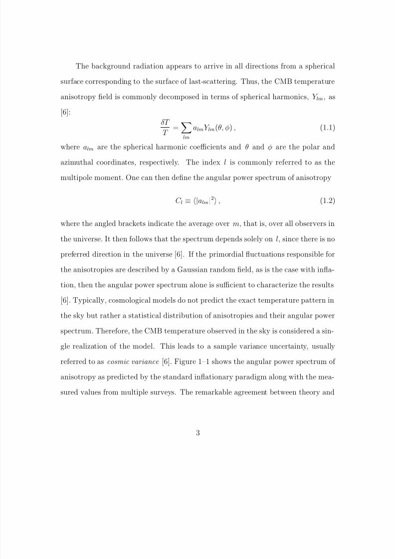
The background radiation appears to arrive in all directions from a spherical
surface corresponding to the surface of last-scattering. Thus, the CMB temperature
anisotropy field is commonly decomposed in terms of spherical harmonics, Y lm, as
[6]:
δT
T =lm
almY lm(θ, φ) , (1.1)
where alm are the spherical harmonic coefficients and θ and φ are the polar and
azimuthal coordinates, respectively. The index l is commonly referred to as the
multipole moment. One can then define the angular power spectrum of anisotropy
C l ≡ |alm|2 , (1.2)
where the angled brackets indicate the average over m, that is, over all observers in
the universe. It then follows that the spectrum depends solely on l, since there is no
preferred direction in the universe [6]. If the primordial fluctuations responsible for
the anisotropies are described by a Gaussian random field, as is the case with infla-
tion, then the angular power spectrum alone is sufficient to characterize the results
[6]. Typically, cosmological models do not predict the exact temperature pattern in
the sky but rather a statistical distribution of anisotropies and their angular power
spectrum. Therefore, the CMB temperature observed in the sky is considered a sin-
gle realization of the model. This leads to a sample variance uncertainty, usually
referred to as cosmic variance [6]. Figure 1–1 shows the angular power spectrum of
anisotropy as predicted by the standard inflationary paradigm along with the mea-
sured values from multiple surveys. The remarkable agreement between theory and
3

8/3/2019 Andrew Stewart- Constraining cosmological parameters with the cosmic microwave background
http://slidepdf.com/reader/full/andrew-stewart-constraining-cosmological-parameters-with-the-cosmic-microwave 13/93
Figure 1–1: The WMAP 5-year TT power spectrum along with recent results fromthe ACBAR [10] (purple), Boomerang [11] (green), and CBI [12] (red) experiments.The pink curve is the best-fit ΛCDM model to the WMAP data. [Figure from [8]]
experiment is clear and illustrates the power of the CMB to constrain cosmological
theories.
Efficient computer codes have been written for calculating the CMB anisotropy
spectra up to an arbitrary multipole moment based on a given set of cosmological
parameters and desired physical effects. The most popular of these codes are cmb-
fast [13] and camb [14], the latter of which is based on the former, with both in
wide use in the physics community. The details of how these codes are implemented
are outside the scope of this work, though we note that these programs can compute
4

8/3/2019 Andrew Stewart- Constraining cosmological parameters with the cosmic microwave background
http://slidepdf.com/reader/full/andrew-stewart-constraining-cosmological-parameters-with-the-cosmic-microwave 14/93
the angular power spectrum in a matter of minutes on a typical desktop computer
to very high accuracy (∼ 0.1% for camb).
In this thesis, we investigate the constraints which can by applied on two different
cosmological parameters using the CMB. In the first part of this work, we develop an
edge detection method of searching CMB temperature anisotropy maps for the effects
of cosmic strings, and we examine how it could be used to constrain the cosmic string
tension. In the second part of this work, using the alternate cosmological model string
gas cosmology as a motivation, we study how well the angular power spectrum of the
CMB can constrain the possible blue tilt of the power spectrum of tensor fluctuations,and how it compares to the constraints applied by other observations. We end with a
review and discussion of the main results emerging from each of these investigations.
5

8/3/2019 Andrew Stewart- Constraining cosmological parameters with the cosmic microwave background
http://slidepdf.com/reader/full/andrew-stewart-constraining-cosmological-parameters-with-the-cosmic-microwave 15/93
CHAPTER 2
Constraint on the Cosmic String Tension
2.1 Overview
At very early times it is believed that the universe underwent a series of symme-
try breaking phase transitions which led to the formation of different types of topo-
logical defects. Among them are linear topological defects know as cosmic strings
[15, 16]. In some scenarios, these defects are stable and can survive until later times.
Topologically stable cosmic strings do not have endpoints and must either extend to
infinity or form closed loops. The quantity which characterizes these cosmic strings
is their tension, µ, which is equivalent to the mass per unit length of the string.
The tension of the cosmic strings is directly determined by the energy scale of the
symmetry breaking during which they were formed, meaning they carry enormous
amounts of energy. It is possible that cosmic strings could have been formed at a
grand unification transition, or later during an electroweak transition, or at any point
in between. Thus, the tension of the cosmic strings can take a wide variety of values.
6

8/3/2019 Andrew Stewart- Constraining cosmological parameters with the cosmic microwave background
http://slidepdf.com/reader/full/andrew-stewart-constraining-cosmological-parameters-with-the-cosmic-microwave 16/93
After creation, the cosmic strings form a random network of infinite strings
and closed string loops. Initially the strings are in a very dense environment and
their motion is damped, but as the universe cools this damping diminishes and the
strings move independently of the contents of the universe. Curved string segments
experience an accelerating force that goes like the string tension, and they quickly
develop relativistic speeds. The arrangement of the cosmic string network then
evolves over time through string interactions. In the event that two cosmic strings
cross there are two possible outcomes: they can simply pass through one another,
or they can break at the point where they come into contact and exchange partners.
The latter case is referred to as intercommutation . Numerical calculations indicate
that intercommutation occurs in almost all cases of string crossing [17]. Of course,
strings can also have self-interactions in which they cross themselves somewhere
along their length. In this case, intercommutation causes the formation of a closed
loop that breaks off of the longer segment. When formed, cosmic string loops are
essentially free from the rest of the network and they continue to oscillate, losing
energy via gravitational radiation, until eventually decaying. Infinitely long strings,
on the other hand, cannot decay into gravitational radiation and survive indefinitely.
Without a mechanism for the string network to lose energy density, cosmic
strings would rapidly come to dominate the universe because they would scale as
non-relativistic matter [15]. Therefore, this transfer of energy density into gravity
waves through the formation of loops is crucial. In conjunction with this energy loss
mechanism, it is expected that the string network eventually approaches a scaling
regime in which the number of strings crossing a given horizon volume is fixed in
7
8/3/2019 Andrew Stewart- Constraining cosmological parameters with the cosmic microwave background
http://slidepdf.com/reader/full/andrew-stewart-constraining-cosmological-parameters-with-the-cosmic-microwave 17/93
such a way that the energy density in cosmic strings scales like radiation [15]. In this
regime, the strings then contribute some fraction of the total energy. The existence
of a scaling solution is supported by numerical simulations of the evolution of the
cosmic string network [18, 19, 20].
When discussing cosmic strings it is common to work with the dimensionless
parameter Gµ, where G is Newton’s constant. The quantity Gµ is of interest be-
cause it characterizes the strength of the gravitational interaction of the strings.
The gravitational perturbations produced by the strings, and thus the density per-
turbations and the induced fluctuations in the CMB, are all of the order of Gµ [15].Until the late 1990’s, cosmic strings were studied as potential seeds for structure
formation [21], fuelled in part by the realization that the density fluctuation from
a string formed around the grand unified epoch would be of the same order as the
temperature anisotropy discovered by COBE [5]. As mentioned in the Introduction,
acoustic peaks were eventually discovered in the CMB angular power spectrum and
subsequently measured with great accuracy. This lead to cosmic strings being ruled
out as the main origin of structure in favour of the inflationary paradigm, since the
angular power spectrum predicted by cosmic strings consists of only a single broad
peak. Despite this, cosmic strings can still contribute partially to the CMB angular
power spectrum (less than 10% [22, 23]). Therefore, there still exists a great deal of
interest in cosmic strings since there are many cosmological models in which their
formation is generically predicted (see [24, 25, 26] for just a few possibilities).
The observational signatures of cosmic strings are distinct and lie within ob-
servational reach. The current bounds on the string tension come from a variety of
8
8/3/2019 Andrew Stewart- Constraining cosmological parameters with the cosmic microwave background
http://slidepdf.com/reader/full/andrew-stewart-constraining-cosmological-parameters-with-the-cosmic-microwave 18/93
measurements. For instance, the gravitational waves emanating from many string
loops at different times produce a stochastic background which is the focus of current
interferometer and pulsar timing experiments. Pulsar timing, specifically, places a
bound Gµ < 10−7−10−8 on the cosmic string tension [27, 28]. However, we note that
in order to place a bound on Gµ using gravitational wave constraints one must make
assumptions about the size of the loops which are formed in the string network, the
probability that strings will intercommute when crossing, and even the string model
under consideration. Therefore, the strength of these bounds can be questioned. As
well as gravitational wave constraints, there is also a bound on the tension coming
from the angular power spectrum of the CMB. As mentioned above, the shape of
the spectrum from cosmic strings alone does not match the observed acoustic peak
structure, meaning they can only contribute a fraction of the cosmological fluctua-
tions. Some work has been devoted to finding the size of this string contribution,
the results of which translate directly into a bound Gµ < 5 × 10⁻⁷ [29, 30].
While the above phenomena can be used to place indirect constraints on the
cosmic string tension there is another observational signature unique to cosmic strings
which could be directly detected, namely, linear discontinuities in the temperature
of the CMB. This signature was first studied by Kaiser and Stebbins [31], and is
commonly referred to as the KS-effect. This effect occurs because the space-time
around a straight cosmic string is flat, but with a wedge, whose vertex lies along
the length of the string, removed. The angle subtended by the missing wedge, φ, is
9
8/3/2019 Andrew Stewart- Constraining cosmological parameters with the cosmic microwave background
http://slidepdf.com/reader/full/andrew-stewart-constraining-cosmological-parameters-with-the-cosmic-microwave 19/93
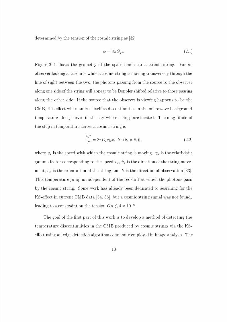
determined by the tension of the cosmic string as [32]
φ = 8πGµ. (2.1)
Figure 2–1 shows the geometry of the space-time near a cosmic string. For an
observer looking at a source while a cosmic string is moving transversely through the
line of sight between the two, the photons passing from the source to the observer
along one side of the string will appear to be Doppler shifted relative to those passing
along the other side. If the source that the observer is viewing happens to be the
CMB, this effect will manifest itself as discontinuities in the microwave background
temperature along curves in the sky where strings are located. The magnitude of
the step in temperature across a cosmic string is
δT
T = 8πGµγ svs |k · (vs × es)| , (2.2)
where vs is the speed with which the cosmic string is moving, γ s is the relativistic
gamma factor corresponding to the speed vs, vs is the direction of the string move-
ment, es is the orientation of the string and k is the direction of observation [33].
This temperature jump is independent of the redshift at which the photons pass
by the cosmic string. Some work has already been dedicated to searching for the
KS-effect in current CMB data [34, 35], but a cosmic string signal was not found,
leading to a constraint on the tension Gµ 4 × 10⁻⁶.
The goal of the first part of this work is to develop a method of detecting the
temperature discontinuities in the CMB produced by cosmic strings via the KS-
effect using an edge detection algorithm commonly employed in image analysis. The
10

8/3/2019 Andrew Stewart- Constraining cosmological parameters with the cosmic microwave background
http://slidepdf.com/reader/full/andrew-stewart-constraining-cosmological-parameters-with-the-cosmic-microwave 20/93
Source Observer
String
Figure 2–1: The geometry of the space-time near a cosmic string. Shown here is aslice of the space-time perpendicular to the orientation of the string. The coloured
area represents a missing wedge with deficit angle φ, while the dashed lines representthe paths of photons travelling from a source to an observer, and the arrow showsthe direction of motion of the string. The photons passing on one side of the cosmicstring will appear to be Doppler shifted with respect to those passing on the otherside due to this non-trivial geometry.
motivation behind this choice is clear since the cosmic strings literally appear as
edges in the CMB temperature. Depending on the sensitivity of the edge detection
algorithm to these temperature edges, we can then place a bound on the cosmic string
tension through Equation (2.2). We expect the bounds arising from this method to
be more robust than those coming from gravitational waves since we do not need to
make assumptions about the nature of the cosmic string network. This work is a
continuation of the study presented in [36].
We are interested in the cosmic strings in the network that survive until later
times, specifically, the times relevant to the production of an edge signature in the
CMB, that is, the time of last scattering until the present time. Based on the
evolution of the network, cosmic strings are more numerous around the time of last
11

8/3/2019 Andrew Stewart- Constraining cosmological parameters with the cosmic microwave background
http://slidepdf.com/reader/full/andrew-stewart-constraining-cosmological-parameters-with-the-cosmic-microwave 21/93
scattering than later times. On today’s sky, those strings correspond to an angular
scale of approximately 1 . Therefore, an observation of the CMB with an angular
resolution substantially less than 1
is necessary in order to be able to detect the
edges related to these strings. With this in mind, we also focus on the application
of the edge detection method to high resolution surveys of the CMB, in particular
the future data from the South Pole Telescope project.
The South Pole Telescope (SPT) [37] is a 10m diameter telescope being deployed
at the South Pole research station. The telescope is designed to perform large area,
high resolution surveys of the CMB to map the anisotropies. The telescope is de-signed to provide 1′ resolution in the maps of the CMB. This makes the SPT ideal
to search for the KS-effect (even better than Planck), and we believe that with such
high resolution data our method could provide bounds on the cosmic string tension
competitive with those of pulsar timing.
The remainder of this chapter is arranged as follows: In section 2.2, we discuss
the simulated CMB maps used in our analysis with a focus on the anisotropies
coming from Gaussian fluctuations and cosmic strings. In Section 2.3, we outline
the edge detection algorithm we are using, highlighting the details of our particular
implementation. In Section 2.4, we discuss how we quantify the edge maps that are
output by the edge detection algorithm. In Section 2.5, we explain the statistical
analysis used to determine if a significant difference has been detected. In Section
2.6, we present the results of running the edge detection algorithm on simulated
CMB maps and the possible constraints on the cosmic string tension that could be
applied. Finally, in Section 2.7, we discuss our results.
12
8/3/2019 Andrew Stewart- Constraining cosmological parameters with the cosmic microwave background
http://slidepdf.com/reader/full/andrew-stewart-constraining-cosmological-parameters-with-the-cosmic-microwave 22/93
2.2 Map Making
To use an edge detection algorithm to search for a cosmic string signal we first
need an image, or map, to run it on. For this initial investigation of edge detection
as a method for constraining or even detecting cosmic strings, we generate CMB
temperature anisotropy maps by means of numerical simulations and use these as the
input for the edge detection algorithm. By utilizing numerical simulations, we know
exactly the parameters used to generate each temperature anisotropy map. That way,
when we compare the output of the edge detection algorithm for different input maps,
we can conclude if the method is able to make a significant discrimination or not. If
edge detection proves to be a feasible method for detecting a string signal, the goal is
to eventually examine real CMB data for the presence of cosmic strings. To do so, we
would first need to compute an idealized set of data corresponding to the appropriate
cosmological theory and compare it to what is found in the real microwave sky. This
presents us with another reason to develop a method of generating simulated CMB
maps.
The simulated maps are constructed through the superposition of different tem-
perature anisotropy components based on the type of effects being reproduced. We
are interested in the simulation of small angular scale patches of the microwave sky,
so we employ the flat-sky approximation [38]. In this approximation, the geometry
of a small patch on the sky can be considered to be essentially flat. Thus, each
map component, as well as the final map itself, is a two dimensional square image
characterized by an angular size and an angular resolution. Specifically, we work
13

8/3/2019 Andrew Stewart- Constraining cosmological parameters with the cosmic microwave background
http://slidepdf.com/reader/full/andrew-stewart-constraining-cosmological-parameters-with-the-cosmic-microwave 23/93
with a square grid that has a size corresponding to the angular size being simulated,
and a pixel size corresponding to the angular resolution being simulated. The pixels
in the grid are indexed by two dimensional Cartesian coordinates (x, y) and we take
the upper left corner of the grid to be the origin.
The common component in every simulated CMB map is a set of temperature
anisotropies produced by Gaussian inflationary fluctuations. The normal distribution
of these fluctuations is predicted by various cosmological models and is supported
by current observations [7]. These fluctuations must be included because they cor-
respond to an angular power spectrum like that measured in the real microwave sky[7]. In fact, we simulate the Gaussian fluctuations such that they account for all of
the observed power in the CMB. Thus, in the absence of any other effects the final
simulated map is simply equivalent to the Gaussian component and is consistent
with observations. That is, we define
T (x, y) ≡ T G(x, y) , (2.3)
where T (x, y) represents the the final temperature anisotropy map and T G(x, y) rep-
resents the Gaussian component. We signify the maps by T simply as a choice of
notation, but we note that the value of each pixel is actually that of the temperature
anisotropy δT/T .
To make a CMB map including the effects of cosmic strings, we simulate a
separate component of string induced temperature fluctuations produced via the
KS-effect. The final temperature anisotropy map is then given by a combination of
the string and Gaussian components. Denoting the string component by T S (x, y),
14
8/3/2019 Andrew Stewart- Constraining cosmological parameters with the cosmic microwave background
http://slidepdf.com/reader/full/andrew-stewart-constraining-cosmological-parameters-with-the-cosmic-microwave 24/93
we define the final temperature as
T (x, y)
≡α T G(x, y) + T S (x, y) , (2.4)
where α is a scaling factor which depends on the tension of the cosmic strings in
T S (x, y). We must scale the amplitude of the Gaussian component to compensate for
the excess power we introduce by adding a component of string-induced fluctuations.
In this way the strings can contribute a fraction of the total power, while the final
map is still in agreement with current CMB survey results.
Let us comment in more detail on the nature of this scaling. We demand that theangular power of the final combined temperature map match the observed angular
power for multipole values up to the first acoustic peak, i.e. l 220. We choose
this multipole range because it is tightly constrained by current observations [7].
Then again, as mentioned above, the Gaussian component alone accounts for all
of the observed angular power in the CMB. Thus, this demand is equivalent to
requiring that the angular power of the combined map match that of a pure Gaussian
component. Working in the flat-sky approximation allows us to replace the usual
spherical harmonic analysis of the CMB fluctuations by a Fourier analysis [38]. We
can then express our condition as
|T G(k < k p)|2 = α2|T G(k < k p)|2 + |T S (k < k p)|2 , (2.5)
where k p is the wavenumber corresponding to the first acoustic peak of the angular
power spectrum of the CMB, |T S (k < k p)|2 is the average of the Fourier tempera-
ture anisotropy values from the string component for wavenumbers less than k p and
15

8/3/2019 Andrew Stewart- Constraining cosmological parameters with the cosmic microwave background
http://slidepdf.com/reader/full/andrew-stewart-constraining-cosmological-parameters-with-the-cosmic-microwave 25/93
|T G(k < k p)|2 is the equivalent object for the Gaussian component. From Equation
(2.2) one can see that the average of the temperature anisotropy values in the string
component should go as the cosmic string tension squared. Therefore, if we define a
reference cosmic string tension, Gµ0, we have
|T S (k < k p)|2 = |T S (k < k p)|20
Gµ
Gµ0
2
, (2.6)
where |T S (k < k p)|20 is the average for a string component corresponding to the
reference tension and Gµ is the cosmic string tension corresponding to the string
component on the left-hand side of the equation. Substituting this into (2.5) we can
solve for the final form of the scaling factor:
α2 = 1 − |T S (k < k p)|20|T G(k < k p)|2
Gµ
Gµ0
2
. (2.7)
The benefit of having α in this form is we need only calculate the ratio of averages
once using the reference tension. After this we can calculate the value of the scaling
factor with only the cosmic string tension used in the given simulation, Gµ. More
detailed studies of combining string anisotropies and Gaussian anisotropies have
concluded that, in general, a cosmic string contribution of less than 10% of the
observed CMB power on large scales cannot be ruled out [22, 23].
A third component which we can include in the final map is a simulation of
instrumental noise. Any real CMB survey has some amount of noise associated with
its observation and we add this component to examine the effect that noise has on
the ability of an edge detection algorithm to detect a cosmic string signal. As a crude
approximation, we simulate an instrumental noise component that is simply white
16

8/3/2019 Andrew Stewart- Constraining cosmological parameters with the cosmic microwave background
http://slidepdf.com/reader/full/andrew-stewart-constraining-cosmological-parameters-with-the-cosmic-microwave 26/93
noise with some given maximum amplitude in the temperature difference δT N,max.
If an instrumental noise component is included we do not need to perform any addi-
tional scaling since it is an unphysical effect, and it is simply summed directly to the
other components. Therefore, denoting the noise component by T N (x, y), we have
T (x, y) ≡ T G(x, y) + T N (x, y) (2.8)
for a simulation without cosmic strings, or
T (x, y) ≡ α T G(x, y) + T S (x, y) + T N (x, y) (2.9)
for a simulation including cosmic strings.
The dominant portion of the final simulated map is the Gaussian temperature
fluctuations. As such, these Gaussian fluctuations represent the most significant
“noise” when trying to directly detect the effect of cosmic strings with the edge
detection algorithm. The significance of the instrumental noise component in the
final map is determined by the maximum amplitude of the noise, which should in
general be small compared to the amplitude of the Gaussian fluctuations. The size
of the temperature anisotropies in the string component depends directly on the
tension of the cosmic strings which are being simulated, as described by Equation
(2.2). For sensible values of the string tension, the amplitude of the string-induced
anisotropies will lie from a factor of a few up to orders of magnitude below the
amplitude of the Gaussian temperature anisotropies, thus presenting the difficulty
in directly detecting them.
17

8/3/2019 Andrew Stewart- Constraining cosmological parameters with the cosmic microwave background
http://slidepdf.com/reader/full/andrew-stewart-constraining-cosmological-parameters-with-the-cosmic-microwave 27/93
The simulation of an entire CMB temperature anisotropy map is not particularly
resource intensive and typically takes of the order of a few minutes on a standard
desktop computer, depending on the angular resolution and angular size of the sim-
ulated survey and on which components are being included.
Before moving on to discuss the edge detection algorithm itself, we first review
our methods for generating the Gaussian and string components since they contain
all of the interesting physics.
2.2.1 The Gaussian Component
In this section we discuss in more detail the actual numerical simulation of the
Gaussian temperature fluctuations. The free parameters in the simulation of the
Gaussian component are the angular resolution and the angular scale.
As touched on above, the spherical harmonic expansion of the CMB temperature
anisotropies, as given in equation (1.1), can be replaced by a Fourier expansion when
using the flat-sky approximation [38]. Therefore, when generating the component of
Gaussian fluctuations, we choose to work on a grid in Fourier space. In this case, each
pixel in the grid is indexed by the coordinates (kx, ky), which are the components
of the wavevector pointing to that pixel. The size and resolution of the grid still
correspond to the two angular scales in the simulation. The advantage of being able
to use a Fourier analysis is that it greatly simplifies the calculations, and the value
of the temperature anisotropy at a particular pixel on the the grid is then given by
18
8/3/2019 Andrew Stewart- Constraining cosmological parameters with the cosmic microwave background
http://slidepdf.com/reader/full/andrew-stewart-constraining-cosmological-parameters-with-the-cosmic-microwave 28/93
the relation
δT GT
(kx, ky) = g(kx, ky) a(kx, ky) , (2.10)
where g(kx, ky) is a random number taken from a normal probability distribution
with mean zero and variance one [39]. The quantity a(kx, ky) is the Fourier space
equivalent of alm in (1.1) and is related to the angular power spectrum of the tem-
perature anisotropy in the same way,
< |a(kx, ky)|2 >= C l . (2.11)
In the flat-sky approximation the multipole moment is related to pixel position inthe grid by
l =2π
θ
k2x + k2
y , (2.12)
where θ is the angular size of the survey area [39].
When performing the numerical simulation, we first compute the COBE normal-
ized angular power spectrum up to the required multipole moment using the camb
software. One can see from Equation (2.12) that, in general, the largest multipole
moment required for a simulation increases as the resolution increases. Therefore,
since we are interested in simulating high resolution CMB maps, we require the
values of the angular power spectrum at very large multipole moments. There are
currently no CMB surveys taking measurement up to the l-values needed in our
simulated maps, so we run camb with input cosmological parameters determined
by surveys at lower angular resolution. To be precise, when computing the angular
power spectrum with camb, we choose our input parameters to be those derived
19

8/3/2019 Andrew Stewart- Constraining cosmological parameters with the cosmic microwave background
http://slidepdf.com/reader/full/andrew-stewart-constraining-cosmological-parameters-with-the-cosmic-microwave 29/93
using the CMBall data set, which combines the results from multiple surveys [10].
We stress, however, that we are free to choose any particular set of parameters we
like.
The next step is to compute the temperature fluctuations pixel by pixel using
the angular power spectrum output by camb. For each pixel (kx, ky) we compute
the corresponding multipole moment using Equation (2.12). Clearly though, l can
take non-integer values, whereas the angular power spectrum is computed for only
integer values. Therefore, we approximate the value of the angular power spectrum
at l using the linear interpolation
C l = C lb + (l − lb)(C la − C lb) , (2.13)
where la is the integer value lying above l and lb is the integer value lying below.
With the value of the angular power spectrum at (kx, ky), it is then straightforward
to calculate the Fourier temperature anisotropy value using Equations (2.11) and
(2.10). Once we have computed the value of each pixel in the grid we take the inverse
Fourier transform of the array using a fast Fourier transform (FFT) algorithm. This
produces a temperature anisotropy map in position space.
By choosing the origin of the grid to be at the top left corner, we have introduced
a preferred direction into the simulation of the Gaussian fluctuations. To compensate
for this asymmetry we construct the final Gaussian component, T G(x, y), by superim-
posing four separate sub-components, which we label as T 1...T 4, each computed sep-
arately using the method described above. When combining these sub-components
we reflect each along one of the four axes on the grid. In this way, we eliminate any
20
8/3/2019 Andrew Stewart- Constraining cosmological parameters with the cosmic microwave background
http://slidepdf.com/reader/full/andrew-stewart-constraining-cosmological-parameters-with-the-cosmic-microwave 30/93
irregularity in the final map. Therefore, the Gaussian component is defined as
T G(x, y)
≡
1
2T 1(x, y) + T 2(xmax
−x, y)
+T 3(x, ymax − y) + T 4(xmax − x, ymax − y)
, (2.14)
where xmax and ymax are the maximal x and y values based on the simulation pa-
rameters. The factor of 1/2 in front of the sum is required to maintain the original
standard deviation.
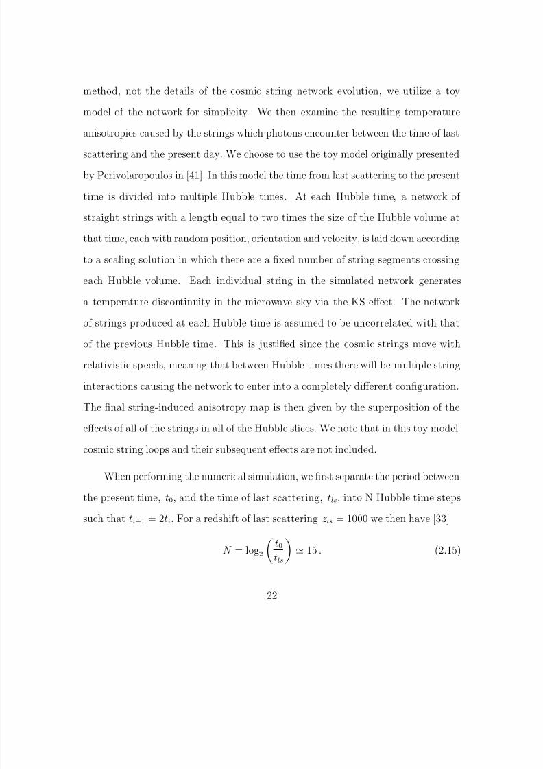
Figure 2–2 shows a Gaussian component produced using the method described
above. One can see the familiar smooth regions of positive and negative deviations
from the background temperature, present in all maps of the CMB. The amplitude
of the fluctuations are of the order of 10−5 matching those measured in the real
microwave sky [5]. We also note that there is no evidence of a preferred direction in
the final map component.
2.2.2 The String Component
As with the Gaussian component, in this section we discuss the details of the
numerical simulation of the string component. The free parameters in the simulation
of the string component are the angular resolution, the angular scale, the cosmic
string tension and the number of cosmic strings per Hubble volume.
Detailed numerical simulations of cosmic string networks have been performed
for a number of years and as a whole share the trait of being very computationally
intensive [18, 19, 20, 40]. Since the focus of this work is on testing the edge detection
21
8/3/2019 Andrew Stewart- Constraining cosmological parameters with the cosmic microwave background
http://slidepdf.com/reader/full/andrew-stewart-constraining-cosmological-parameters-with-the-cosmic-microwave 31/93
method, not the details of the cosmic string network evolution, we utilize a toy
model of the network for simplicity. We then examine the resulting temperature
anisotropies caused by the strings which photons encounter between the time of last
scattering and the present day. We choose to use the toy model originally presented
by Perivolaropoulos in [41]. In this model the time from last scattering to the present
time is divided into multiple Hubble times. At each Hubble time, a network of
straight strings with a length equal to two times the size of the Hubble volume at
that time, each with random position, orientation and velocity, is laid down according
to a scaling solution in which there are a fixed number of string segments crossing
each Hubble volume. Each individual string in the simulated network generates
a temperature discontinuity in the microwave sky via the KS-effect. The network
of strings produced at each Hubble time is assumed to be uncorrelated with that
of the previous Hubble time. This is justified since the cosmic strings move with
relativistic speeds, meaning that between Hubble times there will be multiple string
interactions causing the network to enter into a completely different configuration.
The final string-induced anisotropy map is then given by the superposition of the
effects of all of the strings in all of the Hubble slices. We note that in this toy model
cosmic string loops and their subsequent effects are not included.
When performing the numerical simulation, we first separate the period between
the present time, t0, and the time of last scattering, tls, into N Hubble time steps
such that ti+1 = 2ti. For a redshift of last scattering zls = 1000 we then have [33]
N = log2
t0tls
≃ 15 . (2.15)
22

8/3/2019 Andrew Stewart- Constraining cosmological parameters with the cosmic microwave background
http://slidepdf.com/reader/full/andrew-stewart-constraining-cosmological-parameters-with-the-cosmic-microwave 32/93
For large redshifts and assuming Ω0 = 1, the angular size of the Hubble volume
at a given Hubble time is approximated by θH i ∼ z−1/2i ∼ t
1/3i . Therefore, we have
θH ls ≃ z−1/2
ls ≃ 1.8
for the Hubble volume corresponding to the time of last scattering
and θH i+1 ≃ 21/3θH i for all subsequent Hubble time steps [33]. We calculate the
contribution to the final temperature anisotropy map from each of the Hubble slices
separately. For a specific Hubble time step ti we start with an extended region that
has a total angular size equivalent to the angular size of the string component being
simulated plus two times the angular size of the Hubble volume at that particular
Hubble time. The number of strings ni that should exist in that particular region is
then given by the scaling solution
ni = M (θ + 2θH i)
2
θ2H i
, (2.16)
where M is the number of cosmic strings crossing each Hubble volume and θ is the
angular size of the string component being simulated [33]. As usual, we work on a
square grid, this time placed over the entire extended region, with pixel size given
by the angular resolution being considered.
Pixels within the entire extended area are then chosen at random to be the
midpoints of strings, with a probability such that the average number of strings in a
single Hubble volume is in agreement with the number M of the scaling solution. If
a pixel is chosen to be a midpoint, we choose a random orientation about that pixel
and we place a straight string of length 2θH i . We then simulate the temperature
23

8/3/2019 Andrew Stewart- Constraining cosmological parameters with the cosmic microwave background
http://slidepdf.com/reader/full/andrew-stewart-constraining-cosmological-parameters-with-the-cosmic-microwave 33/93
fluctuation produced by that string by adding a temperature anisotropy
δT S
T
= 4πGµγ svsr (2.17)
to a rectangular region on one side of the string, and subtracting the same amount
from a rectangular region on the other side. This temperature anisotropy corresponds
to the KS-effect as given by Equation (2.2), where r = |k ·(vs× es)| takes into account
the projection effects. The direction of observation k is approximately constant over
the entire field of view while the quantity vs × es is a random unit vector since both
the string orientation and velocity are random. Thus, the value of r is uniformly
distributed over the interval [0,1] [33]. In Equation (2.17), we take the RMS speed
of the strings to be vs = 0.15 [33], so the amplitude of the fluctuation is determined
entirely by the string’s tension and its orientation. Each rectangular region affected
by the temperature fluctuation has a length 2θH i along the direction of the string and
extends a distance θH i in the direction perpendicular to the string. Thus, each cosmic
string gives rise to five separate temperature discontinuities: one at its position, two
parallel to it at a distance θH i and two perpendicular to the string at the endpoints.
After placing all of the cosmic strings and calculating the temperature fluctuation
for each, we have finished simulating the cosmic string network for the given Hubble
time step.
Since we began with a region which is larger than the string component we
wanted to simulate in the first place, we must crop the larger area to the correct size.
We choose to discard pixels equally from all four sides of the extended area, so that
we retain only those from the central region of the larger area. By identifying the
24

8/3/2019 Andrew Stewart- Constraining cosmological parameters with the cosmic microwave background
http://slidepdf.com/reader/full/andrew-stewart-constraining-cosmological-parameters-with-the-cosmic-microwave 34/93
correctly sized simulated area with the centre of the extended area, one can see that
what we essentially did when first defining the extended region was to enlarge the
actual simulation area by a Hubble volume in each direction. The reason that we
expand our simulated area in this way is because any string whose midpoint is within
a distance θH i of the actual area we want to simulate could enter into it. Thus, we
must also account for these strings which lie around the edges of the area of interest,
not only those centred within it.
Finally, when we have simulated the string network for each Hubble time step,
we sum together these fifteen sub-components pixel by pixel. This superpositionapproximates what the contribution from the entire, more complex cosmic string
network would be, and gives the final cosmic string component, T S (x, y).
In the model described above, we have fixed values for the the speed of the
strings, the length of the strings and the depth of the temperature fluctuation region
around the string. These values were obtained from particular numerical simulations
[33], however, these parameters can vary significantly for different models of the
string network (see [16] for a review) and should not be considered as established.
Figure 2–2 shows a cosmic string component simulated using the model described
above. Clearly visible are the sharp temperature discontinuities caused by individual
straight strings as well as the cumulative effect of the entire cosmic string network.
The amplitude of the fluctuations in the string component are small compared to
those appearing due to Gaussian fluctuations. The random way in which the cosmic
strings are positioned and oriented in the network is also apparent.
25
8/3/2019 Andrew Stewart- Constraining cosmological parameters with the cosmic microwave background
http://slidepdf.com/reader/full/andrew-stewart-constraining-cosmological-parameters-with-the-cosmic-microwave 35/93
4.01e-5 -4.46e-5 1.12e-6 -2.78e-6
Figure 2–2: Components of a simulated temperature anisotropy map. On the leftis an example of a component of Gaussian temperature fluctuations. On the right
is an example of a component of cosmic string induced temperature fluctuations.In both components, the angular size of the simulated region is 2.5 ×2.5 and theangular resolution is 1′ per pixel (22,500 pixels). In the string component the tensionof the cosmic strings was taken to be Gµ = 6 × 10⁻⁸ and the number of strings perHubble volume in the scaling solution was taken to be M = 10. The colour of a pixelrepresents the value of the temperature anisotropy at that pixel, as described by thescale below each image.
26

8/3/2019 Andrew Stewart- Constraining cosmological parameters with the cosmic microwave background
http://slidepdf.com/reader/full/andrew-stewart-constraining-cosmological-parameters-with-the-cosmic-microwave 36/93
2.3 The Canny Edge Detection Algorithm
At this point we are ready to discuss how to run the edge detection algorithm on
one of the simulated CMB anisotropy maps. When looking for edges in an image we
are looking for curves across which there is a strong intensity contrast. The strength
of an edge can then be quantified by the magnitude of the contrast from one side
of the edge to the other, or equivalently, the magnitude of the gradient across the
edge. For CMB temperature anisotropy maps, the intensity that we are dealing with
is simply the amplitude of the fluctuations. Thus, we define the edges in the CMB
maps as lines across which the temperature difference is large.
To search for edges in CMB temperature anisotropy maps we use the Canny edge
detection algorithm. The Canny algorithm is a multi-stage edge detection algorithm
first developed in 1986 by John F. Canny [42]. Despite its age, this algorithm remains
one of the most commonly used edge detection methods in image analysis. Canny’s
goal was to develop an optimal edge detector which combined good detection and
localization of edges without being prone to false detection. He found that, given
his criteria, the ideal edge filter was well approximated by first-order derivatives of
a Gaussian [42]. The benefit of using the Canny algorithm is that it has a relatively
simple and straightforward implementation which also offers a certain amount of
flexibility, allowing us to optimize the procedure for our purpose.
The process of detecting the edges in a temperature anisotropy map using the
Canny algorithm takes of the order of one minute, depending on the angular size and
resolution.
27
8/3/2019 Andrew Stewart- Constraining cosmological parameters with the cosmic microwave background
http://slidepdf.com/reader/full/andrew-stewart-constraining-cosmological-parameters-with-the-cosmic-microwave 37/93
In the following sections we review in detail how we apply the Canny algorithm to
CMB maps to search for edges. The free parameters in the edge detection algorithm
are the size of the gradient filter (the filter length) and the value of the three edge
thresholds.
2.3.1 Non-maximum Suppression
Since we are interested in temperature gradients, the first step of the Canny edge
detection algorithm is to simply compute the gradient of the temperature anisotropy
map and use it to determine which pixels could be part of an edge.
For consistency with the above sections, we denote the input temperature ani-
sotropy map by T (x, y). To compute the gradient of T (x, y) we first construct two
square filters, F x(x, y) and F y(x, y), which are first-order derivatives of a two dimen-
sional Gaussian function along each of the two map coordinates (x, y), respectively.
These filters have the form:
F x(x, y) = − x
2πσ4e−(x2+y2)
2σ (2.18)
F y(x, y) = − y
2πσ4e−(x2+y2)
2σ . (2.19)
We then apply each filter separately at every pixel in the temperature anisotropy map
in order to find the gradient magnitude along each coordinate axis. The components
of the gradient magnitude along the x-direction and y-direction, denoted by Gx and
28

8/3/2019 Andrew Stewart- Constraining cosmological parameters with the cosmic microwave background
http://slidepdf.com/reader/full/andrew-stewart-constraining-cosmological-parameters-with-the-cosmic-microwave 38/93
Gy respectively, are given by
Gx(x, y) = i,j
F x(i, j)T (x + i, y + j) (2.20)
Gy(x, y) =i,j
F y(i, j)T (x + i, y + j) , (2.21)
where the maximum and minimum values of i and j are determined by the filter
length. In practise, we actually compute Gx(x, y) and Gy(x, y) by a convolution of
the temperature map with the filter using a FFT for the sake of increased speed.
With the component of the gradient in each direction known at every pixel, we can
construct a new map
G(x, y) =
G2x(x, y) + G2
y(x, y) , (2.22)
which is the map of the gradient magnitude, or edge strength, corresponding to the
original temperature anisotropy map. We can also construct a second map
θG(x, y) = arctan
Gy(x, y)
Gx(x, y)
, (2.23)
which is the map of the gradient angle, or gradient direction. In the above equation
the sign of both components is taken into account so that the angle is placed in the
correct quadrant. Therefore, the arctangent has a range of (−180 , 180 ].
In the Canny algorithm, part of the definition of a pixel that is considered to be
on an edge is that it must be a local maximum in the gradient magnitude. By local
maximum we mean that the gradient magnitude at a given pixel is larger than that of
both pixels which neighbour it along the axis defined by the gradient direction at thatpixel. Using the gradient magnitude and direction maps, it is straightforward then
29

8/3/2019 Andrew Stewart- Constraining cosmological parameters with the cosmic microwave background
http://slidepdf.com/reader/full/andrew-stewart-constraining-cosmological-parameters-with-the-cosmic-microwave 39/93
to check the local maximum condition pixel by pixel and determine which could be a
part of an edge and which could not be part of an edge. Since we are only interested
in constructing a final map of edges, if a pixel does not satisfy the local maximum
condition we immediately discard that pixel. Therefore, this process is referred to as
non-maximum suppression .
On a square grid there are only eight distinguished directions which form four
axes, namely the two directions along each coordinate axis and the two directions
along each diagonal axis. For the sake of simplicity, when referring to the eight
directions on the grid we make an analogy with the eight directions on the face of acompass (i.e the positive x-direction is equivalent to east, etc.). However, as already
mentioned, the gradient direction as calculated in Equation (2.23) can take any value
(−180 , 180 ]. Thus, in order to relate the gradient direction, or equivalently the edge
direction, to one that we can trace on the grid, we must approximate the value of
θG(x, y) at each pixel to lie along one of the eight grid directions. The definition of
the approximated gradient directions is given in Table 2–1.
For the purpose of performing the non-maximum suppression we first check the
approximated gradient direction at a given pixel to determine which of the four grid
axes corresponds to the gradient axis at that pixel. We then record the gradient
magnitude of the two pixels which neighbour the original pixel along that gradient
axis. For example, if the gradient direction is approximated as north-west then we
record the gradient magnitude of the pixel to the north-west and the pixel to the
south-east. Lastly, we compare the gradient magnitude of the original pixel to the
gradient magnitudes of the two neighbours. Only if the gradient magnitude is larger
30

8/3/2019 Andrew Stewart- Constraining cosmological parameters with the cosmic microwave background
http://slidepdf.com/reader/full/andrew-stewart-constraining-cosmological-parameters-with-the-cosmic-microwave 40/93
Table 2–1: Definition of the approximate gradient directions used in the edge detec-tion algorithm. In the left column are the different ranges of values that the gradientdirection can take. In the right column are the approximated gradient directionsmatching each of the eight directions on the grid. Depending on which range a given
pixel falls into in the left column, the gradient direction at that pixel will then bereplaced by the corresponding approximation in the right column.
Actual Gradient Direction Approximated Gradient Direction−22.5 ≤ θG(x, y) < 22.5 θG(x, y) ≃ 0 (east)
22.5 ≤ θG(x, y) < 67.5 θG(x, y) ≃ 45 (north-east)
67.5 ≤ θG(x, y) < 112.5 θG(x, y) ≃ 90 (north)
112.5 ≤ θG(x, y) < 157.5 θG(x, y) ≃ 135 (north-west)
157.5 ≤ θG(x, y) < −157.5 θG(x, y) ≃ 180 (west)
−157.5
≤θG(x, y) <
−112.5 θG(x, y)
≃ −135 (south-west)
−112.5 ≤ θG(x, y) < −67.5 θG(x, y) ≃ −90 (south)
−67.5 ≤ θG(x, y) < −22.5 θG(x, y) ≃ −45 (south-east)
than both neighbours is the pixel considered a local maximum, or possibly part of
an edge.
Figure 2–3 shows a gradient magnitude map after non-maximum suppression
has been performed. To clearly illustrate the result of performing non-maximum
suppression, we present the map of local maxima corresponding to the same cosmic
string component shown in Figure 2–2 with no other components added to it, yet
this does not represent a legitimate final simulated CMB map. Many of the orig-
inal pixels have been discarded, as expected, and we are left with a rough map of
edges. Although curves corresponding to certain edges in the original temperature
anisotropy component can be seen, there are many other pixels marked as local max-
ima corresponding to extremely weak edges, making the signal from stronger edges
difficult to detect.
31

8/3/2019 Andrew Stewart- Constraining cosmological parameters with the cosmic microwave background
http://slidepdf.com/reader/full/andrew-stewart-constraining-cosmological-parameters-with-the-cosmic-microwave 41/93
2.3.2 Thresholding with Hysteresis
The map produced after performing non-maximum suppression represents pixels
which could perhaps be on an edge. Thus, the next step of the Canny algorithm is
to produce the final map of genuine edge pixels from the map of local maxima.
When performing non-maximum suppression we only compared a single pixel
with two of its neighbours to determine if it could be part of an edge. Pixels with
a small gradient magnitude may have still been marked as a local maxima if the
gradient magnitudes of their neighbours were also small. As discussed above, Figure
2–3 shows that this is indeed the case. The magnitude at such pixels can in fact be
so small that we do not want to consider them as edge pixels, since they can dilute
the more significant signal coming from stronger edges. In addition, because we want
to detect edges which appear due to cosmic strings via the KS-effect, we expect the
gradient direction to be consistent across the length of the string induced edge. This
directionality needs to be taken into account to determine which local maxima pixels
belong to the same string edge. Taking these two points into consideration, we must
further expand our definition of exactly what constitutes an edge pixel.
The Canny algorithm outlines a process of applying multiple thresholds to define
the edges in an image, known as thresholding with hysteresis. First, we choose an
upper gradient threshold, tu < 1, such that we can then define a pixel which is
definitely part of an edge, which we name a true-edge pixel , as one which is not only
a local maximum but also satisfies
G(x, y) ≥ tuGm . (2.24)
32

8/3/2019 Andrew Stewart- Constraining cosmological parameters with the cosmic microwave background
http://slidepdf.com/reader/full/andrew-stewart-constraining-cosmological-parameters-with-the-cosmic-microwave 42/93
Here Gm is the mean maximum gradient magnitude computed from simulated tem-
perature maps which contain only strings. The value of Gm depends on the param-
eters of the simulation being performed, most notably the string tension, and must
be computed separately for each parameter set using a selected number of simulated
string maps. One can think of Gm as representing the strongest possible edge that
could be formed by cosmic strings alone. Therefore, with this threshold, we are sim-
ply stating that if the gradient magnitude at a given pixel is some chosen fraction of
the maximum possible, then it must be a true-edge pixel.
It is not sufficient, however, to define the edges using only one threshold becausethe gradient magnitude can fluctuate at each pixel along the length of an edge. This
variation can be caused by both instrumental noise and the random nature of the
Gaussian anisotropies. If we applied only an upper threshold, we would reject the
pixels at which the gradient magnitude fluctuates below that threshold, but should in
fact still be considered as a part of a given edge. This would lead to edges being cut
into smaller segments, making them look like dashed lines, rather than continuous
curves on the map. To avoid this, we also choose a lower gradient threshold, tl < tu,
and define a pixel which is possibly part of an edge, which we name a semi-edge
pixel , as a local maximum pixel satisfying
tlGm ≤ G(x, y) < tuGm . (2.25)
We then further assert that any semi-edge pixel which is in contact with a true-
edge pixel and has the appropriate gradient directionality is also a true-edge pixel
sharing the same edge (see the later discussion in this section for a full explanation
33
8/3/2019 Andrew Stewart- Constraining cosmological parameters with the cosmic microwave background
http://slidepdf.com/reader/full/andrew-stewart-constraining-cosmological-parameters-with-the-cosmic-microwave 43/93
of these conditions). This allows us to fill the gaps between true-edge pixels and
avoid incorrect breaking up of the edges. If a semi-edge pixel is not in contact with
a true-edge pixel, then it is rejected. If a local maximum pixel still falls below the
lower threshold then it is also rejected. The latter case is the requirement that an
edge pixel have some minimum strength, and cures the problem of a local maxima
with extremely small gradient magnitudes being included in the final edge map.
Since we are interested in edges appearing due of the presence of cosmic strings,
we also apply a “cutoff” threshold such that we reject all pixels for which
G(x, y) > tcGm , (2.26)
where tc ≥ 1. We apply this third threshold because the Gaussian temperature
fluctuations in the CMB map dominate those coming from the cosmic strings. As
such, they lead to edges with much stronger gradient magnitudes, that is, greater
than Gm. If we only applied the upper bound tu, these edges would overwhelm the
edge detection algorithm, washing out the cosmic string signal. By setting a cutoff
threshold, we can discard the pixels with a gradient magnitude which we consider to
be too strong to have been caused by cosmic strings, and keep only those representing
the cosmic string signature. We choose tc ≥ 1 because we also consider the slight
enhancement of weak edges corresponding to Gaussian fluctuations, as a result of
the underlying cosmic string edges, to be part of the cosmic string signal.
To perform the final edge detection on the map of local maxima we first apply the
thresholds as described above. After applying the thresholds we no longer need the
information about the gradient magnitude. Thus, we introduce a simplified notation
34

8/3/2019 Andrew Stewart- Constraining cosmological parameters with the cosmic microwave background
http://slidepdf.com/reader/full/andrew-stewart-constraining-cosmological-parameters-with-the-cosmic-microwave 44/93
in which we mark true-edge pixels as 1, semi-edge pixels as 1/2 and all rejected pixels
as 0.
We then check which semi-edge pixels are actually true-edge pixels. We begin
by searching the map for a pixel which is a 1 and has not already been examined
during the tracing of a different edge. If we find one we then check the gradient
direction at that pixel to determine the axis along which the gradient lies. Given the
gradient axis, we inspect each of the six neighbouring pixels which do not lie along
that axis for ones which are non-zero. For example, if the gradient lies along the
north-south axis then we would check the pixels to the north-west, west, south-west,south-east, east and north-east. The two directions perpendicular to the gradient
axis represent the edge axis while the other four directions represent the two axes
which are next to parallel to the edge axis. The reason that we look at the neighbours
along six directions, rather than only the two directions along the edge, is because
we are working on a grid with finite resolution. As such, a wiggle in a real string,
which occurs on a scale below the grid resolution, may manifest itself in the map
as an abrupt jump in the edge position from one pixel to the next. Even a straight
string, depending on its orientation, may appear to have one or more “steps” when
it is viewed at the resolution of the grid. Thus, we cannot expect an edge to be a
continuous chain with the next edge pixel always lying along the edge axis defined
by previous pixel. If we did not account for this, it could lead to the tracing of edges
being prematurely terminated, causing an overabundance of short edges.
If any of the six neighbouring pixels is marked as 1/2 we check the gradient
direction at that pixel. If the gradient direction is parallel or next to parallel to
35
8/3/2019 Andrew Stewart- Constraining cosmological parameters with the cosmic microwave background
http://slidepdf.com/reader/full/andrew-stewart-constraining-cosmological-parameters-with-the-cosmic-microwave 45/93
the gradient direction at the original pixel, we immediately change the neighbouring
pixel from a 1/2 to a 1, that is, we change it from a semi-edge pixel to a true-edge
pixel. If the gradient direction is not parallel or next to parallel, then we do not
consider the neighbour as part of the same edge and we ignore it. The comparison
of the gradient directions represents our demand that the temperature gradient be
consistent along an entire edge. If any neighbouring pixel is already marked as a 1
and has not been examined during the tracing of another edge, then we check the
gradient direction at that pixel. If it is in agreement, in the above sense, with that
of the original pixel, we consider it part of the same edge. Once we have checked all
six neighbours of the original pixel we mark it as having been examined.
If we did find a neighbour which is considered to be an edge pixel on the same
edge, regardless of whether it was originally a 1/2 or a 1, we then move to that pixel
and repeat the process of checking the neighbouring pixels. If that pixel then has
another neighbour sharing the same edge that neighbour will be marked as a 1 (if
necessary) and we move to that pixel, and so on. The process of moving pixel by
pixel continues until we reach a pixel that has no neighbours considered to be sharing
the same edge. In this way we will eventually trace the entire edge.
We note two additional points related to tracing the edges in the map. Clearly
when we move to a neighbouring pixel the original pixel will then be a neighbour
of that pixel. By keeping track of which pixels have been examined at each step we
know not to move back to the original pixel again and we do not repeat the process
for the same pixels over and over. Secondly, if the original edge pixel is not the
endpoint of an edge, then it should have two neighbours which share the same edge.
36

8/3/2019 Andrew Stewart- Constraining cosmological parameters with the cosmic microwave background
http://slidepdf.com/reader/full/andrew-stewart-constraining-cosmological-parameters-with-the-cosmic-microwave 46/93
If this is the case we mark both as true-edge pixels (if necessary) and then check the
neighbours of each of those pixels separately. In this way we trace the edge along two
separate paths simultaneously, but the end result is still a single continuous curve.
The entire process described above traces a single edge in the map. When we
have finished with a particular edge, we then search for the next pixel in the map
which is a 1 and has not already been examined. If we find one, we then start from
that pixel and trace the corresponding edge until its end. When we can no longer
find a pixel which is a 1 and has not been examined, we consider all of the edges in
the map to have been traced. If there are any remaining pixels which are still markedas 1/2, we consider them not to be in contact with a true-edge pixel and we mark
them as 0. The edge detection process is then finished, and the end result is the final
map of true-edge pixels corresponding to the original temperature anisotropy map.
Figure 2–3 shows a final edge map after thresholding with hysteresis has been
performed. Once again, we show the edge map corresponding to the same cosmic
string component shown in Figure 2–2 and the same map of local maxima shown
in Figure 2–3. Many of the pixels appearing in the map of local maxima have now
been rejected, especially those with very small gradient magnitudes, and the stronger
edges are now much better defined. This is a direct result of applying the thresholds
and directionality conditions. Comparing the original temperature anisotropy map
to the final edge map, it is clear that not only is the Canny algorithm good at
locating the edges which are clearly visible, but that it is also sensitive to the faint
edges which are not easily detectable by eye.
37

8/3/2019 Andrew Stewart- Constraining cosmological parameters with the cosmic microwave background
http://slidepdf.com/reader/full/andrew-stewart-constraining-cosmological-parameters-with-the-cosmic-microwave 47/93
2.68e-7 5.34e-9
Figure 2–3: Maps produced by the Canny edge detection algorithm. On the left is anexample of a map of local maxima generated after non-maximum suppression. Thesize of the gradient filters used was 5 × 5 pixels. The colour of a pixel represents themagnitude of the gradient at that pixel, as described by the scale below the image.On the right is an example of a final map of edges generated after thresholding withhysteresis. The values of the thresholds used were tu = 0.25, tl = 0.10 and tc = 3.5.The value of Gm was calculated using a cosmic string tension of Gµ < 6 × 10⁻⁸. Theyellow pixels represent pixels which were determined to be on an edge. Together,these pixels show the the position, length and shape of the edges occurring in theoriginal temperature anisotropy map. In both maps, the grey pixels represent pixelswhich were discarded from the image. The above images correspond to the samecosmic string component shown in Figure 2–2.
38

8/3/2019 Andrew Stewart- Constraining cosmological parameters with the cosmic microwave background
http://slidepdf.com/reader/full/andrew-stewart-constraining-cosmological-parameters-with-the-cosmic-microwave 48/93
2.4 Edge Length Counting
After applying the Canny algorithm we have created an edge map corresponding
to some initial CMB temperature anisotropy map. To facilitate a comparison with
edge maps generated from different input temperature anisotropy maps, we need a
way to quantify each individual edge map. Since we are considering cosmic strings
as a source of edges in CMB temperature anisotropy maps, one might intuitively
expect that in the presence of strings one would observe a larger number of edges of
all lengths, or at least a larger number in some finite range of lengths. With this in
mind, we employ a simple method of quantifying the edge maps, which is to record
the length of each edge appearing in the edge map. We can then use this data to
construct a histogram of edge lengths which describes each map. The method we
use to count the length of the edges in the edge map is almost identical to that used
to perform the edge tracing during the edge detection. This time, though, every
pixel in the map is already in one of two categories, true-edge pixels (or simply edge
pixels) and non-edge pixels.
Beginning in the same way, we search the map for an edge pixel which has not
already been counted as part of another edge. When one is found we initialize a
counter corresponding to the number of pixels on the edge and set it equal to one.
We then check the gradient direction at that pixel and look at the six neighbours not
along the gradient axis for ones which are also edge pixels and which have a gradient
direction that is parallel or next to parallel to that of the original pixel. We choose
to look at six neighbours rather than just the two perpendicular to the gradient
39

8/3/2019 Andrew Stewart- Constraining cosmological parameters with the cosmic microwave background
http://slidepdf.com/reader/full/andrew-stewart-constraining-cosmological-parameters-with-the-cosmic-microwave 49/93
axis for the same reasons discussed in Section 2.3.2. One may wonder why we again
check the gradient direction of the neighbouring pixels when we have already done
so while tracing the edges. The reason is the same as before: to be consistent with
the assumption that the edge was created by a cosmic string, we must confirm that
pixels which share the same edge have similar gradient directions. For example,
two local maxima which appear as neighbours may have been immediately marked
as edge pixels if their gradient magnitudes were greater than the upper threshold.
These pixels would survive to the point where the length counting takes place. If we
did not compare their gradient directions now, rather we imposed only the condition
that they be neighbours, we may incorrectly count them as part of the same edge.
Moreover, two separate edges may happen to occur next to each other in a map. By
checking the gradient directions we ensure the two edges are counted as two shorter
edges rather than being counted as one long edge.
If any of the neighbouring pixels is also an edge pixel sharing the same edge, then
we increase the value of the counter by one and mark the original pixel as counted.
By keeping track of which pixels have already been counted we make sure not to
include the same pixels twice, which would lead to overestimating the length of the
edge. We then step to the neighbouring pixel and repeat the process of checking its
neighbours. The process of moving pixel by pixel continues until we reach a pixel
that has no neighbours sharing the same edge. Each time we step to a new pixel we
increase the value of the counter by one. As was the case when tracing the edges,
the original pixel could have two neighbours which share the same edge. If this is
the case we again step along the edge in two different directions simultaneously. In
40

8/3/2019 Andrew Stewart- Constraining cosmological parameters with the cosmic microwave background
http://slidepdf.com/reader/full/andrew-stewart-constraining-cosmological-parameters-with-the-cosmic-microwave 50/93
spite of this, we record all of the steps in both directions with the same counter so
that we still obtain the correct value for the number of pixels on the edge.
When we reach the endpoint(s) of the edge we are finished measuring the length
and we record the value of the counter. This value is exactly the length of the edge
in units of pixels. Therefore, we increase the value of the total number of strings of
that length by one in the histogram of edge lengths. We do not consider a single
pixel to represent an edge, therefore, the minimum edge length that we include in our
histograms is two pixels long. If the counter returns a value of one then we simply
ignore that pass.
After counting the length of an edge and recording it in the histogram, we then
search for the next edge pixel in the map that has not already been counted. If we
find one, we start counting the length of the corresponding edge. When we can no
longer find an edge pixel that has not been counted, then we are finished counting
the length of all of the edges in the map, and the histogram corresponding to the
edge map is complete.
Figure 2–4 shows a typical histogram of edge lengths for a simulated CMB
temperature anisotropy map. There is an abundance of edges with short lengths and
the distribution of the total number of edges decays rapidly as the length increases.
This means that we are unlikely to see very long edges with a gradient magnitude
less than Gm, which makes sense, since the Gaussian fluctuations lead to gradients
which are much stronger. The histograms corresponding to simulations including
different combinations of the map components share this behaviour in general.
41
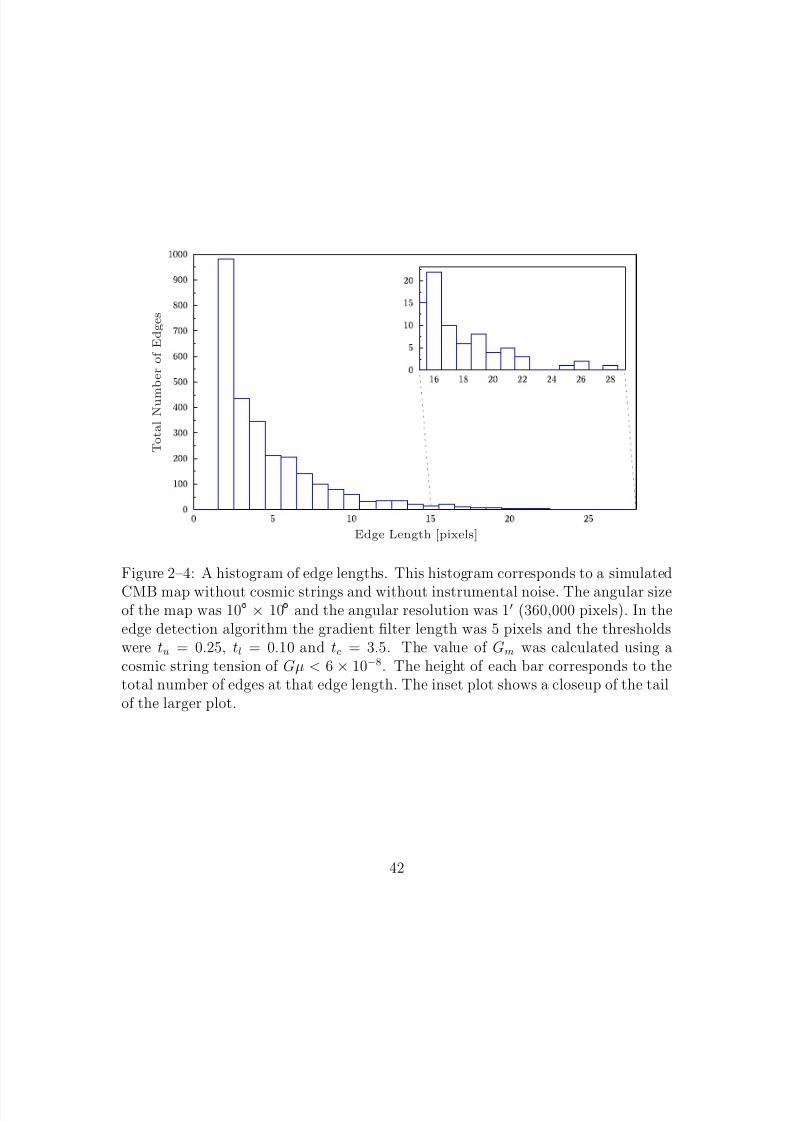
8/3/2019 Andrew Stewart- Constraining cosmological parameters with the cosmic microwave background
http://slidepdf.com/reader/full/andrew-stewart-constraining-cosmological-parameters-with-the-cosmic-microwave 51/93
T o t a l N u m
b e r o f E d g e s
Edge Length [pixels]
Figure 2–4: A histogram of edge lengths. This histogram corresponds to a simulated
CMB map without cosmic strings and without instrumental noise. The angular sizeof the map was 10 × 10 and the angular resolution was 1′ (360,000 pixels). In theedge detection algorithm the gradient filter length was 5 pixels and the thresholdswere tu = 0.25, tl = 0.10 and tc = 3.5. The value of Gm was calculated using acosmic string tension of Gµ < 6 × 10⁻⁸. The height of each bar corresponds to thetotal number of edges at that edge length. The inset plot shows a closeup of the tailof the larger plot.
42
8/3/2019 Andrew Stewart- Constraining cosmological parameters with the cosmic microwave background
http://slidepdf.com/reader/full/andrew-stewart-constraining-cosmological-parameters-with-the-cosmic-microwave 52/93
2.5 Statistical Analysis
Now that we have a numerical description of our edge maps we need to develop
a way to compare them and look for differences. Specifically, we are looking for
a change in the distribution of the total number of edges between an edge map
corresponding to a simulation without cosmic strings and an edge map corresponding
to a simulation with cosmic strings.
Both the Gaussian and string components in the simulated CMB temperature
anisotropy maps are generated using random processes. If we were to compare two
histograms generated from only one simulated temperature anisotropy map each, we
would not be able to draw a very meaningful conclusion. Therefore, to make our
comparison more robust, we simulate many temperature anisotropy maps with the
same input parameters and perform the edge detection and length counting on each
one separately. This provides a set of histograms from which we can then compute
the mean number of edges of each length occurring over all the runs. We also compute
the standard deviation from each mean value. In the end this provides us with a
new averaged histogram of edge lengths that has statistical error bars. Comparing
two of these averaged histograms then allows us to assign a statistical significance to
the difference in the distributions. Figure 2–5 shows a typical averaged histogram.
The distribution of edges is very similar to that for a single simulated map, as shown
in Figure 2–4. The statistical error bars computed over all of the maps are small
compared to the mean value for short lengths. However, they become of the order
of the mean for longer lengths, since those edges are rare. From this point on,
43

8/3/2019 Andrew Stewart- Constraining cosmological parameters with the cosmic microwave background
http://slidepdf.com/reader/full/andrew-stewart-constraining-cosmological-parameters-with-the-cosmic-microwave 53/93
whenever we mention a histogram we mean an averaged histogram computed using
many simulations.
When comparing two histograms, we compare the mean value for each specific
length separately, rather than perform a single general test based on the overall
shapes of the distributions. We prefer to treat each bin separately because each has
a separate standard deviation associated with it. Furthermore, we assume that the
underlying values used to compute each mean are normally distributed. That way
we can use Student’s t-statistic to determine the significance of the difference at each
length.
For two samples of equal size n, Student’s t-statistic is defined as
t =
N 1 − N 2 n
(σ1)2 + (σ2)2, (2.27)
where N 1 and σ1 are the mean and sample standard deviation of the first sample
and N 2 and σ2 are the mean and sample standard deviation of the second sample.
Given two histograms, we compute t for each length occurring in the two histograms
for which N i ≥ 3σi, where i = 1, 2. This constraint on the lengths we consider stems
from our assumption that the underlying distribution of each mean value is normal.
Since it would be inconsistent to consider negative values for the total number of
strings at any given length, we choose only lengths for which the total number of
strings is positive definite at the 3σ level. The p-value corresponding to each t is
then computed from a t-distribution with 2n − 2 degrees of freedom.
44

8/3/2019 Andrew Stewart- Constraining cosmological parameters with the cosmic microwave background
http://slidepdf.com/reader/full/andrew-stewart-constraining-cosmological-parameters-with-the-cosmic-microwave 54/93
M e a n N
u m b e r o f E d g e s
Edge Length [pixels]
Figure 2–5: An averaged histogram of edge lengths. This averaged histogram corre-sponds to 40 simulated CMB maps without cosmic strings and without instrumental
noise. The angular size of each map was 10 × 10 and the angular resolution of each was 1′ per pixel (360,000 pixels). In the edge detection algorithm the gradientfilter length was 5 pixels and the thresholds were tu = 0.25, tl = 0.10 and tc = 3.5.The value of Gm was calculated using a cosmic string tension of Gµ < 6 × 10⁻⁸. Theheight of each bar corresponds to the mean number of edges at that edge length. Theerror bars represent a spread of 3σ from the mean value, where σ is the standarddeviation of the mean, which is calculated separately for each length. Shown hereare only the lengths in the histogram for which the mean is greater than 3σ.
45

8/3/2019 Andrew Stewart- Constraining cosmological parameters with the cosmic microwave background
http://slidepdf.com/reader/full/andrew-stewart-constraining-cosmological-parameters-with-the-cosmic-microwave 55/93
We then combine the probabilities calculated for each length, denoted by pL,
into a single statistic which characterizes the difference between the two histograms.
Using Fisher’s combined probability test, we can define the new statistic χ2
as
χ2 = −2LmL=2
ln( pL) , (2.28)
where Lm is the maximum length at which a p-value was computed. The final p-value
corresponding to the statistic χ2 is then determined from a chi-square distribution
with 2Lm − 2 degrees of freedom.
The final step is to compare this single p-value to a significance level ǫ to conclude
whether or not the difference in the two histograms is significant. We choose to work
with the customary significance level ǫ = 0.0027 corresponding to 3σ of a normal
distribution. If our p-value is less than ǫ we state that the difference in the two edge
maps is statistically significant.
2.6 Results
We present the results of running the Canny edge detection algorithm on simu-
lated CMB anisotropy maps in two parts. First, we report the results for simulations
which are designed to mimic the expected output from the SPT. Using these re-
sults, we determine what kind of bound on the cosmic string tension one could hope
to achieve using the edge detection method on data from that survey. Second, we
present the results for simulations corresponding to a hypothetical survey that has
different specifications than those of the SPT. We use these results to investigate
46

8/3/2019 Andrew Stewart- Constraining cosmological parameters with the cosmic microwave background
http://slidepdf.com/reader/full/andrew-stewart-constraining-cosmological-parameters-with-the-cosmic-microwave 56/93
how the potential constraint on the tension changes with respect to the design of the
survey.
The SPT is capable of producing a 4,000 square degree survey of the anisotropies
in the CMB [37]. To replicate the same amount of sky coverage, we simulate 40 sep-
arate 10 × 10 maps, where the angular resolution of each of these maps is 1 ′ per
pixel, again matching that specified for the SPT. To test the edge detection method,
we simulate two separate sets of 40 maps, the first set including the effect of cosmic
strings, and the second set excluding the effect of cosmic strings. Each set of maps
gives rise to a histogram of edge lengths via the edge detection and edge lengthcounting algorithms. We then compare these two histograms using the statistical
analysis described in Section 2.5 to determine if the difference in the distributions
is significant. We repeat this process for many different values of the cosmic string
tension, until we can no longer identify a statistically significant difference in the two
histograms. Figure 2–6 shows a side by side comparison of a simulated CMB map
without a cosmic string component and a simulated CMB map which does include
a cosmic string component. The effect of the cosmic strings in the final temperature
anisotropy map is not apparent and any difference in the typical structure between
the two maps is unnoticeable by eye. Figure 2–7, on the other hand, shows a his-
togram corresponding to a set of maps without a cosmic string component and a
histogram corresponding to a set of maps with a cosmic string component. The two
histograms show that the edge detection method is in fact able to detect a difference
which is not evident by eye, with maps including strings having slightly higher mean
47
8/3/2019 Andrew Stewart- Constraining cosmological parameters with the cosmic microwave background
http://slidepdf.com/reader/full/andrew-stewart-constraining-cosmological-parameters-with-the-cosmic-microwave 57/93
values for certain lengths. Although the difference in histograms may not seem large,
this particular example would generate a significant result.
Although the angular size and resolution of the simulation are determined by
the specifications of the survey in question, the values of the other free parameters
in each step of process must also be fixed. We take the number of cosmic strings
per Hubble volume in all of the string component simulations to be M = 10 [33],
regardless of the cosmic string tension. In every run of the edge detection algorithm,
we choose the gradient filter length to be 5 pixels, the value of the upper threshold
to be tu = 0.25 and the value of the lower threshold to be tl = 0.10. These values forthe thresholds may appear small, but as one can see from the scale in Figure 2–3,
the gradient magnitude in the string component can take a large range of values.
Therefore, Gm can be quite a bit larger than the average gradient magnitude on a
string induced edge, so we must choose low values for the thresholds in order to not
throw away the entire string signal. We have not mentioned the value of the scaling
factor in the map addition, α, nor the value of the cutoff threshold, tc. The reason is,
we do not fix the value of these two parameters for all of the runs. In the case of the
scaling factor, its value must change for each given cosmic string tension, as described
by Equation (2.7). The value of the cutoff threshold, on the other hand, is chosen
deliberately based on the value of the tension, such that we get the best results from
our edge detection method. We note the value of both of these parameters when
presenting our findings.
For the SPT specific simulations, the capability of the edge detection method
to make a significant detection of the cosmic string signal for different choices of the
48

8/3/2019 Andrew Stewart- Constraining cosmological parameters with the cosmic microwave background
http://slidepdf.com/reader/full/andrew-stewart-constraining-cosmological-parameters-with-the-cosmic-microwave 58/93
3.55e-5 -3.82e-5 2.76e-5 -2.53e-5
Figure 2–6: Comparison of CMB maps with and without a component of cosmic
string induced fluctuations. On the left is the map without a cosmic string componentand on the right is the map with a cosmic string component. Both maps show a 2.5
× 2.5 patch of sky at 1′ resolution (22,500 pixels). The values of the free parametersin the cosmic string simulation were Gµ = 6 × 10⁻⁸ and M = 10. The scaling factorin the map component addition that produced the map on the right was α = 0.987.
49

8/3/2019 Andrew Stewart- Constraining cosmological parameters with the cosmic microwave background
http://slidepdf.com/reader/full/andrew-stewart-constraining-cosmological-parameters-with-the-cosmic-microwave 59/93
M e a n N u m b e r o f E d g e s
Edge Length [pixels]
Without cosmic stringsWith cosmic strings
Figure 2–7: Comparison of histograms for maps with and without a componentof cosmic string induced fluctuations. Each histogram corresponds to a set of 40simulated CMB maps. The angular size of each map was 10
×10 and the angular
resolution of each was 1′ per pixel (360,000 pixels). In the maps including a cosmicstring component, the string free parameters were taken to be Gµ < 6 × 10⁻⁸ andM = 10 while the scaling factor in the map component addition was α = 0.987. Inthe edge detection algorithm the gradient filter length was 5 pixels and the thresholdswere tu = 0.25, tl = 0.10 and tc = 3.5. The value of Gm was calculated using thesame cosmic string tension given above. The height of each bar corresponds to themean number of edges at that edge length. The error bars represent a spread of 3σfrom the mean value, where σ is the standard deviation of the mean. Shown hereare only the lengths for which the mean is greater than 3σ in both histograms.
50

8/3/2019 Andrew Stewart- Constraining cosmological parameters with the cosmic microwave background
http://slidepdf.com/reader/full/andrew-stewart-constraining-cosmological-parameters-with-the-cosmic-microwave 60/93
Table 2–2: Summary of the ability of the Canny algorithm to make a significantdetection of a cosmic string signal for SPT specific simulations. Shown here arethe results corresponding to simulated CMB maps excluding instrumental noise aswell as simulated CMB maps including instrumental noise. In the first column are
different choices for the tension of the cosmic strings. In the second, third and fourthcolumns are the values of the scaling factor, cutoff threshold and p-value respectively,corresponding to each of the tensions. A p-value of less than 2.7 × 10⁻³ indicatesthat the simulations including cosmic strings produced significantly different resultsfrom those without cosmic strings.
String Tension (Gµ) Scaling Factor (α) Cutoff Threshold (tc) p-valueWithout Instrumental Noise
6.0 × 10⁻⁸ 0.987 3.5 7.19 × 10⁻¹²
5.5 × 10⁻⁸ 0.989 4.2 6.99 × 10⁻⁴
5.0 × 10
−8
0.991 5.5 2.39 × 10
−3
4.5 × 10⁻⁸ 0.993 6.0 9.95 × 10⁻³
With Instrumental Noise6.0 × 10−8 0.987 3.5 2.92 × 10⁻¹⁰
5.5 × 10⁻⁸ 0.989 4.2 1.45 × 10⁻³
5.0 × 10⁻⁸ 0.991 5.5 1.36 × 10⁻²
4.5 × 10⁻⁸ 0.993 6.0 1.96 × 10⁻²
cosmic string tension is summarized in Table 2–2. We find that our edge detection
method can distinguish a signal arising from cosmic strings down to a tension of
Gµ = 5 × 10⁻⁸. Therefore, if the edge detection method was used on ideal data
from the SPT, but was unable to distinguish a difference from a theoretical data set
without the effect cosmic strings, we could then impose a constraint on the cosmic
string tension of Gµ < 5 × 10⁻⁸.
The above mentioned results were determined from simulated maps which did
not contain a component of instrumental noise. To examine the effect that detector
noise will have on the ability of the edge detection method to constrain the cosmic
string tension, we repeat the same process described above, with the same choices
51

8/3/2019 Andrew Stewart- Constraining cosmological parameters with the cosmic microwave background
http://slidepdf.com/reader/full/andrew-stewart-constraining-cosmological-parameters-with-the-cosmic-microwave 61/93
for all of the parameters, but this time with instrumental noise included in the sim-
ulation of the CMB maps. As mentioned earlier, we simulate a component of white
noise with a given maximum temperature change. Here, we choose the maximum
temperature change caused by the instrumental noise to be δT N,max = 10µK, roughly
corresponding to that planned for the SPT [37]. Figure 2–8 shows a side by side com-
parison of a simulated CMB map which includes instrumental noise and one which
does not. The effect that the noise has on the map is clear, making it appear pix-
elated and non-Gaussian, yet the overall structure of the image is still visible since
the temperature fluctuations caused by the noise are sub-dominant compared to the
Gaussian fluctuations.
For the SPT specific simulations including instrumental noise, the results of
using the edge detection method to detect a cosmic string signal are also presented
in table 2–2. We find that detector noise does not have a substantial effect, and it
weakens the possible constraint that the edge detection method could place on the
cosmic string tension only slightly to Gµ < 5.5
×10−8.
Along with the results specific to the SPT, we explore how the constraint which
could be applied by the edge detection method changes based on the specifications
of the survey. For this purpose, we imagine a theoretical observatory which has the
same specifications as the SPT but could map five times the amount of sky with the
same resolution, that is, produce a 20,000 square degree survey of the anisotropies in
the CMB. To replicate the output of a survey with this design, we instead simulate
200 separate 10 × 10 maps at 1′ resolution. In this hypothetical case we again
choose the maximum temperature change caused by the instrumental noise to be
52

8/3/2019 Andrew Stewart- Constraining cosmological parameters with the cosmic microwave background
http://slidepdf.com/reader/full/andrew-stewart-constraining-cosmological-parameters-with-the-cosmic-microwave 62/93
3.55e-5 -3.82e-5 3.91e-5 -3.64e-5
Figure 2–8: Comparison of CMB maps with and without a component of instrumen-tal noise. On the left is a simulated CMB map excluding instrumental noise. Onthe right is a simulated CMB map including a component of instrumental noise withmaximum temperature fluctuation δT N,max = 10 µK. Both maps show a 2.5 × 2.5
patch of sky at 1′ resolution (22,500 pixels). Neither map includes a component of cosmic string induced temperature fluctuations.
53
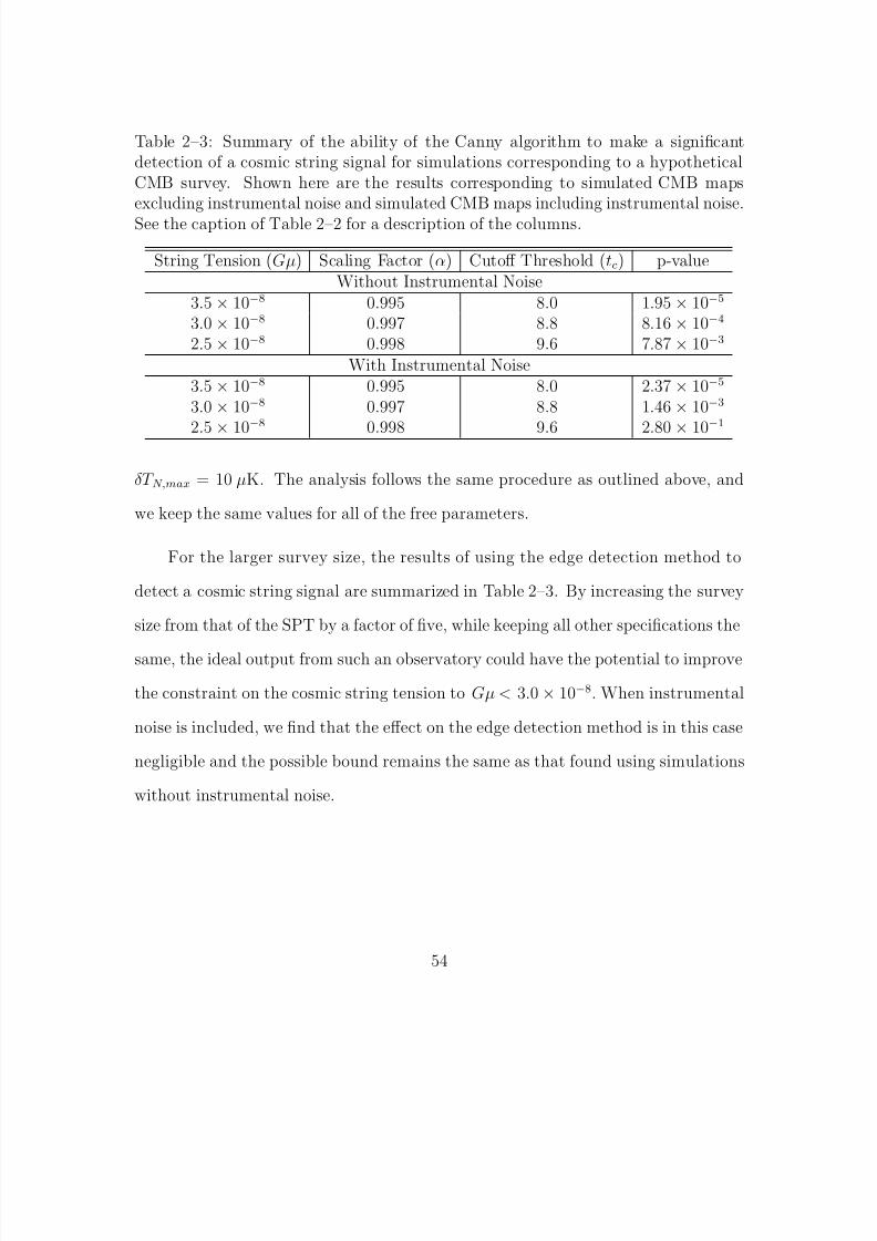
8/3/2019 Andrew Stewart- Constraining cosmological parameters with the cosmic microwave background
http://slidepdf.com/reader/full/andrew-stewart-constraining-cosmological-parameters-with-the-cosmic-microwave 63/93
Table 2–3: Summary of the ability of the Canny algorithm to make a significantdetection of a cosmic string signal for simulations corresponding to a hypotheticalCMB survey. Shown here are the results corresponding to simulated CMB mapsexcluding instrumental noise and simulated CMB maps including instrumental noise.
See the caption of Table 2–2 for a description of the columns.
String Tension (Gµ) Scaling Factor (α) Cutoff Threshold (tc) p-valueWithout Instrumental Noise
3.5 × 10⁻⁸ 0.995 8.0 1.95 × 10⁻⁵
3.0 × 10⁻⁸ 0.997 8.8 8.16 × 10⁻⁴
2.5 × 10⁻⁸ 0.998 9.6 7.87 × 10⁻³
With Instrumental Noise3.5 × 10−8 0.995 8.0 2.37 × 10⁻⁵
3.0 × 10⁻⁸ 0.997 8.8 1.46 × 10⁻³
2.5 × 10⁻⁸
0.998 9.6 2.80 × 10⁻¹
δT N,max = 10 µK. The analysis follows the same procedure as outlined above, and
we keep the same values for all of the free parameters.
For the larger survey size, the results of using the edge detection method to
detect a cosmic string signal are summarized in Table 2–3. By increasing the survey
size from that of the SPT by a factor of five, while keeping all other specifications the
same, the ideal output from such an observatory could have the potential to improve
the constraint on the cosmic string tension to Gµ < 3.0 × 10⁻⁸. When instrumental
noise is included, we find that the effect on the edge detection method is in this case
negligible and the possible bound remains the same as that found using simulations
without instrumental noise.
54

8/3/2019 Andrew Stewart- Constraining cosmological parameters with the cosmic microwave background
http://slidepdf.com/reader/full/andrew-stewart-constraining-cosmological-parameters-with-the-cosmic-microwave 64/93
2.7 Discussion
There is renewed interest in cosmic strings formed during phase transitions in
the early universe despite the fact that they were ruled out as being the single source
of structure formation. The evolution of the random network of cosmic strings over
time has been well studied and accurately modelled. The observational signatures
arising from this cosmic string network lie within observational reach, and many
works have been devoted to finding a string signal in order to constrain the value of
the cosmic string tension, Gµ. The existence of cosmic strings has yet to be verified
or ruled out by observations and the continued search for strings is motivated by
cosmological models in which their formation is generally predicted.
We have developed a method of searching for linear discontinuities in the mi-
crowave background temperature caused by the presence of cosmic strings along our
line of sight to the surface of last scattering. The method which we have developed
involves applying an edge detection algorithm to CMB temperature anisotropy maps
in order to identify the effect of cosmic strings. We have applied our edge detection
method to simulated CMB maps both including cosmic strings, and without cosmic
strings, to test its ability to discriminate between the two. This then translates di-
rectly into a possible constraint on the cosmic string tension. In particular, we have
focused on two different sets of simulations, one which mimics the future output com-
ing from the SPT and one which corresponds to a theoretical survey which covers five
times as much sky as the SPT with the same angular resolution. We find that the
edge detection method could potentially place a bound on the cosmic string tension
55
8/3/2019 Andrew Stewart- Constraining cosmological parameters with the cosmic microwave background
http://slidepdf.com/reader/full/andrew-stewart-constraining-cosmological-parameters-with-the-cosmic-microwave 65/93
of Gµ < 5 × 10⁻⁸ for a perfect CMB observation from the SPT and that this could
be lowered to Gµ < 3 × 10⁻⁸ for the larger survey. For more realistic simulations
which include instrumental noise, we find that the potential bound corresponding
to the SPT weakens by only a small amount to Gµ < 5.5 × 10⁻⁸ while the possible
bound corresponding to the theoretical survey does not change at all, and is still
Gµ < 3 × 10⁻⁸. We consider the constraint corresponding to the SPT specific simu-
lations which include a component of instrumental noise to be the main conclusion of
this work. This possible bound is approximately an order of magnitude better than
those arising from other methods which use CMB observations and approximately
two orders of magnitude better than those arising from other methods which search
for the KS-effect. Therefore, we believe that using the output from the SPT along
with the edge detection method has the potential to greatly improve the constraint
on the cosmic string tension. This bound is not tighter than the constraints arising
from current pulsar timing data, although it is competitive, falling directly within
the range of values reported by different observations. Nevertheless, as mentioned
in the Overview, we consider our method of constraining the tension to be more ro-
bust since we make less assumptions about some of the unknown parameters which
describe the cosmic string network and its evolution. Therefore, we believe that the
possible bound on Gµ given above would in fact represent a stronger constraint.
We conclude that instrumental noise does not have a very major effect on the
ability of the edge detection method to identify the cosmic string signal. We believe
that this is an indication that the thresholding with hysteresis performs as it should,
since noisy pixels could destroy the edge signal by causing large fluctuations in the
56

8/3/2019 Andrew Stewart- Constraining cosmological parameters with the cosmic microwave background
http://slidepdf.com/reader/full/andrew-stewart-constraining-cosmological-parameters-with-the-cosmic-microwave 66/93
gradient magnitude. Furthermore, as one can see from Figure 2–7, the largest dif-
ference between histograms occurs at short lengths rather than longer lengths. The
instrumental noise leaves this difference in the short edge signal between maps with
and without strings relatively unchanged, since the probability of a particularly noisy
pixel falling on a short edge, resulting in it being incorrectly detected by the Canny
algorithm, is small compared to that for longer edges. We also found that increasing
the simulated survey size increases the statistical significance of the deviations be-
tween the histograms for similar values of the cosmic string tension. This behaviour
is expected though, since more edge maps were used to compute the mean values
in each of the histograms and one can see from Equation (2.27) that the value of t
scales as√
n. While the p-values are smaller for similar tensions, the final constraint
which can be levied by the larger survey is not drastically different from that corre-
sponding to the SPT specific simulations. Increasing the survey size by 5 times only
lowered the possible constraint by a factor of roughly√
5. Based on this result, we
conclude that the survey size does not have a major influence on the ability of the
edge detection method.
While we have chosen to focus on the SPT in this work, the edge detection
method is quite versatile and could be used with virtually any high resolution CMB
survey. We conclude that this method presents a powerful and unique way of con-
straining the cosmic string tension which has the potential to perform better than
current methods, or, at the very least, to provide a complimentary technique to those
already in use. In the following, we note some improvements which could be made
to the method and also the way in which it is tested.
57

8/3/2019 Andrew Stewart- Constraining cosmological parameters with the cosmic microwave background
http://slidepdf.com/reader/full/andrew-stewart-constraining-cosmological-parameters-with-the-cosmic-microwave 67/93
When generating the simulated CMB maps, we employed a toy model of the
cosmic string network which includes only straight strings and no cosmic string
loops. More detailed models of the network and its evolution have been developed
in other works [18, 19, 20, 40] and can be implemented numerically. Therefore,
one obvious way to improve the testing method we have outlined here would be to
implement one of these more complex models which would in turn produce a more
realistic map of the temperature anisotropies induced via the KS-effect. On the other
hand, we stress that a change of this nature would come at a large computational
expense. On a similar note, it may also be useful to develop a more robust method
of combining the string induced temperature anisotropies with those coming from
Gaussian fluctuations, to make sure that the final simulated map agrees with other
observations.
While on the topic of the simulated CMB maps, we reiterate that we have
included only a simplified white noise component as instrumental noise. A more
complex simulation of instrumental noise would include a low frequency piece which
results in stripes appearing in the final map of the CMB. Based on the method
described in this thesis, it is clear that this striping would be crucial, since it would
result in maps with more edges than that predicted by the cosmological theory and
this could be confused with the effect of cosmic strings. One redeeming feature of this
type of low frequency noise is that the stripes which are introduced would lie along
the scanning direction, thus, when dealing with actual SPT data, it may be possible
to subtract this effect out of the final map or to simply ignore edges lying along the
known scanning direction in the edge detection algorithm itself. In future work it
58

8/3/2019 Andrew Stewart- Constraining cosmological parameters with the cosmic microwave background
http://slidepdf.com/reader/full/andrew-stewart-constraining-cosmological-parameters-with-the-cosmic-microwave 68/93
would be useful to investigate this type of noise as well as the removal strategies in
more detail to determine if they would change the behavior of the edge detection
method and whether they could weaken the limits quoted here.
Lastly, after applying the Canny edge detection algorithm to the CMB temper-
ature anisotropy maps, we quantify the corresponding edge map by recording the
length of every edge appearing in it. As mentioned in Section 2.4, this is one of the
simplest ways of describing the edge map, and it may be beneficial to investigate
an alternative method of image comparison which provides a more powerful way of
discriminating between the two edge maps.
59
8/3/2019 Andrew Stewart- Constraining cosmological parameters with the cosmic microwave background
http://slidepdf.com/reader/full/andrew-stewart-constraining-cosmological-parameters-with-the-cosmic-microwave 69/93
CHAPTER 3
Constraint on the Blue Tilt of Tensor Modes1
3.1 Overview
A stochastic background of primordial gravitational waves represents valuable
information about the very early universe as well as a way to discriminate between
the myriad of cosmological models currently proposed. Although a stochastic back-
ground of gravitational waves has yet to be directly detected, efforts are being un-
dertaken to do so by many current and future experiments, some of the largest being
LIGO, GEO600, TAMA, and LISA [44]. As mentioned in the introduction, CMB
polarization also offers a way to detect a signature generated by inflationary grav-
itational waves. The CMB polarization observations could provide one of the two
detections needed in order to determine the slope of the gravitational wave spectrum.
1 The results of this portion of the thesis led to the publication [43]. The work was co-authored
by R. H. Brandenberger who made some slight revisions to the final text.
60

8/3/2019 Andrew Stewart- Constraining cosmological parameters with the cosmic microwave background
http://slidepdf.com/reader/full/andrew-stewart-constraining-cosmological-parameters-with-the-cosmic-microwave 70/93
Furthermore, they allow the value of the tensor to scalar ratio to be determined at
large scales.
A stochastic background of gravitational waves is characterized by the gravita-
tional wave spectrum
Ωgw =1
ρc
dρgwd ln f
, (3.1)
where ρc is the critical density of the universe, ρgw is the energy density of the
background gravitational waves and f is frequency [44]. In the above, the energy
density in gravitational waves is written as an integral over ln f , and the derivative
picks out the integrand. In practise, the gravitational wave spectrum is commonly
assumed to depend on frequency as a power of f . The value of this power is denoted
by nT , and is known as the tensor spectral index.
Within the framework of the inflationary universe scenario the primordial grav-
itational wave spectrum is predicted to be nearly scale invariant with a slight red tilt
[45], i.e. more power at large scales. The reason for the red tilt is that the amplitude
of the gravitational wave spectrum on a fixed scale k is set by the Hubble constant
H at the time ti(k) when the scale k exits the Hubble radius during the period of
inflation. Smaller scales exit the Hubble radius later when the Hubble constant is
smaller, leading to the red tilt. However, there do exist alternative cosmological
models to the standard inflationary scenario which predict a blue tilt of the gravita-
tional wave spectrum, i.e. more power at small scales, which have not yet been ruled
out by observations. One cosmological model that predicts such a tilt is string gas
cosmology [46].
61

8/3/2019 Andrew Stewart- Constraining cosmological parameters with the cosmic microwave background
http://slidepdf.com/reader/full/andrew-stewart-constraining-cosmological-parameters-with-the-cosmic-microwave 71/93
String gas cosmology is an approach to string cosmology which starts from the
new degrees of freedom and symmetries which string theory contains, but particle
physics-based models lack, namely string winding modes, string oscillatory modes
and T-duality symmetry, and uses them to develop a new cosmological model [46].
The claim is that by making these crucial stringy additions, one obtains a new
cosmological model which is singularity free [46], generates nearly scale-invariant
scalar metric perturbations from initial string thermodynamic fluctuations [47, 48]
and provides a natural explanation for the observed dimensionality of space [46] (see
[49] for an overview of the string gas cosmology structure formation scenario). A
key result which emerges from string gas cosmology is that the gravitational wave
spectrum has a slight blue tilt, giving rise to a testable prediction different from that
of the inflationary universe paradigm [50].
The goal of the second part of this work is to investigate how a tensor spectrum
with a blue tilt can be constrained by the measurements of the CMB, and how this
compares to similar constraints derived from other astrophysical observations. The
motivation for this is provided by string gas cosmology, yet these constraints apply to
all cosmological models. We believe that precise numerical constraints on the tensor
spectral index have not been presented in the literature and this analysis represents
an important result.
The remainder of this chapter is arranged as follows: In Section 3.2, we use
pulsar timing, laser interferometer and big bang nucleosynthesis constraints on the
gravitational wave spectrum to calculate the bounds on the required blue tilt. We
also investigate the prospects for improved constraints from some future experiments.
62

8/3/2019 Andrew Stewart- Constraining cosmological parameters with the cosmic microwave background
http://slidepdf.com/reader/full/andrew-stewart-constraining-cosmological-parameters-with-the-cosmic-microwave 72/93
In Section 3.3, we present the results of our analysis into whether the angular power
spectrum of the CMB temperature anisotropy is compatible with the bounds calcu-
lated from the other observations, or if it will offer an even tighter constraint. Lastly,
in Section 3.4, we discuss our findings and other issues related to the method used.
3.2 Current Bounds from Other Observations
The starting point of our analysis will be an expression for the primordial grav-
itational wave spectrum normalized by CMB observations. Chongchitnan and Efs-
tathiou [51] have derived just such an expression with a pivot scale k0 = 0.002Mpc−1
using the combined results from multiple surveys. Using a value P S (k0) ≃ 2.21×10⁻⁹
for the amplitude of the scalar power spectrum evaluated at the pivot scale, they
found Ωgw(f ) can be written as
h2Ωgw(f ) ≃ 4.36 × 10⁻¹⁵r
f
f 0
nT
, (3.2)
where f 0 = 3.10 × 10⁻¹⁸
Hz. Solving this result for the tilt of the gravitational wave
spectrum we get the explicit expression
nT ≃ 1
ln(f ) − ln(f 0)ln
2.29 × 10¹⁴
h2Ωgw(f )
r
. (3.3)
In the above equations r is the tensor-to-scalar ratio evaluated at the pivot scale,
r =P T (k0)
P S (k0)
. (3.4)
63

8/3/2019 Andrew Stewart- Constraining cosmological parameters with the cosmic microwave background
http://slidepdf.com/reader/full/andrew-stewart-constraining-cosmological-parameters-with-the-cosmic-microwave 73/93
The calculation of the tensor-to-scalar ratio depends quite sensitively on the pa-
rameters of the cosmological model under consideration. For that reason we choose
to leave r as a free parameter in the main expressions calculated in this work. Nev-
ertheless, for the sake of examining some numerical values of the constraints derived
here, we will insert a value of r corresponding to the current upper bound into our
results. Note, however, that the bounds we derive depend only logarithmically on
r. In each case we choose to use the value of the tensor-to-scalar ratio given by
the combined three-year WMAP and lensing normalized Sloan Digital Sky Survey
(SDSS) data2 applied to the standard ΛCDM model, but including tensors [45].
3.2.1 Pulsar Timing
High precision measurements of millisecond pulsars provide a natural way to
study low frequency gravitational waves. A gravitational wave passing between the
earth and a pulsar will cause a slight change in the time of arrival of the pulse
leading to a detectable signal. In the case of gravitational waves, the fluctuating
time of arrivals will be correlated between widely spaced pulsars, producing a unique
signature. Therefore, it can be discriminated from other effects which can cause a
varying time of arrival for a single pulsar. Jenet et al. [53] have developed a technique
to make a definitive detection of a stochastic gravitational wave background which
involves cross-correlating the time derivative of the timing residuals for multiple
2 We note that this portion of the work was completed before the release of the five-year WMAPresults [7], but this new data would not have a significant effect on any part of this study.
64

8/3/2019 Andrew Stewart- Constraining cosmological parameters with the cosmic microwave background
http://slidepdf.com/reader/full/andrew-stewart-constraining-cosmological-parameters-with-the-cosmic-microwave 74/93
pulsars. The value of Ωgw is then determined directly from the power spectrum of
the timing residuals [53]. The significance of a detection using the method of Jenet
et al. depends on the number of pulsars observed, the rms timing noise, the number
of observations and the power spectrum of the measured timing residuals.
The Parkes Pulsar Timing Array (PPTA) project [52] is a pulsar timing exper-
iment using the Parkes 64m radio telescope located in Australia with the ultimate
goal of reaching the required sensitivity to make a direct detection of gravitational
waves. The PPTA project hopes to make timing observations of a sample of twenty
millisecond pulsars, ten or more of which with a precision of less than approximately100 ns.
Jenet et al. have applied their method to data from seven pulsars observed
by the PPTA project combined with an earlier data set to find a constraint on the
amplitude of the characteristic strain spectrum. They then used this result to place
a bound on the primordial gravitational wave spectrum [28]
h2Ωgw(1/8 yr) ≤ 2.0 × 10⁻⁸ . (3.5)
Plugging this bound into Equation (3.3) at the frequency f = 1/8yr ≃ 3.96×10⁻⁹Hz,
we obtain a constraint on the tensor spectral index
nT 0.0477ln
4.59 × 10⁶
r
. (3.6)
The WMAP+SDSS data places a bound r < 0.30 on the tensor-to-scalar ratio [45].
Inserting r = 0.30 into the above equation we find that the current pulsar timing
observations constrain the blue tilt of the tensor spectrum to nT 0.79.
65

8/3/2019 Andrew Stewart- Constraining cosmological parameters with the cosmic microwave background
http://slidepdf.com/reader/full/andrew-stewart-constraining-cosmological-parameters-with-the-cosmic-microwave 75/93
Jenet et al. have also used simulated data to determine the upper bound on the
primordial gravitational wave spectrum expected from future pulsar observations.
Using a simulated data-set of twenty pulsars timed with an RMS timing residual of
100 ns over 5 years they calculated [28]
h2Ωgw(1/8 yr) ≤ 9.1 × 10⁻¹¹ . (3.7)
Plugging this improved constraint into Equation (3.3) at the frequency f = 1/8 yr
we calculate a bound
nT 0.0477ln2.09 × 104
r , (3.8)
and again using the value r = 0.30, we find that, in the absence of a detection, future
pulsar timing observations could tighten the constraint on the blue tilt to nT 0.53.
3.2.2 Interferometers
Interferometer experiments offer a way to directly measure the gravitational
wave strain spectrum with many observatories currently running or planned for the
future. Interferometers in different locations form a network that will search for a
correlated signal between detectors beneath uncorrelated detector noise, in order to
improve sensitivity.
The Laser Interferometer Gravitational Wave Observatory (LIGO) [54] is a
ground based interferometer project operating in the frequency range of 10 Hz -
a few kHz. LIGO consists of two collocated Michelson interferometers in Hanford,
66

8/3/2019 Andrew Stewart- Constraining cosmological parameters with the cosmic microwave background
http://slidepdf.com/reader/full/andrew-stewart-constraining-cosmological-parameters-with-the-cosmic-microwave 76/93
Washington, H1 with 4 km long arms, and H2 with 2 km long arms, along with a
third interferometer in Livingston Parish, Louisiana, L1 with 4 km long arms.
Most recently LIGO has performed its fourth science run, S4, with improved
interferometer sensitivity. Abbott et al. [54] have used the S4 data to calculate
a limit on the amplitude of a frequency independent gravitational wave spectrum.
They computed a bound
Ωgw < 6.5 × 10⁻⁵ (3.9)
in the frequency range 51-150 Hz. Inserting this value into Equation (3.3) at the
frequency f = 100 Hz, we get a constraint
nT 0.0223 ln
1.49 × 10¹⁰h2
r
. (3.10)
The WMAP+SDSS data also provides a value of h = 0.716 for the Hubble param-
eter3 . Inserting this along with r = 0.30 into the above bound, we find that the
current LIGO results place a constraint nT 0.53 on the blue tilt of the tensor
spectrum.
The final phase of LIGO, named Advanced LIGO, hopes to reach a detection
sensitivity of [54]
Ωgw ∼ 10−9 . (3.11)
3 The complete parameter table is available on-line at: http://lambda.gsfc.nasa.gov/
product/map/dr2/params/lcdm_tens_wmap_sdss.cfm
67

8/3/2019 Andrew Stewart- Constraining cosmological parameters with the cosmic microwave background
http://slidepdf.com/reader/full/andrew-stewart-constraining-cosmological-parameters-with-the-cosmic-microwave 77/93
Plugging this value into Equation (3.3) at f = 100 Hz, we find that if Advanced
LIGO does not make a positive detection of a gravitational wave background, then
it will place a bound on the blue tilt of the tensor spectrum
nT 0.0223 ln
2.29 × 10⁵h2
r
. (3.12)
Using r = 0.30 and h = 0.716 in this expression, Advanced LIGO would then
constrain the blue tilt of the tensor spectrum to nT 0.29.
The Laser Interferometer Space Antenna (LISA) [55] is a planned space-based
interferometer experiment operating in the mHz range. LISA will consist of threedrag-free spacecraft each at the corner of an equilateral triangle with sides of length
5 × 10⁹ m. Each spacecraft has two optical assemblies pointed towards the other
two spacecraft forming three Michelson interferometers. This triangle formation will
orbit the sun in an Earth-like orbit separated from us by approximately fifty million
kilometres. The goal of LISA is to reach a sensitivity of [56]
h2
Ωgw(1 mHz) ≃ 1 × 10⁻¹²
. (3.13)
At the LISA sensitivity level one would expect gravitational wave signals from super-
massive black hole binaries, other binary systems and super-massive black hole for-
mation to be present. Assuming these predicted signals could somehow be removed
and LISA does not detect any primordial signal, we can plug this predicted bound
into Equation (3.3) at f = 1 mHz to obtain a limit on the blue tilt of the primordial
68

8/3/2019 Andrew Stewart- Constraining cosmological parameters with the cosmic microwave background
http://slidepdf.com/reader/full/andrew-stewart-constraining-cosmological-parameters-with-the-cosmic-microwave 78/93
gravitational wave spectrum
nT 0.0299ln2.29 × 102
r . (3.14)
Inserting r = 0.30 into this equation we find that LISA could potentially place a
constraint nT 0.20 on the blue tilt.
3.2.3 Nucleosynthesis
The theory of big-bang nucleosynthesis (BBN) successfully predicts the observed
abundances of several light elements in the universe. In doing so, BBN places con-
straints on a number of cosmological parameters. This in turn results in an indirect
constraint on the energy density in a gravitational wave background as follows: the
presence of a significant amount of gravitational radiation at the time of nucleosyn-
thesis will change the total energy density of the universe, which affects the rate of
expansion in that era, leading to an over-abundance of helium and thus spoiling the
predictions of BBN [44].
Assuming N ν = 4.4, where N ν is the effective number of neutrino species at the
time of nucleosynthesis, the BBN bound is [54]
f 2f 1
Ωgw(f ) d(ln f ) < 1.5 × 10⁻⁵ . (3.15)
Plugging Equation (3.2) into the left-hand side and performing the integration we
obtain the inequalityf nT 2 − f nT 1
nT < 3.4 × 10⁹
h2f nT 0
r. (3.16)
69

8/3/2019 Andrew Stewart- Constraining cosmological parameters with the cosmic microwave background
http://slidepdf.com/reader/full/andrew-stewart-constraining-cosmological-parameters-with-the-cosmic-microwave 79/93
In order to apply the above result, we must first discuss the two integration limits
f 1 and f 2. The lower cutoff frequency f 1 corresponds to the Hubble radius at the
time of BBN and takes the value f 1 ∼ 10−10
Hz. For wavelengths larger than the
Hubble radius, the gravitational waves are frozen out [57] (see [58] for a review) and
thus do not act like radiation. The upper cutoff frequency f 2 is the ultraviolet cutoff.
We will take it to be given by the Planck frequency, i.e. f 2 = f Pl = 1.86 × 1043 Hz.
Substituting these two limits into Equation (3.16) along with the WMAP+SDSS
values r = 0.30 and h = 0.716 then solving numerically for nT , we find the bound
on the blue tilt of the tensor spectrum from BBN to be
nT 0.15 . (3.17)
Had we instead inserted for f 2 the scale of grand unification, 1016GeV, or the Hubble
rate during a simple large field inflation model, which is 1013 GeV, the bound would
be slightly relaxed to 0.16 or 0.17, respectively. Thus, the dependence of the bound
on the uncertain ultraviolet cutoff scale f 2 is quite mild.
We do not want Ωgw > 1 at any scale within the integration bounds. Since
we are working with such large frequencies we should check to be sure that this
condition is satisfied. Substituting the value of the tensor spectral index determined
by BBN back into Equation (3.2) we find that Ωgw(f Pl) = 3.93 × 10⁻⁶, meaning our
requirement is indeed satisfied for all frequencies within the interval of integration.
70

8/3/2019 Andrew Stewart- Constraining cosmological parameters with the cosmic microwave background
http://slidepdf.com/reader/full/andrew-stewart-constraining-cosmological-parameters-with-the-cosmic-microwave 80/93
3.3 Results
The three-year WMAP results are an improvement upon previous observations.
A reduction in instrument noise produced spectra which are three times more sensi-
tive in the noise limited region, independent years of data allow for cross-checks, the
instrument calibration and response have been better characterized and a thorough
analysis of the polarization data has improved the understanding of the data [59].
Using the three-year WMAP data, the derived angular power spectrum of the tem-
perature anisotropy, C l, is cosmic variance limited to l = 400 and the signal to noise
ratio exceeds unity to l = 1000 [59]. Thus, this high precision cosmological data may
provide another method of constraining the value of the tensor spectral index.
Using camb, we can simulate how a blue tilt of the primordial gravitational
wave background would effect the observed angular power spectrum of the CMB. To
examine possible constraints, we employ the following method: First, we calculate
C l using camb for each of the three current bounds on nT calculated in the previous
sections. Second, we calculate C l using camb, but this time with the standard
inflationary relation nT = −r/8 [45]. Finally, we compare the output C l values for
the models with a blue tilt against the output for the model with the standard value
of the tensor spectral index (i.e. the above relation from inflationary cosmology).
For consistency with the previous sections, when running camb we choose our input
cosmological parameters to be those calculated using the WMAP+SDSS data for a
ΛCDM model with tensors.
71

8/3/2019 Andrew Stewart- Constraining cosmological parameters with the cosmic microwave background
http://slidepdf.com/reader/full/andrew-stewart-constraining-cosmological-parameters-with-the-cosmic-microwave 81/93
10 102
103
0
100
200
300
400
500
600
700
800
900
l
D i ff e r e n c e µ K 2
Figure 3–1: Magnitude of the difference between the angular power spectra of amodel with a blue tensor spectral index and a model with a standard tensor spectralindex. Shown here are the cases nT = 0.15 (green), nT = 0.53 (yellow) and nT = 0.79(orange) respectively. The dashed line represents the cosmic variance error at eachl.
From Figure 3.3 we can clearly see that the power spectrum of the temperature
anisotropy for models with a blue tensor spectral index does not vary much from
that calculated using a standard inflationary definition of the tensor spectral index.
In fact, the difference is within the cosmic variance error at all l ≤ 1000 for each of
the three bounds calculated using the PPTA observations, LIGO observations and
the theory of BBN. Thus, we conclude that the CMB does not offer any tighter
constraints on the blue tilt of the gravitational wave spectrum than those already
calculated.
72

8/3/2019 Andrew Stewart- Constraining cosmological parameters with the cosmic microwave background
http://slidepdf.com/reader/full/andrew-stewart-constraining-cosmological-parameters-with-the-cosmic-microwave 82/93
3.4 Discussion
A stochastic background of primordial gravitational waves is a prediction of
many cosmological models. Assuming that the gravitational wave spectrum depends
as a power on frequency, then this spectrum can be characterized by its tilt and
amplitude. Most models predict the tilt to be nearly scale-invariant but slightly red,
while some models, like string gas cosmology, predict a slight blue tilt. Although a
gravitational wave background has yet to be directly detected, observational results
can already be used to constrain it.
Using the current results from pulsar timing observations, direct detection ob-
servations and the theory of nucleosynthesis, we have placed bounds on the possible
blue tilt of the gravitational wave background. By far the tightest constraint on
the tilt comes from big-bang nucleosynthesis. If we take the tensor to scalar ratio
on CMB scales to be given by the current observational upper bound, and if we
take the ultraviolet cutoff scale in the spectrum of gravitational radiation to be the
Planck scale, then the bound is nT 0.15, tighter than even Advanced LIGO, the
future PPTA, and LISA can hope to achieve. It is not surprising that nucleosynthesis
provides the tightest bounds on a blue tilt of the gravitational wave spectrum since
nucleosynthesis probes physics on scales much smaller than the other experiments we
analyzed, and spectra with blue tilts have more power on the smallest scales. That
is, BBN gives us the largest “lever arm” to probe gravitational waves in conjunction
with CMB observations, a point also made in [60]. From our results we can clearly
73

8/3/2019 Andrew Stewart- Constraining cosmological parameters with the cosmic microwave background
http://slidepdf.com/reader/full/andrew-stewart-constraining-cosmological-parameters-with-the-cosmic-microwave 83/93
see the trend that the bound on the blue tilt of the tensor spectral index tightens as
the length scale probed by the given experiment decreases.
Simulations of the angular power spectrum of the temperature anisotropies in
the CMB did not offer any tighter constraints on the tensor spectral index, with each
of the constraints calculated in this paper producing a temperature power spectrum
that was within the cosmic variance error of one calculated for a standard ΛCDM
model with tensor modes included.
After completion of this work we became aware of [61] in which a master equa-
tion was derived which relates the short wavelength observable Ωgw(f ) to the tensor
to scalar ratio measured with the CMB. The goal of that work was to develop a
formulation which is as general as possible. In particular, the equation of state pa-
rameter and the tensor spectral index are taken to be arbitrary functions of the scale
factor and wavenumber respectively, not constants as is often assumed. Their master
equation is thus a more general version of our “master” equation (3.2) and we could
have just as easily used it as our starting point. In fact, we have confirmed that by
choosing a constant value w = 1/3 for the equation of state parameter (which is de-
scribed as the most logical value in [61]) and numerical values for other cosmological
parameters that match our choices above, we can indeed re-derive all of our results
from the master equation of [61]. We consider this a good consistency check for
the constraints derived in this work. The authors of [61] do include a discussion of
some of the same types of observations mentioned here, namely laser interferometer
and pulsar timing, however, we stress that they do not use the current numerical
constraint from any particular observatories to compute actual upper bounds on nT ,
74
8/3/2019 Andrew Stewart- Constraining cosmological parameters with the cosmic microwave background
http://slidepdf.com/reader/full/andrew-stewart-constraining-cosmological-parameters-with-the-cosmic-microwave 84/93
which was the purpose of this work. The authors of [61] also discuss a constraint
on nT coming from BBN, but they take the constraint on Ωgw from BBN to be a
constant across all frequencies rather than integrating their master equation as was
done in this study. In the end they find a weaker bound on the tilt, nT 0.36, than
the one obtained here.
As mentioned in Section 3.2 , Equation (3.2) has been normalized at the scale
of cosmic microwave background observations. However, those experiments probe
scales that are approximately ten orders of magnitude larger than those probed by
the PPTA and approximately nineteen orders of magnitude larger than those probedby LIGO, with LISA probing between the two. Extrapolating between such a large
difference in scales is not straightforward and we note that in [51] the authors con-
clude from their analysis that even within the framework of the inflationary universe
paradigm the formula for the primordial gravitational wave spectrum (3.2) is too re-
strictive, and they believe it is indeed not possible to extrapolate reliably over such a
large difference in scales. Whether or not this is the case in the string gas cosmology
model should perhaps be examined more carefully in future work.
Continuing with string gas cosmology, we conclude that the current bounds on
the tilt of the gravitational wave spectrum are weak. The predicted magnitude of the
blue tilt of the gravity wave spectrum is thought to be comparable to the magnitude
of the red tilt of the spectrum of scalar metric fluctuations [50]. If the latter is taken
to agree with the current bounds, we predict a blue tilt of less than nT = 0.1 which
will not be easy to detect. There may, on the other hand, be models similar to string
75

8/3/2019 Andrew Stewart- Constraining cosmological parameters with the cosmic microwave background
http://slidepdf.com/reader/full/andrew-stewart-constraining-cosmological-parameters-with-the-cosmic-microwave 85/93
gas cosmology in which the scalar and tensor tilts are not related, and for which
planned experiments could set valuable constraints on the model parameter space.
76

8/3/2019 Andrew Stewart- Constraining cosmological parameters with the cosmic microwave background
http://slidepdf.com/reader/full/andrew-stewart-constraining-cosmological-parameters-with-the-cosmic-microwave 86/93
CHAPTER 4
Conclusions
The cosmic microwave background has had, has, and will continue to have im-
portant implications for cosmology. It represents the premier tool with which to gain
insight into the physics of the early universe, as well as a number of other phenomena.
In this thesis, we have explored the ability of the CMB to constrain two particular
parameters related to alternative cosmological models.
We have developed a method which makes use of the Canny edge detection
algorithm as a means of searching maps of the CMB temperature for the signature
of the KS-effect. Since this effect is caused by the presence of cosmic strings, the edge
detection method represents a way of directly constraining the cosmic string tension.
By testing this method on simulated CMB maps, we found that, using the future
output from the South Pole Telescope project, a bound on the cosmic string tension
of Gµ < 5.5 × 10⁻⁸ could potentially be imposed. This bound is approximately an
order of magnitude lower than the best current constraint imposed by the CMB and
is competitive with those reported by from pulsar timing experiments. Nevertheless,
we believe that the edge detection method provides a more robust result than those
77

8/3/2019 Andrew Stewart- Constraining cosmological parameters with the cosmic microwave background
http://slidepdf.com/reader/full/andrew-stewart-constraining-cosmological-parameters-with-the-cosmic-microwave 87/93
from pulsars, since less assumptions about the nature of the cosmic strings have to
be made. We also found that using the edge detection method with data from a
much larger survey observing with the same angular resolution as the SPT would
not drastically reduce the possible constraint that could be levied, reducing it by
only a factor of a few.
We have also investigated whether the angular power spectrum of the CMB
could provide a stronger constraint on the possible blue tilt of the gravitational
wave background than those imposed by other means, namely, pulsar timing and
laser interferometer observations and the theory of nucleosynthesis. As a first step,we calculated the specific constraint on the blue tilt related to each of these three
observations, which we believe represents in itself an important result. We discovered
that the tightest current bound on the blue tilt of the tensor spectrum comes from
BBN at nT 0.15, tighter than even some future gravitational wave observatories
could hope to achieve. In the end, we found that the CMB could not impose a tighter
bound than any of these three methods.
In closing, we believe that in this thesis we have shown two important results as
well as some unique ways of extracting information from the CMB. Considering the
topics focused on in this work, we have highlighted the influence that the CMB has
on a wide range of cosmological issues. Then again, by the same token, we have also
shown that alternative models are still viable, and cannot be entirely ruled out by the
precise measurements which have already been taken. On that note, looking ahead
to the future of CMB physics, we believe that there are still many more exciting
discoveries to be made.
78

8/3/2019 Andrew Stewart- Constraining cosmological parameters with the cosmic microwave background
http://slidepdf.com/reader/full/andrew-stewart-constraining-cosmological-parameters-with-the-cosmic-microwave 88/93
References
[1] A. A. Penzias and R. W. Wilson. A Measurement of excess antenna temperatureat 4080- Mc/s. Astrophys. J., 142:419–421, 1965.
[2] J. C. Mather et al. Early results from the cosmic background explorer (COBE).COBE-PREPRINT-NO.-90-03.
[3] C. L. Bennett et al. The Microwave Anisotropy Probe (MAP) Mission. Astro-
phys. J., 583:1–23, 2003, arXiv:astro-ph/0301158.
[4] J. C. Mather et al. Measurement of the Cosmic Microwave Background spectrumby the COBE FIRAS instrument. Astrophys. J., 420:439–444, 1994.
[5] G. F. Smoot et al. Structure in the COBE differential microwave radiometerfirst year maps. Astrophys. J., 396:L1–L5, 1992.
[6] C. H. Lineweaver, J. C. Bartlett, A. Blanchard, M. Signore, and J. Silk, editors.The Cosmic Microwave Background. NATO Adv. Study Inst. Ser. C. Math.
Phys. Sci., 502, 1997.[7] E. Komatsu et al. Five-Year Wilkinson Microwave Anisotropy Probe (WMAP)
Observations:Cosmological Interpretation. 2008, arXiv:0803.0547 [astro-ph].
[8] M. R. Nolta et al. Five-Year Wilkinson Microwave Anisotropy Probe (WMAP)Observations: Angular Power Spectra. 2008, arXiv:0803.0593 [astro-ph].
[9] F. R. Bouchet. The Planck satellite: Status & perspectives. Mod. Phys. Lett.,A22:1857–1863, 2007.
[10] C. L. Reichardt et al. High resolution CMB power spectrum from the complete
ACBAR data set. 2008, arXiv:0801.1491 [astro-ph].
79

8/3/2019 Andrew Stewart- Constraining cosmological parameters with the cosmic microwave background
http://slidepdf.com/reader/full/andrew-stewart-constraining-cosmological-parameters-with-the-cosmic-microwave 89/93
80
[11] W. C. Jones et al. A Measurement of the Angular Power Spectrum of the CMBTemperature Anisotropy from the 2003 Flight of Boomerang. Astrophys. J.,647:823, 2006, arXiv:astro-ph/0507494.
[12] A. C. S. Readhead et al. Extended Mosaic Observations with the Cosmic Back-ground Imager. Astrophys. J., 609:498–512, 2004, arXiv:astro-ph/0402359.
[13] U. Seljak and M. Zaldarriaga. A Line of Sight Approach to Cosmic MicrowaveBackground Anisotropies. Astrophys. J., 469:437–444, 1996, arXiv:astro-ph/9603033.
[14] A. Lewis, A. Challinor, and A. Lasenby. Efficient Computation of CMBanisotropies in closed FRW models. Astrophys. J., 538:473–476, 2000,arXiv:astro-ph/9911177.
[15] M. B. Hindmarsh and T. W. B. Kibble. Cosmic strings. Rept. Prog. Phys.,58:477–562, 1995, arXiv:hep-ph/9411342.
[16] A. Vilenkin and E. P. S. Shellard. Cosmic Strings and Other Topological Defects.Cambridge, UK: Cambridge University Press. ISBN 0521654769. pp. 578, July2000.
[17] E. P. S. Shellard. Cosmic String Interactions. Nucl. Phys., B283:624–656, 1987.
[18] A. Albrecht and N. Turok. Evolution of Cosmic String Networks. Phys. Rev.,D40:973–1001, 1989.
[19] D. P. Bennett and F. R. Bouchet. Evidence for a scaling solution in cosmic-stringevolution. Phys. Rev. Lett., 60(4):257–260, Jan 1988.
[20] B. Allen and E. P. S. Shellard. Cosmic string evolution: A numerical simulation.Phys. Rev. Lett., 64:119–122, 1990.
[21] R. H. Brandenberger. Topological defects and structure formation. Int. J. Mod.
Phys., A9:2117–2190, 1994, arXiv:astro-ph/9310041.
[22] L. Pogosian, S. H. H. Tye, I. Wasserman, and M. Wyman. Observationalconstraints on cosmic string production during brane inflation. Phys. Rev.,D68:023506, 2003, arXiv:hep-th/0304188.

8/3/2019 Andrew Stewart- Constraining cosmological parameters with the cosmic microwave background
http://slidepdf.com/reader/full/andrew-stewart-constraining-cosmological-parameters-with-the-cosmic-microwave 90/93
81
[23] L. Pogosian, S. H. H. Tye, I. Wasserman, and M. Wyman. Cosmic Strings as theSource of Small-Scale Microwave Background Anisotropy. 2008, arXiv:0804.0810[astro-ph].
[24] R. H. Brandenberger and C. Vafa. Superstrings in the Early Universe. Nucl.Phys., B316:391, 1989.
[25] N. T. Jones, H. Stoica, and S. H. H. Tye. The production, spectrum andevolution of cosmic strings in brane inflation. Phys. Lett., B563:6–14, 2003,arXiv:hep-th/0303269.
[26] R. Jeannerot, J. Rocher, and M. Sakellariadou. How generic is cosmic string for-mation in SUSY GUTs. Phys. Rev., D68:103514, 2003, arXiv:hep-ph/0308134.
[27] T. Damour and A. Vilenkin. Gravitational radiation from cosmic (su-
per)strings: Bursts, stochastic background, and observational windows. Phys.Rev., D71:063510, 2005, arXiv:hep-th/0410222.
[28] F. A. Jenet et al. Upper bounds on the low-frequency stochastic gravitationalwave background from pulsar timing observations: Current limits and futureprospects. Astrophys. J., 653:1571–1576, 2006.
[29] M. Wyman, L. Pogosian, and I. Wasserman. Bounds on cosmic strings fromWMAP and SDSS. Phys. Rev., D72:023513, 2005, arXiv:astro-ph/0503364.
[30] A. A. Fraisse. Constraints on topological defects energy density from first yearWMAP results. 2005, arXiv:astro-ph/0503402.
[31] N. Kaiser and A. Stebbins. Microwave Anisotropy Due to Cosmic Strings. Na-
ture, 310:391–393, 1984.
[32] A. Vilenkin. Gravitational Field of Vacuum Domain Walls and Strings. Phys.
Rev., D23:852–857, 1981.
[33] R. Moessner, L. Perivolaropoulos, and R. H. Brandenberger. A Cosmic stringspecific signature on the cosmic microwave background. Astrophys. J., 425:365–371, 1994, arXiv:astro-ph/9310001.
[34] E. Jeong and G. F. Smoot. The Validity of the Cosmic String Pattern Search
with the Cosmic Microwave Background. 2006, arXiv:astro-ph/0612706.
8/3/2019 Andrew Stewart- Constraining cosmological parameters with the cosmic microwave background
http://slidepdf.com/reader/full/andrew-stewart-constraining-cosmological-parameters-with-the-cosmic-microwave 91/93
82
[35] A. S. Lo and E. L. Wright. Signatures of cosmic strings in the cosmic microwavebackground. 2005, arXiv:astro-ph/0503120.
[36] S. Amsel, J. Berger, and R. H. Brandenberger. Detecting Cosmic Strings in
the CMB with the Canny Algorithm. JCAP , 0804:015, 2008, arXiv:0709.0982[astro-ph].
[37] J. E. Ruhl et al. The South Pole Telescope. 2004, arXiv:astro-ph/0411122.
[38] M. J. White, J. E. Carlstrom, and M. Dragovan. Interferometric Observationof Cosmic Microwave Background Anisotropies. Astrophys. J., 514:12, 1999,arXiv:astro-ph/9712195.
[39] J. R. Bond and G. Efstathiou. The statistics of cosmic background radiationfluctuations. Mon. Not. Roy. Astron. Soc., 226:655–687, 1987.
[40] A. A. Fraisse, C. Ringeval, D. N. Spergel, and F. R. Bouchet. Small-Angle CMBTemperature Anisotropies Induced by Cosmic Strings. 2007, arXiv:0708.1162[astro-ph].
[41] L. Perivolaropoulos. COBE versus cosmic strings: An Analytical model. Phys.
Lett., B298:305–311, 1993, arXiv:hep-ph/9208247.
[42] J. Canny. A computational approach to edge detection. IEEE Trans. Pattern
Anal. Mach. Intell., 8(6):679–698, 1986.
[43] A. Stewart and R. H. Brandenberger. Observational Constraints on Theories
with a Blue Spectrum of Tensor Modes. JCAP , 0808:012, 2008, arXiv:0711.4602[astro-ph].
[44] B. Allen. The stochastic gravity-wave background: Sources and detection. 1996,arXiv:gr-qc/9604033.
[45] D. N. Spergel et al. Wilkinson microwave anisotropy probe (WMAP) three yearresults: Implications for cosmology. Astrophys. J. Suppl., 170:377, 2007.
[46] R. H. Brandenberger and C. Vafa. Superstrings in the Early Universe. Nucl.
Phys., B316:391, 1989.
[47] A. Nayeri, R. H. Brandenberger, and C. Vafa. Producing a scale-invariant spec-trum of perturbations in a Hagedorn phase of string cosmology. Phys. Rev.
Lett., 97:021302, 2006, arXiv:hep-th/0511140.

8/3/2019 Andrew Stewart- Constraining cosmological parameters with the cosmic microwave background
http://slidepdf.com/reader/full/andrew-stewart-constraining-cosmological-parameters-with-the-cosmic-microwave 92/93
83
[48] R. H. Brandenberger, A. Nayeri, S. P. Patil, and C. Vafa. String gas cosmologyand structure formation. Int. J. Mod. Phys., A22:3621–3642, 2007, arXiv:hep-th/0608121.
[49] R. H. Brandenberger. String gas cosmology and structure formation: A brief review. Mod. Phys. Lett., A22:1875–1885, 2007, arXiv:hep-th/0702001.
[50] R. H. Brandenberger, A. Nayeri, S. P. Patil, and C. Vafa. Tensor modes froma primordial Hagedorn phase of string cosmology. Phys. Rev. Lett., 98:231302,2007, arXiv:hep-th/0604126.
[51] S. Chongchitnan and G. Efstathiou. Prospects for direct detection of primordialgravitational waves. Phys. Rev., D73:083511, 2006.
[52] R. N. Manchester. The parkes pulsar timing array. 2006, arXiv:astro-
ph/0604288.[53] F. A. Jenet, G. B. Hobbs, K. J. Lee, and R. N. Manchester. Detecting the
stochastic gravitational wave background using pulsar timing. Astrophys. J.,625:L123–L126, 2005.
[54] B. Abbott et al. Searching for a stochastic background of gravitational waveswith ligo. Astrophys. J., 659:918–930, 2007.
[55] K. Danzmann and A. Rudiger. Lisa technology - concept, status, prospects.Class. Quant. Grav., 20:S1–S9, 2003.
[56] M. Maggiore. Stochastic backgrounds of gravitational waves. 2000, arXiv:gr-qc/0008027.
[57] L. P. Grishchuk. Amplification of gravitational waves in an istropic universe.Sov. Phys. JETP , 40:409–415, 1975.
[58] V. F. Mukhanov, H. A. Feldman, and R. H. Brandenberger. Theory of cosmo-logical perturbations. Part 1. Classical perturbations. Part 2. Quantum theoryof perturbations. Part 3. Extensions. Phys. Rept., 215:203–333, 1992.
[59] G. Hinshaw et al. Three-year wilkinson microwave anisotropy probe (wmap)observations: Temperature analysis. Astrophys. J. Suppl., 170:288, 2007.

8/3/2019 Andrew Stewart- Constraining cosmological parameters with the cosmic microwave background
http://slidepdf.com/reader/full/andrew-stewart-constraining-cosmological-parameters-with-the-cosmic-microwave 93/93
84
[60] T. L. Smith, H. V. Peiris, and A. Cooray. Deciphering inflation with grav-itational waves: Cosmic microwave background polarization vs. direct detec-tion with laser interferometers. Phys. Rev., D73:123503, 2006, arXiv:astro-
ph/0602137.[61] L. A. Boyle and A. Buonanno. Relating gravitational wave constraints from
primordial nucleosynthesis, pulsar timing, laser interferometers,and the CMB:implications for the early universe. 2007, arXiv:0708.2279 [astro-ph].