Embed Size (px)
Citation preview
Statics and kinematics of frameworks in Euclidean
and non-Euclidean geometry
Ivan Izmestiev
July 10, 2017
1 Introduction
A bar-and-joint framework is made of rigid bars connected at their ends byuniversal joints. A framework can be constrained to a plane or allowed tomove in space. Rigidity of frameworks is a question of practical importance,and its mathematical study goes back to the 19th century. Plate-and-hingestructures such as polyhedra can be represented by bar-and-joint frameworksthrough replacement of the hinges by bars and rigidifying the plates withthe help of diagonals. Thus, rigidity questions for polyhedra belong to thesame domain.
There are two ways to approach the rigidity of a framework: throughstatics, i. e. ability to respond to exterior loads, and through kinematics,i. e. abscence of deformations. A framework is called statically rigid if everysystem of forces with zero sum and zero moment can be compensated bystresses in the bars of the framework. A framework is called rigid if it cannotbe deformed while keeping the lengths of all bars, and infinitesimally rigidif it cannot be deformed so that the lengths of bars stay constant in thefirst order. As it turns out, static rigidity is equivalent to the infinitesimalrigidity.
The study of statics has a long history. Systems of forces appear in thetextbooks of Poinsot [42] and Mobius [36], and the concept of a line-boundforce was one of the motivations for Grassman’s introduction of the exterioralgebra of a vector space.
Infinitesimal isometric deformations seem to have appeared first in thecontext of smooth surfaces, see [12] and references therein. In the first halfof the 20th century the interest in the isometric deformations was stimu-lated by the Weyl problem, which was successfully solved in the 50’s byNirenberg and Alexandrov and Pogorelov. The Weyl problem motivatedAlexandrov’s works on polyhedra, in particular his enhanced version of theLegendre-Cauchy-Dehn rigidity theorem for convex polyhedra. For a surveyon rigidity of smooth surfaces see [44, 21, 22, 20], for rigidity of frameworksand polyhedra see [9].
1
arX
iv:1
707.
0217
2v1
[m
ath.
MG
] 7
Jul
201
7
The goal of this article is to present the fundamental notions and resultsfrom the rigidity theory of frameworks in the Euclidean space and to extendthem to the hyperbolic and spherical geometry. Below we state four maintheorems whose proofs are given in the subsequent sections.
Theorem A. A framework in a Euclidean, spherical, or hyperbolic spacehas equal numbers of kinematic and static degrees of freedom. In particular,infinitesimal rigidity is equivalent to static rigidity.
By the number of static, respectively kinematic, degrees of freedom wemean the dimension of the vector space of unresolvable loads, respectivelynon-trivial infnitesimal isometric deformations. See Sections 2 and 3 fordefinitions and for a proof of Theorem A.
Theorem B (Darboux-Sauer correspondence). The number of degrees offreedom of a Euclidean framework is a projective invariant. In particular, aframework is infinitesimally rigid if and only if any of its projective imagesis infinitesimally rigid.
The projective invariance of static rigidity follows from the interpreta-tion of a line-bound vector (a force) in a d-dimensional Euclidean space asa bivector in Rd+1. Linear transformations of Rd+1 preserve static depen-dencies; at the same time they generate projective transformations of RPd.See Section 4.1.
Theorem C (Infinitesimal Pogorelov maps). A hyperbolic or a sphericalframework has the same number of kinematic degrees of freedom as itsgeodesic Euclidean image. In particular, it is infinitesimally rigid if andonly if its geodesic Euclidean image is.
By a geodesic Euclidean image of a hyperbolic framework we mean itsrepresentation in a Beltrami-Cayley-Klein model. A geodesic Euclidean im-age of a spherical framework is its projection from the center of the sphereto an affine hyperplane. Every geodesic map of an open region in the hy-perbolic or spherical space into the Euclidean space differs from those givenabove by post-composition with a projective map.
Theorem C is related to Theorem B and is also proved in Section 4.1.In the same section we describe the infinitesimal Pogorelov maps that sendthe static or kinematic vector spaces of a framework to the correspondingvector spaces of its geodesic image.
While the previous three theorems hold for frameworks of any com-binatorics and in the space of any dimension, the last one is specific forframeworks in dimension 2 whose underlying graph is planar.
Theorem D (Maxwell-Cremona correspondence). For a framework on thesphere or in the Euclidean or hyperbolic plane based on a planar graph theexistence of any of the following objects implies the existence of the othertwo:
2

1) A self-stress.
2) A reciprocal diagram.
3) A polyhedral lift.
Definitions of reciprocal diagrams and polyhedral lifts slightly differ indifferent geometries. Also, the theorem has various versions all of which arepresented in Section 5.
The theory of isometric deformations extends to the smooth case in aquite straightforward way (and, as we already mentioned, probably precededthe kinematics of frameworks). Accordingly, there are analogs of TheoremsB and C for smooth submanifolds of the Euclidean, hyperbolic or sphericalspace. In fact, Theorem B was proved by Darboux for smooth surfaces andonly later by Sauer for frameworks [45]. Also Theorem C was first provedby Pogorelov in [41, Chapter 5] for smooth surfaces. On the other hand,a theory of statics for smooth surfaces containing an analog of TheoremA is not fully developed or at least not widely known. (See however thedissertation of Lecornu [31].)
Let us set up the notation used throughout the article. In the following,Xd stands for either Ed (Euclidean space) or Sd (spherical space) or Hd
(hyperbolic space). We often view them as subsets of the real vector spaceRd+1:
Ed = x ∈ Rd+1 | x0 = 1,Sd = x ∈ Rd+1 | 〈x, x〉 = 1,Hd = x ∈ Rd+1 | 〈x, x〉 = −1, x0 > 0.
Here in the second line 〈·, ·〉 stands for the Euclidean, and in the third linefor the Minkowski scalar product:
〈x, y〉 = ±x0y0 + x1y1 + · · ·+ xdyd.
Sometimes we also use sinX and cosX to denote sin and cos in the sphericaland sinh and cosh in the hyperbolic case.
2 Kinematics of frameworks
2.1 Motions
Let Γ be a graph; we denote its vertex set by Γ0 and its edge set by Γ1. Forthe vertices of Γ we use symbols i, j etc. The edges are unordered pairs ofelements of Γ0, and for brevity we usually write ij instead of i, j ∈ Γ1.
Definition 2.1. A framework in Xd is a graph Γ together with a map
p : Γ0 → Xd, i 7→ pi
3
such that pi 6= pj whenever i, j ∈ Γ1. If X = S, then we additionallyrequire pi 6= −pj for all i, j ∈ Γ1.
This is a mathematical abstraction of a bar-and-joint framework, see theintroduction. Note that we allow intersections between the edges.
In a framework (Γ, p), every edge receives a non-zero length dist(pi, pj).Two frameworks (Γ, p) and (Γ, p′) with the same graph are called isometric,if they have the same edge lengths: dist(pi, pj) = dist(p′i, p
′j) for all i, j ∈
Γ1. Frameworks with the same graph are called congruent, if there is anambient isometry Φ ∈ Isom(Xd) such that p′i = Φ(pi) for all i ∈ Γ0.
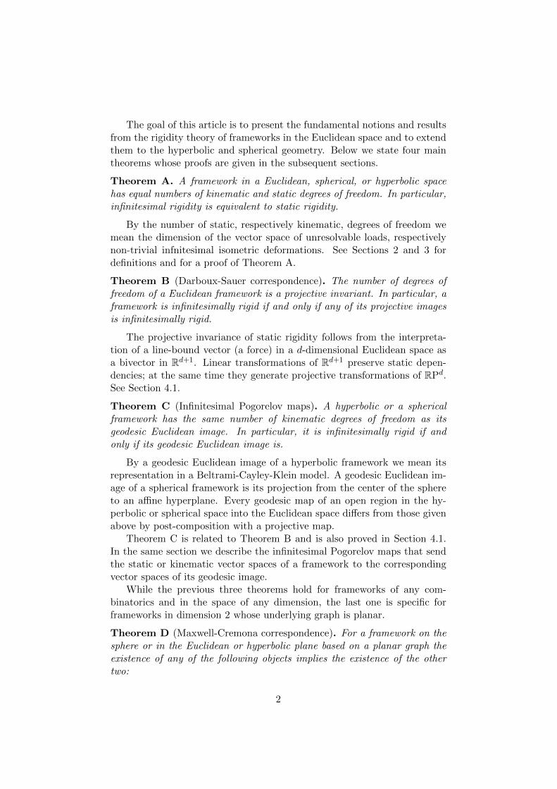
Definition 2.2. A framework (Γ, p) is called globally rigid, if every frame-work isometric to (Γ, p) is also congruent to it.
An isometric deformation of a framework (Γ, p) is a continuous familyof frameworks (Γ, p(t)) (i. e. every pi(t) is a continuous path in Xd), wheret ∈ (−ε, ε) and p(0) = p. An isometric deformation is called trivial, if it isgenerated by a family of ambient isometries: pi(t) = Φt(pi).
Definition 2.3. A framework (Γ, p) is called rigid (or locally rigid), if it hasno non-trivial isometric deformations. A non-rigid framework is also calledflexible.
Clearly, global rigidity implies rigidity, but not vice versa. See Figure 1.
Figure 1: Frameworks in the plane. Left: globally rigid. Middle: rigid butnot globally rigid. Right: flexible.
2.2 Infinitesimal motions
Definition 2.4. A vector field on a framework (Γ, p) is a map
q : Γ0 → TXd, i 7→ qi
such that qi ∈ TpiXd for all i. A vector field is called an infinitesimalisometric deformation of (Γ, p), if for some (and hence for every) smoothfamily of frameworks (Γ, p(t)) such that
p(0) = p,d
dt
∣∣∣∣t=0
pi(t) = qi for all i ∈ Γ0
4

we haved
dt
∣∣∣∣t=0
dist(pi(t), pj(t)) = 0
for all i, j ∈ Γ1.
Clearly, the infinitesimal isometry condition is equivalent to
〈qi, eij〉 − 〈qj , eji〉 = 0, (1)
where eij ∈ TpiXd is such that exppi(eij) = pj . We will rewrite this in adifferent way.
Lemma 2.5. A vector field q is an infinitesimal isometric deformation ofa framework (Γ, p) if and only if
〈pi − pj , qi − qj〉 = 0 in Ed;〈pi, qj〉+ 〈qi, pj〉 = 0 in Sd or Hd.
Here 〈pi, qj〉 means the Euclidean, respectively Minkowski scalar productin Rd+1, which makes sense if we identify TpiXd with a linear subspace ofRd+1.
Proof. This follows from (1) and
eij =
pj−pi‖pj−pi‖ in Ed;pj−〈pi,pj〉pi
sinX dist(pi,pj)in Sd and Hd.
An infinitesimal isometric deformation is called trivial, if there is a Killingfield K on Xd such that qi = K(pi) for all i.
Definition 2.6. A framework (Γ, p) is called infinitesimally rigid, if it hasno non-trivial infinitesimal isometric deformations.
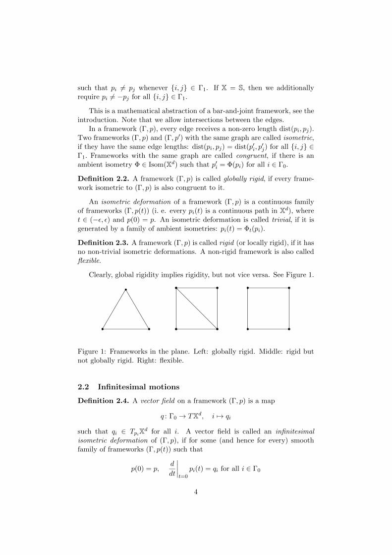
Theorem 2.7. An infinitesimally rigid framework is rigid.
For a proof, see [19, 2, 8].The converse of Theorem 2.7 is false, see Figure 2.Similarly to the example on Figure 2, one can construct a non-trivial in-
finitesimal isometric deformation for every framework contained in a geodesicsubspace of Xd (provided that the framework has at least 3 vertices). Thisis one of the reasons why it is convenient to consider only spanning frame-works: those whose vertices are not contained in a geodesic subspace.
Denote the set of all infinitesimal isometric deformations of a framework(Γ, p) by V (Γ, p). Due to Lemma 2.5, V (Γ, p) is a vector space. The set oftrivial infinitesimal isometric deformations is also a vector space; we denoteit by V0(Γ, p). If (Γ, p) is spanning, then dimV0(Γ, p) = d(d+1)
2 .
5
Figure 2: A rigid but infinitesimally flexible framework.
Definition 2.8. The dimension of the quotient space V (Γ, p)/V0(Γ, p) iscalled the number of kinematic degrees of freedom of a framework (Γ, p).
In particular, infinitesimally rigid frameworks are those with zero kine-matic degrees of freedom.
Remark 2.9. Determining whether a framework is flexible is more difficultthan determining whether it is infinitesimally flexible: the latter is a linearproblem, the former is an algebraic one. Examples of Bricard octahedra andKokotsakis polyhedra in Section 2.7 illustrate this.
2.3 Point-line frameworks
A point-line framework in R2 associates to every vertex i of Γ either a pointpi or a line li in R2. The edges of Γ correspond to the constraints of theform
dist(pi, pj) = dist(p′i, p′j), dist(pi, lj) = dist(p′i, l
′j), ∠(li, lj) = ∠(l′i, l
′j). (2)
For recent works on point-line frameworks see [27, 15].In the spherical geometry, a point-line framework is equivalent to a stan-
dard framework. If we replace every great circle by one of its poles, thenthe last two constraints in (2) take the form of the first one.
In the hyperbolic geometry, the pole of a line is a point in the de Sitterplane (the complement of the disk in the projective model of H2). Thereforethe study of point-line frameworks in H2 can be reduced to the study ofstandard frameworks in the hyperbolic-de Sitter plane. Moreover, we canallow ideal points, which means assigning horocycles to some of the verticesof Γ and fixing the point-horocycle, line-horocycle and horocycle-horocycledistances.
2.4 Constraints counting
One can estimate the dimension of the space of non-congruent realizationsof a framework by counting the constraints. If |Γ0| = n and |Γ1| = m,
6
then there are m equations on dn vertex coordinates. Besides, one has tosubtract the dimension of the space of trivial motions, which is d(d+1)
2 forspanning frameworks. Thus, generically a framework in Xd with n verticesand m edges has dn−m− d(d+1)
2 degrees of freedom.Of course, the above arithmetics does not make much sense without the
combinatorics (we can put a lot of edges on a subset of the vertices, allowingthe other vertices to fly away). Laman [30] has shown that in dimension 2the arithmetics and combinatorics suffice to characterize the generic rigidity.A graph Γ is called a Laman graph if |Γ1| = 2|Γ0| − 3 and every inducedsubgraph of Γ with k vertices has at most 2k − 3 edges.
Theorem 2.10. A Laman graph is generically rigid, that is the framework(Γ, p) is rigid for almost all p.
No analog of the Laman condition is known for frameworks in higherdimensions. See [10] for more details on the generic rigidity.
If all faces of a 3-dimensional polyhedron homeomorphic to a ball aretriangles, then its graph satisfies |Γ1| = 3|Γ0| − 6, that is the above countgives 0 as the upper bound for degrees of freedom. Rigidity of polyhedra isdiscussed in the next section.
2.5 Frameworks and polyhedra
One may try to generalize bar-and-joint frameworks by introducing panel-and-hinge structures: rigid polygons sharing pairs of sides and allowed tofreely rotate around these sides, or even more generally n-dimensional “pan-els” rotating around (n − 1)-dimensional “hinges”. A mathematical modelfor such an object is called a polyhedron or a polyhedral complex. However,there is a way to replace a polyhedral complex by a framework withoutchanging its isometric deformations (global as well as local and infinitesi-mal). For this, replace every panel by a complete graph on its vertex set.This “rigidifies” the panels and leaves them the freedom to rotate aroundthe hinges.
A particular class of polyhedral complexes are convex polyhedra. Ac-cording to the Legendre-Cauchy theorem [32, 7], a convex polyhedron isglobally rigid among convex polyhedra. There are simple examples of con-vex polyhedra isometric to non-convex ones. By the Dehn theorem [14](that can also be proved by the Legendre-Cauchy argument), convex 3-dimensional polyhedra are infinitesimally rigid.
The Legendre-Cauchy argument applies to spherical and hyperbolic con-vex polyhedra as well. This allows to prove the rigidity of convex polyhedrain Xd for d > 3 by induction: the link of a vertex of a d-dimensional convexpolyhedron is a (d − 1)-dimensional spherical polyhedron, and the rigidityof links implies the rigidity of the polyhedron.
7
A simplicial polyhedron (that is one all of whose faces are simplices) hasthe same kinematic properties as its 1-skeleton. In a convex non-simplicialpolyhedron we can replace every face by a complete graph as described inthe first paragraph; but in fact a much “lighter” framework is enough to keepthe polyhedron rigid. It suffices to triangulate every 2-dimensional face inan arbitrary way (without adding new vertices in the interior of the face,vertices on the edges are all right). Again, the Legendre-Cauchy argumentensures the rigidity of all 3-dimensional faces, and the induction applies asin the previous paragraph, [1, Chapter 10], [52].
As already indicated, the cone over a framework in Sd can be viewed asa panel structure (or a framework) in Ed+1. Similarly, a framework in Hd
leads to a framework in the (d+ 1)-dimensional Minkowski space.
2.6 Averaging and deaveraging
There is an elegant relation between the infinitesimal and global flexibility.(For smooth surfaces, this idea goes back to the 19th century.)
Theorem 2.11. 1) (Deaveraging.) Let (Γ, p) be a framework in Xd witha non-trivial infinitesimal isometric deformation q. Define two newframeworks (Γ, p+) and (Γ, p−) as follows.
p+i = pi + qi, p−i = pi − qi for X = E,
p+i =
pi + qi‖pi + qi‖
, p−i =pi − qi‖pi − qi‖
for X = S or H.
Then the frameworks (Γ, p+) and (Γ, p−) are isometric, but not con-gruent.
2) (Averaging.) Let (Γ, p′) and (Γ, p′′) be two isometric non-congruentframeworks in Xd. Put
pi =p′i + p′′i
2, qi =
p′i − p′′i2
for X = E,
pi =p′i + p′′i‖p′i + p′′i ‖
, qi =p′i − p′′i‖p′i + p′′i ‖
for X = S or H.
Then q is a non-trivial infinitesimal isometric deformation of (Γ, p).
In the deaveraging procedure it might happen that p+i = p+
j for some
i, j ∈ Γ1, so that p+ is not a framework. To avoid this, one can replace qby cq for a generic c ∈ R.
Proof. Formulas of the averaging are inverse to those of the deaveraging,and both statements can be proved by a direct calculation. Use that inthe spherical and the hyperbolic cases we have ‖pi + qi‖ = ‖pi − qi‖ due to〈pi, qi〉 = 0. Also q is non-trivial if and only if it changes the distance inthe first order between some pi and pj not connected by an edge. One cancheck that this is equivalent to dist(p+
i , p+j ) 6= dist(p−i , p
−j ).
8
2.7 Examples
In Section 2.4 we spoke about generically rigid graphs. The most interestingexamples of flexible frameworks are special realizations of generically rigidgraphs.
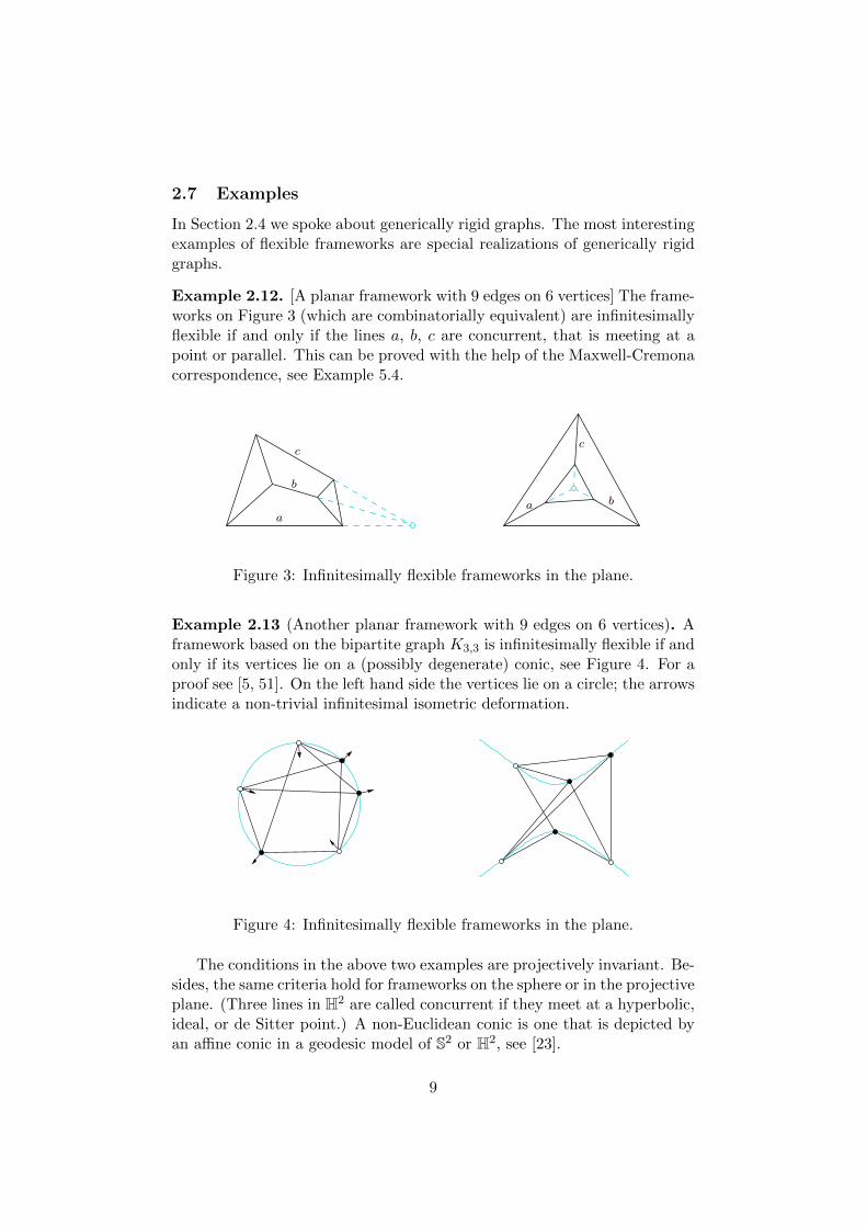
Example 2.12. [A planar framework with 9 edges on 6 vertices] The frame-works on Figure 3 (which are combinatorially equivalent) are infinitesimallyflexible if and only if the lines a, b, c are concurrent, that is meeting at apoint or parallel. This can be proved with the help of the Maxwell-Cremonacorrespondence, see Example 5.4.
a
b
c
a b
c
Figure 3: Infinitesimally flexible frameworks in the plane.
Example 2.13 (Another planar framework with 9 edges on 6 vertices). Aframework based on the bipartite graph K3,3 is infinitesimally flexible if andonly if its vertices lie on a (possibly degenerate) conic, see Figure 4. For aproof see [5, 51]. On the left hand side the vertices lie on a circle; the arrowsindicate a non-trivial infinitesimal isometric deformation.
Figure 4: Infinitesimally flexible frameworks in the plane.
The conditions in the above two examples are projectively invariant. Be-sides, the same criteria hold for frameworks on the sphere or in the projectiveplane. (Three lines in H2 are called concurrent if they meet at a hyperbolic,ideal, or de Sitter point.) A non-Euclidean conic is one that is depicted byan affine conic in a geodesic model of S2 or H2, see [23].
9

Example 2.14 (Bricard’s octahedra and Gaifullin’s cross-polytopes). Flex-ible octahedra (with intersecting faces) were discovered and classified byBricard [6], see also [49, 38]. A higher-dimensional analog of the octahe-dron is called cross-polytope. Recently, flexible cross-polytopes in Xd wereclassified by Gaifullin [18].
Example 2.15 (Infinitesimally flexible octahedra). While the descriptionand classification of flexible octahedra requires quite some work, infinitesi-mally flexible octahedra can be described in a simple and elegant way.
Color the faces of an octahedron white and black so that adjacentfaces receive different colors. An octahedron is infinitesimallyflexible if and only if the planes of its four white faces meet at apoint (which may lie at infinity). As a consequence, the planesof the white faces meet if and only if those of the black faces do.
This theorem was proved independently by Blaschke and Liebmann [4, 33].The configuration is related to the so called Mobius tetrahedra: a pair ofmutually inscribed tetrahedra, [37].
Figure 5 shows two examples of infinitesimally flexible octahedra. Theone on the left is a special case of the Schoenhardt octahedron [47]; its basesare regular triangles, and the orthogonal projection of one base to the othermakes the triangles concentric with pairwise perpendicular edges.
A
D
B
C
Figure 5: Infinitesimally flexible octahedra. On the right, the points A, B,C, D must be coplanar.
Theorem B implies that infinitesimally flexible octahedra in S3 and H3
are characterized by the same criterion as those in E3. In the hyperbolicspace, the intersection point of four planes may be ideal or hyperideal. Infact, even the vertices of an octahedron may be ideal or hyperideal. In-finitesimally flexible hyperbolic octahedra were used in [25] to constructsimple examples of infinitesimally flexible hyperbolic cone-manifolds.
10

Example 2.16 (Jessen’s icosahedron and its relatives). In the xy-plane ofR3, take the rectangle with vertices (±1,±, t, 0), where 0 < t < 1. Take twoother rectangles, obtained from this one by 120 and 240 rotations aroundthe x = y = z line (which results in cyclic permutations of the coordinates).The convex hull of the twelve vertices of these rectangles is an icosahedron
(a regular one for t =√
5−12 ). Among the edges of this icosahedron are the
short sides of the rectangles.Modify the 1-skeleton by removing the short sides of rectangles (like
the one joining (1, t, 0) with (1,−t, 0)) and inserting the long sides (like theone joining (1, t, 0) with (−1, t, 0)). The resulting framework p(t) is the 1-skeleton of a non-convex icosahedron. Jessen [28] gave the t = 1
2 non-convexicosahedron as an example of a closed polyhedron with orthogonal pairs ofadjacent faces, but different from the cube. See Figure 6.
Figure 6: Jessen’s orthogonal and infinitesimally flexible icosahedron.
The framework p(t) has two sorts of edges: the long sides of the rect-angles, which have length 2, and the sides of eight equilateral triangles,which have length
√2(t2 − t+ 1). It follows that the frameworks p(t) and
p(1− t) are isometric. Note that p(0) collapses to an octahedron: the mapp(t) : Γ0 → R3 sends the vertices of the icosahedral graph to the vertices ofa regular octahedron by identifying them in pairs; there are three pairs ofedges that are mapped to three diagonals of the octahedron. At the sametime, p(1) is the graph of the cuboctahedron with square faces subdividedin a certain way.
Since the average of p(t) and p(1− t) (in the sense of Section 2.6) is p(12),
it follows that Jessen’s icosahedron is infinitesimally flexible.Theorem B implies that there are spherical and hyperbolic analogs of
this construction.
Example 2.17 (Kokotsakis polyhedra). A Kokotsakis polyhedron with ann-gonal base is a panel structure made of a rigid n-gon, and n quadrilateralsattached to its edges, and n triangles attached between the quadrilaterals,
11
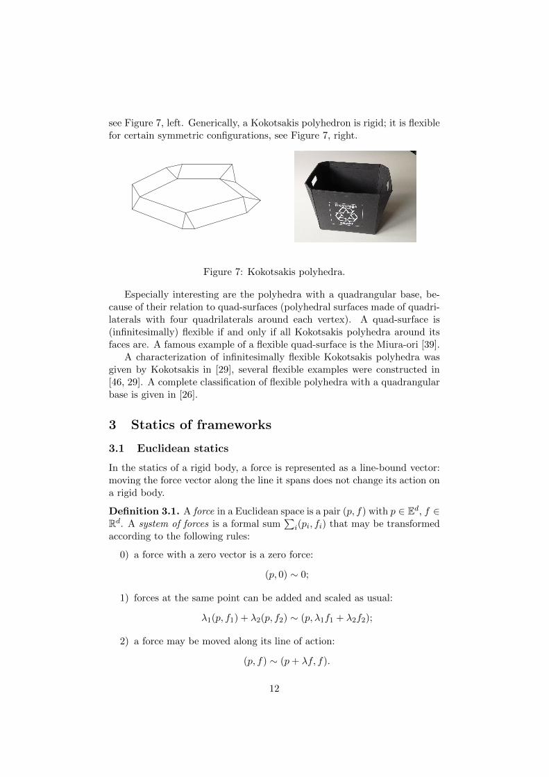
see Figure 7, left. Generically, a Kokotsakis polyhedron is rigid; it is flexiblefor certain symmetric configurations, see Figure 7, right.
Figure 7: Kokotsakis polyhedra.
Especially interesting are the polyhedra with a quadrangular base, be-cause of their relation to quad-surfaces (polyhedral surfaces made of quadri-laterals with four quadrilaterals around each vertex). A quad-surface is(infinitesimally) flexible if and only if all Kokotsakis polyhedra around itsfaces are. A famous example of a flexible quad-surface is the Miura-ori [39].
A characterization of infinitesimally flexible Kokotsakis polyhedra wasgiven by Kokotsakis in [29], several flexible examples were constructed in[46, 29]. A complete classification of flexible polyhedra with a quadrangularbase is given in [26].
3 Statics of frameworks
3.1 Euclidean statics
In the statics of a rigid body, a force is represented as a line-bound vector:moving the force vector along the line it spans does not change its action ona rigid body.
Definition 3.1. A force in a Euclidean space is a pair (p, f) with p ∈ Ed, f ∈Rd. A system of forces is a formal sum
∑i(pi, fi) that may be transformed
according to the following rules:
0) a force with a zero vector is a zero force:
(p, 0) ∼ 0;
1) forces at the same point can be added and scaled as usual:
λ1(p, f1) + λ2(p, f2) ∼ (p, λ1f1 + λ2f2);
2) a force may be moved along its line of action:
(p, f) ∼ (p+ λf, f).
12

One may check from this definition that systems of forces form a vectorspace of dimension d(d+1)
2 .In E2, any system of forces is equivalent either to a single force or to a
so called “force couple” (p1, f) + (p2,−f), where the vector f is not parallelto the line through p1 and p2.
Definition 3.2. A load on a Euclidean framework (Γ, p) is a map
f : Γ0 → Rd,i 7→ fi.
A load is called an equilibrium load if the system of forces∑
i∈Γ0(pi, fi) is
equivalent to a zero force.
A rigid body responds to an equilibrium load by interior stresses thatcancel the forces of the load. This motivates the following definition.
Definition 3.3. A stress on a framework (Γ, p) is a map
w : Γ1 → R,ij 7→ wij = wji.
The stress w is said to resolve the load f if
fi =∑j∈Γ0
wij(pj − pi) for all i ∈ Γ0, (3)
where we put wij = 0 for all ij /∈ Γ1.
We denote the vector space of equilibrium loads by F (Γ, p), and thevector space of resolvable loads by F0(Γ, p). It is easy to see that everyresolvable load is an equilibrium load: F0(Γ, p) ⊂ F (Γ, p).
Definition 3.4. The dimension of the quotient space F (Γ, p)/F0(Γ, p) iscalled the number of static degrees of freedom of the framework (Γ, p).
The framework (Γ, p) is called statically rigid if it has zero static degreesof freedom, i. e. if every equilibrium load can be resolved.
3.2 Non-euclidean statics
Definition 3.5. Let Xd = Sd or Hd. A force in Xd is an element of thetangent bundle TXd. We write it as a pair (p, f) with p ∈ Xd and f ∈ TpXd.
A system of forces is a formal sum of forces that may be transformedaccording to the rules of Definition 3.1, where the formula in the rule 2)is replaced by (p, f) ∼ (expp(λf), τ(f)) with τ(f) being the result of theparallel transport of f along the geodesic from p to expp(λf).
13
A system of forces on S2 is always equivalent to a single force; a systemof forces on H2 is equivalent to either a single force, or an ideal force coupleor a hyperideal force couple.
Definition 3.6. A load on a framework (Γ, p) in Xd is a map
f : Γ0 → TXd, fi ∈ TpiXd.
A load is called an equilibrium load if the system of forces∑
i∈Γ0(pi, fi) is
equivalent to a zero force.
In the above definitions, Xd can also stand for Ed. The canonical isomor-phisms TxEd ∼= Rd result in simplified formulations given in the precedingsection.
As in the Euclidean case, a stress on a framework in Xd is a map w : Γ1 →R. A stress w resolves a load f if
fi =∑j∈Γ0
wij dist(pi, pj)eij ,
where eij ∈ TpiXd is such that exppi(eij) = pj . The following lemma givesan alternative description of the stress resolution.
Lemma 3.7. A stress w resolves a load f on a framework (Γ, p) in Xd = Sdor Hd if and only if for every i ∈ Γ0 we have
fi −∑j∈Γ0
λijpj ‖ pi,
where λij = wijdist(pi,pj)
sinX dist(pi,pj). Here fi, pi ∈ Rd+1 via Xd ⊂ Rd+1.
Proof. Follows from the identity
pj − cosX dist(pi, pj)pi = pj − 〈pi, pj〉pi = sinX dist(pi, pj) · eij .
3.3 Equivalence of static and infinitesimal rigidity
Define a pairing between vector fields and loads on a framework (Γ, p):
〈q, f〉 =∑i∈Γ0
〈qi, fi〉. (4)
This pairing is non-degenerate and therefore induces a duality between thespace of vector fields and the space of loads.
Lemma 3.8 (Principles of virtual work). Under the pairing (4),
14
1) the space of infinitesimal motions is the annihilator of the space ofresolvable loads:
V (Γ, p) = F0(Γ, p);
2) the space of trivial infinitesimal motions is the annihilator of the spaceof equilibrium loads:
V0(Γ, p) = F (Γ, p).
A proof in the Euclidean case can be found in [24]; it transfers to thespherical and the hypebolic cases.
As a consequence, the pairing (4) induces an isomorphism
V (Γ, p)/V0(Γ, p) ∼= (F (Γ, p)/F0(Γ, p))∗ (5)
which implies Theorem A.The statics of a Euclidean framework is formulated in purely linear terms:
loads and stresses on a framework correspond to loads and stresses on itsaffine image. Together with Theorem A this leads to the following conclu-sion, which is a special case of Theorem B.
Corollary 3.9. The number of kinematic degrees of freedom of a Euclideanframework is an affine invariant. In particular, an affine image of an in-finitesimally rigid framework is infinitesimally rigid.
Definition 3.10. The rigidity matrix of a Euclidean framework (Γ, p) is aΓ1 × Γ0 matrix with vector entries:
R(Γ, p) = ij
i...
· · · pi − pj · · ·...
.
It has the pattern of the edge-vertex incidence matrix of the graph Γ, withpi − pj on the intersection of the row ij and the column i.
The rows of R(Γ, p) span the space F0(Γ, p). The following propositionis a reformulation of the first principle of virtual work.
Lemma 3.11. Consider R(Γ, p) as the matrix of a map (Rd)Γ0 → RΓ1.Then the following holds:
kerR(Γ, p) = V (Γ, p);imR(Γ, p)> = F0(Γ, p).
Corollary 3.12. A framework (Γ, p) is infinitesimally rigid if and only if
rkR(Γ, p) = d |Γ0| −(d+ 1
2
).
15
4 Projective statics and kinematics
4.1 Projective statics
For Xd = Ed, Sd or Hd associate to a force (p, f) in Xd a bivector in Rd+1:
(p, f) 7→ p ∧ f. (6)
We use the canonical embeddings Xd ⊂ Rd+1 that allow to view a point pand a vector f as vectors in Rd+1.
Lemma 4.1. The map (6) extends to an isomorphism between the space ofsystems of forces on Xd and the second exterior power Λ2(Rd+1).
The equivalence relations from Definition 3.1 ensure that a linear exten-sion is well-defined. For a proof of its bijectivity, see [24].
The above observation motivates the following definitions.
Definition 4.2. A projective framework is a graph Γ together with a map
π : Γ0 → RPd, i 7→ πi,
such that πi 6= πj for ij ∈ Γ1.
We say that φ ∈ Λ2(Rd+1) is divisible by a vector v, if φ = v∧w for somevector w. Similarly, we say that φ is divisible by π ∈ RPd, if φ is divisibleby a representative of π.
Definition 4.3. A load on a projective framework (Γ, π) is a map
φ : Γ0 → Λ2(Rd+1), i 7→ φi,
that sends every vertex i to a bivector divisible by πi. An equilibrium loadis one that satisfies ∑
i∈Γ0
φi = 0.
Definition 4.4. Denote by Γor1 the set of oriented edges of the graph Γ. A
stress on a projective framework (Γ, π) is a map
Ω: Γor1 → Λ2(Rd+1), (i, j) 7→ ωij
such that ωij is divisible by both πi and πj , and ωij = −ωji.A stress Ω is said to resolve a load φ if
φi =∑j∈Γ0
ωij .
The projectivization of a framework (Γ, p) in Xd is obtained by composingp with the inclusion Xd ⊂ Rd+1 and the projection Rd+1 \ 0 → RPd. Thefollowing lemma is straightforward.
16
Lemma 4.5. The map (6) sends bijectively the equilibrium, respectivelyresolvable, loads on a framework in Xd to the equilibrium, respectively re-solvable, loads on its projectivization.
Theorems B and C are immediate corollaries of Lemma 4.5.
Proof of Theorem B. Two frameworks in Ed are projective images of oneanother if and only if their projectivizations are related by a linear isomor-phism of Rd+1. A linear map sends equilibrium loads to equilibrium ones,and resolvable to resolvable ones.
It seems that Theorem B was first proved by Rankine [43] in 1863. Hestated that the static rigidity is projective invariant but did not give thedetails, just saying that “... theorems discovered by Mr. Sylvester ... obvi-ously give at once the solution of the question”. The first detailed accountsare [33] (for a special case |Γ1| = d|Γ0| − d(d+1)
2 ) and [45].
Proof of Theorem C. A Euclidean framework and its geodesic spherical orhyperbolic image have the same projectivizations. Hence the maps (6) yieldan isomorphism between the spaces of their equilibrium/resolvable loads.
4.2 Static and kinematic Pogorelov maps
Let a framework (Γ, p) in Ed and a projective map Φ: RPd → RPd begiven such that the image of Φ p is contained in Ed. (Here RPd is aprojective completion of Ed). Lemma 4.5 does not only show that the spacesof equilibrium modulo resolvable loads of (Γ, p) and (Γ,Φp) have the samedimension, but also establishes a canonical up to a scalar factor isomorphismbetween these spaces. Through the static-kinematic duality from Section3.3 this also yields an isomorphism between the spaces of infinitesimallyisometric modulo trivial motions.
The situation is similar with the geodesic correspondence between frame-works in different geometries. The kinematic isomorphisms were describedby Pogorelov in [41, Chapter 5] together with the maps that associate to apair of isometric polyhedra in one geometry a pair of isometric polyhedrawith the same combinatorics in the other geometry (related to the kinematicisomorphism via the averaging procedure, see Section 2.6). We will use theterm Pogorelov maps in each of the above situations.
Definition 4.6. Let X ⊂ Xd and Y ⊂ Yd, where X,Y ∈ E, S,H, and letΦ: X → Y be a geodesic map. A fiberwise linear map Φstat : TX → TYwith Φstat(TpX) ⊂ TΦ(p)Y is called a static Pogorelov map associated with Φif for every framework (Γ, p) in X the following two conditions are satisfied:
• a load f on (Γ, p) is in equilibrium if and only if the load Φstat f onthe framework (Γ,Φ p) is in equilibrium;
17
• a load f on (Γ, p) is resolvable if and only if the load Φstat f on theframework (Γ,Φ p) is resolvable.
A fiberwise linear map Φkin : TX → TY with Φkin(TpX) ⊂ TΦ(p)Y iscalled a kinematic Pogorelov map associated with Φ if for every framework(Γ, p) in X the following two conditions are satisfied:
• a vector field q on (Γ, p) is an infinitesimal isometric deformation ifand only if the vector field Φkin q on (Γ,Φ p) is an infinitesimalisometric deformation;
• a vector field q on (Γ, p) is a trivial infinitesimal isometric deformationif and only if the vector field Φkinq on (Γ,Φp) is a trivial infinitesimalisometric deformation.
Remark 4.7. The last condition on a kinematic Pogorelov map means thatΦkin sends Killing fields on X to Killing fields on Y . For an intrinsic ap-proach to the Pogorelov maps defined for Riemannian metrics with the samegeodesics, see [17, Section 4.3].
Lemma 4.8. If Φstat is a static Pogorelov map associated with Φ, then((Φstat)−1)∗ is a kinematic Pogorelov map associated with Φ.
Proof. Follows from
〈((Φstat)−1)∗(q),Φstat(f)〉 = 〈q, (Φstat)−1 Φstat(q)〉 = 〈q, f〉
and from Lemma 3.8.
4.3 Pogorelov maps for affine and projective transformations
Theorem 4.9. Let Φ: Ed → Ed be an affine transformation with the linearpart A = dΦ ∈ GL(n,R). Then
Φstat = A, Φkin = (A−1)∗
are static and kinematic Pogorelov maps for Φ.
Proof. Equivalence relation in Definition 3.1 is affinely invariant. Thereforef is an equilibrium load on (Γ, p) if and only if A f is an equilibrium loadon (Γ,Φ p). When (Γ, p) is transformed by Φ, the right hand side of (3) istransformed by A. Therefore a stress that resolves f also resolves A f .
Theorem 4.10. LetΦ: Ed \ L→ Ed \ L′
be a projective transformation, where L is the hyperplane sent to infinity, andL′ is the image of the hyperplane at infinity. Denote by hL(p) the distancefrom a point p ∈ Ed to the hyperplane L. Then
Φstatp = h2
L(p) · dΦp, Φkinp = h−2
L (p) · ((dΦp)∗)−1
are static and kinematic Pogorelov maps for Φ.
18
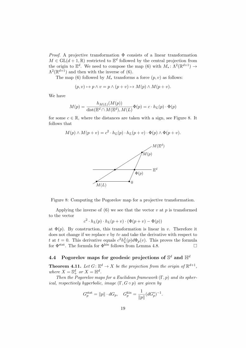
Proof. A projective transformation Φ consists of a linear transformationM ∈ GL(d + 1,R) restricted to Ed followed by the central projection fromthe origin to Ed. We need to compose the map (6) with M∗ : Λ2(Rd+1) →Λ2(Rd+1) and then with the inverse of (6).
The map (6) followed by M∗ transforms a force (p, v) as follows:
(p, v) 7→ p ∧ v = p ∧ (p+ v) 7→M(p) ∧M(p+ v).
We have
M(p) =hM(L)(M(p))
dist(Ed ∩M(Ed),M(L)Φ(p) = c · hL(p) · Φ(p)
for some c ∈ R, where the distances are taken with a sign, see Figure 8. Itfollows that
M(p) ∧M(p+ v) = c2 · hL(p) · hL(p+ v) · Φ(p) ∧ Φ(p+ v).
0
M(p)
M(L)
M(Ed)
Φ(p)Ed
Figure 8: Computing the Pogorelov map for a projective transformation.
Applying the inverse of (6) we see that the vector v at p is transformedto the vector
c2 · hL(p) · hL(p+ v) · (Φ(p+ v)− Φ(p))
at Φ(p). By construction, this transformation is linear in v. Therefore itdoes not change if we replace v by tv and take the derivative with respect tot at t = 0. This derivative equals c2h2
L(p)dΦp(v). This proves the formulafor Φstat. The formula for Φkin follows from Lemma 4.8.
4.4 Pogorelov maps for geodesic projections of Sd and Hd
Theorem 4.11. Let G : Ed → X be the projection from the origin of Rd+1,where X = Sd+ or X = Hd.
Then the Pogorelov maps for a Euclidean framework (Γ, p) and its spher-ical, respectively hyperbolic, image (Γ, G p) are given by
Gstatp = ‖p‖ · dGp, Gkin
p =1
‖p‖(dG∗p)
−1.
19
Here ‖ · ‖ denotes the Euclidean, respectively Minkowski, norm in Rd+1.
Note that in the spherical case at the point e0 (the tangency point ofX with Ed) we have Gstat
e0 = dGe0 . In the hyperbolic case we have Gstate0 =
−dGe0 , so one might want to change the sign in the formulas.
p tv
t · dGp(v)
v
Gstatp (v)
p
G(p) G(p)
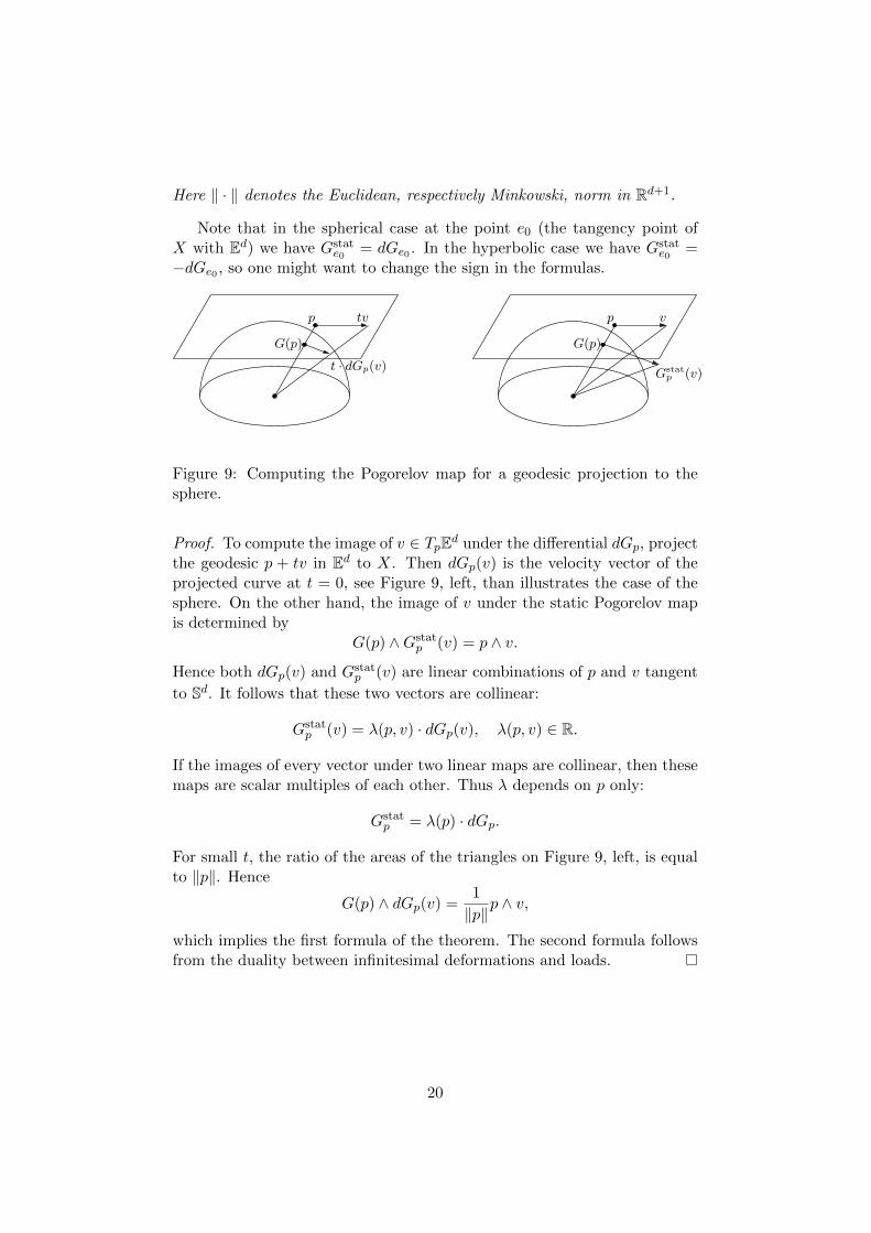
Figure 9: Computing the Pogorelov map for a geodesic projection to thesphere.
Proof. To compute the image of v ∈ TpEd under the differential dGp, projectthe geodesic p + tv in Ed to X. Then dGp(v) is the velocity vector of theprojected curve at t = 0, see Figure 9, left, than illustrates the case of thesphere. On the other hand, the image of v under the static Pogorelov mapis determined by
G(p) ∧Gstatp (v) = p ∧ v.
Hence both dGp(v) and Gstatp (v) are linear combinations of p and v tangent
to Sd. It follows that these two vectors are collinear:
Gstatp (v) = λ(p, v) · dGp(v), λ(p, v) ∈ R.
If the images of every vector under two linear maps are collinear, then thesemaps are scalar multiples of each other. Thus λ depends on p only:
Gstatp = λ(p) · dGp.
For small t, the ratio of the areas of the triangles on Figure 9, left, is equalto ‖p‖. Hence
G(p) ∧ dGp(v) =1
‖p‖p ∧ v,
which implies the first formula of the theorem. The second formula followsfrom the duality between infinitesimal deformations and loads.
20

5 Maxwell-Cremona correspodence
5.1 Planar 3-connected graphs, polyhedra, and duality
A graph is called 3-connected if it is connected, has at least 4 vertices, andremains connected after removal of any two of its vertices. In particular,every vertex of a 3-connected graph has degree at least 3.
Planar 3-connected graphs have very nice properties. First, by a resultof Whitney [54], their embeddings into S2 split in two isotopy classes thatdiffer by an orientation-reversing diffeomorphism of S2. Second, by theSteinitz theorem [50, 55], a graph is planar and 3-connected if and only ifit is isomorphic to the skeleton of some convex 3-dimensional polyhedron.Whitney’s theorem implies that for a planar 3-connected graph Γ there is awell-defined set of faces Γ2. Geometrically, a face is a connected componentof S2 \ φ(Γ), where φ is an embedding of Γ; combinatorially it is the set ofvertices on the boundary of such a component. We call (α, i) with α ∈ Γ2,i ∈ Γ0 and i ∈ α an incident pair. Choice of an isotopy class of an embeddingΓ→ S2 and of an orientation of S2 induces a cyclic order on the set of verticesincident to a face.
The dual graph Γ∗ of a planar 3-connected graph Γ can be constructedfrom an embedding Γ→ S2 by choosing a point inside every face and joiningevery pair of points whose corresponding faces share an edge. The graph Γ∗
is also planar and 3-connected, and its dual is again Γ. If an edge ij of Γseparates the faces α and β, then we say that (αβ, ij) is a dual pair of edges.Choose an isotopy class of embeddings Γ→ S2 and fix an orientation of S2.Then we say that the pair (αβ, ij) is consistently oriented if the face α lieson the right from the edge ij directed from i to j, see Figure 10. Changingthe order of i and j or of α and β transforms an inconsistently oriented pairinto a consistently oriented one.
i
j
α
β
Figure 10: A consistently oriented dual pair.
5.2 Maxwell-Cremona theorem
For convenience we identify in this section E2 with R2 by choosing an origin.
21
Definition 5.1. Let (Γ, p) be a framework in R2 with a planar 3-connectedgraph Γ. A reciprocal diagram for (Γ, p) is a framework (Γ∗,m) such thatdual edges are perpendicular to each other:
mβ −mα ⊥ pj − pi
whenever the edge ij of Γ separates the faces α and β.
Definition 5.2. Let (Γ, p) be a framework in R2 with a planar 3-connectedgraph Γ and such that for every face α ∈ Γ2 the points pi | i ∈ α are notcollinear. A vertical polyhedral lift of (Γ, p) is a map p : Γ0 → R3 such that
1) pr⊥ p = p, where pr⊥ : R3 → R2 is the orthogonal projection;
2) for every face α of (Γ, p) the points pi | i ∈ α are coplanar;
3) the planes of the adjacent faces differ from each other.
A radial polyhedral lift of (Γ, p) is a map p : Γ0 → R3 that satisfies the aboveconditions with 1) replaced by
1’) pra p = p, where pra : R3 \ a → R2 is the radial projection from apoint a /∈ R2.
It turns out that reciprocal diagrams are related to polyhedral lifts andto the statics of the framework (Γ, p).
A stress w : Γ1 → R on a framework (Γ, p) is called a self-stress if itresolves the zero load:∑
j∈Γ0
wij(pj − pi) = 0 for all i ∈ Γ0. (7)
Theorem 5.3. Let (Γ, p) be a framework in R2 with a planar 3-connectedgraph Γ and such that for every face α ∈ Γ2 the points pi | i ∈ α are notcollinear. Then the following conditions are equivalent:
1) The framework has a self-stress that is non-zero on all edges.
2) The framework has a reciprocal diagram.
3) The framework has a vertical polyhedral lift.
4) The framework has a radial polyhedral lift.
Proof. 1) ⇒ 2): From a self-stress w construct a reciprocal diagram (Γ∗,m)in the following recursive way. Take any face α0 and define mα0 ∈ R2
arbitrarily. If for some face α the point mα is already defined, then forevery β adjacent to α put
mβ = mα + wijJ(pj − pi),
22

where J : R2 → R2 is the rotation by the angle π2 , ij is the edge dual to
αβ, and the pair (αβ, ij) is consistently oriented. In order to show thatthis gives a well-defined map m : Γ2 → R2, we need to check that the sum∑
ij wijJ(pj−pi) vanishes along every closed path in the graph Γ∗. Viewed asa simplicial chain, every closed path is a sum of paths around vertices. Thesum around a vertex vanishes due to (7). By construction, mβ−mα ⊥ pj−piandmα 6= mβ for α and β adjacent in Γ∗, thus (Γ∗,m) is a reciprocal diagramfor (Γ, p).
2) ⇒ 1): Let (αβ, ij) be a consistently oriented dual pair. Since mβ −mα ⊥ pj − pi, there is wij ∈ R such that mβ −mα = wijJ(pj − pi). Themap w : Γ1 → R thus constructed never vanishes and satisfies (7).
3) ⇒ 2): Given a polyhedral lift of (Γ, p), let Mα ⊂ R3 be the plane towhich the face α is lifted. Since Mα is not vertical, it is the graph of a linearfunction fα : R2 → R. Put mα = grad fα. For every dual pair (αβ, ij) wehave
pi, pj ∈Mα ∩Mβ.
This implies that the linear function fα−fβ vanishes along the line throughpi and pj , hence
mα −mβ = grad(fα − fβ) ⊥ pi − pj .
2) ⇒ 3): Given a reciprocal diagram (Γ∗,m), construct a polyhedral liftrecursively. Take any α0 and let fα0 : R2 → R be any linear function withgrad fα0 = mα0 . If fα is defined for some α, then define fβ for every βadjacent to α by requiring
grad fβ = mβ, fβ − fα = 0 on the line pipj ,
where ij is the edge dual to αβ. These conditions are consistent due tomβ −mα ⊥ pj − pi. In order to check that the recursion is well-defined, itsuffices to show that if we start with some fα and apply the recursion aroundthe vertex i ∈ α, then the new fα will be the same as the old one. Thisis indeed the case because by construction all fβ with i ∈ β take the samevalue at pi. A polyhedral lift of (Γ, p) is obtained by putting pi = fα(pi) forany α 3 i.
3) ⇔ 4): Consider R3 as an affine chart of RP3. There is a projectivetransformation Φ: RP3 → RP3 that restricts to the identity on R2 ⊂ R3
and sends the point a to the point at infinity that corresponds to the pencilof lines perpendicular to R2. (This transformation exchanges the plane atinfinity with the plane through a parallel to R2.) We have pra = pr⊥ Φ.Therefore if p is a radial polyhedral lift of p, then Φ p is an orthogonal liftof p. Conversely, if p is an orthogonal lift such that pi does not lie on theplane through a parallel to R2, then Φ−1 : p is a radial lift. Any orthogonallift can be shifted in the direction orthogonal to R2 so that its vertices don’t
23
lie on the plane through a parallel to R2. Therefore the existence of anorthogonal lift is equivalent to the existence of a radial lift.
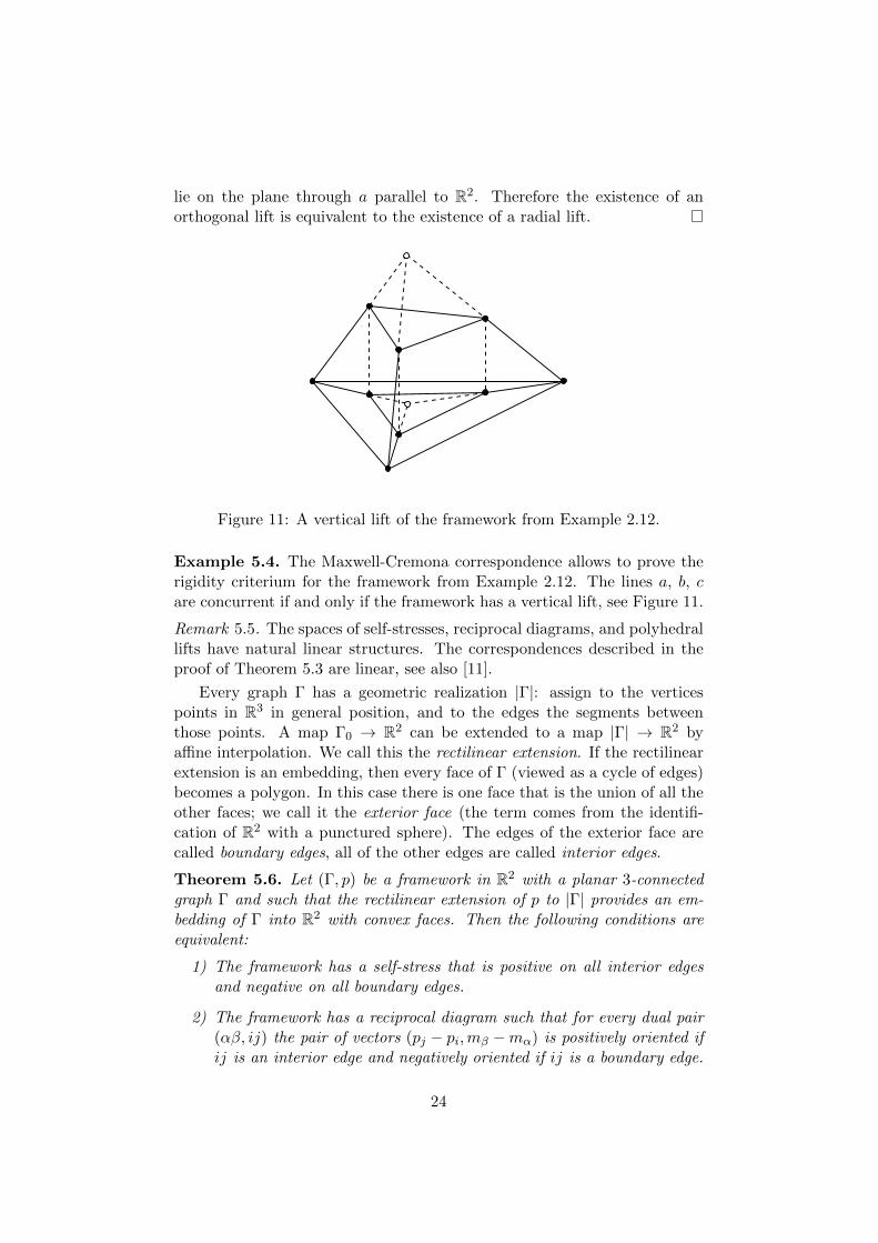
Figure 11: A vertical lift of the framework from Example 2.12.
Example 5.4. The Maxwell-Cremona correspondence allows to prove therigidity criterium for the framework from Example 2.12. The lines a, b, care concurrent if and only if the framework has a vertical lift, see Figure 11.
Remark 5.5. The spaces of self-stresses, reciprocal diagrams, and polyhedrallifts have natural linear structures. The correspondences described in theproof of Theorem 5.3 are linear, see also [11].
Every graph Γ has a geometric realization |Γ|: assign to the verticespoints in R3 in general position, and to the edges the segments betweenthose points. A map Γ0 → R2 can be extended to a map |Γ| → R2 byaffine interpolation. We call this the rectilinear extension. If the rectilinearextension is an embedding, then every face of Γ (viewed as a cycle of edges)becomes a polygon. In this case there is one face that is the union of all theother faces; we call it the exterior face (the term comes from the identifi-cation of R2 with a punctured sphere). The edges of the exterior face arecalled boundary edges, all of the other edges are called interior edges.
Theorem 5.6. Let (Γ, p) be a framework in R2 with a planar 3-connectedgraph Γ and such that the rectilinear extension of p to |Γ| provides an em-bedding of Γ into R2 with convex faces. Then the following conditions areequivalent:
1) The framework has a self-stress that is positive on all interior edgesand negative on all boundary edges.
2) The framework has a reciprocal diagram such that for every dual pair(αβ, ij) the pair of vectors (pj − pi,mβ −mα) is positively oriented ifij is an interior edge and negatively oriented if ij is a boundary edge.
24
3) The framework has a vertical polyhedral lift to a convex polytope.
4) The framework has a radial polyhedral lift to a convex polytope.
Proof. It suffices to show that the constructions in the proof of Theorem 5.3respect the above properties.
1) ⇔ 2): Since a self-stress is related to a reciprocal diagram by theformula mβ −mα = wijJ(pj − pi), the pair (pj − pi,mβ −mα) is positivelyoriented if and only if wij > 0.
2) ⇔ 3): Since mβ −mα = grad(fβ − fα), the pairs (pj − pi,mβ −mα)for all interior edges ij are positively oriented if and only if the piecewiselinear function over the union of the interior faces defined by f(x) = fα(x)for x ∈ α is convex. The graph of this function together with the lift ofthe exterior face (that covers the union of the interior faces) form a convexpolytope.
3) ⇔ 4): The projective image of a convex polytope (provided no pointis sent to infinity) is a convex polytope. The orthogonal lift can be madedisjoint from the plane that is sent to infinity by shifting in the verticaldirection.
Remark 5.7. By adding a linear function to an orthogonal polyhedral liftwe can achieve that the exterior face stays in R2. A convex polytope of thiskind is called a convex cap. An example is given on Figure 11.
Remark 5.8. The only self-intersections of the reciprocal diagram from The-orem 5.6 involve the edges mα0mβ, where α0 is the exterior face of Γ (andthere is no way to get rid of all self-intersections unless Γ is the graph ofthe tetrahedron). The reciprocal diagram can be represented without self-intersections by replacing every edge mα0mβ with a ray running from mβ inthe direction opposite to mα0 . Complexes of this sort are called spider websin [53].
Non-crossing frameworks with non-crossing reciprocals (and thus withsome non-convex faces) are studied in the article [40].
Remark 5.9. The Dirichlet tesselation of a finite point set and the corre-sponding Voronoi diagram are a special case of a framework and a reciprocaldiagram of the type described in Theorem 5.6. The vertical lift is given bypi = (pi, ‖pi‖2). The Voronoi diagram represents the reciprocal in the formof a spider web as described in the previous remark. A generalization ofDirichlet tesselations and Voronoi diagrams are weighted Delaunay tessela-tions and power diagrams. One of the definitions of a weighted Delaunaytesselation is a tesselation that possesses a vertical lift to a convex polytope.Thus one can a fifth equivalent condition to Theorem 5.6: the framework isa weighted Delaunay tesselation. For details see [3].
In [53] the spider webs were related to planar sections of spatial Delaunaytesselations.
25

Remark 5.10. Not every convex tesselation and even not every triangulationof a convex polygon has a convex polyhedral lift, see [13, Chapter 7.1] for the“mother of all counterexamples”. Those that do are called coherent or reg-ular triangulations (more generally, tesselations). There is a generalizationto higher dimensions, see [13].
5.3 Maxwell-Cremona correspondence in spherical geometry
Definition 5.11. Let (Γ, p) be a framework in S2 with a planar 3-connectedgraph Γ. A weak reciprocal diagram for (Γ, p) is a framework (Γ∗,m) in S2
such that
1) for every dual pair (αβ, ij) the geodesics pipj and mαmβ are perpen-dicular;
2) for every incident pair (α, i) the distance between mα and pi is differentfrom π
2 .
A strong reciprocal diagram is defined in the same way except that condition2) is replaced by
2’) for every incident pair (α, i) the distance between mα and pi is lessthan π
2 .
The reciprocity conditions can be rewritten as
〈mα, pi〉〈mβ, pj〉 − 〈mα, pj〉〈mβ, pi〉 = 0 (8)
〈mα, pi〉 6= 0 (9)
〈mα, pi〉 > 0 (9’)
The left hand side in (8) equals 〈mα ×mβ, pi × pj〉.
Definition 5.12. Let (Γ, p) be a framework in S2 with a planar 3-connectedgraph Γ and such that for every face α ∈ Γ2 the points pi | i ∈ α are notcollinear (that is, don’t lie on a great circle). A weak polyhedral lift of (Γ, p)is a map p : Γ0 → R3 such that
1) pi = aipi for every i ∈ Γ0, where ai 6= 0;
2) for every face α ∈ Γ2 the points pi | i ∈ α are coplanar;
3) the planes of the adjacent faces differ from each other.
A strong polyhedral lift is defined similarly but with ai > 0 in condition 1.
Theorem 5.13. Let (Γ, p) be a framework in S2 with a planar 3-connectedgraph Γ and such that for every face α ∈ Γ2 the points pi | i ∈ α are notcollinear. Then the following conditions are equivalent:
26
1) The framework has a self-stress that is non-zero on all edges.
2) The framework has a weak reciprocal diagram.
3) The framework has a weak polyhedral lift.
Proof. 1)⇒ 3): By Lemma 3.7, a self-stress w gives rise to a map λ : Γ1 → Rsuch that ∑
j∈Γ0
λijpj ‖ pi for all i ∈ Γ0. (10)
Pick an α0 ∈ Γ2 and define mα0 ∈ R3 arbitrarily. Define m : Γ2 → R3
recursively: if mα is already defined, then for every β adjacent to α put
mβ = mα + λij(pi × pj),
where (αβ, ij) is a consistently oriented dual pair. Equation (10) impliesthat the closing condition around every vertex i holds:∑
j
λij(pi × pj) = 0.
Thus we have a well-defined map m : Γ2 → R3 with
mβ − mα ‖ pi × pj
for any dual pair (αβ, ij). In particular, mβ − mα ⊥ pi, which implies thatfor every i there is ci ∈ R such that
〈mα, pi〉 = ci
for all α incident to i. For a generic initial choice of mα0 we have ci 6= 0 forall i. If we put pi = pi
ci, then we have
〈mα, pi〉 = 1
for every incident pair (α, i). It follows that for every α ∈ Γ2 the pointspi | i ∈ α are coplanar and span a plane orthogonal to the vector mα.Due to λij 6= 0 for every edge ij the planes of adjacent faces are different,thus we have constructed a weak polyhedral lift of (Γ, p).
3) ⇒ 2): Let Mα ⊂ R3 be the plane containing the points pi | i ∈ α.Since the points pi | i ∈ α are not collinear, the plane Mα does not passthrough the origin. Thus it has equation of the form
Mα = x ∈ R3 | 〈mα, x〉 = 1
for some mα ∈ R3. In particular, for any dual pair (αβ, ij) we have
〈mβ − mα, pi〉 = 〈mβ − mα, pj〉 = 0.
27
Hence the vector mβ− mα, and with it the plane spanned by mα and mβ, isperpendicular to the plane spanned by pi and pj . If we put mα = mα
‖mα‖ , then
the geodesic mαmβ is perpendicular to the geodesic pipj . Since 〈mα, pi〉 = 1,we have 〈mα, pi〉 6= 0. Thus (Γ∗,m) is a weak reciprocal diagram to (Γ, p).
2) ⇒ 3): Let (Γ∗,m) be a weak reciprocal diagram for (Γ, p). We con-struct lifts m and p such that
〈mα, pi〉 = 1 (11)
for every incident pair (α, i). The construction is recursive.Pick α0 ∈ Γ2 and lift mα0 arbitrarily. Due to (9), for every i ∈ α0 there
is a lift pi of pi such that 〈mα0 , pi〉 = 1. If mα is already defined, and β isadjacent to α, then let ij be the edge dual to αβ. First determine the liftpi from the condition (11), and then determine the lift mβ from the samecondition with β in place of α. Note that if we use pj instead of pi, thenthe result will be the same: due to the reciprocity conditions (8) and (9) wehave
〈mα, pi〉 = 〈mα, pj〉 ⇒ 〈mβ, pi〉 = 〈mβ, pj〉.
This recursive procedure leads to well-defined lifts m and p: going arounda vertex i does not change the value of mα because both the initial and thefinal values satisfy (11).
3) ⇒ 1): Let m : Γ2 → R3 be the map constructed during the proof ofthe implication 3) ⇒ 2). As it was shown, for every dual pair (αβ, ij) thenon-zero vector mβ−mα is perpendicular to pi and pj . Thus we have a mapλ : Γ1 → R such that
mβ − mα = λijpi × pj .
To determine the sign of λij , we order the vertices so that the pair (αβ, ij)is consistently oriented. Summing around a vertex i of Γ we obtain
pi ×∑j∈Γ0
λijpj = 0.
Hence∑
j∈Γ0λijpj ‖ pi and by Lemma 3.7 the map λ gives rise to a non-zero
self-stress on (Γ, p).
We don’t know what conditions on a framework and the stress guaranteethe existence of a strong reciprocal diagram. At least it is necessary that thevertices of every face are contained in an open hemisphere. The next theoremshows that strong reciprocal diagrams correspond to strong polyhedral lifts.
Theorem 5.14. Let (Γ, p) be a framework in S2 as in Theorem 5.13. Thenthe following conditions are equivalent:
1) The framework has a strong reciprocal diagram.
28
2) The framework has a strong polyhedral lift.
Proof. In the proof of 3) ⇒ 2) in Theorem 5.13, note that for a strong liftp the equation 〈mα, pi〉 = 1 implies 〈mα, pi〉 > 0, so that the reciprocaldiagram constructed from a strong lift is strong itself.
In the proof of 2)⇒ 3) in Theorem 5.13, lift mα0 strongly (that is scale itby a positive factor). Condition (11) implies that all pi with i ∈ α0 are alsolifted strongly. The recursion propagates the strong lift to all mβ and pj .
As in the Euclidean case (see the paragraph before Theorem 5.6), aspherical framework defines a geodesic extension, that is a map |Γ| → S2
that sends every edge to an arc of a great circle. A geodesic extension iscalled a convex embedding of Γ if it is an embedding and every face is aconvex spherical polygon.
Theorem 5.15. Let (Γ, p) be a framework in S2 with a planar 3-connectedgraph Γ and such that its geodesic extension is a convex embedding. Thenthe following conditions are equivalent:
1) The framework has a self-stress that is positive on all edges.
2) The framework has a strong reciprocal diagram that embeds Γ∗ in S2
with convex faces.
3) The framework has a strong lift to a convex polyhedron.
Proof. 1) ⇒ 3): In the proof of the corresponding implication in Theorem5.13 we have λij > 0 for all edges ij. This implies that as we go arounda vertex i, the vertices mα for all α adjacent to i form a convex polygon.The union of these polygons is the boundary of a convex polyhedron thatcontains 0 in its interior. Its polar dual is a strong lift of (Γ, p).
3)⇒ 2): A convex polyhedron that is a strong lift of (Γ, p) contains 0 inthe interior. Thus its polar dual is also a convex polyhedron. The projectionof the 1-skeleton of the dual is a strong reciprocal diagram with convex faces.
2) ⇒ 1): In a strong reciprocal diagram with convex faces the geodesicsmαmβ and pipj that correspond to a dual pair are consistently oriented.When we lift such a diagram as in the proof of 2) ⇒ 3) ⇒ 1) in Theorem5.13, we obtain real numbers λij > 0 that provide a positive self-stress on(Γ, p).
The latter version of the spherical Maxwell-Cremona correspondence wasdescribed in [34].
Remark 5.16. As in the Euclidean case, not every convex tesselation of thesphere has a convex polyhedral lift. The corresponding theory predates thetheory of regular triangulations in the Euclidean space and was developedby Shephard [48] and McMullen [35]. See also [16].
29
5.4 Maxwell-Cremona correspondence in hyperbolic geome-try
Let (Γ, p) be a framework in H2 with a planar 3-connected graph Γ. Areciprocal diagram is a framework (Γ∗,m) in H2 such that for every dualpair (αβ, ij) the geodesics mαmβ and pipj are perpendicular. In terms ofthe Minkowski scalar product this means
〈mα, pi〉〈mβ, pj〉 − 〈mα, pj〉〈mβ, pi〉 = 0.
Remark 5.17. The above criterion of orthogonality of mαmβ and pipj aswell as its spherical analog (8) can be reformulated as follows. Diagonals ina spherical or hyperbolic quadrilateral with the side lengths a, b, c, d in thiscyclic order are orthogonal if and only if
cosX a cosX c = cosX b cosX d.
The diagonals of a Euclidean quadrilateral are orthogonal if and only ifa2 + c2 = b2 + d2.
Definition 5.18. Let (Γ, p) be a framework in H2 with a planar 3-connectedgraph Γ and such that for every face α ∈ Γ2 the points pi | i ∈ α are notcollinear. A polyhedral lift of (Γ, p) is a map p : Γ0 → R3 such that
1) pi = aipi for every i ∈ Γ0, where ai > 0;
2) for every face α ∈ Γ2 the points pi | i ∈ α are contained in a space-like plane;
3) the planes of the adjacent faces differ from each other.
Theorem 5.19. Let (Γ, p) be a framework in H2 with a planar 3-connectedgraph Γ and such that for every face α ∈ Γ2 the points pi | i ∈ α are notcollinear. Then the following conditions are equivalent:
1) The framework has a self-stress that is non-zero on all edges.
2) The framework has a reciprocal diagram.
3) The framework has a polyhedral lift.
Proof. 1) ⇒ 3): Proceed as in the proof of Theorem 5.13 to obtain a mapm : Γ2 → R3 such that
mβ − mα ‖ pi × pj(with the Minkowski cross-product) for every dual pair (αβ, ij). By changingthe position of mα0 and scaling down the self-stress w we can achieve that allmα belong to the upper half of the light cone. Then the planes 〈mα, x〉 = −1bound a polyhedron with space-like faces that is a polyhedral lift of (Γ, p).
30
3)⇒ 2): Similarly to the proof of Theorem 5.13, let 〈mα, x〉 = −1 be anequation of the plane containing the points pi | i ∈ α. Since these planesare space-like, mα are time-like, and since pi belongs to the upper half ofthe light cone, mα also does. Hence (Γ∗,m) is a reciprocal diagram in H2.
2) ⇒ 3): The proof is the same as in Theorem 5.13, we lift (Γ, p) and(Γ∗,m) recursively and at the same time.
3) ⇒ 1): Also the same as in Theorem 5.13, but with the Minkowskicross-product instead of the Euclidean.
For a framework (Γ, p) in H2 the geodesic extension |Γ| → H2 is an analogof the rectilinear extension in the Euclidean case: an edge ij of Γ is mappedto the geodesic segment pipj . If the geodesic extension is an embedding,then we define the interior and exterior faces and the interior and boundaryedges as in the Euclidean case, see the paragraph before Theorem 5.6.
For a consistently oriented dual pair (αβ, ij) we say that the lines pipjand mαmβ are consistently oriented if the directed line mαmβ is obtainedfrom the directed line pipj through rotation by π
2 around their intersectionpoint.
Theorem 5.20. Let (Γ, p) be a framework in H2 with a planar 3-connectedgraph Γ and such that the geodesic extension of p to |Γ| provides an em-bedding of Γ into H2 with convex faces. Then the following conditions areequivalent:
1) The framework has a self-stress that is positive on all interior edgesand negative on all boundary edges.
2) The framework has a reciprocal diagram such that for every consis-tently oriented dual pair (αβ, ij) the lines pipj and mαmβ are consis-tently oriented if ij is an interior edge and non-consistently orientedif ij is a boundary edge.
3) The framework has a polyhedral lift to a convex polytope in the Minkowskispace.
Proof. The proof consists in checking that the constructions in the proof ofTheorem 5.19 respect the above properties.
Remark 5.21. A variant of the Maxwell-Cremona theorem for hyperbolicframeworks uses an orthogonal polyhedral lift to the co-Minkowski spaceinstead of a radial polyhedral lift to the Minkowski space described above.For details on the co-Minkowski space see [17].
Remark 5.22. If we allow the faces of the polyhedral lift to be time-like orlight-like, then the vertices of the corresponding reciprocal diagram becomede Sitter or ideal. Since the reciprocity is a symmetric notion, it is naturalto allow de Sitter and ideal positions for the vertices of the framework as
31
well. This puts us into the more general context of hyperbolic-de Sitterframeworks or point-line-horocycle frameworks, see Section 2.3.
References
[1] A. D. Alexandrov. Convex polyhedra. Springer Monographs in Mathe-matics. Springer-Verlag, Berlin, 2005. Translated from the 1950 Russianedition by N. S. Dairbekov, S. S. Kutateladze and A. B. Sossinsky, Withcomments and bibliography by V. A. Zalgaller and appendices by L. A.Shor and Yu. A. Volkov.
[2] L. Asimow and B. Roth. The rigidity of graphs. II. J. Math. Anal.Appl., 68(1):171–190, 1979.
[3] F. Aurenhammer, R. Klein, and D.-T. Lee. Voronoi diagrams andDelaunay triangulations. World Scientific Publishing Co. Pte. Ltd.,Hackensack, NJ, 2013.
[4] W. Blaschke. Uber affine Geometrie XXVI: Wackelige Achtflache.Math. Zeitschr., 6:85–93, 1920.
[5] E. D. Bolker and B. Roth. When is a bipartite graph a rigid framework?Pacific J. Math., 90(1):27–44, 1980.
[6] R. Bricard. Memoire sur la theorie de l’octaedre articule. Journ. deMath. (5), 3:113–148, 1897.
[7] A.-L. Cauchy. Sur les polygones et polyedres, second memoire. Journalde l’Ecole Polytechnique, 19:87–98, 1813.
[8] R. Connelly. The rigidity of certain cabled frameworks and the second-order rigidity of arbitrarily triangulated convex surfaces. Adv. in Math.,37(3):272–299, 1980.
[9] R. Connelly. Rigidity. In Handbook of convex geometry, Vol. A, pages223–271. North-Holland, Amsterdam, 1993.
[10] R. Connelly. Generic global rigidity. Discrete Comput. Geom.,33(4):549–563, 2005.
[11] H. Crapo and W. Whiteley. Spaces of stresses, projections and paralleldrawings for spherical polyhedra. Beitrage Algebra Geom., 35(2):259–281, 1994.
[12] G. Darboux. Lecons sur la theorie generale des surfaces. III, IV. LesGrands Classiques Gauthier-Villars. Editions Jacques Gabay, Sceaux,1993.
32
[13] J. A. De Loera, J. Rambau, and F. Santos. Triangulations, volume 25 ofAlgorithms and Computation in Mathematics. Springer-Verlag, Berlin,2010. Structures for algorithms and applications.
[14] M. Dehn. Uber die Starrheit konvexer Polyeder. Math. Ann., 77:466–473, 1916.
[15] Y. Eftekhari, B. Jackson, A. Nixon, B. Schulze, S.-i. Tanigawa, andW. Whiteley. Point-hyperplane frameworks, slider joints, and rigiditypreserving transformations. https://arxiv.org/abs/1703.06844.
[16] F. Fillastre and I. Izmestiev. Shapes of polyhedra, mixed volumes, andhyperbolic geometry. Mathematika, 63(1):124–183, 2017.
[17] F. Fillastre and A. Seppi. Spherical, hyperbolic and other projectivegeometries: convexity, duality, transitions. https://arxiv.org/abs/
1611.01065. 47 pages.
[18] A. A. Gaifullin. Flexible cross-polytopes in spaces of constant curvature.Proc. Steklov Inst. Math., 286(1):77–113, 2014.
[19] H. Gluck. Almost all simply connected closed surfaces are rigid. InGeometric topology (Proc. Conf., Park City, Utah, 1974), pages 225–239. Lecture Notes in Math., Vol. 438. Springer, Berlin, 1975.
[20] I. Ivanova-Karatopraklieva, P. E. Markov, and I. K. Sabitov. Bendingof surfaces. III. Fundam. Prikl. Mat., 12(1):3–56, 2006.
[21] I. Ivanova-Karatopraklieva and I. K. Sabitov. Deformation of sur-faces. I. In Problems in geometry, Vol. 23 (Russian), Itogi Naukii Tekhniki, pages 131–184, 187. Akad. Nauk SSSR, Vsesoyuz. Inst.Nauchn. i Tekhn. Inform., Moscow, 1991. Translated in J. Math. Sci.70 (1994), no. 2, 1685–1716.
[22] I. Ivanova-Karatopraklieva and I. K. Sabitov. Bending of surfaces. II.J. Math. Sci., 74(3):997–1043, 1995. Geometry, 1.
[23] I. Izmestiev. Spherical and hyperbolic conics. https://arxiv.org/
abs/1702.06860. 50 pages.
[24] I. Izmestiev. Projective background of the infinitesimal rigidity offrameworks. Geom. Dedicata, 140:183–203, 2009.
[25] I. Izmestiev. Examples of infinitesimally flexible 3-dimensional hyper-bolic cone-manifolds. J. Math. Soc. Japan, 63(2):581–598, 2011.
[26] I. Izmestiev. Classification of flexible Kokotsakis polyhedra withquadrangular base. International Mathematics Research Notices,2017(3):715–808, 2017.
33
[27] B. Jackson and J. Owen. A characterisation of the generic rigidity of 2-dimensional point–line frameworks. Journal of Combinatorial Theory,Series B, 119:96 – 121, 2016.
[28] B. Jessen. Orthogonal icosahedra. Nordisk Mat. Tidskr, 15:90–96, 1967.
[29] A. Kokotsakis. Uber bewegliche Polyeder. Math. Ann., 107(1):627–647,1933.
[30] G. Laman. On graphs and rigidity of plane skeletal structures. J. Engrg.Math., 4:331–340, 1970.
[31] L. Lecornu. Sur l’equilibre des surfaces flexibles et inextensibles. J. del’Ec. Pol. Cah. XLVIII. 1-109. (1880.) (1880)., 1880.
[32] A.-M. Legendre. Elements de geometrie, avec des notes, pages 321–334.Firmin Didot, 1794 (an II).
[33] H. Liebmann. Ausnahmefachwerke und ihre Determinante. Munch.Ber., 50:197–227, 1920.
[34] L. Lovasz. Steinitz representations of polyhedra and the Colin deVerdiere number. J. Combin. Theory Ser. B, 82(2):223–236, 2001.
[35] P. McMullen. Representations of polytopes and polyhedral sets. Ge-ometriae Dedicata, 2:83–99, 1973.
[36] A. Mobius. Lehrbuch der Statik. Goschen, 1837.
[37] A. F. Mobius. Kann von zwei dreiseitigen Pyramiden eine jede inBezug auf die andere um- und eingeschrieben zugleich heißen? J. ReineAngew. Math., 3:273–278, 1828.
[38] G. Nawratil. Flexible octahedra in the projective extension of the Eu-clidean 3-space. J. Geom. Graph., 14(2):147–169, 2010.
[39] Y. Nishiyama. Miura folding: applying origami to space exploration.Int. J. Pure Appl. Math., 79(2):269–279, 2012.
[40] D. Orden, G. Rote, F. Santos, B. Servatius, H. Servatius, and W. White-ley. Non-crossing frameworks with non-crossing reciprocals. DiscreteComput. Geom., 32(4):567–600, 2004.
[41] A. V. Pogorelov. Extrinsic geometry of convex surfaces. Translations ofMathematical Monographs. Vol. 35. Providence, R.I.: American Math-ematical Society (AMS). VI, 1973.
[42] L. Poinsot. Elements de statique. Calixte-Volland, 1803 (an XII).
34
[43] W. J. M. Rankine. On the application of barycentric perspective to thetransformation of structures. Phil. Mag. Series, 4(26):387–388, 1863.
[44] I. K. Sabitov. Local theory of bendings of surfaces [ MR1039820(91c:53004)]. In Geometry, III, volume 48 of Encyclopaedia Math. Sci.,pages 179–256. Springer, Berlin, 1992.
[45] R. Sauer. Projektive Satze in der Statik des starren Korpers. Math.Ann., 110(1):464–472, 1935.
[46] R. Sauer and H. Graf. Uber Flachenverbiegung in Analogie zurVerknickung offener Facettenflache. Math. Ann., 105(1):499–535, 1931.
[47] E. Schonhardt. Uber die Zerlegung von Dreieckspolyedern in Tetraeder.Math. Ann., 98:309–312, 1927.
[48] G. C. Shephard. Spherical complexes and radial projections of poly-topes. Israel J. Math., 9:257–262, 1971.
[49] H. Stachel. Zur Einzigkeit der Bricardschen Oktaeder. J. Geom.,28(1):41–56, 1987.
[50] E. Steinitz. Polyeder und Raumeinteilungen. In Encyclopadie der math-ematischen Wissenschaften, Dritter Band: Geometrie, III.1.2., Heft 9,Kapitel 3 A B 12, pages 1–139. 1922.
[51] W. Whiteley. Infinitesimal motions of a bipartite framework. PacificJ. Math., 110(1):233–255, 1984.
[52] W. Whiteley. Infinitesimally rigid polyhedra. I. Statics of frameworks.Trans. Amer. Math. Soc., 285(2):431–465, 1984.
[53] W. Whiteley, P. F. Ash, E. Bolker, and H. Crapo. Convex polyhedra,Dirichlet tessellations, and spider webs. In Shaping space, pages 231–251. Springer, New York, 2013.
[54] H. Whitney. Congruent graphs and the connectivity of graphs. Amer.J. Math., 54(1):150–168, 1932.
[55] G. M. Ziegler. Lectures on polytopes, volume 152 of Graduate Texts inMathematics. Springer-Verlag, New York, 1995.
35