AND 'L-AJUDH'UUU

COMBUSTION DYNAMICS

, S.L. , A. Ratner§ and of Technology

Abstract

Transient behavior of combustion systems has long been a subject of both fundamental and practical concerns. Extreme cases of very rapid changes include the ignition of reacting mixtures and detonation. At the other extreme is a wide range of quasi-steady changes of behavior, for example adjustments of the operating point of a combustion chamber. Between the limiting cases of 'infinitely fast' and 'infinitesimally slow' lie important fundamental problems of time-dependent behavior and a wide array of practical applications. Among the latter are combustion instabilities and their active control, a primary motivation for the work reported in this paper. Owing to the complicated chemistry, chemical kinetics and flow dynamics of actual combustion systems, numerical simulations of their behavior remains a relatively primitive state. Even as that situation continually improves, it is an essential part of the field that methods of measuring true dynamical behavior be developed to provide results having both fine spatial resolution and accuracy in time. This paper is a progress report of recent research carried out in the Jet Propulsion Center of the California Institute of Technology.

The idealized state of 'steady combustion' hardly exists in reality. Chemical reactions in a flowing environment proceed as collaborations of both microscopic and macroscopic dynamical events. What is perceived as 'combustion' is the consequence of chemical kinetics; and transport of material and energy by diffusional and flow processes. When rapid changes of, say, pressure or local average velocity, are imposed on this environment, an extremely complicated sequence of adjustments must ensue. The most common example is combustion in a turbulent flow field. A large literature exists covering practically all aspects of the subject called 'turbulent combustion' (i.e., theory, experiment and numerical simulations; see, e.g., Poinsot and Veynante 2001). Theory and numerical simulations are motivated by and ultimately survive or die according to the results of experiments.

* Richard L. and Dorothy M. Hayman Professor of Mechanical Engineering and Professor of Jet PropUlsion. t Postdoctoral Scholar, Mechanical Engineering t Graduate Student, Graduate Aeronautical Laboratories § Postdoctoral Scholar, Graduate Aeronautical Laboratories This work was sponsored partly by the California Institute of Technology; partly by a grant under the Defense University Research Instrumentation Program, provided by the Air Force Office of Scientific Research; partly by the Department of Energy, AGTSR Program; partly by ENEL; and partly by the Air Force Office of Scientific Research (Dr. Mitat Birkan, Program manager). Copyright © 2002 by the California Institute of Technology. All rights reserved

Owing to limitations of experimental methods, it is often virtually impossible at present time unequivocally to confirm or deny hypotheses and models for true dynamical behavior of combustion in any realistic setting. The primary thrust of the research reported here is to extend known experimental methods to achieve high accuracy of time-varying measurements while maintaining the finest possible spatial resolution. We are applying both chemiluminescence and planar laser-induced fluorescence (PLIF) to acoustically excited methane/air flames. choice of methane as fuel has been made for several wen-known reasons including cost; availability; production in disposal of solid waste; and use for generation of electric power. However, the methods developed in this work are mot limited to the methane/oxidizer system. Chemiluminescence and are methods understood well as diagnostics for studying combustion under steady and, to a lesser extent, under unsteady conditions. The chief novel aspects of our work are the applications to acoustically forced flames (currently at one atmosphere, to be extended soon to five atmospheres); and the intention to obtain data over a wide range of frequencies, thereby providing part of the basis for constructing models relevant to analyzing the dynamics of practical combustion systems.

chemiluminescence and have long histories of applications for 'steady' or time-averaged conditions, and much more modest records of application to unsteady conditions. It is important to recognize that results for essentially time-averaged chemiluminescence have been obtained expressly for understanding the behavior of time-dependent combustion behavior. The reason for this apparent contradiction in purposes is chiefly the result called "Rayleigh's Criterion" (Rayleigh 1878, 1915).

heat be periodically communicated to, and abstracted from, a mass of air vibrating (for example) in a cylinder bounded by a piston, the effect produced will depend upon the phase of the vibration at which the transfer of heat takes place. If heat be given to the air at the moment of greatest condensation, or be taken from it at the moment of greatest rarefaction, the vibration is encouraged. On the other hand, if heat be given at the moment of greatest rarefaction, or abstracted at the moment of greatest condensation, the vibration is discouraged."

Suppose that combustion takes place in a chamber or in a flame exposed to an acoustic pressure field varying sinusoidally with fixed frequency but not necessarily having uniform amplitude in space. An example for data in a dump combustor, taken from the thesis by Sterling (1987) is shown in Figure 1. In this case the oscillations are self-excited, associated with, apparently, a combustion instability. The distribution of pressure amplitude along the length of the combustor is measured with a pressure transducer, giving both the amplitude and phase with respect to some reference value, say at the face of the step. To test the criterion it is necessary to know the oscillation of heat release in a small volume at every point of the combustion zone at the frequency of the pressure oscillation. Its phase must be known accurately with respect to the pressure oscillation, but its maximum amplitude is required only to within a constant multiplier independent of both time and space.

2

0.0

0.0

/

"" LY

0.4

0.4

/'

/ /

/ /

0.8 z (in)

0.8 z (in)

WEAK OSCILLATIONS NO DRIVING BY HEAT ADDITION

1.2

STRONG OSCILLATIONS WITH DRIVING BY

HEAT ADDITION

1.2

Figure 1. Experimental Confirmation oftlle Rayleigh Criterion

1.6

1.6

Sterling used a photomultiplier tube (PMT) with a mask to collect the total radiation emitted by the CH radical at a fixed axial location. Hurle et al. (1968) had earlier proposed and demonstrated that in a rather broad range of useful conditions, the radiation from CH as an intermediary in the combustion of hydrocarbons, is a usable indicator of the local rate of energy release by the reactions.

The phase and amplitude of the CH signal, relative to the pressure, are directly measured by the PMT. Two results obtained by Sterling, certainly among the first such results for checking Rayleigh's Criterion (see also Poinsot et al. 1987), are shown in Figure 1. The curves labeled M represent the energy transferred to the acoustic field in one cycle of the oscillation by chemical reactions in phase with the pressure oscillation. The normalized value of M defines the local value of the Rayleigh index/length. Its integral over the length of the chamber is the Rayleigh Index R,

(1)

3

Note that it is unnecessary to resolve the energy release rate during a cycle of oscillation. R is positive, then according to Rayleigh's Criterion, the heat addition tends to cause the

associated pressure wave to be unstable. Because other processes are generally active, the condition R > 0 is neither necessary nor sufficient for the wave (a standing wave in all cases considered this work) to be unstable. Nevertheless it is an important piece of information for investigation of combustion instabilities in actual systems. It has meaning and value for nonlinear as well as linear problems (Culick 1987).

Chemiluminescence therefore offers a rather simple straightforward means of measuring the

Rayleigh Index and also the ratio bJ:j p, proportional to the combustion response function

defined in Section __ . However, this method has the major disadvantage that its results contain radiation emitted over the entire line of sight to the measuring instrument. It therefore has very poor volumetric resolution the viewing direction, a deficiency that may give at least misleading and possibly incorrect results.

At the cost of more expensive instrumentation and substantially more complicated data processing, provides very good volumetric spatial resolution entirely adequate both for use in basic research and for practical applications. possibility for obtaining spatial resolution as ,mall as 0.05 mm3 is extremely attractive for two main reasons:

(i) The results may provide an important collection of data for validating numerical simulations of complex reacting systems; and

(ii) When perfected, the method will be useful for investigating the consequences of design changes in development of combustors, particularly in respect to the generation of NO.

While the information gained from chemiluminescence may be obtained by processing essentially continuous records, the method based on is based necessarily on recording pulses of radiation. The acoustic pressure is continuous at some chosen frequency fa, but the laser producing the output for excitation of the fluorescence transitions is necessarily pulsed, at a frequency normally different from fa. That is the origin of the need for special processing to determine the phase angle at which a pulse of radiation occurs during a cycle of pressure.

In this work, pulsed data was also obtained for chemiluminescence. Images of the combustion field (a flame in these experiments) were obtained with a camera recording 1000 images per second. Chemiluminescence was produced continuously in the flame but modulated because the acoustic pressure modulates the reaction rate and hence the rate of releasing energy and the concentration of CH (primarily) whose emitted radiation is measured as chemiluminescence. Again because the acoustic frequency is different from that at which the radiation images are acquired, the data must be processed specially to give the desired information of phase as well as amplitude of chemiluminescence.

Both methods directly measure radiation having infrared frequency set by known molecular transitions of the chosen species, OH in this work. Several assumptions are required first to relate the intensity of radiation to the rates at which those species are generated; and second to relate those rates of generation to the local rate at which energy is released in chemical reactions. Thus the quantity we seek, Q,(r) , the rate of energy release in phase with the pressure oscillation,

is effectively two levels of assumptions/approximations removed from the information obtained directly with the measurements. It's an unavoidable situation clarified, at this time, only by involved analysis, still a controversial matter (e.g. see Najm et aL 2002). Hence the results

4

reported here are subject to the caveat that they rest on acceptance of several essential assumptions.

While one may at this time question the accuracy of our results-the true uncertainties are unknown-we believe that our qualitative conclusions are correct.

(i) The unarguable superior volumetric spatial resolution of PLIF relative to chemiluminescence greatly favors this method both for basic research and for certain practical applications.

(ii) For some applications, the method based on imaging chemiluminescence is preferable due to its ease of implementation and lower cost, but the results must be carefully interpreted.

(iii) Both methods provide useful results for the Rayleigh Index and the combustion response function for acoustically forced flames at least up to 55 and, we believe, for much higher frequencies. 'Useful' here includes the ability to distinguish the consequences of small changes of burner design.

(iv) The fine spatial resolution that can be obtained with NO-PLIF should be useful for practical investigation of the sources of NO production in practical design of burners, and hence may be useful in the development of low-emission burners.

The Importance of Combustion Response Functions for Combustion Active

The general idea of a 'response function' is fundamental to virtually all dynamical systems. In the abstract, the idea is intended to capture the way in which the motion of part or all of a system is affected by application of an external influence. Most commonly, and we follow the practice here, the term refers to the linear behavior of a system in response to a sinusoidal disturbance not necessarily intrinsic to the system itself. Thus we are interested particularly the behavior of a surface or of volumetric processes when an oscillating pressure is applied.

In the context of combustion chambers, the term 'response function' refers to the response of combustion processes, measured by the change of the rate of energy release, due to pressure or velocity oscillations. \Ve do not consider the effects of velocity fluctuations in the research reported here. Knowledge of the response function is equivalent to knowledge of the combustion dynamics for the processes in question.

For the purposes here, we may assume that a combustion chamber contains two sorts of dynamics: (i) the combustor dynamics, dominated by unsteady gasdynamics; and (ii) the combustion dynamics. The combustor dynamics arise primarily from two sorts of instabilities: (1) instability of the steady flow field itself; and (2) instability of the intrinsic or acoustical dynamics of the chamber. Instability (1) of the steady field leads to turbulence and formation of coherent vortex shedding associated with unsteady shear layers. Both types of unsteady disturbances affect the distribution of chemical activity in the chamber. It is the instability (2) of the acoustic motions, a basic property of compressible flow in any chamber, that leads to the dynamical motions called combustion instabilities.

In practical combustors, the existence of combustion instabilities cannot be considered completely independently of instabilities of the basic flow. The flows are always turbulent, affecting the rate of energy release due to combustion; and the form of the macroscopic flow

5

field, including shear layers, recirculation zones and large-scale vortices, is a primary influence on the of energy release rate, Q. Then fluctuation Q' of Q appears as primary source of the unsteady acoustic field, as discussed in connection with the formula (1) for the Rayleigh Index.

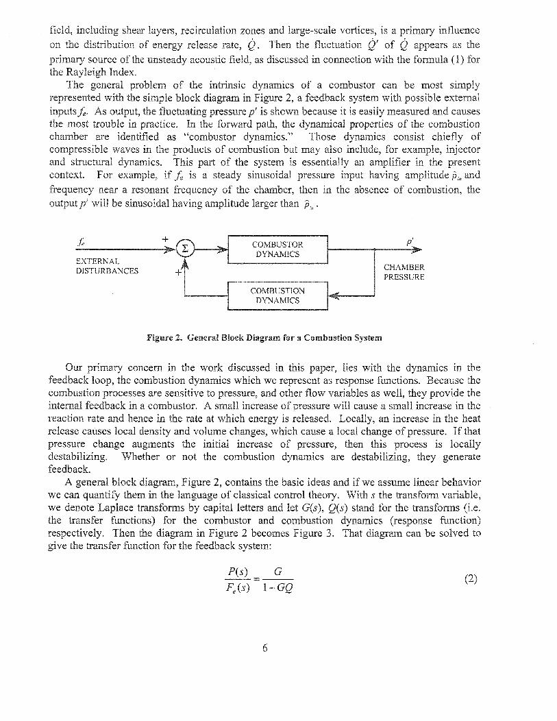
The general problem of the intrinsic dynamics of a combustor can be most simply represented with the simple block diagram in Figure 2, a feedback system with possible external inputs !e. As output, the fluctuating pressure pi is shown because it is easily measured and causes the most trouble in practice. the forward path, the dynamical properties of the combustion chamber are identified as "combustor dynamics." Those dynamics consist chiefly of compressible waves in the products of combustion but may also include, for example, injector and structural dynamics. This part of the system is essentially an amplifier in the present context. For example, if!e is a steady sinusoidal pressure input having amplitude Pin and frequency near a resonant frequency of the chamber, then in the absence of combustion, the output p' will be sinusoidal having amplitude larger than Pin'

!e + COMBUSTOR " l: '" - , DYNAMICS

EXTERNAL DISTURBANCES +,1'

COMBUSTION "'" DYNAMICS -.

Figure 2. General Block Diagram for a Combustion System

p' '" ,

CHAM BE R E PRESSUR

Our primary concern in the work discussed in this paper, lies with the dynamics in the feedback loop, the combustion dynamics which we represent as response nmctions. Because the combustion processes are sensitive to pressure, and other flow variables as well, they provide the internal feedback in a combustor. A small increase of pressure will cause a small increase in the reaction rate and hence in the rate at which energy is released. Locally, an increase in the heat release causes local density and volume changes, which cause a local change of pressure. If that pressure change augments the initial increase of pressure, then this process is locally destabilizing. Whether or not the combustion dynamics are destabilizing, they generate feedback.

A general block diagram, Figure 2, contains the basic ideas and if we assume linear behavior we can quantify them in the language of classical control theory. With s the transform variable, we denote Laplace transforms by capital letters and let G(s), Q(s) stand for the transforms (i.e. the transfer functions) for the combustor and combustion dynamics (response function) respectively. Then the diagram in Figure 2 becomes Figure 3. That diagram can be solved to give the transfer function for the feedback system:

pes) G =---

Fe(s) 1- GQ (2)

6

p

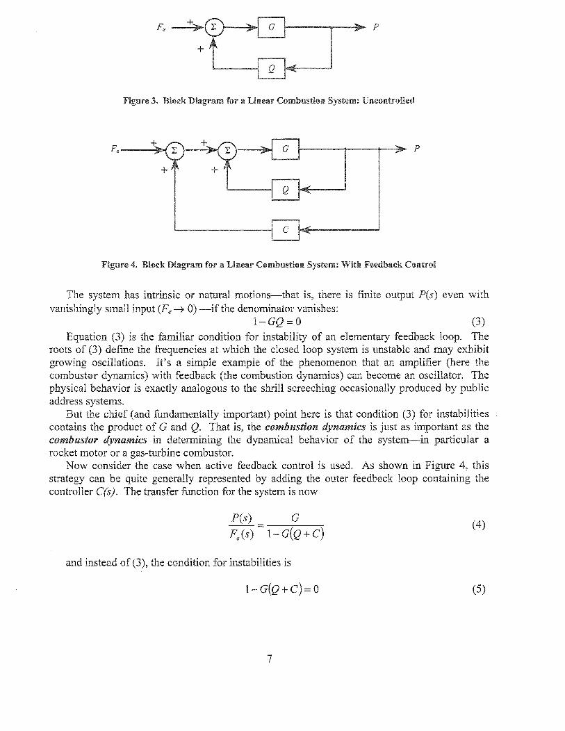
Figure 3. Block Diagram for a Linear Combustion System: Uncontrolled

p

Figure 4. Block Diagram for a Linear Combustion System: With Feedback Control

The system has intrinsic or natural motions-that is, there is finite output pes) even with vanishingly small input (Fe ~ 0) -if the denominator vanishes:

1- GQ = 0 (3) Equation (3) is the familiar condition for instability of an elementary feedback loop. The

roots of (3) define the frequencies at which the closed loop system is unstable and may exhibit growing oscillations. It's a simple example of the phenomenon that an amplifier (here the combustor dynamics) with feedback (the combustion dynamics) can become an oscillator. The physical behavior is exactly analogous to the shrill screeching occasionally produced by public address systems.

But the chief (and fundamentally important) point here is that condition (3) for instabilities contains the product of G and Q. That is, the combustion dynamics is just as important as the combustor dynamics in determining the dynamical behavior of the system-in particular a rocket motor or a gas-turbine combustor.

Now consider the case when active feedback control is used. As shown in Figure 4, this strategy can be quite generally represented by adding the outer feedback loop containing the controller C(s). The transfer function for the system is now

pes) G

Fe (s) = 1 - G(Q + C) (4)

and instead of (3), the condition for instabilities is

I-G(Q+ c)= 0 (5)

7

this context, the purpose of adding the controller is to shift the frequencies at which the natural motions (resonances or normal modes) occur; and especially to ensure that all such motions are stable. That is a problem of control design--choose the controller such that its transfer function, in combination with Q(s) and G(s), guarantees that the system has the desired behavior. Quite clearly that means that both the combustor dynamics and the combustion dynamics must be known if the design problem is to be solved satisfactorily.

In the absence of complete knowledge of the dynamics for an actual system, the problem of control becomes an ad hoc matter. That is characteristic, to some extent at least, of all existing demonstrations of active control of combustion systems, whether they are laboratory or full-scale devices. That is, based on some knowledge of the combustnr dynamics and very limited information about the combustion dynamics, a controller (and actuator) are designed and tried. Trial and error then becomes the standard strategy for improvement. central purpose of this research is to encourage replacement of and error by systematic procedures

as part of the design of combustion systems. The main point of the preceding remarks is that the combustion dynamics, and associated

response functions, are basic to the dynamics of a combustion system. Hence, methods for accurate measurement of combustion response functions are extraordinarily important for a wide range of applications.

1.2 The Connection Between the Response Function Measurements of Unsteady

Response or transfer functions must be modeled in some way to carry out analysis of the dynamical behavior of a combustion system and to do a prior design of active control. Currently, in the absence of theoretical and experimental information, simple ad hoc models are used in all applications. The main purpose of the work reported here is to develop, extend and improve methods for inferring response functions by using data obtained with laser-based diagnostics, principally PLIF and chemiluminescence. Moreover, the same methods may be used to investigate the effects of oscillation in the local generation of NO. Roughly, the strategy is the following.

The basics for the method generally is that the chemical process of producing energy is accompanied by generation of short-lived species. For combustion of hydrocarbon fuels, the radicals OH and CH are especially significant because many previous works have established that to good approximation the rate Q at which energy is released by the combustion processes locally is proportional to the concentrations of those species. How good the approximation is depends on, among other factors, the local macroscopic flow and mixing rates, and the collisional destruction of the radicals.

Hence measurement of the concentrations of OH and CH can be related to the rate of energy production. This conclusion holds true under unsteady conditions, to some approximation, if the characteristic time of the unsteadiness (here the period of impressed oscillations) is long compared to the measurement time, which in turn is short compared with the time in which the concentrations change significantly.

The method used in this work is based on impressing oscillations of pressure and measuring the fluctuations of one of the radicals in question, OH being the simplest to observe. Then by

assumption, the average and fluctuating heat release ratios (Q and Q') are proportional to the

8

average and fluctuating values of the OH concentration (denoted (OH] and [OH]' , respectively). So by assumption,

If K' have the same values,

Q =K[OH]

Q' = K'[OH]'

we can write,

Q' [OH]' -=--=~

Q [OH]

(6) a,b

(7)

A response function R p is conveniently defined as fluctuation of

value of the impressed pressure fluctuation,

heat release rate to the

0' R=..:::::.... p p'

Q'/Q or in dimensionless form R = --p p'/J3

Hence with (7), R p is expressed as a ratio of measurable quantities:

R = [OH]' /rOB] p p'/J3

(8)

(9)

where measurements give the numerator, and the denominator is obtained with pressure transducers. It is this ratio, R p' which appears explicitly in analysis of the dynamics of

combustion systems as described above.

2.0 Previous Work on Measuring Combustion Dvnamics

Three methods have been used to gain data for combustion dynamics. In order of increasingly finer spatial resolution, they are:

(i) measurement of the transfer function for a combustion region by detecting transmission and reflection of acoustic waves (e.g. Culick 2001);

(ii) chemiluminescence, measuring radiation from certain species participating in a combustion zone exposed to pressure oscillations; and

(iii) planar laser-induced fluorescence, measuring radiation induced by pulses of laser output incident on a combustion zone exposed to pressure oscillations.

Weare using both the second and third methods. In fact one unforeseen result has been to clarify the serious limitations of chemiluminescence.

Put briefly, the method based on chemiluminescence involves observation of 'natural' radiation by using either (1) a photomultiplier tube (PMT) with a slit obscuring all but a portion of the combustion zone, giving resolution in two dimensions; or (2) a CCD or similar camera capable of giving resolution in two dimensions. The great disadvantage of this method is that the radiation collected is emitted along the entire line of sight in the direction defined by the

9

orientation of the PMT or camera. Since radiation may also be absorbed, the final intensity at observation point does not in general represent only the activity of species produced in

chemical reactions. Consequently, as we have shown (Ratner or Pun? et al. 2001) seriously misleading results are often obtained. Nevertheless, the method was the first to provide results for combustion dynamics (see Table 1) and has given useful contribution to understanding combustion instabilities.

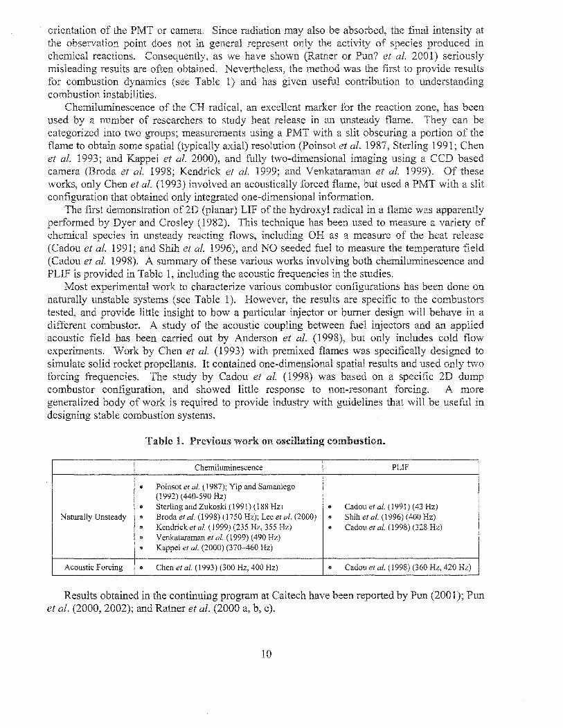
Chemiluminescence of the CH radical, an excellent marker for the reaction zone, has been used by a number of researchers to study heat release in an unsteady flame. They can be categorized into two groups; measurements using a PMT with a slit obscuring a portion of the flame to obtain some spatial (typically axial) resolution (Poinsot et al. 1987, Sterling 1991; Chen et al. 1993; and Kappei et al. 2000), and fully two-dimensional imaging using a CCD based camera (Broda et al. 1998; Kendrick et aI. 1999; and Venkataraman et al. 1999). Of these works, only Chen et al. (1993) involved an acoustically forced flame, but used a PMT with a slit configuration that obtained only integrated one-dimensional information.

The first demonstration of 2D (planar) of the hydroxyl radical in a flame was apparently performed by Dyer and Crosley 982). This technique has been used to measure a variety of chemical species unsteady reacting flows, including as a measure of the heat release (Cadou et al. 1991; and Shih et al. 1996), and NO seeded fuel to measure the temperature field (Cadou et al. 1998). A summary of these various works involving both chemiluminescence and PLIF is provided in Table 1, including the acoustic frequencies in the studies.

Most experimental work to characterize various combustor configurations has been done on naturally unstable systems (see Table 1). However, results are specific to the combustors tested, and provide little insight to how a particular injector or burner design will behave a different combustor. A study of the acoustic coupling between fuel injectors and an applied acoustic field has been carried out by Anderson et al. (1998), but only includes cold flow experiments. Work by Chen et al. (1993) with premixed flames was specifically designed to simulate solid rocket propellants. It contained one-dimensional spatial results and used only two forcing frequencies. The study by Cadou et al. (1998) was based on a specific 2D dump combustor configuration, and showed little response to non-resonant forcing. A more generalized body of work is required to provide industry with guidelines that will be useful in designing stable combustion systems.

Table 1. Previous work on oscillating combustion.

Chemiluminescence PLlF

" Po in sot et al. (1987); Yip and Samaniego (1992) (440-590 Hz)

" Sterling and Zukoski (1991)(188 Hz) " Cadou et al. (1991) (43 Hz) Naturally Unsteady .. Broda et ai. (1998) (1750 Hz); Lee et al. (2000) .. Shih et al. (1996)(400 Hz)

.. Kendrick et al. (1999) (235 Hz, 355 Hz) .. Cadou et al. (1998) (328 Hz)

.. Venkataraman et at. (1999) (490 Hz)

" Kappei et al. (2000) (370-460 Hz)

Acoustic Forcing e Chen et al. (1993) (300 Hz, 400 Hz) " Cadou et al. (1998) (360 Hz, 420 Hz)

Results obtained in the continuing program at Caltech have been reported by Pun (2001); Pun et al. (2000,2002); and Ratner et al. (2000 a, b, c).

10

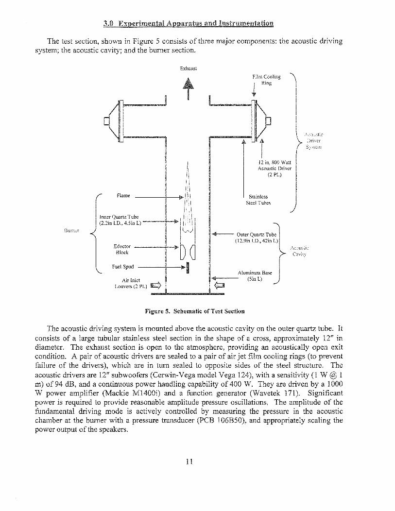
The test section, shown in Figure 5 consists of three major components: the acoustic driving system; the acoustic cavity; and the burner section.

Burner

Exhaust

Flame

Inner Quartz Tube (2.2in LD., 4.5in L) -----'jr--. I

Eductor -+--II> Ib ~ Block \J

Fuel Spud -~I Air Inlet

Louvers (2 PL)

Film Cooling

~ Ring

12 in, 800 Watt Acoustic Dri ver

(2 PL)

Stainless Steel Tubes

-<011011-- Outer Quartz Tube (12.9in l.D., 42in L)

Acoustic Driver System

ACl)LlSlic

Aluminum Base 1+--- (Sin L)

Cnvity

Figure 5. Schematic of Test Section

The acoustic driving system is mounted above the acoustic cavity on the outer quartz tube. It consists of a large tubular stainless steel section in the shape of a cross, approximately 12" in diameter. The exhaust section is open to the atmosphere, providing an acoustically open exit condition. A pair of acoustic drivers are sealed to a pair of air jet film cooling rings (to prevent failure of the drivers), which are in turn sealed to opposite sides of the steel structure. The acoustic drivers are 12" subwoofers (Cerwin-Vega model Vega 124), with a sensitivity (l W @ 1 m) of 94 dB, and a continuous power handling capability of 400 W. They are driven by a 1000 W power amplifier (Mackie M1400i) and a function generator (Wavetek 171). Significant power is required to provide reasonable amplitude pressure oscillations. The amplitude of the fundamental driving mode is actively controlled by measuring the pressure in the acoustic chamber at the burner with a pressure transducer (PCB 106B50), and appropriately scaling the power output of the speakers.

11

The acoustic cavity consists of an aluminum ring, closed at the bottom end. It has two sets of inlet louvers cut on opposing sides to allow air to flow into the tube, while providing an acoustically closed end condition. A large diameter-matched quartz tube rests in a thin register on the aluminum ring, and extends for an additional 42". Quartz was used in order to withstand high flame temperatures, as well as to allow transmission of the ultraviolet laser sheet and fluorescence signal. The tube also has several laser-drilled holes at various locations to provide instrumentation entry ports.

The burner sections are shown in Figure 6, in the two configurations used. This design allows for a variety of different flameholder configurations to be easily tested. Fuel for the burner is 50% methane premixed with 50% CO2 gas to increase the mass flow. The pre mixer inlets for each gas are choked, in order to prevent disturbances from propagating upstream and affecting flow rates.

( \ TOP

VIEW

SECTION A-A

~ " .~UEL SPUD Jt....--0.3985 1.0. H H

(a)

) I (

/

\ TOP \ VIEW

: SEcnON 8-8

CERAMIC

C:==;:::::s::. 3··:~OLDER

Jl~ , H ,

(b)

Figure 6. (a) Aerodynamically Stabilized Burner (b) Bluff-Body Stabilized Burner

Figure 7 is a diagram of the gas feed system. The mixture is subsequently passed through a laminar flow element (Meriam Model 50MJ1 0 Type 9) to measure the flow rate. It then exits the fuel spud and entrains atmospheric air into the stream. The volumetric flow rate through the spud is 2.14 SCFM, yielding ajet velocity of30 mls (Re = 20,000). Each burner quartz tube has two 1/8" slits cut on opposite sides, in order to allow the laser sheet to pass through and illuminate the flame. The slits eliminate luminescence of the quartz tube caused by the laser sheet, which was interfering with the fluorescence signal.

12

i To Burner

Impinging Sonic

Jet Premixer ""

Flow Can tro!

Regulated Pressure Indicator

/'

Bottle Pressure Indicator

/'

Figure 7. Gas Feed System

3.1 Chemiluminescence - Some Results

Two-Dimensional Flame Structure

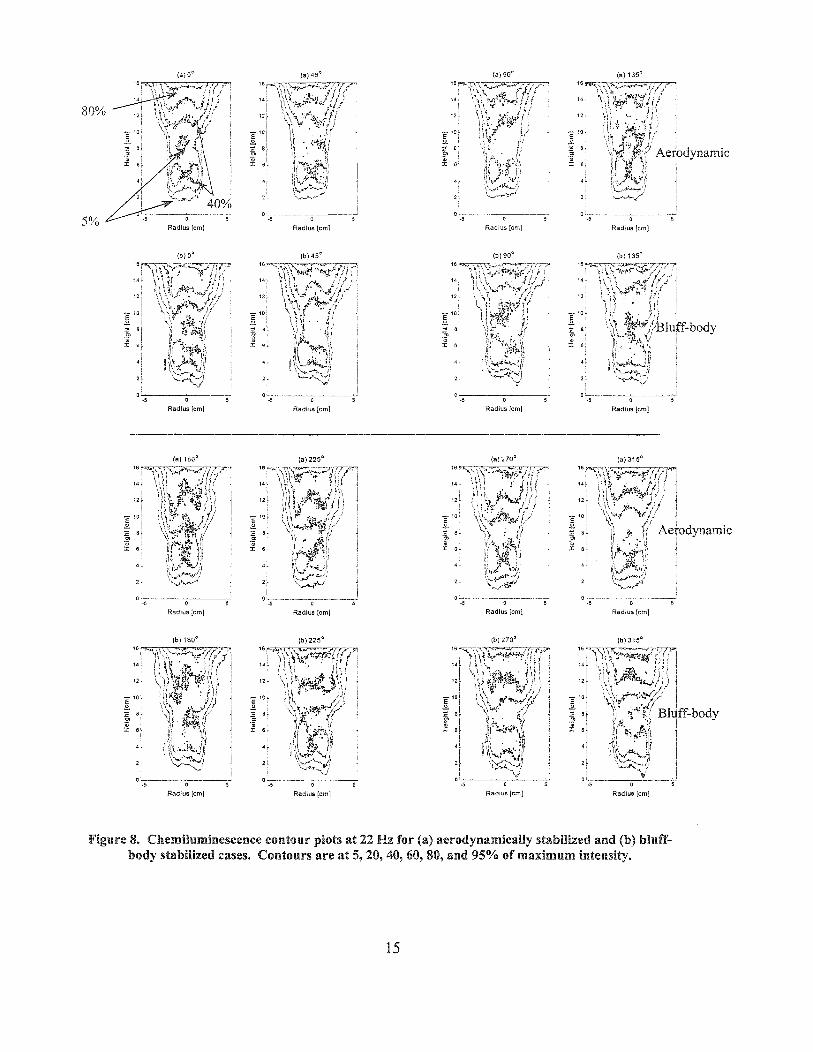
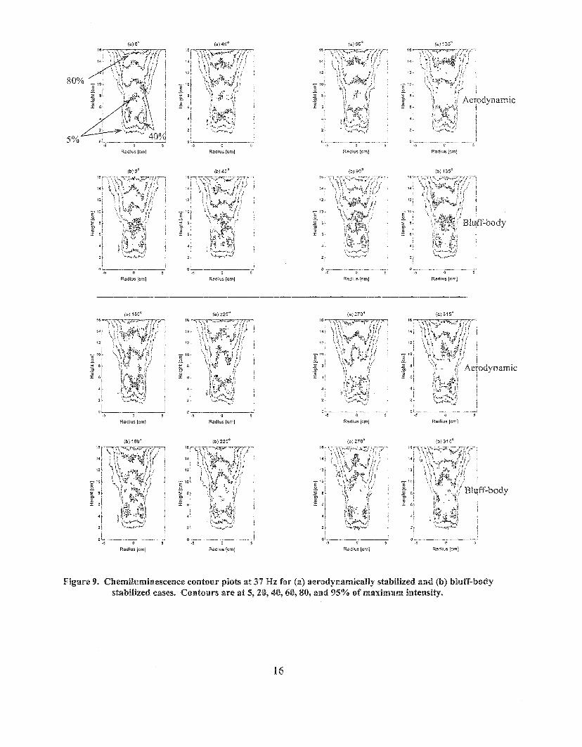
Single shot chemiluminescence images from the Phantom V 4.0 camera were smoothed using a 3x3 median filter in Matlab. Images were then averaged by phase-locking to the pressure signal. Images were selected by locating their temporal locations, and selecting the images to be averaged based on their proximity to the sixteen phase divisions used. Approximately 15 images were used on average at each phase position. The maximum phase resolution jitter was found to be less than 2 degrees in all cases. Contours were computed and plotted for each case (five forcing frequencies x two burners) showing eight phases in a cycle. Only conditions at forcing frequencies of 22 Hz and 37 Hz are displayed in Figure 8 and Figure 9. Contour levels are plotted at 5, 20, 40, 60, 80, and 95 percent levels of the maximum intensity of the 0 degree phase contour plot for each case. In all cases, the phases are taken as a sine wave, with 0 degrees corresponding to a zero crossing with a rising edge.

For forcing at 22 Hz (Figure 8), the bluff-body burner shows a larger stabilization zone than the aerodynamic burner (40% contour), centered at approximately a height of 5 cm. Note that the center "hole" at 8 ern at a phase of 0 degrees is actually at a contour of 5%, and not 40%. Characteristics to note in both cases are the traveling of a wave in the upstream direction on the outer edge of the flame, from 0 to 180 degrees. At 180 degrees, the wave reverses itself, and

13

travels back downstream. There is also a distinct change in intensity, as the flame oscillates. intensity contour at 40% can be seen to grow into tube as flame evolves

o to 180 degrees, and in the bluff-body case even connects with the 40% contour levels in the stabilization zone. As the pressure changes from 180 to 360 degrees, these intensity zones separate from each other, and travel back downstream. These two oscillating characteristics are generally observed for each forcing frequency, except for the 55 Hz case.

At a frequency of 27 much the same phenomenon is observed, with a decrease the amplitude of the outer propagating wave. In addition, there appears to be a superimposed higher frequency, lower amplitude outer wave, continuously traveling downstream. As the forcing frequency is increased to 32 Hz the intensity of the flame in the burner tube has diminished. Once the acoustic oscillations reach 37 (Figure 9), an interesting reversal occurs. The contours in the stabilization zone show a significantly larger 40% contour for the aerodynamically stabilized burner, than the bluff-body stabilized case. Recall in all previous cases, the bluff-body stabilized burner yielded stronger stabilization zones, or at least zones comparable to that of the aerodynamically stabilized burner. Finally for the 55 case (not shown here) there is essentially no change between contours at different phases. low amplitude traveling waves on outer are present, but none the oscillations of intensity, or flame shape that occurred in previous situations. Thus the response of the flame is evidently much reduced as the impressed frequency increases.

14

80%

5% o Radius [oml

i o~.'~----~O~----~5

Radius [em]

Radius [em]

(b) 180'

Radius (om]

Rad!us [em]

(b)45'

1e~~~~~,,"j)!(---': t>' • ,,:f f ~ , j

14~ ~\)' P I} r )' ~L\' ·~v)f J

12 ~ I"\' . J.i~ '1\' ~& ji \.,\(-,: .r;' 'E 1O \\[' I: "'- \' ~ , ~) ~ ~:; '1' '0 J:i~.(~--;~\\ :r:

\l~J\ i~!!' ~

Radius [em1

Radius [em!

Ib) 225'

Radius [em]

o - ___ ~ _____ _ -5 0 ,

Radius [em}

(b) 90'

16~~~~::;,.-~.v:;r71T~

\ i \r,,/;,f<».t#'1:! ' 14," '\.. *,' .. f,/"·

i\'V"'~lrI ". \ \; , , . : j/ ' , 'I "rn ./

K10"

'ill mliJj't~~ l>t .\ )

\ Q~~ 1> ~

,. -;; J: "

4,

2·

"

t:'·· . . J( ,F"'-} " ,( fit ;~~ '!'\~JI7 i 1'(:' . n "~~"~_/J

Y

o Radius [em I

(a) 270'

Radius (em}

Radius [em1

(b) 135'

16~0~~~/,/{7' j4~ ~\ .,\'~ 1!~~ (¥''j'--'

~1\\\Jftr. ",~. !;/ ". '>it '" .' ~\( . 'E10-

"'- "~~ ~~!(Bluff-body ~ ,.

'0 ~r'~""1l 'i; J: ,. il ;. ' •• ,>!:~ \\,

~I, 'ill " '\':~!;

"~1 ,. .\~.! " .I

Radius [em]

(a) 3150

Radius lem1

(b) 315'

Figure 8. Chemiluminescence contour plots at 22 Hz for (a) aerodynamically stabilized and (b) bluff­body stabilized cases. Contours are at 5,20,40,60,80, and 95% of maximum intensity.

15

5%

(b)O'

Radius {em]

(0) 180'

Radius [em}

(b) 180'

I : O~' _____ ~ ________ '

·5 0 5

Radius (emj

Radh.ls [em]

O~_5~----~O~----~~

Radius [em]

Q'~.5------~O------~~

Radius [em]

(b) 225'

Radius {em]

Q --.---------·5 0 5

Radius [em]

(b) 90'

O~_5~------O~------~

Radius {em]

(a)270'

Radius [em]

Radius [em1

12-

'E 10 .

"-~ e', .~

:r: 6-

,.

Aerodynamic

Q '---~~-'~.--~---~ ·5 Q 5

RadJus [em}

Radius {em}

Radius [em}

Radius [em}

Figure 9. Chemiluminescence contour plots at 37 Hz for (a) aerodynamically stabilized and (b) bluff-body stabilized cases. Contours are at 5, 20, 40, 60, 80, and 95% of maximum intensity.

16

3.2 Planar ..... ,''''''' .... Fluorescence of OR - Some Results

The system is based on an Nd:YAG laser (Continuum Powerlite 9010) operating at 10 pumping a tunable dye laser (Continuum ND6000), which in tum drives a mixer/doubler

system (U-oplaz) as in Figure 10. Use of Rhodamine 590 in the dye laser optimizes conversion efficiency near 564 nm, which is then doubled to approximately 282 nm to excite the (1,0) band of (Dieke and Crosswhite, 1962). Energy in excess of 30 mJ/pulse is easily provided by this system in the measurement volume. Laser energy is measured for each pulse by using a beam­splitter with an energy meter (Molectron J9LP). The detector for the fluorescence signal is an intensified CCD camera (Princeton Instruments ICCD-MAX), using a 512x512 CCD array, operated with a gate width of 200 ns. Attached to the camera is a catadioptric Fl.2 UV lens with a focal length of 10Smm. This results in a spatial resolution of 215 !lm x 215 per pixel at the focal plane. The fluorescence signal is filtered by 2 mm thick UGS and WG305 Schott glass filters. A digital delay/pulse generator (Stanford Research Systems DG-535) controlled camera

which was synchronized to the laser pulse.

ICCD camera ~ Bandpass

~ filt,,,

Sheet generating cylindrical optics

Frequency » mixer/doubler

~ Tunable dye laser

~ Nd:YAG laser

Quartz test

/

section

Burner

Figure 10. PLIF System

Data Analvsis

By taking advantage of the periodic forcing of the chamber, and assuming that the flame responds accordingly in a periodic fashion, the PLIF images can be phase-binned and averaged together, to generate the periodic response of the OR fluorescence in the flame. The oscillating pressure used to phase-resolve the images is acquired by a pressure transducer located 8 em above the fuel spud, in the zone where the flame is stabilized. Since the hydroxyl molecule is an

17

intermediary of combustion, and thus an indicator for the reaction zone in the flame, this procedure yields a proportional measurement of the heat release over a period of the acoustic driving cycle.

Due to the distributed nature of the flame under study and limitations on the ICCD camera's of view, multiple sets of images were taken at each test condition at different heights. Each

case contains a total of over 5000 images, phase-averaged into 36 equally spaced bins. Statistics indicate an even distribution among the bins, with well over 100 images per bin. The background is subtracted in each bin to eliminate scattering effects from the laser; and corrections are made for variations in spatial and shot-to-shot beam intensity. Images at the same phase but different heights are then matched geometrically, and their intensities adjusted to match in the overlap region using a least-squares minimization routine.

Some Results Combustion Response Rayleigh's

Phase-averaged images for 12 of the 36 bins are displayed in Figure 11. The relative change between images is more easily observed by noting the variation intensity over the lower right quadrant of each image. Spatial integration of the images of the OH PLIF gives the "global" concentrations at each phase angle. Representative plots of pressure and the computed heat release for the lowest driving frequency (22 Hz) are shown in Figure 12.

At driving frequencies greater than 27 Hz, the heat release contains elevated levels of higher harmonic content, which does not appear the pressure traces. This result is most clearly evident at 55 in Figure 13, which shows the ringing of higher frequency modes over the fundamental mode of heat release at this driving frequency. Again, this result is consistent for both flameholder configurations.

From the FFT of a particular condition, the frequencies of the pressure and heat release can be extracted, as well as their phase relationships. A representative plot is shown in Figure 14, displaying the relationship between the first and third modes of heat release and pressure.

The concept of a response function is well known in solid propellant combustion as a modeling tool to quantify the coupling between the pressure and the burning rate. F or solid propellants, it is typically formulated as (m' / m )/(p' / J3), where m represents the mass flux,

( )' represents fluctuation quantities, and (-) denotes time-averaged quantities (Culick, 1968). In this work, it is possible to measure a similar combustion response function directly, which can be used to close the loop between combustor dynamics and combustion dynamics (Figure 15). The combustion response function is defined as

(3)

In general, CR will be a complex quantity, since there is a phase difference between the heat release and pressure. Again, this can be evaluated globally or for spatially resolved regions, similar to the Rayleigh index, through judicious use of normalization values.

The global combustion response for both sets of burners is plotted in Figure 16. The phase of the heat release has been defined such that it lags the pressure wave. The form of the global combustion response function is similar to the classic quasi-steady response function used in

18

solid propellants (Isella, 2001), containing a single resonant peak. A simple scaling analysis of the magnitude of the fluctuations shows that for pressure amplitudes on the order of p' ~ 0.005 psi with a combustion response magnitude of 200, the heat release fluctuation is approximately 7% of the mean heat release rate.

The local combustion response is plotted in Figure 17 and Figure 18, displaying the magnitude and phase respectively. The magnitude plot (Figure 17) has been normalized using the spatial mean of the heat release rate, as opposed to a temporal mean. The plots are generated by performing an in time for each spatial extracting the fluctuating release and phase, and constructing the response function.

The spatially resolved plots of magnitude show, in general, that the bluff-body stabilized flame has a weaker response than the aerodynamically stabilized flame, which corresponds to global result (Figure 17). The phase plots (Figure 18) show regions where the heat release is in phase (0° to -90° dark red, -270° to -3600 dark blue) and out of phase (-90° to -270° orange to light blue).

Concluding Remarks

Both for reasons fundamental to the field of combustion and for understanding the behavior of combustion systems for propulsion and power generation, understanding combustion dynamics is an essential matter. For practical applications to combustion instabilities and active control, combustion dynamics appears explicitly as response or transfer functions central to the analysis of global dynamical behavior. It is impossible at the present state of the subject to compute and predict response functions. At the most basic level, the dynamical processes are always present in reacting media. Understanding those processes is intrinsically part of understanding combustion phenomena generally. Despite the growing success of numerical simulations, e.g. of turbulent combustion fields, it is still not possible to account for all fundamental processes and there is little basis for assessing the validity of the results.

Consequently there is widespread need for experimental data for the combustion dynamics of even the simplest systems. That is the motivation for developing the methods described this paper.

The results discussed here should be viewed as preliminary in the sense that improvements in the apparatus and method are still being made. In particular, the ranges of pressure and frequency to be covered will be much increased. However, we have established both the applicability of these methods to the problems of combustion instability and active control, and the four qualitative conclusions:

Chemiluminescence is useful for relatively easy application to two-dimensional flows but may give seriously misleading results for three-dimensional flows;

2) Phase-resolved PLIF gives good results for acoustically driven three-dimensional flames;

3) Both methods can successfully detect the effects of small design (geometric) changes of a burner on the dynamics of a flame;

4) Local values of the Rayleigh Index and the combustion response function can be inferred from phase-resolved PLIF measurements.

19

700 700

600 600

500 500

400 400

300 300

200 200

100 100

100 200 300 400 500 100 200 300 400 500 100 200 300 '00 500

0° 30° 60° 90°

700 700 700

600 600 600

500 500 500

400 400 400

300 300 300

200 200 200

100 100 100

100 200 300 400 500 100 200 300 400 500 100 200 300 400 500 100 200 300 400 500

120° 1500 180° 210°

700 700 700

600 600 600

500 500 500

400 400 400

300 300 300

200 200 200

100 100 100

100 200 300 400 500 100 200 300 400 500 100 200 300 400 500 100 200 300 400 500

Figure 11. OH PLIF images over a period of a sinusoidal pressure oscillation for the aerodynamically stabHized burner at 32 Hz. The intensity scale is in number of counts, and the x and y coordinates are in pixels.

20

Pressure 0.015 ----,-------,---,.-------;::::====::-:

Filtered

0.01

0.005

..(J.005

-0.01 __ -'-_______________ ..L _________ -_____ _

o 0.01 0.02 0.03 0.04 0.05 0.06 0.07 0.08 0.09 0.1 time(s)

Heat Release

1.05-

" ..} '0'" i

0.95-i

0.9~

0.85 '--_-'--_-'-______ --'-_--"---_---'-__ '--___ --1

o 0.01 0.02 0.03 0.04 0.05 0.06 0.07 0.08 0.09 0.1 time(s)

Figure 12. Pressure and Heat Release Traces at 22 Hz (aerodynamically stabilized burner).

21

Heat Release 1.05:--~----~--------:::::====~

c:

1.04

1.03 ~

1.02 i..

1.01 C'

;:!~ 1-CJ'

0.99

0.98 -

0.97 ..

0.96 ..

0.95 -~~~, .. - ... - .. -'-.. --.-------.... - .. -.--~ ... - ... ----.. -.--: o 0.005 0.01 0.015 0.02 0.025 0.03 0.035 0.04

time (5)

Figure 13. Heat Release Trace for the aerodynamicaUy stabilized burner at 55 Hz.

0.1

0.05 .. <!l "0 0

0-::;;

'" ~ -0.05 ~

-0.1 0 0.01 0.02 0.03 0.04 0.05 0.06 0.07 0.08

0.02

0.01 -<!l "0 0

0 ::;; "E '" -0.01

-0.02 0 0.01 0.02 0.03 0.04 0.05 0.06 0.07 0.08

Time (s)

Figure 14. Phase Relationships for the bluff-body stabilized burner at 27 Hz (magnitudes scaled for easy

comparison).

22

1.51---r--~--~--~===::r=::=====::;l

0.5

0

Rr -0.5

-1

-1.5

-2

-2.5 20 25 30

Driving

35 40

c·· 1st mode Bluff-body 1 st mode Aero

45 50

Frequency [Hz]

55

Figure 15. Frequency-Driven Global Rayleigh Index with and without filtering of the Mode of Pressure.

300 (!)

-g ~ 200 OJ ro

::2: 100

25 30

Combustion Response

35 40 45 50 55

Or---~-----r----~----~----r---~----~

-90

(!)

gJ -180 ---------j-----------f----------r----------~---------~--1~---3----::;::;::-~ .J:::. 0... , , , , ,

, , , I , , ) , , ,

-270 , l , , ,

---------r----------r---------T---------r---------T---------t----------360~--~----~----~--~----~----~--~

20 25 30 35 40 45 50 55 Frequency [Hz]

Figure 16. Global combustion response function

23

16

14

12

E 10 ..::. ~

J:: 8 OJ

!I)

::c 6

16

14

12

E 10 0

..--J:: 8 OJ

!I)

::c 6

4

2

22

-2.5 0-5 r [em]

27

-2.5 r [em]

-2.5 r [em]

32 37 55 Hz

o -5 -2.5 0-5 -2.5 0-5 -2.5 o r [em] r [em] r [em]

(a)

0-5 -2.5 0-5 -2.5 0-5 -2.5 0 r [em] r [em] r [em]

(b)

Figure 17. Combustion response- magnitude (a) aerodynamically stabilized (b) bluff-body stabilized.

24

16

14 50

12 100

10 1 GO

.... .s:: 8 OJ

III 200

::r:: 6

260

4

300

2

0 350

-5 -2.5 0-5 -2.5 0-5 -2.5 0-5 -2.5 0-5 -2.5 0

1 J r [em] r [em]

(a)

16

14

12

E 10 ~ .... .s:: 8 OJ

III

::r:: 6

4

2

-2.5 0-5 -2.5 0-5 -2.5 0-5 -2.5 0-5 -2.5 0 r [em] r [em] r [em] r [em 1 r [em]

(b)

Figure 18. Combustion response - phase (a) aerodynamically stabilized (b) bluff-body stabilized.

25

References

Broda, J.C., Seo, S., Santoro, RJ., Shirhattikar, and Yang, V. (1998) "An Experimental Study of Combustion Dynamics of a Premixed Swirl Injector", Twenty-Seventh Symposium (International) on Combustion, The Combustion Institute.

Chen, T.Y., Regde, U.G., Daniel, B.R., and Zinn, B.T. (1993) "Flame Radiation and Acoustic Intensity Measurements in Acoustically Excited Diffusion Flames", J. Prop. Power, Vol. 9, No.2.

Culick, F.E.C. (1968) "A Review of Calculations for Unsteady Burning of a Solid Propellant", AlA A Journal, Vol. 6, No. 12, pp. 2241-2255.

Culick, F.E.C. (1987) "A Note on Rayleigh's Criterion", Comb. Sci. and Tech., Vol. 56, pp. 159-166.

Culick, F.E.C. (1988) "Combustion Instabilities in Liquid-Fueled Propulsion Systems-An Overview," AGARD 72B Specialists' Meeting of the Propulsion and Energies Panel, AGARD CP450.

LR., Price, R.B., Sugden, T.M., and Thomas, A, (1968) "Sound Emission from Open Turbulent Premixed Flames", Proc. Roy. Soc., Vol. 303, (pp. 409---427).

{sella, G.C. (2001) "Modeling and Simulation of Combustion Chamber and Propellant Dynamics and Issues in Active Control of Combustion Instabilities", Ph.D. Thesis, California Institute of Technology, Pasadena, California.

Kendrick, D.W., (1995) "An Experimental And Numerical Investigation Into Reacting Vortex Structures Associated With Unstable Combustion", Ph.D. Thesis, California Institute of Technology, Pasadena, CA.

Lord Rayleigh, J.W.S. (1878) "The Exploration of Certain Acoustical Phenomenon," Royal Institution Proceedings, Vol. VIII, (pp. 536-542).

Lord Rayleigh, J. W .S. (1945) The Theory of Sound Vol. 11, Dover Publications, N.Y.

McManus, K., Yip, B., and Candel, S., (1995) "Emission and Laser-Induced Fluorescence Imaging Methods in Experimental Combustion", Experimental Thermal and Fluid Science, Vol. 10, (pp. 486-502).

Najm, H.N., Paul, P.R., Mueller, CJ. and Wychodd, P.S. (1998) "On the Adequacy of Certain _______ " Combustion and Flame, Vol. 113, (pp. 312-332).

Poinsot, T.J., Trouve, AC., Veynante, D.D., Candel, S.M. and Esposito, EJ. (1987) "Vortex-Driven Acoustically Coupled Combustion Instabilities," J. Fluid Mech., Vol. 177, (pp. 265-292).

Poinsot, TJ. and Veynante, D.D. (2000) "Numerical Combustion."

Pun, W. (2001) "Measurements of Thermo-Acoustic Coupling," Ph.D. Thesis, California Institute of Technology, Pasadena, CA.

Pun, W., Palm, S.L., and Culick, F.E.C. (2000) "PLIF Measurements of Combustion Dynamics in a Burner under Forced Oscillatory Conditions" AIAA-2000-3123, presented at the 36th AIAA Joint Propulsion Conference, Huntsville, AL.

Pun. W., Ratner, A and Culick, F.E.C. (2002) "Phase-Resolved Chemiluminescence of an Acoustically Forced Jet Flame at Frequencies < 60 Hz," 40'h AIAA Aerospace Sciences Meeting, AlAA 2002-1094, Reno, NV.

26

natner, A., Pun. W., Palm, S.L. and Culick, F.E.C. (2002a) "Phase-Resolved NO Planar Laser-Induced Fluorescence of a Jet flame in an Acoustic Chamber with Excitation at Frequencies < 60 " to appear in Proceedings of the Combustion Institute, Vol. 29.

Ratner, A, Palm, S.L., Pun. W., Ramirez, 8. and Culick, F.E.C. (2002b) "Flame Response to Excitation at Frequencies < 60 Hz as Measured by Phase-Resolved NO " 4dh AIM Aerospace Sciences Meeting, AIAA-2002-0195, Reno, NY.

Ratner, A, Pun. W., Palm, S.L. and Culick, F.E.C. (2002c) "Comparison of Chemiluminescence, OH PUF and NO PUF for Determination of Flame Response to Acoustic Waves."

Samiengo, J.M., Yip, 8., Poinsot, T., and Candel, S., (1993) "Low-Frequency Combustion instability Mechanisms in a Side-Dump Combustor", Combustion and Flame, Vol. 94, Iss. 4, (pp. 363-380).

Shih, W.P, Lee, J.G., and Santavicca, D.A, (1996) "Stability and Emissions Characteristics of a Lean Premixed Gas Turbine Combustor", Twenty-Sixth Symposium (International) on Combustion, The Combustion Institute.

Sterling, J.D., (1987) "Longitudinal Mode Combustion Instabilities in Air Breathing Engines", Ph.D. Thesis, California Institute of Technology, Pasadena, CA.

Zsak, T.W. (1993) "An Investigation of the Reacting Vortex Structures Associated with Combustion", Ph.D. Thesis, California Institute of Technology, Pasadena, CA.

27