Embed Size (px)
Citation preview

BRIDGE INSPECTION
AND
INTERFEROMETRY
by
JOSEPH E. KRAJEWSKI
A Thesis Submitted to the Faculty
of the
WORCESTER POLYTECHNIC INSTITUTE
in partial fulfillment of the requirements for the
Degree of Master of Science
in
Civil Engineering
May 2006
APPROVED:
Professor Leonard D. Albano, Advisor ________________________________
Professor Cosme Furlong __________________________________________
Professor Malcolm Ray ____________________________________________
Professor Frederick Hart ___________________________________________

i
ABSTRACT
With the majority of bridges in the country aging, over capacity and costly to
rehabilitate or replace, it is essential that engineers refine their inspection and
evaluation techniques. Over the past 130 years the information gathering
techniques and methods used by engineers to inspect bridges have changed little.
All of the available methods rely on one technique, visual inspection. In addition,
over the past 40 years individual bridge inspectors have gone from being
information gathers to being solely responsible for the condition rating of bridges
they inspect. The reliance on the visual abilities of a single individual to
determine the health of a particular bridge has led to inconsistent and sometimes
erroneous results. In an effort to provide bridge inspectors and engineers with
more reliable inspection and evaluation techniques, this thesis will detail the case
for development of a new inspection tool, and the assembly and use of one new
tool called Fringe Interferometry.

ii
ACKNOWLEDGMENTS
I wish to sincerely thank my advisor, Professor Leonard D. Albano, for his
encouragement, suggestions, patience and help in writing this thesis. His
willingness to let me go beyond the realm of Civil Engineer and into the far away
world of Interferometry (where few if any Civil Engineers have been) is
something I will never forget.
I would like to thank, Professor Consume Furlong for introducing me to
Interferometry. His enthusiasm for the subject matter has inspired me to
continue onward long after this thesis is finished.
I would also like to thank, Professor Malcolm Ray for is input, teachings and kind
words.
I thank the University of Illinois at Urbana-Champaign for allowing to study their
state-of-the-art imaging equipment.
I wish to thank Pilgrim Lutheran Church in Warwick, RI for allowing me to turn
their Fellowship Hall into an Interferometry Laboratory.
I especially thank my wife Karen for shouldering the responsibilities of daily life
that has allowed me to pursue this idea. It’s no fun and of little reward to
perform the mundane chores of life but without her doing those things I don’t
get to do this. So, in essence this thesis is as much hers as it is mine.
Lastly, I would like to thank my son Will, whose imagination far exceeds my own
because little children don’t limit their minds the way adults do. To Will the
impossible is possible.

iii
TABLE OF CONTENTS
LIST OF FIGURES…………………………………………………………v
ABBREVIATION…………………………………………………………..viii
GLOSSARY…………………………………………………………………x
Introduction ........................................................................................................................ 1 Start of an Idea ............................................................................................................. 1 A Crude Interferometry Example............................................................................. 1 Chapter 1 – Bridge Inspection.......................................................................................... 8 1.1 – The Ashtabula Bridge (One Night in Hell)................................................... 8 1.2 – After 1878 and Before 1970...........................................................................11 1.3 – Silver Bridge, West Virginia ...........................................................................12 1.4 – Bridge Inspector’s Training Manual (Manual 70) ......................................15 1.5 - The 1970’s ..........................................................................................................18 1.6 – The 1980’s .........................................................................................................18 1.6.1 – Mianus River Bridge, Connecticut ..................................................19 1.6.2 – Schoharie Creek Bridge, New York ...............................................23 1.6.3 – Hatchie River Bridge, Tennessee ....................................................24 1.7 - The 1990’s ..........................................................................................................26 1.7.1 – Manual 90 ............................................................................................26 1.7.2 – Fatigue and Fracture..........................................................................34 1.7.3 – PONTIS – BMS.................................................................................34 1.8 – Today..................................................................................................................35 1.8.1 – Bridge Inspection Reliability ............................................................36 1.9 – Chapter Summary ............................................................................................39 Chapter 2 – Interferometry .............................................................................................41 2.1 - Background ........................................................................................................41 2.2 - Comparison of SAR to Civil Engineering Terrain Mapping....................45 2.1 – Down to Earth Interferometry for Bridge Inspection..............................47 Chapter 3 – Field Operations .........................................................................................52 3.1 - The Required Images .......................................................................................53 3.2 – Camera ...............................................................................................................56 3.3 – Projector ............................................................................................................59 3.4 – Laptop Computer ............................................................................................60 3.5 – Laser Pointer .....................................................................................................62 3.6 – Horizontal Mounting Bar ...............................................................................62 3.7 – Support Stand ...................................................................................................63 3.8 – Tape Measure....................................................................................................63 3.9 – Mountings..........................................................................................................63

iv
3.10 – Power Source..................................................................................................63 3.11 – Field Experiments..........................................................................................64 Mock-up of a segment of a full size I-beam...............................................64 Damaged 6” Aluminum Beam .....................................................................65 Segments of Deteriorated Structural Angles..............................................66 Chapter 4 – Analysis .........................................................................................................68 4.1 – Introduction ......................................................................................................68 4.2 – Image Formatting and Noise Removal........................................................69 4.2.1 – Download Images ..............................................................................69 4.2.2 – Convert from RAW to TIFF...........................................................70 4.2.3 – Crop Images........................................................................................71 4.2.4 – Remove Noise ....................................................................................72 4.2.5 – Mask off Background........................................................................73 4.3 – Phase Calculation .............................................................................................77 4.4 – Temporal Phase Unwrapping........................................................................80 4.4.1 – Temporal Unwrapping Algorithm by Huntley and Saldner ......81 4.4.2. – Tamporal Unwrapping Algorithm by Huntley, Kaufmann and Kerr ..............................................................................................86 4.5 – Column-Wise Phase Unwrapping.................................................................88 4.5.1 – Calculate Fringe Order......................................................................88 4.5.2 – Remove 2π Discontinuities ..............................................................90 4.5.3 – Remove Fringe Pattern .....................................................................91 Conclusions ........................................................................................................................93 REFERENCES.................................................................................................................99 APPENDICES APPENDIX A – MATLAB Programs ......................................................................104 ImageProcess ............................................................................................................104 Fringe..........................................................................................................................107 Columnunwrap.........................................................................................................110 FiveFrame Subroutine.............................................................................................112

v
LIST OF FIGURES
Number Page 1. Photo of North Elevation of the Central Street Bridge ....................................... 2
2. Photo of North Spandrel Wall Damage .................................................................. 3
3. Drawing of the North Spandrel Wall Elevation .................................................... 5
4. Photo of Ashtabula Bridge......................................................................................... 9
5. Drawing depicting the night of the bridge collapse............................................... 9
6. Photo of Silver Bridge Pre-1967 .............................................................................13
7. Aerial Photo of Silver Bridge 1967 .........................................................................13
8. Eyebar chain joint where failure occurred.............................................................14
9. Typical Steel Inspection Checklist Sketch .............................................................17
10. NTSB photo of Span 20 eastbound, Mianus River Bridge................................19
11. Pin and hanger assembly...........................................................................................20
12. Photo of Schohaire Creek Bridge April 5, 1987...................................................24
13. Photo of U.S. Route 51 Bridge Collapse ...............................................................25
14. Photo of Ground Penetrating Radar System........................................................29
15. Diagram of Young’s Double Slit Experiment ......................................................42
16. Path-difference interference phenomena ..............................................................43
17. Damaged Aluminum I-beam with fringe pattern projection
demonstrating distortion of fringes .........................................................................44

vi
18. Fringe Image of deteriorated steel angle from the South End Bridge,
Agawam and Springfield, MA. ...............................................................................46
Wrapped Phase image of the same angle ..............................................................46
19. Fringe Pattern Interferometry setup.......................................................................48
20. The five π/2 shifted sinusoidal waves of the 4 fringe set...................................53
21. Interferometer Apparatus setup..............................................................................55
22. 128 Fringe Projection on paper mock-up of a 3 foot deep beam from 65
feet away at maximum projection area....................................................................59
23. PowerPoint 20 foot Target Slide on Aluminum Beam........................................60
24. Mock-up Beam, 65 feet, 0 Skew..............................................................................63
25. Mock-up Beam, 65 feet, 45 Skew............................................................................64
26. Mock-up Beam, 46 feet, 30 skew ............................................................................64
27. Aluminum Beam, 65 feet, 0 skew ...........................................................................64
28. Aluminum Beam, 10 feet, 0 skew ...........................................................................65
29. Angle Segment A .......................................................................................................65
30. Angle Segment B........................................................................................................65
31. Angle Segment C........................................................................................................66
32. Angle B, 40.5 MB TIFF Image with all 2304 rows x 3072 columns................70
33. Angle B, 2.81 MB Grayscale TIFF Image – 760 rows x 2940 columns..........71
34. No Projector Light Image (The image has been enhanced to make it visible) .. 72
35. Angle B Image with light noise subtracted out ....................................................72

vii
36. Masks of Angle B. ......................................................................................................76
Top. Initial Mask
Middle. Final Mask
Bottom. Sixteen Fringe, Phase 0 image after masking
37. Top. Ideal Wrapped Phase of 1 Fringe.................................................................78
Bottom. Angle B Wrapped Phase of 1 Fringe for row 400 of array. ..............78
38. One Fringe Phase Map at (350:500, 2720:2900) with rivet hole. ......................79
39. 256 Fringe Wrapped Map at rows 1:760 x columns 1900:2600........................81
40. Unwrapped Phase Maps .- 1, 2, 4, and 8 fringes...................................................82
41. Unwrapped Phase Map - 16 fringes ........................................................................83
42. Unwrapped Phase Maps - 32 and 64 fringes. ........................................................83
43. Unwrapped Phase Maps - 128 and 256 fringes....................................................84
44. Unwrapped Phase Difference Map - up to 2 fringes ..........................................85
45. Unwrapped Phase Difference Map - up to 8 fringes ..........................................86
46. Aluminum Beam, 4 fringe wrapped phase ...........................................................87
47. Aluminum Beam, 4 fringe order, row 250............................................................88
48. Aluminum Beam, 4 fringe with discontinuities removed ..................................89
49. Aluminum Beam, 4 fringe Estimated Phase ........................................................89
50. Aluminum Beam, Image ..........................................................................................90
51. Aluminum Beam, 4 fringe Estimated Phase ........................................................90

viii
ABBREVIATIONS
AASHO American Association of State Highway Officials.
AASHTO American Association of State Highway and Transportation Officials.
BIM Bridge Integrated Modeling
BMS Bridge Management System.
CCD Charge Coupled Device.
CIM Computer Integrated Manufacturing
DSPI Digital Speckle Pattern Interferometry.
FHWA Federal Highway Administration.
FPI Fringe Projection Interferometry.
JPEG Joint Photographic Experts Group
MHD Massachusetts Highway Department.
MRI Magnetic Resonance Imaging.
NBIS National Bridge Inspection Standards.
NDT Non-Destructive Testing.
NTSB National Transportation Safety Board.

ix
NYSTA New York State Thruway Authority.
SAR Synthetic Aperture Radar.
SLR Single Lens Reflex.
TIFF Tagged Image File Format.
TFHRC Turner-Fairbanks Highway Research Center.
USDOT United States Department of Transportation.
VI Visual Inspection.

x
GLOSSARY
Coherent Light: Light composed of only one type of light wave.
Dye Penetrant Testing: A special dye used on the surface of steel to detect
cracks. The dye is applied to the surface, will be absorbed into cracks by capillary
action, and when a developer is applied, the dye in the cracks will remain colored
while dye on the surface will turn white.
Engineering Judgment: A method of stated the structural soundness of a
structure based on observation and available information but not scientific
analysis.
Incoherent Light: Light that is composed of many different light waves.
Pachometer: A magnetic device used for locating steel reinforcing in concrete.
Phase: A characteristic of a signal that contains overall structure of the signal.
PONTIS: A Bridge Management System developed by the Federal Highway
Administration that seeks to produce more objective condition ratings of bridges
rather than subjective ratings based on the NBIS rating scale.
Primary Bridge Element: The main load carrying members of a bridge, such as
girders, deck, and piers.
Secondary Elements: The non-live load carrying members of a bridge, such as
diaphragms between girders, and lateral wind bracing.
Skew: The acute angle between the centerline of bearing support and a line
drawn perpendicular to the longitudinal centerline of a bridge structure.

xi
Rectangular bridges have a zero skew angle since the centerline of bearing and
the perpendicular line are coincident.
Skew also means the acute angle between a line drawn normal to the longitudinal
centerline of an object under study and a line drawn from a camera to the object.
Temporal Phase Shifting: Adding a known phase shift to a fringe pattern for
the purpose of calculating the phase of a set of images.
Throw Distance: The range
Unwrapping: The removal of 2π discontinuities from a wrapped phase to produce an estimate of the true phase.
Wrapped Phase: The condition where the phase is constrained between –π and +π due the trigonometric function used to calculate the phase.

1
INTRODUCTION
The Start of an Idea
Suppose there was a way of evaluating a structure’s condition without ever touching the
structure. Imagine taking this supposition and creating a system that could be utilized by
anyone with minimal training and readily available equipment. This thesis is about creating a
new bridge inspection tool that would aid in the condition rating and evaluation of bridges
with technology that is rarely used in Civil Engineering. This technology is Interferometry which
has been around for many years and its use is increasing as computer circuitry and digital
photography advance.
A Crude Interferometry Example
In 2002, the City of Fall River, Massachusetts called upon Gordon R. Archibald, Inc.
(GRA), to design the repairs for a stone arch bridge that had been damaged by fire.
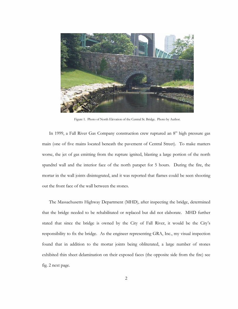
The Central Street Bridge over the Quequechan River is a spandrel filled stone arch structure
of random rubble coursing built in 1850 (see fig. 1). Central Street is located directly beneath
the Braga Bridge and is the main entrance to Battleship Cove, where the USS Massachusetts is
docked.
2
Figure 1. Photo of North Elevation of the Central St. Bridge. Photo by Author.
In 1999, a Fall River Gas Company construction crew ruptured an 8” high pressure gas
main (one of five mains located beneath the pavement of Central Street). To make matters
worse, the jet of gas emitting from the rupture ignited, blasting a large portion of the north
spandrel wall and the interior face of the north parapet for 5 hours. During the fire, the
mortar in the wall joints disintegrated, and it was reported that flames could be seen shooting
out the front face of the wall between the stones.
The Massachusetts Highway Department (MHD), after inspecting the bridge, determined
that the bridge needed to be rehabilitated or replaced but did not elaborate. MHD further
stated that since the bridge is owned by the City of Fall River, it would be the City’s
responsibility to fix the bridge. As the engineer representing GRA, Inc., my visual inspection
found that in addition to the mortar joints being obliterated, a large number of stones
exhibited thin sheet delamination on their exposed faces (the opposite side from the fire) see
fig. 2 next page.

3
Since the City of Fall River hired GRA, Inc. to design and plan the bridge repairs, we
needed to identify all the stones requiring replacement and map the limits of mortar joint
replacement so that an accurate construction cost estimate could be obtained.
The problem is that the bridge is composed of random rubble stone. That is no two
stones are dimensionally alike, and the stones are not coursed like a brick wall. Removal of any
one stone from the wall required removal of other stones above and to the sides in no
particular set pattern; in short, the spandrel walls are giant jigsaw puzzles. Using conventional
methods of measuring deterioration would require painstakingly tape measuring the location
and size of each stone required to be removed, and then the measurements would need to be
drawn on a construction plan. This exercise would be time consuming and expensive (more
expensive then the City of Fall River would be willing to pay). I decided to try something
different.
Figure 2. Photo of North Spandrel Wall Damage. Photo by Author.

4
The idea was to take a series of overlapping digital photographs of the wall, insert them
into a CAD system and trace them to create a construction plan. At the time, I had very little
knowledge of digital image processing or interferometry. However, I did understand that
digital photos could be inserted into a variety of software programs such as Word™,
Powerpoint™ and Autocad™ to name a few. In Autocad™, a photo is an object that can be
resized and distorted but cannot be edited. I knew that for the photographs to be usable, they
must be scalable, and must be taken perpendicular to the camera line of sight to minimize
distortion.
I took six photographs which covered approximately 100 linear feet of wall. In each
photograph I leaned a five foot stick against the wall as a scale. In the office the photographs
were downloaded and inserted into Autocad™. For each photograph, a CAD technician
adjusted the photos to scale, aligned the photograph to the previous photograph, traced the
stones and mortar joints, identified each damaged stone to be removed, and highlighted each
stone that needed to be removed in order to access and replace damaged stones. The process
was repeated six times and when completed, I had an elevation view with the exact limits of
removal. The entire process from taking the photos in the field to completed drawing of the
north elevation took less than 8 hours (see fig. 3 on p. 6).
This simple example demonstrates how far computers have come. The idea that data (any
data) inside a computer can flow from program to program like water was unheard of twenty
years ago. The advancement of digital photography and digital video now allows these media
to be treated like any other data in a computer; data that can be passed around, manipulated,

5
Figure 3. Portion of Repair Construction Plan. Gordon R. Archibald, Inc.
6
altered, and analyzed. Even more astounding is that anyone can, with a small amount of
training, take advantage of this technology to become more productive.
Interferometry is a subfield of optical engineering that uses image information to extract
object characteristics and solve problems. Interferometric techniques are the basis for such
diverse applications as Synthetic Aperture Radar (SAR) used in aerial reconnaissance to
Magnetic Resonance Imaging (MRI). Digital photography now makes it possible to use the
same principles found in SAR and MRI for less complex problems and with far less
sophisticated equipment.
Bridge inspection, in contrast to Interferometry, represents the low end of technology
where the methods and techniques have not changed appreciably in more than one hundred
years. Bridge inspection also fails to take advantage of the technologies that are readily
available (off the shelf technology).
The overriding theme or question to bear in mind while wading through the many pages
of this thesis is, how well can a technology created in one discipline be applied to solve
problems in another discipline.
Chapter 1 of this thesis is about the history of bridge inspection and the consequences of
no inspection. It is through this historical discourse that the arguments for and necessity of
developing new bridge inspection tools will become clear.

7
Chapter 2 starts with a brief background of interferometry. Then a comparison of modern
interferometry technology with Civil Engineering technology. Finally, the development of
interferometry for bridge inspection.
Chapter 3 discusses the first part of interferometry for bridge inspections “Field
Operations”. In addition, my test specimens will be described.
Chapter 4 is a discussion on the second part of interferometry for bridge inspection
“Analysis”. Results of analyzing my test specimens will conclude the chapter.

8
CHAPTER 1
BRIDGE INSPECTION
The current bridge inspection program instituted in the United States was created in the
late 1960’s. Its creation was in reaction to a tragedy. But it was not the first tragic failure partly
caused by poor inspection practices; it was the one that finally caused the citizenry to act.
Ninety years before, perhaps the most horrific bridge collapse in United States history
occurred.
1.1 The Ashtabula Bridge (One night in Hell)
On the evening of December 29, 1876 the Lake Shore & Michigan Southern Railway Train
No. 5, The Pacific Express was just leaving the Ashtabula Station heading westward. The train
consisted of two engines and eleven coaches. At 7:28 PM the train was crossing over the
Ashtabula River on a 150 feet long iron deck truss bridge. When, suddenly without warning,
the bridge collapsed. One engine and all eleven coaches fell eighty feet to the frozen river
below. There were 159 passengers and crew aboard, 92 were killed and 64 were injured.
Those who perished, died either in the 80 foot plunge to the ice covered river below, or were
crushed by the train engine that fell last and onto the coaches, or by fires started by the engine,
or by drowning in the river when the fires melted the ice, or by hypothermia in a blinding
snow storm after climbing out of the river and before help arrived. Forty-eight of the victims

9
were unidentifiable due to either being crushed or burned beyond recognition (their remains
were placed in 19 wooden boxes and buried in a mass grave at the Ashtabula City Cemetery).
Amazingly, 3 people walked away from this crash without injury (Whittle 1877).
The Coroner’s Jury that investigated the accident determined that the bridge had
numerous design and construction flaws; that the flaws, gradually over the eleven year life span
of the bridge caused components to noticeably weaken and sag. And if the bridge had been
carefully inspected on a regular basis by qualified personnel, the flaws would have been
discovered and the tragedy prevented.
Figure 4. Photo of Ashtabula Bridge. Note, engine Figure 5. Drawing depicting the night of the bridge shown is in the same position as the engine was the collapse. Reprinted from the Ashtabula Railway night of the collapse. Reprinted from the Ashtabula Historical Foundation web page. Historical Foundation web page.
This tragedy is said to have hastened the death of Cornelius Vanderbilt, owner of the
railroad; he died a month after the accident. It is also reported that the accident stunted the
growth of the City of Ashtabula for 30 years (in 1878 the City of Ashtabula was the same size
as the City of Cleveland) because of the negative association with the accident (the accident

10
was referred to as The Horror of Ashtabula). The Lake Shore & Michigan Southern Railway by
1900 had replaced all bridges of similar design and construction.
What did not happen was the implementation of a real system of bridge inspection. Not
long after the Ashtabula disaster, it is written that the Ohio legislature passed a bill to create
bridge standards for design, construction and inspection. The bill also called for the
appointment of an experienced engineer to oversee all bridges within the state. The bill never
became law due to fears that the appointment of the engineer would be political and that
bridge owners would relieved of any liability if the state government certified the safety of a
structure (Vose, 1887).
On a national level, there were no calls for inspection standards either. It appears that the
duel effects of influential and powerful Railroad Companies, and ignorant government officials
effectively blocked any effort for regulation. Even though in a five year span from 1873 to
1878 there were three horrific bridge failures caused by lack of inspection with Ashtabula
being the worst. The other two were the Truesdell Highway Bridge over the Rock River in
Dixon, Illinois, and the Tariffville Railroad Bridge over the Farmington River in Tariffville,
Connecticut.
The Dixon, Illinois collapse occurred on May 4, 1873 when 200 people had gathered on
the bridge to watch a mass baptism of newly converted Baptists. Approximately 56 people
were killed and 30 were wounded. The number killed is approximate since only 48 bodies
were recovered. The remaining 8 people were listed as missing and presumed dead under the
11
wreckage of the bridge in the river (the wreckage was impossible to lift out of the river with
the equipment of 1873).
The Tariffville, Connecticut collapse occurred on January 15, 1878 when a special train
carrying the attendees of a gospel revival meeting home collapsed into the Farmington River
killing 13 and injuring 70. The Western Connecticut Railroad Company, owner of the bridge,
was able to retrieve and repair the locomotives, and quickly rebuilt the bridge to the same
design. However, the cost of repairing the locomotives and rebuilding the bridge coupled with
public apprehension of the rail line, forced the company into bankruptcy on April, 1880.
1.2 After 1878 and Before 1970
After Ashtabula, Dixon and Tariffville, and before 1970, there was no national inspection
standard policy. Individual states made their own policies, if they made a policy at all.
Sometimes, for larger more complex structures, their might have been an effort to inspect
based on a loosely defined interval of every four or five years. These routine inspections
concentrated on items such as road surface condition, drainage systems, paint condition,
collision damage, and other easily identifiable conditions.
The one main structural component that was recognized as requiring a thorough
inspection on a consistent basis was the cable anchorage of suspension bridges. Failure of the
cable anchorage would collapse the bridge. The modern suspension bridge was developed in
approximately in 1840’s. By the end of the nineteenth century enough tragedies had occurred
for engineers to develop an inspection checklist of critical components. For design, the critical

12
component was adequate wind bracing, and if the bridge did not collapse soon after
construction, the critical components to inspect were the cable anchorages. In David
McCullough’s book The Great Bridge: The Epic Story of the Building of the Brooklyn Bridge he details
the early history of the suspension bridge and the sobering fact that in the mid nineteenth
century one in four suspension bridges built collapsed during or soon after construction.
For other types of structures inspection of main load carrying members were performed
during construction, when repairs were required, for planned bridge modifications, and for the
occasional failure.
Failure inspections concentrated on finding the design and construction code flaws that
led to the failure. The results of the inspection were incorporated into the codes to prevent
the same failure from happening in the future. There is little information on whether existing
structures of similar design and construction to the failed one were ever inspected or modified.
The focus was on ensuring new bridge designs avoided the same mistakes.
New bridge construction was the focus in the 1950’s and 1960’s as the interstate system
was being built across the country. After interstate construction, little money was left to
maintain or inspect bridges that had stood for years. The focus abruptly changed in 1967 with
the collapse of the Silver Bridge in Point Pleasant, West Virginia.
1.3 Silver Bridge, West Virginia
The Silver Bridge carried U.S 35 over the Ohio River between Point Pleasant, West
Virginia and Kanauga, Ohio. The bridge was an eye bar chain suspension bridge with a 700

13
foot main span and two 380 foot approach spans built in 1928. The section of U.S. 35 in the
region served as a main commercial roadway between West Virginia and Ohio operating in a
similar fashion to the interstate highways being built at the time. According to the West
Virginia Historical Society Quarterly the bridge had been inspected in 1951, 1955, 1961, and
1965 by the West Virginia Department of Transportation. Each inspection report concluded
with the statement that bridge was structurally safe (LaRose 2001). So why on December 15,
1967 at 5:00 pm, did the bridge suddenly without warning collapse, causing the deaths of 46
people?
The National Transportation Safety Board (NTSB) investigation that followed determined
that cracks in a few eye bar heads caused the collapse (Fisher 1984), that the cracks were
caused by stress corrosion, and the only available technique to detect the cracks, at the time,
would have been to take the eyebar joints apart. The NTSB Report HAR-71/01 concluded
that there was no way anyone could have foreseen the collapse. However, there were some
observations made about the inspections of the bridge.
Figure 6. Photo of Silver Bridge Pre-1967. Figure 7. Aerial Photo of Silver Bridge 1967. Courtesy of the Mason County, WV web page. Reprinted from The Charleston Daily Mail.

14
Figure 8. Eyebar chain joint were failure occurred. Reprinted from Fisher, Fatigue and Fracture in Steel Bridges (New York 1984), p. 22.
First, the bridge inspections
concentrated on roadway surface
conditions, drainage, peeling paint, and
the eyebar chain anchorages. There is
no mention of performing an in-depth
inspection of the eyebar joints.
Second, each bridge inspection concluded
with the statement that the bridge was
structurally safe but did not state how that conclusion was made. Structurally safe might have
been determined by, what until recently was acceptable, Engineering Judgment. The term
Engineering Judgment was used as a quick way, based on available information, to evaluate a
structure’s ability to carry loads safely. The available information would be inspection notes,
previous inspection reports, and observing the structure as vehicles moved across it for
excessive vibration or swaying. Engineering Judgment did not require the engineer or inspector
to backup this determination with any type of structural analysis to check capacity.
Lastly, there is no mention of whether consideration was given to the effect of increases in
live load on the bridge from the time of its construction. In 1928, when the bridge was
designed, the automobile load was 1,500 pounds and the maximum legal vehicle load was
20,000 pounds. In 1967, the average automobile weighed 4,000 pounds, the maximum vehicle
load allowed was 60,800 pounds without a special permit, and up to 70,000 pounds with a
special permit (LaRose 2001). The three fold increase in stress coupled with exposure to the

15
outside environment led to the stress corrosion and corrosion fatigue cracks which led to the
failure.
The Silver Bridge collapse highlighted the dangers of not having a comprehensive and
standardized bridge inspection system. In 1968, the United States Congress revised the
“Federal Highway Act of 1968”. The Act required the Secretary of Transportation to establish
a national bridge inspection standard and create a program to train bridge inspectors (USDOT
1995). The intent of the inspection standard and training program was to create a manual of
bridge components to inspect, what conditions could be present, and requirements to be a
bridge inspector.
1.4 Bridge Inspector’s Training Manual (Manual 70)
In the early 1970’s the National Bridge Inspection Standards (NBIS) policy, the Bridge
Inspector’s Training Manual (Manual 70), and the Recording and Coding Guide for the Structure Inventory
and Appraisal of the Nation’s Bridges (Coding Guide) were created by the Federal Highway
Administration (FHWA) to establish the procedures for biannual inspection of all bridge
structures that are part of a Federal Aid highway system; bridges on local non-Federal Aid
roads were not included. In addition, the American Association of State Highway Officials
(AASHO) published its Manual for Maintenance Inspection of Bridges (Maintenance Manual) as a
companion book to Manual 70. The NBIS policy and the Coding Guide provided
organizational structure for states to follow while Manual 70 provided the details on how to
inspect.

16
Manual 70 describes the bridge inspection process from the qualifications to be an
inspector, identifications of bridge types and components, inspection techniques for various
materials, and how to write a bridge inspection report. What is emphasized in the manual is
that the bridge inspector’s primary duty is to record the condition of the bridge as accurately as
possible but not necessarily assign a numerical condition rating. The main tool of inspection is
sight and the manual provides descriptions and photographs of the various deteriorated
conditions to record.
For superstructure inspection, guidelines were included for identifying various conditions
such as corrosion, cracking, splitting, connection slippage, deformation due to overload, and
damaged caused by collisions.
The Manual 70 says to measure the extent of the damage or deterioration. For steel
members, the manual provides a simple way to classify rust (light, moderate, severe), says to
look for buckling and kinks in members, and a method for detecting stress concentrations by
observing the cracking of paint near connections. Section 13 of Chapter 5, describes types of
steel bridges and components, stating for each one where to look for deterioration.
Throughout Section 13 the main inspection tool is visual recognition of problems. Sound is
mentioned as an inspection tool for banging of bridge components while vehicles travel across
the bridge. Feel is mentioned to measure excessive vibrations.
Overall, Manual 70 lacked sufficient information on how to measure deterioration and
deformation accurately and quickly. Deformation detection is very difficult due the overall
size of bridge members. If the deformation is large (say 25% or more of a member

17
dimension) then it is likely to been seen. But, if it is less than 25%, then the deformation will
probably not be noticed. Deformation measurement is even more difficult because one has to
find the limits of the deformation and magnitude.
Figure 9. Typical Steel Inspection Checklist Sketch. Reprinted from Manual 70, p. 5-44.
The manual’s emphasis on inspectors reporting information only and not assigning a
condition rating left states with lots of information but no way to easily rank bridges from
worst to best in order to budget their limited financial resources. Manual 70, however, was a
start and over time, the manual would be supplemented and the bridge inspection process
would evolve.

18
1.5 The 1970’s
In the seventies, the FHWA expanded the NBIS policy to include local non-Federal Aid
road bridges, defined bridges as structures with spans over 20 feet, revised the Coding Guide,
and mandated that all bridges defined by NBIS policy be inspected and inventoried by the end
of 1980. AASHO changed its name to the American Association of State Highway and
Transportation Officials (AASHTO), revised the Maintenance Manual, and developed the
Guide Specifications for Fracture Critical Non-Redundant Steel Bridge Members. Fracture Critical
Members are defined as:
Members or member components are tension members or tension components of members whose failure would be expected to result in collapse of the bridge. (AASHTO Guide Specifications for Fracture Critical Bridge Members)
Fracture critical steel members became a concern right after the collapse of the Silver
Bridge and subsequent localized fracture failures demonstrated a need for standards (Barson
1987. 526-537). Throughout the seventies Manual 70 remained the same along with visual
inspection remaining the primary tool of inspection.
1.6 The 1980’s
In the eighties, the NBIS was expanded to include culverts. A culvert is defined as A
drainage opening beneath a roadway embankment (USDOT 1995. 19-1). The FHWA added the
Culvert Inspection Manual as a supplement to Manual 70. The decade included three major
tragedies that showed the national inspection program was far from perfect.
19
1.6.1 Mianus River Bridge, Connecticut
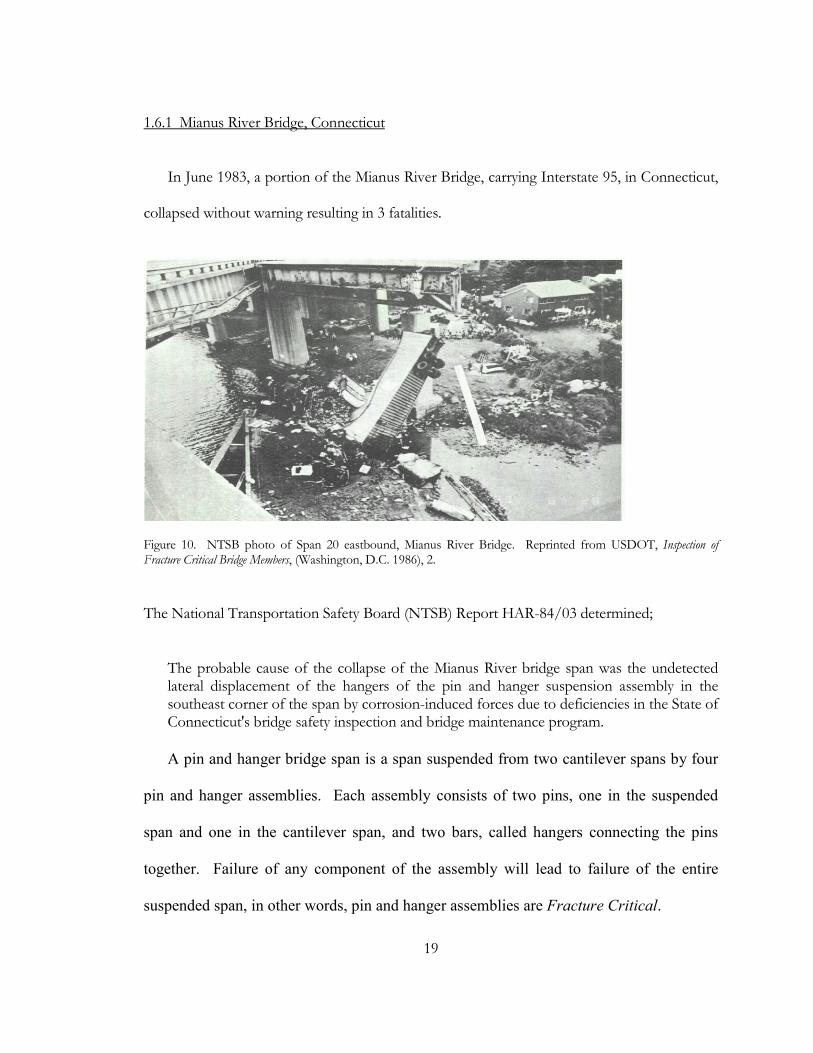
In June 1983, a portion of the Mianus River Bridge, carrying Interstate 95, in Connecticut,
collapsed without warning resulting in 3 fatalities.
Figure 10. NTSB photo of Span 20 eastbound, Mianus River Bridge. Reprinted from USDOT, Inspection of Fracture Critical Bridge Members, (Washington, D.C. 1986), 2.
The National Transportation Safety Board (NTSB) Report HAR-84/03 determined;
The probable cause of the collapse of the Mianus River bridge span was the undetected lateral displacement of the hangers of the pin and hanger suspension assembly in the southeast corner of the span by corrosion-induced forces due to deficiencies in the State of Connecticut's bridge safety inspection and bridge maintenance program.
A pin and hanger bridge span is a span suspended from two cantilever spans by four
pin and hanger assemblies. Each assembly consists of two pins, one in the suspended
span and one in the cantilever span, and two bars, called hangers connecting the pins
together. Failure of any component of the assembly will lead to failure of the entire
suspended span, in other words, pin and hanger assemblies are Fracture Critical.

20
Figure 11. Pin and hanger assembly. Reprinted from Silano, Bridge Inspection and Rehabilitation. (New York 1993), p. 194.
The deficiencies in the State of Connecticut bridge inspection program were obvious.
First, recall that in the seventies, AASHTO had written a guide specification for fracture
critical members that not only provided information on design but also maintenance.
Second, the drainage system on the bridge had been paved over. Without a drainage
system, water and road salts were allowed to flow through the bridge deck expansion
joints directly onto the pin and hanger assemblies. Third, the bridge inspectors lacked a
checklist of pin and hanger assembly conditions to look for which meant that they did not
check the alignment. Lastly, no one in the Connecticut DOT saw the connection between
the all the contributing factors that led to the failure.

21
The NTSB Report made thirty-one recommendations for improving the safety of
bridges. The recommendations were divided into Design (7), Maintenance (5), and
Inspection (19). The Inspection recommendations were subdivided into Management,
Reports, and Procedures.
Management recommendations concentrated on increasing review and oversight of
the inspection program by individual states. At the federal level, the recommendation to
the USDOT was to create a bridge inspection audit program ensure compliance of the
NBIS policy by the states.
Report recommendations consisted of improving quality and depth of the inspection
reports especially for fracture critical, large and complex structures. Specific
recommendations were;
1. List critical elements with individual condition rating and narrative
explanation.
2. List observations and measurement of alignment of members.
3. List special equipment required to perform inspection and provide reasons
why the equipment was needed.
Procedure recommendations consisted of expanding the number of bridge components
and conditions requiring inspection. Specific recommendations were;
1. States should prepare special individual inspection manuals for large or complex bridges.

22
2. States should review all available inspection manuals, guides and standards by FHWA and AASHTO, and incorporate those which are applicable into the state bridge inspection program.
3. FHWA should develop a detailed and comprehensive integrated bridge inspection procedure based on Manual 70, and the AASHTO manuals for bridge maintenance and inspection of bridges.
4. FHWA should develop a model bridge inspector’s field handbook in a checklist format. The checklist should include elements of an integrated bridge inspection procedure.
5. FHWA should develop procedures for inspection of hidden elements of pin and hanger assemblies that do not involve dismantling the assemblies.
6. FHWA should develop dimensional standards for the alignment of bridge spans to aid in detecting misalignments of pin and hanger assemblies.
7. Change the NBIS policy to require inspections and load rating of sufficient depth and detail to encompass all elements critical to structure safety.
8. Change Manual 70 to prescribe mandatory examination and inspector evaluation of critical elements as well as overall condition, and also describe an optional methodology for effective on-site inspection.
9. Produce an objective standard for repair and replacement of pin and hanger assemblies according to measured conditions of misalignment, distortion, or changes in the position of elements in the assembly.
The recommendations expanded the laundry list of bridges components and conditions
bridge inspectors would be responsible to report. In addition, bridge inspectors would now be
required to assign condition ratings to critical bridge components. Finally, the
recommendations called more accurate and precise measurement of condition problems.
In 1986, the Inspection of Fracture Critical Bridge Members Supplement was published by
FHWA. The supplement reiterated the visual inspection information found in Manual 70,
outlined the planning of fracture critical inspections, discussed fatigue and fracture failure

23
mechanisms, and provided a checklist of fracture critical components and problems to visually
inspect.
1.6.2 Schoharie Creek Bridge, New York
On the morning of April 5, 1987 Pier 3 of the New York State Thruway Bridge over the
Schoharie Creek failed causing two bridge spans to collapse which sent five vehicles into the
flooded creek 8o feet below resulting in 10 deaths. Ninety minutes later Pier 2 failed causing
additional spans to collapse. NTSB Report HAR-88/02 determined that the cause was due to
scouring of the soil beneath the spread footings of Piers 2 and 3. The NTSB determined that;
1. The New York State Thruway Authority (NYSTA) failed to maintain adequate scour countermeasures around the bridge piers and abutments.
2. NYSTA bridge inspection program was inadequate.
3. There was inadequate oversight both NYSTA and FHWA of bridge maintenance and inspection.
4. The original construction plans and specifications were ambiguous.
5. The bridge lacked structural redundancy.
Subsequent studies determined that of the 577,000 bridges in the national inventory 86%
of them are over water. In 1988, the FHWA issued a technical advisory called Scour at Bridges.
The advisory provided guidelines for evaluating scour at bridges.

24
Figure 12. Photo of Schohaire Creek Bridge April 5, 1987. Courtesy of the National Bridge Inventory Web Page.
Also in 1988, the NBIS policy was changed to require states to identify bridges that are
susceptible to scour and develop special underwater inspection procedures. The changes to
the bridge inspection program were not extensive and possibly did not go far enough to
prevent another tragedy from taking place one year later.
1.6.3 Hatchie River Bridge, Tennessee
In the evening of April 1, 1989, two pile supported column bents failed causing 3 – 85.5
foot long spans of the 4,201 foot long U.S. Route 51 Bridge over the Hatchie River to collapse.
Five vehicles fell into the flooded river below. A short time later, another column bent and
span fell on top of the five vehicles killing 8. The NTSB Report HAR-90/01 determined that
the cause was due to the failure of the Tennessee Department of Transportation to check the
northward migration of the main river channel.

25
Figure 13. Photo of U.S. Route 51 Bridge Collapse. Reprinted from The Turner Fairbanks Research Center News Letter 59.1 (1995).
The NTSB called into question the adequacy of the Tennessee Department of
Transportation (TDOT) inspection and inspection report review procedures; the adequacy
of TDOT bridge maintenance guidelines; the adequacy of TDOT over-weight vehicle permit
procedures; and the adequacy of Federal guidelines and standards for highway bridge
inspection (NTSB HAR-90/01).
Once again NTSB made a list of 20 recommendations to prevent tragedies like this one
from happening again. Eleven of the recommendations were related to bridge inspection.
The bridge inspection recommendations fell into two categories; routine inspections and
special inspections.
The routine inspection recommendations consisted of expanding the inspection checklist
to include condition evaluation of bridge elements for hydraulic conditions, side slope stability
adjacent to the bridge, and water channel conditions up and down stream of the bridge. The

26
NTSB further recommended that inspectors should also determine maintenance priorities for
each element requiring repair. The priorities levels recommended were Immediate (Critical),
Scheduled (Soon), and Planning (minor). The NTSB also recommended all bridge inspectors be
trained to evaluate scour in accordance with FHWA Technical Advisory Scour at Bridges and
other publications by FHWA and AASHTO.
The NTSB stated that if the condition of an underwater bridge element cannot be
inspected visually or by feel during routine inspections because of excessive water depth or
turbidity, then a special underwater inspection should be performed. Underwater inspections
require certified divers, special equipment such as underwater cameras, and must follow
numerous state and federal regulations. The NBIS policy was changed to require underwater
inspections on bridges with underwater elements at least every five years.
1.7 The 1990’s
1.7.1 Manual 90
In the nineties, Manual 70 was replaced by the Bridge Inspector’s Training Manual (Manual 90).
The new manual was an expanded version of the old Manual 70 that also incorporated lessons
learned from the inception of the national bridge inspection program. Manual 90 is also a
book that reminds us of the numerous bridge components and conditions a bridge inspector
must know in order to evaluate a structure. Manual 90 is approximately three times the size of
Manual 70, not including supplements for culverts, fracture critical members, scour, movable
bridges, and underwater inspection.

27
What has not changed in Manual 90 verses Manual 70 is the use of visual inspection as the
main technique for evaluating bridges. The inspection tools listed in Manual 90 verses Manual
70 are virtually the same. In addition, just like Manual 70, there is no guidance on how to
measure and detect deformations.
Manual 90 does include a chapter on advanced inspection techniques for the following
situations:
1. To supplement visual inspection findings.
2. To inspect components that cannot be inspected any other way.
3. To inspect components known to have problems or caused failures on other bridges of similar design and construction.
4. To sample a percentage of critical elements to derive an approximate overall condition.
5. For complete evaluation of fracture critical members suspected of having problems.
6. To rapidly survey the condition of a bridge deck.
7. To monitor performance under service conditions.
Table 1 lists the various techniques available, what materials they are used on, and whether
they are a destructive or non-destructive technique.
The destructive techniques are used to obtain mechanical and physical properties, to
determine the extent of deterioration. For example, samples of steel are removed from a beam
to determine its yield and tensile strength, chemical properties, and notch toughness. The test
results are used to estimate the beams capacity. An example of deterioration extent

28
determination would be obtaining samples of concrete at different depths in a concrete slab
and performing chloride-ion tests to determine the depth of road salt contamination. Since,
destructive testing requires that samples of a bridge component be obtained and destroyed
during a test, they are only performed for special inspections such as damage inspections, in-
depth inspection for the purpose of producing rehabilitation or modification plans, and for
load rating when material characteristics are unknown.
Non-destructive testing (NDT) techniques are for detecting flaws in bridge components
that can not be seen or are very hard to see. The exception is the pachometer which is a
magnetic device used for locating steel reinforcing in concrete. The pachometer does not
require extensive training and the device is small and inexpensive. Another technique that is
simple to use and inexpensive is Dye Penetrant Testing.
Dye penetrant testing consists of using a special dye on the surface of steel that will be
absorbed into cracks by capillary action and when a developer is applied the dye in the cracks
will remain colored while dye on the surface will turn white.
The remaining NTD techniques require extensive training and special equipment. The
tests are rarely performed during biannual routine inspections but for special inspections in
conjunction with destructive testing techniques.
The last point about these special inspection techniques is that they are performed only on
a small percentage of bridge components due to the amount of time required to perform them
or the costs associated with performing them. The exception would be concrete deck flaw

29
detection techniques (ground-penetrating radar and infrared thermography) that can test an
entire deck in less than a day. The detection equipment is attached to a moving vehicle and
scans a strip of the deck at time.
Figure 14. Photo of Ground Penetrating Radar System. Courtesy of Infrasense, Inc. web page.

30
Table 1. Advanced Inspection and Testing Techniques.
Source: U.S. Dept. of Transportation: Federal Highway Administration. Bridge Inspector’s Training Manual/90. (Washington, D.C.: U.S. Government Printing Office, 1995), 15-1.

31
Bridge Inspector Code of Responsibility1.
A bridge inspector code of responsibility is formally written into Manual 90. The code is
divided into five responsibilities;
1. Maintain public safety and confidence.
2. Protect the public investment.
3. Provide bridge inspection program support.
4. Provide accurate bridge records.
5. Fulfill legal responsibilities.
This list of responsibilities is far different from the loosely defined list of “typical duties of the
bridge inspector contained in Manual 70.
1. Assists in the planning and preparation of bridge inspections.
2. Inspects bridge components for deterioration.
3. Sketches bridge components.
4. Photographs various problem areas.
5. Takes technical measurements.
6. Records rotation and translation data for appropriate components.
7. Notifies supervisor of hazardous conditions.
8. Makes basic computations.
9. Maintains records of inspection results.
Maintain Public Safety and Confidence. The inspector is required to perform thorough
inspections identifying bridge conditions, preparing condition reports that identify defects, and
presenting recommendations for repairing defects. The concept is that if the inspector does
1. U.S. Department of Transportation: Federal Highway Administration. Bridge Inspector’s Training Manual (Manual 90).
Washington, DC: U.S. Government Printing Office, 1995. 5-1 – 5-3.

32
his job properly bridge problems will be identified before a failure occurs which will prevent
the public from losing confidence in the bridge system.
The concept of public safety would be further expanded in the 1990’s to include
maintaining public safety during inspection. Bridge inspectors would be required to plan and
setup more elaborate temporary traffic controls and lane closures to protect the public and
provide a safe work zone for inspection. In addition, bridge inspections on high traffic
volume roadways would be required to be performed at night, usually between the hours of
11:00 pm and 5:00 am to avoid traffic congestion.
Protect the Public Investment. The bridge inspector is responsible for identifying minor
bridge problems which can be corrected inexpensively before they become major costly
problems. In addition, the inspector must also identify minor problems that if not repaired
could lead to deterioration of other bridge components (ex. Mianus River Bridge paved over
drainage system).
Provide Bridge Inspection Program Support. Manual 90 describes this responsibility by
reminding the inspector that the NBIS policy is a federal regulation and that bridge inspection
is financed by public tax dollars, therefore, the bridge inspector is financially responsible to the
public.
Provide accurate bridge records. This area of responsibility reminds the bridge inspector
that accurate bridge records are necessary to establish and maintain a bridge history file,
identify repair requirements, and identify bridge maintenance needs. In the nineties,

33
departments of transportation are developing complex computerized database bridge
management systems. Therefore, bridge inspection reports must be accurate and complete to
ensure the credibility of the management system.
Fulfill legal responsibilities. Bridge inspection reports are legal documents. The reports
must be concise, specific, quantitative, and complete. Further, the original inspection notes
cannot be altered without approval of the inspector who wrote them. In addition, Manual 90
reminds bridge inspectors that they are required to have the qualifications listed in the NBIS
policy to conduct inspections.
In 1994, AASHTO published its revised Manual for Condition Evaluation of Bridges. In it,
AASHTO defines five types of bridge inspections: Initial, Routine, In-Depth, Damage, and
Special.
1.7.2 Fatigue and Fracture
In the 1990’s inspection of fatigue and fracture details on steel would become more
important since most of the interstate bridges built in the 1950’s and 1960’s were 30 to 4o
years old, constructed of structural steel not required to meet a material toughness standard,
and designed before fatigue stress requirements. Of most concern were “All Welded”
constructed bridges.
All welded meant that bridge connections were welded instead of bolted. The method was
meant to revolutionize the bridge construction industry. However, poor field welding

34
practices and uncontrollable environmental conditions caused localized embrittlement of the
structural steel making it more susceptible to fracture and fatigue cracks. There are many
medium to large sized bridges constructed this way and most are not modified until there is a
failure. As example of waiting for failure; in 1999 two girders out five on the Interstate 295
southbound bridge over the Blackstone River between Cumberland and Lincoln, Rhode Island
fractured almost completely. The fractures that occurred at this bridge were the same as those
that occurred in 1988 on the Providence Viaduct which carries Interstate 95 over Amtrak and
several local streets in Providence, Rhode Island. Two bridges designed and constructed the
same way and built only a few years apart.2
1.7.3 PONTIS – BMS
PONTIS is Latin for bridge, it is the name given to the Bridge Management System (BMS)
developed by the FHWA in the early 1990’s. The PONTIS was developed to more accurately
quantify the condition of bridge elements and to aid the states to use their limited funds
intelligently while maintaining public safety (MHD 1995). The FHWA intended to replace the
NBIS condition rating scale which by this time was proving to be inadequate for the growing
complexity of bridge management.
While PONTIS forces an inspector to quantify and divide their condition ratings for each
component, the condition rating choices have been reduced to 4. Thus every rating is a forced
2 The Author participated in the inspection and repair of both bridges

35
fit choice by the inspector; because of this, many states still require the NBIS condition rating
along with PONTIS.
Lastly, PONTIS is not a substitute for visual inspection but an alternative method of recording
visual inspection data.
1.8 Today
Today state departments of transportation have sophisticated bridge management system
that store and manipulate data. The systems allow DOT’s to accurately manage their resources
and aid in long term planning. Several research projects are ongoing to develop models that
will predict the future condition of bridges based on available information (Bolukbasi 2004,
Estes 2003).
In addition, AASHTO is starting to lay the ground work for developing an integrated total
bridge management system that encompasses not only inspection data, but design,
construction, and maintenance as well. All data, in this bridge life cycle system, would be
stored in a graphical electronic database.
At the 2005 AASHTO Bridge Subcommittee on Bridges and Structures meeting held at
the end of June, several task force groups either held discussions or had engineers give
presentations on the subject. In particular, Task Force 17 – Welding, where Dr. Stuart Chen
gave a presentation entitled Integrated Steel Bridge Fabrication. Dr. Chen’s presentation went
beyond fabrication and suggested a life cycle system similar to Computer Integrated
Manufacturing (CIM). Dr. Chen called this system Bridge Integrated Modeling (BIM).

36
1.8.1 Bridge Inspection Reliability3
At the heart of all current bridge management systems is the information contained in the
inspection report. If the inspection report is inaccurate, then the management system will be
unreliable.
In 2001, the FHWA commissioned a study on the accuracy and reliability of visual
inspection for bridges. The study was the first comprehensive look at bridge inspection
practices, and in particular, visual inspection (VI).
The goals of the study included:
1. Providing overall measures of accuracy and reliability of bridge Routine and In-Depth Inspections.
2. Studying the influence of several key factors that affect bridge inspections.
3. Study the variation of inspection procedures and reporting among various States.
The study consisted of a survey of bridge inspection agencies, literature review, and bridge
inspection performance trials by a selected group of inspectors from around the country.
While the survey and literature review provided background information for the study, the
bridge inspection performance trials were the main focus of the study.
The survey of bridge inspection agencies revealed that;
3U.S. Department of Transportation: Federal Highway Administration. Reliablity of Visual Inspection for Highway Bridges,
Volume I: Final Report. Washington, DC: U.S. Government Printing Office, 2001.

37
1. Professional Engineers are typically not present during inspections.
2. Vision testing for inspectors is almost non-existent.
3. Visual inspection is the most frequently used nondestructive evaluation technique.
4. Most States follow similar inspection procedures and provide the same general information in their inspection reports.
The literature search did reveal a theory on how to categorize the factors that would effect
visual inspection (Megaw, 1979). Those factors included physical and psychological
characteristics such as medical conditions, effects of stress, and behavioral fears. For the
study, physical and psychological characteristics of the selected inspectors were obtained
through questionnaires and vision tests given before, during and after each inspection.
Results of the bridge inspection performance trials
1. When asked, many inspectors did not, and may not have identified, the presence of important structural aspects of the bridge that they were inspecting. The some of the structural aspects were support conditions, skew, identification of fracture critical members. Noted findings;
• Less than 25% of the inspectors indicated the support condition.
• Less than 10% of the inspectors indicated the presence of a skew.
• Less than 50% of the inspectors verified the fracture-critical status of the test
bridges.
2. There was a significant variability in the amount of time inspectors predicted that they would need and also the actual time for inspection. Predicted times ranged from a few minutes to several hours. Actual inspection times ranged similarly.
3. Routine inspections are completed with significant variability. The variability is noted in assignment of Condition Ratings and inspection report documentation. On

38
average, 4 or 5 different Condition Ratings values were assigned to each primary element. Over half the inspectors took just 4 photographs. The amount of field notes taken varied widely.
4. 95% of Condition Ratings for primary elements will vary within 2 ratings points on average. Of these ratings will vary within one ratings point.
5. Inspectors are hesitant to assign low (less than 5) or high (greater than 7) Condition Ratings which tends to group the ratings toward the middle range of the rating scale (range 5 to 7).
6. NBIS Condition Rating system definitions may not be refined enough to allow for reliable inspection results. In addition, Condition Rating values are generally not assigned through the use of a rational approach.
7. There are numerous factors that correlate with the Routine Inspection results. Some of these factors are fear of traffic, fear of heights, vision, formal training and bridge complexity.
8. In-Depth Inspections are not likely to detect and identify the specific types of defects for which this inspection is sometimes prescribed. In one instance, 300 inspections were performed on details containing small weld cracks, only 12 reports identified them. These 12 reports were made by a total of 7 inspectors out of the group of 44 inspectors.
9. A significant proportion of the In-Depth Inspections did not reveal deficiencies beyond those that could be noted during Routine Inspections.
10. Inspectors who find small detailed defects or gross dimensional defects such as impact damage on one bridge tend to find these types of defects on other bridges. Conversely, inspectors who find few defects on one bridge tend to find few defects on other bridges.
11. Less than 50% of the bridge inspectors used any kinds of tools (hammers, tape measures, etc.).
The study report concluded by making recommendations for more inspection training,
refining the Condition Rating System, and a vision testing program.

39
1.9 Chapter Summary
In the nineteenth century;
• There are very few laws governing the design, construction and inspection of bridges.
The result was numerous collapses.
• Calls for legislation to require annual or biannual inspection went nowhere.
• Bridge inspections performed by an Engineer with a degree.
• And the most used inspection technique was visual inspection.
At the inception of the current bridge inspection system, bridge inspectors;
• Did not have to condition rate bridge elements.
• The inspectors were only responsible for gathering data through written descriptions,
sketches and photographs.
• The bridge inspection manual was only 130 pages long.
• Inspectors were given as much time as they needed to complete their work.
• Inspectors worked during the day.
• And the most used inspection technique was visual inspection.
Today,
• Bridge inspectors are solely responsible for condition rating all bridge elements.
• Most bridge inspections are performed by non-engineering degreed personnel.
• The bridge inspection manual is over 3,000 pages long not including the several
supplements manuals.
• Bridge inspectors must also condition rate elements using the PONTIS system.
• Inspections must be performed during low traffic volume periods, usually between
10:00 PM and 5:00 AM on freeways and major roadways.
• Inspectors are given limited time to perform their work.
• According to a FHWA study, Visual Inspection is consistent and inaccurate.
• And the most used inspection technique is visual inspection.

40
• Bridge Management Systems (BMS) used by departments of transportation across the
country to budget their finite resources and ensure public safety rely almost
exclusively on bridge inspection reports which rely almost exclusively on visual
inspection. How reliable can BMS be when their input data is not reliable?
What is needed to produce accurate, reliable and verifiable inspection reports is to have a
group of people come to a consensus on condition ratings rather than a single person with
limited time and tools. While it is not practical to have each individual in a group personally
inspect a given bridge, it is practical to have an individual from a group collect inspection data
for a given bridge. In other words, redefine the role of the bridge inspector to be the primary
data collector, as in the early days of the NBIS, and a group member for condition rating.
Data collection should consist of photographs, sketches, written descriptions, and
measurements of structure geometry, damage and deterioration. Measurement data is the
most time consuming, difficult and important information to obtain. New methods to obtain
measurements should be explored and put into use. One of those methods is interferometry.

41
CHAPTER 2
INTERFEROMETRY
The basic definition of the word Interferometry is:
A device that uses the interference of waves (as of light) for making precise measurements. (The Merriam-Webster Dictionary (1998), s.v. “Interferometer.” )
2.1 Background
The study of the interference of light waves can be traced back to 1801 with the
experiments performed by Thomas Young in England. Young’s Double Slit experiment
demonstrated how two identical light waves interact. The experiment consisted of three
screens. The first screen (Screen A) had a single hole in it. The purpose of the hole was to
provide for a single source of light to the experiment. The second screen (Screen B) had two
slits in it set a distance “d” apart. The two slits split the light source coming from Screen A
into two light sources. The last screen (Screen C) had no holes in it. The purpose of Screen C
was for observing how the two light waves coming through Screen B interacted with each
other and the surface of Screen C.

42
Figure 15. Diagram of Young’s Double Slit Experiment.
The interaction of the light waves on Screen C produced white and black bands. Young
determined that the color of a bands is based on whether the two waves at a particular point
on Screen C are mutually destructive (dark band) or mutually additive (white band). Opposite
waves cancel each other out, and similar waves are additive.
Young was also able to determine the mathematical relationship between light wavelength
(λ), path lengths (r1 and r2), path difference (∆φ), distance between light sources (d), and sight
angle (θ ).
2.1) θπλφ
sin2
)(∆=d Ghiglia and Pritt (1998)
Screen A Screen B Screen C
Light Source

43
r2
dΘ
∆φ
O
S2
S1 r1P
CBA
LIGHT SOURCE
Figure 16. Path-difference interference phenomena. Ghiglia and Pritt (1998).
The most important aspect of this relationship is, that when θ is small, the white and dark
bands (fringes) are uniform and straight as long as the screen is flat. As long as the screen is
flat the relationship of any point to any other point on the screen can be described by a linear
function.
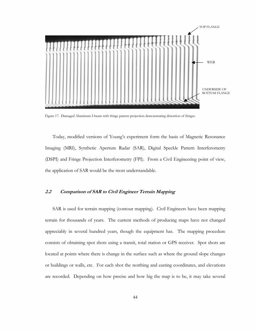
However, if the screen is no longer flat then the fringe lines will distort as a consequence
of that unevenness. With uneven surfaces the relationship between points on the screen
becomes non-linear. The interference between the light waves now occurs on differing levels
that are parallel to the screen. Think of the differing levels of interaction as elevations on a
contour map which is what interferometry is (contouring a surface). This phenomena of
optical engineering has been used and is still used in quality control of high precision
manufacturing of items such as optical mirrors and turbine blades (Ghiglia and Pritt 1998, 12).
44
Figure 17. Damaged Aluminum I-beam with fringe pattern projection demonstrating distortion of fringes.
Today, modified versions of Young’s experiment form the basis of Magnetic Resonance
Imaging (MRI), Synthetic Aperture Radar (SAR), Digital Speckle Pattern Interferometry
(DSPI) and Fringe Projection Interferometry (FPI). From a Civil Engineering point of view,
the application of SAR would be the most understandable.
2.2 Comparison of SAR to Civil Engineer Terrain Mapping
SAR is used for terrain mapping (contour mapping). Civil Engineers have been mapping
terrain for thousands of years. The current methods of producing maps have not changed
appreciably in several hundred years, though the equipment has. The mapping procedure
consists of obtaining spot shots using a transit, total station or GPS receiver. Spot shots are
located at points where there is change in the surface such as where the ground slope changes
or buildings or walls, etc. For each shot the northing and easting coordinates, and elevations
are recorded. Depending on how precise and how big the map is to be, it may take several
TOP FLANGE
UNDERSIDE OF BOTTOM FLANGE
WEB

45
hundred to several thousand spot shots to complete the map. The shot information is brought
back to the office where it is entered into a computer for processing. The computer programs
produce the elevation contours by interpolation between shot points. The computer programs
are not perfect and hand editing through a CAD program is necessary to correct errors. It
should be noted that less than twenty-five years ago (and sometimes for very small projects
today) the entire contouring process was performed by hand with pencil and paper.
In SAR terrain mapping the ground becomes the screen and two satellites emitting radar
waves replace the slits and light waves. Interference fringes appear based on the same
principles as Young’s experiments. For every point on the ground it is possible to calculate a
north and easting coordinates, and elevation. The coordinates are derived primarily from the
geometrical relationships between the satellites and the ground. The elevation at each point is
calculated using radar wavelength ( λ ), ground reflectivity (ai) distance from a satellite to the
ground (r), and a phase term. The phase is defined as the round trip the radar wave makes
from satellite to the ground and back. The formula to calculate the complete roundtrip from a
satellite to ground and back is;
(2.2)
≅
λπ ),(4
exp),(),(yxRj
yxayxg iii
The interference between the radar waves of both satellites can be calculated to produce;
(2.3) [ ]* 2
1 1 22
4( , ) ( , ) ( , ) exp ( , ) ( , )g x y g x y a x y j R x y R x y
πλ
≅ −

46
Either the real or the imaginary part produces a fringe pattern and a portion of Equation 2.3
[ ]1 2
4( , ) ( , )R x y R x y
πλ
−
represents the Wrapped Phase .
The Phase or Phase Spectra of an image contains the overall structure and characteristics
of the image. The other spectra is called the Magnitude or Intensity Spectra and as the name
implies, contains the magnitudes of the image.
A Wrapped Phase is when all the values are contained between +π and –π, as a
consequence of calculating phase with trigonometric functions. In addition, the Wrapped
Phase has 2π discontinuities, that is locations where the phase jumps from +π to –π (the
discontinuities correspond to the locations of boundaries between light and dark fringes).
In order to calculate the elevation of each ground point, the wrapped phase must be
Unwrapped. Phase Unwrapping is the removal of all the 2π discontinuities. What remains
after the discontinuities are removed is an elevation map in phase values. The last step in
calculating elevation is to create a relationship between phase value and elevation.
(a) (b)
Figure 18. (a) Fringe Image of a deteriorated steel angle from the South End Bridge, Agawam and Springfield, MA. (b) Wrapped Phase image of the same angle.

47
Without going into a deeper explanation of SAR terrain mapping, let us conclude this
comparison between mapping techniques with some important points.
1. Survey mapping relies on interpolation of elevation between a limited set of points.
2. SAR mapping relies on complex technology to interpret elevations for a large set of points that are adjacent to each other in two dimensions.
3. What we are doing with either technique is to map a surface of an object (in this case the earth). Visual inspection of bridge components is also a study of the surface of an object. So how can something like SAR mapping be adapted for the inspection of bridges.
2.3 Down to Earth Interferometry for Bridge Inspection
It would be ridiculous to assume SAR terrain mapping could be used for bridge inspection,
mostly in terms of cost. However, there are simpler, lower cost and easier methods.
One technique that could be used is Temporal Phase Shifting using Fringe Projection with
an Incoherent Light Source. Temporal Phase Shifting consists of adding a known phase shift
to a fringe pattern for the purpose of calculating the phase of a set of images. Incoherent light
is composed of many different lights waves (natural light, headlights, etc.). A coherent light
source is composed of only one type of light wave (lasers, radar, etc.).
The technique consists of projecting a series of fringe patterns from a single light
source instead of using two interfering light sources. The general procedure for FPI consists
of;
1) The fringe patterns are projected on the object in question.

48
2) For each fringe pattern a set of images is recorded.
3) Measure distances from equipment to the object (record the geometry of equipment setup).
4) The images of each fringe set are used to calculate a wrapped phase map for that set.
5) The wrapped phase maps are unwrapped and combined to produce a surface map in pixels for length and width and phase units for height, and (6) transforming the surface map into a map in real units (feet, inches, etc.).
The SAR system uses two satellites separated by a distance ‘d’, FPI similarly uses a distance
‘d’ between the projector and the camera. Also, distance from the projector and camera to the
object are ‘Rp’ and ‘Rc’ respectively. In addition, other measurements such as the distances
from the projector to the ends of the object will be helpful in the transformation of the surface
map to real units. Other than how the fringes are produced and recorded, the remaining tasks
for SAR and FPI are virtually the same. There numerous methods and techniques that can be
applied to both and which method is used is dependant upon the amount and quality of data
obtained.
Figure 19. Fringe Pattern Interferometry setup.

49
Notice that the five tasks listed for FPI can be divided into two distinct operations; (a)
Field Operations, and (b) Office Operations.
a. Field Operations
1. Fringe Projection.
2. Record Fringe Images.
3. Record Distances.
b. Office Operations
4. Calculate Wrapped Phase Map.
5. Calculate Unwrapped Phase Map.
6. Transform Map.
This separation of tasks into one of data collection and one of analysis is the same as that
of Intersection Capacity Analysis in Traffic Engineering.
The field work of an intersection capacity analysis consists of sending personnel out to the
intersection to count vehicles, record turning movements and maybe distinguish between cars
and trucks. When the personnel return from the field with the data, the traffic engineer
performs the analysis. Further, the traffic engineer is likely to discuss the data and analyses
with other traffic engineers who can verify the analysis or perform there own analysis. Finally,
additional traffic counts can taken at anytime in the future and accurately compared to
previous counts since the data is consistent and reliable. What traffic engineering has is a
reliable and consistent stream of information obtained by minimally trained personnel and that
same raw data can be analyzed and compared by any number of specialists to produce highly

50
competent results. Traffic engineering is the exact opposite of bridge inspection and
evaluation.
In deciding that FPI is worth developing as a bridge inspection tool, I wrote down numerous
questions that I hope to find answers for:
1. Cost. With hundreds of bridge inspection crews and hundreds of thousands of bridges across the country, inspection equipment must be affordable to be readily used.
2. Training. Inspection equipment should not require extensive training over and above that already provided for by basic bridge inspection training.
3. Durability. Bridges are situated in harsh environments. Any equipment used will also be subjected to the same conditions.
4. Sensitivity to the environment. Equipment measurement should be as minimally effected as possible by vibration, wind, light, temperature, humidity, etc.
5. Accuracy. How accurate is the equipment?
6. Scaling. The equipment proposed here is based on laboratory sized equipment, used on objects at a relatively close range (10 feet or less). To be used in bridge inspection will require short (<10 feet) to long range (70 feet) capabilities. There are two ways to possible paths to examining scaling; 1. scale-up the quality of the equipment or 2. use the same equipment and determine its limitations. For my thesis I have chosen to pursue path 2 in the interest of finding the limitations of the lowest cost equipment.
7. Artificial Fringes. It is assumed that the mathematical fringes projected are perfect representations of interfering light waves. Therefore, they should produce similar results.
In the next chapter the Field Operations (Data Collection) tasks will be explained by
describing the construction and experimental use of an FPI apparatus.

51
CHAPTER 3
FIELD OPERATIONS
The goal of the field operations is obtain fringe projection images and collect geometric
data that can be used for an interferometric analysis.
3.1 The Required Images
The number of images required depends on the interferometry method selected, for my
setup the number of images necessary is 47.
Image 1 - No light picture. The purpose of this image is to obtain the background light
noise so that it can be removed from each of the fringe images. The background light noise
consists of the random light waves present at the site and in every picture but is not part of the
fringe projector light source.
Image 2 - Light picture with no fringe. This image will be used to produce a mask that
will remove the background from each fringe image. The mask is a picture containing only
two colors – black and white or in mathematical terms 0 and 1. Areas in the fringe images we
want to keep are assigned a ‘1’ and areas we do not want to keep are assigned a ‘0’.

52
Images 3 through 47 - fringe images. Depending on which phase algorithm and the
quality of the equipment used, the number images required will vary. For my experiments, I
have selected the Schwider Five-Frame Algorithm (Rastogi 2001) and a maximum of 256
fringes. This algorithm is one of many Phase Shift methods for the calculation of phase. I
selected a phase shift method since it is the easiest for those with no experience in signal
processing to understand. The sacrifice for ease of use is volume of data required verses more
efficient and complex methods.
As the name implies, 5 images (frames) for each fringe are necessary to calculate the phase.
The fringes themselves are sinusoidal waves of gray scale light as seen from above. The
difference between the images in a set is that the fringe wave is shifted π/2 between images.
What we end up with is images named 0, π/2, π, 3π/2 and 2π for each fringe set.
0
π/2
π
3π/2

53
2π
Figure 20. The five π/2 shifted sinusoidal waves of the 4 fringe set.
The formula for creating the sinusoidal waves is given by;
(3.1)
cycleforcolumnsofnumbern
ntojtoiwhere
ij
njiI
1
,1,402
12
)1(2
cos
),(
=
==
+
+−
=
ππ
The increasing modulation of the fringe sets is by powers of 2 starting with 20 = 1 and
ending with 28 = 256. The fringe sets are 1, 2, 4, 8, 16, 32, 64, 128, and 256.
The purpose of phase shifting and increasing modulation by known values is to provide a
known carrier wave that goes out from the projector alone but returns to the camera with the
unknown phase of the surface of our objects.
The typical equipment used in FPI consists of a camera for recording images, a projector
for fringe projection, and a lap top computer for control and storage. There are numerous
articles describing fringe projection equipment (Buron 2005; Sansoni 2003; Sitnik, 2002 &
2004).

54
The systems described in these articles are meant for laboratory and inside use. They were
not necessarily constructed to be used in an outside environment. The equipment described in
the articles is placed in close proximity (10 feet or less) to the objects of study.
For bridges, the distance between the equipment and a typical highway bridge can range
from less than 10 feet (for close up shots) to over 70 feet (for large areas or difficult access
locations). In addition, the size of a bridge component is significantly larger than the objects
analyzed in the articles. Lastly, as the distance from the projector grows so does the area
covered by each projector pixel. What we have here is a significant scaling upwards of
distance, object size and pixel size.
After reviewing the equipment setups described in various articles and developing a list of
bridge inspection requirements and data acquisition needs. I assembled an Interferometor
apparatus with the inclusion some additional items suited for bridge inspection.
1. Camera - Cannon PowerShot S70
2. Projector - Mitsubishi LVP-SD10U
3. Computer - Toshiba Satellite M35X
4. Laser Pointer - HotShot Laser Level
5. Horizontal Mounting Bar - 72” Long Steel Level
6. Support Stand - Adjustable Steel Saw Horse
7. Tape Measure - FatMax Laser Distance Measurer
8. Mountings - Manfrotto 3D Heads and Super Clamps
9. Power Source - Direct AC, DC to AC Inverter, Generator

55
Figure 21. Interferometor Apparatus setup.
3.2 Camera.
The Cannon Power Shot S70 is a 7.1 megapixel CCD (Charge Coupled Device) with 3.6x
high quality wide angle optical zoom lens. The camera is capable of 15x optical zooming as
well. In addition, it is possible to attach higher quality lenses with the use of an optional
adapter. This camera is a mid to slightly upper range camera in terms of price and ability, but
it is a camera that bridge inspectors would have available or could obtain easily. Higher end
cameras, in particular, Digital SLRs (Single Lens Reflex) cameras would provide the greatest
flexibility and resolution (10 megapixels and up). With lower end cameras there is a sacrifice of
quality.
MOUNTING
CAMERA LASER POINTER PROJECTOR
COMPUTER
STORAGE BOX
MOUNTING BAR
STAND

56
As the resolution of the camera goes down so does the maximum number of fringes
possible. Typically, a -π to +π phase range must be defined by at least 10 pixels to be useful.
For my camera with a 7.1 megabit resolution composed of 2304 pixel rows by 3072 pixel
columns with the fringe pattern oriented vertically and running horizontally across the
columns, each –π to + π range is defined by 12 pixels (3072/256). Interestingly, if the fringes
were oriented horizontally 9 pixels (2304/256) would define the range.
Other camera considerations are control, power and storage. A camera for
interferometry must at the very least be controllable electronically through a computer or
remote control. Physically pressing the shutter button or using a mechanical remote will cause
the camera to move while taking pictures and with 47 pictures to take the potential for
mistakes is significant. The ideal method of camera control is through a computer. I control
my camera with an inexpensive downloadable program called PSRemote. With this program I
can adjust all the camera settings, take preview shots, and program a timed number of pictures
to take.
The camera is powered through an AC adapter kit. I did attempt to use battery packs
several times but the packs wore down before I could properly adjust the camera settings and
take all 47 pictures.
Picture storage is determined by several factors. First, the format used to store the
pictures. The format choices are JPEG (Joint Photographic Experts Group), TIFF (Tagged
Image File Format), and RAW. The JPEG and TIFF formats are standard formats that
compress and change RAW formatted data. The storage size of JPEG pictures can range

57
from approximately 50 kb to several megabytes. The storage size of TIFF pictures can range
up to 40 megabytes. With the standard formats there is a loss of quality in the data as camera
information is mathematically manipulated. In the RAW format, data is stored uncompressed
and unaltered and, is the highest quality data. The storage size of RAW data is 7.1 megabytes
(2304 x 3072). The problem with the RAW format is that its structure varies from
manufacturer to manufacturer and can not be read by many programs. In spite, of its
problems I elected to store pictures in the RAW format in order to preserve the unaltered data
from the camera. At the start of the interferometry analysis I compress the files into the TIFF
format.
Second, storage also has to do with where the pictures are stored. If the pictures are to be
stored in RAW format directly to the computer, via a USB cable from the camera to the
computer after every shot, the time interval between shots would be approximately 35
seconds. This means that it would take approximately 27.5 minutes to take all 47 shots. This
time period appears to be too large a time interval for interferometry. However, if the pictures
are stored in the RAW format on the camera’s memory card after every shot, the time interval
between shots would be 8 seconds. The total time to take all 47 shots reduces to 6 minutes 16
seconds. Therefore, for my experiments, pictures are stored in the camera’s memory card and
transferred to the computer later. Since all the pictures are stored on the memory card, the
card becomes the most valuable piece of equipment in the field (without the card the work is
wasted). Therefore, high quality durable cards with plenty of storage capacity should be
selected. The cards I have are Extreme III 2.0 GB Compact Flash from SanDisk. The cards
are designed for extreme weather conditions, temperatures from -13ºF to 185ºF, and are shock

58
and vibration resistant. The cards even come with a recover program just in case the card
becomes unreadable. The cards also have 20 MB/sec read and write capability.
3.3 Projector
The Mitsubishi LVP-SD10U is a lightweight (5.5 lbs.), adjustable, long range portable
projector. The image resolution is a maximum 1280 x 1024 pixels with a maximum movie
projection range (throw distance) of 40 feet. Since we are only interested in projecting fringes,
I have determined through trial and error that the projector can throw fringe patterns up to 70
feet. The size of the projection will vary with distance and the amount of zooming. For
instance, at 70 feet, the projection can be as small as 13.7 feet x 13.7 feet to as big as 26.6 feet x
26.6 feet. This means that at maximum resolution the pixel size will range from 0.12 inches x
0.15 inches to 0.25 inches x 0.31 inches. To produce the most accurate results the smallest
projection area at any distance should be used. The following is a list of the smallest
projection size and smallest pixel size for each distance;
Distance (ft.) Projection Area (ft. x ft.) Pixel Size (in. x in.)
10 2.75 x 2.75 0.03 x 0.03
20 3.33 x 3.33 0.03 x 0.04
30 5 x 5 0.05 x 0.06
40 6.83 x 6.83 0.06 x 0.08
50 8.5 x 8.5 0.08 x 0.10
60 10.2 x 10.2 0.10 x 0.12
70 13.17 x 13.17 0.12 x 0.15

59
Figure 22. 128 Fringe Projection on paper mock-up of a 3 feet beam from 65 feet away at maximum projection area.
The projector adjustments include brightness, contrast, sharpness and keystone (keystone
is a horizontal distortion of the projected image either at the top or bottom). This projector is
a slightly upper range portable projector in terms of price and ability. It is a projector that
takes little training to operate. Higher end projectors tend to either have greater resolution or
greater throw distance but not both. Lower end projectors suffer from either lack of throw
distance or resolution or sometimes both.
3.4 Laptop Computer
The Toshiba Satellite M35X lap top is a typical computer readily available today. This
computer runs on the Windows XP Professional operating system. The minimal components
the computer requires are a USB port for the camera hookup, a port (USB or Serial) for the
projector hookup, an AC power cord, the Microsoft PowerPoint program, and the PSRemote
program.

60
PowerPoint is used to project a timed slide show through the projector. The first slide is
a target slide for aiming the projector, the next slide is completely dark for taking the
background light image, the next slide is completely white for creating a mask, and the
remaining slides are the fringe projections. The first two slides are not timed slides, rather they
need a key to be pressed to advance to the next slide. This was done to aid in coordinating
PowerPoint and the PSRemote program. The remainder of the fringe projection slides
advance every 8 seconds.
Figure 23. PowerPoint 20 foot Target Slide on Aluminum Beam.
Given that the projector only projects square images and that at greater and greater
distance the height of that projection becomes far higher than is necessary. I have created
several sets of slides with varying heights of slides based on projection distance. The slide sets
are for 10 feet, 20 feet, and 70 feet. The main purpose for cropping the slides is to minimize
the distraction it might cause if it projected on a real bridge.
The PSRemote program is to adjust and control the camera, and time the taking of the
pictures. PSRemote is set to take 50 pictures at 8 second intervals to correspond to the
PowerPoint Slide Show. The extra shots for the camera timer is to aid in coordinating
PSRemote and PowerPoint.
61
3.5 Laser Pointer
The laser pointer is used as a means of providing a common centering target for the
projector and camera. The pointer is mounted midway between the camera and projector. In
addition, the pointer can be used to relate the taking of overlapping sets of pictures. For
example, two sets of images can be coordinated by taking the first set of images, then turning
the laser a known angle, retargeting the camera and projector to the new laser location, and
taking the second set of images. The technique is the same as producing a panoramic picture
from a set of pictures.
3.6 Horizontal Mounting Bar
The 72” long aluminum level for mounting the camera, laser pointer and projector
provides some advantages and disadvantages.
The advantages are its lightweight, its anodized finish will not corrode easily, the I-beam shape
allows for easy clamping of mountings and clamping to the support legs, and since it’s a level
the equipment can be easily leveled.
The disadvantage is that it is susceptible to torsion particularly where the projector is mounted
(the projector weighs 5.5 lbs). Targeting the camera or projector is difficult. In addition, on a
recent attempt to setup the equipment at a bridge in Pawtucket, RI, the wind caused torsional
vibration at the projector.

62
3.7 Support Stand
The heavy gauge steel saw horse with adjustable legs was selected to provide very stable
stand that can withstand wind loading. A transit tripod stand for supporting the 72” long
mounting bar proved to be too precarious and unstable. Using two tripods might be an
alternative to the steel saw horse.
3.8 Tape Measure
The FatMax Laser Distance Measurer by Stanley Tools can readily measure distances to
100 feet with an accuracy of 1/8”. The purpose of the laser measurer to measure the distances
from the camera, laser pointer, and projector to the ends and center of the object under study.
This geometric information is necessary to transform the phase map into real world
measurements. There are more expensive laser type devices with higher precision available. In
addition, the geometric relationship between the equipment and the object can be obtained
using surveying equipment.
3.9 Mountings
The mountings for the equipment provide multi-directional adjustment and have
graduated tick marks for tracking horizontal angle adjustments.

63
3.10 Power Source
As mentioned previously, the camera and computer will not operate for a long enough
period of time on battery power to complete taking all the required pictures. An AC power
source is necessary to run the projector, camera and computer. The total power required is
460 watts minimum, therefore any type of AC source can be used. I have tried using a 750
watt inverter connected to a stand alone 12 volt small ATV (All Terrain Vehicle) battery and a
car engine battery with success.
3.11 Field Experiments
With the apparatus described above, I have experimented with a variety of structural shapes at
various distances and skew angles.
Mock-up of a segment of a full size I-beam made out paper and wood
65 ft. 0 skew 65 ft. 45 skew 46 ft. 30 skew
Figure 24. Mock-up Beam, 65 feet, 0 skew
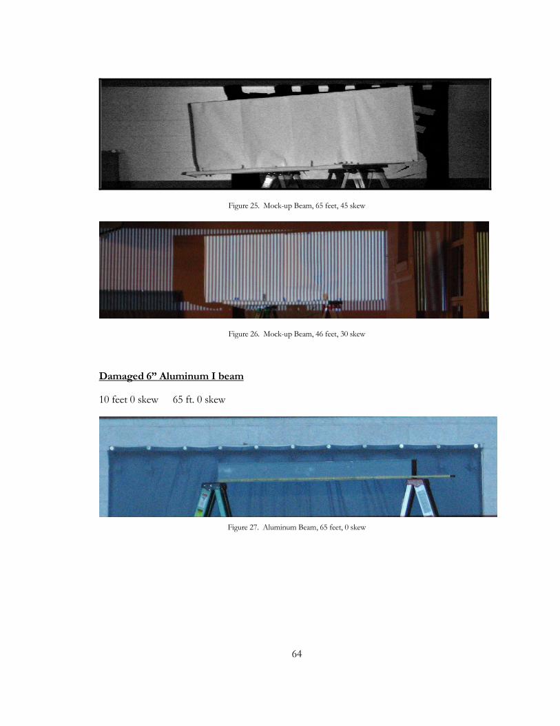
64
Figure 25. Mock-up Beam, 65 feet, 45 skew
Figure 26. Mock-up Beam, 46 feet, 30 skew
Damaged 6” Aluminum I beam
10 feet 0 skew 65 ft. 0 skew
Figure 27. Aluminum Beam, 65 feet, 0 skew

65
Figure 28. Aluminum Beam, 10 feet, 0 skew
Segments of deteriorated structural angles removed from the South End Bridge in
Agawam and Springfield, Massachusetts.
3 – 6”x6”x7/16” Angles Segments (A, B, C)
Figure 29. Angle Segment A
Figure 30. Angle Segment B

66
Figure 31. Angle Segment C
With each experiment I did not attempt to completely block out all other light sources
since at a real bridge location it would be impossible to block out light sources. Other light
sources would instead have to be filtered out during analysis with the background image
mentioned previously and if need be additional filtering techniques.
Coordination between PowerPoint and PSRemote worked well after several practice
attempts. Eventually, only 1 or 2 wasted shots occurred for each setup. To start the timed
fringe slides required waiting 2 or 3 seconds after the camera took a shot of the no fringe slide;
this ensured that the pictures would not be while the slides were changing. What also helped
to start the timed fringe was the built-in shutter speaker in the camera. The volume on the
shutter speaker can be turned up so the shutter sound can be heard from quite a distance away.
To setup the equipment took approximately 20 to 30 minutes. To move it around to
took equally as long. Breaking down the equipment took from 10 to 20 minutes. I estimate at
real bridge location it might take somewhat longer depending on site conditions.
The next chapter will discuss what to do with the approximately 340 megabytes of
information.

67
CHAPTER 4
ANALYSIS
The process of turning photographs into data is a journey fraught with twists, turns and
many choices that leads to an imperfect estimate of reality.
4.1 Introduction
The goal of analysis is an unwrapped phase map that can be post-processed into real units
of measure. The unwrapped phase map is an estimate of the true phase as it relates to surface
geometry (topography). A basic equation of the nonlinear function of phase (ψ ) is Eq. 4.1.
(4.1) ( ) ( ) ( ) επϑψ ++= tktt 2 where
( )( )
NoiseandError
FunctionForcingtotk
PhaseTruet
=
+−=
=
επππ
ϑ.2
In theory, if the forcing function, errors, and noise are removed then all that should be left is the
true phase. The reality is that the data and methods of removing the other components are not
perfect, so what we have is an estimated phase (Φ).
To calculate the estimated phase can be broken down into 3 parts.
1. Image formatting and noise removal.

68
2. Phase calculation.
3. Phase Unwrapping.
The rest of this chapter will be devoted to describing these three parts with the
experimental images obtained for Angle B described in Chapter 3. Recall that Angle B is a
deteriorated structural angle segment removed from the South End Bridge is which located
over the Connecticut River between Springfield and Agawam, Massachusetts. The images of
this angle were selected because there are some interesting analysis problems with this
specimen that are common conditions found in bridge inspection. The problems will be
discussed as they appear.
4.2 Image Formatting and Noise Removal
The procedure to obtain the images from the camera requires five steps;
1. Download Images
2. Convert from RAW to TIFF format
3. Crop Images
4. Remove Noise
5. Mask off Background
4.2.1 Download Images
Downloading images from the camera to the computer is straightforward. Attach the
camera to the computer via a USB cable, use a software program capable of reading the images
to transfer images. For my camera the program is ZoomBrowser EX by Cannon, Inc. To

69
transfer the RAW 7.1 Megapixel images from the camera to the computer took approximately
15 minutes.
4.2.2 Convert from RAW to TIFF format
Converting from the RAW to the TIFF format was accomplished with the ZoomBrowser
EX program. There are two parameters to consider for converting; one, 8-bit or 16- intensity
values, and two, linear or non-linear processing.
TIFF images are intensity value data arrays. Elements in the array have an integer intensity
value whose limits depend on the range selected. For 8-bit, the range of intensity values is
from 0 to 255. For 16-bit, the range of intensity values is from 0 to 65535. For the Angle B
images the 16-bit range was selected to provide a finer precision of intensity values and to be
able to select the type of processing for TIFF conversion.
The choice between non-linear and linear processing is available only for 16-bit range
intensity and is dependant upon the amount of image touchup desired. Linear processing
performs very little image touchup and the result is TIFF image data that is close to the actual
RAW image data. Non-linear processing produces images that are extensively altered and the
result is image data that is further away to the actual RAW image data. Linear processing was
selected for obvious reasons.
The TIFF images produced are 40.5 MB each. The main reason why the images are so big
is that the TIFF format structure requires that the image data be stored 3 times. Recall that
each RAW image is 2304 row x 3072 column data array. In the TIFF format each image is

70
2304 row x 9216 column data array. Fortunately, during image cropping the final size of each
image will be drastically reduced.
4.2.3 Crop Images
The goal of cropping images is to reduce the size of the image array as possible to save
storage space and shorten processing time.
Figure 32. Angle B 40.5 MB TIFF Image with all 2304 rows x 3072 columns.
Figure 32 shows that Angle B occupies very few rows and most but not all columns which
means that the remaining rows and columns can be cropped out. In addition, two-thirds of
the TIFF structure can be cropped out. The first third of the TIFF structure contains a
grayscale version of the image which is more than adequate for analysis. The cropped image is
760 rows x 2940 columns and is 2.81 MB in size (93% size reduction).

71
All 47 images must be cropped exactly the same way to perform the analysis. Rather than
opening up each image individually and ‘hand’ crop, the cropping process was incorporated
into a program I wrote called ImageProcess. The program, written in MATLAB, opens each
image, performs the cropping and saves each cropped image to a new file.
Figure 33. Angle B 2.81 MB Grayscale TIFF Image - 760 rows x 2940 columns.
4.2.4 Remove Noise
The nighttime environment that bridges are located in is filled with random incoherent
light that cannot be blocked out. The next best method to complete blackout is to subtract
the light noise.
The easiest method of light noise subtraction is to take an image of the object without the
projector light and subtract it from each fringe image. This method works as long as the noise
light on the object does not have an intensity value near the maximum value of 65535.
Subtracting light this high in intensity will wipe out part of the object’s image. It is likely that if
light noise were this high in intensity the fringe patterns would noticeably be obstructed.

72
Figure 34. No Projector Light Image (The image has been enhanced to make it visible).
Figure 35. Angle B Image with light noise subtracted out.
Subtracting the No Light Picture has been incorporated into the ImageProcess program.
4.2.5 Mask off Background
Ideally we want to only analyze data where our object exists in an image and ignore the rest
of the image. The problem is it is nearly impossible to write a computer program to ignore
unimportant data. The objects we want to study come in all shapes and sizes, and the images
are taken from various angles other than normal to the surface of the object.
The best method to removing the background is to create a mask array of 1’s and 0’s. The
mask array is, element by element, multiplied by each of our images. The result is our object in

73
a surrounded by a completely black background. One method to making a mask requires our
object to have the highest or nearly highest intensity (is the brightest or nearly brightest object)
values in the image. If this requirement is met, the mask is created by rounding to the nearest
integer the intensity value of each element divided by maximum intensity value.
(4.2) ( ) ( )
=
IntensityMax
jiIntensityroundjiMask
.
,,
The mask calculated in equation 4.2 will result in intensity values greater than or equal to
0.5 x Maximum Intensity. If the mask of EQ. 4.2 does not adequately address your masking
requirements the mask can be adjusted to preserve higher or lower intensity by adding an
adjustment term.
(4.3) ( ) ( )5.05.0
.
,, <<−
+= αα where
IntensityMax
jiIntensityroundjiMask
If the adjustment term ‘α’ is greater than 0 then the minimum intensity value to preserve
will be a value that is less than half the maximum intensity value. If the adjustment term ‘α’ is
less than 0 then the minimum intensity value to preserve will be a value that is greater than half
the maximum intensity value. The limits of the adjustment term ensures that mask values
never evaluate to anything other than 0 or 1.
What happends when the object you want is not the brightest or nearly the brightest
object? Take for instance Angle B (see fig. 30). Angle B is not the brightest object in fact,
nearly all intensity values found on Angle B are less than half the maximum intensity value. In

74
this situation we want to create a mask that sets the highest intensities to 0 and the lower
intensities to 1 (a negative mask). A modification to Eq. 4.3 can accomplish this.
(4.4) ( ) ( )5.05.01
.
,, <<−
−
+= αα where
IntensityMax
jiIntensityroundABSjiMask
Equation 4.4 was used for creating the initial mask for Angle B with α = +0.15. This
means that the highest 65% of intensity values were eliminated from the image. Equation 4.4
can also be called a spatial low pass filter. Low pass filters are used to eliminate high frequency
noise which is what the initial mask for Angle B is for. The mask for Angle B was further
enhanced by eliminating low intensity values and hand editing.
The elimination of low intensity values was accomplished by first creating a temporary
image array from the multiplication of the cropped no fringe image by the initial mask and
rescaling so that the maximum intensity value equaled the 16-bit limit of 65535. The rescaling
was performed as an attempt to create a greater separation between the object intensity values
and non-object intensity values. A new mask was created for the temporary image using Eq.
4.3 and an α = +0.425. This means that the lowest 7.5% of non-zero intensity values were
eliminated from the image.
Hand editing is the process of selecting particular areas of the mask to set to 0 or 1 that
can not be programmed. I performed hand editing in MATLAB by opening the no fringe image ,
comparing it to the mask image and writing down the areas in row and column notation that I
wanted to set. I added the hand edited areas to the ImageProcess program.

75
There are numerous other more sophisticated methods of masking and filtering in the
spatial domain or frequency domain through Fournier transforms. One method I did try is a
Gaussian Low Pass Filter in the frequency domain. The Gaussian filter produced similar
results. However, for Civil Engineers with little or no background in signal processing, I kept
the masking method because of its simplisticity.
After each of the Angle B images is masked off they are stored in new files and are ready
for phase calculation.
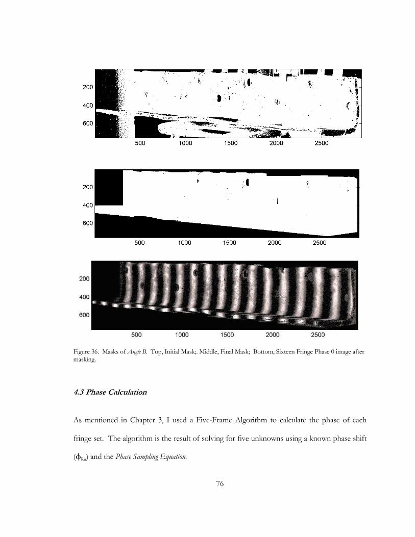
76
Figure 36. Masks of Angle B. Top, Initial Mask;. Middle, Final Mask; Bottom, Sixteen Fringe Phase 0 image after masking.
4.3 Phase Calculation
As mentioned in Chapter 3, I used a Five-Frame Algorithm to calculate the phase of each
fringe set. The algorithm is the result of solving for five unknowns using a known phase shift
(φRn) and the Phase Sampling Equation.

77
(4.5) ( ) ( ) ( )[ ] 3,..,.1,cos,, ≥=++= mmnwhereyxyxbyxaI Rnn φφ (Kreis 1996)
m = Number of images; n = frame number (0,1,2,3,4);
φ = Estimated Phase; a and b = additive and multiplicative distortions
The final estimated phase ( ( )nφ̂ is
(4.6) ( ) ( ) ( )[ ]( ) ( ) ( )
−+
−= −
2204
132tanˆ 1
III
IInφ (Rastogi 2001)
In a perfect world with a perfectly flat surface the resulting estimated phase would be 2π
wrapped perfectly as shown in figure 35a. However, in reality we have the wrapped phase
shown in figure 35b.
Besides real phase data being imperfect, there is another problem found on Angle B.
Notice at the far right in figure 35b at approximately column 2800, there appears to be
multiple discontinuities which would normally be an error. For Angle B it’s not a mistake, it’s a
rivet hole (see figure 36). The interior portions of holes have either been reduced to 0 through
masking and filtering, or they contain noise such as the hole shown in figure 36. Holes in an
object can cause problems in the phase unwrapping process which is the subject of the next
section in this chapter.

78
Figure 37. Top, Ideal Wrapped Phase of 1 Fringe; Bottom, Angle B Wrapped Phase of 1 Fringe for row 400 of array.

79
Figure 38. One Fringe Phase Map at (350:500, 2720:2900) with rivet hole.
4.4 Temporal Phase Unwrapping
Phase unwrapping is the key to producing usable information. Unfortunately, phase
unwrapping is the most difficult problem to solve. The main problem is developing an
algorithm that can accurately find 2π phase discontinuities. Numerous unwrapping
techniques have been developed over the last 25 years. Selecting a technique depends upon
the quality of the data to be analyzed. For Angle B a column-wise unwrapping would be
problematic due to the numerous errors and rivet holes along the column-wise phase path (see
figure 35b). Therefore, I selected a Temporal Phase Unwrapping technique to analyze Angle B.
Temporal Phase Unwrapping is a one-dimensional method that involves the unwrapping
of individual array elements (pixels) in the time dimension and independent of adjacent pixels.
Each pixel has three dimensions (x, y, and time). The advantage of this method is that random

80
pixels containing noise or pixels in rivet holes will not cause the unwrapping to fail. The
disadvantage is that it requires large volumes of data. Temporal algorithms rely on shifting the
fringe pattern either a constant or arbitrary step over time to minimize disturbances such as
vibrations on the object or wind vibrations on the equipment. The time period between
images of phase shifted fringes should be as short as possible. For Angle B each time
increment occurs with the change in fringe patterns therefore, the time increment can be set to
unity. The algorithm used here was first proposed by Huntley and Saldner in 1993 (Rastogi
2001).
4.4.1 Temporal Unwrapping Algorithm by Huntley and Saldner
( ) ( ) ( )[ ]{ }
( ) ( )
( ) ( ) ( )
( ) ( ) ( ) ( ) DifferencePhaseUnwrappedEsttvtt
PhaseUnwrappedEstimatedtvtt
tdtv
JumpsPhasettroundtd
WWU
UU
t
t
WW
.20ˆˆ0,ˆ)10.4(
2ˆˆ)9.4(
')8.4(
221ˆˆ(4.7)
'
←−−=∆
←−=
=
←÷−−=
∑
πφφφ
πφφ
ππφφ
The algorithm works by accumulating 2π jumps between successive times for each pixel
and then subtracting them out to unwrap the phase or calculate the unwrapped phase
difference.
The resulting phase maps should have a smooth uneven surface representing the objects
surface in phase values. In addition, there should be no fringes left. Maps meeting this criteria
can be post-processed into real units of measure. With this algorithm the difference between

81
the estimated phase and the phase difference map is the initial one fringe phase map. Either
map can be post-processed for use.
Figure 39. Wrapped 256 Fringe Maps at rows 1:760 x columns 1900:2600.
For Angle B, unwrapped phase map for fringes 1, 2, 4, 8 and 16 appear to have been
successfully unwrapped (see figures 40 and 41).
However, unwrapped phase maps for 32, 64, 128 and 256 fringes failed to unwrap successfully
(see figure 42).

82
Figure 40. Mesh Plot of Unwrapped Phase Maps shown for rows 1:300 x columns 1600:1800. Top Left, 1 fringe map. Top Right., map for up to 2 fringes. Bottom Left, up to 4 fringes. Bottom Right, up to 8 fringes.
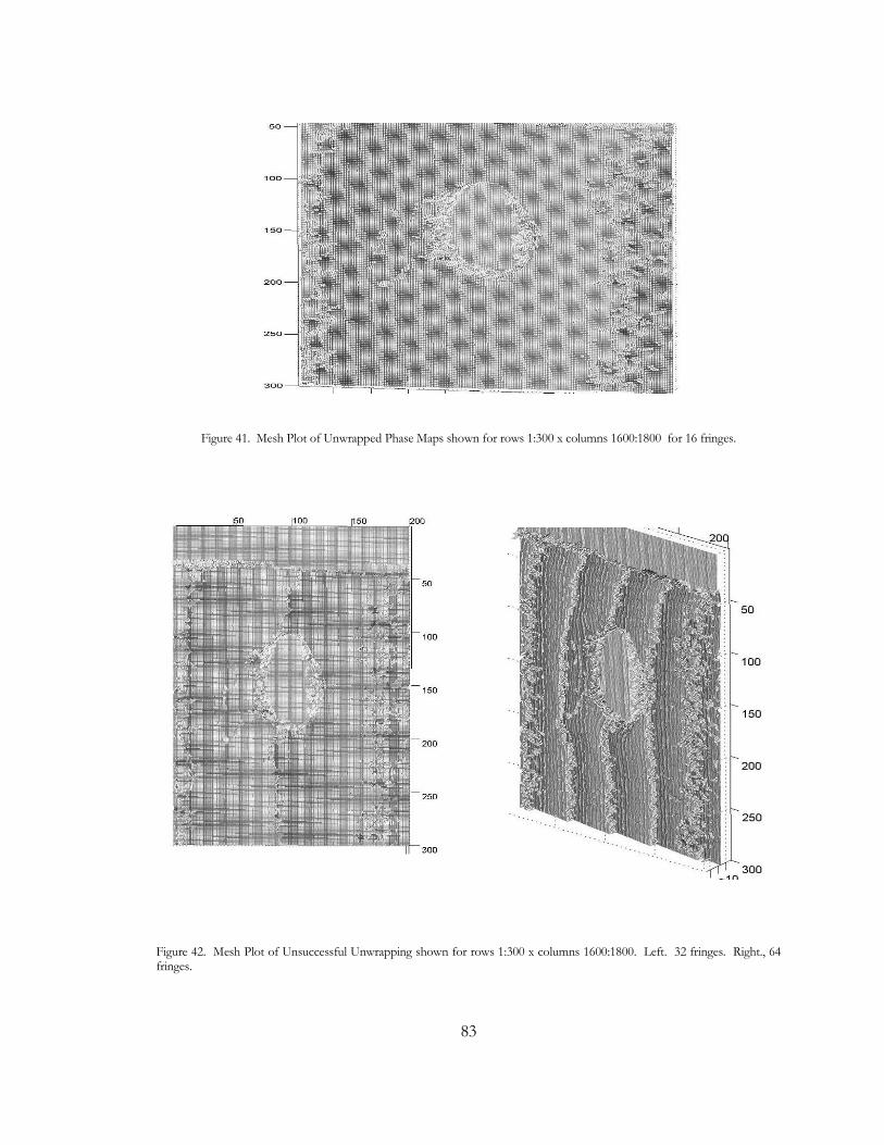
83
Figure 41. Mesh Plot of Unwrapped Phase Maps shown for rows 1:300 x columns 1600:1800 for 16 fringes.
Figure 42. Mesh Plot of Unsuccessful Unwrapping shown for rows 1:300 x columns 1600:1800. Left. 32 fringes. Right., 64 fringes.

84
Figure 43. Mesh Plot of Unsuccessful Unwrapping shown for rows 1:300 x columns 1600:1800. Left, 128 fringes. Right, 256 fringes.
Another algorithm proposed by Huntley, Kaufmann and Kerr in 1999, reportly produces a
smoother maps without removing discontinuous areas that are supposed to be in the map.
The algorithm calculates wrapped phase differences using a trigometric relationship instead of
simple subtraction.

85
4.4.2 Temporal Unwrapping Algorithm by Huntley, Kaufmann and Kerr
( )
( ) ( ) ( )[ ]{ }( ) ( )
( ) ( ) ( ) DifferencePhaseUnwrappedEstimatedtvtt
tdtv
JumpsPhasettroundtd
NNDD
NDDNtt
WU
t
t
WW
W
←−∆=∆
=
←÷−∆−∆=
+
−=∆
∑
−
πφφ
ππφφ
φ
20,ˆ0,ˆ)14.4(
')13.4(
220,1ˆ0,ˆ(4.12)
tan,ˆ (4.11)
'
1212
12121
12
For Angle B, unwrapped phase difference maps for accumulated differences up 2, 4, and
8 appear to have been successfully unwrapped (see figures 42 and 43). The difference map up
to fringe 16 appears to start deteriorating. The difference maps produced with the second
algorithm appear to be smoother than those of the first algorithm.
Figure 44. Mesh Plot of Unwrapped Phase Difference Map shown for rows 1:300 x columns 1600:1800 for accumulated differences to 2 fringes.

86
Figure 45. Mesh Plot of Unwrapped Phase Difference Map shown for rows 1:300 x columns 1600:1800 for accumulated differences to 8 fringes.
4.5 Column-Wise Phase Unwrapping
Another one-dimensional unwrapping method involves the unwrapping of rows of pixels
along the column dimension. Unlike temporal unwrapping the pixels are no longer
independently evaluated but evaluated row by row with each row being independent of
adjacent rows. The disadvantage of this method is that random pixels containing noise or
pixels in rivet holes will cause the unwrapping to fail. The advantage is that it requires only
five images to produce an unwrapped phase map. For this analysis, instead of Angle B, I used
the damaged aluminum beam images taken from 10 feet and normal to the beam. The
aluminum beam has no holes to contend with and the surface is smoother which should make

87
phase unwrapping easier. The algorithm used is based on general theories that can be found in
any text book on Interferometry. The algorithm’s 3 steps are;
1. Calculate the Fringe Order.
2. Remove 2π Discontinuities.
3. Remove the Fringe Pattern.
4.5.1 Calculate the Fringe Order
The Fringe Order are integer numbers that correspond to the regions of a wrapped phase
map between 2π discontinuities. The beginning and ending regions before the first and after
the last discontinuities are also part of the Fringe Order. The Fringe Order integers are 0,1,2,3,
etc. and are multipliers of 2π used to remove the discontinuities. Determining the column
limits of each Fringe Order consists of finding the 2π discontinuities of the wrapped phase.
Figure 46. Aluminum Beam, 4 Fringe Wrapped Phase, row 250

88
Figure 47. Aluminum Beam, 4 Fringe Order, row 250
4.5.2 Remove 2; Discontinuities
Removing the Discontinuities is simple matter of adding to the wrapped phase the product
of 2π times the Fringe Order. The result is a sloping image from left to right.
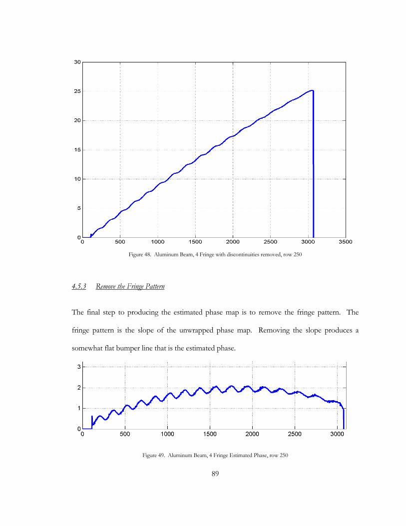
89
Figure 48. Aluminum Beam, 4 Fringe with discontinuities removed, row 250
4.5.3 Remove the Fringe Pattern
The final step to producing the estimated phase map is to remove the fringe pattern. The
fringe pattern is the slope of the unwrapped phase map. Removing the slope produces a
somewhat flat bumper line that is the estimated phase.
Figure 49. Aluminum Beam, 4 Fringe Estimated Phase, row 250

90
Figure 50. Aluminum Beam, Image, rows 50:150 x columns 300:500, note: lettering of wooden capenters ruler
Figure 51. Aluminum Beam, 4 Fringe Estimated Phase, rows 50:150 x columns 300:500, note: embossed lettering of wooden capenters ruler (embossing depth is less than 1 mm).
The phase calculations and unwrapping procedures were written into a MATLAB program call
Fringe. With the production of the Unwrapped Phase Map, the analysis is complete.

91
C O N C L U S I O N S
I started out with the idea of developing a new inspection tool that could be used by as
many bridge inspectors as possible. I established goals and requirements for such a tool. I
compared the inspection tool to traffic engineering data collection and analysis where there is a
separation between the two tasks. The data collectors have the simple job and the engineers
have the complex job. I believe that I can say that the bridge inspection tool based on
interferometry, also separates data collection (easier task) from analysis (complex tasks).
The field work of taking the images (data collection) appears to be easier than I had
originally thought. After a dozen or so setups and image acquisitions it almost seems routine.
Bridge inspectors would have no problem learning to use this tool.
The analysis work, on the other hand, is more difficult and time consuming then first
thought. Understanding how interferometry works takes time, especially someone with no
signal processing background. The following is a list of observations about analysis;
Sources of Fringe Unwrapping Failure
In all of my experiments (the ones included in my thesis and others) the higher numbers of
fringes failed to produce acceptable results. Possible causes are resolution of equipment,
resolution differences between equipment, and fringe projection images.

92
Resolution of Equipment: There are three components that the resolution limit could
cause failure; the camera, projector and fringe images.
The camera resolution is the highest and I assume does not contribute significantly to
fringe failure. Higher resolution cameras are readily available and their costs keep dropping.
The projector resolution appears to be the controlling influence on the tool. Projectors are
expensive and finding higher resolution projectors that are portable and economical is a
challenge. Perhaps an investigation into finding alternative means of projecting fringes at
greater distances would be beneficial.
The fringe images I used were 768 x 768 TIFF images. That means any fringe projection
would have to fit within those 768 columns. For one fringe there are plenty of data points to
produce the sinusoidal wave. But for 256 fringes there are only 3 data points to describe an
entire fringe. The resulting image is a saw tooth pattern not a sinusoidal wave. A way of
determining the resolution ability of a certain sized fringe would be to adhere to the rule that at
least 10 data points are necessary per fringe. In my experiments, the highest number of fringes
should be 64 (768/10 = 76.8). But my 64 fringes did not work, so something else is limiting
the number of fringes.
Resolution Differences Between Equipment: The camera, projector and fringe image all
have different resolutions. The fringe image has 768 columns, the projector has 1280 columns
and the camera has 3072 columns. How are lower resolution images expended out to higher
resolution images within a computer and how are handled by the camera? We can remove one

93
resolution problem by producing fringe images to the column resolution of the projector
resolution; in theory this should produce better results.
Fringe Projection Images: In theory, the fringe projection images we produce
mathematically should, if one wanted to calculate the wrapped phase of them, produce a
perfect wrapped phase. The exception might be when there are fewer than 10 data points per
fringe as mentioned above. But the real questions are; will 10 produce perfect results? If not,
how many data points does it take to reach perfection? I wrote a sinusoidal fringe generator
program in MATLAB™, generated fringes some fringes with varying numbers of data points.
Then I calculated the wrapped phase using my fringe program.
Data Points Max. Positive Max. Negative My Fringe Number
3 2.0944 -2.0944 256
6 π -2.0944 128 12 π -2.6180 64 24 π -2.8798 32 48 π -3.0107 16 96 π -3.0761 8 192 π -3.1089 4 384 π -3.1252 2 768 π -3.1334 1
I back checked the results above in a spreadsheet program and came up with the same results.
It is not hard to figure out why my phase unwrapping fell apart after or at 16 fringes. I was
looking for legitimate 2π discontinuities and there were none to be found. I carried out the
fringe calculation to 6144 data points (twice the resolution of my camera) and got -3.1406.

94
Either the method to produce fringes needs to be modified or maybe a different wrapped
phase algorithm requiring a different number of images should be researched.
Other Insights
The research presented in this thesis demonstrated most but not all the steps of using a
new technology solve an old problem. The last step, post processing of the unwrapped phase
map, was not presented here since it would encompass another thesis by itself.
Post processing research would include correcting the distortions caused by the lenses of
the camera and the projector, creating a relational lookup table between the phase values and
real units of measure, and developing a relationship between the geometry of the
interferometry apparatus setup and the pixel rows and columns.
In addition to post processing, other further research needs include equipment, software,
and actual bridge experiments.
The equipment used in this thesis was a modified version of setup already in use. For
bridge inspection use, research should be conducted into using separated camera and projector
stands instead of the rigid mounting bar setup. Bridges are not laboratory specimens that can
be moved in relation to the equipment; they are large immovable objects situated in an
environment hostile to rigidly configured equipment. By allowing variability in the distance
between the camera and projector will allow for optimum data collection at any bridge
location.

95
In addition to post processing, software research would include developing a single
program for camera and projector control, and splicing together separate adjacent phase maps.
A single program to control the projector slide show and the camera would remove the
tricky coordination of running two programs simultaneously. The PSRemote program does
have interface routines written in C++ so that other programs can trigger the camera.
Writing a program to splice together phase maps goes beyond producing a panoramic
map; it can be written to be a correction tool. At a bridge, any large bridge member will likely
require multiple image sets and the image sets will not be taken at the same distance from the
bridge. This means that one image set will be closest to the bridge and one image set will be
furthest away from the bridge. The closest set will produce the most accurate phase map while
the furthest set will produce the most inaccurate phase map. Therefore, we could use the
closest phase map to correct adjacent and overlapping phase maps in addition to splicing the
phase maps together.
Setting up the equipment at an actual bridge was attempted but failed due an equipment
problem. I do intend, in the near future, to try again. Research into field trials of equipment
should first be directed at bridge members with large deformations and extensive deteriorated
areas. The best candidates would be bridges that have collision damage. Very little research
has been performed on the nature of bridge collision damage and data collection of damage is
primitive. The large deformations due to collisions usually occur on the most easily accessible
bridge components (for example fascia beams) and deformations should be highly visible in
the phase maps.

96
Lastly, this thesis has been a journey through the last frontier of data acquisition,
photography. The ability to breakdown an inanimate object into usable data opens up a world
of potential for all of Civil Engineering and not just bridge inspection.

97
REFERENCES
Barson, John M., and Stanley T. Rolf. Fracture and Fatigue Control in Structures: Applications
of Fracture Mechanics. 2nd ed. Englewood Cliffs, NJ: Prentice-Hall, 1987.
Bolukbasi, Melik, Jamshid Mohammadi, and David Arditi. Estimating the Future Condition of
Highway Bridge Components Using National Bridge Inventory Data. Practice Periodical on
Structural Design and Construction 9.1 (2004): 16-25.
Brockenbrough, Roger L. AISC Rehabilitation and Retrofit Guide: A Reference for Historic
Shapes and Specifications. Chicago: American Institute of Steel Construction, 2002. Vol.
15 of Steel Design Guide Series.
Chase, Steve B. High-Tech Inspection. Civil Engineering Magazine 71.9 (2001): 62-65.
Estes, Allen C., and Dan M. Frangopol. Updating Bridge Reliability Based on Bridge Management
Systems Visual Inspection Results Journa l of Bridge Engineering 8.6 (2003): 374-382.
Fisher, John W. Fatigue and Fracture in Steel Bridges: Case Studies. New York: John Wiley
and Sons, 1984.
Fong, Philip and Florian Buron. "Sensing Moving and Deforming Objects with Commercial
Off the Shelf Hardware," IEEE International Workshop on Projector-Camera Systems
(PROCAMS), June 2005, San Diego CA, USA
Ghiglia, Dennis C., and Mark D. Pritt. Two-Dimensional Phase Unwrapping: Theory,
Algorithms, and Software. New York: John Wiley and Sons, 1998.
Gonzalez, Rafael C., Richard E. Woods, and Steven L. Eddins. Digital Image Processing using
MATLAB. Singapore: Parsons Education, 2004.
98
Jacquot, P., and M. Facchini. Interferometric Imaging: Involvement in Civil Engineering. Journal of
Computing in Civil Engineering 13.2 (1999): 61-70.
Kreis, Thomas. Holographic Interferometry: Principles and Methods. Berlin, Germany:
Akademie Verlag, 1996. Vol. 1 of Akademie Verlag Series in Optical Metrology.
LeRose, Chris. The Collapse of the Silver Bridge. West Virginia Historical Society Quarterly. 15.4
(2001)
Martinez-Celorio, R.A., A. Davila, B. Barrientos, J.H. Puga, and Luis Marti Lopez. Matched
spatial-phase-shifting for the temporal-phase-unwrapping in electronic speckle pattern interferometry.
International Journal for Light and Electron Optics 112.11 (2001) : 515-520.
Massachusetts Highway Department. BMS Element Data Collection Manual. September, 1995.
McCullough, David. The Great Bridge: The Epic Story of the Building of the Brooklyn
Bridge. New York: Simon & Schuster, 1972; Touchstone Books. First Edition, 1982.
National Transportation Safety Board. Highway Accident Report: Collapse of U.S. 35 Highway
Bridge, Point Pleasant, West Virginia: December 15, 1967. Adopted December 16,
1970. NTSB, HAR - 71/01, NITS, PB - 190202.
---. Highway Accident Report: Collapse of a Suspended Span of Route 95 Highway Bridge over
the Mianus River, Greenwich, Connecticut: June 28, 1983. Adopted: July 19. 1984.
NTSB, HAR -84/03, NITS, PB84 - 916203.
---. Highway Accident Report: Collapse of New York Thruway (I-90) Bridge Schoharie Creek
near Amsterdam, New York, April 5, 1987. NTSB, HAR - 88/02, NITS, PB88 -
916202.

99
---. Highway Accident Report: Collapse of the Northbound U.S. Route 51 Bridge Spans over the
Hatchie River Near Covington, Tennessee, April 1, 1989. NTSB, HAR - 90/01, NITS,
PB91 - 916201.
Phares, Brent M., Glenn A. Washer, Dennis D. Rolander, Benjamin A. Graybeal, and Mark
Moore. Routine Highway Bridge Inspection Condition Documentation Accuracy and Reliability.
Journal of Bridge Engineering 9.4 (2004): 403-413.
Rastogi, Pramod K., ed. Digital Speckle Pattern Interferometry and Related Techniques.
Chichester, West Sussex, England: John Wiley and Sons, 2001
Railroad Museum of New England. The Naugatuck Railroad - a Historical Background.
Thomaston, CT. Copyright, 2003.
Sansoni, Giovanna, Alessandro Patrioli, and Franco Docchio. OPL-3D: A novel, portable optical
digitizer for fast acquision of free-form surfaces. Review of Scientific Instruments 74.4 (2003):
2593-2603.
Silano, Louis G., ed. Bridge Inspection and Rehabilitation: A Practical Guide. New York: John Wiley and Sons, 1993.
Sitnik, Robert, Matgorzata Kujawinska, and Jerzy Woznicki. Digital fringe projection system for
large-volume 360-deg shape measurement. Optical Engineering 41.2 (2002) : 443-449.
---. Phase scaling using characteristic polynominals. Proceedings of the Society of Photo-Optical
Instrumentation Engineers 5532 (2004) : 211-217.
U.S. Department of Transportation: Federal Highway Administration. Bridge Inspector’s
Reference Manual (BIRM). Washington, DC: U.S. Government Printing Office, 2002.
---. Bridge Inspector’s Training Manual (Manual 90), Report No. FHWA-PD-91-015.
Washington, DC: U.S. Government Printing Office, 1995.
100
---. Bridge Inspector’s Training Manual (Manual 70). Washington, DC: U.S. Government
Printing Office, 1979.
---. Highway Bridge Inspection: State-of-the-Practice Study, Report No. FHWA-RD-01-033.
Washington, DC: U.S. Government Printing Office, 2001.
---. Inspection of Fracture Critical Bridge Members: Supplement to the Bridge Inspector’s
Training Manual, Report No. FHWA-IP-86-26. Washington, DC: U.S. Government
Printing Office, 1986.
---. Reliability of Visual Inspection for Highway Bridges, Volume I: Final Report, Report No.
FHWA- RD-01-020. Washington, DC: U.S. Government Printing Office, 2001.
U.S. Government. Code of Federal Regulations, Title 23, Chapter 1, Section 650.3 (National
Bridge Inspection Standards).
Vose, George L. Bridge Disasters in America: The Cause and the Remedy. Boston: Lee and
Shepard, 1887.
Wardhana, Kumalasari, and Fabian C. Hadipriono. Analysis of Recent Bridge Failures in the United
States. Journal of Performance of Constructed Facilities 17.3 (2003): 144-150.
Whittle, D.W., ed. “ Chapter 24 - Ashtabula Bridge Disaster.” Memoirs of Philip P. Bliss.
New York: A.S. Barnes and Co., 1877. pp. [290]-296.

101
APPENDIX A - COMPUTER PROGRAMS
% Image Processing Program % This program 1. input 40 meg. tiff files. % 2. crop image to remove waste areas. % 3. Subtract Background Image. % 3. Create Mask File from no fringe image. % 4. Mask out background. % 5. new tiff image will be gray scale only (1/3 rd % size). % 6. save image in new file with % rootfilename + fringe # + phase # + .tif filenameroot = 'ALBeam65ft0sk'; % input file root name m1 = 1101; m2 = 1220; n1 = 1; n2 = 3072; i1 = 3; i2 = 47; % Background Image % Infile = imread(strcat(filenameroot,'47.tif')); % open background image % background(:,:) = double(Infile(m1:m2,n1:n2,1)); % crop background to match other images % imwrite(uint16(background),[filenameroot,'bckgrnd.tif']); % clear Infile; % axes('DataAspectRatio',[1 1 1]); % imagesc(background) % pause % % Create Mask % Infile = imread(strcat(filenameroot,'48.tif')); % open no fringe image % temp(:,:) = double(Infile(m1:m2,n1:n2,1)); % crop mask to match other images % [mmax,nmax] = size(temp); % maxintensity = max(max(temp)); % % Mask = abs(round(temp / maxintensity) - 1); % % Mask = abs(round(temp / maxintensity + 0.15) - 1); % Mask for removing highest intensity values. % temp = temp .* Mask; % Remove Highest intensities.
102
% % temp = temp * 65535 / max(max(temp)); % Rescale Intensity values remaining. % % % Mask = round(temp / max(max(temp)) + 0.425); % Set mask values to 1 or 0 % % imagesc(Mask) % pause % % % hand determined masking areas % % Mask(660:750,2480:2880)=abs(round(temp(660:750,2480:2880)/45000)-1); % % Mask(430:520,250:1500) = 1; % Mask(500:550,750:2000) = 1; % Mask(540:580,1250:1650) = 1; % Mask(100:660,2800:end) = 1; % % Mask(1:65,2290:end) = 0; % Mask(1:70,1910:2290) = 0; % Mask(1:80,2590:end) = 0; % Mask(1:6,1:end) = 0; % Mask(1:400,1:315) = 0; % Mask(1:end,2920:end) = 0; % % for i=485:mmax % Mask(i,1:round((i-485)*10)) = 0; % end % for i=6:64 % Mask(i,round(430+(i-6)*45):end) = 0; % end % for i=694:mmax % Mask(i,round(nmax-(i-694)*7):end) = 0; % end % % clear temp; % % imagesc(Mask) % pause % % imwrite(uint16(Mask),strcat(filenameroot,'mask.tif')); % clear Infile; % process fringe images Fringe = 1; Phase = 0; for i = i1:i2 % filename = [filenameroot,num2str(Fringe),num2str(Phase),'.tif']; if i<10 filename = [filenameroot,'0',num2str(i),'.tif']; else filename = [filenameroot,num2str(i),'.tif'];

103
end Infile = imread(filename); Outfile(:,:) = uint16(Infile(m1:m2,n1:n2,1)); % Crop Image. Taking only the first image 1:3072 max. if Phase == 0 filename = ['x',filenameroot,num2str(Fringe),num2str(Phase),'a.tif']; imwrite(Outfile,filename,'tif'); end % Outfile(:,:) = uint16(double(Outfile(:,:)) - background(:,:)); % Subtract background noise % % if Phase == 0 % filename = ['x',filenameroot,num2str(Fringe),num2str(Phase),'b.tif']; % imwrite(Outfile,filename,'tif'); % end % % Outfile(:,:) = uint16(double(Outfile(:,:)) .* Mask(:,:)); % Mask out background % % if Phase == 0 % filename = ['x',filenameroot,num2str(Fringe),num2str(Phase),'m.tif']; % imwrite(Outfile,filename,'tif'); % end filename = [filenameroot,'bm',num2str(Fringe),num2str(Phase),'.tif']; imwrite(Outfile,filename,'tif'); if Phase > 3 Phase = 0; Fringe = Fringe * 2; else Phase = Phase + 1; end clear Infile Outfile filename; end

104
% Fringe Interferometry Program % Initialize Section format compact; warning off MATLAB:divideByZero; warning off MATLAB:nearlySingularMatrix % Input Number of Frames and Size % ------------------------------------------------------------------------- prompt1 = {'Enter input file root:',... 'Enter input file extension:',... 'Enter the size of input images (rows columns):',... 'Enter bit size (Ex: 8 bit, 16 bit, etc.):',... 'Enter number of fringe sets',... 'Enter lowest number of fringes:',... 'Enter number of fringe phases:'}; dlg_title = 'Input for Frames'; answer = inputdlg(prompt1,dlg_title,1); fileroot = cell2mat(answer(1)); fileExt = cell2mat(answer(2)); mn = cell2mat(answer(3)); %separate m & n and change them into numbers place = strfind(mn,' '); msize = str2num(mn(1:place-1)); nsize = str2num(strrep(mn,[mn(1:place-1),' '],'')); bits = cell2mat(answer(4)); bits = ['uint',bits]; numsets = str2num(cell2mat(answer(5))); lowfringe = str2num(cell2mat(answer(6))); numfrph = str2num(cell2mat(answer(7))); clear prompt1 mn place % ------------------------------------------------------------------------- % Main Program % ------------------------------------------------------------------------- m = msize; n = nsize; for N = 1:numsets if lowfringe > 0 fringenum = num2str(lowfringe*2^(N-1)); else if N > 1 fringenum = num2str(2^(N-2));

105
else fringenum = '0'; end end for j = 1:numfrph % construct input file name framename = [fileroot,fringenum,num2str(j-1),'.',fileExt]; % Open frame file %------------------------------------------------------------------------------- Inframe = imread(framename); framestore(1:msize,1:nsize,j) = Inframe; clear Inframe; end %----------------------------------------------------------------------------------- % phase and modulation by Five Frame Algorithm s = log2(str2num(fringenum)) + 1; % calculate storage number [D2,N2] = fiveframe(framestore); clear framestore; wrapmap(:,:,s) = angle(complex(D2,N2)); % ATAN in the +pi -pi range %clear D2 N2; %----------------------------------------------------------------------------------- % Temporal Phase Unwrapping % % Temporal Unwrapping Algorithm 1 - Section 2.4.1.1 % on page 102 of "Digital Speckle Pattern Interferometry and % Related Techniques", Edited by Pramod K. Rastogi, John Wiley and Sons, LTD, % West Sussex, England, 2001 % ---------------------------------------------------------------------------------- % if N == 1 % d = round(wrapmap(:,:,s)/2/pi); % v = d; % else % d = round((wrapmap(:,:,N) - wrapmap(:,:,N-1))/2/pi); % v = v + d; % end % % unwrapmap(:,:,s) = wrapmap(:,:,s) - 2*pi*v; % %deltaunwrapmap(:,:,s) = wrapmap(:,:,s) - wrapmap(:,:,1) - 2*pi*v;

106
% % % ----------------------------------------------------------------------------------- % end %----------------------------------------------------------------------------------- % Temporal Phase Unwrapping % % Temporal Unwrapping Algorithm 3 - Section 2.4.1.3 % on page 104 of "Digital Speckle Pattern Interferometry and % Related Techniques", Edited by Pramod K. Rastogi, John Wiley and Sons, LTD, % West Sussex, England, 2001 % ---------------------------------------------------------------------------------- if N == 1 d = zeros(m,n); v = d; delta2 = zeros(m,n); else delta2 = angle(complex((D2.*D1 + N2.*N1),(N2.*D1 - D2.*N1))); % equation 2.52 page 95 d = round((delta2(:,:) - delta1(:,:))/2/pi); v = v + d; end deltaunwrapmap(:,:,s) = delta2(:,:) - 2*pi*v; delta1 = delta2; N1 = N2; D1 = D2; % ----------------------------------------------------------------------------------- end

107
% COLUMN-WISE PHASE UNWRAPPING % Input Area % Open wrapmap table into MATLAB [msize, nsize,sets] = size(wrapmap); N = 1; % Main Program numfringe = 2^(N-1); range = round(3072/numfringe/2); Order = zeros(msize,nsize); for i = 1:msize j = 1; while wrapmap(i,j,N) == 0 && j < nsize-1 j = j + 1; end while j < nsize j = j + round(range*3/4); while j < nsize-1 && wrapmap(i,j,N)-wrapmap(i,j+1,N)< 1.999*pi j = j + 1; end if j<nsize Order(i,j+1+5:end) = Order(i,j+1+5:end) + 1; end end end unwrapmap(:,:,N) = wrapmap(:,:,N) + 2*pi*Order; step = numfringe*2*pi/3072; for i = 1: msize j = 1; while unwrapmap(i,j,N) <= 0 && j < nsize j = j + 1; end if j <= nsize flat(i,1:j,N) = unwrapmap(i,1:j,N); for jj = j:nsize flat(i,jj,N) = unwrapmap(i,jj,N) - step*(jj-j); end j = nsize; while unwrapmap(i,j,N)==0 && j >1 flat(i,j,N) = 0; j = j - 1; end end end

108
function [D,Ni] = fiveframe(framein); % function to calculate estimated phase and modulation by % Five Frame Algorithm % Section 2.2.1.2 on pages 66 & 67 of "Digital Speckle Pattern Interferometry - % and related Techniques", edited by Pramod K. Rastogi, John Wiley and Sons, LTD, % West Sussex, England, 2001 % --------------------------------------------------------------------- [m,n,numsets] = size(framein); f0(1:m,1:n) = double(framein(1:m,1:n,1)); f1(1:m,1:n) = double(framein(1:m,1:n,2)); f2(1:m,1:n) = double(framein(1:m,1:n,3)); f3(1:m,1:n) = double(framein(1:m,1:n,4)); f4(1:m,1:n) = double(framein(1:m,1:n,5)); D = f4+f0-2*f2; % Real Part Ni = 2*(f3-f1); % Imaginary Part %Phase = angle(complex(D,Ni)); %Im = (4*(f3-f1))^2+(f4+f0-2*f2)^2)^0.5/4; %Im = uint8(Im);
%Im = 1;