Embed Size (px)
Citation preview
USE OF GROUND-BASED CANOPY REFLECTANCE TO DETERMINE
RADIATION CAPTURE, NITROGEN AND WATER STATUS,
AND FINAL YIELD IN WHEAT
by
Glen L. Ritchie
A thesis submitted in partial fulfillment
for the requirements of the degree
of
MASTER OF SCIENCE
in
Plant Science (Crop Physiology)
Approved: ____________________ ____________________ Bruce Bugbee V. Philip Rasmussen Major Professor Committee Member _____________________ _____________________ Esmaiel Malek Robert R. Gillies Committee Member Committee Member
_____________________ Thomas Kent
Dean of Graduate Studies
UTAH STATE UNIVERSITY Logan, Utah
2003
ii
Copyright © Glen Ritchie 2003
All Rights Reserved

iii
ABSTRACT
USE OF GROUND-BASED CANOPY REFLECTANCE TO
DETERMINE GROUND COVER, NITROGEN AND WATER STATUS,
AND FINAL YIELD IN WHEAT
by
Glen L. Ritchie, Master of Science
Utah State University, 2003
Major Professor: Dr. Bruce Bugbee Department: Plants, Soils, and Biometeorology
Ground-based spectral imaging devices offer an important supplement to
satellite imagery. Hand-held, ground-based sensors allow rapid, inexpensive
measurements that are not affected by the earth’s atmosphere. They also
provide a basis for high altitude spectral indices.
We quantified the spectral reflectance characteristics of hard red spring
wheat (Triticum aestivum cv. Westbred 936) in research plots subjected to either
nitrogen or water stress in a two year study. Both types of stress reduced ground
cover, which was evaluated by digital photography and compared with ten
spectral reflectance indices. On plots with a similar soil background, simple
indices such as the normalized difference vegetation index, ratio vegetation
index, and difference vegetation index were equal to or superior to more complex
vegetation indices for predicting ground cover. Yield was estimated by

iv
integrating the normalized difference vegetation index over the growing season.
The coefficient of determination (r2) between integrated normalized difference
vegetation index and final yield was 0.86.
Unfortunately, none of these indices were able to differentiate between the
intensity of green leaf color and ground cover fraction, and thus could not
distinguish nitrogen from water stress. We developed a reflective index that can
differentiate nitrogen and water stress over a wide range of ground cover. The
index is based on the ratio of the green and red variants of the normalized
difference vegetation index. The new index was able to distinguish nitrogen and
water stress from satellite data using wavelengths less than 1000 nm. This index
should be broadly applicable over a wide range of plant types and environments.
(134 pages)

v
ACKNOWLEDGMENTS
I would like to thank Bruce Bugbee, an exceptional scientist, teacher, and
friend, for the opportunity to learn in his lab. I would also like to thank the other
members of my committee. Rob Gillies provided several valuable and unique
insights during the editing of this thesis, Esmaiel Malek taught me several
valuable fundamentals that relate directly to this work, and Phil Rasmussen
provided expert advice, leadership, and the grant that funded my project.
I would also like to thank everyone in my family, particularly Mom, Dad,
Karl, Kathryn, Melanie, Renae, Pam, and their families, for not losing hope during
difficult times. The stars shine brightest on the darkest nights.
I would be remiss if I did not acknowledge some of the others who have
worked with me, helped me, taught me, and made me laugh during the past
three years. Dan Dallon, Dennis Wright, Giridhar Akula, and Nate McBride all
helped me with several important aspects of my research. Jonathan and Susan
Frantz, Julie and Brandon Chard, Derek Pinnock, Steve Klassen, Amelia Henry,
and everyone else in the Crop Physiology Lab also helped turn my thesis into
what it is. Thanks.
I especially want to thank my beautiful wife, Kristina, for standing beside
me during almost three years of thesis research, and for putting up with two
active children while I did my research. Thanks to Brandon and Erin for giving us
a new outlook on life.
Glen Ritchie

vi
CONTENTS
Page ABSTRACT ........................................................................................................ iii ACKNOWLEDGMENTS ....................................................................................... v LIST OF TABLES .................................................................................................ix LIST OF FIGURES ............................................................................................... x CHAPTER 1. INTRODUCTION................................................................................. 1 OVERVIEW......................................................................................... 1 OBJECTIVES...................................................................................... 2 REFERENCES.................................................................................... 3 2. LITERATURE REVIEW....................................................................... 5 LEAF INTERACTIONS WITH VISIBLE AND NEAR-
INFRARED RADIATION ................................................................. 5 MEASURING PLANT/RADIATION INTERACTIONS.......................... 7 Definitions of Reflectance, Transmittance, and Absorbance........... 7 Instrumentation ............................................................................... 7 Leaf Reflectance and Plant Stress .................................................. 9 Growth Stage and Canopy Geometry ........................................... 12 Sensor angle................................................................................. 12 Solar angle and time of day .......................................................... 13 Ground cover and the soil background ......................................... 14 CURRENT SATELLITE CAPABILITIES............................................ 15 SPECTRAL INDICES........................................................................ 16 Ratio and Difference Vegetation Indices ....................................... 17 Soil-Adjusted Vegetation Indices................................................... 18 Derivative Indices.......................................................................... 19 Band Depth Analysis..................................................................... 24 REFERENCES.................................................................................. 25
vii
3. DEVELOPMENT OF A NOVEL SPECTRAL REFLECTIVE INDEX TO DIFFERENTIATE NITROGEN AND WATER STRESS FROM EMERGENCE TO CANOPY CLOSURE................ 31
ABSTRACT................................................................................... 31 INTRODUCTION........................................................................... 32 Methods for Estimating Ground Cover..................................... 34 Spectral Indicators of Plant Color ............................................ 37 MATERIALS AND METHODS ...................................................... 41 RESULTS ..................................................................................... 45 Comparison of Indices to Measure Ground Cover................... 45 Differentiating N and Water Stress .......................................... 47
Identifying Plant Chlorosis Using Normalized Green and Red Reflectance ........................................................................ 48
Using the NGR Relationship to Identify Water Stress.............. 58 Identification of N Stress from Satellite Data............................ 61 DISCUSSION................................................................................ 63 Advantages of the NGR Relationship ...................................... 63 Effects of Solar Angle .............................................................. 63 Comparison of Spectral Indices with Chlorophyll Content ....... 64 Satellite Data and the NGR Relationship................................. 65 Comparison of 2001 and 2002 unstressed lines...................... 65 CONCLUSIONS............................................................................ 66 4. SUMMARY........................................................................................ 70 APPENDICES APPENDIX 1: PREDICTING GROUND COVER AND YIELD ................. 73 ABSTRACT................................................................................... 73 INTRODUCTION........................................................................... 74 MATERIALS AND METHODS ...................................................... 77 RESULTS AND DISCUSSION...................................................... 80 REFERENCES.............................................................................. 87 APPENDIX 2: LEAF REFLECTANCE, TRANSMITTANCE, AND
CHLOROPHYLL CONCENTRATION ............................................... 90

viii
ABSTRACT....................................................................................... 90 INTRODUCTION............................................................................... 90 MATERIALS AND METHODS .......................................................... 92 RESULTS….. .................................................................................... 93 DISCUSSION.................................................................................... 96 REFERENCES.................................................................................. 96 APPENDIX 3: BACKGROUND EFFECTS ON SPECTRAL
INDICES ........................................................................................... 98 ABSTRACT....................................................................................... 98 INTRODUCTION............................................................................... 99 MATERIALS AND METHODS ........................................................ 100 RESULTS ....................................................................................... 104 DISCUSSION.................................................................................. 107 REFERENCES................................................................................ 108 APPENDIX 4: SOLAR ANGLE AND VEGETATION INDICES ............. 110 ABSTRACT..................................................................................... 110 INTRODUCTION............................................................................. 110 MATERIALS AND METHODS ........................................................ 113 RESULTS ....................................................................................... 116 REFERENCES................................................................................ 116 APPENDIX 5: GRAPHS AND STATISTICS FOR NITROGEN AND
WATER-STRESS PAPER .............................................................. 118 APPENDIX 6: GRAPHS OF DVI, RVI, NDVI, AND GNDVI
COMPARED WITH DIGITAL IMAGES OF GROUND COVER....... 122
ix
LIST OF TABLES
Table Page
1 Visible and NIR absorption features that have been related to particular foliar chemical concentrations. ................................................... 6
2 Current and planned satellites with features pertinent to reflectance measurements. ........................................................................................ 15
3 Broad-band and narrow-band vegetation indices that are widely used for ground cover determination ....................................................... 35
4 Comparison of ratio and difference vegetation indices with digital images of ground cover collected during the entire growing season ....... 46
5 Statistical parameters of the 2001 and 2002 regression equations used to test whether the slopes are different ........................................... 52
6 Summer 2002 treatments ........................................................................ 77
7 Comparison of final yield with in-season NDVI values during 2001. ........ 81
8 Relationship between NDVI and final yield during 2002 by date.............. 84
9 Comparison of narrowband and broadband indices with leaf area index (LAI). ............................................................................................ 104
10 Statistical parameters of the 2001 and 2002 regression equations used to estimate whether the slopes are different. ................................ 121

x
LIST OF FIGURES
Figure Page
1 Typical visible and NIR plant reflectance. ................................................ 10
2 Using the linear nature of soil reflectance to eliminate soil background signal using derivatives of reflectance spectra. .................... 20
3 Use of a local baseline with 1st order derivative spectra to eliminate soil background signal .............................................................. 22
4 Comparison of derivative green cover estimates with common non-derivative vegetation indices to estimate LAI with different background colors ................................................................................... 23
5 Experiment design of wheat test plots with line source sprinkler system. .................................................................................................... 41
6 Comparison of NDVI with ground cover (measured by a digital camera) over time.................................................................................... 46
7 NDVI values of unstressed, nitrogen-stressed, and water-stressed plots during the growing season (error bars are standard error of the mean) ..................................................................... 47
8 Comparison of NDVIgreen and NDVIred for unstressed plots, nitrogen-deficient plots, and water-deficient plots .................................... 50
9 Comparison of deviations from the unstressed correlation line by treatment.................................................................................................. 51
10 Comparison of water and nitrogen-stressed plot NGR values with unstressed plots during the 2002 growing season................................... 53
11 Comparison of the (NIR+G)/(NIR+R) ratio with NDVI .............................. 54
12 Separation of unstressed, nitrogen-stressed, and water-stressed plots using the NDVI, RVI, and DVI normalized green:red relationships............................................................................................. 55
13 Comparison of NDVIred, NDVIgreen, and the unstressed line with SPAD readings during 2002 .................................................................... 57

xi
14 Comparison of the residuals from the 2001/2002 unstressed NGR line with SPAD values during the growing season. ......................... 58
15 Deviations of water-stressed plots from the NDVI and the unstressed line of unstressed plots during 2002...................................... 59
16 Comparison of residuals from the unstressed line with the decrease of NDVI for water-stressed plots in relationship to the unstressed plots during 2002................................................................... 60
17 Comparison of the IKONOS NDVIgreen:NDVIred relationship for four nitrogen treatments with an unstressed line derived from control fertilizer treatment line on June 14, 2002 ..................................... 61
18 Comparison of NDVI and NGR with N application in Idaho field experiment ............................................................................................... 62
19 Sensor mounting design for summer 2002 tests...................................... 78
20 Comparison of NDVI during 2002 growing season for unstressed, nitrogen-stressed, and water-stressed plots......................... 82
21 Comparison of ground cover for unstressed, water-stressed, and nitrogen-stressed plots............................................................................. 83
22 Comparison of NDVI during the 2002 growing season with final yield. ........................................................................................................ 83
23 Correlation of NDVI and ground cover with final seed yield (summer 2002). ....................................................................................... 85
24 Correlation of NDVI with radiation absorption estimates based on light bar measurements ........................................................................... 86
25 Comparison of actual and predicted yield based on radiation absorption model. .................................................................................... 86
26 Comparison of leaf reflectance and transmittance with chlorophyll concentration. ........................................................................ 94
27 Correlation of normalized leaf reflectance and transmittance with leaf chlorophyll concentration. ................................................................. 95
28 Effects of five backgrounds on plant reflectance.................................... 105

xii
29 Corrected spectra resulting from mathematical background subtraction. ............................................................................................ 106
30 Solar zenith angle and viewing zenith angle in comparison to zenith. .................................................................................................... 111
31 NDVI and RVI by solar angle. ................................................................ 114
32 Ratio of reflectance at lower solar angle to reflectance at 65o solar angle by wavelength. .................................................................... 115
33 Comparison of reflectance ratio by wavelength with solar angle ratio to maximum solar angle................................................................. 115
34 Comparison of the residuals of all treatments from the unstressed line during 2002................................................................... 118
35 Comparison of the SPAD values of unstressed and N-stressed plots closest to the line source compared to other unstressed and N-stressed plots plots ..................................................................... 120
36 Comparison of DVI, NDVI, GNDVI, and RVI with digital images of ground cover.......................................................................................... 122

CHAPTER 1
INTRODUCTION
OVERVIEW
Remote sensing offers a viable solution to the costs associated with wide-
range plant stress detection in fields. Solar radiation interacts with many of the
chemicals important to plant growth and function, resulting in identifiable plant
reflectance characteristics (Curran, 1989). Common reflective components
include chlorophyll, water, proteins, and cell wall materials. Reflectance
measurements have demonstrated the possibilities of using broadband and
narrowband reflectance indices to determine plant health, but no widely used
reflectance method determines wheat nitrogen and water deficiencies separate
from ground cover. The goal of this research was to identify water-stressed and
nitrogen-stressed wheat based on reflectance characteristics.
Water limitations limit plant growth at several levels. Mild water stress has
a dramatic effect on leaf expansion rate, and photosynthesis decreases with
moderate water-deficiency. However, translocation of assimilates through the
phloem is unaffected until late in the stress period, after photosynthesis has
already been strongly inhibited (Taiz and Zeiger, 1998). Nitrogen deficiency
decreases crop yield and quality by limiting amino acid and chlorophyll synthesis.
Visual symptoms of nitrogen stress include plant chlorosis and leaf senescence
(Marschner, 1995).

2Remote sensing has generally been used for monitoring the health of
high-value crops, but is now practical for use on field crops. The estimate of
plant ground cover in itself, however, is not an estimate of plant health. Although
canopy reflectance indices have been correlated to nitrogen status (Fernández et
al., 1994; Hinzman et al., 1986) and water status (Jackson et al., 1983), these
parameters are estimated on a ground area basis, and the indices do not
differentiate between leaf color and ground cover (Adams et al., 1999). Spectral
indices that estimate plant water content directly usually use water absorption
bands at 1200, 1450, and 1780 nm (Aldakheel and Danson, 1997; Gao, 1996;
Shibayama et al., 1993). The drawback to using these bands is that detectors
that can measure above 1000 nm are expensive. Peñuelas et al. (1997)
reported the successful use of the small water band at 970 nm to detect water
stress, but the 970 nm water band falls near the detection limit of low-cost
spectrometers. A method to identify water stress at wavelengths below 950 nm
would allow inexpensive monitoring of field crops.
OBJECTIVES
The overall objective is to measure canopy reflectance and compare it
with tissue samples, ground cover measurements, SPAD chlorophyll
measurements, and final yield to determine reflectance signatures for stress and
yield. In particular, I seek to:
1. Refine techniques to determine radiation capture and ground cover fraction
from spectral reflectance data.

32. Develop techniques to determine nitrogen and water stress using
wavelengths from 400 to 900 nm.
3. Refine techniques to predict final grain yield from measurements of spectral
reflectance during the growing season.
REFERENCES
Adams, M.L., W.D. Philpot, and W.A. Norvell. 1999. Yellowness index: an application of spectral second derivatives to estimate chlorosis of leaves in stressed vegetation. Int. J. Remote Sens. 20:3663-3675.
Aldakheel, Y.Y., and F.M. Danson. 1997. Spectral reflectance of dehydrating leaves: measurements and modelling. Int. J. Remote Sens. 18:3683-3690.
Curran, P.J. 1989. Remote sensing of foliar chemistry. Remote Sens. Environ. 30:271-278.
Fernández, S., D. Vidal, E. Simón, and L. Solé-Sugrañes. 1994. Radiometric characteristics of Triticum aestivum cv. Astral under water and nitrogen stress. Int. J. Remote Sens. 15:1867-1884.
Gao, B.-C. 1996. NDWI -- a normalized difference water index for remote sensing of vegetation liquid water from space. Remote Sens. Environ. 58:257-266.
Hinzman, L.D., M.E. Bauer, and C.S.T. Daughtry. 1986. Effects of nitrogen fertilization on growth and reflectance characteristics of winter wheat. Remote Sens. Environ. 19:47-61.
Jackson, R.D., P.N. Slater, and P.J. Pinter. 1983. Discrimination of growth and water stress in wheat by various vegetation indices through clear and turbid atmospheres. Remote Sens. Environ. 13:187-208.
Marschner, H. 1995. Mineral nutrition of higher plants. 2nd ed. Academic Press, San Diego.
Peñuelas, J., J. Piñol, R. Ogaya, and I. Filella. 1997. Estimation of plant water concentration by the reflectance water index WI (R900/R970). Int. J. Remote Sens. 18:2869-2875.
4Shibayama, M., W. Takahashi, S. Morinaga, and T. Akiyama. 1993. Canopy
water deficit detection in paddy rice using a high resolution field spectroradiometer. Remote Sens. Environ. 45:117-126.
Taiz, L., and E. Zeiger. 1998. Plant Physiology. 2nd ed. Sinauer Associates, Sunderland, MA.

5CHAPTER 2
LITERATURE REVIEW
LEAF INTERACTIONS WITH VISIBLE AND NEAR-INFRARED RADIATION
The interaction of solar radiation with plant molecules controls visible and
infrared reflectance. Biochemical and structural components influence the
tendency of plants to absorb, transmit, and reflect different wavelengths of
shortwave solar radiation (280 nm-2800 nm). Shortwave radiation absorption by
plants is controlled by molecular interactions within the plant tissue, where
molecular electrons absorb incoming solar radiation at wavelengths that are
controlled by chemical bonds and structure (Gates, 1980; Jones, 1997).
Therefore, changes in the concentrations of absorptive chemicals provide a basis
for changes in plant absorbance, transmittance, and reflectance.
The two primary visible and infrared absorbing components of plant leaves
are chlorophyll and water. Chlorophyll absorption is primarily affected by
electron transitions between 430 to 460 nm and 640 to 660 nm (Curran, 1989;
Taiz and Zeiger, 1998), while water absorption bands center at 970 nm, 1200
nm, 1450 nm, and 1780 nm (Curran, 1989). Other important absorbing
biochemicals include proteins, lipids, starch, cellulose, nitrogen, and oils (Table
1). Identification of biochemical concentrations of these compounds through
infrared reflectance is difficult because of the overlapping spectral absorption
bands of several biochemicals.

6
Table 1. Visible and NIR absorption features that have been related to particular foliar chemical concentrations (from Curran, 1989).
8 (nm)
Electron Transition or Bond Vibration
Chemical(s)
Detection Considerations
430 Electron Transition Chlorophyll a Atmospheric 460 Electron Transition Chlorophyll b Scattering 640 Electron Transition Chlorophyll b 660 Electron Transition Chlorophyll a 910 C-H stretch, 3rd overtone Protein 930 C-H stretch, 3rd overtone Oil 970 O-H stretch, 1st overtone Water, starch 990 O-H stretch, 2nd overtone Starch
1020 N-H stretch Protein 1040 C-H stretch / C-H deformation Oil 1120 C-H stretch, 2nd overtone Lignin 1200 O-H bend, 1st overtone Starch, sugar, lignin, water 1400 O-H bend, 1st overtone Water 1420 C-H stretch / C-H deformation Lignin 1450 O-H stretch, 1st overtone / C-H stretch / C-H
deformation Starch, sugar, lignin, water Atmospheric
Absorption 1490 O-H stretch, 1st overtone Cellulose, sugar 1510 N-H stretch, 1st overtone Protein, nitrogen 1530 O-H stretch, 1st overtone Starch 1540 O-H stretch, 1st overtone Starch, cellulose 1580 O-H stretch, 1st overtone Starch, sugar 1690 C-H stretch, 1st overtone Lignin, starch, protein, nitrogen 1780 C-H stretch, 1st overtone / O-H stretch / H-O-H
deformation Cellulose, sugar, starch
1820 O-H stretch / C-O stretch, 2nd overtone Cellulose 1900 O-H stretch / C-O stretch Starch 1940 O-H stretch / O-H deformation Water, lignin, protein, nitrogen,
starch, cellulose Atmospheric absorption
1960 O-H stretch / O-H bend Sugar, starch 1980 N-H asymmetry Protein 2000 O-H deformation / C-O deformation Starch 2060 N=H bend, 2nd overtone / N=H bend / N-H
stretch Protein, nitrogen
2080 O-H stretch / O-H bend Sugar, starch 2100 O=H bend / C-O stretch / C-O-C stretch, 3rd
overtone Starch, cellulose
2130 N-H stretch Protein 2180 N-H bend, 2nd overtone / C-H stretch / C-O
stretch / C=O stretch / C-N stretch Protein, nitrogen
2240 C-H stretch Protein Rapid signal- 2250 O-H stretch / O-H deformation Starch to-noise 2270 C-H stretch / O-H stretch / CH2 bend / CH2
stretch Cellulose, sugar, starch decrease of
detectors 2280 C-H stretch / CH2 deformation Starch, cellulose 2300 N-H stretch / C=O stretch / C-H bend Protein, nitrogen 2310 C-H bend, 2nd overtone Oil 2320 C-H stretch / CH2 deformation Starch 2340 C-H stretch / O-H deformation / C-H
deformation / O-H stretch Cellulose
2350 CH2 bend, 2nd overtone / C-H deformation, 2nd overtone
Cellulose, protein, nitrogen
7
MEASURING PLANT/RADIATION INTERACTIONS
Definitions of Reflectance, Transmittance, and Absorbance
Reflectance and transmittance are defined as the ratios of reflected or
transmitted radiation to incident radiation. Incident radiation that is not reflected
or transmitted by a leaf is presumed to be absorbed. Reflectance and
transmittance are presented as either a percent or as a fraction of incident
radiation. Absorption is characterized either as a ratio of incident radiation or as
a function of optical density (Porra et al., 1989; Rabideau et al., 1946).
Instrumentation
Instruments that measure quantities of shortwave radiation use detectors
made from photoexcitable materials such as silicon or Indium Gallium Arsenide
(InGaAs). Silicon is a common photoexcitable material that produces an
electrical current in response to visible and near-infrared (NIR) radiation (300-
1100 nm). However, silicon does not respond to radiation above about 1100 nm,
so more expensive materials, such as InGaAs detectors, are used for mid-
infrared shortwave measurements (commonly 1000 nm to 2500 nm).
A spectrometer measures radiation at discrete wavelength intervals over a
defined spectral region. Narrowband spectrometers characteristically have
spectral resolutions of ten nanometers or less in the visible and NIR spectral
regions, and 50 nm or less in the mid-infrared shortwave regions (ASD, 1999). A
spectrometer can be calibrated to a standard light source to provide irradiance

8measurements, or it can measure reflected or transmitted radiation as a ratio of
incident radiation.
Incident solar radiation is generally measured as reflected radiation from a
highly reflective plate oriented at a 90˚ angle from the receptor. This allows a
standardized incident irradiance estimate without the need for a cosine-corrected
attachment. Two examples of appropriate reflective materials are barium sulfate
and pressed polytetrafluoroethylene (PTFE) (Weidner and Hsia, 1981). These
materials exhibit greater than 97% reflectivity between 300 nm and 1600 nm.
In addition to measuring incident and reflected radiation, a spectrometer must
compensate for current that is transmitted from the sensors even in the absence
of incoming radiation. This temperature-affected current is referred to as dark
current or noise. Therefore, a complete reflectance measurement is described
by Equation 1:
DARKO
DARKREF
CCR
−Θ−Θ
= [1]
where 1REF is the measured reflected radiation, 1o is the measured incident
radiation, and CDARK is the dark current (Baret et al., 1987). The ratio of reflected
to incident radiation is dimensionless, so ground level reflectance measurements
do not generally require instrument calibration.
Single leaf transmittance and reflectance can be measured using an
electric light instead of solar radiation as a radiation source. Transmittance
measurements use either an integrating sphere (Carter and Spiering, 2002) or a

9direct beam measurement (Monje and Bugbee, 1992) to determine transmittance
of a material. One commonly used transmittance measuring device is the Minolta
SPAD-502 chlorophyll meter (Minolta, Ramsey, NJ), a dual-wavelength meter
that emits light from a red LED and an infrared LED in sequence through a leaf to
measure leaf absorbance (Monje and Bugbee, 1992).
Leaf Reflectance and Plant Stress
Chlorophyll dominates leaf reflectance and transmittance of visible radiation.
Nitrogen is a principle component of chlorophyll (Taiz and Zeiger, 1998), and
chlorophyll concentration often correlates closely with nitrogen concentration in
plant leaves (Costa et al., 2001; Fernández et al., 1994; Filella et al., 1995;
Serrano et al., 2000). Chlorophyll absorbs red and blue radiation, resulting in
little red or blue reflectance by green vegetation (Figure 1). The blue absorbance
peak of chlorophyll overlaps with the absorbance of carotenoids, so blue
reflectance is not generally used to estimate chlorophyll concentration (Sims and
Gamon, 2002). Maximum red absorbance occurs between 660 and 680 nm
(Curran, 1989), but relatively low chlorophyll concentrations can saturate this
absorption region (Sims and Gamon, 2002). Therefore, chlorophyll concentration
is usually predicted from reflectance in the 550 nm or 700 nm ranges, because
these regions saturate at higher chlorophyll concentrations. Changes in the
shape of the reflectance spectra between 550 nm and 660 nm can also
sometimes be used to identify chlorosis (Adams et al., 1999; Carter and Spiering,
2002).

10
Wavelength (nm)400 500 600 700 800 900 1000
Ref
lect
ance
0.0
0.1
0.2
0.3
0.4
0.5 Typical Plant Reflectance
550 nm
500 nm 675 nm
~750 nm 970 nm
Figure 1. Typical visible and NIR plant reflectance. Spectral features at 500 nm, 550 nm, 675 nm, and the red edge (about 690 to 750 nm) are controlled by chlorophyll concentration, while reflectance at 970 nm is related to water concentration.
Leaf mesophyll reflects a large proportion of NIR radiation (Huete et al.,
1984; Taiz and Zeiger, 1998). The region of rapid increase in reflectance
between the red and infrared regions of the spectrum, called the red edge, is
frequently used to indicate plant health (Dawson and Curran, 1998; Horler et al.,
1983a; Horler et al., 1983b; Jago et al., 1999). Horler et al. (1983b) observed
that chlorophyll concentration in leaves correlated with the maximum slope of
reflectance at the boundary between the red and NIR spectral domains. The red
11edge tends to be sensitive to a wide range of chlorophyll concentration, but is
sensitive to plant type and changes in ground cover (Carter and Spiering, 2002).
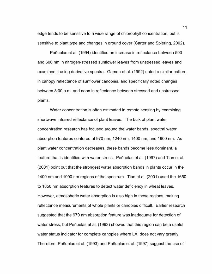
Peñuelas et al. (1994) identified an increase in reflectance between 500
and 600 nm in nitrogen-stressed sunflower leaves from unstressed leaves and
examined it using derivative spectra. Gamon et al. (1992) noted a similar pattern
in canopy reflectance of sunflower canopies, and specifically noted changes
between 8:00 a.m. and noon in reflectance between stressed and unstressed
plants.
Water concentration is often estimated in remote sensing by examining
shortwave infrared reflectance of plant leaves. The bulk of plant water
concentration research has focused around the water bands, spectral water
absorption features centered at 970 nm, 1240 nm, 1400 nm, and 1900 nm. As
plant water concentration decreases, these bands become less dominant, a
feature that is identified with water stress. Peñuelas et al. (1997) and Tian et al.
(2001) point out that the strongest water absorption bands in plants occur in the
1400 nm and 1900 nm regions of the spectrum. Tian et al. (2001) used the 1650
to 1850 nm absorption features to detect water deficiency in wheat leaves.
However, atmospheric water absorption is also high in these regions, making
reflectance measurements of whole plants or canopies difficult. Earlier research
suggested that the 970 nm absorption feature was inadequate for detection of
water stress, but Peñuelas et al. (1993) showed that this region can be a useful
water status indicator for complete canopies where LAI does not vary greatly.
Therefore, Peñuelas et al. (1993) and Peñuelas et al. (1997) suggest the use of

12the ratio of reflectance at 970 nm (Figure 1) to that of a non-water absorbing
region to detect plant water status.
Growth Stage and Canopy Geometry
Reflectance is influenced by the geometric structure (leaf angle) of plant
canopies (Ahlrichs and Bauer, 1982; Demetriades-Shah et al., 1990). Plant
structure changes during the growing season, so growth stage is an important
factor in plant reflectance. Baret et al. (1987) noted that the general behavior of
wheat canopy spectra over a growing season was independent of planting date
and cultivar, but strongly dependent on the growth stage of the plants. Ahlrichs
and Bauer (1982) found the highest correlations of spectral data with plant
parameters between the initiation of tillering and anthesis. They reported good
correlations between reflectance and five plant parameters: percent soil cover,
leaf area index, fresh biomass, dry biomass, and plant water content.
Thenkabail et al. (2002) studied broadband and narrowband spectral
indices and reported that NIR crop reflectance between 750 and 950 nm
changes from flat to upward sloping as plants senesce. They also found a
steeper slope of reflectance between 750 and 950 nm for erectophile plants than
for planophile plants. However, the authors did not elaborate on the cause of
these slopes.
Sensor angle
The effect of sensor angle on reflectance has been recognized for many
years. For instance, Woolley (1971) reported changes in leaf reflectance
13between 400 and 2500 nm based on sensor angle. Woolley showed that
absolute reflectance increased as sensor angle changed from straight-on, and
that reflectance properties change based on whether they are performed on the
abaxial or adaxial leaf surface. Pinter et al. (1987) also observed that spectral
band ratios were significantly affected by off-nadir viewing, and that the NIR/Red
ratio was highest when the sensor was pointed toward a canopy ‘hotspot’
(pointing west in the morning and east in the afternoon) and lowest when the
sensor was pointed away. According to Otterman et al. (1995), vegetated terrain
exhibits strong forward and backscattering.
Solar angle and time of day
Diurnal reflectance measurements of wheat canopies over the visible and
NIR regions of the spectrum suggest that visible reflectance remains roughly
constant throughout the day and infrared reflectance increases as angle from
solar azimuth increases. Asrar et al. (1985) observed that increased solar zenith
angle generally increased LAI estimates that used red and infrared spectral
indices, due to the increase in the infrared. Pinter et al. (1987) reported that
changes in solar angles significantly impacted the NIR/red ratio of winter wheat.
They found that maxima in the NIR/red ratio were attained mid-morning and mid-
afternoon, and minima coincided with the high solar position near midday.
Rahman et al. (1999) also observed that reflectance amplitude varied with sensor
angle in relation to solar angle. Spectral studies are often performed near the

14solar zenith to decrease the effects of solar angle on canopy reflectance
(Osborne et al., 2002; Otterman et al., 1995; Serrano et al., 2000).
Solar position may also influence plant reflectance by influencing the
quantity of light that is incident to the plant. Gamon et al. (1992) suggested that
the xanthophyll chemical changes due to changes in light intensity are partly
responsible for changes in absorption efficiency and changes in leaf reflectance
between morning and afternoon.
Ground cover and the soil background
A significant issue in whole-canopy reflectance experiments is the
variation between green plant cover and the soil background. During early
stages of growth, the soil constitutes a large portion of canopy reflectance. The
primary variable in soil reflectance is brightness, because nearly all spectral data
for a soil falls along a line extending from the origin (Kauth and Thomas, 1976).
High reflecting, light-colored soils influence indices more than do dark, low-
reflecting soils (Jackson et al., 1983). Spectral differences between soils may be
attributed to variations in surface moisture, particle size distribution, soil
mineralogy, soil structure, surface roughness, crusting and presence of shadow
(Huete et al., 1984; Huete et al., 1985). Many reflectance indices are sensitive to
ground cover because ground cover affects red and NIR reflectance.
Jackson et al. (1983) stated that the change in soil reflectance ratios
changes little due to wetting, following the fact that a change in soil reflectance
due to water concentration is about the same in the visible and near-infrared

15(NIR) regions of the spectrum. They also stated that since vegetation reflectance
is very different from soil reflectance, the ratio of red and NIR reflectance is
theoretically a good discriminator of vegetation. Jackson et al. (1983) concluded
that the ratio is not a good discriminator for green vegetation covers less than
50%, but becomes a very sensitive indicator as the ground cover increases.
CURRENT SATELLITE CAPABILITIES
Several commercial and governmental groups sponsor satellite imaging,
and recently launched satellites offer high spatial resolution, several bands, and
rapid return time (Table 2). These characteristics allow a transition between
ground-based imagery and satellite data.
Table 2. Current and planned satellites with features pertinent to reflectance measurements (adapted from Dyke, 2002).
Satellite Launch Pixel Size Bands Return time
ORBView-3 2000 1 m Pan 4 m MSS MSS 4 bands Pan 1 band ±45° off nadir <3 days QuickBird 1999 1 m Pan 3.5 m
MSS Pan 450-900 nm MSS – VNIR 1-5 days
IKONOS 1999 1 m Pan 4 m MSS MSS 4 bands Pan 1 band ALOS 2002 2.5m MSS Channel 1: 0.42 - 0.50 µm
Channel 2: 0.52 - 0.60 µm Channel 3: 0.61 - 0.69 µm Channel 4: 0.76 - 0.89 µm
IRS-P5 1999 2.5m Pan Stereo NEMO 2002 5m Pan 30 m HIS 210 bands 400-2500 nm @10 nm PAN
0.5-0.7µm ORASIS - real-time processing 7 day repeat 2.5 day global average
EO-1 1999 30 m 220 bands 0.4 to 2.5 µm @10nm Grating Imaging Spec
Landsat 7 1999 15 m Pan 30 m MSS 60 mTIR
7 Bands MSS VNIR-TIR 16 days

16SPECTRAL INDICES
Vegetation indices attempt to maximize the spectral contribution from
green vegetation and minimize the effects of soil background and other factors
(Huete et al., 1985; Major et al., 1990). Spectral reflectance has been correlated
with plant health and several leaf biochemical concentrations (Curran, 1989;
Curran et al., 2001). Many reflectance studies use spectral vegetation indices to
determine these parameters.
Spectral indices have been derived for both single-leaf and plant canopy
reflectance measurements. Single-leaf measurements offer the advantage of
higher signal-to-noise ratio and more control over the operating environment,
while canopy measurements allow measurements over a broader scale. Leaf-
scale experiments have ranged from in vivo reflectance of dry plant tissue to
measure leaf biochemical concentrations (Curran et al., 2001) to in situ
chlorophyll concentration determination of intact leaves (Carter and Spiering,
2002). Plant canopy reflectance is also analyzed for green cover and chlorophyll
concentration from both ground and satellite level (Dawson, 2000; Demetriades-
Shah et al., 1990). Studies of both single leaf data (Peñuelas et al., 1993;
Peñuelas et al., 1994) and plant canopy data (Gao, 1996; Peñuelas et al., 1997)
suggest the use of infrared water absorbing bands to detect water stress.
Spectral indicators of crop growth include individual band reflectance
factors, linear combinations of bands by multiple regression, orthogonal
“greenness,” and ratios of infrared and red bands (Dusek et al., 1985). Sims and

17Gamon (2002) suggest that multiple bands are useful because of changes in
absorbance of confounding pigments, such as carotenoids. Best and Harlan
(1985) reported that leaf area estimates using several bands correlated
somewhat more closely with LAI than leaf area estimates using two bands (r2 =
0.73 vs. r2 = 0.69), although Fernández et al. (1994) concluded that NDVI
appears to be the most powerful spectral index that correlates canopy
reflectance with leaf area in winter wheat.
Narrowband spectroradiometers are commonly used for ground-based
and aerial imaging platforms, while satellites with spatial imaging capabilities
sufficient to measure cropland generally employ broadband spectroradiometers.
Baret et al. (1987) noted that although high spectral resolution data correlate well
with classical broadband information, the relationship appears to be dependent
on the phenological stage of the crop. They also stated that a spectral resolution
of about 5 nm appears to be sufficient to show the detail of narrow spectral
properties. Narrowband spectral indices measure slope (Demetriades-Shah et
al., 1990; Peñuelas et al., 1994), shape (Tian et al., 2001), and depth (Curran et
al., 2001; Kokaly and Clark, 1999) of absorption bands, while broadband indices
are limited to measuring the depth.
Ratio and Difference Vegetation Indices
Ratio indices of reflected and transmitted radiation have been used since
the late 1960s to estimate plant growth. Jordan (1969) first published on the use
of the simple ratio vegetation index (RVI), in which he used the ratio of

18transmitted radiation at 800 nm to 675 nm to estimate the leaf area index of a
forest.
Rouse et al. (1973) introduced a variation of the RVI, in which the authors
normalized the reflectance ratio to account for solar angle. This index, later
known as the normalized difference vegetation index (NDVI), includes the NIR
and red reflectance in both the numerator and the denominator. Other
researchers have used a variation of NDVI called green NDVI, or GNDVI to
account for variations in green reflectance instead of red reflectance (Gitelson
and Merzlyak, 1997). NDVI and RVI are the most common vegetation indices
used in remote sensing today.
Soil-Adjusted Vegetation Indices
One approach to dealing with the soil background is to try to eliminate it
using indices that correct for the “soil line.” An early attempt to correct for the soil
line was introduced by Kauth and Thomas (1976), and is referred to as the
perpendicular vegetation index (PVI). The PVI estimates soil brightness by
supplying a soil slope (a) and an offset (b) derived from the NIR vs. red soil
baseline.
The soil-adjusted vegetation index (SAVI) simplifies the soil relationship to
canopy reflectance by adding a simple brightness factor (L), which is typically set
to 0.5, but can range from 0 to 1 (Elvidge and Chen, 1995; Huete, 1988). This
allows a robust estimate of ground cover, although an exact brightness
coefficient is difficult to determine.

19Derivative Indices
One novel narrowband reflectance technique minimizes soil background
effects on canopy spectral signatures by the use of high-resolution derivative
spectra (Demetriades-Shah et al., 1990; Elvidge and Chen, 1995; Hall et al.,
1990; Peñuelas et al., 1994). This allows the discrimination of plant spectra from
the soil background (Figure 2).
The use of derivatives is not new; analytical chemists have used
derivatives to remove background noise for decades. Martin (1957) addressed
the use of both first order and second order derivatives to decrease background
interference. Savitzky and Golay introduced a method for smoothing spectral
data for derivative analysis in 1964 that is still commonly used. However, the
usefulness of derivative spectra was not recognized in plant spectra was not fully
realized until the 1980s (Demetriades-Shah et al., 1990; Hall et al., 1990).
Spectral derivatives can be used for both single-leaf and whole-plant
spectral analysis. Demetriades-Shah et al. (1990) demonstrated that derivative
spectra could yield spectral indices that were superior to conventional broad-
band spectral indices for their studies of plant canopies, and Peñuelas et al.
(1994) separated healthy, water-stressed, and nitrogen-stressed sunflower
leaves based on spectral derivatives. Derivatives eliminate most of the soil
background noise from plant canopy spectral data by normalizing the slope of the
composite plant-soil reflectance spectrum.

20
W ave leng th (nm )400 450 500 550 600 650 700 750 800 850
2nd
Ord
er D
eriv
ativ
e
-4e -5
-3e -5
-2e -5
-1e -5
0
1e-5
2e-5
3e-5
Ref
lect
ance
0 .0
0 .1
0 .2
0 .3
0 .4
0 .5
W h eat
S o il
1st O
rder
Der
ivat
ive
0 .000
0 .001
0 .002
0 .003
Figure 2. Using the linear nature of soil reflectance to eliminate soil background signal using derivatives of reflectance spectra (adapted from Demetriades-Shah et al., 1990).

21Elvidge and Chen (1995) used integrated spectral derivative vegetation
indices with a soil baseline to estimate leaf area index and percent green cover in
a pinyon pine canopy with five different gravel backgrounds. Integrated
derivatives, or antiderivatives, are related to derivative spectra by the
fundamental theorem of calculus (Equation 2).
∫ −=2
1
)()()( 21
λ
λλλ RRdxxr [2]
This theorem states that the sum of the instantaneous changes is a
quantity equal to the overall change of the quantity. Therefore, the integrated
derivative between two wavelengths is the value at the second wavelength minus
the value at the first wavelength, and the integrated derivative index is analogous
to the difference vegetation index (DVI). A baseline correction improves ground
cover estimates over a variety of soil backgrounds, because it dampens the
effects of the soil slope. Derivatives can also be analyzed by the shape,
placement, and height of their peaks to extract information about plant health
(Peñuelas et al., 1994), although these characteristics can change between leaf
and canopy level measurements.
Elvidge and Chen (1995) tested derivative green cover estimates using
both first- and second-order derivative indices (Figure 3). The first-order
derivative index was normalized to the spectral slope at 626 nm. The authors
observed that a first-order derivative green vegetation index integrated between
626 and 795 nm with a local baseline provided the most linear relationships to
LAI and percent green cover over several soil backgrounds (r2 = 0.945), closely

22followed by the second derivative green vegetation index. These derivative
indices were found to be superior to PVI and SAVI at estimating ground cover
and LAI (Figure 4). Without the local baseline, first derivative correlations were
substantially poorer than second-derivative correlations.
The first-order analysis is essentially an application of the simple DVI, with
a correction for the slope of the soil background added through the local
baseline. The second-order derivative analysis did not show substantial
improvement using this correction method because of its inherent ability to
eliminate the soil slope.
Figure 3. Use of a local baseline with 1st order derivative spectra to eliminate soil background signal. This idea was first published by Elvidge and Chen (1995).

23
Bro
ad B
and
ND
VI
0.00
0.10
0.20
0.30
0.40
0.50
0.60WhiteGreyBrownBlackRed
Nar
row
Ban
d S
AV
I
0.00
0.02
0.04
0.06
0.08
0.10
0.12
0.14
Leaf Area Index0.00 0.05 0.10 0.15 0.20 0.25 0.30 0.35
Der
ivat
ive-
Base
d (D
GV
I)
0.00
0.02
0.04
0.06
0.08
0.10
r2 = 0.39
r2 = 0.85
r2 = 0.94
Figure 4. Comparison of derivative green cover estimates with common non-derivative vegetation indices to estimate LAI with different background colors (adapted from Elvidge and Chen, 1995).
24Another application of derivative analysis has been proposed by Adams et
al. (1999) as a method for determining chlorophyll concentration. The
yellowness index is a three-point approximation of the second derivative between
550 and 650 nm and has shown positive results in identifying the chlorophyll
concentration of manganese-deficient soybean plants.
The premise of the yellowness index is that the shape of the green
reflectance spectra changes as plants become chlorotic. A second derivative
analysis of this shape accentuates these changes in shape, allowing the
identification of chlorotic plants based on this change in shape. This method
assumes that all chlorotic plants exhibit this characteristic. The authors noted
that although the 550 to 650 nm range was used for their study, other
wavelengths might be appropriate, depending on the crop species and other
physiological and environmental factors.
Band Depth Analysis
Another method for decreasing background effects is normalized band
depth analysis. Because the absorptions of different plant materials are similar
and overlapping (Table 1), single absorption bands cannot generally be isolated
and directly related to the concentration of a single plant constituent. Therefore,
Kokaly and Clark (1999) proposed the normalization of broad absorption bands
to investigate plant stress. The reflectance signature is first processed through
continuum removal (Clark and Roush, 1984).

25A continuum line is approximated by a linear function that passes over an
absorption feature of interest and connects two points of the reflectance
spectrum that are unaffected by the absorption feature. The band depth is then
calculated by dividing the absorption band reflectance by the continuum line.
The continuum-removed spectrum is then normalized by measuring the depth at
the center of the band and the area under the band depth curve. These
measurements are termed band depth normalized to band depth at the center of
the absorption feature (BNC) and band depth normalized to area of absorption
feature (BNA). The result is an index that is insensitive to spectral contaminants.
This technique was demonstrated to be effective in regions of the spectrum
above 1000 nm.
Curran et al. (2001) found that reflectance analysis performed on dried
and ground slash pine needles using the Kokaly and Clark methodologies
compared favorably with laboratory biochemical assays, and that both BNC and
BNA methods of band normalization resulted statistically more accurate
differences in biochemical concentration estimates than derivative methods.
Furthermore, Clark and Roush (1984) found moderate (r2 ≈ 0.60) to high (r2 >
0.95) levels of accuracy for estimation of twelve foliar biochemicals using band
normalization.
REFERENCES
Adams, M.L., W.D. Philpot, and W.A. Norvell. 1999. Yellowness index: an application of spectral second derivatives to estimate chlorosis of leaves in stressed vegetation. Int. J. Remote Sens. 20:3663-3675.
26Ahlrichs, J.S., and M.E. Bauer. 1982. Relation of agronomic and multispectral
reflectance characteristics of spring wheat canopies. LARS Technical Report 121082:26p. Purdue University, Lafayette, IN.
ASD. 1999. Analytical Spectral Devices, Inc. technical guide. 3rd ed., Boulder, Colorado.
Asrar, G., E.T. Kanemasu, and M. Yoshida. 1985. Estimates of leaf area index from spectral reflectance of wheat under different cultural practices and solar angle. Remote Sens. Environ. 17:1-11.
Baret, F., I. Champion, G. Guyot, and A. Podaire. 1987. Monitoring wheat canopies with a high spectral resolution radiometer. Remote Sens. Environ. 22:367-378.
Best, R.G., and J.C. Harlan. 1985. Spectral estimation of green leaf area index of oats. Remote Sens. Environ. 17:27-36.
Carter, G.A., and B.A. Spiering. 2002. Optical properties of intact leave for estimating chlorophyll concentration. J. Environ. Qual. 31:1424-1432.
Clark, R.N., and T.L. Roush. 1984. Reflectance spectroscopy: quantitative analysis techniques for remote sensing applications. J. Geophys. Res. 89:6329-6340.
Costa, C., L.M. Dwyer, P. Dutilleul, D.W. Stewart, B.L. Ma, and J.D. Smith. 2001. Inter-relationships of applied nitrogen, spad, and yield of leafy and non-leafy maize genotypes. J. Plant Nutr. 24:1173-1194.
Curran, P.J. 1989. Remote sensing of foliar chemistry. Remote Sens. Environ. 30:271-278.
Curran, P.J., J.L. Dungan, and D.L. Peterson. 2001. Estimating the foliar biochemical concentration of leaves with reflectance spectrometry: testing the Kokaly and Clark methodologies. Remote Sens. Environ. 76:349-359.
Dawson, T.P. 2000. The potential for estimating chlorophyll content from a vegetation canopy using the medium resolution imaging spectrometer (MERIS). Int. J. Remote Sens. 21:2043-2051.
Dawson, T.P., and P.J. Curran. 1998. A new technique for interpolating the reflectance red edge position. Int. J. Remote Sens. 19:2133-2139.
Demetriades-Shah, T.H., M.D. Steven, and J.A. Clark. 1990. High resolution derivative spectra in remote sensing. Remote Sens. Environ. 33:55-64.
27Dusek, D.A., R.D. Jackson, and J.T. Musick. 1985. Winter wheat vegetation
indices calculated from combinations of seven spectral bands. Remote Sens. Environ. 18:255-267.
Dyke, A. 2002. Future sensor summary [Online]. Available by Ultraspectral LLC http://www.ultraspectral.com/Future%20Sensor%20Summary.htm (posted February 24, 2002; verified December 23, 2002).
Elvidge, C.D., and Z. Chen. 1995. Comparison of broad-band and narrow-band red and near-infrared vegetation indices. Remote Sens. Environ. 54:38-48.
Fernández, S., D. Vidal, E. Simón, and L. Solé-Sugrañes. 1994. Radiometric characteristics of Triticum aestivum cv. Astral under water and nitrogen stress. Int. J. Remote Sens. 15:1867-1884.
Filella, I., L. Serrano, J. Serra, and J. Penuelas. 1995. Evaluating wheat nitrogen status with canopy reflectance indices and discriminant analysis. Crop Sci. 35:1400-1405.
Gamon, J.A., J. Penuelas, and C.B. Field. 1992. A narrow-waveband spectral index that tracks diurnal changes in photosynthetic efficiency. Remote Sens. Environ. 41:35-44.
Gao, B.-C. 1996. NDWI -- a normalized difference water index for remote sensing of vegetation liquid water from space. Remote Sens. Environ. 58:257-266.
Gates, D.M. 1980. Biophysical ecology. Springer-Verlag, New York.
Gitelson, A.A., and M.N. Merzlyak. 1997. Remote estimation of chlorophyll content in higher plant leaves. Int. J. Remote Sens. 18:2691-2697.
Hall, F.G., K.F. Huemmrich, and S.N. Goward. 1990. Use of narrow-band spectra to estimate the fraction of absorbed photosynthetically active radiation. Remote Sens. Environ. 32:47-54.
Horler, D.N.H., M. Dockray, and J. Barber. 1983a. The red edge of plant leaf reflectance. Int. J. Remote Sens. 4:273-288.
Horler, D.N.H., M. Dockray, J. Barber, and A.R. Barringer. 1983b. Red edge measurements for remotely sensing plant chlorophyll content. Adv. Space Res. 3:273-277.

28Huete, A.R. 1988. A soil-adjusted vegetation index (SAVI). Remote Sens.
Environ. 25:295-309.
Huete, A.R., D.F. Post, and R.D. Jackson. 1984. Soil spectral effects on 4-space vegetation discrimination. Remote Sens. Environ. 15:155-165.
Huete, A.R., R.D. Jackson, and D.F. Post. 1985. Spectral response of a plant canopy with different soil backgrounds. Remote Sens. Environ. 17:37-53.
Jackson, R.D., P.N. Slater, and P.J. Pinter. 1983. Discrimination of growth and water stress in wheat by various vegetation indices through clear and turbid atmospheres. Remote Sens. Environ. 13:187-208.
Jago, R.A., M.E.J. Cutler, and P.J. Curran. 1999. Estimating canopy chlorophyll concentration from field and airborne spectra. Remote Sens. Environ. 68:217-224.
Jones, M.J. 1997. Organic chemistry. W.W. Norton and Company, New York.
Jordan, C.F. 1969. Derivation of leaf area index from quality of light on the forest floor. Ecology 50:663-666.
Kauth, R.J., and G.S. Thomas. 1976. The tasseled cap -- A graphic description of the spectral-temporal development of agricultural crops as seen by Landsat. Proceedings of the Symposium on Machine Processing of Remotely Sensed Data:41-51.
Kokaly, R.F., and R.N. Clark. 1999. Spectroscopic determination of leaf biochemistry using band-depth analysis of absorption features and stepwise multiple linear regression. Remote Sens. Environ. 67:267-287.
Major, D.J., F. Baret, and G. Guyot. 1990. A ratio vegetation index adjusted for soil brightness. Int. J. Remote Sens. 11:727-740.
Martin, A.E. 1957. Difference and derivative spectra. Nature 180:231-233.
Monje, O., and B. Bugbee. 1992. Inherent limitations of nondestructive chlorophyll meters: a comparison of two types of meters. HortScience 27:69-71.
Osborne, S.L., J.S. Schepers, D.D. Francis, and M.R. Schlemmer. 2002. Use of spectral radiance to estimate in-season biomass and grain yield in nitrogen- and water-stressed corn. Crop Sci. 42:165-171.

29Otterman, J., T. Brakke, and J. Smith. 1995. Effects of leaf-transmittance versus
leaf-reflectance on bi-directional scattering from canopy/soil surface: an analytical study. Remote Sens. Environ. 54:49-60.
Peñuelas, J., I. Filella, C. Beil, L. Serrano, and R. Savé. 1993. The reflectance at the 950-970 nm region as an indicator of plant water status. Int. J. Remote Sens. 14:1887-1905.
Peñuelas, J., J.A. Gamon, A.L. Fredeen, J. Merino, and C.B. Field. 1994. Reflectance indices associated with physiological changes in nitrogen- and water-limited sunflower leaves. Remote Sens. Environ. 48:135-146.
Peñuelas, J., J. Piñol, R. Ogaya, and I. Filella. 1997. Estimation of plant water concentration by the reflectance water index WI (R900/R970). Int. J. Remote Sens. 18:2869-2875.
Pinter, P.J., G. Zipoli, G. Maracchi, and R.J. Reginato. 1987. Influence of topography and sensor view angles on NIR/red ratio and greenness vegetation indices of wheat. Int. J. Remote Sens. 8:953-957.
Porra, R.J., W.A. Thompson, and P.E. Kriedemann. 1989. Determination of accurate extinction coefficients and simultaneous equations for assaying chlorophylls a and b extracted with four different solvents: verification of the concentration of chlorophyll standards by atomic absorption spectroscopy. Biochim. Biophys. Acta. 975:384-394.
Rabideau, G.S., C.S. French, and A.S. Holt. 1946. The absorption and reflection spectra of leaves, chloroplast suspensions, and chloroplast fragments as measured in an Ulbricht Sphere. Am. J. Bot. 33:769-777.
Rahman, H., D.A. Quadir, A.Z.M.Z. Islam, and S. Dutta. 1999. Wiewing angle effect on the remote sensing monitoring of wheat and rice crops. Geocarto International 14:75-79.
Rouse, J.W., R.H. Haas, J.A. Schell, and D.W. Deering. 1973. Monitoring vegetation systems in the great plains with ERTS, p. 309-317. Third ERTS Symposium, NASA SP-351, Vol. 1. NASA, Washington, DC.
Savitzky, A., and M.J.E. Golay. 1964. Smoothing and differentiation of data by simplified least squares procedures. Anal. Chem. 36:1627-1639.
Serrano, L., I. Filella, and J. Penuelas. 2000. Remote sensing of biomass and yield of winter wheat under different nitrogen supplies. Crop Sci. 40:723-731.
30Sims, D.A., and J.A. Gamon. 2002. Relationships between leaf pigment content
and spectral reflectance across a wide range of species, leaf structures and developmental stages. Remote Sens. Environ. 81:337-354.
Taiz, L., and E. Zeiger. 2002. Plant physiology. 2nd ed. Sinauer Associates, Sunderland, MA.
Thenkabail, P.S., R.B. Smith, and E.D. Pauw. 2002. Evaluation of narrowband and broadband vegetation indices for determining optimal hyperspectral wavebands for agricultural crop characterization. Photogramm. Eng. Remote Sens. 68:607-621.
Tian, Q., C. Zhao, Q. Tong, R. Pu, and X. Guo. 2001. Spectroscopic determination of wheat water status using 1650-1850 nm spectral absorption features. Int. J. Remote Sens. 22:2329-2338.
Weidner, V.R., and H.H. Hsia. 1981. Reflection properties of pressed polytetrafluoroethylene powder. J. Optical Soc. Am. 71:856-861.
Woolley, J.T. 1971. Reflectance and transmittance of light by leaves. Plant Physiol. 47:656-662.

31CHAPTER 3
DEVELOPMENT OF A NOVEL SPECTRAL REFLECTIVE INDEX TO
DIFFERENTIATE NITROGEN AND WATER STRESS
FROM EMERGENCE TO CANOPY CLOSURE
ABSTRACT
Spectral reflectance of plant canopies provides an accurate indication of
ground cover fraction, which is highly correlated with radiation capture. If
nutrients and water do not limit growth, radiation capture is highly correlated with
daily growth rate and ultimate yield. However, if nutrients and water limit growth,
none of the common spectral indices are able to separate a more developed,
stressed canopy from a less-developed, rapidly growing canopy. We have long
known that nitrogen stress is highly correlated with reduced chlorophyll
concentration and increased reflectance of green radiation. Conversely, water
stress inhibits leaf expansion, which increases chlorophyll concentration and
decreases green reflectance. In a two-year study, we measured ground-based
canopy reflectance of wheat plots in nitrogen and water stressed environments
and found that all of the common spectral indices were highly correlated with
ground cover fraction, but none of them could distinguish the intensity of leaf
color from ground cover fraction. Here we report a reflective index that can
differentiate nitrogen and water stress over a wide range of ground cover. The
index is based on the ratio of the green and red variants of the normalized
difference vegetation index (NDVIgreen/NDVIred). The new index was able to

32distinguish N and water stress from satellite data using wavelengths less than
1000 nm. This index should be broadly applicable over a wide range of plant
types and environments.
INTRODUCTION
Reflectance of red and green radiation by plants is heavily influenced by
chlorophyll absorption. Past studies of reflective leaf biochemicals have
emphasized that the photosynthetic pigment chlorophyll dominates visible and
near-infrared leaf reflectance and forms the basis for most reflectance estimates
of plant health (Curran, 1989). Chlorophyll concentration is closely correlated
with changes in visible and near-infrared reflectance, so ratios of reflectance at
chlorophyll-sensitive and chlorophyll-insensitive wavelengths are often used to
determine chlorophyll concentration.
Red is the most widely used chlorophyll-sensitive spectral region. Red
reflectance is sensitive to very low chlorophyll concentrations, making it ideal to
estimate ground cover. However, red reflectance saturates at moderate
chlorophyll levels, making it insensitive to higher levels of chlorophyll content.
The red edge is another chlorophyll-sensitive spectral region. The red
edge, as described by Horler et al. (1983), is the area of sharp change in leaf
reflectance between the red and near-infrared spectral domains. The red edge
tends to be sensitive to a wide range of chlorophyll concentration, but is also
affected by plant type and changes in ground cover (Carter and Spiering, 2002).

33Green reflectance is also sensitive to a wider range of chlorophyll
concentration than is red reflectance and is broader, flatter, and less sensitive
than the red edge to variation of plant type and changes in ground cover.
Therefore, at moderate to high chlorophyll levels, red reflectance remains
generally constant, but green reflectance continues to decrease with increasing
chlorophyll concentration (Gitelson and Merzlyak, 1997).
Nitrogen and water availability both affect the chlorophyll concentration of
plant leaves. Nitrogen is an integral part of the chlorophyll molecule (Taiz and
Zeiger, 2002), and nitrogen stress decreases chlorophyll concentration (Yoder
and Pettigrew-Crosby, 1995). Water stress, on the other hand, does not directly
affect chlorophyll synthesis, but rather decreases leaf area. Because the leaf
area decreases and the amount of chlorophyll does not change, the net effect is
an increase of leaf chlorophyll concentration (Peñuelas et al., 1994). Fernández
et al. (1994) noted that unirrigated wheat plants were also more erectophile than
irrigated plants in their study. They found that this characteristic affected plant
reflectance in two ways. First, the vertical elements of an erectophile canopy
would trap larger quantities of radiation than a planophile canopy, resulting in a
decrease of reflected radiation from the canopy to the sensor. Second, the
erectophile leaves would increase leaf area index for a given ground cover
fraction, resulting in a higher leaf chlorophyll density per unit ground area. This
would also result in an apparent increase in chlorophyll concentration as sensed
by a spectrometer. These findings are consistent with the findings of Jackson
and Pinter (1986).
34Methods for Estimating Ground Cover
Many studies have determined ground cover fraction and chlorophyll per
unit ground area using spectral indices. These indices maximize the spectral
contribution from green vegetation and minimize background effects, such as soil
reflectance (Huete et al., 1985; Major et al., 1990). Most of these indices can be
used to estimate ground cover (the percent of soil covered by plants in a given
area) or leaf area index (LAI; the ratio of leaf area to ground area).
Vegetation indices detect ground cover based on the sharp spectral
changes that occur as vegetation covers the soil. Soil reflectance slopes
gradually upward through the visible and near-infrared. Vegetation, however, is
heavily influenced by chlorophyll absorption, and reflects more green and near-
infrared radiation than red radiation. Vegetation fraction is identifiable through
changes in visible and near-infrared reflectance, and ratios of red and near-
infrared radiation typically correlate closely with ground cover.
Table 3 lists the common spectral indices that estimate ground cover and
correct for contaminating spectral influences. The simplest vegetation indices
use simple ratios or differences between two spectral regions to estimate growth.
The two simplest indices are called the ratio vegetation index (RVI) and the
difference vegetation index (DVI). The RVI is usually determined as the ratio of
near-infrared reflectance to red reflectance, although researchers have used
ratios of other bands as well to determine plant health (e.g. Peñuelas et al.,
1997).. The DVI is determined as the simple difference between two

35wavelengths. Rouse et al. (1973) introduced a normalized variation of the RVI,
which was later called the normalized difference vegetation index (NDVI). The
NDVI is widely used to estimate fractional ground cover over a wide range of light
intensity.
Table 3. Broad-band and narrow-band vegetation indices that are widely used for ground cover determination. These indices are based on the differential absorption of green, red, and near-infrared radiation by plant chlorophyll. The indices are arranged from oldest to newest.
Abbreviation Name Vegetation Index Reference RVI Ratio Vegetation Index
REDNIRRVI =
(Jordan, 1969)
NDVIred Normalized Difference Vegetation Index
( )( )REDNIR
REDNIRNDVI+−
= (Rouse et al., 1973)
PVI Perpendicular Vegetation Index
21 abaREDNIRPVI
+
−−=
(Richardson and Weigand, 1977)
DVI Difference Vegetation Index
REDNIRDVI −= (Tucker, 1979)
SAVI Soil Adjusted Vegetation Index )1(
)()( LLREDNIR
REDNIRSAVI +++
−=
(Huete, 1988)
1DL_DGVI First-order derivative green vegetation index using local baseline
( ) ( ) ii
n
DGVIDL λλρλρλ
λ
∆−= ∑1
1''_1
(Elvidge and Chen, 1995)
1DZ_DGVI First-order derivative green vegetation index using zero baseline
( ) ii
n
DGVIDZ λλρλ
λ
∆= ∑1
'_1 (Elvidge and Chen, 1995)
2DZ_DGVI Second-order derivative green vegetation index
( ) ii
n
DGVIDZ λλρλ
λ
∆= ∑1
"_2 (Elvidge and Chen, 1995)
NDVIgreen Green Normalized Difference Vegetation Index
( )( )GREENNIR
GREENNIRGNDVI+−
= (Gitelson and Merzlyak, 1998)
YI Yellowness Index ( ) ( ) ( )2
101 2λ
λλλ∆
+−∝ +− RRR
YI (Adams et al., 1999)

36The green NDVI, or NDVIgreen, is analogous to NDVI, except that it
substitutes green reflectance for red reflectance (Gitelson and Merzlyak, 1997).
Unless otherwise specified in this paper, NDVI will refer to the red variation of the
NDVI and will be used to denote the estimate of ground cover by NDVI. The
index will be referred to as NDVIred and NDVIgreen on occasions where the two
variations of this index are compared with each other.
Although the oldest vegetation indices are still widely used, several newer
indices have been developed in an attempt to increase the accuracy of ground
cover estimation.
During early stages of vegetation development and growth, the soil
constitutes a large portion of plant canopy reflectance. To overcome the effects
of soil, some vegetation indices add a correction factor to the basic index that
accounts for soil brightness. An early attempt to correct for soil brightness was
introduced by Kauth and Thomas (1976), and is referred to as the perpendicular
vegetation index (PVI). The PVI assumes that soil reflectance is essentially
linear throughout the visible and near-infrared spectral regions. A slope (a) and
an offset (b) of the soil reflectance are measured, and plant reflectance is
computed as a perpendicular function from the original soil line. Later, Huete
(1988) suggested the application of a soil-adjusted vegetation index (SAVI) to
account for soil brightness. The L value in the SAVI equation is a brightness
coefficient that accounts for soil color. The L value can be set between zero
(black soil) and one (white soil). The estimate of a soil brightness coefficient is
37difficult to ascertain, as alluded to by the authors, and is often arbitrarily set to
0.5.
Derivative vegetation indices, such as the first derivative green vegetation
index and the second derivative green vegetation index (Elvidge and Chen,
1995), attempt to eliminate soil reflectance based on its linear nature. Although
derivative indices are analogous in their most basic form to the DVI,
Demetriades-Shah et al. (1990) pointed out that first- and second-derivative
indices can essentially eliminate soil signal. Derivative indices were found by
Elvidge and Chen (1995) to be superior to ratio indices in determining plant
ground cover over a variety of backgrounds during their tests (see Appendix 3).
The estimate of plant ground cover in itself, however, is not an estimate of
plant health. Although canopy reflectance indices have been correlated to
nitrogen status (Fernández et al., 1994; Hinzman et al., 1986) and water status
(Jackson et al., 1983), these parameters are estimated on a ground area basis,
and the indices do not differentiate between leaf color and ground cover (Adams
et al., 1999).
Spectral Indicators of Plant Color
As referenced earlier, the heavy influence of plant ground cover on
canopy reflectance allows vegetation indices to estimate ground cover, but
complicates the analysis of chlorophyll and nitrogen concentration, especially for
incomplete crop canopies. Demetriades-Shah et al. (1990) pointed out that
standard spectral vegetation indices are unable to differentiate between low plant

38cover and decreases in plant health. In the past, several researchers have
avoided the ground cover issue by correlating canopy reflectance with chlorophyll
density on a soil area basis (e.g. Hinzman et al., 1986). Unfortunately, this
method does not give any indication of leaf chlorophyll concentration separate
from ground cover.
Demetriades-Shah and Court (1987) discussed the shortcoming of
vegetation indices to estimate chlorophyll concentration and suggested the use
of oblique (low angle) reflectance measurements to maximize the vegetation
reflectance within the field-of-view and minimize the contribution of the soil
reflectance to the overall reflectance measurement. Most spectral
measurements are made with the sensor facing perpendicular to the soil surface,
but oblique measurements are made with the sensor nonperpendicular to the
surface. Demetriades-Shah and Court (1987) used this method to separate
nitrogen-stressed from unstressed canopies using NDVI. However, Pinter et al.
(1987) observed that oblique measurements significantly affect the ratios of red
and near-infrared reflectance, and Otterman et al. (1995) noted that the
reflectance of vegetated terrain is influenced heavily by the bidirectional
scattering of solar radiation by plants. Changes in solar angle make oblique
measurements difficult to replicate, and oblique readings do not allow the
measurement of ground cover and plant color at the same time. Oblique
measurements also cannot be scaled directly from ground-based to satellite
measurements.

39Other studies have attempted to identify stress by comparing spectral
bands. Fernández et al. (1994) attempted to resolve plant nitrogen status by
making a linear correlation between wheat nitrogen status and plant reflectance
of red and green radiation. However, both red reflectance and green reflectance
are affected by ground cover, and the authors did not explain how this linear
correlation eliminates the ground cover issue from their estimate. Osborne et al.
(2002) compared similar linear combinations of green, red, and near-infrared
reflectance to determine nitrogen status in corn. However, they did not report a
method to correct for ground cover, and the reported relationship between their
coefficients of reflectance and plant nitrogen concentration was dependent on the
sampling date.
Another suggested solution to the challenge of separating ground cover
from plant greenness has been the use of derivative analysis of reflectance
spectra to identify plant stress independently of ground cover. Demetriades-
Shah et al. (1990) demonstrated the use of derivative spectra to suppress low-
frequency background noise associated with soil reflectance, resulting in
derivative spectral indices that identified plant chlorosis based on spectral shifts
in the reflectance between healthy and chlorotic plants. Derivative analysis
eliminates the effects of soil reflectance, which is characteristically linear
throughout the visible and near-infrared spectral regions. However, derivatives
introduce new complexity into spectral estimates, increase low-level noise, and
may still need to be normalized to correct for soil characteristics (Elvidge and
Chen, 1995). It is notable that integrated first-derivative indices are analogous to

40the difference vegetation index over the wavelengths of interest. Derivative
indices are also difficult to use from broad band spectral data, although Adams et
al. (1999) suggested the use of broad band estimates of derivatives as a solution
to this challenge.
Based on this discussion, current vegetation indices are unable to
satisfactorily separate plant color from ground cover. Oblique measurements are
subject to scattering effects and do not provide a ground cover estimate. Linear
comparisons of green and red wavelengths do not address the ground cover
issue, because they do not take into account the changes of reflectance for each
color with changes in ground cover. Derivatives add complexity and high-level
noise.
The combination of the chlorophyll-saturated NDVIred as a ground cover
indicator and the chlorophyll-sensitive NDVIgreen as a plant color indicator has the
potential to separate plant color from the ground cover component of plant
health. Because NDVIred and NDVIgreen are normalized to the same near-infrared
wavelength, the influence of ground cover is minimized.
The focus of this research was to find a method to differentiate plant
chlorosis from ground cover. Therefore, this research consisted of two
objectives. The first objective was to test several vegetation indices to find the
most effective index for detecting vegetation cover so that nitrogen stress
determination could be based on the most robust index. The second was to
evaluate the extent to which nitrogen-stressed plant canopies can be
differentiated from unstressed and water-stressed canopies independent of
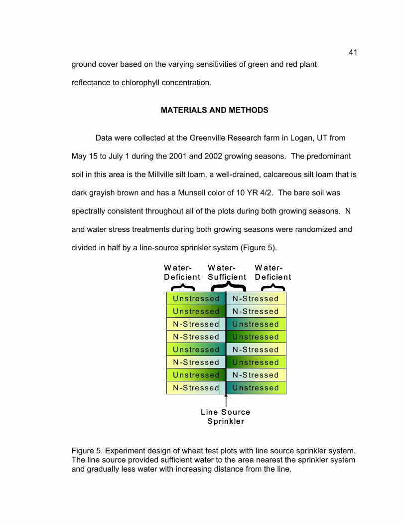
41ground cover based on the varying sensitivities of green and red plant
reflectance to chlorophyll concentration.
MATERIALS AND METHODS
Data were collected at the Greenville Research farm in Logan, UT from
May 15 to July 1 during the 2001 and 2002 growing seasons. The predominant
soil in this area is the Millville silt loam, a well-drained, calcareous silt loam that is
dark grayish brown and has a Munsell color of 10 YR 4/2. The bare soil was
spectrally consistent throughout all of the plots during both growing seasons. N
and water stress treatments during both growing seasons were randomized and
divided in half by a line-source sprinkler system (Figure 5).
U nstressed
U nstressed
N -S tressed
U nstressed
U nstressed
N -S tressed
N -S tressed
U nstressed
N -S tressed
U nstressed
U nstressed
U nstressed
} }W ater-S u ffic ien t
W ate r-D efic ien t
W ater-D e fic ien t
N -S tressed
N -S tressed
N -S tressed
N -S tressed
L ine S ourceS prink le r
U nstressed
U nstressed
N -S tressed
U nstressed
U nstressed
N -S tressed
N -S tressed
U nstressed
N -S tressed
U nstressed
U nstressed
U nstressed
} }W ater-S u ffic ien t
W ate r-D efic ien t
W ater-D e fic ien t
N -S tressed
N -S tressed
N -S tressed
N -S tressed
L ine S ourceS prink le r
Figure 5. Experiment design of wheat test plots with line source sprinkler system. The line source provided sufficient water to the area nearest the sprinkler system and gradually less water with increasing distance from the line.

42
Control plots were initially fertilized with 100 kg ha-1 nitrogen, 110 kg ha-1
phosphorus, and 45 kg ha-1 potassium. Nitrogen-deficient plots were fertilized
with the same phosphorus and potassium, but no nitrogen. A line source
sprinkler system provided a gradated water application from the center outward,
which introduced a gradual addition of water stress. Plots were divided into three
water treatment groups based on proximity to the line source. The half of each
plot closest to the line source received ample water during the growing season
and was used as the control. The outer regions of each plot received 50% and
10% of potential evapotranspiration (ET) based on the application to the inner
plots. Sample points were chosen randomly throughout the plots and provided
five to eight replicate sample points for each treatment. Plots were watered
every three to five days, depending on weather conditions. Irrigation was
measured with water gauges placed along the length of a test strip to verify water
deficit. All measurements were performed when the surface in all treatments
was dry to eliminate the effects of varying soil reflectance between treatments.
Reflectance measurements were made on sunny days from tillering through
anthesis with a field-portable fiber optic spectrometer (Model EPP2000,
StellarNet, Inc., Tampa, FL) with a 2-nm spectral resolution (FWHM) and a
spectral range of 400-950 nm. Each spectral measurement was made with the
sensor suspended 1.5 meters above the surface. Almost all measurements were
made within two hours of solar noon to minimize view angle effects. Spectral
data was smoothed using Savitzky-Golay least squares spectral smoothing over

43a 5 nm range (Savitzky and Golay, 1964). Smoothed data was exported into a
spreadsheet and analyzed. The spectral indices listed in Table 3 were calculated
for each sample plot during the growing season. For the RVI, NDVIred, PVI, DVI,
and SAVI, 675 nm was used as the red reflectance. The NDVIgreen used 550 nm
as the green reflectance. All of the indices used 840 nm as the NIR reflectance.
The derivative vegetation indices were calculated between 626 nm and 795 nm,
as described by Elvidge and Chen (1995). For the yellowness index, reflectance
at 580 nm was used as 8-1, reflectance at 624 nm was used as 80, reflectance at
668 nm was used as 8+1, and ∆8 was 44 nm, as examined by Adams et al.
(1999).
Plant ground cover was measured using a digital camera that was
suspended over each sample point. A large white foam board was used as a
baffle to block direct solar radiation, allowing pictures to be taken on sunny days
without sharp shadows below the plants. This minimized the analysis time for
each picture and increased the accuracy of the ground cover estimate.
Image analysis was performed in Adobe Photoshop (Adobe Systems, Inc.,
San Jose, CA), an off-the-shelf photo-editing program. The soil component was
deleted using the magic wand tool and the magic eraser tool, both of which allow
the selection of pixels with similar colors. Ground cover was then calculated for
each image using the histogram function, with green pixels calculated as the
fraction of total pixels. Previous studies in our laboratory using this technique
have indicated that these digital images of ground cover were highly correlated

44with radiation capture (r2 = 0.995) and canopy photosynthesis (r2 = 0.998)
(Klassen et al., 2003).
Leaf chlorophyll concentration was measured with a chlorophyll meter
(SPAD-502, Minolta, Ramsey, NJ), and the chlorophyll measurements were used
as a basis for comparison with the spectrometer. The SPAD-502 chlorophyll
meter is a dual-wavelength meter that emits light from a red LED and an infrared
LED in sequence through a leaf to measure leaf absorbance. Peak chlorophyll
absorbance is measured at 650 nm, and nonchlorophyll absorbance is measured
at 940 nm by sensors inside the instrument (Monje and Bugbee, 1992). The
meter output value is based on the ratio of transmittance at these wavelengths
and ranges from about 15 (highly chlorotic) to 60 (dark green) for Westbred 936
spring wheat. Ten SPAD chlorophyll readings of separate plants were made on
at each sample site and averaged to estimate the chlorophyll concentration of the
plants at the site. All measurements were performed on the top unfolded leaf of
each plant.
After the derivation of our method, a 2002 IKONOS satellite image of a
production Westbred 936 spring what field at Minidoka, Idaho. The soil at this
site was generally uniform and consisted of alluvial and loess deposits of silt
loam. Most of the soil in the region is Minidoka silt loam, a coarse-silty, mixed
superactive, mesic Xerollic Durorthid with a color of 10YR 6/3, 10YR 4/2 moist.
The Idaho plots consisted two replicates of four treatments: 0, 60, 150, and 195
kg ha-1 applied nitrogen. The nitrogen application of the control study was 150

45kg ha-1 pre-plant. Plant cover at the time of the image ranged from 50 to almost
100%, depending upon the treatment.
RESULTS
Comparison of Indices to Measure Ground Cover
All but one of the 10 common spectral indices accurately determined
ground cover (as determined from digital images) throughout the growing season
(Table 4). The ratio vegetation indices (RVI, NDVIred, NDVIgreen, PVI, and SAVI)
had a higher coefficient of determination of ground cover than the difference or
derivative indices (Appendix 6). The ratio indices were more consistent than the
simple difference indices, because the ratio of reflectance between wavelengths
is more constant than differences of reflectance between wavelengths.
Indices that corrected for soil brightness did not improve the prediction of
ground cover for this study, because the soil was spectrally similar throughout
the test site.
The yellowness index (YI) was poorly correlated with ground cover,
probably because the YI was designed to derive plant yellowness and not ground
cover. Digital ground cover estimates and NDVI were well correlated with plant
growth during the growing season (Figure 6). Although the average plot NDVI
varied among sampling dates during the growing season, it followed plant growth
and allowed a full-season estimate of ground cover and final yield (Appendix 1).

46Table 4. Comparison of ratio and difference vegetation indices with digital images of ground cover collected during the entire growing season. Ratio indices were better correlated with ground cover than difference indices. The yellowness index had a poor correlation with ground cover.
Index Class
Name Coefficient of Determination (r2) with Ground Cover
Ratio Ratio Vegetation Index (RVI) 0.88 Normalized Difference Vegetation Index (NDVI) 0.88 Perpendicular Vegetation Index (PVI) 0.87 Soil Adjusted Vegetation Index (SAVI) 0.90 Green Normalized Difference Vegetation Index
(NDVIgreen) 0.90
Difference Difference Vegetation Index (DVI) 0.82 Derivative First-order derivative green vegetation index
using local baseline (1DL_DGVI) 0.83
First-order derivative green vegetation index using zero baseline (1DZ_DGVI)
0.82
Second-order derivative green vegetation index (2DZ_DGVI)
0.73
Yellowness Index (YI) 0.28
Days After Planting0 20 40 60 80
ND
VI re
d
0.0
0.2
0.4
0.6
0.8
1.0
Gro
und
Cov
er (%
)
0
20
40
60
80
100
Digital Image r2 = 0.98
NDVIred2002
Figure 6. Comparison of NDVI with ground cover (measured by a digital camera) over time. Digital images and NDVI increased in a similar manner during the growing season based on plant growth.

47
Differentiating N and Water Stress
Although stressed treatments were easily differentiated from unstressed
treatments during both growing seasons based on NDVI (Figure 7), the close
relationship between NDVI and ground cover indicated that most of this
separation was due to changes in ground cover. Water-stressed and nitrogen-
stressed plots were almost identical during the 2001 growing season (Figure 7).
This similarity emphasizes the confounding effects of ground cover, since water
and nitrogen stress could not be separated by NDVI, even though the chlorophyll
concentration in water-stressed and nitrogen-stressed leaves was quite different.
Days After Planting35 40 45 50 55 60 65 70 75 80 85 90
ND
VI
0.0
0.1
0.2
0.3
0.4
0.5
0.6
0.7
0.8 Summer 2001
Anthesis
Unstressed
N-StressedH2O-Stressed
Figure 7. NDVI values of unstressed, nitrogen-stressed, and water-stressed plots during the growing season (error bars are standard error of the mean). Nitrogen and water-stressed canopies had similar NDVI values, so they could not be identified by NDVI alone.
48Identifying Plant Chlorosis Using Normalized Green and Red Reflectance
The second objective of this study was to identify plant greenness and
stress independent of ground cover. The soil-adjusted vegetation indices were
not used to identify chlorosis, because their extra complexity did not increase
their accuracy in predicting ground cover for our studies. The RVI was initially
attractive because of its simplicity, but the relationship between RVI and ground
cover fraction was nonlinear for our studies, and this increased complexity
negated its simplicity. The red and green variants of the NDVI (NDVIred and
NDVIgreen) were used to identify plant chlorosis because both indices were simple
and had a high linear coefficient of determination with the digital image ground
cover measurements.
To correct for ground cover effects, NDVIgreen was compared with NDVIred.
This normalized both green and red reflectance to near-infrared reflectance and
minimized the effects of ground cover fraction on the direct comparison of green
and red reflectance. This NDVIred and NDVIgreen comparison is referred to as the
normalized green:red (NGR) relationship in this study.
Nitrogen-stressed plots had a lower NGR relationship than did unstressed
or water-stressed plots, meaning that NDVIgreen values for this treatment were
smaller compared to NDVIred values than in other treatments. This is due to the
higher green reflectance of nitrogen-stressed plots, which results in a lower
NDVIgreen value.

49A comparison of NDVIgreen with NDVIred during the growing season
indicated a general separation between the nitrogen, water, and unstressed
treatments (Figure 8). This result was anticipated because green reflectance is
sensitive to a wide range of chlorophyll concentration, while red reflectance is
insensitive to all but low levels of chlorophyll concentration (Gitelson and
Merzlyak, 1997). NDVIred is thus a chlorophyll-insensitive ground cover indicator,
and NDVIgreen is a chlorophyll-sensitive indicator of chlorosis. Deviations from the
relationship between these indices for an unstressed canopy can therefore signal
changes in NDVIgreen due to changes in plant canopy chlorophyll concentration.
The best-fit linear regression of NDVIgreen versus NDVIred for the
unstressed plots was used to define an unstressed ratio line (r2 = 0.97; Figure 8).
All unstressed plots had a close NGR relationship to this line (Figure 8). The
water-stressed treatments had a similar NGR relationship to the unstressed
plots, but many sample points were higher than the unstressed NGR line,
suggesting interaction between water stress and an increased NDVIgreen.
Nitrogen-stressed plants had a similar NGR relationship at low ground
cover, but had a lower NGR relationship than unstressed plots at higher ground
cover. Nitrogen-stressed plants had similar reflectance characteristics to
unstressed plants at low levels of ground cover, because plants did not exhibit
stress characteristics until the N in the soil was depleted. However, stress
became more evident later in the season as the plants depleted the soil N and
began to actively show chlorosis.

50
ND
VI gr
een
0.2
0.4
0.6
0.8
1.0Summer 2001
Unstressedy=0.67x+0.17r ²=0.97
ND
VI gr
een
0.2
0.4
0.6
0.8
N-stressedy = 0.619x+0.178r ²=0.93
NDVIred
0.2 0.4 0.6 0.8 1.0
ND
VI gr
een
0.2
0.4
0.6
0.8
Water-Stressed
Unstressed Line
Unstressed Line
Figure 8. Comparison of NDVIgreen and NDVIred for unstressed plots, nitrogen-deficient plots, and water-deficient plots. The slope of NDVIgreen vs. NDVIred was lower for nitrogen-stressed plots than for unstressed plots or water-stressed plots, allowing the separation nitrogen-stress from ground cover.

51The NGR relationship for water-stressed, unstressed, and nitrogen-
stressed plots from day 35 to day 69 is shown in Figure 9. The residuals from
the unstressed NGR line determined in Figure 8 were calculated, and the mean
residual of each treatment from the unstressed line was plotted for each day
(Figure 9). After day 35, nitrogen-stressed plots had consistently negative
residuals, indicating chlorosis. Water-stressed plots, on the other hand, had
residuals similar to the unstressed plots until day 60, when the residuals became
more positive than those of the unstressed plants. This positive residual
probably occurred because no rainfall was measured after day 45 and water
stress increased during the growing season.
Res
idua
l fro
m th
eU
nstre
ssed
NG
R L
ine
-0.10
-0.08
-0.06
-0.04
-0.02
0.00
0.02
0.04
Nitrogen-stressed
Days after Planting30 40 50 60 70 80
Res
idua
l fro
m th
e U
nstre
ssed
NG
R L
ine
-0.10
-0.08
-0.06
-0.04
-0.02
0.00
0.02 Water-stressed
2001
Anthesis
Unstressed
Unstressed
Figure 9. Comparison of deviations from the unstressed correlation line by treatment. Error bars represent ± one standard deviation.

52
Measurements were made more frequently in the second summer (2002).
The NGR relationship for the unstressed plots during 2002 was best estimated
by the linear regression of NDVIgreen = 0.704 x NDVIred + 0.14 (r2 = 0.98).
Slopes of the unstressed NGR lines for the 2001 and 2002 seasons were
compared using the test statistic: ((slope a - slope b) - 0)/(variance of slope a) = t
(degrees of freedom of slope a) (Neter et al., 1996). The slopes were tested using both the
data from 2001 and 2002 (Table 5). The slopes were not significantly different
(smallest P > 0.30). This allowed the unstressed NGR lines for 2001 and 2002 to
be pooled, with the following regression equation: NDVIgreen = 0.701 x NDVIred +
0.14 (r2 = 0.98).
The NDVIgreen/NDVIred (NGR) relationship for each treatment in 2002 was
plotted by day and compared to the NGR values of the unstressed treatment
(Figure 10). Both nitrogen and water-stressed plots were identified by their
deviation from the unstressed treatment (Appendix 5).
Table 5. Statistical parameters of the 2001 and 2002 regression equations used to test whether the slopes are different.
Year Regression Line
Degrees of Freedom
Standard Error of Slope
t (slope)
P (slope)
Standard Error of Intercept
t (int)
P (int)
2001 NDVIgreen = 0.67 x NDVIred + 0.17
57 0.613 0.075 P>0.4 0.435 0.069 >0.4
2002 NDVIgreen = 0.70 x NDVIred + 0.14
513 0.095 0.486 P>0.3 0.054 0.556 >0.3

53
Days After Planting30 40 50 60 70 80 90
Res
idua
l Fro
m N
GR
Uns
tress
ed C
ontro
l
-0.08-0.06-0.04-0.020.000.020.040.060.08
H2O stress10% ETH2O stress50% ET
Unstressed
2002
N stressed
Figure 10. Comparison of water and nitrogen-stressed plot NGR values with unstressed plots during the 2002 growing season. Error bars represent ± one standard deviation.
The normalized green:red (NGR) relationship in this study used the ratio
of NDVIred to NDVIgreen. However, NDVI can be separated into even more basic
indices. NDVI is equal to (RVI-1)/(RVI+1), so the green and red variants of RVI
might yield a simpler index that can separate nitrogen and water stress. Another
basic index within the NDVI is the DVI. Mathematical manipulation separates the
NGR ratio into two component parts: a DVI ratio and a (NIR+G)/(NIR+R) ratio.
The (NIR+G)/(NIR+R) ratio is related to ground cover and ranged from about
0.94 at low ground cover to 1.06 at high ground cover for our experiment (Figure

5411
Figure 11. Comparison of the (NIR+G)/(NIR+R) ratio with NDVI. Although the (NIR+G)/(NIR+R) ratio correlated with NDVI and was affected by treatment, 95% of the points fell between 0.94 and 1.06, suggesting that the actual influence of this ratio in the NGR relationship is small.
). Because this ratio was close to one, we speculated that the NGR
relationship could be simplified by using the DVI with NIR reflectance acting as a
normalizing factor for both the red and green reflectance in a comparison of
DVIgreen and DVIred (Appendix 5).
The NDVI and DVI variations of the NGR relationship showed significant
differences between nitrogen, water, and unstressed plots, although the DVI
variation showed slightly less separation between treatments than the NDVI
variation (Figure 12). This is presumably due to the missing influence of the
(NIR+G)/(NIR+R) factor in the DVI comparison. However, the differences
between the NDVI and DVI were slight.
NDVI0.0 0.2 0.4 0.6 0.8 1.0
(NIR
+G)/(
NIR
+R)
0.90
0.92
0.94
0.96
0.98
1.00
1.02
1.04
1.06
1.08
Nitrogen StressedUnstressedH2O Stressed 50% ETH2O Stressed 10% ET

55
Days After Planting30 40 50 60 70 80 90 100
Res
idua
l Fro
m N
GR
Uns
tress
ed C
ontro
l
-0.04
-0.02
0.00
0.02
0.04
H2O stress 10% ET
H2O stress 50% ETUnstressed
Res
idua
l Fro
m N
GR
Uns
tress
ed C
ontro
l
-0.8-0.6-0.4-0.20.00.20.40.60.8
Res
idua
l Fro
m N
GR
Uns
tress
ed C
ontro
l
-0.08-0.06-0.04-0.020.000.020.040.060.08 2002
NDVI
RVI
DVI
H2O stress 10% ETH2O stress 50% ETUnstressed
H2O stress 10% ET
H2O stress 50% ETUnstressed
N stressed
N stressed
N stressed
Figure 12. Separation of unstressed, nitrogen-stressed, and water-stressed plots using the NDVI, RVI, and DVI normalized green:red relationships.

56The RVI NGR relationship showed wide within-treatment variations and
less treatment separation than either the DVI or the NDVI. The RVI NGR
relationship is nonlinear, and much of the variation within this test can be
attributed to the inability of the nonlinear function to accurately reflect changes
from low to high RVI (Figure 12).
Figure 13 shows that the NGR relationship correlated better with full-
season SPAD chlorophyll readings than did either NDVIred or NDVIgreen alone.
Figure 13 also alludes to the primary useful aspect of the unstressed line
concept: positive and negative residuals from the unstressed line can indicate
chlorophyll concentration. The relationship between NDVIred and NDVIgreen
identified chlorophyll concentration, and thus nitrogen stress, throughout a wide
range of ground cover.
The correlation of NDVIgreen and NDVIred with the SPAD readings can be
misleading, since leaf greenness and ground cover both increase during the
season, making it difficult to distinguish the effects of these factors from each
other. Furthermore, a specific NDVIgreen or NDVIred value cannot determine
whether the plant is stressed, while a specific NGR value can.
The NGR relationship also identified the effects of N and water stress on
leaf chlorophyll concentration (Figure 14). Nitrogen-stressed plots had negative
NGR and low SPAD values, while water-stressed plots had positive NGR values
and SPAD values similar to the unstressed plots.

57
ND
VI re
d
0.0
0.2
0.4
0.6
0.8
1.0
ND
VI gr
een
0.2
0.3
0.4
0.5
0.6
0.7
0.8
SPAD30 35 40 45 50 55 60
Res
idua
l fro
m N
GR
U
nstre
ssed
Lin
e
-0.10-0.08-0.06-0.04-0.020.000.020.04
r2=0.72
r2=0.75
r2=0.82
Figure 13. Comparison of NDVIred, NDVIgreen, and the unstressed line with SPAD readings during 2002. Data are for unstressed and N-stressed plots only.

58
SPAD Reading30 35 40 45 50 55 60
Res
idua
l Fro
m N
GR
Uns
tress
ed L
ine
-0.10-0.08-0.06-0.04-0.020.000.020.04
2002
N Stressed
Unstressed
H2O Stressed
Figure 14. Comparison of the residuals from the 2001/2002 unstressed NGR line with SPAD values during the growing season. Nitrogen-stressed plots had low SPAD readings and negative residuals from the mean. Water-stressed plots had high SPAD readings and positive residuals from the unstressed line.
Using the NGR Relationship to Identify Water Stress
Water stress decreases leaf expansion, so the ratio of NDVIstressed to
NDVIcontrol provides a sensitive indication of water stress. The onset of water-
stress during the 2002 season was indicated by changes in ground cover as
estimated by NDVI (Figure 15). Figure 15 also shows that highly water-stressed
(10% ET) and moderately water-stressed plots (50% ET) had an increase in the
NGR relationship compared to the unstressed line. This change in the NGR
relationship was identifiable soon after the decrease in the NDVI of the water-
stressed plots. The close relationship between deviations from the unstressed
line and decreases in NDVI indicate that water stress causes a decrease in

59reflectance of green radiation. As discussed earlier, water stress increases leaf
chlorophyll concentration indirectly by decreasing leaf area (Peñuelas et al.,
1994). Fernández et al. (1994) also noted that unirrigated wheat plants can be
more erectophile than irrigated plants under some circumstances. If erectophile
leaves increased leaf area index for a given ground cover fraction, it would cause
a higher leaf chlorophyll density per unit ground area, with a similar effect on
canopy reflectance as that of decreased leaf area. The decrease in leaf area
and the possible erectophile tendency of water-stressed plants might both affect
NDVI and increase the NGR relationship of water-stressed plants.
ND
VIst
ress
ed/N
DV
I cont
rol
0.0
0.2
0.4
0.6
0.8
1.0
1.2
1.4
Days After Planting60 70 80 90
Cor
rect
ed R
esid
ual
from
Uns
tress
ed L
ine
-0.02
0.00
0.02
0.04
0.06
0.08
50% ET
50% ET
Water-Stressed Plots
10% ET
10% ET
Figure 15. Deviations of water-stressed plots from the NDVI and the unstressed line of unstressed plots during 2002. The water-stressed plots that received the least irrigation had the highest levels of stress based on changes of NDVI and residuals from the unstressed plots. Error bars represent ± one standard deviation.
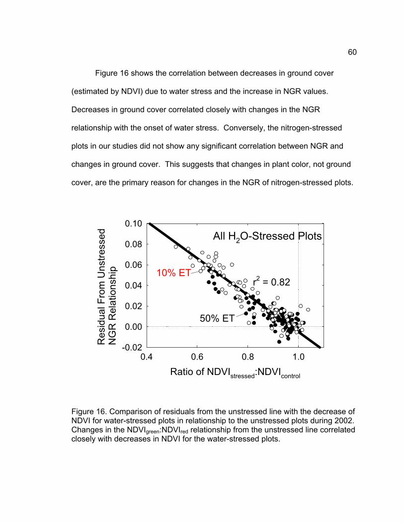
60
Figure 16 shows the correlation between decreases in ground cover
(estimated by NDVI) due to water stress and the increase in NGR values.
Decreases in ground cover correlated closely with changes in the NGR
relationship with the onset of water stress. Conversely, the nitrogen-stressed
plots in our studies did not show any significant correlation between NGR and
changes in ground cover. This suggests that changes in plant color, not ground
cover, are the primary reason for changes in the NGR of nitrogen-stressed plots.
Ratio of NDVIstressed:NDVIcontrol
0.4 0.6 0.8 1.0
Res
idua
l Fro
m U
nstre
ssed
N
GR
Rel
atio
nshi
p
-0.02
0.00
0.02
0.04
0.06
0.08
0.10
r2 = 0.82
50% ET
All H2O-Stressed Plots
10% ET
Figure 16. Comparison of residuals from the unstressed line with the decrease of NDVI for water-stressed plots in relationship to the unstressed plots during 2002. Changes in the NDVIgreen:NDVIred relationship from the unstressed line correlated closely with decreases in NDVI for the water-stressed plots.

61Identification of N Stress from Satellite Data
Figure 17 emphasizes the potential of the unstressed line as a plant stress
indicator. An IKONOS image collected on June 14, 2002 over a center pivot
wheat field in Idaho showed a marked separation between treatments of 0 and
65 kg ha-1 of applied nitrogen, and the unstressed nitrogen treatments. Although
many of the plots were approaching complete canopy cover, the deviations of the
stressed treatments from the unstressed NGR line at lower levels of ground
cover suggest that this method can be effective with partial ground cover as well
as complete ground cover.
ND
VIgr
een
0.50
0.55
0.60
0.65
0.70
NDVIred
0.70 0.72 0.74 0.76 0.78 0.80 0.82 0.84
ND
VI gr
een
0.50
0.55
0.60
0.65N
DVI
gree
n
0.50
0.55
0.60
0.65
NDVIred
0.70 0.72 0.74 0.76 0.78 0.80 0.82 0.84
ND
VI gr
een
0.50
0.55
0.60
0.65
0 kg N ha-1
65 kg N ha-1
150 kg N ha-1
195 kg N ha-1
Unstressed Line
Unstressed LineUnstressed Line
Unstressed Line
Figure 17. Comparison of the IKONOS NDVIgreen:NDVIred relationship for four nitrogen treatments with an unstressed line derived from control fertilizer treatment line on June 14, 2002. The 0 and 65 kg ha-1 nitrogen treatments deviated significantly from the unstressed line, while the 195 kg ha-1 treatment was almost identical to the 150 kg ha-1 control treatment.
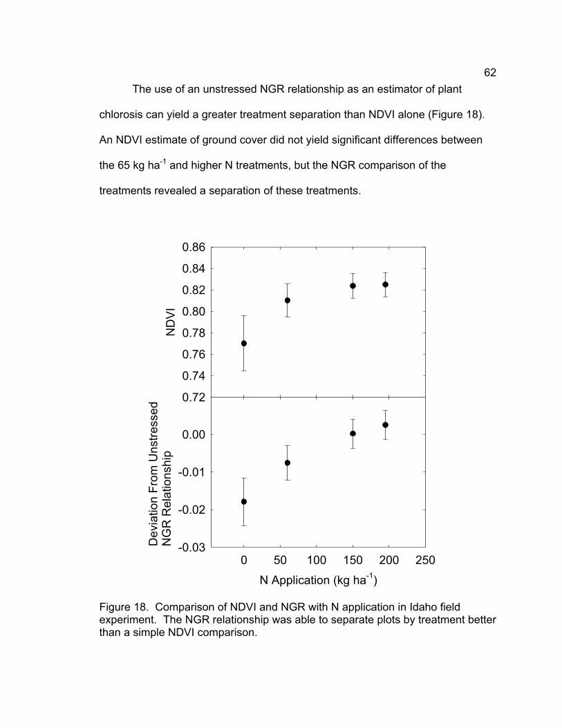
62The use of an unstressed NGR relationship as an estimator of plant
chlorosis can yield a greater treatment separation than NDVI alone (Figure 18).
An NDVI estimate of ground cover did not yield significant differences between
the 65 kg ha-1 and higher N treatments, but the NGR comparison of the
treatments revealed a separation of these treatments.
ND
VI
0.72
0.74
0.76
0.78
0.80
0.82
0.84
0.86
N Application (kg ha-1)
0 50 100 150 200 250
Dev
iatio
n Fr
om U
nstre
ssed
N
GR
Rel
atio
nshi
p
-0.03
-0.02
-0.01
0.00
Figure 18. Comparison of NDVI and NGR with N application in Idaho field experiment. The NGR relationship was able to separate plots by treatment better than a simple NDVI comparison.

63DISCUSSION
Advantages of the NGR Relationship
Separation of nitrogen-stressed wheat based on the relationship between
NDVIgreen and NDVIred allows identification of nitrogen stress separate from
ground cover. This method should allow identification of nitrogen stress without
having to resort to oblique measurements or derivative estimates. Because the
changes between the green and red regions of the spectrum are influenced by
the same factors that affect derivative indices, this method can offer a
comparable result without spectral smoothing and derivative calculations. This
technique was more useful than simple difference measurements, because both
the red and the green regions were normalized to the same point. Difference
indices are subject to the influence of slight changes in the relationship between
the reference reading and the crop reflectance reading, since even minor
changes in incident radiation can influence the magnitude of the reflectance.
Effects of Solar Angle
It is notable that all treatments during the 2001 growing season had a
more negative mean residual from the unstressed line on day 54 than on other
days (Figure 9), and a similar trend on day 47 during 2002 (Figure 10).
Measurements on these days were made early in the morning, when the solar
elevation was lower. Based on our studies, NDVIred is typically more sensitive to
solar angle than is NDVIgreen, resulting in a higher NDVIgreen:NDVIred relationship
for this day (Appendix 4). The effect of solar angle on plant canopy reflectance is
64an important issue in any type of plant health study. Middleton (1991) reported
that the response of vegetation indices to solar angle depends on canopy
structure, and that a general correction factor to remove sun angle effects is
inappropriate. Therefore, measurements should be made at similar solar angles.
Failure to do this can overshadow the small effects of changes in plant color.
Much of the variability due to solar angle can be eliminated on a day-to-day basis
if all of the plots are measured near the same time of day.
Comparison of Spectral Indices with Chlorophyll Content
The comparison of the NGR relationship values for each plot over the
growing season with SPAD measurements showed a higher correlation
throughout the growing season than the comparison of SPAD readings with
either NDVIred or NDVIgreen alone (Figure 13). This suggests that the NGR
relationship can increase the accuracy of chlorophyll concentration prediction.
Because NDVIred or NDVIgreen are closely related to ground cover, the
relationship of NDVIred or NDVIgreen alone with SPAD chlorophyll measurements
seems anomalous. However, much of this positive relationship is explained by
the fact that nitrogen stress decreases both leaf area and chlorophyll content,
resulting in a positive correlation between ground cover and chlorophyll content
for nitrogen-stressed plants. This relationship does not exist in water-stressed
wheat canopies, as shown in Figure 14.
65Satellite Data and the NGR Relationship
This technique was tested on only a limited basis with satellite data, but
the data suggests that satellites will be able to identify nitrogen-stressed plots
independent of ground cover, despite atmospheric effects and the broad band
nature of satellites (Figure 17). Both NDVIred and NDVIgreen are robust indices
that are based on the high-signal near-infrared regions of the spectrum. One
challenge is the identification of relatively slight changes in green reflectance of
stressed plots and the separation of this characteristic from other optical noise.
Another challenge for long-term estimates will be the correction of satellite data
to allow the comparison of NGR values between sampling dates.
Comparison of 2001 and 2002 unstressed lines
Unstressed plots from the 2001 and 2002 experiments had similar
normalized green:red relationships. Because the unstressed lines for the two
seasons were not statistically different, this method should allow a robust
estimate of plant health that can be used during multiple growing seasons.
However, the precise relationship between these parameters should be
determined based on individual field characteristics, such as soil color and plant
type. The measurement platform (satellite vs. ground-based) should also be
considered when identifying a specific NGR relationship for a field. As
mentioned earlier, solar angle should also be considered in making all ground
cover and plant color measurements. However, extensive calibration for a single

66set of measurements should not be necessary. Instead, an unstressed line can
be drawn through the data that with the highest NDVI values at a specific sample
time. Areas that have lower NDVI values than the unstressed plots can then be
identified as nitrogen or water-stressed based on their deviations from the
unstressed NGR relationship.
CONCLUSIONS
Simple ratio vegetation indices such as NDVI and RVI were found to have
similar predictive ability of ground cover as more complex indices over a
spectrally uniform soil background. However, NDVI was preferred over RVI for
this study because of its linear relationship with ground cover fraction before
canopy closure.
This research also identified a normalized method to compare green and
red reflectance of wheat canopies. The normalization minimizes the effects of
minor variations in incident radiation between reference and sample
measurements and allows the separation of nitrogen stress from the similar
spectral effects of ground cover fraction. This method may allow a broader
application of current leaf reflectance research to canopy-scale and field-scale
nutrient estimates.
References Adams, M.L., W.D. Philpot, and W.A. Norvell. 1999. Yellowness index: an
application of spectral second derivatives to estimate chlorosis of leaves in stressed vegetation. Int. J. Remote Sens. 20:3663-3675.

67Carter, G.A., and B.A. Spiering. 2002. Optical properties of intact leave for
estimating chlorophyll concentration. J. Environ. Qual. 31:1424-1432.
Curran, P.J. 1989. Remote sensing of foliar chemistry. Remote Sens. Environ. 30:271-278.
Demetriades-Shah, T.H., and M.N. Court. 1987. Oblique view reflectance for assessing nitrogen status of incomplete canopies. Int. J. Remote Sens. 8:1049-1055.
Demetriades-Shah, T.H., M.D. Steven, and J.A. Clark. 1990. High resolution derivative spectra in remote sensing. Remote Sens. Environ. 33:55-64.
Elvidge, C.D., and Z. Chen. 1995. Comparison of broad-band and narrow-band red and near-infrared vegetation indices. Remote Sens. Environ. 54:38-48.
Fernández, S., D. Vidal, E. Simón, and L. Solé-Sugrañes. 1994. Radiometric characteristics of Triticum aestivum cv. Astral under water and nitrogen stress. Int. J. Remote Sens. 15:1867-1884.
Gitelson, A.A., and M.N. Merzlyak. 1997. Remote estimation of chlorophyll content in higher plant leaves. Int. J. Remote Sens. 18:2691-2697.
Gitelson, A.A., and M.N. Merzlyak. 1998. Remote sensing of chlorophyll concentration in higher plant leaves. Adv. Space Res. 22:689-692.
Hinzman, L.D., M.E. Bauer, and C.S.T. Daughtry. 1986. Effects of nitrogen fertilization on growth and reflectance characteristics of winter wheat. Remote Sens. Environ. 19:47-61.
Horler, D.N.H., M. Dockray, and J. Barber. 1983. The red edge of plant leaf reflectance. Int. J. Remote Sens. 4:273-288.
Huete, A.R. 1988. A soil-adjusted vegetation index (SAVI). Remote Sens. Environ. 25:295-309.
Huete, A.R., R.D. Jackson, and D.F. Post. 1985. Spectral response of a plant canopy with different soil backgrounds. Remote Sens. Environ. 17:37-53.
Jackson, R.D., and P.J. Pinter. 1986. Spectral response of architecturally different wheat canopies. Remote Sens. Environ. 20:43-56.

68Jackson, R.D., P.N. Slater, and P.J. Pinter. 1983. Discrimination of growth and
water stress in wheat by various vegetation indices through clear and turbid atmospheres. Remote Sens. Environ. 13:187-208.
Jordan, C.F. 1969. Derivation of leaf area index from quality of light on the forest floor. Ecology 50:663-666.
Kauth, R.J., and G.S. Thomas. 1976. The tasseled cap -- A graphic description of the spectral-temporal development of agricultural crops as seen by Landsat. Proceedings of the Symposium on Machine Processing of Remotely Sensed Data, West Lafayette, IN:41-51.
Klassen, S.P., G. Ritchie, J. Frantz, D. Pinnock, and B. Bugbee. 2003. Real-time imaging of ground cover: relationships with radiation capture, canopy photosynthesis, and daily growth rate. In: Digital Imaging and Spectral Techniques: Applications to Precision Agriculture and Crop Physiology. (In press).
Major, D.J., F. Baret, and G. Guyot. 1990. A ratio vegetation index adjusted for soil brightness. Int. J. Remote Sens. 11:727-740.
Middleton, E.M. 1991. Solar zenith angle effects on vegetation indices in tallgrass prairie. Remote Sens. Environ. 38:45-62.
Monje, O., and B. Bugbee. 1992. Inherent limitations of nondestructive chlorophyll meters: a comparison of two types of meters. HortScience 27:69-71.
Neter, J., M.H. Kutner, C.J. Nachtsheim, and W. Wasserman. 1996. Applied linear statistical models. 4th ed. Irwin, Chicago.
Osborne, S.L., J.S. Schepers, D.D. Francis, and M.R. Schlemmer. 2002. Use of spectral radiance to estimate in-season biomass and grain yield in nitrogen- and water-stressed corn. Crop Sci. 42:165-171.
Otterman, J., T. Brakke, and J. Smith. 1995. Effects of leaf-transmittance versus leaf-reflectance on bi-directional scattering from canopy/soil surface: an analytical study. Remote Sens. Environ. 54:49-60.
Peñuelas, J., J.A. Gamon, A.L. Fredeen, J. Merino, and C.B. Field. 1994. Reflectance indices associated with physiological changes in nitrogen- and water-limited sunflower leaves. Remote Sens. Environ. 48:135-146.

69Peñuelas, J., J. Piñol, R. Ogaya, and I. Filella. 1997. Estimation of plant water
concentration by the reflectance water index WI (R900/R970). Int. J. Remote Sens. 18:2869-2875.
Pinter, P.J., G. Zipoli, G. Maracchi, and R.J. Reginato. 1987. Influence of topography and sensor view angles on NIR/red ratio and greenness vegetation indices of wheat. Int. J. Remote Sens. 8:953-957.
Richardson, A.J., and C.L. Weigand. 1977. Distinguishing vegetation from soil background information. Photogramm. Eng. Remote Sens. 43:1541-1552.
Rouse, J.W., R.H. Haas, J.A. Schell, and D.W. Deering. 1973. Monitoring vegetation systems in the great plains with ERTS, p. 309-317. Third ERTS Symposium, NASA SP-351, Vol. 1. NASA, Washington, DC.
Savitzky, A., and M.J.E. Golay. 1964. Smoothing and differentiation of data by simplified least squares procedures. Anal. Chem. 36:1627-1639.
Taiz, L., and E. Zeiger. 2002. Plant physiology. 2nd ed. Sinauer Associates, Sunderland, MA.
Tucker, C.J. 1979. Red and photographic infrared linear combinations for monitoring vegetation. Remote Sens. Environ. 8:127-150.
Yoder, B.J., and R.E. Pettigrew-Crosby. 1995. Predicting nitrogen and chlorophyll content and concentrations from reflectance spectra (400-2500 nm) at leaf and canopy scales. Remote Sens. Environ. 53:199-211.

70CHAPTER 4
SUMMARY
Reflectance of red and green radiation by plants is heavily influenced by
chlorophyll absorption. Spectral reflectance of plant canopies provides an
accurate indication of ground cover fraction, which is highly correlated with
radiation capture. If nutrients and water do not limit growth, radiation capture is
highly correlated with daily growth rate and ultimate yield. However, none of the
common vegetation indices are able to separate a more developed, stressed
canopy from a less-developed, rapidly growing canopy.
Nitrogen stress is highly correlated with reduced chlorophyll concentration
and increased reflectance of green radiation, while water stress inhibits leaf
expansion can increases chlorophyll concentration and decrease green
reflectance. All but one of the 10 common spectral indices that we tested
accurately determined ground cover, but we found that none of them could
distinguish the intensity of leaf color from ground cover fraction. Here we report
a reflective index that can differentiate nitrogen and water stress over a wide
range of ground cover. The index is based on the ratio of the green and red
variants of the normalized difference vegetation index (NDVIgreen/NDVIred). The
normalization minimizes the effects of minor variations in incident radiation
between reference and sample measurements and allows the separation of
nitrogen stress from the similar spectral effects of ground cover fraction. This
method may allow a broader application of current leaf reflectance research to
canopy-scale and field-scale nutrient estimates.

71The new index was able to distinguish N and water stress from satellite
data using wavelengths less than 1000 nm. This index should be broadly
applicable over a wide range of plant types and environments. The issues of
solar angle and soil background color were also examined to determine their
effects on plant reflectance measurements.

72
APPENDICES

73APPENDIX 1: PREDICTING GROUND COVER AND YIELD
ABSTRACT
Crop yield estimates are useful for many aspects of crop production,
including marketing, storage planning, and identification of stress. An accurate
yield estimate can be a valuable production tool. Two promising methods of yield
estimation are radiometric remote sensing and digital imaging. The dominant
factors in crop yield are the quantity of incident radiation and the absorptive
ability of the crop canopy. Vegetation indices based on the reflective properties
of plants have been used for several years to estimate ground cover. These
ground cover estimates can be used to calculate yield based on the close
relationship between ground cover and a crop canopy’s absorptive capacity
during the growing season. Photographic images can also be used to determine
plant ground cover and measure plant stress for GIS applications. Like spectral
indices, photographs determine ground cover to estimate crop radiation
absorption. Photographic images are less sensitive to soil color, provided that
plants are visually separable from the background. Common vegetation indices
(red NDVI, green NDVI, and RVI) and digital image estimates of plant ground
cover were tested for their ability to predict crop yield for spring wheat test plots.
Digital image estimates of ground cover were also compared with vegetation
indices to ascertain which indices correlate most closely with imaged ground
cover. All indices showed high correlation with final yield prior to anthesis, with
RVI providing a slightly more linear prediction of final yield based on vegetation

74cover than the other indices. Digital images and indices showed similar
correlation with final yield until awn emergence (day 60), after which vegetation
indices became a more accurate predictor of final yield. The vegetation indices
that correlated most closely with digital images of ground cover included green
and red NDVI, SAVI, RVI, and DVI.
INTRODUCTION
Plant radiation capture limits all other components of yield potential for an
unstressed plant (Volk et al., 1995). Radiation absorption by plants is a function
of canopy cover, plant architecture, and leaf absorption efficiency. Plant
phenology and leaf absorption efficiency remain relatively constant within a
species at a given growth stage (Baret et al., 1987), so canopy cover should be
an accurate estimator of radiation absorption. Canopy cover can also be used as
a predictor of final yield, because the majority of plant growth components are
controlled by plant cover. The primary plant stresses decrease yield by inhibiting
canopy growth. Water limitations limit plant growth at several levels. Mild water
stress has a dramatic effect on leaf expansion rate prior to any effects on leaf
photosynthetic rate or translocation rate through the phloem (Taiz and Zeiger,
1998). Nitrogen deficiency decreases crop yield and quality by limiting amino
acid and chlorophyll synthesis, resulting in growth inhibition and leaf senescence
(Marschner, 1995).
Plant canopy imaging provides a quick, nondestructive method for
determining plant growth. Because photographic imaging is relatively simple, it

75has been used in many remote sensing applications as a method for determining
ground cover, and as a standard upon which to base the success of other
imaging types, such as satellite imagery and radiometric applications. Overhead
photography is useful as a total ground cover estimator, but also as an indicator
of spatial variability in ground cover (Blazquez et al., 1981; Stone et al., 1988).
Beverly (1996) suggested that plant vigor estimates provide a more direct and
integrative indication of plant response to soil properties and management than
does soil testing.
Past experimental methods for determining ground cover include line-
transect analysis, meterstick measurements, and photographic grid testing
(Hayes and Han, 1993). Ground cover has also been estimated in the laboratory
by comparison of photos with photos of known ground cover or by superimposing
a grid with a photograph or a projected slide of an area. Each of these methods
requires an observer to visually determine whether each specified point in the
picture is soil or plant, a process that is time consuming and impractical for most
applications. These methods are also subject to human perspective and error.
Machine vision methods have been used to differentiate between plants and soil
via thresholding (Hayes and Han, 1993; Olthof and King, 2000; Stone et al.,
1988), but they can be prone to error as soil and plant colors change (Hayes and
Han, 1993).
Recent advances in image manipulation software allow the union of visual
discrimination and computer thresholding. This speeds up the separation

76process between leaf and background and allows a visual cross-check of
accuracy.
Potential Errors in Ground Cover Estimation
One potential ground cover measurement error in near-remote imaging
(<5 m) involves vertical plant growth. The apparent size of an object increases
as it approaches the camera proportional to the distance formula, d12/d2
2, where
d1 is the original distance from the camera to the object, and d2 is the new
distance to the object. Plants growing toward a set camera increase in apparent
size and cause the overestimation of ground cover. This problem is negligible if
plant growth is small in comparison to the distance from the camera to the plant,
but can result in large errors if the camera is close to the plants.
Another difficulty that may arise in image analysis is shadowing (Hayes
and Han, 1993). Shadowing makes discrimination between leaf and ground
difficult. Several methods can be used in small plots to minimize problems from
shadowing. Pictures can be taken under low light with a camera flash on to align
the camera line of sight with the primary light incident to the plant leaves.
Alternatively, pictures can be taken on cloudy days, a barrier may be used to
block direct lighting, or the camera can be placed in line with the light source.
These methods are most effective if the camera lens remains perpendicular to
the ground.
Spectral estimates of ground cover are also influenced by outside factors.
One common confounding factor in ground cover estimation using spectral

77indices is the influence of soil color (Huete, 1988; Huete et al., 1985). During
early stages of growth, the soil constitutes a large portion of canopy reflectance.
The primary variable in soil reflectance is brightness, because nearly all spectral
data for a soil falls along a line extending from the origin (Kauth and Thomas,
1976). High reflecting, light-colored soils influence indices more than do dark,
low-reflecting soils (Jackson et al., 1983). Spectral differences between soils
may be attributed to variations in surface moisture, particle size distribution, soil
mineralogy, soil structure, surface roughness, crusting and presence of shadow
(Huete et al., 1984; Huete et al., 1985).
MATERIALS AND METHODS
Spring wheat (Triticum aestivum cv. Westbred 936) was planted April 8,
2002 at the Greenville Farm research plots in Logan, Utah, at a density of 112 kg
per ha-1. Treatment transects consisted of four randomized replicates of each
fertilizer treatment listed in Table 6.
Table 6 Summer 2002 treatments
Treatment Fertilizer Control No nitrogen or phosphorus added
Phosphorus 67 kg phosphorus ha-1
Nitrogen 67 kg nitrogen ha-1
Nitrogen/Phosphorus 67 kg nitrogen 28 kg phosphorus ha-1

78
15O
1.25 m0.27 m
0.75 m
15O
1.25 m0.27 m
0.75 m
Computer
Spectrometer
Black PVC swing arm
Fiber optic cable
Figure 19. Sensor mounting design for summer 2002 tests. A rigid swing arm positioned the sensor over the canopy away from the wheelbarrow.
The line-source irrigation method was used to introduce varying levels of water
stress in the plots. Measurements were performed on 64 sample points – four in
each replicate treatment. The sample points included both water-sufficient and
water-deficient plots.
On seventeen dates during the growing season, each plot was
photographed from above (height = 1.5 m), and the pictures were analyzed for
ground cover. Ground cover analysis was performed in Adobe Photoshop 6.0®
(Adobe Systems, Inc., San Jose, CA). Soil was selectively erased using the
magic eraser tool, the magic wand tool, or the box selection tool. Selection
tolerances generally ranged from 10 to 35, depending on the soil homogeneity
and the soil/plant contrast. After soil elimination, ground cover was estimated
using the histogram function. In addition, growth stage was recorded and based
on the Zadoks growth staging parameters (Zadoks et al., 1974).

79Reflectance measurements were made using a StellarNet EPP2000
visible/NIR spectrometer with fiber optic cable (StellarNet, Inc., Tampa, FL). The
spectrometer was mounted in a wheelbarrow, and the cable was attached to the
end of a rigid metal support arm that was 1.25 m high and extended 0.75 m over
the plots (Figure 19). A reference standard made of pressed
polytetrafluoroethylene (PTFE) was used to measure incident radiation, and
reflectance ratio was calculated as the ratio of reflected to incident radiation.
Reflectance data was smoothed using a five nanometer Savitzky-Golay filter at
the time of collection (Savitzky and Golay, 1964). Spectral indices were
calculated in Microsoft Excel® (Microsoft Corp., Redmond, WA), and broadband
variants of narrowband indices were calculated from integrated reflectance over
the broadband intervals. The broadband intervals were based on Landsat band
intervals (Kauth and Thomas, 1976).
At harvest, 1 meter square plots were harvested at each sample point.
The wheat was dried and threshed, and the seed mass for each plot was
recorded. Protein analysis was performed on a sub sample of each plot sample.
Final plot yield was compared to the in-season NDVI and ground cover
measurements.
Yield and Ground Cover
Final yield was compared with spectral indices and ground cover
estimates of each measurement date by determining the linear correlation (r2) of

80final yield with NDVI. The slope and intercept of the correlation line were also
compared by date and growth stage.
In addition, yield was estimated from the integrated NDVI of each plot over
the growing season. A light bar was used to measure canopy reflectance and
transmittance of photosynthetically active radiation (PAR) for wheat plots on four
days, and a spectrometer was used to calculate NDVI. The absorbance of PAR
was calculated by the following formula:
groundreftransrefincabs PARPARPARPARPAR −+−−= [4]
PAR absorbance was correlated with NDVI, and the slope of the
correlation line was used to estimate PAR absorbance at all NDVI values
throughout the growing season. Integrated PAR absorbance was calculated by
integrating the values at the midpoint between each measurement over the
course of the growing season.
RESULTS AND DISCUSSION
2001
The linear correlation of NDVI with final yield increased with time until it
reached a maximum of 0.70 on June 20 (Zadoks 71), after which the correlation
decreased (Table 7). The slope of correlation between yield and NDVI increased
until June 14 (Zadoks 62), then decreased until the end of the study. Intercepts
for this study were negative until late in the study.
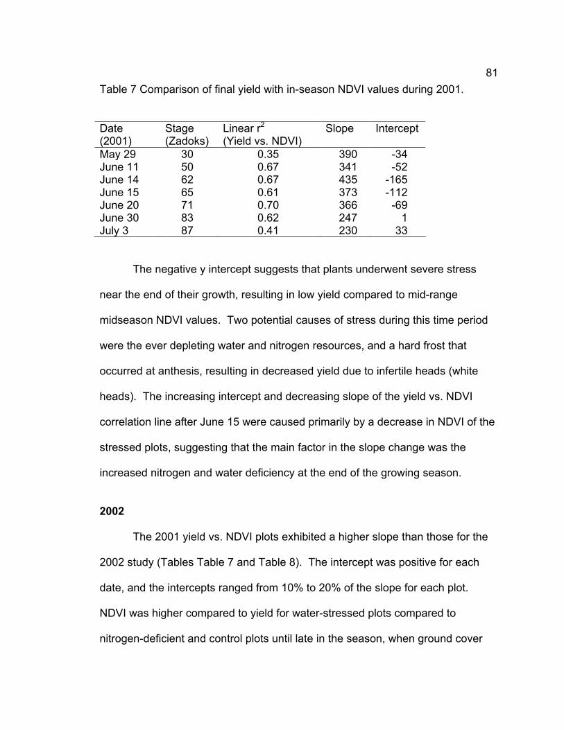
81Table 7 Comparison of final yield with in-season NDVI values during 2001.
Date (2001)
Stage (Zadoks)
Linear r2 (Yield vs. NDVI)
Slope Intercept
May 29 30 0.35 390 -34 June 11 50 0.67 341 -52 June 14 62 0.67 435 -165 June 15 65 0.61 373 -112 June 20 71 0.70 366 -69 June 30 83 0.62 247 1 July 3 87 0.41 230 33
The negative y intercept suggests that plants underwent severe stress
near the end of their growth, resulting in low yield compared to mid-range
midseason NDVI values. Two potential causes of stress during this time period
were the ever depleting water and nitrogen resources, and a hard frost that
occurred at anthesis, resulting in decreased yield due to infertile heads (white
heads). The increasing intercept and decreasing slope of the yield vs. NDVI
correlation line after June 15 were caused primarily by a decrease in NDVI of the
stressed plots, suggesting that the main factor in the slope change was the
increased nitrogen and water deficiency at the end of the growing season.
2002
The 2001 yield vs. NDVI plots exhibited a higher slope than those for the
2002 study (Tables Table 7 and Table 8). The intercept was positive for each
date, and the intercepts ranged from 10% to 20% of the slope for each plot.
NDVI was higher compared to yield for water-stressed plots compared to
nitrogen-deficient and control plots until late in the season, when ground cover

82decreased due to water stress. This feature decreased the slope of the
correlation graphs, because water-stressed plots appeared had high NDVI and
low final yield. The correlation values of unstressed plots were highest on and
after June 13 (Zadoks 60). Vegetation indices and digital image ground cover
estimates showed similar correlation with final yield until approximately anthesis.
After anthesis, the spectrometer vegetation indices correlated more closely with
final yield than did digital images (Figure 23).
ND
VI
0 .0
0.2
0.4
0.6
0.8
Days After P lanting20 30 40 50 60 70
ND
VI
0 .0
0.2
0.4
0.6
0.8
Unstressed
W ater-stressed
Unstressed
Nitrogen-stressed
Figure 20. Comparison of NDVI during 2002 growing season for unstressed, nitrogen-stressed, and water-stressed plots.
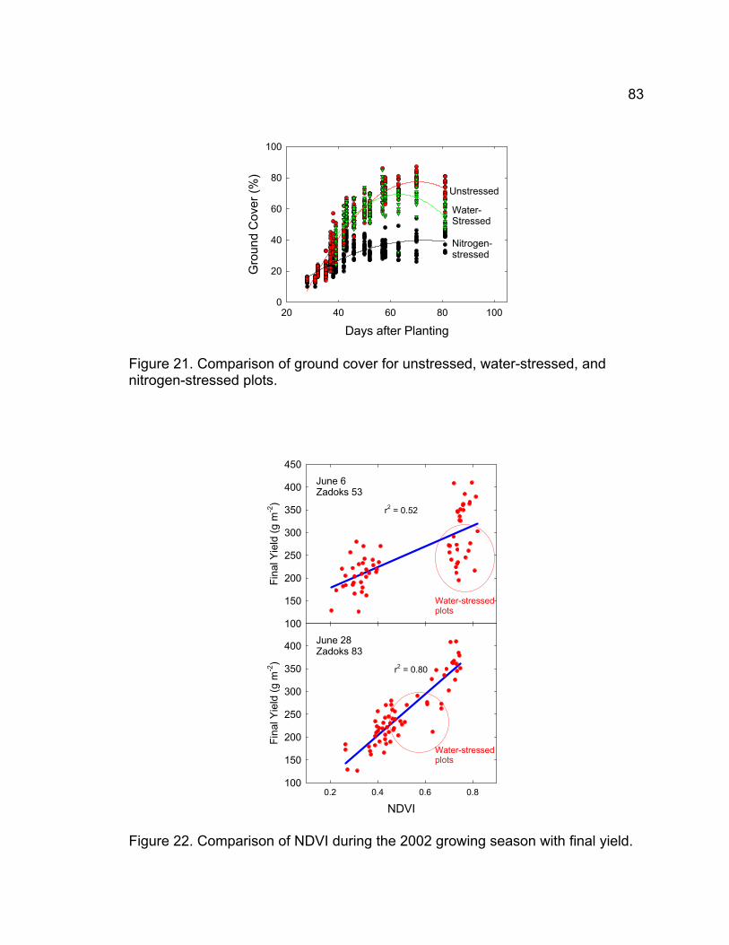
83
Days after Planting20 40 60 80 100
Gro
und
Cov
er (%
)
0
20
40
60
80
100
Nitrogen-stressed
Unstressed
Water-Stressed
Figure 21. Comparison of ground cover for unstressed, water-stressed, and nitrogen-stressed plots.
Fina
l Yie
ld (g
m-2
)
100
150
200
250
300
350
400
450June 6Zadoks 53
NDVI0.2 0.4 0.6 0.8
Fina
l Yie
ld (g
m-2
)
100
150
200
250
300
350
400 June 28Zadoks 83
r2 = 0.52
r2 = 0.80
Water-stressedplots
Water-stressedplots
Figure 22. Comparison of NDVI during the 2002 growing season with final yield.

84
Table 8 Relationship between NDVI and final yield during 2002 by date.
Date (2002)
Days after planting
Stage (Zadoks)
Linear r2 (Yield vs. NDVI)
Slope Intercept
6 May 28 13 0.03 9 May 31 21 0.05
13 May 35 23 0.10 15 May 37 30 0.21 16 May 38 30 0.26 17 May 39 31 0.15 18 May 40 31 0.25 20 May 42 32 0.13 21 May 43 32 0.31 23 May 45 32 0.22 24 May 46 33 0.36 25 May 47 33 0.30 28 May 50 41 0.39 267 116 29 May 51 41 0.42 284 91 30 May 52 45 0.42 261 115 3 June 54 49 0.56 274 86 4 June 56 50 0.53 246 107 5 June 57 52 0.53 241 119 6 June 58 53 0.52 227 133
13 June 66 60 0.62 289 86 14 June 67 61 0.62 284 98 17 June 70 69 0.72 336 65 19 June 72 71 0.77 379 26 20 June 73 73 0.74 362 40 23 June 76 75 0.80 390 41 25 June 78 80 0.80 406 39 28 June 81 83 0.80 448 25

85
Days After Planting20 30 40 50 60 70 80 90
Cor
rela
tion
(r2 )
0.0
0.2
0.4
0.6
0.8
1.0
NDVIOnset ofN stress
Onset ofH20 stress
MaximumGround Cover
GroundCover
Figure 23. Correlation of NDVI and ground cover with final seed yield (summer 2002).
INTEGRATED ABSORPTION AND CROP YIELD
The integrated absorption of radiation by each plot was estimated by NDVI
values. Previous studies of wheat with satellite imagery have compared NDVI
with final yield, but no relationship between NDVI and absorption has been
discussed. Discussion: note that estimated yield was higher than predicted yield
for most water stressed plots. Compare this with Boissard’s paper on ear hydric
status after anthesis. Because ear hydric status after anthesis can affect yield

86dramatically, this probably explains why the estimated yield was higher than the
actual yield for these plots. The following references relate to NDVI and yield
estimates… (Benedetti and Rossini, 1993; Boissard et al., 1993; Labus et al.,
2002; Manjunath et al., 2002)
NDVI0.0 0.2 0.4 0.6 0.8 1.0
Rad
iatio
n A
bsor
ptio
n (%
)
0
20
40
60
80
100
y = 111x -13.5
y = 280x -150
Water-Stressed
Figure 24. Correlation of NDVI with radiation absorption estimates based on light bar measurements. At high NDVI values (above 0.8), radiation absorption slope increased.
Actual Yield100 150 200 250 300 350 400 450
Pre
dict
ed Y
ield
100
150
200
250
300
350
400
450
y=1.02xr2=0.70
Nitrogen-Stressed
Control
Figure 25. Comparison of actual and predicted yield based on radiation absorption model.

87The high correlation values for unstressed plots at anthesis suggest that
predictions of plant yield can be highly accurate at anthesis if plant stress does
not occur afterwards. Although NDVI became a less accurate predictor of yield
after anthesis in 2001 (Table 7), much of this may have been due to early leaf
senescence due to the long period of plant stress observed in this experiment.
Correlation did not show a decrease during the 2002 test with time, suggesting
that the onset of stress can be identified well into dough development.
The peak correlation of ground cover with final yield at anthesis agrees
with Dusek et al. (1985), who state that ground cover has a peak correlation with
plant biomass near anthesis. The superior correlation of NDVI with final yield
after anthesis may be due to the ability of this vegetation index to estimate only
green, actively photosynthetic tissue. The digital images do not discriminate
yellow leaves from green leaves, resulting in higher variability due to early
senescence of leaves on stressed plants.
REFERENCES
Baret, F., I. Champion, G. Guyot, and A. Podaire. 1987. Monitoring wheat canopies with a high spectral resolution radiometer. Remote Sens. Environ. 22:367-378.
Benedetti, R., and P. Rossini. 1993. On the use of NDVI profiles as a tool for agricultural statistics: the case study of wheat yield estimate and forecast in Emilia Romagna. Remote Sens. Environ. 45:311-326.
Beverly, R.B. 1996. Video image analysis as a nondestructive measure of plant vigor for precision agriculture. Commun. Soil. Sci. Plant Anal. 27:607-614.

88Blazquez, C.H., R.A. Elliot, and G.J. Edwards. 1981. Vegetable crop
management with remote sensing. Photogramm. Eng. Remote Sens. 47:543-547.
Boissard, P., J.-G. Pointel, and P. Huet. 1993. Reflectance, green leaf area index and ear hydric status of wheat from anthesis until maturity. Int. J. Remote Sens. 14:2713-2739.
Dusek, D.A., R.D. Jackson, and J.T. Musick. 1985. Winter wheat vegetation indices calculated from combinations of seven spectral bands. Remote Sens. Environ. 18:255-267.
Hayes, J.C., and Y.J. Han. 1993. Comparison of crop-cover measuring systems. Trans. ASAE 36:1727-1732.
Huete, A.R. 1988. A soil-adjusted vegetation index (SAVI). Remote Sens. Environ. 25:295-309.
Huete, A.R., D.F. Post, and R.D. Jackson. 1984. Soil spectral effects on 4-space vegetation discrimination. Remote Sens. Environ. 15:155-165.
Huete, A.R., R.D. Jackson, and D.F. Post. 1985. Spectral response of a plant canopy with different soil backgrounds. Remote Sens. Environ. 17:37-53.
Jackson, R.D., P.N. Slater, and P.J. Pinter. 1983. Discrimination of growth and water stress in wheat by various vegetation indices through clear and turbid atmospheres. Remote Sens. Environ. 13:187-208.
Kauth, R.J., and G.S. Thomas. 1976. The tasseled cap -- A graphic description of the spectral-temporal development of agricultural crops as seen by Landsat. Proceedings of the Symposium on Machine Processing of Remotely Sensed Data:41-51.
Labus, M.P., G.A. Nielsen, R.L. Lawrence, R. Engel, and D.S. Long. 2002. Wheat yield estimates using multi-temporal NDVI satellite imagery. Int. J. Remote Sens. 23:4169-4180.
Manjunath, K.R., M.B. Potdar, and N.L. Purohit. 2002. Large area operational wheat yield model development and validation based on spectral and meteorological data. Int. J. Remote Sens. 23:3023-3038.
Marschner, H. 1995. Mineral nutrition of higher plants. 2nd ed. Academic Press, San Diego.

89Olthof, I., and D.J. King. 2000. Development of a forest health index using
multispectral airborne digital camera imagery. Can. J. of Remote Sens. 26:166-176.
Savitzky, A., and M.J.E. Golay. 1964. Smoothing and differentiation of data by simplified least squares procedures. Anal. Chem. 36:1627-1639.
Stone, D.A., B. Lancashire, R.A. Sutherland, K.B. Niendorf, and R.B. Sampson. 1988. A low cost microcomputer-based image analysis system for the measurement of percentage ground cover. Research and Development of Agriculture 5:65-70.
Taiz, L., and E. Zeiger. 1998. Plant Physiology. 2nd ed. Sinauer Associates, Sunderland, MA.
Volk, T., R. Wheeler, and B. Bugbee. 1995. An approach to crop modeling with the energy cascade. Life Support and Biosphere Science 1:119-127.
Zadoks, J.C., T.T. Chang, and C.F. Konzak. 1974. A decimal code for the growth stages of cereals. Weed Res. 14:415-421.
90APPENDIX 2: LEAF REFLECTANCE, TRANSMITTANCE
AND CHLOROPHYLL CONCENTRATION
ABSTRACT
Chlorophyll concentration is a useful indicator of plant health and nitrogen
concentration. Transmittance and reflectance of visible and NIR radiation are
commonly used to estimate chlorophyll concentration of plant leaves.
Chlorophyll concentration is commonly estimated using differential transmittance
of multiple visible and NIR wavelengths. However, more research during the
past few years has focused on reflectance as an indicator of chlorophyll
concentration. This study compared the accuracy of transmittance and
reflectance measurements in determining leaf chlorophyll concentration of spring
wheat (Triticum aestivum cv. Westbred 936). Normalized reflectance and
transmittance data showed a similar linear correlation with leaf chlorophyll
concentration (highest r2=0.90 and 0.91, respectively). However, reflectance
data required normalization to a wavelength to attain this high correlation, while
transmittance data did not.
INTRODUCTION
Chlorophyll properties dominate leaf reflectance and transmittance of
visible radiation. Nitrogen is a principle component of chlorophyll (Taiz and
Zeiger, 1998), and chlorophyll concentration often correlates closely with nitrogen
concentration in plant leaves (Costa et al., 2001; Fernández et al., 1994; Filella et

91al., 1995; Serrano et al., 2000). Chlorophyll absorbs the majority of incident red
and blue radiation, resulting in little red or blue reflectance by green vegetation.
The blue absorbance peak of chlorophyll overlaps with the absorbance of
carotenoids, so blue reflectance is not generally used to estimate chlorophyll
concentration (Sims and Gamon, 2002). Maximum red absorbance occurs
between 660 and 680 nm (Curran, 1989), but relatively low chlorophyll
concentrations can saturate this absorption region (Sims and Gamon, 2002).
Therefore, chlorophyll concentration is usually predicted from reflectance in the
550 nm or 700 nm ranges, because these regions require higher chlorophyll
concentrations to saturate. Leaf chlorophyll concentration has also been well-
correlated with reflectance in the green and red spectral regions. Leaf
reflectance factors in the 550 nm and 660 nm range show high correlation with
leaf nitrogen concentration (Fernández et al., 1994) and chlorophyll
concentration (Adams et al., 1999). The shape of the visible reflectance spectra
of leaves changes between the maximum reflectance near 550 nm and the
minimum near 660 nm as they become chlorophyll-deficient, and changes in this
shape can also be used to identify chlorosis in some instances (Adams et al.,
1999; Carter and Spiering, 2002).
Leaf mesophyll reflects a large proportion of NIR radiation (Huete et al.,
1984; Taiz and Zeiger, 1998). The region of rapid increase in reflectance
between the red and infrared regions of the spectrum, called the red edge, is
frequently used to indicate plant health (e.g. Dawson and Curran, 1998; Horler et
al., 1983a; Horler et al., 1983b; Jago et al., 1999). Horler et al. (1983b) observed

92that chlorophyll concentration in leaves correlated with the maximum slope of
reflectance at the boundary between the red and NIR spectral domains. Spectral
indices have been derived for both single-leaf and plant canopy reflectance
measurements. Single-leaf measurements offer the advantage of higher signal-
to-noise ratio and more control over the operating environment, while canopy
measurements allow measurements over a broader scale.
MATERIALS AND METHODS
Wheat plants were grown at seven nitrogen treatments to allow a wide
range of leaf chlorophyll concentration. At heading, the reflectance of the top two
or three leaves for the main stem of each plant was measured using an ASD
FieldSpec Pro spectrometer with high-intensity contact probe (ASD, Boulder,
CO). Transmittance of the leaves was also measured using a StellarNet
EPP2000 VIS/NIR spectrometer (StellarNet, Inc. Tampa, FL) with a custom-built
transmittance probe, and a SPAD-502 chlorophyll meter (Minolta, Ramsey, NJ).
After measurements, 15-mm wide circles were cut from each measured leaf.
Chlorophyll was extracted from each leaf disk in 7 mL DMSO and an incubation
period of 30 minutes (Hiscox and Israelstam, 1979). The extractions were stored
at 4o C for 2 days, then analyzed for chlorophyll concentration using the method
described by Porra et al. (1989).

93RESULTS
Leaf transmittance and reflectance of green and far-red radiation showed
a high linear correlation (highest r2=0.91) with tissue chlorophyll concentrations.
Normalized and raw transmittance data showed similar correlation to chlorophyll
concentration by wavelength, with the maximum correlation in the green and red-
edge regions of the transmittance spectrum (Figure 26).
Raw reflectance data showed significantly lower correlation and different
peak correlation wavelengths than normalized data. One likely reason for this
deviation is that leaves did not fill the entire viewing area of the ASD reflectance
probe. Normalization should be performed prior to wavelength analysis to
increase the accuracy of reflectance in estimating leaf chlorophyll concentration
when using this setup. Chlorophyll concentration correlated well with normalized
leaf transmittance and reflectance (highest r2 = 0.91). Both reflectance and
transmittance showed a decreased correlation value in the red, with correlation
minima occurring near 675 nm. The correlation (r2) minimum for leaf reflectance
was 0.08, and the correlation minimum for leaf transmittance was 0.67 (Figure
26).

94
Col 14 vs RSQNunnorm Col 14 vs RSQP Col 1 vs Unnorm
Col 1 vs Norm820
Col 1 vs Unnorm
Col 1 vs Norm820
Wavelength (nm)400 500 600 700 800 900 1000
Cor
rela
tion
(r2 )
0.0
0.2
0.4
0.6
0.8
1.0
Cor
rela
tion
(r2 )
0.0
0.2
0.4
0.6
0.8
1.0
Raw Data
Raw Data
(557,0.91) (707,0.91)
(557,0.82)(722,0.90)
Typical LeafReflectance
Typical LeafTransmittance
Leaf Transmittance vs. Chlorophyll
Leaf Reflectance vs. Chlorophyll
Standardized to 820 nm
Standardized to 940 nm
Figure 26. Comparison of leaf reflectance and transmittance with chlorophyll concentration.

95
R72
2/R82
0
0.55
0.60
0.65
0.70
0.75
0.80
0.85
Chlorophyll Content (mg m-2)250 300 350 400 450 500 550 600 650
T 707/T
940
0.2
0.3
0.4
0.5
Leaf Reflectancenormalized to 820 nm
Leaf Transmittancenormalized to 940 nm
y = -6.39E-4 x + 0.979r2=0.90
y = -8.98E-4 x + 0.803r2=0.91
Figure 27. Correlation of normalized leaf reflectance and transmittance with leaf chlorophyll concentration.
96DISCUSSION
Chlorophyll concentration correlated well with normalized leaf
transmittance and reflectance (highest r2 = 0.91). Both reflectance and
transmittance showed a decreased correlation value in the red, with correlation
minima occurring near 675 nm. This agrees with the work of Carter and Spiering
(2002), who noted the trend but did not account for their findings. Sims and
Gamon (2002) offer an explanation for this phenomenon, stating that relatively
low chlorophyll concentrations are sufficient to saturate absorption in the 660-680
nm range, which reduces the sensitivity of these wavelengths for determining
high chlorophyll concentrations. The data from this experiment supported this
idea, because deviations occurred at the higher chlorophyll concentrations.
REFERENCES
Adams, M.L., W.D. Philpot, and W.A. Norvell. 1999. Yellowness index: an application of spectral second derivatives to estimate chlorosis of leaves in stressed vegetation. Int. J. Remote Sens. 20:3663-3675.
Carter, G.A., and B.A. Spiering. 2002. Optical properties of intact leave for estimating chlorophyll concentration. J. Environ. Qual. 31:1424-1432.
Costa, C., L.M. Dwyer, P. Dutilleul, D.W. Stewart, B.L. Ma, and J.D. Smith. 2001. Inter-relationships of applied nitrogen, spad, and yield of leafy and non-leafy maize genotypes. J. Plant Nutr. 24:1173-1194.
Curran, P.J. 1989. Remote sensing of foliar chemistry. Remote Sens. Environ. 30:271-278.
Dawson, T.P., and P.J. Curran. 1998. A new technique for interpolating the reflectance red edge position. Int. J. Remote Sens. 19:2133-2139.

97Fernández, S., D. Vidal, E. Simón, and L. Solé-Sugrañes. 1994. Radiometric
characteristics of Triticum aestivum cv. Astral under water and nitrogen stress. Int. J. Remote Sens. 15:1867-1884.
Filella, I., L. Serrano, J. Serra, and J. Penuelas. 1995. Evaluating wheat nitrogen status with canopy reflectance indices and discriminant analysis. Crop Sci. 35:1400-1405.
Hiscox, J.D., and G.F. Israelstam. 1979. A method for the extraction of chlorophyll from leaf tissue without maceration. Can. J. Bot. 57:1332-1334.
Horler, D.N.H., M. Dockray, and J. Barber. 1983a. The red edge of plant leaf reflectance. Int. J. Remote Sens. 4:273-288.
Horler, D.N.H., M. Dockray, J. Barber, and A.R. Barringer. 1983b. Red edge measurements for remotely sensing plant chlorophyll content. Adv. Space Res. 3:273-277.
Huete, A.R., D.F. Post, and R.D. Jackson. 1984. Soil spectral effects on 4-space vegetation discrimination. Remote Sens. Environ. 15:155-165.
Jago, R.A., M.E.J. Cutler, and P.J. Curran. 1999. Estimating canopy chlorophyll concentration from field and airborne spectra. Remote Sens. Environ. 68:217-224.
Porra, R.J., W.A. Thompson, and P.E. Kriedemann. 1989. Determination of accurate extinction coefficients and simultaneous equations for assaying chlorophylls a and b extracted with four different solvents: verification of the concentration of chlorophyll standards by atomic absorption spectroscopy. Biochim. Biophys. Acta. 975:384-394.
Serrano, L., I. Filella, and J. Penuelas. 2000. Remote sensing of biomass and yield of winter wheat under different nitrogen supplies. Crop Sci. 40:723-731.
Sims, D.A., and J.A. Gamon. 2002. Relationships between leaf pigment content and spectral reflectance across a wide range of species, leaf structures and developmental stages. Remote Sens. Environ. 81:337-354.
Taiz, L., and E. Zeiger. 1998. Plant Physiology. 2nd ed. Sinauer Associates, Sunderland, MA.

98APPENDIX 3: BACKGROUND EFFECTS
ON SPECTRAL INDICES
ABSTRACT
Vegetation indices that measure plant growth are based on deviations
from the reflectance of a bare soil to a plant-covered soil. Spectral indices such
as the normalized difference vegetation index (NDVI) correlate well with ground
cover and leaf area index (LAI) for a particular soil, but can be widely different for
the same crop with a different soil color. Previous research has attempted to
minimize this effect. Indices used to correct for the soil background include
perpendicular vegetation indices (PVI), the soil-adjusted vegetation index (SAVI),
and derivative vegetation indices. These indices treat the soil as a reflective
medium that has a nearly linear slope in the visible and NIR spectral regions.
However, many plants are grown on backgrounds that do not match the typical
soil line. Examples include greenhouse plants and row crops that have plastic
placed under them. The objective of this study was to evaluate vegetation
indices with standard and nonstandard reflective backgrounds to determine
which index best determines leaf area index over nonstandard backgrounds.
Backgrounds included white, red, gray, soil-covered, and black. It was
determined that the best indicators of LAI over a wide variety of backgrounds
were the difference vegetation index and SAVI with custom coefficients. An
alternative method of mathematically subtracting the background from the

99plant/background spectrum was examined, and this method increased the
correlation between LAI and spectral indices.
INTRODUCTION
A significant issue in whole-canopy reflectance experiments is the
variation between green plant cover and the soil background. High reflecting,
light-colored soils influence indices more than do dark, low-reflecting soils
(Jackson et al., 1983). Spectral differences between soils may be attributed to
variations in surface moisture, particle size distribution, soil mineralogy, soil
structure, surface roughness, crusting and presence of shadow (Huete et al.,
1984; Huete et al., 1985). Many reflectance indices are sensitive to ground cover
because of the changes in red and infrared reflectance with increased green
ground cover. Jackson et al. (1983) stated that the change in soil reflectance
ratios changes little due to wetting, following the fact that a change in soil
reflectance due to water concentration is about the same in the visible and near-
IR regions of the spectrum. They also stated that since the opposite is true for
vegetation, the ratio of red to NIR reflectance is theoretically a good discriminator
of vegetation. Jackson et al. (1983) concluded that the ratio is not a good
discriminator for green vegetation covers less than 50%, but becomes a very
sensitive indicator as the ground cover increases.
During early stages of growth, the soil constitutes a large portion of
canopy reflectance. An early attempt to correct for the soil line was introduced
by Kauth and Thomas (1976), and is referred to as the perpendicular vegetation

100index (PVI). The PVI estimates soil brightness by supplying a soil slope (a) and
an offset (b) derived from the NIR vs. red soil baseline. The soil-adjusted
vegetation index (SAVI) simplifies the soil relationship to canopy reflectance by
adding a simple brightness factor (L), which is typically set to 0.5, but can range
from 0 to 1 (Elvidge and Chen, 1995; Huete, 1988).
Another technique used to minimize soil background effects on canopy
spectral signatures is the use of high-resolution derivative spectra (Demetriades-
Shah et al., 1990; Elvidge and Chen, 1995; Hall et al., 1990; Peñuelas et al.,
1994). Spectral derivatives can be used for both single-leaf and whole-plant
spectral analysis. Peñuelas et al. (1994) identified derivative spectral differences
in reflectance between healthy, water-stressed, and nitrogen-stressed sunflower
leaves. Demetriades-Shah et al. (1990) demonstrated the use of derivative
spectra to suppress low-frequency background noise, resulting in derivative
spectral indices that were superior to conventional broad-band spectral indices
for their studies.
MATERIALS AND METHODS
Background effects were analyzed for their influence on plant reflectance.
Seven single Westbred 936 spring wheat seeds were germinated on blotter
paper. After emergence, the seedling were placed in open-cell foam plugs and
transplanted into 2-liter hydroponic bottles at a rate of one seedling per bottle. A
plant nitrogen level of 3.5% was used as the control and nitrogen need was
based on Equation 4.
101
neededNmoltreatmentNgNmol
matterdrygNg
OgHmatterdrygOgH =××××
%100141035.0
4001 %100
22
]
6 * 10-4 mol N X L nutrient solution added = mol N already added L
The quantity of nitric acid to add each day was then calculated as follows:
(mol N needed – mol N added) = mL nitric acid needed in sol’n
1.0* 10-3 mol N mL acid-1
The nitrogen treatments for this experiment were 140% of control, 10
control, 80%, 60%, 40%, 20%, and scant nitrogen based on formulas.
Treatments commenced at Zadoks stage 13. A hydroponic solution mix with
scant nitrogen (0.1 mM Ca(NO3)2 and 0.4 mM KNO3) and ample other nutrie
was used to water the tubs daily. The amount of water added to each tub w
measured. In addition, nitrogen was added in the form of 1M nitric acid to e
treatment tub separately based on desired plant nitrogen level. A water use
requirement (g water required per g of plant dry mass increase) of 400 g g-1
assumed. A plant nitrogen level of 3.5% was used as the control and nitrog
need was based upon equations 5, 6, and 7.
These equations were entered into a spreadsheet, and nitrogen addit
each day was based upon water use and treatment level. Treatment levels
included 100% N control, 140%, 80%, 60%, 40%, 20%, and scant nitrogen.
Each plant was held in place using a stand to prevent positional varia
while pictures and spectral readings were taken. Five colored cardboard dis
(diameter = 56 cm) were designed as backgrounds to slide under each whe
[5
]
[6]
[70 %
nts
as
ach
was
en
ion
bility
ks
at
102plant for spectral measurements. One disk was covered with soil, and the other
four disks was spray-painted white, red, black, or gray. The plants were mounted
one at a time in a stationary holder, upon which each disk was placed under the
plant in turn to simulate changes in soil background. The spectrometer fiber
optic cable was mounted 70 cm above the center of the disk for an estimated 24
cm wide circular field-of-view. At heading, plant ground cover was measured
using a digital image of each plant. Leaf chlorophyll concentration was
measured on the upper two to three leaves for each plant using a SPAD-502
chlorophyll meter, an ASD reflectance probe, and a custom-built leaf
transmittance probe that is compatible with the StellarNet spectrometer system.
Each plant was then harvested one tiller at a time, and spectral readings were
performed at each stage of harvest with the five background disks. Leaf area
was measured for each harvested portion of each plant using a LICOR LI-3100
leaf area meter (LICOR, Inc. Lincoln, NE), and LAI was calculated as the leaf
area divided by 452 cm2, the area of a circle with a 24 cm diameter.
Leaf area was estimated using broadband and narrowband versions of
five indices: red NDVI, green NDVI, SAVI, green DVI, and red DVI. The SAVI
tests included both a standard L of 0.5 and a best-fit L for each background.
Mathematical Subtraction Method
The spectral properties of each background were systematically
subtracted from the reflectance spectrum of each plant/background combination.
The property of this correction was the idea that the reflectance of a

103plant/background combination is the sum of the plant component and the visible
background component, and that the background component can be estimated
separately from the plant component. This idea is visible in a comparison of
background reflectance with plant/background reflectance (Figure 28). This
required an initial reflectance measurement of each background, which was
performed with an ASD FieldSpec Pro JR spectroradiometer and a high intensity
contact probe. A reference wavelength of 450 nm was chosen as a
standardization wavelength. This wavelength was chosen because leaves reflect
only a small fraction of radiation in this region, and this region of the spectrum is
not generally used to estimate chlorophyll concentration (Sims and Gamon,
2002). Wavelengths below 450 nm have less available signal, and it was
observed that the reference wavelength is more effective if it is close to the
wavelengths used for spectral indices. The subtraction formula is described in
Equation 8.
bckgrndnmbckgrnd
nminitialinitialcorrected R
RR
RR ×−
−=450@
450@ 02.0 [8]
In this equation, Rcorrected is the corrected reflectance at a given
wavelength, Rinitial is the uncorrected reflectance, and Rbckgrnd is the background
reflectance. The subtraction of 0.02 is meant to account for the reflectance of
plant tissue at 450 nm and is based on the observed reflectance of a single leaf
in this region. This value can be adjusted up or down, but by its nature will tend
to undercorrect for the background at high values and to overcorrect near zero.

104RESULTS
Spectral Indices and Leaf Area Index
Soil background had a pronounced effect on spectral data (Figure 28).
The most useful indicators of leaf area index with the colored backgrounds was
the difference in reflectance between the NIR and red spectral domains, and in
soil-adjusted vegetation index (SAVI). The first derivative indices corrected for
background color less than the SAVI.
Mathematical elimination of the soil background worked best with
backgrounds that did not show a heavy edge effect (Figure 29). This correction
also tended to under-correct for the soil effects, although a combination of
mathematical background elimination and SAVI showed the highest correlation
with leaf area index.
Table 9 Comparison of narrowband and broadband indices with leaf area index (LAI)
Index compared with LAI Correlation (r2) Uncorrected
Correlation (r2) Corrected
Correlation (r2) Black Background
NDVI broadband 0.237 0.539 0.802 NDVI narrowband 0.234 0.531 0.801 GNDVI broadband 0.040 0.212 0.770 GNDVI narrowband 0.027 0.100 0.758 SAVI broadband L=0.50 0.266 0.762 0.805 SAVI narrowband L=0.50 0.289 0.767 0.802 Green Derivative (DVI)500:550nm
0.210 0.493 0.755
Red Derivative (DVI)670:770 nm 0.635 0.732 0.800 SAVI broadband custom L 0.576 0.799 0.817 SAVI narrowband custom L 0.549 0.767 0.822
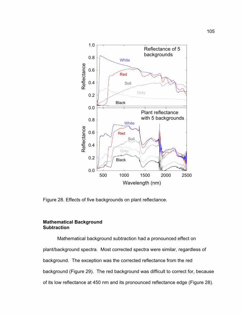
105
Ref
lect
ance
0.0
0.2
0.4
0.6
0.8
1.0
White
Soil
Gray
Black
Reflectance of 5backgrounds
Wavelength (nm)500 1000 1500 2000 2500
Ref
lect
ance
0.0
0.2
0.4
0.6
0.8Plant reflectance with 5 backgrounds
White
Soil
Gray
Black
Red
Red
Figure 28. Effects of five backgrounds on plant reflectance.
Mathematical Background Subtraction
Mathematical background subtraction had a pronounced effect on
plant/background spectra. Most corrected spectra were similar, regardless of
background. The exception was the corrected reflectance from the red
background (Figure 29). The red background was difficult to correct for, because
of its low reflectance at 450 nm and its pronounced reflectance edge (Figure 28).

106The mathematical subtraction method also tended to undercorrect for the
brightness component in some cases, resulting in higher overall corrected
reflectance values for plants with brightly colored backgrounds than for dark
backgrounds.
Therefore, use of SAVI after correction resulted in further improvement of
the correlation between spectral data and LAI (
Table 9). Correlation of all indices was improved with use of the
mathematical subtraction, although improvement of SAVI was most notable. Use
of a constant L value showed almost the same correlation after mathematical
correction as use of a custom L value.
Wavelength (nm)500 1000 1500 2000 2500
Ref
lect
ance
0.0
0.2
0.4
0.6
0.8
White Soil
GrayBlack
Red
Figure 29 Corrected spectra resulting from mathematical background subtraction.

107DISCUSSION
Vegetation Indices and Background Effects
In the absence of a soil-adjustment correction, the difference vegetation
index provides the highest correlation with LAI (r2 = 0.635) of any of the tested
indices. The primary reason for this high correlation is that difference vegetation
measurements are unaffected by the background offset. Therefore, the index is
affected only by the plant reflectance and the slope of reflectance of the
background between the wavelengths of interest. Backgrounds with gradual
slopes show only minor DVI variations based on background. However, DVI can
be sensitive to changes in solar angle and slight experimental error, so it should
be used with caution. DVI tends to be less accurate as an estimator of ground
cover during a growing season than are ratio indices in a normal field setting
(Table 4).
The other index with relatively high correlation was SAVI before
mathematic correction, although SAVI indices with best-fit L values showed
significantly higher correlation with LAI than did SAVI indices with the common L
value of 0.5 (0.576 and 0.549 vs. 0.266 and 0.289 for broadband and
narrowband SAVI, respectively (
Table 9).
108Mathematic Correction
Mathematical correction of background can decrease background effects
in spectral measurements. However, mathematical correction alone is often
insufficient to completely correct for the background. The most common cases
where this occurs involve a background with a reflectance shoulder. Of particular
concern are backgrounds with a region of high reflectance slope at a wavelength
higher than the reference wavelength. Correction of these backgrounds is
difficult and often erratic.
Correcting for a unique soil background is also more accurate if similar
wavelengths are used. The green NDVI performed well below the red NDVI and
other red indices for both uncorrected and corrected data.
The challenge of correcting for a soil background by subtracting the
background is that this requires a predetermined background reflectance. The
post processing also makes this method less user-friendly than most vegetation
indices. However, in cases where the background does not match standard soil
reflectance parameters, correction allows a more valid estimate of plant
parameters than uncorrected data.
REFERENCES
Demetriades-Shah, T.H., M.D. Steven, and J.A. Clark. 1990. High resolution derivative spectra in remote sensing. Remote Sens. Environ. 33:55-64.
Elvidge, C.D., and Z. Chen. 1995. Comparison of broad-band and narrow-band red and near-infrared vegetation indices. Remote Sens. Environ. 54:38-48.

109Hall, F.G., K.F. Huemmrich, and S.N. Goward. 1990. Use of narrow-band spectra
to estimate the fraction of absorbed photosynthetically active radiation. Remote Sens. Environ. 32:47-54.
Huete, A.R. 1988. A soil-adjusted vegetation index (SAVI). Remote Sens. Environ. 25:295-309.
Huete, A.R., D.F. Post, and R.D. Jackson. 1984. Soil spectral effects on 4-space vegetation discrimination. Remote Sens. Environ. 15:155-165.
Huete, A.R., R.D. Jackson, and D.F. Post. 1985. Spectral response of a plant canopy with different soil backgrounds. Remote Sens. Environ. 17:37-53.
Jackson, R.D., P.N. Slater, and P.J. Pinter. 1983. Discrimination of growth and water stress in wheat by various vegetation indices through clear and turbid atmospheres. Remote Sens. Environ. 13:187-208.
Kauth, R.J., and G.S. Thomas. 1976. The tasseled cap -- A graphic description of the spectral-temporal development of agricultural crops as seen by Landsat. Proceedings of the Symposium on Machine Processing of Remotely Sensed Data:41-51.
Peñuelas, J., J.A. Gamon, A.L. Fredeen, J. Merino, and C.B. Field. 1994. Reflectance indices associated with physiological changes in nitrogen- and water-limited sunflower leaves. Remote Sens. Environ. 48:135-146.
Sims, D.A., and J.A. Gamon. 2002. Relationships between leaf pigment content and spectral reflectance across a wide range of species, leaf structures and developmental stages. Remote Sens. Environ. 81:337-354.

110APPENDIX 4: SOLAR ANGLE AND VEGETATION INDICES
ABSTRACT
Plants and soil exhibit non-lambertian spectral characteristics and
specular reflectance properties. Spectral measurements are often performed
near solar noon to minimize the influence of solar angle on spectral indices.
However, plant stress indicators are not necessarily the most identifiable near the
middle of the day. For instance, excessive light changes short-term plant
photosynthetic activity, and water stress is most readily identifiable in the
afternoon as soil water deficit increases. Therefore, identification of plant
reflectance changes based on solar angle may be useful to determine stress at
angles other than near solar noon. This research was performed to quantify the
effects of solar angle on reflectance of a wheat canopy. Solar angle was found
to have a pronounced effect on plant canopy reflectance, and common
vegetation indices that correct for soil brightness were unable to correct for this
effect.
INTRODUCTION
Reflectance measurements are affected by both the angle of the sun and
the angle of the sensor from zenith (Figure 30), where zenith is a point normal to
the earth. Vegetated terrain exhibits strong forward and backscattering, which
varies by plant cover and type (Otterman et al., 1995). Satellite measurements
are predominantly conducted from the zenith or near the zenith, so many
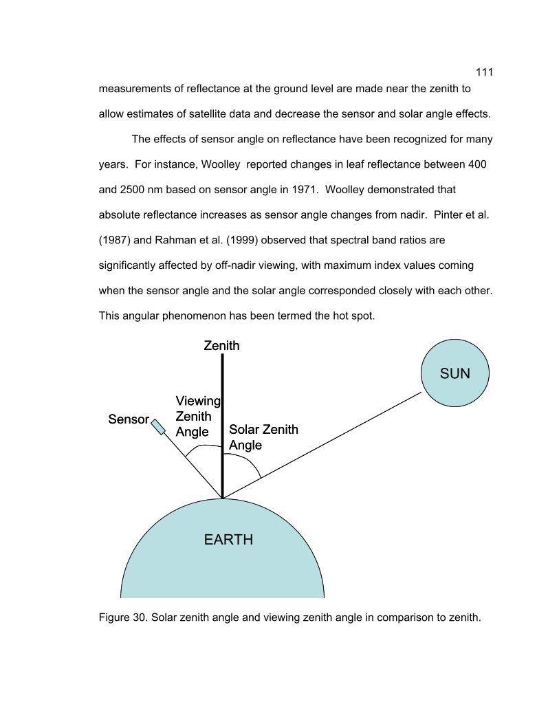
111measurements of reflectance at the ground level are made near the zenith to
allow estimates of satellite data and decrease the sensor and solar angle effects.
The effects of sensor angle on reflectance have been recognized for many
years. For instance, Woolley reported changes in leaf reflectance between 400
and 2500 nm based on sensor angle in 1971. Woolley demonstrated that
absolute reflectance increases as sensor angle changes from nadir. Pinter et al.
(1987) and Rahman et al. (1999) observed that spectral band ratios are
significantly affected by off-nadir viewing, with maximum index values coming
when the sensor angle and the solar angle corresponded closely with each other.
This angular phenomenon has been termed the hot spot.
SUN
Solar ZenithAngle
EARTH
SensorViewingZenithAngle
Zenith
SUN
Solar ZenithAngle
EARTH
SensorViewingZenithAngle
Zenith
Figure 30. Solar zenith angle and viewing zenith angle in comparison to zenith.
112Spectral studies are often performed near solar noon (the time of day that
the sun is closest to the zenith) to decrease the effects of solar angle on canopy
reflectance (Osborne et al., 2002; Otterman et al., 1995; Serrano et al., 2000).
However, the angle of the sun at solar noon is dependent on the day of the year.
Diurnal reflectance measurements of wheat canopies over the visible and NIR
regions of the spectrum suggest that visible reflectance remains roughly constant
throughout the day and infrared reflectance increases as angle from solar
azimuth increases. Asrar et al. (1985) observed that increased solar zenith angle
generally increased LAI estimates that used red and infrared spectral indices and
attributed these changes to increased infrared reflectance. Pinter et al. (1987)
reported that maxima in the NIR/red ratio were attained mid-morning and mid-
afternoon, and minima coincided with the high solar position near midday.
Rahman et al. (1999) also observed that reflectance amplitude varied with sensor
angle in relation to solar angle.
Solar position may also influence plant reflectance by influencing the
quantity and quality of light that are incident to the plant. For example, Gamon et
al. (1992) suggested that the xanthophyll chemical changes due to changes in
light intensity are partly responsible for changes in absorption efficiency and
changes in leaf reflectance between morning and afternoon. Antheraxanthin
undergoes deepoxidation to zeaxanthin under excessive photosynthetically
active radiation (PAR) and undergoes epoxidation under limiting PAR. The
concentrations of these component pigments are identifiable by reflectance
between 500 nm and 550 nm.

113Another physiological indicator of plant health is water concentration.
Water stress is usually identified best late in the afternoon, because high rates of
evapotranspiration increase leaf water deficit (Kramer, 1969). Therefore,
measurements at a non-optimal solar angle may provide useful estimates of
plant health.
MATERIALS AND METHODS
Spectral indices were tested for sensitivity to solar angle. Reflectance
measurements were performed on sixty-four wheat (Triticum aestivum cv.
Westbred 936) plots at 6:30 p.m. on May 29, 2002, and at 8:30 a.m., 10:15 a.m.,
12:15 p.m., and 3:30 p.m. on May 30, 2002 using a StellarNet EPP2000
spectrometer mounted in a wheelbarrow. All plots consisted of wheat at boot
stage. Atmospheric conditions were clear and cloudless for all measurements.
Solar angle was calculated from the following equation:
)15cos()cos()cos()sin()sin()sin( ψφφβ −×××−×= UTCtDD [9]
In this equation, ∃ is the solar angle, Ν is the latitude, D is the solar
declination, tUTC is the universal time correction, and ψ is the longitude. Latitude
was estimated as 41.78˚ N, longitude was estimated as 111.85˚, tUTC was
calculated as local daylight savings time plus 6 hours, and D was calculated as
21.83. Spectral indices were compared with 12:00 noon values.

114
NDVI at 65o Solar Angle0.0 0.2 0.4 0.6 0.8 1.0
ND
VI
0.0
0.2
0.4
0.6
0.8
1.0
1:1 line59o
25o
45o26o
RVI at 65o Solar Angle0 2 4 6 8 10 12
RV
I
02468
101214161820
59o
25o
45o
26o
Figure 31. NDVI and RVI by solar angle.

115
Wavelength (nm)400 500 600 700 800 900
Rat
io R
φ:R65
o
0.6
0.7
0.8
0.9
1.0
1.1
1.2
1.3
45o
26o
25o
59o
65o
Figure 32. Ratio of reflectance at lower solar angle to reflectance at 65o solar angle by wavelength. Points represent means of 16 plot readings.
0.2
0.4
0.6
0.8
1.0
1.2
1.4
1.6
500
600
700
800
900
0.3
0.4
0.50.6
0.70.8
0.9
Ref
lect
ance
Rat
io
Wavelength (nm)
Solar Angle Ratio
Figure 33. Comparison of reflectance ratio by wavelength with solar angle ratio to maximum solar angle. Lower solar angle resulted in increased ratio scatter, a
116general decrease of baseline reflectance, and an increase of reflectance peaks in the green and NIR regions.
RESULTS
Decreasing solar angle decreased baseline reflectance and increased
reflectance peaks at 550 nm and in the NIR. The 45˚ solar angle had a similar
reflectance baseline as reflectance measurements at lower solar angles (Figure
33). Spectral indices that attempt to remove soil background do not correct for
this feature, since it is wavelength dependent and follows vegetation patterns.
Therefore, spectral estimates of ground cover and greenness should be taken at
similar solar angle where possible.
Measurements at different solar angles showed differences in plant
reflectance at all wavelengths. Asrar et al. (1985) noted that both red and NIR
reflectance are affected by solar angle, but that NIR reflectance is less sensitive
to solar angle. This experiment confirms these results. However, sensitivity to
solar angle appears to be tied more to reflectance quantity at a wavelength than
to the wavelength itself.
REFERENCES
Asrar, G., E.T. Kanemasu, and M. Yoshida. 1985. Estimates of leaf area index from spectral reflectance of wheat under different cultural practices and solar angle. Remote Sens. Environ. 17:1-11.
Gamon, J.A., J. Penuelas, and C.B. Field. 1992. A narrow-waveband spectral index that tracks diurnal changes in photosynthetic efficiency. Remote Sens. Environ. 41:35-44.

117Kramer, P.J. 1969. Water stress and plant growth, p. 347-390 Plant and Soil
Water Relationships: A Modern Synthesis. McGraw-Hill, New York.
Osborne, S.L., J.S. Schepers, D.D. Francis, and M.R. Schlemmer. 2002. Use of spectral radiance to estimate in-season biomass and grain yield in nitrogen- and water-stressed corn. Crop Sci. 42:165-171.
Otterman, J., T. Brakke, and J. Smith. 1995. Effects of leaf-transmittance versus leaf-reflectance on bi-directional scattering from canopy/soil surface: an analytical study. Remote Sens. Environ. 54:49-60.
Pinter, P.J., G. Zipoli, G. Maracchi, and R.J. Reginato. 1987. Influence of topography and sensor view angles on NIR/red ratio and greenness vegetation indices of wheat. Int. J. Remote Sens. 8:953-957.
Rahman, H., D.A. Quadir, A.Z.M.Z. Islam, and S. Dutta. 1999. Wiewing angle effect on the remote sensing monitoring of wheat and rice crops. Geocarto International 14:75-79.
Serrano, L., I. Filella, and J. Penuelas. 2000. Remote sensing of biomass and yield of winter wheat under different nitrogen supplies. Crop Sci. 40:723-731.
Woolley, J.T. 1971. Reflectance and transmittance of light by leaves. Plant Physiol. 47:656-662.

118APPENDIX 5: GRAPHS AND STATISTICS FOR NITROGEN AND WATER-
STRESS PAPER
COMPARISON OF THE UNSTRESSED LINE AMONG TREATMENTS
Res
idua
l Fro
mU
nstre
ssed
Lin
e
-0.08
-0.06
-0.04
-0.02
0.00
0.02
0.04
Res
idua
l Fro
mU
nstre
ssed
Lin
e
-0.08
-0.06
-0.04
-0.02
0.00
0.02
Res
idua
l Fro
mU
nstre
ssed
Lin
e
-0.08-0.06-0.04-0.020.000.020.040.060.08
Days After Planting30 40 50 60 70 80 90
Res
idua
l Fro
mU
nstre
ssed
Lin
e
-0.08-0.06-0.04-0.020.000.020.040.060.08
UnstressedVery H2O N stressed
H2O N stressed
N stress
Unstressedb
Very H20 stressed
Unstressed
Very H2Ostressed
Unstressed
2002a
b
c
d
N stress
Unstresseda
Less H2O stressed
N stressed
Figure 34. Comparison of the residuals of all treatments from the unstressed line during 2002. Graph a compares the unstressed treatment to nitrogen-stressed treatments with varying levels of water stress. Graph b compares the unstressed plots nearest the line source with those that were further from the line source. Graph c compares the unstressed treatment with two levels of water stress. Graph d compares the unstressed treatment with nitrogen-stressed plots and very water-stressed plots. All error bars represent ± 1 standard deviation from the mean by date.

119Figure 34 demonstrates the predictive power of the unstressed line during
the growing season for all treatments in the 2002 study. Graph a in this figure
compares the effect of water-stress on nitrogen-stressed plots during the growing
season. A heavy water stress increases the GNDVI:NDVI ratio significantly,
which in turn makes the residual from the unstressed line more positive. This
attribute is shown to a lesser extent in cases of less water stress.
Graph b compares the effects of proximity to the line source on changes in
spectral attributes of plots. It was suggested that plots closest to the line source
will be over-watered, and that the resultant leaching of nutrients will result in mild
nitrogen-deficiency. These results suggest that if any such stress did occur, it
was too mild to be detected by this method. This suggestion is supported by the
SPAD data for these treatments during the growing season (Figure 35). The
plots showed similar, and usually overlapping, SPAD values throughout the
growing season, suggesting that the placement of the unstressed plots did not
significantly affect plant nitrogen status for this study.
Graph c of Figure 34 compares the effects of two levels of water stress on
the average residual from the unstressed line. The very water-stressed plots had
a higher residual at the end of the season than the less water-stressed plots,
which in turn had a higher residual than the unstressed plots. This pattern of
increasing residual with increasing water stress follows the same pattern as with
the nitrogen-stressed plots (graph a). Graph d shows the broad separation
between nitrogen-stress, water-stress, and control plots by the end of the season
based on the unstressed line.

120
Days After Planting30 40 50 60 70 80
Ave
rage
SP
AD
Val
ues
25
30
35
40
45
50
55
60Unstressed Plots Closest to the Line Source
N-Stressed PlotsClosest to the Line SourceOther N-StressedPlots
2002
Other UnstressedPlots
Figure 35. Comparison of the SPAD values of unstressed and N-stressed plots closest to the line source compared to other unstressed and N-stressed plots plots. Plots showed similar, and usually overlapping, SPAD values throughout the growing season. This suggests that the placement of the unstressed plots did not significantly affect plant nitrogen status for either treatment due to leaching. Error bars represent ± 1 standard deviation from the mean by date.
The following is the derivation of the conversion of the normalized green:red
relationship (NGR) from an NDVI relationship to a DVI relationship.
green
red
DVIDVI
RNIRGNIRGNIRRNIR
GNIRGNIR
RNIRRNIR
~)()()()(
)()(
)()(
+×−+×−
=
+−
+−

121STATISTICAL TEST OF 2001 AND 2002 UNSTRESSED LINES
The test statistic ((slope a - slope b) - 0)/(variance of slope a) = t (degrees of
freedom of slope a), as described by Neter et al. (1996), was performed to determine if
the 2001 and 2002 regression lines were statistically different. In this case, the
degrees of freedom of the slope is determined as n-2, with n being the number of
sample points that the regression is fitted to. The null hypothesis in this case is
that the slope of line 1 (a) is not different than the slope of line 2 (b). The
following table includes the parameters for both the 2001 and 2002 regression
lines and the results. Tests of both lines reveal P-values greater than 0.05, and
we cannot reject the null hypothesis that the lines are not statistically different.
Table 10. Statistical parameters of the 2001 and 2002 regression equations used to estimate whether the slopes are different.
Year Regression Line
Slope Standard Error of Slope
Degrees of Freedom
t value Test of Significance
2001 GNDVI = 0.67 x NDVI + 0.17
0.67 0.613 57 0.075 P>0.4
2002 GNDVI = 0.70 x NDVI + 0.14
0.70 0.095 513 0.486 P>0.3
REFERENCE
Neter, J., M.H. Kutner, C.J. Nachtsheim, and W. Wasserman. 1996. Applied linear statistical models. 4th ed. Irwin, Chicago.

122 APPENDIX 6: GRAPHS OF DVI, RVI, NDVI, AND GNDVI COMPARED WITH
DIGITAL IMAGES OF GROUND COVER
Image Ground Cover (%)0 20 40 60 80
0.0
0.2
0.4
0.6
0.8
0.0
0.1
0.2
0.3
0.4
0.5
0.6
r2=0.90
r2=0.82
0.0
0.2
0.4
0.6
0.8
1.0
r2=0.88
0 20 40 60 80 1000
2
4
6
8
10
12
r2=0.88
NDVI
RVI
GNDVI
DVI
Figure 36. Comparison of DVI, NDVI, GNDVI, and RVI with digital images of ground cover. DVI had a lower correlation with ground cover than the ratio indices. RVI had a similar correlation with ground cover as NDVI, but the relationship was nonlinear. NDVI and GNDVI both had a high linear correlation with ground cover.


![Monitering And Yield Estimation of Sugarcane Using Remote ... · and crop yield [10–12]. The NDVI value, which is a vegetative index that compares reflectance at the red and near](https://img.dokumen.tips/doc/110x75/5f0304367e708231d4071fad/monitering-and-yield-estimation-of-sugarcane-using-remote-and-crop-yield-10a12.jpg)