Embed Size (px)
Citation preview
Anatomy of the Trade Collapse, Recovery, andSlowdown: Evidence from Korea
Sooyoung Lee∗
Korea Institute for International Economic Policy
May 2017
AbstractThe last decade of the world trade has been marked by an unprecedented collapse, quick
recovery, slowdown, another drop, and recovery. To study cyclical and structural aspectsof the recent trend of trade, I use both aggregate and disaggregated trade statistics of asmall open economy, South Korea, whose economic success and growth have been heavilydependent on exports. The aggregate trend of the country is surprisingly similar to thatof the world, which is why the trend of Korea’s export is called a proxy for the world. Ishow that while the last drop of trade after 2015 has cyclical aspects, there is evidencethat the continued slowdown from 2012 is structural: (1) the so-called ‘China factor’ isfound in the analysis of trade-income elasticity of the world and China for imports fromKorea. (2) The bilateral trade barriers between Korea and its important trading partnersare universally tightening. I also show that the firm sizes, destination countries, and the modeof transactions affect disaggregated trade flows during the slowdown periods. It is advisableto diversify main export products to lower the effect of oil prices on export prices and tostrengthen the cooperation with ASEAN countries, whose trade barriers have exceptionallydiminished throughout the last decade.
Keywords: the Great Trade Collapse, trade slowdown, trade elasticity, trade barriers,Korea
JEL Classification Numbers: F14, O24
1
1 Introduction
In the last decade, the world trade has experienced an unprecedented collapse, remarkable
recovery, and persistent slowdown. At the end of the slowdown, the world trade entered
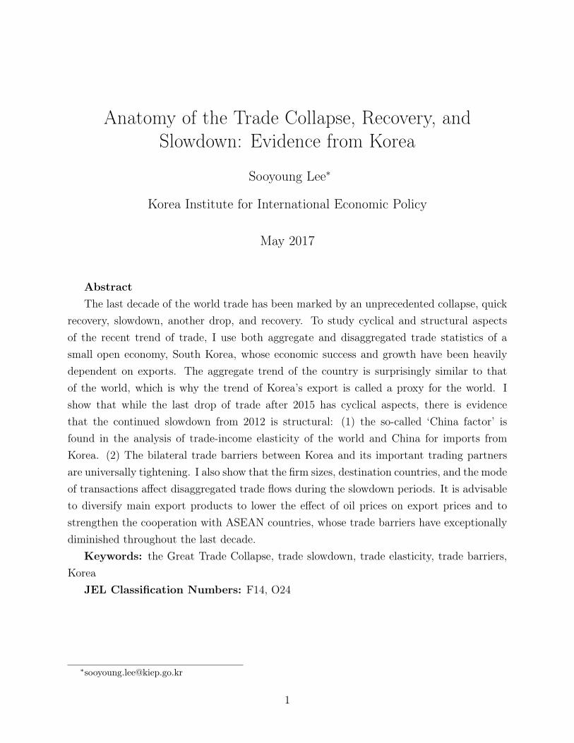
another period of negative growth rates, which finally turned positive in late 2016. Figure 1
presents the level and growth rate of exports for the world, South Korea, and its two largest
trading parters, China and the US, in the last decade. The trends of aggregate exports across
the three countries are similar to that of the world.1 The trends show distinct phases, which
are quite different from the long monotonic increase before the financial crisis of 2008-09.
The dynamic behaviors of international trade in the last decade worry policy makers and
intrigue trade economists for its cause.2 In this paper, I focus on the recent trade collapse,
recovery, and prolonged slowdown to shed light on the discussions about whether the current
slowdown is structural or cyclical. I use detailed trade statistics of a small open economy,
South Korea, whose economic success and growth have been heavily dependent on exports. I
present evidence that although the current drop of trade has cyclical aspects, the continued
slowdown from 2012 has structural aspects. I also show that the destination countries, firm
sizes, and organization of firms matter for the detailed aspects of trade slowdown and drop.
I attempt to answer the following questions in this paper. The first question is about
whether the current trade slowdown is structural or cyclical. While there are studies on this
topic as in Hoekman (2015) and Constantinescu et al. (2015), detailed studies at a country
level regarding the trade slowdown are rare as of now. To answer this question, I use the
following methods. First, I analyze the relationship between oil prices and export prices of
Korea, to see their cyclical effect on export volumes. I decompose the trade growth into the
extensive margin (the sum of entry and exit effect) and the intensive margin (the sum of
quantity and price effects) and observe the effect of prices over time. Second, I estimate the
1However, the exports volume of China looks different from Korea and the US because of China’s morepronounced seasonality. Historically, in China, exports of first quarter tend to be lower than other quarters,but China’s trend of quarter-on-quarter export growth rate is similar to the world’s export growth rate.Vietnam exhibits a similar type of seasonality in its export statistics.
2See Bems et al. (2010), Levchenko et al. (2010), or Baldwin (2009), for example.
2

Figure 1: The export trends in the last decade
-40
-20
020
40%
2.5
33.
54
4.5
5Tr
illio
n U
SD
2007q3 2009q3 2011q3 2013q3 2015q3
World
-40
-20
020
40%
8010
012
014
016
0B
illio
n U
SD
2007q3 2009q3 2011q3 2013q3 2015q3
Korea
-40
-20
020
40%
200
300
400
500
600
700
Bill
ion
US
D
2007q3 2009q3 2011q3 2013q3 2015q3
China
-30
-20
-10
010
20%
250
300
350
400
450
Bill
ion
US
D
2007q3 2009q3 2011q3 2013q3 2015q3
US
Aggregate export Export growth rate
Sources: IMF Direction of Trade Statistics (http://www.imf.org/en/Data, ac-cessed on January 1, 2017).Note: Own calculation of the author. The left axis is the level of exports inUSD, and the right axis is the quarter-on-quarter growth rate of exports.
trade-income elasticities focusing on the world’s import demand, separately for goods from
the world and from Korea. To address the serial correlations between the world trade and
income statistics, I employ the error correction model. Third, I estimate the tariff-equivalent
bilateral trade barriers between Korea and its important trading partners. If the discussions
about the new protectionism by scholars and policy makers have actual substance, the trend
of trade barriers should be increasing.3
The second question I pose is regarding the heterogeneous trade flows at a disaggregate
level. I expect that, although the overall export has its distinct trend in each period, which I
discuss more in detail in the next section, firm sizes, destination countries, and organization
of firms affect trade flows at the disaggregated level. The literature reports that, during the
3See Evenett and Fritz (2015), for details.
3
Great Trade Collapse, the negative shock originated from the developed countries and spread
through the global values chains (Eaton et al., 2016; Bussière et al., 2013). I compare the
drop of goods exports in slowdown and trade collapse, which are the two unusual periods in
the recent history when world trade has substantially dropped altogether. (Korea’s annual
exports dropped by 20.9 percent during the collapse and 9.5 percent during the 2015 drop.)
Destination countries matter if the trade collapse originated from advanced countries and
the trade slowdown is due to the weak growth of emerging countries as UNCTAD (2016)
reports. Also, Bernard et al. (2009) show that intrafirm trade stayed resilient during the
1997 Asian financial crisis. I check whether Korea’s intrafirm trade stayed resilient during
the last decade as well. Since the Korean intrafirm trade statistics is inaccessible by policy,
I combine the US related-party trade statistics with Korean exports statistics to observe the
intrafirm flows between Korea and the US.
Results show that, since 2012, exceptionally low oil prices drove down export prices and
the value of exports started diverging from the quantity of exports, which showed steady
growth. The decomposition results indicate that the price effect is statistically significant
only in 2015. Thus, the trade drop in the last two years largely stems from the price effects.
The overall slowdown of trade, which started from 2012, however, seems to have structural
aspects. The world’s long-run income elasticity of imports from the world fell from 2.4 before
the global crisis to 1.1 after the crisis. The world’s long run elasticity of imports from Korea
also fell from 2.2 to 1.1. Also, the bilateral trade barriers between Korea and its important
trading partners have universally increased since 2012. So although the trade drop in 2015
appears to be temporary, the structural slowdown of world trade started from 2012, and
Korea’s sluggish exports in 2012-16 are in line with this world trend.
Regarding the heterogeneous trade flows, I first find that large corporations are more
resilient to both the trade collapse in 2008 and trade drop in 2015. Large firms’ exports
to emerging countries, however, fell relatively more in 2015 than in 2009 while small firms’
exports to emerging countries fell relatively less in 2015 than in 2009. Large firms’ exports to
4
emerging countries fell 5 percentage point more in 2015 compared to 2009, mostly because of
weak intermediate goods exports. Small firms’ exports to emerging countries fell 7 percentage
point less in 2015 compared to 2009. Korea’s intrafirm exports to the US deeply dropped
in but also quickly recovered from the Great Trade Collapse. Intrafirm exports fell by 47
percent in 2009 but recovered by 55 percent in 2010, while arm’s length trade fell by 8.3
percent in 2009 and recovered by 0.6 percent in 2010. Intrafirm trade stayed more stable
during the trade slowdown. When I decompose the intrafirm exports’ growth rate into the
quantity, price, entry, and exit effects, all of them stayed far more stable than those of arm’s
length exports throughout the last decade.
This paper contributes to the debate regarding whether the current trade slowdown is
structural or cyclical. I provide two pieces of concrete evidence that the export drop in 2015
stems from low oil prices: one is the divergence of Korean export value index from its export
quantity index, which started from late 2014 when oil prices plunged. The export prices fell
so much that while export quantity index was growing, export value index was diminishing.
The other evidence is the decomposition results that price effect is significant only in 2015.
Therefore, the drop of trade in 2015 looks largely cyclical. While trade slowdown is widely
discussed in the literature, this paper is the first one to specifically discuss the trade drop in
2015 and its causes to the best of my knowledge.
I also contribute to the literature by providing evidence that the slowdown of trade from
2012 has structural aspects. I identify the so-called “China factor” in the drop of trade-
income elasticity after the global financial crisis, by showing that the pattern of the world’s
trade-income elasticity for imports from Korea (as well as for imports from the world) is
similar to that of China. At the same time, there is evidence that Korea’s trade barriers
with important trading partners are steadily increasing after 2012. Trade barriers have been
increasing as protectionism measures toward Korea’s export products are steeply increasing
after the global financial crisis.4
4According to the Korea International Trade Association (http://ntb.kita.net), the number of protec-tionism measures including anti-dumping, safeguards, and countervailing duties toward Korean products has
5
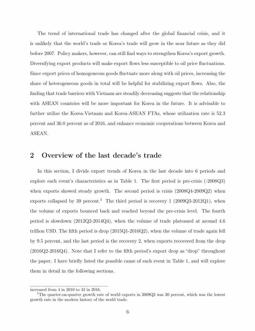
The trend of international trade has changed after the global financial crisis, and it
is unlikely that the world’s trade or Korea’s trade will grow in the near future as they did
before 2007. Policy makers, however, can still find ways to strengthen Korea’s export growth.
Diversifying export products will make export flows less susceptible to oil price fluctuations.
Since export prices of homogeneous goods fluctuate more along with oil prices, increasing the
share of heterogeneous goods in total will be helpful for stabilizing export flows. Also, the
finding that trade barriers with Vietnam are steadily decreasing suggests that the relationship
with ASEAN countries will be more important for Korea in the future. It is advisable to
further utilize the Korea-Vietnam and Korea-ASEAN FTAs, whose utilization rate is 52.3
percent and 36.0 percent as of 2016, and enhance economic cooperations between Korea and
ASEAN.
2 Overview of the last decade’s trade
In this section, I divide export trends of Korea in the last decade into 6 periods and
explore each event’s characteristics as in Table 1. The first period is pre-crisis (-2008Q3)
when exports showed steady growth. The second period is crisis (2008Q4-2009Q2) when
exports collapsed by 39 percent.5 The third period is recovery 1 (2009Q3-2012Q1), when
the volume of exports bounced back and reached beyond the pre-crisis level. The fourth
period is slowdown (2012Q2-2014Q4), when the volume of trade plateaued at around 4.6
trillion USD. The fifth period is drop (2015Q1-2016Q2), when the volume of trade again fell
by 9.5 percent, and the last period is the recovery 2, when exports recovered from the drop
(2016Q2-2016Q4). Note that I refer to the fifth period’s export drop as “drop” throughout
the paper. I have briefly listed the possible cause of each event in Table 1, and will explore
them in detail in the following sections.
increased from 4 in 2010 to 42 in 2016.5The quarter-on-quarter growth rate of world exports in 2009Q2 was 30 percent, which was the lowest
growth rate in the modern history of the world trade.
6
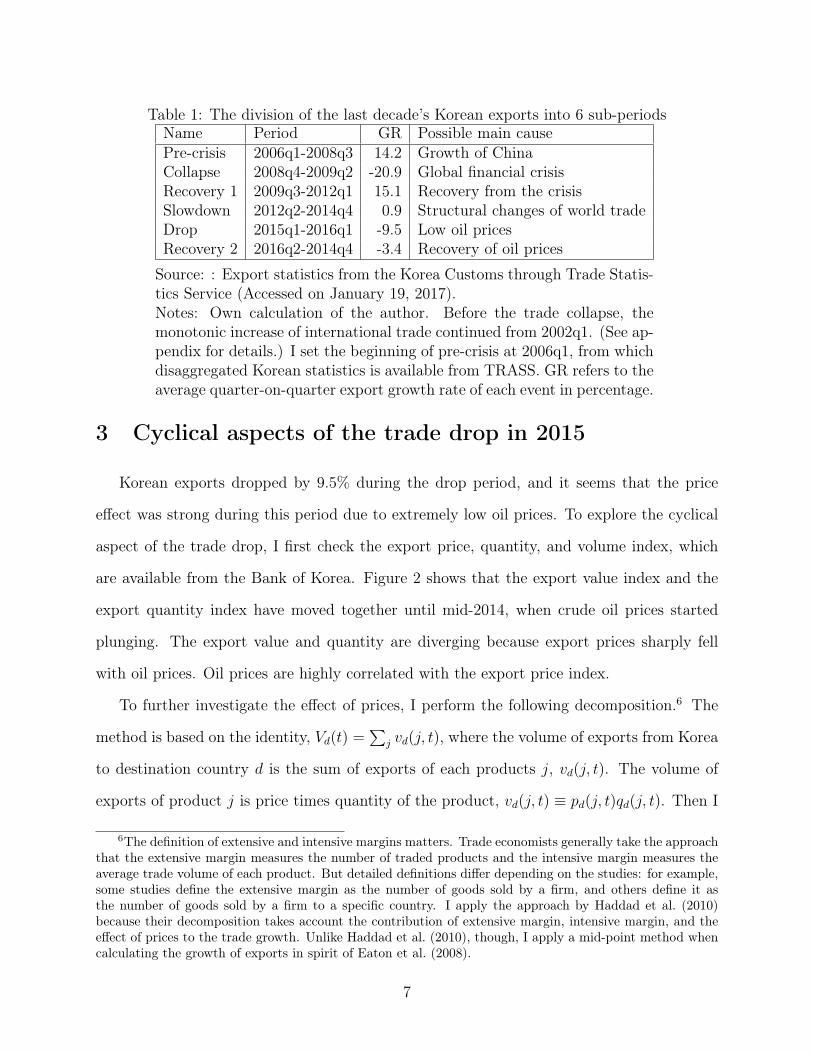
Table 1: The division of the last decade’s Korean exports into 6 sub-periodsName Period GR Possible main causePre-crisis 2006q1-2008q3 14.2 Growth of ChinaCollapse 2008q4-2009q2 -20.9 Global financial crisisRecovery 1 2009q3-2012q1 15.1 Recovery from the crisisSlowdown 2012q2-2014q4 0.9 Structural changes of world tradeDrop 2015q1-2016q1 -9.5 Low oil pricesRecovery 2 2016q2-2014q4 -3.4 Recovery of oil prices
Source: : Export statistics from the Korea Customs through Trade Statis-tics Service (Accessed on January 19, 2017).Notes: Own calculation of the author. Before the trade collapse, themonotonic increase of international trade continued from 2002q1. (See ap-pendix for details.) I set the beginning of pre-crisis at 2006q1, from whichdisaggregated Korean statistics is available from TRASS. GR refers to theaverage quarter-on-quarter export growth rate of each event in percentage.
3 Cyclical aspects of the trade drop in 2015
Korean exports dropped by 9.5% during the drop period, and it seems that the price
effect was strong during this period due to extremely low oil prices. To explore the cyclical
aspect of the trade drop, I first check the export price, quantity, and volume index, which
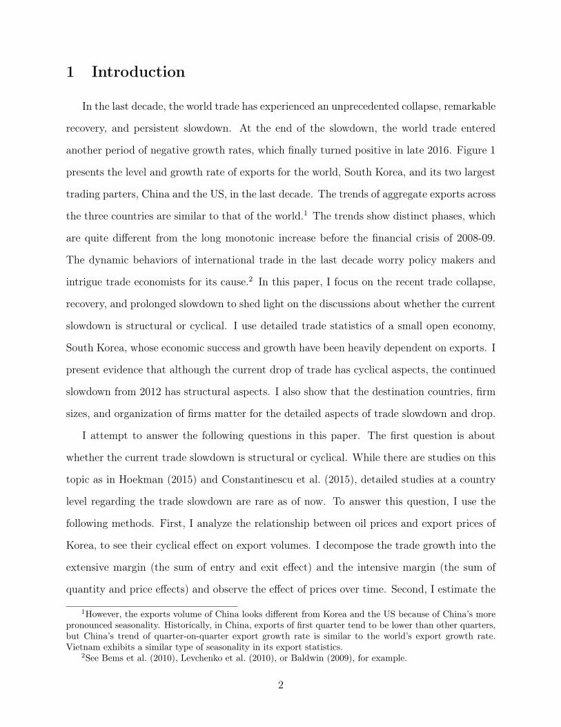
are available from the Bank of Korea. Figure 2 shows that the export value index and the
export quantity index have moved together until mid-2014, when crude oil prices started
plunging. The export value and quantity are diverging because export prices sharply fell
with oil prices. Oil prices are highly correlated with the export price index.
To further investigate the effect of prices, I perform the following decomposition.6 The
method is based on the identity, Vd(t) =∑
j vd(j, t), where the volume of exports from Korea
to destination country d is the sum of exports of each products j, vd(j, t). The volume of
exports of product j is price times quantity of the product, vd(j, t) ≡ pd(j, t)qd(j, t). Then I
6The definition of extensive and intensive margins matters. Trade economists generally take the approachthat the extensive margin measures the number of traded products and the intensive margin measures theaverage trade volume of each product. But detailed definitions differ depending on the studies: for example,some studies define the extensive margin as the number of goods sold by a firm, and others define it asthe number of goods sold by a firm to a specific country. I apply the approach by Haddad et al. (2010)because their decomposition takes account the contribution of extensive margin, intensive margin, and theeffect of prices to the trade growth. Unlike Haddad et al. (2010), though, I apply a mid-point method whencalculating the growth of exports in spirit of Eaton et al. (2008).
7
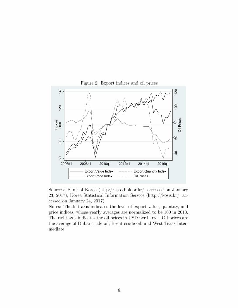
Figure 2: Export indices and oil prices
4060
8010
012
0O
il P
rices
6080
100
120
140
Indi
ces
2006q1 2008q1 2010q1 2012q1 2014q1 2016q1
Export Value Index Export Quantity IndexExport Price Index Oil Prices
Sources: Bank of Korea (http://ecos.bok.or.kr/, accessed on January23, 2017), Korea Statistical Information Service (http://kosis.kr/, ac-cessed on January 24, 2017).Notes: The left axis indicates the level of export value, quantity, andprice indices, whose yearly averages are normalized to be 100 in 2010.The right axis indicates the oil prices in USD per barrel. Oil prices arethe average of Dubai crude oil, Brent crude oil, and West Texas Inter-mediate.
8
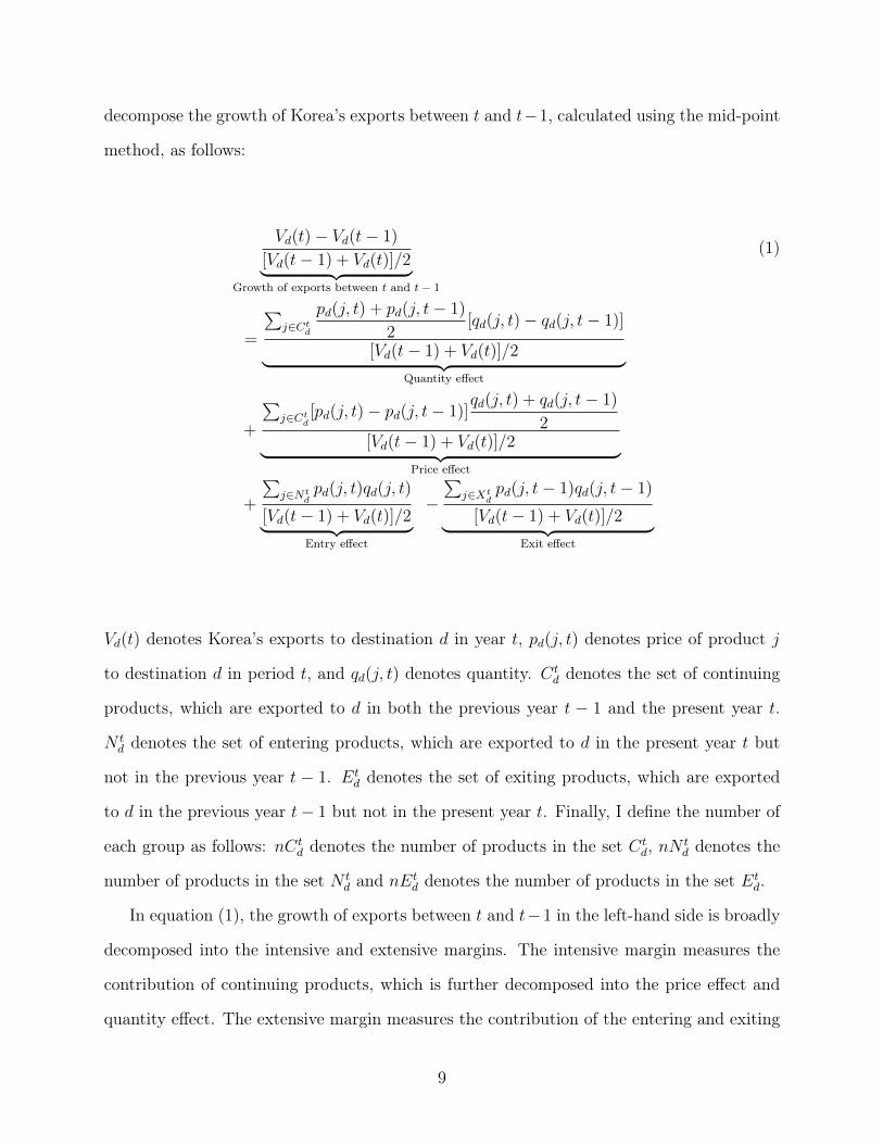
decompose the growth of Korea’s exports between t and t−1, calculated using the mid-point
method, as follows:
Vd(t)− Vd(t− 1)
[Vd(t− 1) + Vd(t)]/2︸ ︷︷ ︸Growth of exports between t and t− 1
(1)
=
∑j∈Ct
d
pd(j, t) + pd(j, t− 1)
2[qd(j, t)− qd(j, t− 1)]
[Vd(t− 1) + Vd(t)]/2︸ ︷︷ ︸Quantity effect
+
∑j∈Ct
d[pd(j, t)− pd(j, t− 1)]
qd(j, t) + qd(j, t− 1)
2[Vd(t− 1) + Vd(t)]/2︸ ︷︷ ︸
Price effect
+
∑j∈Nt
dpd(j, t)qd(j, t)
[Vd(t− 1) + Vd(t)]/2︸ ︷︷ ︸Entry effect
−∑
j∈Xtdpd(j, t− 1)qd(j, t− 1)
[Vd(t− 1) + Vd(t)]/2︸ ︷︷ ︸Exit effect
Vd(t) denotes Korea’s exports to destination d in year t, pd(j, t) denotes price of product j
to destination d in period t, and qd(j, t) denotes quantity. Ctd denotes the set of continuing
products, which are exported to d in both the previous year t − 1 and the present year t.
N td denotes the set of entering products, which are exported to d in the present year t but
not in the previous year t − 1. Etd denotes the set of exiting products, which are exported
to d in the previous year t− 1 but not in the present year t. Finally, I define the number of
each group as follows: nCtd denotes the number of products in the set Ct
d, nN td denotes the
number of products in the set N td and nEt
d denotes the number of products in the set Etd.
In equation (1), the growth of exports between t and t−1 in the left-hand side is broadly
decomposed into the intensive and extensive margins. The intensive margin measures the
contribution of continuing products, which is further decomposed into the price effect and
quantity effect. The extensive margin measures the contribution of the entering and exiting
9

products. Therefore, the growth of exports in the left-hand side is decomposed into the
quantity effect, price effect, entry effect, and exit effect.
I use a disaggregated Korean exports data from the Trade Statistics Service, which collects
all exports and imports information from the Korean Customs. The export statistics use the
Korean Harmonized System at the 10-digit level, but, for better concordances, I aggregate
them into HS 6-digit, which comprises 4,386 products. Since there was a revision of the
Harmonized System in 2012, I convert the 2012 system to 2007 using the concordance table
from the United Nation Statistics Divisions.
Table 2: The numbers of continuing, entry, and exit groupYear Continuing Entry Exit
mean SD mean SD mean SD2006-2007 260.1 466.9 116.9 128.0 96.0 102.02007-2008 286.3 497.0 109.5 113.3 94.0 96.92008-2009 287.0 498.2 108.3 112.0 103.7 108.52009-2010 294.3 509.2 117.1 122.2 95.8 97.12010-2011 308.6 525.3 114.0 117.6 101.1 105.22011-2012 317.6 535.3 113.6 115.0 101.4 102.82012-2013 330.6 550.9 120.4 120.4 100.6 99.32013-2014 345.4 561.7 124.2 120.9 105.7 102.62014-2015 353.9 570.0 115.6 111.5 115.7 110.42015-2016 353.9 574.8 120.9 118.2 113.6 109.8
Source: Export statistics from the Korea Customs throughTrade Statistics Service (Accessed on January 19, 2017).Notes: Own calculation of the author. Each row reports themean and standard deviation of the number of continuing(nCt
d), entry (nN td), and exit (nEt
d) group across countries.
Once the decomposition is complete, I get the growth rate of the exports from the previous
year and its decomposition into the four effects for each country and each year. For each year,
I regress the growth rate by each margin. Since equation (1) is an identity, the coefficients
have the following equality in each year: (quantity effect)+(price effect)+(entry effect)-(exit
effect)=1.7 Each coefficient shows the percentage contribution of each effect.
Table 2 lists the average and standard deviation of products in continuing, entry, and exit
groups. The sample years range from 2007 to 2016. The number of products in continuing7The regression method is similar to Osnago and Tan (2016).
10

Table 3: OLS results - Effect of margins on export growthYear Quantity Price Entry Exit N. of Observations
Regressions Base2006-2016 0.189** 0.0113 0.442*** -0.356*** 241 242,324
(0.0855) (0.0780) (0.0279) (0.0342)2006-2007 0.269*** -0.0215 0.338*** -0.415*** 230 210,500
(0.0549) (0.0287) (0.0521) (0.0502)2007-2008 0.338*** -0.0469 0.348*** -0.361*** 228 222,021
(0.0826) (0.0474) (0.0587) (0.0623)2008-2009 0.294*** -0.0388 0.419*** -0.299*** 231 230,476
(0.0475) (0.0246) (0.0467) (0.0480)2009-2010 0.234*** -0.0380 0.360*** -0.415*** 234 237,773
(0.0475) (0.0246) (0.0531) (0.0509)2010-2011 0.164*** 0.0123 0.430*** -0.394*** 235 246,035
(0.0320) (0.0165) (0.0542) (0.0476)2011-2012 0.258*** -0.0245 0.361*** -0.404*** 237 252,796
(0.0515) (0.0295) (0.0532) (0.0563)2012-2013 0.232*** -0.0382 0.496*** -0.311*** 237 261,637
(0.0505) (0.0284) (0.0577) (0.0531)2013-2014 0.432*** -0.123 0.300*** -0.391*** 237 273,101
(0.111) (0.0770) (0.0518) (0.0630)2014-2015 0.405*** -0.166** 0.413*** -0.347*** 237 277,610
(0.100) (0.0842) (0.0508) (0.0582)2015-2016 0.0407 0.180 0.489*** -0.289*** 238 278,633
(0.202) (0.192) (0.0522) (0.0524)
Source: Export statistics from the Korea Customs through Trade Statistics Ser-vice (Accessed on January 19, 2017)Note: Own calculation of the author. The independent variable is the growth rateby country, [Vd(t)−Vd(t− 1)]/[(Vd(t− 1)+Vd(t))/2], in all cells. Robust standarderrors in parentheses. *** p<0.01, ** p<0.05, * p<0.1.
group has plateaued between 2015-16, while that in entry (exit) group slightly increased
(decreased). Table 3 presents the results of the decomposition. The four effects are from the
decomposition of the growth rate of the present year from the previous year. The number of
observations for regressions ranges from 228 to 241, which is equal to the number of Korea’s
export destination countries. The number of observations of the base dataset ranges between
210,500 to 278,633. The base dataset for each year contains the non-zero export flows at the
HS 6-digit product, country, and (the current and previous) year.
The first row of Table 3 exhibits the decomposition results of export growth between 2006
and 2016: quantity effect contributed 19 percent of the growth and price effect contributed
11
1 percent, which means that the effect of the intensive margin contributed 20 percent to the
growth between 2006 and 2016. The contribution of the extensive margin is 80 percent. The
smaller contribution of intensive margin compared to extensive margin is due to the fact
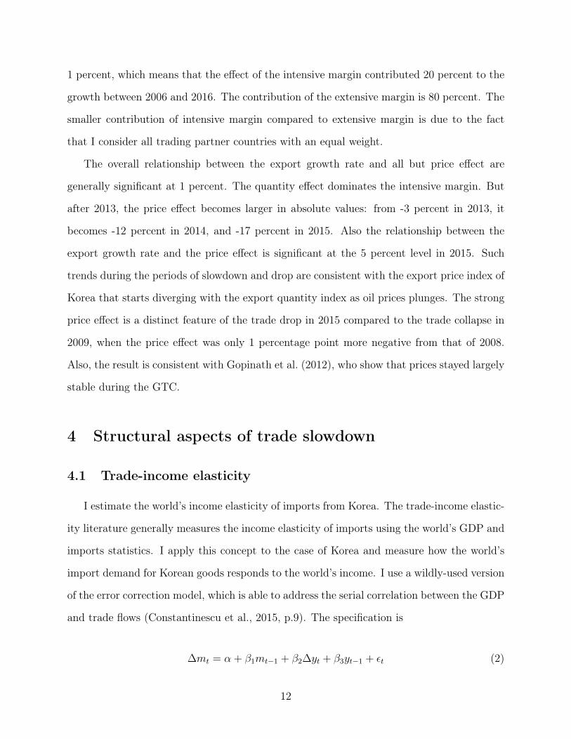
that I consider all trading partner countries with an equal weight.
The overall relationship between the export growth rate and all but price effect are
generally significant at 1 percent. The quantity effect dominates the intensive margin. But
after 2013, the price effect becomes larger in absolute values: from -3 percent in 2013, it
becomes -12 percent in 2014, and -17 percent in 2015. Also the relationship between the
export growth rate and the price effect is significant at the 5 percent level in 2015. Such
trends during the periods of slowdown and drop are consistent with the export price index of
Korea that starts diverging with the export quantity index as oil prices plunges. The strong
price effect is a distinct feature of the trade drop in 2015 compared to the trade collapse in
2009, when the price effect was only 1 percentage point more negative from that of 2008.
Also, the result is consistent with Gopinath et al. (2012), who show that prices stayed largely
stable during the GTC.
4 Structural aspects of trade slowdown
4.1 Trade-income elasticity
I estimate the world’s income elasticity of imports from Korea. The trade-income elastic-
ity literature generally measures the income elasticity of imports using the world’s GDP and
imports statistics. I apply this concept to the case of Korea and measure how the world’s
import demand for Korean goods responds to the world’s income. I use a wildly-used version
of the error correction model, which is able to address the serial correlation between the GDP
and trade flows (Constantinescu et al., 2015, p.9). The specification is
∆mt = α + β1mt−1 + β2∆yt + β3yt−1 + εt (2)
12

where α is a constant, mt is the log of world’s import from Korea (or Korean exports to the
world) in time t, yt is the log of world’s income (GDP) at time t, ∆ denotes first differences.
The model is based on the simple relationship of trade and GDP, Mt = QYt, where imports
(Mt) is a proportion (a constant Q) of GDP (Yt). Some algebra show that, in equation (2),
β2 is the short run trade elasticity, −β3/β1 is the long run trade elasticity, and β1 is the
speed of adjustment of import to GDP, or the error correction term.8
I use quarterly statistics of trade from IMF DOTS and GDP from Bloomberg to run the
error correction model in equation (2). Since I give special attention to how the long-run
trade-income elasticities are shifting before and after the global financial crisis, I divide the
total time periods into 2000q1-2008q4 and 2010q1-2016q2. In addition to the world’s income,
I calculate the sensitivity of trade with respect to incomes and imports of China, the US,
and the European Union. For each economy, I separate the elasticity with respect to imports
from Korea and imports from the world.
Table 4 presents the estimation results of the error correction model when considering
how the imports from Korea and the imports from the world respond to the changes of the
importing party’s income in the cases of the world, China, US, and EU. Panel A presents
the case when the importing party is the world, and the first three columns of Panel A show
how the world’s imports from Korea respond to the world’s income for 2000-2016, before
crisis and after the crisis.
I analyze the results mainly in two aspects: the change in the significance of the beta
coefficients, β1, β2, and β3, and the change in the level of the long-run elasticity. If the
relationship between trade and income gets weaker after the global financial crisis, I would
observe either statistically insignificant coefficients or significant but lower implied long-run
elasticity. In Panel A, the long-run trade-income elasticity of the world for imports from
Korea became weaker after the global financial crisis. In the second column of panel A, all
three beta coefficients are statistically significant at 1 percent and the long-run elasticity is
8See Escaith et al. (2010), pp.23-24 for the detailed derivation of the short-run and long-run tradeelasticity from the simple relationship, Mt = QYt.
13
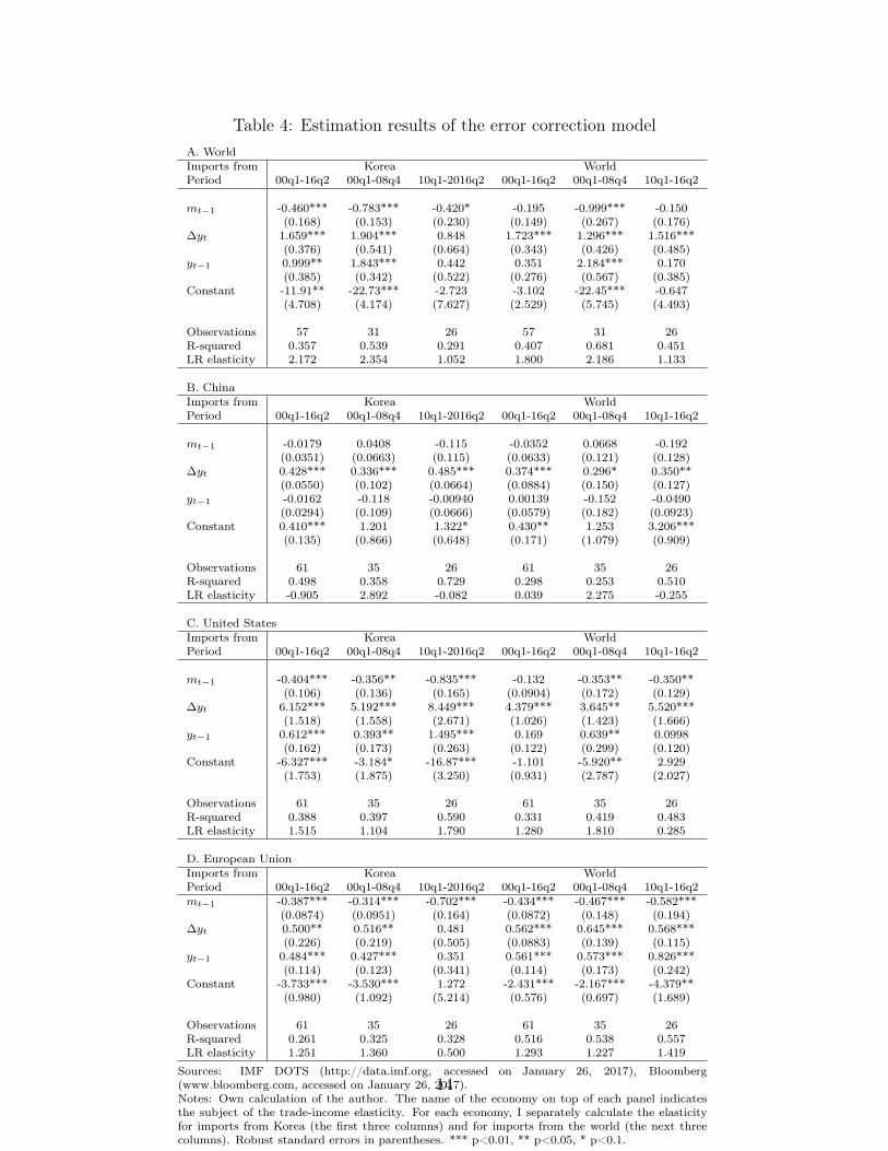
Table 4: Estimation results of the error correction modelA. WorldImports from Korea WorldPeriod 00q1-16q2 00q1-08q4 10q1-2016q2 00q1-16q2 00q1-08q4 10q1-16q2
mt−1 -0.460*** -0.783*** -0.420* -0.195 -0.999*** -0.150(0.168) (0.153) (0.230) (0.149) (0.267) (0.176)
∆yt 1.659*** 1.904*** 0.848 1.723*** 1.296*** 1.516***(0.376) (0.541) (0.664) (0.343) (0.426) (0.485)
yt−1 0.999** 1.843*** 0.442 0.351 2.184*** 0.170(0.385) (0.342) (0.522) (0.276) (0.567) (0.385)
Constant -11.91** -22.73*** -2.723 -3.102 -22.45*** -0.647(4.708) (4.174) (7.627) (2.529) (5.745) (4.493)
Observations 57 31 26 57 31 26R-squared 0.357 0.539 0.291 0.407 0.681 0.451LR elasticity 2.172 2.354 1.052 1.800 2.186 1.133
B. ChinaImports from Korea WorldPeriod 00q1-16q2 00q1-08q4 10q1-2016q2 00q1-16q2 00q1-08q4 10q1-16q2
mt−1 -0.0179 0.0408 -0.115 -0.0352 0.0668 -0.192(0.0351) (0.0663) (0.115) (0.0633) (0.121) (0.128)
∆yt 0.428*** 0.336*** 0.485*** 0.374*** 0.296* 0.350**(0.0550) (0.102) (0.0664) (0.0884) (0.150) (0.127)
yt−1 -0.0162 -0.118 -0.00940 0.00139 -0.152 -0.0490(0.0294) (0.109) (0.0666) (0.0579) (0.182) (0.0923)
Constant 0.410*** 1.201 1.322* 0.430** 1.253 3.206***(0.135) (0.866) (0.648) (0.171) (1.079) (0.909)
Observations 61 35 26 61 35 26R-squared 0.498 0.358 0.729 0.298 0.253 0.510LR elasticity -0.905 2.892 -0.082 0.039 2.275 -0.255
C. United StatesImports from Korea WorldPeriod 00q1-16q2 00q1-08q4 10q1-2016q2 00q1-16q2 00q1-08q4 10q1-16q2
mt−1 -0.404*** -0.356** -0.835*** -0.132 -0.353** -0.350**(0.106) (0.136) (0.165) (0.0904) (0.172) (0.129)
∆yt 6.152*** 5.192*** 8.449*** 4.379*** 3.645** 5.520***(1.518) (1.558) (2.671) (1.026) (1.423) (1.666)
yt−1 0.612*** 0.393** 1.495*** 0.169 0.639** 0.0998(0.162) (0.173) (0.263) (0.122) (0.299) (0.120)
Constant -6.327*** -3.184* -16.87*** -1.101 -5.920** 2.929(1.753) (1.875) (3.250) (0.931) (2.787) (2.027)
Observations 61 35 26 61 35 26R-squared 0.388 0.397 0.590 0.331 0.419 0.483LR elasticity 1.515 1.104 1.790 1.280 1.810 0.285
D. European UnionImports from Korea WorldPeriod 00q1-16q2 00q1-08q4 10q1-2016q2 00q1-16q2 00q1-08q4 10q1-16q2mt−1 -0.387*** -0.314*** -0.702*** -0.434*** -0.467*** -0.582***
(0.0874) (0.0951) (0.164) (0.0872) (0.148) (0.194)∆yt 0.500** 0.516** 0.481 0.562*** 0.645*** 0.568***
(0.226) (0.219) (0.505) (0.0883) (0.139) (0.115)yt−1 0.484*** 0.427*** 0.351 0.561*** 0.573*** 0.826***
(0.114) (0.123) (0.341) (0.114) (0.173) (0.242)Constant -3.733*** -3.530*** 1.272 -2.431*** -2.167*** -4.379**
(0.980) (1.092) (5.214) (0.576) (0.697) (1.689)
Observations 61 35 26 61 35 26R-squared 0.261 0.325 0.328 0.516 0.538 0.557LR elasticity 1.251 1.360 0.500 1.293 1.227 1.419
Sources: IMF DOTS (http://data.imf.org, accessed on January 26, 2017), Bloomberg(www.bloomberg.com, accessed on January 26, 2017).Notes: Own calculation of the author. The name of the economy on top of each panel indicatesthe subject of the trade-income elasticity. For each economy, I separately calculate the elasticityfor imports from Korea (the first three columns) and for imports from the world (the next threecolumns). Robust standard errors in parentheses. *** p<0.01, ** p<0.05, * p<0.1.
14
2.354. But in the third column of Panel A, beta coefficients are mostly insignificant and
the elasticity went down to 1.052. Thus, the relationship between trade and income became
weaker in two aspects: the coefficients became insignificant unlike before, and the level of
trade-income elasticity fell down. I observe the same pattern in the next three columns.
The long-run trade-income elasticity of the world for imports from the world fell from 2.186
before crisis to 1.133 after crisis. The coefficients became mostly insignificant after the crisis
except for β2. Thus, the results of the trade-income elasticity of the world show that the
increase of income creates lower trade after the global financial crisis than before the crisis,
and the relationship itself between trade and income became weaker.
The results slightly vary at the country level. In Panel B, where I present the results
for China, the long-run trade-income elasticity for imports from Korea (to China) fell from
2.892 to -0.082 after the crisis. The elasticity for imports from the world (to China) also
fell from 2.275 to -0.255. China’s decreasing pattern of elasticity is the same as the case
of the world, implying that China played an important role in shaping the pattern of the
decreasing trade-income elasticity. In Panel B, however, both β1 and β3, which are used to
calculate the long-run elasticity, are insignificant in all six columns. This implies that, in
the case of China, the relationship between the current imports growth and the lagged GDP
or lagged imports varies a lot. Thus, the long-run elasticity of China is calculated based on
statistically insignificant coefficients, but China’s decreasing pattern of elasticity is similar
to the world’s.
In Panel C, where I present the results for the US, the long-run trade-income elasticity for
imports from Korea (to US) has increased (from 1.104 to 1.79), and all beta coefficients are
statistically significant both before and after the crisis. The stronger relationship between
US income and its imports from Korea is impressive since the elasticity for imports from
the world went down from 1.810 to 0.825 and β3 is insignificant in the sixth column. The
long-run elasticity of the US for Korean imports may have increased due to the Korea-US
(KORUS) FTA, which came into effect in 2012.
15
In the last panel, I present the results for the EU. The trade-income elasticity for imports
from Korea (to the EU) has the same pattern as the case of the world: β2 and β3 are significant
before crisis but insignificant after crisis, and the elasticity went down from 1.360 to 0.5. The
elasticity for imports from the world (to the EU), however, slightly went up after the crisis,
from 1.227 to 1.419. Also, all coefficients are significant both before and after the crisis.
To sum up, the relationship between the world’s income and the world’s import from both
the world and Korea became weaker after the financial crisis. Such a trend is consistent with
that of China, which confirms the “China factor” in the slowdown literature (Hoekman,
2015). The long-run trade-income elasticity went down in all cases except for the elasticity
of the US for the imports from Korea and the elasticity of the EU for the imports from the
world. Further investigation regarding why there are such exceptions is out of the scope of
this paper but could be a future research topic.
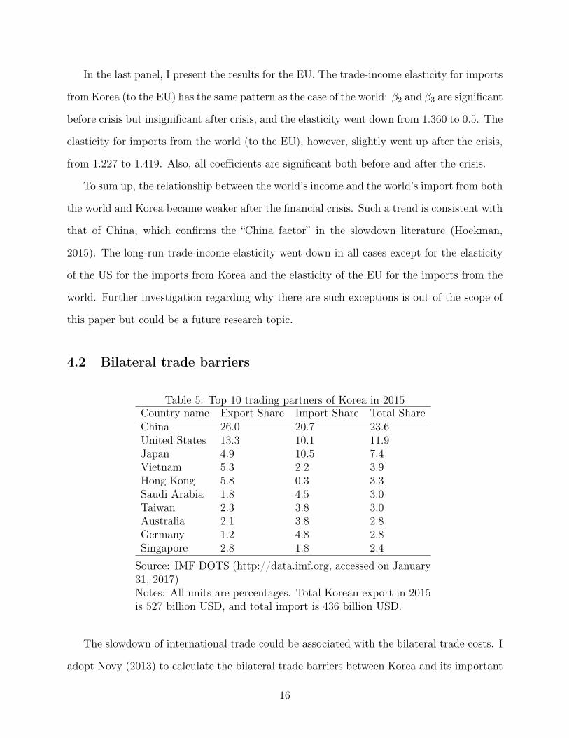
4.2 Bilateral trade barriers
Table 5: Top 10 trading partners of Korea in 2015Country name Export Share Import Share Total ShareChina 26.0 20.7 23.6United States 13.3 10.1 11.9Japan 4.9 10.5 7.4Vietnam 5.3 2.2 3.9Hong Kong 5.8 0.3 3.3Saudi Arabia 1.8 4.5 3.0Taiwan 2.3 3.8 3.0Australia 2.1 3.8 2.8Germany 1.2 4.8 2.8Singapore 2.8 1.8 2.4
Source: IMF DOTS (http://data.imf.org, accessed on January31, 2017)Notes: All units are percentages. Total Korean export in 2015is 527 billion USD, and total import is 436 billion USD.
The slowdown of international trade could be associated with the bilateral trade costs. I
adopt Novy (2013) to calculate the bilateral trade barriers between Korea and its important
16

trade partners, which are listed in Table 5. Novy (2013) derives an analytical way from
the gravity equation to measure bilateral trade barriers. The trade barriers conceptually
measure the costs of international trade compared to domestic trade. The main benefit of
the approach is that it allows one to calculate bilateral trade barriers using directly observable
statistics, such as GDPs and bilateral trade. Specifically, the tariff equivalent trade barrier
between country i and country j is derived as the following:
τij ≡ ((tijtji)/(tiitjj))1/2 − 1 = ((xiixjj)/(xijxji))
1/(2(σ−1)) − 1, (3)
where tij is trade cost that country i faces when exporting to country j, and xij is country
i’s export to country j. tii is country i’s domestic trade costs. Similarly, xii captures country
i’s domestic sales of its total production, which is defined as xii ≡ yi −∑
j xij where yi is
the aggregate goods production of country i. The parameter σ is elasticity of substitution.
Calculation of the trade barriers requires international and domestic trade statistics.
While bilateral trade statistics are readily available from the IMF Direction of Trade Statis-
tics (DOTS), domestic trade statistics need to be constructed. Domestic trade refers to
goods that a country exports to itself (or goods that a country imports from itself), as xii
is defined. The crucial part of measuring xii is to construct the aggregate goods production
yi. Since bilateral trade statistics are gross shipments, which include intermediate goods,
the aggregate goods production needs to be in terms of gross output. The OECD Structural
Analysis (STAN) database offers the statistics but its time coverage is limited to 2011. So
I take the three-step approach of Wei (1996) to construct the aggregate production.9 The
first step is to collect the goods part of quarterly nominal GDP, which generally includes
agriculture, mining, and manufacturing. I obtain the statistics from each trading partner
country’s statistics bureau.10 The second step is to compute the ratio between shipment and
9UN ESCAP and World Bank jointly constructed the annual International Trade Costs database usingthe approach of Novy (2013), but the time coverage is still limited to 2013 as of now. Since I focus on therecent trade slowdown and the collapse of trade, I calculate the trade costs until 2016.
10See appendix for detailed information about the coverage of the goods part of GDP and data source foreach country.
17

value-added using the OECD STAN database. The third step is to calculate the aggregate
goods production as
(Aggregate goods production) =(shipment)
(value added)× (goods part GDP).
The value of elasticity of substitution, σ, is known to range between 5-10 in the literature.
I set σ = 8, but the overall trends are robust to different numbers within the range.
Table 6: Change in bilateral trade barriers between 2012 and 2016Country 2012 2016 Difference Country 2012 2016 DifferenceChina 0.56 0.58 0.02 Saudi Arabia 0.66 0.76 0.10United States 0.79 0.80 0.01 Taiwan 0.36 0.58 0.22Japan 0.70 0.80 0.10 Australia 0.66 0.76 0.11Vietnam 0.69 0.59 -0.09 Germany 0.63 0.65 0.03Hong Kong 0.42 0.53 0.11 Singapore 0.32 0.58 0.26
Source: The calculated trade barriers in Figure 3.Note: The unit of trade barriers is tariff equivalence.
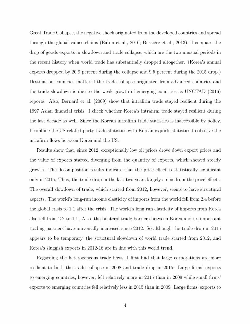
Figure 3 shows the recent trends of bilateral trade costs between Korea and its trading
partners. The vertical axis indicates the level of bilateral trade barriers in terms of tariff
equivalence. Since the value of trade barriers is sensitive to the assigned value of elasticity
of substitution, it is more appropriate to interpret the tariff equivalent values as a relative
measure. The main finding in the results in Figure 3 is that the bilateral trade barriers are
increasing in most of the top trade partner countries since the beginning of the global trade
slowdown around 2011. As Table 6 shows, the increasing trend of bilateral trade barriers is
common to most trade partner countries. Trade barriers with large countries tend to increase
to a smaller extent: the tariff equivalent trade barrier increases 2 percentage points for China,
1 percentage point for United States, and 3 percentage points for Germany between 2012 and
2016. On the contrary, the barriers with middle or smaller countries tend to increase over
10 percentage points. The decrease of trade barriers with Vietnam is exceptional. Over the
periods of the Great Recession and global trade slowdown, the trade barriers with Vietnam
have consistently decreased from 2000. This is related to the exceptional growth of and the
18
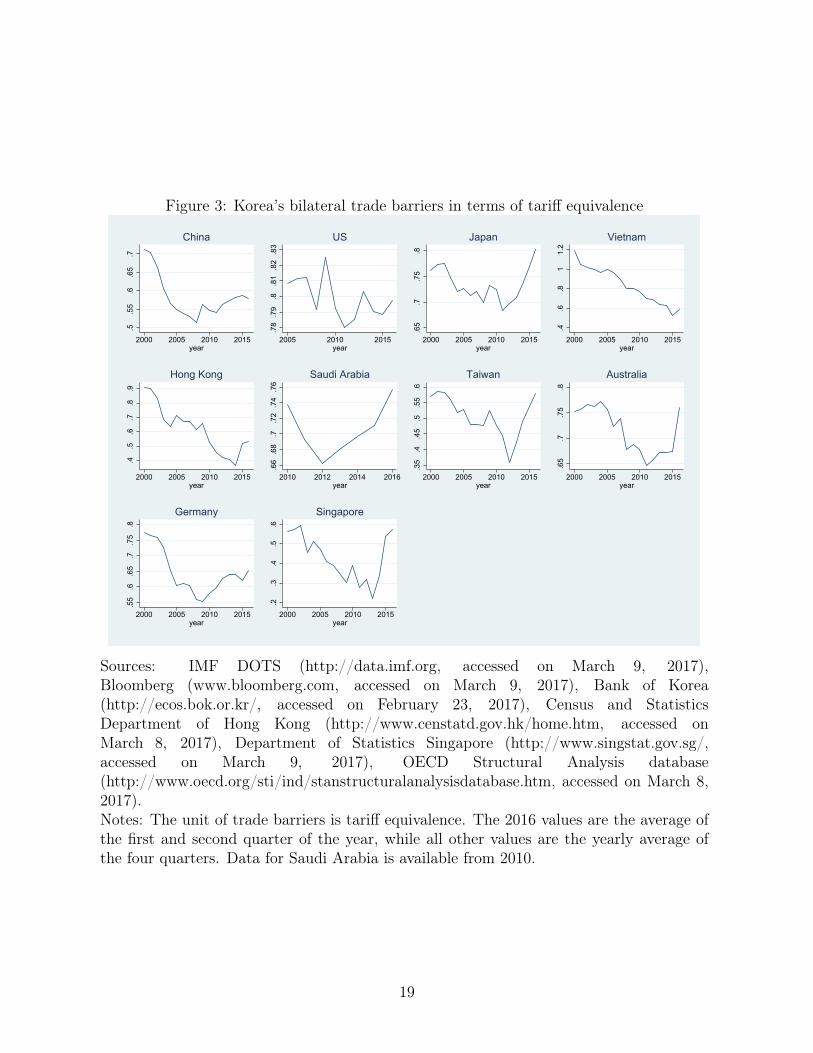
Figure 3: Korea’s bilateral trade barriers in terms of tariff equivalence
.5.5
5.6
.65
.7
2000 2005 2010 2015year
China
.78
.79
.8.8
1.8
2.8
3
2005 2010 2015year
US
.65
.7.7
5.8
2000 2005 2010 2015year
Japan
.4.6
.81
1.2
2000 2005 2010 2015year
Vietnam
.4.5
.6.7
.8.9
2000 2005 2010 2015year
Hong Kong
.66
.68
.7.7
2.7
4.7
6
2010 2012 2014 2016year
Saudi Arabia
.35
.4.4
5.5
.55
.6
2000 2005 2010 2015year
Taiwan
.65
.7.7
5.8
2000 2005 2010 2015year
Australia
.55
.6.6
5.7
.75
.8
2000 2005 2010 2015year
Germany
.2.3
.4.5
.6
2000 2005 2010 2015year
Singapore
Sources: IMF DOTS (http://data.imf.org, accessed on March 9, 2017),Bloomberg (www.bloomberg.com, accessed on March 9, 2017), Bank of Korea(http://ecos.bok.or.kr/, accessed on February 23, 2017), Census and StatisticsDepartment of Hong Kong (http://www.censtatd.gov.hk/home.htm, accessed onMarch 8, 2017), Department of Statistics Singapore (http://www.singstat.gov.sg/,accessed on March 9, 2017), OECD Structural Analysis database(http://www.oecd.org/sti/ind/stanstructuralanalysisdatabase.htm, accessed on March 8,2017).Notes: The unit of trade barriers is tariff equivalence. The 2016 values are the average ofthe first and second quarter of the year, while all other values are the yearly average ofthe four quarters. Data for Saudi Arabia is available from 2010.
19

trade with Vietnam over the past decade.
From the results, it is clear that the bilateral trade barriers that Korea faces have in-
creased during the period of the global trade slowdown. It is worth noting that the trade
barriers show an overall trend of increasing, except for Vietnam. The trend shows that the
cost of international trade is increasing relative to the cost of domestic transactions. While
Korea’s international trade plateaued between 2012 and 2014, the trade barriers were in-
creasing. In this context, the steady decrease of the trade barrier with Vietnam emphasizes
the importance of the relationship between Korea and Vietnam.
There is a caveat when interpreting the trade barrier results. The Novy (2013) method
considers all trade flows that are unexplained by the gravity equation as trade barriers,
which is similar to the concept of the Solow residuals. Thus, the trade barriers could be
overestimated if the global value chains have shrunken after 2011, which is the last year that
the OECD STAN offers the actual ratio of shipment and value added. Unfortunately, the
actual information of the gross shipments after 2012 is unavailable as of now. But when I
use GDP instead of gross shipments to estimate the trade barriers, the increasing pattern
is consistent with the current results. Therefore, while trade barriers seem to be increasing
after around 2012, the magnitude could be adjusted when actual gross-shipment statistics
are available.
5 Heterogeneous aspects of the slowdown
5.1 Destination countries and firm sizes
In this section I ask whether the trade slowdown is concentrated on the trade with emerg-
ing countries. UNCTAD (2016) claims that the trade slowdown is more severe in emerging
countries while the Great Trade Collapse in 2008-09 started from the developed countries
and spread to the rest of the world through the global value chains. I test whether trade
between Korea and emerging countries fell more than trade between Korea and developed
20

countries. I compare the trade growth rate in the trade drop in 2015 and in the midst of the
trade collapse in 2009. While the aggregate trade dropped more severely during the financial
crisis than during the trade slowdown, the effect of destination country could be different in
the two periods because of the different origins of the shocks.
I employ the difference-in-differences method in line with Ariu (2016) to test whether the
effect of destination countries on export growth is different in 2009 and 2015 as below:
∆vjidt = α + β′0Tt + β′1Wdt + β′2Wdt × Tt + δi + εjidt (4)
where ∆vjidt ≡ logvjid,t+1 − logvjid,t denotes the growth of export volume of product j in
industry i from Korea to destination country d between year t and t − 1. To address a
possible seasonality problem, I only use the first half year’s exports in each year in the
dataset. Thus, the dependent variable is the growth rate of exports between the first half of
year t− 1 and the first half of year t. Note that vjidt denotes exports of the first half of year
t, and v′jidt denotes exports of the full year t. The time dimension comprises two periods:
t ∈ {2009, 2015}, which are the periods of trade collapse and trade drop. Tt is a dummy
variable, which is 1 if the period is 2015 and 0 if the period is 2009. Wdt is a vector of two
variables that contain country-level characteristics: one is a destination dummy variable,
which is 1 if the destination d is an emerging country and 0 otherwise. Another variable in
the vector Wdt is the income (GDP) growth rate of the destination country. δi is an industry
fixed effect and εjidt is an error term.
The TRASS dataset tells me the total volume of exports of product j to destination
country d by the size of firms, small, medium, and large. For example, Korea exported 1.31
million USD worth of HS 6-digit product 820570 (vices, clamps & the like) to China in the
first half of 2008. Of 1.31 million USD, large firms sold 1.26 million USD, medium firms sold
0.4 million USD, and small firms sold 0.01 million USD. I omit the firm dimension in the
subscripts of the dependent variable in equation (4) for brevity, but I report results for each
21

group of firms. The industry classification for the industry dummy variable is from TRASS,
which contains 69 industries. The statistics of yearly growth rate of GDP of destination
countries are from the IMF World Economic Outlook.
Table 7: Descriptive statistics of the dataset for the estimation of equation (4)Variable Firm Size Obs Mean Std. Dev. Min Max∆vjidt All 255,916 -0.122 3.050 -17.624 18.532
Large 53,498 -0.3149 3.350 -17.624 18.532Medium 53,512 -0.60 3.181 -15.774 14.831Small 142,406 0.226 2.766 -17.006 16.297
v′jidt All 255,916 1,646,328 3.60e+07 1 7.58e+09Large 53,498 4,995,152 7.61e+07 1 7.58e+09Medium 53,512 1,336,513 1.85e+07 1 2.77e+09Small 142,406 574,129 4,221,590 1 4.46e+08
Tdt All 255,916 0.582 0.49 0 1GDP growth All 255,916 1.57 4.44 -28.1 26.28
Sources: Export statistics from the Korea Customs through Trade Statis-tics Service (accessed on January 19, 2017), IMF World Economic Out-look (https://www.imf.org/external/pubs/ft/weo/2016/02/weodata/index.aspx,accessed on February 16, 2017).Notes: ∆vjidt is the growth of export volume of product j in industry i to destina-tion country d between periods t and t− 1; v′jidt is the unit of yearly exports to acountry-product pair in year t, whose unit is USD. Tdt is 1 if the period is 2015 and0 if the period is 2009. The GDP growth is year-on-year growth rate in percentage.
Table 7 reports descriptive statistics. The dataset contains 255,916 observations, of which
21 percent are large firms, 21 percent are medium firms, and 56 percent are small firms.11
The large firms’ average growth rate is the lowest and their standard deviation of growth rate
is the highest among the three groups of firms. More than half of the number of country-
product pairs, or the extensive margin, belongs to small firms. They export a larger number
of products to more countries than large and medium firms. Small firms export 890 more
intermediate varieties and 378 more consumption varieties than large firms. But large firms
export 5 million USD to a country-product pair on average, which is 8.7 times larger than
the small firms’ average exports to a country-product pair. Although the share of large firms’
exports is falling in Korea, it is still 62.3% in 2016.
11Firm size information was unavailable for the remaining 2 percent.
22

Table 8: Number of exporting countries and productsA. Number of Products
Product type Firm sizeAll Large Medium Small
All 4386 2884 3288 4286Intermediate 2683 1727 2015 2617Capital 601 467 473 592Conumption 1068 668 776 1046Not classified 34 22 24 31
B. Number of Countries
Country type Firm sizeAll Large Medium Small
All 187 178 181 185Emerging 148 140 143 146Advanced 39 38 38 39
Sources: Export statistics from the Korea Cus-toms through Trade Statistics Service (accessedon January 19, 2017), Broad Economic Cate-gories from United Nations Statistics Division(https://unstats.un.org/unsd/cr/registry/regot.asp?Lg=1,accessed on February 3, 2017).Notes: The product type is classified using Basic EconomicCategories, and the country type is classified following IMF.
23
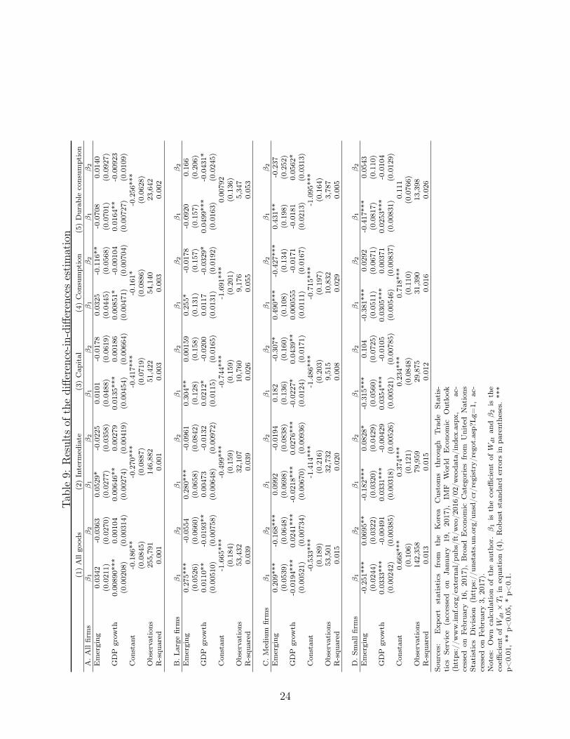
Table9:
Results
ofthediffe
rence-in-differencesestimation
(1)Allgo
ods
(2)Interm
ediate
(3)Cap
ital
(4)Con
sumption
(5)Durab
leconsum
ption
A.Allfirms
β1
β2
β1
β2
β1
β2
β1
β2
β1
β2
Emerging
0.0342
-0.0363
0.0529*
-0.0225
0.0101
-0.017
80.0325
-0.116**
-0.0708
0.0140
(0.0211)
(0.0270)
(0.0277)
(0.0358)
(0.0488)
(0.0619)
(0.0445)
(0.0568)
(0.0701)
(0.0927)
GDP
grow
th0.00890***
0.00104
0.00646**
0.00279
0.0135***
0.00186
0.00851*
-0.00104
0.0164**
-0.00923
(0.00208)
(0.00314)
(0.00274)
(0.00419)
(0.00454)
(0.00664)
(0.00471)
(0.00704)
(0.00727)
(0.0109)
Con
stan
t-0.186**
-0.270***
-0.417***
-0.161*
-0.256***
(0.0845)
(0.0887)
(0.0719)
(0.0886)
(0.0628)
Observation
s255,791
146,882
51,422
54,140
23,642
R-squ
ared
0.001
0.001
0.003
0.003
0.002
B.Large
firms
β1
β2
β1
β2
β1
β2
β1
β2
β1
β2
Emerging
0.275***
-0.0554
0.280***
-0.0961
0.304**
0.00159
0.255*
-0.0178
-0.0920
0.166
(0.0526)
(0.0660)
(0.0658)
(0.0842)
(0.128)
(0.158)
(0.131)
(0.157)
(0.157)
(0.206)
GDP
grow
th0.0110**
-0.0193**
0.00473
-0.0132
0.0212*
-0.0200
0.0117
-0.0329*
0.0499***
-0.0431*
(0.00510)
(0.00758)
(0.00648)
(0.00972)
(0.0115)
(0.0165)
(0.0131)
(0.0192)
(0.0163)
(0.0245)
Con
stan
t-1.665***
-0.499***
-0.744***
-1.691***
0.00792
(0.184)
(0.159)
(0.159)
(0.201)
(0.136)
Observation
s53,432
32,107
10,760
9,176
5,347
R-squ
ared
0.039
0.039
0.026
0.055
0.053
C.Medium
firms
β1
β2
β1
β2
β1
β2
β1
β2
β1
β2
Emerging
0.209***
-0.168***
0.0992
-0.0194
0.182
-0.307*
0.49
0***
-0.427***
0.431**
-0.237
(0.0539)
(0.0648)
(0.0698)
(0.0838)
(0.136)
(0.160)
(0.108)
(0.134)
(0.198)
(0.252)
GDP
grow
th-0.0194***
0.0241***
-0.0218***
0.0276***
-0.0227*
0.0439**
0.000555
-0.0171
-0.0181
0.0562*
(0.00521)
(0.00734)
(0.00670)
(0.00936)
(0.0124)
(0.0171)
(0.0111)
(0.0167)
(0.0213)
(0.0313)
Con
stan
t-0.533***
-1.414***
-1.486***
-0.715***
-1.095**
*(0.189)
(0.216)
(0.203)
(0.197)
(0.164)
Observation
s53,501
32,732
9,515
10,832
3,787
R-squ
ared
0.015
0.020
0.008
0.029
0.005
D.Sm
allfirms
β1
β2
β1
β2
β1
β2
β1
β2
β1
β2
Emerging
-0.251***
0.0695**
-0.182***
0.0828*
-0.315***
0.104
-0.381***
0.0292
-0.417**
*0.0543
(0.0244)
(0.0322)
(0.0320)
(0.0429)
(0.0560)
(0.0725)
(0.0511)
(0.0671)
(0.0817)
(0.110)
GDP
grow
th0.0333***
-0.00491
0.0331***
-0.004
290.0354***
-0.0105
0.0305***
0.00371
0.0253
***
-0.0104
(0.00242)
(0.00385)
(0.00318)
(0.00526)
(0.00521)
(0.00785)
(0.00546)
(0.00837)
(0.00831)
(0.0129)
Con
stan
t0.668***
0.374***
0.234***
0.718***
0.111
(0.106)
(0.121)
(0.0848)
(0.110)
(0.0766)
Observation
s142,358
79,959
29,875
31,390
13,398
R-squ
ared
0.013
0.015
0.012
0.016
0.026
Sources:
Exp
ort
statistics
from
the
Korea
Customs
throug
hTrade
Statis-
tics
Service
(accessed
onJa
nuary
19,2017),
IMF
World
Econo
mic
Outlook
(https://w
ww.im
f.org/externa
l/pu
bs/ft/weo/2016/02/w
eoda
ta/ind
ex.aspx,
ac-
cessed
onFe
brua
ry16,2017),
Broad
Econo
mic
Categoriesfrom
United
Nations
Statistics
Division
(https://u
nstats.un.org/un
sd/cr/registry/regot.asp?L
g=1,
ac-
cessed
onFe
brua
ry3,
2017).
Notes:Owncalculationof
theau
thor.β1is
thecoeffi
cientofW
dtan
dβ2is
the
coeffi
cientofW
dt×Ttin
equa
tion
(4).
Rob
uststan
dard
errors
inpa
rentheses.
***
p<0.01,**
p<0.05,*p<
0.1.
24
A positive and significant β1 for the emerging country variable will show that export
growth to emerging countries was higher than that to advanced countries in 2009, after
controlling for the changes in exports due to GDP growth. Such a result will be consistent
with the claim that the Great Trade Collapse was more severe among developed countries.
It is important to note that I control for the GDP growth rate in the regression. Thus, I
measure the effect of the destination countries in 2015 compared to 2009, which is a “pure
country” effect. Intermediate goods export is about 2/3 of all Korean exports to emerging
countries, and 1/3 of all Korean exports to advanced countries. Thus, the “pure country”
effect considers the composition of goods rather than income growth effect.
A negative and significant β2 for the emerging country variable will show that Korean
export growth to emerging countries has weakened in 2015 compared to 2009, which is con-
sistent with the claim that weakening emerging economies partly caused the trade slowdown.
If the sum of β1 and β2 is positive, then the average export growth to emerging countries
was higher than that to advanced countries in 2015.
I present the results of the estimation in equation (4) in Table 9. β1’s are positive
and significant for all goods in the case of large firms and medium firms, but negative and
significant in the case of small firms. The change in export growth rate to emerging countries
during the 2008-09 trade collapse was 27.5 percent higher than advanced countries for large
firms and 20.9 percent higher for medium firms. Thus Korean exports to emerging countries
by large and medium firms did stay resilient in 2009 compared to exports to advanced
countries. But the change in export growth rate during 2008-09 to emerging countries was
25.1 percent lower for small firms. Such severe drop of exports to emerging countries by
small firms is prevalent in all goods categories: -18.2 percent for intermediate goods, -31.5
percent for capital goods, -38.1 percent for consumption goods, and -41.7 percent for durable
consumption goods.
As expected, the signs reverse for β2’s. They are negative but largely insignificant for
large firms. Overall, the large firms’ export growth to emerging countries is 5.5 percent
25

lower than export growth to advanced countries in 2015 compared to 2009, but the effect
is statistically insignificant. The β2 coefficients are negative and significant at 1 percent for
medium firms for all goods, and the consumption goods drive the result. Overall, the export
growth of medium firm exports to emerging countries dropped by 16.8 percent for all goods,
and by 42.7 percent for consumption goods in 2015 compared to 2009. The results imply
that the 2015 trade drop was due to weak demand in the emerging countries suffering from
the low oil prices. Stronger drop in consumption goods exports to these countries is evidence
of this. Then why did medium firms suffer more severely than large firms during the trade
slowdown? One possibility is that while the trade collapse was shockingly sudden, the 2015
trade drop occurred after more than two years of trade slowdown. And larger firms were
able to stay more stable than medium firms thanks to their uncertainty managements.
The β2 coefficients for small firms are positive and significant, indicating that the small
firms’ export growth to emerging countries is 7.0 percent higher in the 2015 trade drop than
in the 2009 trade collapse. The coefficient for the intermediate goods sector is the most
significant. But a caveat here is that the exports by small firms most severely dropped
among all groups of firms in 2009. As explained above, the sum of β1 and β2 is the effect
of emerging countries on Korea’s exports in 2015, and it is still the lowest for small firms,
-0.18, where the sum is 0.22 for large firms and 0.04 for medium firms. Thus, exports of
small firms to emerging countries were impacted the most during the trade drop in 2015,
but they did better compared to when financial crisis hit. The export of large and medium
firms to emerging countries suffered more in 2015 compared to the trade collapse.
It is interesting that, after controlling for the GDP growth rates, the export drop in 2015
to emerging countries was more severe among large and medium firms than that of small
firms. Such differing patterns between large and medium firms versus small firms hold in
all goods categories, intermediate, capital, consumption, and durable consumption products,
except for the capital goods categories of medium firms. Investigating the reason behind the
relatively sound performances of small firms will be a meaningful future research topic.
26

5.2 Intrafirm trade
Bernard et al. (2009) report that international transactions between related parties, or
intrafirm trade, stayed largely intact during the Asian financial crisis in 1997, and Altomonte
et al. (2011) show that intrafirm trade dropped and recovered faster than arm’s length trade
during the Great Trade Collapse. So I ask whether Korean intrafirm trade is relatively intact
during the trade collapse in 2009 and the recent trade slowdown. Unfortunately, the access
to Korean intrafirm trade statistics is restricted as of now and there is no public source of
the data. But I measure the intrafirm trade between Korea and the US by combining two
available datasets. One is TRASS and the other is the US related-party trade database
from the US Census. The related-trade database offers information on all international
transactions between the US and all of its bilateral trading partners at the 5-digit NAICS
(North American Industrial Classification) level. For each industry and year, the database
reports total transactions, related-party transactions and non-related party transactions for
both export and import. A transaction is classified as related party if one party of the
transaction owns more than 10 percent of the other party in the case of exports and more
than 6 percent in the case of imports. Thus related-party transactions information is often
used as a proxy of intrafirm trade in the international trade literature. From the related-
trade database, I use the information on the share of intrafirm trade between the US and
Korea in each NAICS 5-digit industry i as follows:
(Intrafirm share)it =(total related-party transactions)it
(total transactions)it.
I match the related-party trade database with the Korean exports statistics from TRASS
using the concordance table between NAICS 5-digit and HS 6-digit published from the US
Census Bureau. The sample periods are from 2006 to 2014, since the most recent statistics
are for 2014. The related-party trade database gives the intrafirm trade share information
for each HS 6-digit product. I repeat the decomposition exercise of section 3 for the group
27

Figure 4: Growth rates of related-party exports to the US
-.4-.2
0.2
.4.6
%
2006 2008 2010 2012 2014Year
High related-party Low related-party
Export Growth Rate
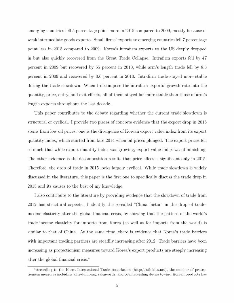
Sources: Export statistics from the Korea Customsthrough Trade Statistics Service (accessed on January 19,2017), (http://sasweb.ssd.census.gov/relatedparty/, accessedon March 27, 2017).Notes: The left axis indicates the year-on-year growth ratesof high and low related-party exports from Korea to the US.High (low) related-party group captures exports by the in-dustries whose share of related-party exports out of total ex-ports is below (above) the first (third) quartile.
of products whose related-party share is above the third quartile, which I call “high related-
party” and another group of products below the first quartile, which I call “low related-party”.
I use the high related-party share group as a proxy for intrafirm exports, and the low related-
party share group as a proxy for arm’s length exports to the US from Korea.
Figure 4 presents the year-on-year export growth rate separately for the high and low
related-party group. Intrafirm trade fluctuated more but recovered faster during the Great
Trade Collapse, and stayed more stable during the slowdown. The response of intrafirm
trade during the GTC is similar to that of French intrafirm trade reported by Altomonte
et al. (2011) in that the intrafirm exports to the US promptly adjust to the macroeconomic
shock. The high related-party exports dropped by 46.8 percent in 2009 and recovered by
55.3 percent in 2010, whereas the low related-party exports dropped by 8.3 percent in 2009
28
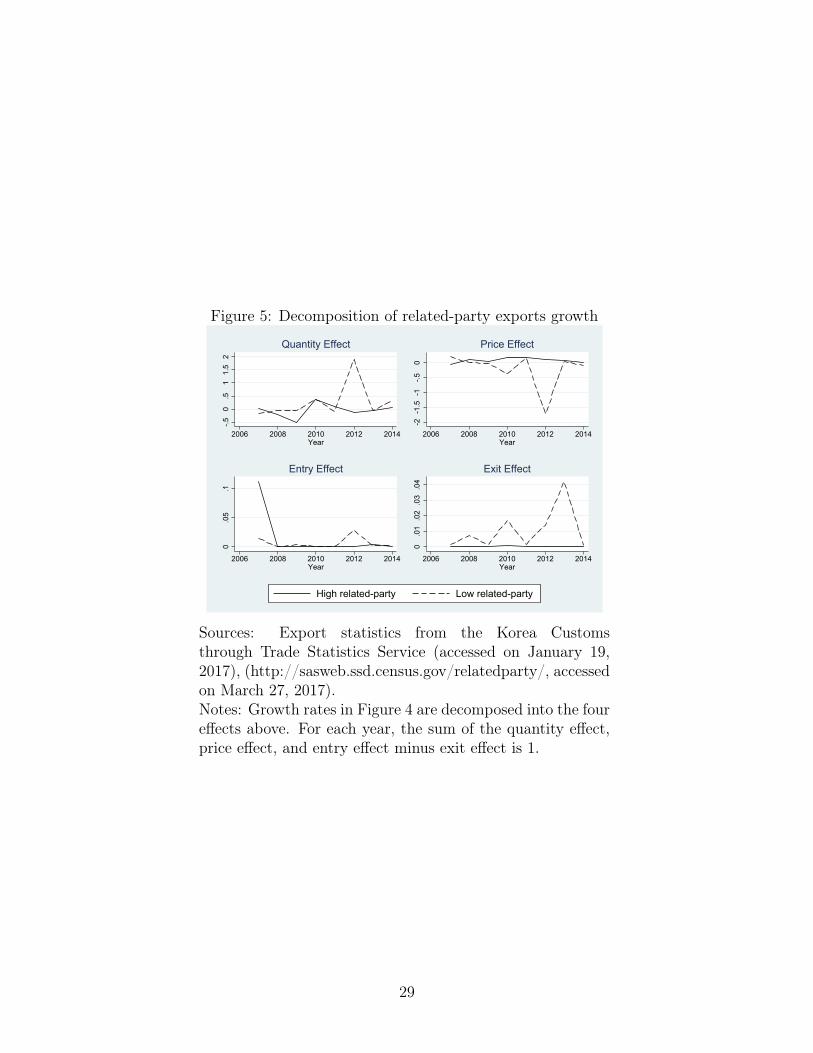
Figure 5: Decomposition of related-party exports growth
-.50
.51
1.5
2
2006 2008 2010 2012 2014Year
Quantity Effect
-2-1
.5-1
-.50
2006 2008 2010 2012 2014Year
Price Effect
0.0
5.1
2006 2008 2010 2012 2014Year
Entry Effect
0.0
1.0
2.0
3.0
4
2006 2008 2010 2012 2014Year
Exit Effect
High related-party Low related-party
Sources: Export statistics from the Korea Customsthrough Trade Statistics Service (accessed on January 19,2017), (http://sasweb.ssd.census.gov/relatedparty/, accessedon March 27, 2017).Notes: Growth rates in Figure 4 are decomposed into the foureffects above. For each year, the sum of the quantity effect,price effect, and entry effect minus exit effect is 1.
29
and recovered by 0.6 percent in 2010. Thus, although the intrafirm trade between Korea and
the US dropped deeper than the arm’s length trade during the GTC, intrafirm trade also
strongly recovered in the subsequent years. The pattern of deeper drop and faster recovery
is found in the aggregate export flows during the GTC, and it could be the case that large
firms, which are the majority of the exports, are involved in the intrafirm trade. Due to
the lack of related party trade data in 2015, I cannot compare the patterns of intrafirm and
arm’s length trade in the 2015 trade drop, but this could be done in the near future when
the data is available.
Figure 5 shows the decomposition of the growth rate into quantity, price, entry, and exit
effects. I do not run OLS regressions for intrafirm trade between Korea and the US because
there is only one observation (country) in each year. The decomposition results show that
the high related-party group stayed stable in price, entry, and exit effects throughout the
years. The quantity effect of high related party exports fell by 49.8 percent in 2009, reflecting
the huge drop of intrafirm exports in 2009. But the price effect of the high related-party
group fell by only 6.7 percent in 2009, showing that the trade drop of 2009 was mostly due
to the quantity effect. The pattern is similar in low related-party trade. In later years, when
trade slowdown has continued, all four effects of the high related-party stay more stable than
the low-related party. In 2012, when the low related-party’s quantity effect jumped and its
price effect dropped, the four effects of the aggregate export from Korea to the US showed
the same patterns. Thus, it seems that, unlike the total export fluctuations in quantity and
price effects, intrafirm trade, at least with the US, stayed more stable and resilient during
the period of slowdown.
6 Conclusion and policy implications
Observing the unusual trade trends of the world and Korea in the last decade, I investigate
detailed features of the trade collapse and slowdown at both aggregate and disaggregated
30
levels. I show that Korea’s recent export drop in 2015 is apparently accompanied with
low oil prices. Thus it seems natural that exports in the near future will show positive
growth if oil prices continue their recovery. There is evidence, however, that points to the
structural changes of exports. The long-run trade-income elasticity has shrunken after the
global financial crisis, and Korea’s bilateral trade barriers with most of its important trading
partners have tightened since 2011.
I also present evidence regarding the heterogeneities in disaggregated trade flows. Over-
all, the exports of large corporations are more resilient than that of medium and small
enterprises during the trade collapse and slowdown, but small firms fared better during the
trade slowdown than the trade collapse. I provide rare evidence regarding Korean intrafirm
exports’ stability during the period of trade slowdown. In the long run, analyzing value-
added exports would be helpful to understand the current slowdown of the international
trade, when the value-added data for the current years are available in the future.12
The results of this paper offer various policy implications. First, to lower the adverse
effect of oil price fluctuations on export growth, it is important to diversify the export
products. Korea’s export prices are strongly affected by oil prices since Korea completely
depends on foreign sources when it comes to its oil supplies. But there is a way to mitigate
the negative effect of oil prices fluctuations. Haddad et al. (2010) point out that, in the
US during the global financial crisis, the prices of homogenous goods plunged but the prices
of differentiated goods stayed stable. The situation was similar in Korea during the trade
slowdown period. According to the Bank of Korea, between 2012-2016, export prices of
chemical, primary metal, and coals and petroleum products fell most while the export prices
of transport equipments and general machineries hardly changed. Thus, diversifying the
export products to include more differentiated products would lower the temporary price
effects due to oil price fluctuations.
Second, considering the fact that the long-run trade-income elasticity of the world has
12Since the export value-added database from the World Bank or the OECD does not cover 2015-16, asof now it is difficult to measure how value-added exports changed during the trade drop periods.
31

shrunken, it is likely that future export growth will be modest unlike before the mid-2000s.
China’s average growth rate in 2002-11 was 10.6, but was 7.4 in 2012-15 according to the IMF.
As China is transforming itself from “the factory of the world” into a domestic-consumption-
centered economy, the international trade through global value chains will likely continue to
be slow. It is important for policy-makers to have a long-run perspective and be ready to
navigate the age of slow trade to maximize the benefits from international trade.
Third, while bilateral trade barriers between Korea and its important trading partners
are universally increasing, the trade barriers of Vietnam have continuously lowered since
2000. The diminishing trend of the trade barriers between Korea and Vietnam has been
intact during the period of the trade collapse and slowdown. It seems, therefore, likely
that the trend will continue in the future, and such trend may apply to the trade barriers
between Korea and other ASEAN countries. Korea has free trade agreements in effect with
both Vietnam and ASEAN, but the utilization rates of the two FTAs are low at 36.0 percent
and 52.3 percent as of 2016. Therefore, it will be beneficial to enhance the utilization rates
through economic cooperations with Vietnam and other ASEAN countries.
Lastly, at a disaggregated level, export flows show heterogenous patterns depending on
firm sizes, product categories, destination countries, and organization mode of exports. The
results in section 5 identify robust export flows during the recent slowdown and drop, on
which policy makers can focus attention and encourage these sectors to become main export
industries in the age of slow trade. The share of exports by small firms has been rising
during the slowdown period according to the Korea International Trade Association, which
is encouraging. Thus, policy makers may further support small firms by helping them to
transform their manufacturing facilities into smart factories to boost productivity and by ef-
fectively operating export finances, which Korean small firms request most as export policies.
Also, as emerging countries are expected to continue their slow growth in the near future,
exports, especially consumption goods, to advanced countries will be promising. Given the
mild price effects in the growth of intrafirm exports, it is worth noting that FDI-induced
32

exports may contribute to the stabilization of export flows.
33
References
Altomonte, C., F. Di Mauro, G. I. P. Ottaviano, A. Rungi, and V. Vicard (2011). Global
value chains during the great trade collapse: a bullwhip effect?
Ariu, A. (2016). Crisis-proof services: Why trade in services did not suffer during the 2008–
2009 collapse. Journal of International Economics 98, 138–149.
Arvis, J.-F., Y. Duval, B. Shepherd, C. Utoktham, and A. Raj (2016). Trade costs in the
developing world: 1996–2010. World Trade Review 15 (03), 451–474.
Baldwin, R. E. (2009). The great trade collapse: Causes, Consequences and Prospects. CEPR.
Bems, R., R. C. Johnson, and K.-M. Yi (2010). Demand spillovers and the collapse of trade
in the global recession. IMF Economic Review 58 (2), 295–326.
Bernard, A. B., J. B. Jensen, S. J. Redding, and P. K. Schott (2009). The margins of us
trade. The American Economic Review 99 (2), 487–493.
Bussière, M., G. Callegari, F. Ghironi, G. Sestieri, and N. Yamano (2013). Estimating trade
elasticities: Demand composition and the trade collapse of 2008-2009. American Economic
Journal: Macroeconomics 5 (3), 118–51.
Constantinescu, C., A. Mattoo, and M. Ruta (2015). The global trade slowdown: Cyclical
or structural? IMF Working Paper .
Eaton, J., M. Eslava, M. Kugler, and J. Tybout (2008). Export dynamics in colombia: Firm-
level evidence. In E. Helpman, D. Marin, and T. Verdier (Eds.), The Organization of Firms
in a Global Economy, Chapter 8, pp. 231–272. Cambridge, MA: Harvard University Press.
Eaton, J., S. Kortum, B. Neiman, and J. Romalis (2016, November). Trade and the global
recession. American Economic Review 106 (11), 3401–38.
34
Escaith, H., N. Lindenberg, and S. Miroudot (2010). International supply chains and trade
elasticity in times of global crisis.
Evenett, S. and J. Fritz (2015). The tide turns? trade, protectionism, and slowing global
growth.
Gopinath, G., O. Itskhoki, and B. Neiman (2012). Trade prices and the global trade collapse
of 2008–09. IMF Economic Review 60 (3), 303–328.
Haddad, M., A. Harrison, and C. Hausman (2010). Decomposing the great trade collapse:
Products, prices, and quantities in the 2008-2009 crisis. Technical report, National Bureau
of Economic Research.
Hoekman, B. (2015). The global trade slowdown: A new normal. VoxEU ed., CEPR.
Levchenko, A. A., L. T. Lewis, and L. L. Tesar (2010). The collapse of international trade
during the 2008–09 crisis: in search of the smoking gun. IMF Economic Review 58 (2),
214–253.
Novy, D. (2013). Gravity redux: measuring international trade costs with panel data. Eco-
nomic inquiry 51 (1), 101–121.
Osnago, A. and S. W. Tan (2016). Disaggregating the impact of the internet on international
trade.
UNCTAD (2016). Key Indicators and Trends in International Trade. United Nations Con-
ference on Trade and Development.
Wei, S.-J. (1996). Intra-national versus international trade: how stubborn are nations in
global integration? Technical report, National Bureau of Economic Research.
Wu, H. X. (2012). Measuring gross output, value added, employment and labor productivity
of the chinese economy at industry level, 1987-2008–an introduction to the cip database
(round 1.0). Technical report, RIETI Discussion Paper Series.
35
Appendix
A List of advanced and emerging countries
1 Advanced countries
Australia, Austria, Belgium, Canada, Cyprus, Czech Republic, Denmark, Estonia, Finland,
France, Germany, Greece, Hong Kong (Special Administrative Region of China), Iceland,
Ireland, Israel, Italy, Japan, Latvia, Lithuania, Luxembourg, Macao (Special Administra-
tive Region of China), Malta, Netherlands, New Zealand, Norway, Portugal, Puerto Rico,
San Marino, Singapore, Slovakia, Slovenia, Spain, Sweden, Switzerland, Taiwan (Republic of
China), United Kingdom, United States Minor Outlying Islands, United States of America
2 Emerging countries
Afghanistan, Albania, Algeria, Angola, Antigua and Barbuda, Argentina, Armenia, Azer-
baijan, Bahamas, Bahrain, Bangladesh, Barbados, Belarus, Belize, Benin, Bhutan, Bolivia,
Bosnia and Herzegovina, Botswana, Brazil, Brunei, Darussalam, Bulgaria, Burkina Faso, Bu-
rundi, Cote d’Ivoire, Cambodia, Cameroon, Central African Republic, Chad, Chile, China,
Colombia, Comoros, Congo (Brazzaville), Democratic Republic of the Congo, Costa Rica,
Croatia, Djibouti, Dominica, Dominican Republic, Ecuador, Egypt, El Salvador, Equato-
rial Guinea, Eritrea, Ethiopia, Fiji, Gabon, Gambia, Georgia, Ghana, Grenada, Guatemala,
Guinea, Guinea-Bissau, Guyana, Haiti, Honduras, Hungary, India, Indonesia, Islamic Re-
public of Iran, Iraq, Jamaica, Jordan, Kazakhstan, Kenya, Kiribati, Kuwait, Kyrgyzstan,
Lao PDR, Lebanon, Lesotho, Liberia, Libya, Republic of Macedonia, Madagascar, Malawi,
Malaysia, Maldives, Mali Marshall Islands, Mauritania, Mauritius, Mexico, Federated States
of Micronesia, Moldova, Mongolia, Montenegro, Morocco, Mozambique, Myanmar, Namibia,
Nepal, Nicaragua, Niger, Nigeria, Oman, Pakistan, Palau, Panama, Papua New Guinea,
Paraguay, Peru, Philippines, Poland, Qatar, Romania, Russian Federation, Rwanda, Saint
Kitts and Nevis, Saint Lucia, Saint Vincent and Grenadines, Samoa, Sao Tome and Principe,
Saudi Arabia, Senegal, Serbia, Seychelles, Sierra Leone, Solomon Islands, South Africa, South
Sudan, Sri Lanka, Sudan, Suriname, Swaziland, Syrian Arab Republic (Syria), Tajikistan,
36
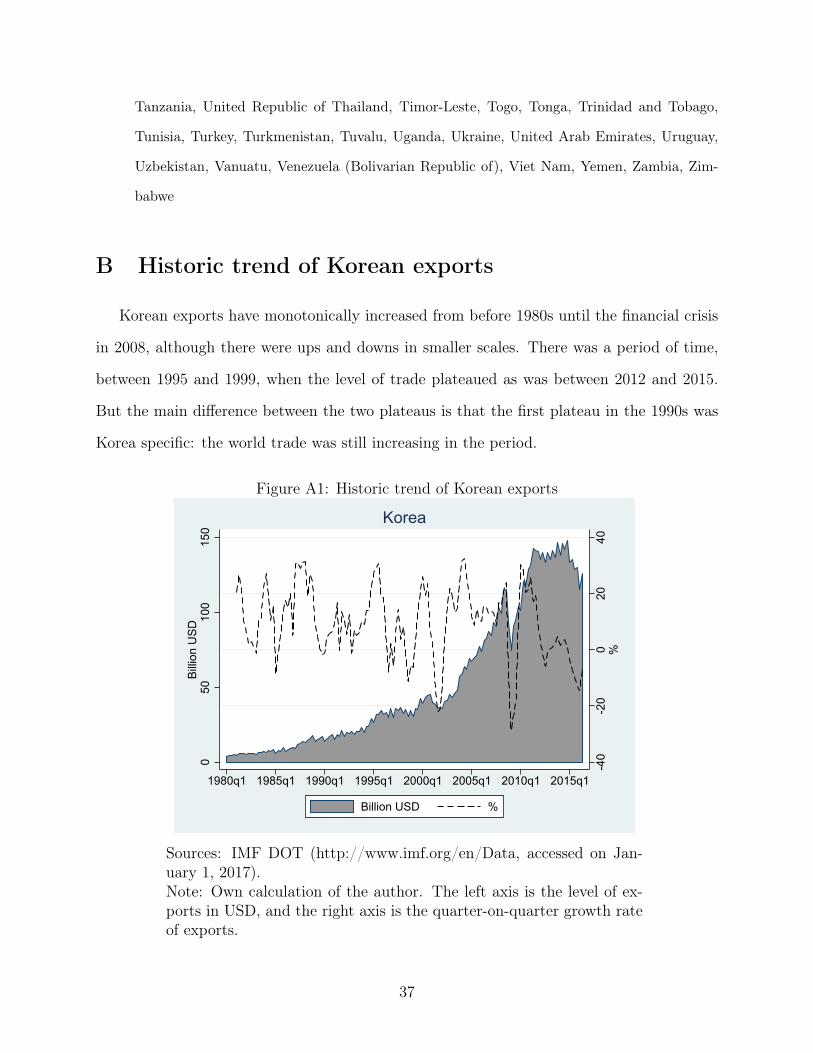
Tanzania, United Republic of Thailand, Timor-Leste, Togo, Tonga, Trinidad and Tobago,
Tunisia, Turkey, Turkmenistan, Tuvalu, Uganda, Ukraine, United Arab Emirates, Uruguay,
Uzbekistan, Vanuatu, Venezuela (Bolivarian Republic of), Viet Nam, Yemen, Zambia, Zim-
babwe
B Historic trend of Korean exports
Korean exports have monotonically increased from before 1980s until the financial crisis
in 2008, although there were ups and downs in smaller scales. There was a period of time,
between 1995 and 1999, when the level of trade plateaued as was between 2012 and 2015.
But the main difference between the two plateaus is that the first plateau in the 1990s was
Korea specific: the world trade was still increasing in the period.
Figure A1: Historic trend of Korean exports
-40
-20
020
40%
050
100
150
Bill
ion
US
D
1980q1 1985q1 1990q1 1995q1 2000q1 2005q1 2010q1 2015q1
Billion USD %
Korea
Sources: IMF DOT (http://www.imf.org/en/Data, accessed on Jan-uary 1, 2017).Note: Own calculation of the author. The left axis is the level of ex-ports in USD, and the right axis is the quarter-on-quarter growth rateof exports.
37
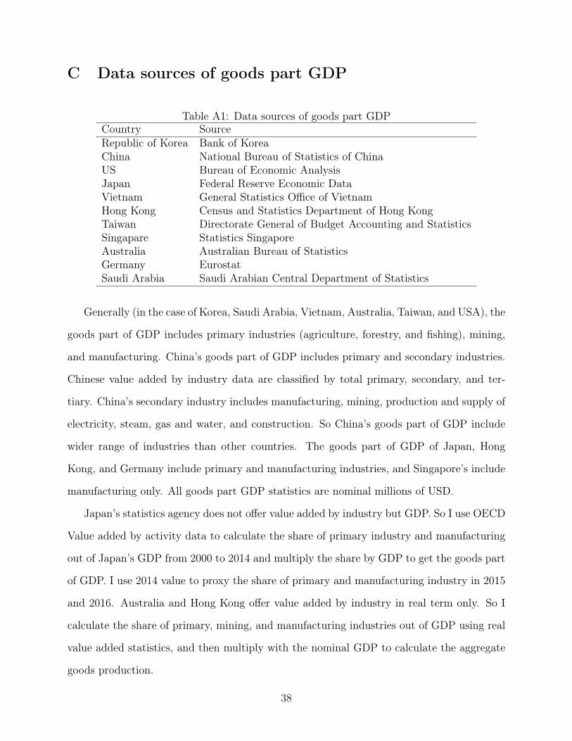
C Data sources of goods part GDP
Table A1: Data sources of goods part GDPCountry SourceRepublic of Korea Bank of KoreaChina National Bureau of Statistics of ChinaUS Bureau of Economic AnalysisJapan Federal Reserve Economic DataVietnam General Statistics Office of VietnamHong Kong Census and Statistics Department of Hong KongTaiwan Directorate General of Budget Accounting and StatisticsSingapare Statistics SingaporeAustralia Australian Bureau of StatisticsGermany EurostatSaudi Arabia Saudi Arabian Central Department of Statistics
Generally (in the case of Korea, Saudi Arabia, Vietnam, Australia, Taiwan, and USA), the
goods part of GDP includes primary industries (agriculture, forestry, and fishing), mining,
and manufacturing. China’s goods part of GDP includes primary and secondary industries.
Chinese value added by industry data are classified by total primary, secondary, and ter-
tiary. China’s secondary industry includes manufacturing, mining, production and supply of
electricity, steam, gas and water, and construction. So China’s goods part of GDP include
wider range of industries than other countries. The goods part of GDP of Japan, Hong
Kong, and Germany include primary and manufacturing industries, and Singapore’s include
manufacturing only. All goods part GDP statistics are nominal millions of USD.
Japan’s statistics agency does not offer value added by industry but GDP. So I use OECD
Value added by activity data to calculate the share of primary industry and manufacturing
out of Japan’s GDP from 2000 to 2014 and multiply the share by GDP to get the goods part
of GDP. I use 2014 value to proxy the share of primary and manufacturing industry in 2015
and 2016. Australia and Hong Kong offer value added by industry in real term only. So I
calculate the share of primary, mining, and manufacturing industries out of GDP using real
value added statistics, and then multiply with the nominal GDP to calculate the aggregate
goods production.
38
Since the goods part GDP statistics are originally in local currency, I convert them to
millions of US dollars using the quarterly average exchange rate from Bank of Korea for
Korea, China, Japan, Singapore, and Vietnam, Bloomberg for Australia, Germany, Hong
Kong, Saudi Arabia, and Central Bank of Republic of China (Taiwan) for Taiwan.
The ratio of gross output and value added for the total economy information is from the
OECD Structural Analysis (STAN) database for USA, Germany, Korea, and Japan between
2000 and 2011. The OECD STAN offers the information about Australia for manufacturing
industry only between 1990 and 1999, which is 3.23 on average. The goods part GDP
includes primary and mining industries as well, and Arvis et al. (2016) report that the gross
output and value added ratio for agriculture ranges between 1.74 and 1.93. So I use the
weighted average of the two industries, which is 2.90, as a proxy for the ratio for Australia.
I use the latest value available as a proxy of the ratio for the recent years. The ratio of
gross output and value added used for China is 2.85, which is an average value of the ratio
between 1987-2008 according to Wu (2012). For Vietnam, Hong Kong, Singapore, Taiwan,
and Saudi Arabia, I use the yearly average of other Asian developing countries, Korea and
China.
39