Analyzing Urban Systems: Have Mega-Cities Become …erossi/WBGlaeser040412.pdf · Analyzing Urban Systems: Have Mega-Cities Become Too Large? Klaus Desmet Universidad Carlos III Esteban

Analyzing Urban Systems:

Have Mega-Cities Become Too Large?∗

Klaus Desmet

Universidad Carlos III

Esteban Rossi-Hansberg

Princeton University

April 4, 2012

Abstract

With the trend toward greater urbanization and the rapid emergence of mega-cities contin-

uing unabated, many policy makers ask themselves whether some cities are becoming too large,

and whether policies should be aimed at stimulating the growth of intermediate-sized cities.

This chapter explains how a simple model of a system of cities, together with some basic urban

and aggregate data, can be used to answer some of the following questions. Would there be

any welfare gains from reducing the size of mega-cities and increasing that of intermediate-sized

cities? Is there any sense in implementing policies that make cities more equal in terms of

efficiency and amenities? Should infrastructure investments be focused on improving life in the

largest cities or in the intermediate cities? The aim is to provide quantitative answers to these

questions by using data from the U.S. and two large developing countries, China and Mexico.

1. INTRODUCTION

The trend toward ever greater urbanization is continuing unabated across the globe. According

to the United Nations, by 2025 close to 5 billion people will live in urbanized areas. Many cities,

especially in the developing world, are set to explode in size. The Nigerian city of Lagos, for example,

is expected to increase its population by 50%, to nearly 16 million, in the next decade and a half (UN-

Habitat 2010). Naturally, there is an active debate on whether restricting the growth of mega-cities

is desirable, and whether it can make residents of those cities and their countries better off.

Importantly, this debate is not so much about urbanization per se –whether people should move

to cities or stay in the countryside– but rather about whether (some) of the world’s mega-cities

are creating mega-problems that could be avoided with suitable policies. People flock to cities in

∗We acknowledge the support of the International Growth Centre at LSE (Grant RA-2009-11-015).

1

search of higher paying jobs and better amenities. Many of the world’s large metropolises, such as

Los Angeles and Mumbai, are highly productive and are located next to large bodies of water. As

cities grow in size, however, they start suffering from increased congestion, higher crime rates, and

air pollution. How fast the benefits of efficiency and amenities erode with population size because

of increasing congestion costs depends on the quality of governance, responsible for the provision

of road infrastructure, sewage systems, clean water, and security. Cities obviously differ in their

efficiency, their amenities and the quality of their governance, and there is no one answer to what

their optimal size should be. We need analytical tools that can help us evaluate the desirability of

policies that hinder or promote the growth of cities of different sizes. This will allow us to assess

scale-dependent urban policies that depend on the size of the cities where they are implemented.

When analyzing whether mega-cities have become “too large,”policy makers often focus on an

in-depth analysis of a particular city, such as Mexico City, Cairo, or Shanghai. However, no city is

an island:1 improving urban infrastructure in one city may attract immigration from other cities,

and a negative shock in one location may be mitigated because people can move to another location.

Considering the general equilibrium nature of any such scale-dependent urban policy is therefore

key. That is, when deciding whether to make intermediate-sized cities more attractive, policy makers

need to understand how that will affect both smaller and larger cities.2

There is thus a need for quantitative models of systems of cities that are complex enough to account

for the general equilibrium nature of the problem but simple enough in terms of their structure and

their data requirements to make them usable for policy makers. Building on the work by Desmet

and Rossi-Hansberg (2012), this chapter starts by providing a practical guide to which data are

needed and how they can be used to estimate the different determinants of a country’s city-size

distribution. It then shows how this framework can be used to quantitatively analyze a number of

important questions. Would there be any welfare gains from reducing the size of mega-cities and

increasing that of intermediate-sized cities? Is there any sense in implementing policies that make

cities more equal in terms of efficiency and amenities? Are cities in developing countries really too

large?

Clearly, the answers to these questions will be country-specific. Different countries are at different

levels of development, have different geographies and different histories. We will therefore compare

1 As in John Dunne: No man is an island entire of itself; every man is a piece of the continent, a part of the

main.2 The literature on firm dynamics and industrial policy has also focused on this problem. For example, is it

desirable to subsidize small vs. large firms? (see, e.g., Restuccia and Rogerson, 2008)

2

the urban systems of three countries: the United States, which as the world’s most advanced economy

will serve as a benchmark; China, Asia’s and the world’s largest and fastest-growing country; and

Mexico, one of Latin America’s most important middle-income economies. As an example, suppose

we were to eliminate productivity differences across cities in each of these three countries. Our

quantitative analysis shows different responses in each of the three countries. In the United States

the city-size distribution would become slightly less dispersed, with the larger cities becoming smaller

and the smaller cities becoming larger. In China the opposite happens, with the city-size distribution

becoming more dispersed, implying larger mega-cities. Mexico is the in-between case: it exhibits

more dispersion, except for Mexico City, which would shrink in size.

Many countries favor balanced spatial growth and try to reduce uneven development. Spatial con-

centration is often viewed with suspicious eyes. However, as pointed out in the World Development

Report 2009, spreading economic activity more evenly across space may be unwarranted because of

the high returns to density. Our analysis suggests a more complex and nuanced answer. Because of

congestion costs, spreading productivity more equally across space may indeed lead to welfare gains.

But this does not necessarily imply that mega-cities will become smaller. They probably would in

the U.S. and Mexico, but not in China.

The remainder of the chapter is organized as follows. The next section guides the reader through a

practical step-by-step discussion of how to do the analysis and how to obtain the relevant parameter

values and data. Section 3 implements this methodology for the U.S., China and Mexico and

discusses the findings. We conclude in Section 4.

2. HOW TO DO IT?

The purpose of this section is to explain step-by-step how to build up the machinery and data

needed to evaluate urban systems. We will describe how to do this for a given time period t, but it

can be repeated for several years, as we do below for Mexico, to compare urban systems over time.

In what follows, given that the time period is fixed, we eliminate the subscript t from the notation.

In order to simplify the exposition and make this as close to a practical guide as possible, we will

not discuss or justify the technical details of the model we use or its general features. The interested

reader can consult Desmet and Rossi-Hansberg (2012), where we discuss this at length.

We divide the methodology into 5 practical steps to be followed sequentially by anyone with a

basic knowledge of economics. We use a standard urban model with elastic labor supply so that

3

labor taxes and other frictions create distortions. Cities have heterogeneous productivities and

amenities to be determined by the data. Agents live in monocentric cities that require commuting

infrastructures that city governments provide by levying labor taxes. City governments can be more

or less efficient in the provision of the public infrastructure. We refer to this variation as a city’s

“excessive frictions.”

Step 1: Urban productivity

In order to use the model we need measures of efficiency, amenities, and ”excessive frictions” for

all the cities included in the analysis. None of these are directly observable, so we need to use the

structure of a model to calculate them. Let’s start with efficiency. Suppose value-added in a city i

is of the form

Yi = AiKθiH

1−θi

where Ai denotes city productivity, Ki denotes total capital and Hi denotes total hours worked in

the city. The share 1−θ denotes the share of labor in production, which we are assuming is constant

across cities and, therefore, also in the aggregate. Hence, it can be obtained from the labor share in

the national accounts. In the U.S., and several other countries, 1 − θ is approximately 2/3.

If we have data on Yi, Ki and Hi we can invert the equation above and obtain Ai = Yi/KθiH

1−θi .

Data on Yi is, in general, relatively easy to find. Finding data on Ki and Hi is more problematic.

For Hi one can use household surveys and then aggregate up to the city level, using appropriate

weights. Data on Ki are trickier to obtain. If capital markets work well, one can assume a national

interest rate r and obtain Ki from the first-order condition of the firm problem, namely, Ki = θYt/r.

If national capital markets are presumed to work badly, one would need data on local interest rates

ri to estimate Ki. Finally, one could use data on capital stocks by industry at a more aggregate

level and assign capital to cities according to the share of each industry in the city.

• The result of this step is a value of θ and a productivity measure Ai for each city i.

Step 2: Excessive frictions

The next step is to obtain a measure of the excessive frictions in a city. These excessive frictions

capture the excessive distortions that result from local governments taxing or distorting markets in

order to provide urban infrastructure and services. By “excessive” we mean the frictions over and

4

above what the city size would predict.

Our identification is based on the concept of a “labor wedge,”which measures the extent to which

the marginal utility of leisure differs from the local wage (which, in turn, is related to the marginal

product of labor). Assume log-utility in consumption and leisure of the form

∞∑t=0

βt [log ci + ψ log (1 − hi) + γi] ,

where ci denotes an agent’s consumption, hi hours of work as a fraction of available time, and γi

the utility derived from the amenities in city i. Then, the “labor wedge,”τ i, is implicitly defined by

ψci

1 − hi= (1 − τ i)wi = (1 − τ i) (1 − θ)

YiHi

where the second equality comes from the first-order condition of the firm’s problem with respect to

the labor input.

We can use this equation to calculate τ with the data discussed in Step 1, plus data on consumption

per capita at the city level, ci, and a value for the parameter ψ, which determines the relative value

of leisure. A good value for ψ lies between 1 and 1.5, as estimated by McGrattan and Prescott (2009)

using aggregate data. Instead of taking the value of ψ from the literature, one could use aggregate

data from a particular country, set the aggregate τ to zero, and calculate a country-specific ψ using

the above equation. This way of calculating ψ implies that we are measuring the labor wedge relative

to the aggregate. Once we have a value for ψ, we need to get data on consumption at the level of

cities. One good way to get reasonable estimates of city-level consumption is to use data on retail

sales at the city level and multiply them by the ratio of consumption to retail sales in the aggregate.

Alternatively, we could use household-level surveys and aggregate up to the city level.

We assume the labor wedge acts like a tax on labor that is used to finance local infrastructure.

The need to hire workers to provide infrastructure is assumed to be proportional to the amount of

total commuting in the city, which, for the monocentric city model, is given by TCi = 23π− 1

2N32it .

Hence, the government budget constraint requires that

τ i = giκ2

3

(Niπ

) 12

, (1)

where Ni denotes city i’s population, κ denotes commuting costs per unit of distance and gi is our

measure of excessive frictions. A higher gi implies that the city requires more expenditures, and

therefore more frictions, to provide infrastructure conditional on city size. Essentially, it is a measure

of city governance. We have everything we need to compute gi for each city except for the parameter

κ. We compute this parameter in Step 3 below.

5

• The result of this step is a value of ψ and a labor wedge τ i for each city i.

Step 3: Commuting costs

To calibrate the parameter κ we use equation (1) in logs to obtain

ln τ i −1

2lnNi = α+ ln gi

where α = ln(23

)+ lnκ − 1

2 lnπ. We can calculate the left-hand side of this equation for each city

since we obtained τ i for each city in Step 2. To identify gi we impose the condition that E (ln gi) = 0.

In this sense the frictions we calculate are “excessive.” They represent the frictions over and above

commuting costs and the congestion created by city size. Hence the mean of the left-hand side,

E(ln τ i − 1

2 lnNi)

= α. We can calculate κ from this equation. After subtracting the mean α from

the left-hand side, the resulting residuals are the gi’s.

• The result of this step is a value of κ and a measure of excessive frictions gi for each city i.

Step 4: Amenities

We calculate amenities as the utility that agents get from living in a given city on top of their

consumption and leisure choices. It is given by the term γi in the specification of utility discussed

in Step 2. The system of cities is in equilibrium if, given the values of γi, the number of residents in

a city is such that they get the same value of utility as they would get in any alternative city. This

value of utility is arbitrary, so let’s normalize it to u = 10. So we are looking for values of γi such that

the observed population in each city, Ni, gives its residents utility u. Using some approximations

discussed in Desmet and Rossi-Hansberg (2012), this implies that

γi = C1 (u) − log (C2 (Ai, r)) − κ

(Niπ

) 12(

(1 + ψ)

C2 (Ai, r)+

2

3gi

)(2)

where C1 (u) = u+(1 + ψ) log (1 + ψ)−ψ logψ and C2 (Ai, r) = (1 − θ)A1

1−θit / (r/θ)

θ1−θ . We already

have all the data and parameters used in the equation above from the previous steps, so we can

directly use the equation to obtain γi.

• The result of this step is a measure of amenities γi for each city i.

6

Step 5: Counter-factual exercises

In Steps 1 to 4 we have computed the relevant parameters of the model together with three

city characteristics for each city, namely, (Ai, gi, γi) . We can now do counter-factual exercises by

changing any of these characteristics and recomputing the equilibrium and the utility u associated

with the new equilibrium. The difference between 10 and the new counter-factual utility, uc, is the

utility gained or lost if cities had the counter-factual city characteristics. For example, we can ask

what would happen if we replace Ai in each city for the mean of Ai, E (Ai). Such a counter-factual

exercise allows us to evaluate a scale-dependent policy in which we improve the productivity of

the less productive cities and worsen the productivity of the most efficient cities. This could be

implemented by, for example, taxing firms in large cities and subsidizing them in small ones in a

way that is budget neutral. The variety of policies that one can evaluate with this methodology is

obviously enormous and depends on the interest of policy makers. We illustrate some examples in

the next section.

To do the counter-factuals we first determine our counter-factual city characteristics. Denote them

by (Aci , gci , γ

ci ) . Thus, for the example above, we would have that Aci = E (Ai) for all cities i, while

gci = gi, and γci = γi . With the counter-factual characteristics in hand we can solve equation (2)

evaluated at the counter-factual city characteristics to obtain counter-factual values of city sizes.

These city sizes depend on the value of u. The counter-factual value of u is determined by the value

that solves the labor market clearing condition N =∑iNi, where N is the total urban population

in the cities we are analyzing. That is, we solve for the value of uc that solves the implicit equation

∑i

π

κ2

log (C2 (Aci , r)) − C1 (uc) + γci(1+ψ)

C2(Aci ,r)+ 2

3gci

2

= N .

Unfortunately, there is no simple algebraic solution to this equation. However, solving for uc can

easily be done using a non-linear equation solver or by trying out different values of uc until the

equation above is satisfied. With uc in hand we can use the term inside the sum to calculate the

counter-factual size of any city i, N ci .

So far we have emphasized policies that directly change the distribution of city characteristics.

Of course, a similar methodology can be used to do counter-factual exercises where we change the

values of particular parameters, like commuting costs, interest rates, or the value of leisure. The

choice of counter-factual city characteristics can also be influenced by our prior on the importance

of externalities in cities. For example, we can take the view that productivity in a city is in part

7

the result of a city’s size. Hence, when we do counter-factual exercises we might want to equalize

the exogenous, but not the endogenous, part of productivity. The two are different in the presence

of externalities. For example, suppose Ai = AEi Nωi , where AEi is the exogenous productivity of

the city. Then we might want to equalize AEi and let the resulting productivities across cities be

determined by this equation given a value of ω (which has been estimated in the urban literature

repeatedly to be around 0.02). Note that by adding externalities we are changing the nature of the

counter-factual exercise, but Steps 1 to 4 remain unchanged.

• The result of this step is a triplet of counter-factual city characteristics (Aci , gci , γ

ci ) for each

city i, a counter-factual utility level uc, and a counter-factual city size N ci for each city i.

3. LET’S DO IT

There are important differences across cities in terms of their efficiency, amenities and excessive

frictions. The largest cities must be relatively well off in at least one, and probably more than one,

of these dimensions. If not, they would never have grown to the size they are. But because there are

congestion costs associated with becoming large, policy often aims at reducing heterogeneity across

cities by revamping backward locations. This is done by making productive investments (increasing

efficiency), improving their attractiveness as a place to live (increasing amenities), or strengthening

local governance (lowering excessive frictions). By analogy with business cycle policy, which aims to

smooth shocks over time, here regional policy tries to smooth differences across space. Many of these

regional policies can be interpreted as size-dependent policies. For example, smoothing efficiency

differences across space is equivalent to taking measures that boost productivity in smaller locations.

To understand the impact of these size-dependent policies that smooth out spatial differences, we

estimate our model and run counter-factual exercises where we shut down differences in each of the

three city characteristics (efficiency, amenities, and excessive frictions). To explain the lessons we

can draw from these counter-factuals, we start by presenting results for the United States. This

example will also provide a useful benchmark to contrast our results for China and Mexico. Before

presenting our findings, we briefly discuss our choices of parameter values and the data sources

needed to identify the different city characteristics.

8

Table 1. Parameter Values

Parameter Value Comments

1. United States

Elasticity of substitution consumption-leisure ψ 1.4841 McGrattan and Prescott (2009)

Income share of capital θ 0.3358 McGrattan and Prescott (2009)

Real interest rate r 0.02 Standard number in the literature

2. China

Elasticity of substitution consumption-leisure ψ 1.4841 Same choice as U.S.

Income share of capital θ 0.5221 Bai et al. (2006)

Real interest rate r 0.2008 Bai et al. (2006)

3. Mexico

Elasticity of substitution consumption-leisure ψ 1.4841 Same choice as U.S.

Income share of capital θ 0.3 Kehoe and Ruhl (2010)

Real interest rate r 0.02 Consistent with K/Y and θ

in Kehoe and Ruhl (2010)

3.1. Parameter Values

Before running our exercise, we need to get parameter values for the elasticity of substitution

between consumption and leisure (ψ), the income share of capital (θ) and the real interest rate

(r). For the U.S. our parameter values come from McGrattan and Prescott (2009). For the other

countries, we assume that the preference parameter (ψ) is equal to that of the U.S., whereas for

the income share of capital and the real interest rates we rely either on local data or on other

country-specific studies. Table 1 gives further details.

3.2. Identification of City Characteristics

For each city in a given country we need to compute efficiency, amenities and excessive frictions. As

explained in Steps 1 to 5 in the previous section, we need data on population, income, consumption,

hours worked, and possibly (but not necessarily) capital at the level of cities. Table 2 gives a brief

overview of how we collected data on these different variables for the U.S., China, and Mexico.

9

Table 2. Variables

Variable Source

1. United States

Unit of observations Metropolitan Statistical Areas 2005-2008

Population Bureau of Economic Analysis

Income Bureau of Economic Analysis

Consumption Bureau of Economic Analysis, American Community Survey

(constructed, Desmet and Rossi-Hansberg, 2012)

Hours worked Current Population Survey


Capital Bureau of Economic Analysis, American Community Survey


2. China

Unit of observations Districts under prefecture-level cities 2005

Population China city statistics

Income China city statistics

Consumption China city statistics


Hours worked 2005 1% Population Survey


3. Mexico

Unit of observations Metropolitan Areas, 1989, 1994, 2000 and 2005

Population Mexican census

Income Encuesta Nacional de Ingresos y Gastos de los Hogares

(microdata, constructed)

Consumption Encuesta Nacional de Ingresos y Gastos de los Hogares


Hours worked Encuesta Nacional de Ingresos y Gastos de los Hogares


10

Some metropolitan data, such as GDP in the case of the U.S., and population in the case of China

and Mexico, are directly provided by national statistical offices. Other metropolitan data, such as

hours worked in the U.S. and Mexico, need to be constructed from micro-data. Even when not

using micro-surveys, we often need to aggregate data up to the metropolitan level. For example, in

the U.S. many data are provided at the county level (metropolitan statistical areas are a collection

of counties), and in Mexico most variables are available at the municipal level (metropolitan areas

are a collection of municipalities). In order to make reasonable cross-country comparisons, another

relevant point is to use geographic units which are comparable. In the U.S., metropolitan statistical

areas (MSAs) are supposed to capture meaningful economic geographies, making them preferable to

using either counties or places. In China, prefecture-level cities cover the entire area of the country,

and should thus be understood as metropolitan areas with their rural hinterlands, making them hard

to compare to MSAs in the U.S. That is why we rely, instead, on the districts under prefecture-level

cities, which capture the urban part of the country, thus making them comparable to MSAs. In

Mexico, we also use metropolitan areas, as defined by the national statistical institute (INEGI).

3.3. The U.S. as a Benchmark

The counter-factual exercise, which will serve as the basis for comparing urban systems across

countries, consists of eliminating differences in each of the three city characteristics (efficiency,

amenities, and excessive frictions) by setting their values to the population weighted average.

Figure 1 shows the result for the U.S. It presents four panels with distributions of city sizes. The

upper-left panel shows the actual city size distribution. Each of the other three panels presents

the actual and the counter-factual distributions of city sizes when we shut down variation in one of

the city characteristics. In all figures the horizontal axis shows the log of population size and the

vertical axis the log of the probability of cities being larger than that size. This is a common way

of depicting size distributions of cities since it emphasizes the upper tail of the distribution and,

perhaps more important, a distribution exhibiting Zip’s law would show a straight line with slope

of -1 (similar to the one for the U.S. in the upper-left corner of Figure 1).

By comparing the actual distribution with the counter-factual distributions, we notice that effi-

ciency and amenity differences have a limited effect on the city-size distribution, whereas differences

in excessive frictions play a much more important role. Indeed, the counter-factual distributions

when differences in efficiency or amenities are eliminated hardly change the city-size distribution.

11

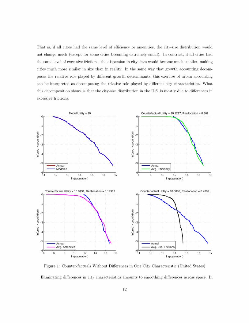
That is, if all cities had the same level of efficiency or amenities, the city-size distribution would

not change much (except for some cities becoming extremely small). In contrast, if all cities had

the same level of excessive frictions, the dispersion in city sizes would become much smaller, making

cities much more similar in size than in reality. In the same way that growth accounting decom-

poses the relative role played by different growth determinants, this exercise of urban accounting

can be interpreted as decomposing the relative role played by different city characteristics. What

this decomposition shows is that the city-size distribution in the U.S. is mostly due to differences in

excessive frictions.

11 12 13 14 15 16 17-6

-5

-4

-3

-2

-1

0

ln(population)

ln(p

rob

> po

pula

tion)

Model Utility = 10

Counterfactuals Without One Shock, = 0.002 , = 0 , = 0

ActualModeled

6 8 10 12 14 16 18-6

-5

-4

-3

-2

-1

0

ln(population)

ln(p

rob

> po

pula

tion)

Counterfactual Utility = 10.1217, Reallocation = 0.367

ActualAvg. Efficiency

4 6 8 10 12 14 16 18-6

-5

-4

-3

-2

-1

0

ln(population)

ln(p

rob

> po

pula

tion)


ActualAvg. Amenities

11 12 13 14 15 16 17-6

-5

-4

-3

-2

-1

0

ln(population)

ln(p

rob

> po

pula

tion)


ActualAvg. Exc. Frictions

Figure 1: Counter-factuals Without Differences in One City Characteristic (United States)

Eliminating differences in city characteristics amounts to smoothing differences across space. In

12

the same way that the business cycle literature analyzes the welfare benefits of smoothing temporal

shocks, we can analyze the welfare effects of smoothing spatial shocks. As the numbers at the top of

the different panels in Figure 1 indicate, those welfare effects are modest: welfare would increase by

1.2% if all cities had the same efficiency, by 0.2% if all cities had the same amenities, and by 0.9% if

all cities had the same excessive frictions. Given the benchmark utility of u, in terms of consumption

equivalence, the corresponding figures would be, respectively, 12%, 2% and 9%. Finding positive

welfare effects, though modest, is not surprising. Eliminating differences across space tends to spread

people more equally across locations. Given that congestion costs increase with size in a convex way,

this leads to welfare gains. From a policy point of view, the modest welfare gains from smoothing we

find should be interpreted, if anything, as upper bounds. Indeed, completely eliminating differences is

probably impossible, given that some of a city’s characteristics may be given by nature or geography

and thus difficult to change or amend. In addition, our counter-factual exercises assume people can

move across locations at no cost.

Spatial smoothing can often be reinterpreted as a size-dependent policy, thus affecting the fate of

mega-cities relative to medium-sized and smaller cities. For example, Figure 1 shows that equalizing

efficiency makes the city-size distribution slightly less disperse: the larger cities become smaller and

the smaller cities become larger. For example, Los Angeles would lose 29% of its population. The

respective figures for New York and Chicago would be losses of 77% and 46%. Since it reduces the

dispersion of the city-size distribution, a policy that smooths efficiency differences is a size-dependent

policy. It improves efficiency in smaller cities relative to larger cities. The same size-dependency

is present when equalizing differences in excessive frictions. In contrast, amenities are less strongly

correlated with size. For example, when equalizing amenities across locations, some of the larger

cities would lose (Los Angeles and San Diego would lose 8% and 42% of their populations), whereas

others would gain (New York and Philadelphia would increase their populations by 44% and 39%).

Although smoothing differences in efficiency and amenities has a limited effect on the city-size dis-

tribution (the counter-factual distribution and the actual distribution do not look all that different),

the examples of the individual cities mentioned above illustrate that the ordering of cities changes

substantially. For instance, when equalizing efficiency across all cities, New York is no longer the

country’s mega-city and drops to 6th position, overtaken by cities such as Riverside, Los Angeles,

Chicago and Phoenix. The country’s mega-city is now Riverside, with a population very similar to

New York’s actual population. This reordering of cities implies that behind the veil of an apparently

stable city-size distribution, there would be substantial reallocation of population. When calculating

13

reallocation following the methodology of Davis and Haltiwanger (1992) by adding the number of

new workers in expanding cities as a proportion of total population, we find a reallocation of 37%

when we eliminate differences in efficiency. The corresponding figures when eliminating differences

in amenities and excessive frictions are, respectively, 20% and 44%. (These reallocation numbers are

given at the top of each panel in all figures.) At this point it is important to recall that the welfare

differences from smoothing are computed under the assumption of free mobility. If one were to take

into account the costs of moving and the magnitude of reallocation, it is likely that any modest

positive welfare gain from smoothing would vanish.

3.4. China

Figure 2 represents the results of smoothing differences in city characteristics for the case of China.3

The most striking difference with the U.S. is that the welfare effects are orders of magnitude larger.

If all Chinese cities had the same level of efficiency, welfare would increase by 55%, and if all had

the same level of amenities, welfare would increase by 13%. In terms of consumption equivalence,

the respective numbers are much larger. These figures suggest that smoothing out differences in

efficiency and amenities could have enormous effects on China’s welfare. This is consistent with the

view that the Chinese economy is plagued by important regional disparities.

In terms of how spatial smoothing affects larger cities, we find that Beijing and Shanghai would

lose about 97% of their populations if we equalize efficiency. In contrast, if we equalize amenities,

Beijing would lose 10% of its population while Shanghai would lose only 2%. Does this imply that

smoothing out differences would lead to the demise of China’s mega-cities? Not necessarily. In

fact, as Figure 2 indicates, eliminating differences in efficiency or amenities would make the city-size

distribution more dispersed, implying that China’s largest cities would become larger and China’s

smallest cities would become smaller.

In contrast to the U.S., where smoothing efficiency made cities more equal in size, in China

the opposite happens. Given the huge decline in Beijing and Shanghai, this may seem somewhat

counter-intuitive. What happens is that some of the medium-sized cities with high amenities and low

efficiency now become the new mega-cities, and they end up being larger than present-day Beijing and

3There is one difference with the exercise we perform for the U.S. When eliminating differences in a city charac-

teristic, we set it equal to the median, rather than the weighted mean, of all cities. This change underestimates the

difference between China and the U.S. We do this differently because the weighted mean of Chinese city TFP would

make cities so productive that an equilibrium with the same number of cities does not exist.

14

Shanghai. The country’s two largest cities become Liuan in Anhui province (population 38 million)

and Bazhong in Sichuan province (population 31 million). These are cities with high amenities but

dismal productivity. Keeping those amenities constant and giving them median productivity would

transform them into huge cities.

12 13 14 15 16 17-6

-5

-4

-3

-2

-1

0

ln(population)

ln(p

rob

> po

pula

tion)

Model Utility = 10

China: Counterfactuals Without One Shock, = 0.001 , = 0 , = 0

ActualModeled

8 10 12 14 16 18-6

-5

-4

-3

-2

-1

0

ln(population)

ln(p

rob

> po

pula

tion)



8 10 12 14 16 18-6

-5

-4

-3

-2

-1

0

ln(population)

ln(p

rob

> po

pula

tion)



12 13 14 15 16 17-6

-5

-4

-3

-2

-1

0

ln(population)

ln(p

rob

> po

pula

tion)



Figure 2: Counter-factuals Without Differences in One City Characteristic (China)

The other finding — equalizing amenities leads to greater dispersion of the city-size distribution

— is the result of many of the larger cities in China having poor amenities. One probable reason for

this are formal and informal migratory restrictions in the past and present. Indeed, if large cities are

kept artificially small through mobility restrictions, this will show up as low amenities in our model.

Take the case of a highly efficient city with a predicted city size larger than observed in reality. In

15

that case, some other force in our model must keep it from reaching that larger size. Given our

identification strategy for the different city determinants (Step 4), that counteracting force will be

worse amenities. As a result, many of the highly efficient eastern coastal cities have low amenities.

Giving them average amenities would make them grow tremendously. This is the case, for example,

of several of the cities of Guangdong province, which constituted some of the first special economic

zones under Deng Xiaoping’s Open Door Policy. Shenzhen would grow to a population of 78 million,

and Guangzhou would increase its population by 72%. This finding is in line with Au and Henderson

(2006), who argue that China’s mega-cities are too small. As is well known, migratory restrictions

are not applied always and everywhere in China. The World Development Report 2009 gives the

example of the cities of Chongqing and Chengdu, which are pursuing “an unabashedly urbanization-

based growth strategy” (p.#221). If those cities are benefiting from government policies promoting

rural-urban migration, then this should be reflected in our model as high amenities. Consistent with

this, if those cities had average amenities, Chongqing would lose 98% of its population and Chengdu

a more modest but still high 66%.

Although mobility restrictions often stem from government policy through the so-called hukou

system, not all such restrictions are policy-based. Cities take time to grow, housing needs to be con-

structed, and other urban infrastructure needs to be built. The “time to build” implies that Chinese

cities can only gradually converge to their steady-state population level. The city of Shenzhen is

telling in this context: while the model predicts that it is much too small, it is unclear which part is

due to policy restrictions and which part is due to the “time to build” constraint. Given that it has

been China’s fastest growing city since 1979 (WDR 2009), it might very well not have been able to

grow much faster, even if people had been completely free to move.

Other urban problems that afflict many mega-cities, but more so in China than in the U.S., include

severe air pollution. Again, in our model such pollution will show up as a negative amenity, making

cities such as Beijing less desirable places to reside. In that sense, the low amenities of the larger

Chinese cities might also be due to environmental problems.

Overall we find that a more equal distribution of amenities or efficiency would lead to larger

cities and huge welfare gains. Greater mobility would surely contribute to narrowing the dispersion

in amenities, allowing the larger cities to grow further. Differences in efficiency are also bound

to become smaller over time, as technology and efficient management practices diffuse spatially.

Comparing the spatial distribution of efficiency in China and the U.S. is illustrative: taking the

standard deviation of the log of efficiency as a measure of dispersion, in China it stands at 0.33,

16

double the value of that in the U.S. This explains in part the much larger welfare gains from

smoothing efficiency across cities in China compared to the U.S.

3.5 Mexico

From the point of view of the relative importance of the different determinants of the city-size

distribution, the results for Mexico in Figure 3 show a country that is somewhat in between the U.S.

and China. Both the distribution of efficiency (as in China) and the distribution of excessive frictions

(as in the U.S.) seem to play a significant role. In contrast, from the point of view of welfare, Mexico

looks very much like the U.S. and very different from China. Eliminating differences in efficiency,

amenities and excessive frictions increases utility by, respectively, 0.7%, 1.1% and 1.2%. In terms

of consumption equivalence, those numbers correspond to, respectively, 7%, 11% and 12%. These

modest effects, compared to China, suggest that Mexico suffers less from mobility restrictions than

China. This result also seems to imply that differences across cities are less pronounced in Mexico

than in China, implying that equalizing characteristics has less of an effect.

Another relevant question is how spatial smoothing affects mega-cities relative to medium-sized

and smaller cities. In the case of efficiency, we found that smoothing differences made the city-

size distribution slightly less disperse in the U.S. but more disperse in China. Mexico fits neither

case. As can be seen in Figure 3, for the exercise when we equalize efficiency (upper-right panel),

the intermediate-sized cities become larger, the smaller cities become smaller, but the country’s

mega-city, Mexico City, becomes smaller. To be exact, Mexico City loses 78% of its population,

dropping from 19.2 million to 4.3 million. But, in contrast to the U.S., no other city takes its place.

Instead, some of the intermediate-sized cities now become substantially larger, without reaching the

dimensions of Mexico City. This is the case of Leon, with a population that increases from 1.4 to

5.8 million and becomes the country’s largest city. Other examples of medium-sized cities gaining

include Puebla (60%), Aguascalientes (136%) and Acapulco (621%). The latter example can be

easily understood: Acapulco has one of the country’s highest amenities, so that once it gets the

country’s average efficiency, it grows tremendously.

When equalizing amenities across cities, the effect is quite different. In that case, many of the

larger cities would lose population, such as Puebla (-96%), but not Mexico City, which would grow

from 19.2 million to 27.2 million, and Tijuana, which would increase its residents from 1.5 million

to 7.2 million. This reflects those latter cities having bad amenities. Once again, it is important to

17

understand that our identification strategy implies that amenities should be interpreted in a broad

sense. For example, any feature that holds back city growth but that does not distort the labor

supply is assigned to amenities. For example, if pollution and a complex geography puts the brakes

on the growth of Mexico City, this will show up as a negative amenity.

11 12 13 14 15 16 17−4

−3.5

−3

−2.5

−2

−1.5

−1

−0.5

0

ln(population)

ln(p

rob

> po

pula

tion)

Model Utility = 10

Counterfactuals Without One Shock, g = 0.0015566 , t = 0 , c = 0

ActualModeled

8 10 12 14 16 18−4

−3.5

−3

−2.5

−2

−1.5

−1

−0.5

0

ln(population)

ln(p

rob

> po

pula

tion)



4 6 8 10 12 14 16 18−4

−3.5

−3

−2.5

−2

−1.5

−1

−0.5

0

ln(population)

ln(p

rob

> po

pula

tion)



10 11 12 13 14 15 16 17−4

−3.5

−3

−2.5

−2

−1.5

−1

−0.5

0

ln(population)

ln(p

rob

> po

pula

tion)



Figure 3: Counter-factuals Without Differences in One City Characteristic (Mexico)

Until now we have compared urban systems across countries, but obviously our methodology can

easily be applied to compare urban systems across time. In Table 3 we compare the welfare changes

from smoothing differences in city characteristics in four different years: 1989, 1994, 2000 and 2005.

In the case of efficiency we see welfare gains rising from 1.1% in 1989 to 2.6% in 1994, and then

dropping again to 2.2% in 2000 and 0.4% in 2005. For the other characteristics, that pattern is

18

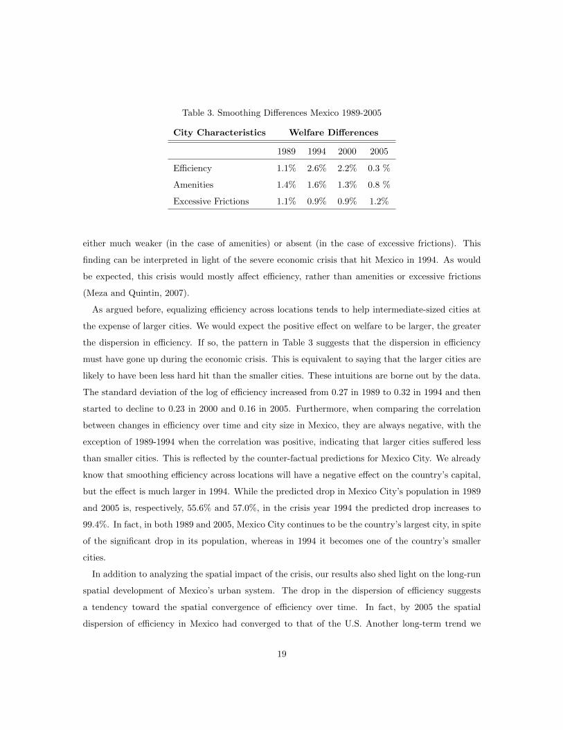
Table 3. Smoothing Differences Mexico 1989-2005

City Characteristics Welfare Differences

1989 1994 2000 2005

Efficiency 1.1% 2.6% 2.2% 0.3 %

Amenities 1.4% 1.6% 1.3% 0.8 %

Excessive Frictions 1.1% 0.9% 0.9% 1.2%

either much weaker (in the case of amenities) or absent (in the case of excessive frictions). This

finding can be interpreted in light of the severe economic crisis that hit Mexico in 1994. As would

be expected, this crisis would mostly affect efficiency, rather than amenities or excessive frictions

(Meza and Quintin, 2007).

As argued before, equalizing efficiency across locations tends to help intermediate-sized cities at

the expense of larger cities. We would expect the positive effect on welfare to be larger, the greater

the dispersion in efficiency. If so, the pattern in Table 3 suggests that the dispersion in efficiency

must have gone up during the economic crisis. This is equivalent to saying that the larger cities are

likely to have been less hard hit than the smaller cities. These intuitions are borne out by the data.

The standard deviation of the log of efficiency increased from 0.27 in 1989 to 0.32 in 1994 and then

started to decline to 0.23 in 2000 and 0.16 in 2005. Furthermore, when comparing the correlation

between changes in efficiency over time and city size in Mexico, they are always negative, with the

exception of 1989-1994 when the correlation was positive, indicating that larger cities suffered less

than smaller cities. This is reflected by the counter-factual predictions for Mexico City. We already

know that smoothing efficiency across locations will have a negative effect on the country’s capital,

but the effect is much larger in 1994. While the predicted drop in Mexico City’s population in 1989

and 2005 is, respectively, 55.6% and 57.0%, in the crisis year 1994 the predicted drop increases to

99.4%. In fact, in both 1989 and 2005, Mexico City continues to be the country’s largest city, in spite

of the significant drop in its population, whereas in 1994 it becomes one of the country’s smaller

cities.

In addition to analyzing the spatial impact of the crisis, our results also shed light on the long-run

spatial development of Mexico’s urban system. The drop in the dispersion of efficiency suggests

a tendency toward the spatial convergence of efficiency over time. In fact, by 2005 the spatial

dispersion of efficiency in Mexico had converged to that of the U.S. Another long-term trend we

19

observe is the worsening in Mexico City’s amenities. If the country’s capital had the country’s

average level of amenities, it would have lost 41.7% of its population in 1989. By 2005 the situation

was completely reversed: with average amenities, the city would gain 40.0% in population.

4. WHAT DID WE LEARN?

In this chapter we have shown how a simple general equilibrium model of a system of cities can be

implemented to quantitatively analyze how size-dependent policies affect the importance of mega-

cities relative to intermediate-sized and smaller cities. For example, if cities became more equal in

their efficiency, mega-cities would lose in the U.S. but would gain in China. Intuitively, because

congestion costs rising with city size, one would expect larger cities to lose when efficiency becomes

more equally spread in space. The fact that this does not happen in China illustrates the importance

of analyzing these questions in a general equilibrium framework. In China, some of the intermediate-

sized cities have good amenities but dismal productivity, so that equalizing productivity across cities

allows them to grow into huge mega-cities. We have also uncovered indirect evidence of mobility

restrictions in China, problems that do not seem to be present in the U.S. or Mexico.

When discussing the welfare gains from policies that spread efficiency or amenities more equally

across space, those should typically be interpreted as upper bounds. Not only are there costs implied

by moving people across cities, but more important, policy may not always be able to reduce spatial

differences even if it wanted to. The success of Shenzhen, for example, though partly policy driven,

has much to do with its geographic location, next to Hong Kong and well connected to global

manufacturing production networks. Investment in infrastructure and connectivity to the outside

world may help the lagging cities in the West of China but are unlikely to do away with their less

desirable geographic location.

The framework we presented can easily incorporate additional features, such as externalities in

both efficiency and amenities. In the case of efficiency, allowing for externalities tends to lower

the cost of mega-cities, so policies that reduce differences across space are likely to have smaller

welfare effects. In the case of amenities, the answer is more complex, because it depends on whether

amenities become better or worse when city size increases (consumption amenities would improve,

but pollution or crime would probably worsen). Though we have mainly focused on the policy of

more evenly spreading efficiency or amenities, it is of course possible to analyze the welfare effects

of other policies, such as restricting mobility across cities or subsidizing or taxing a particular set of

20

cities (or even a single one).

The important lesson is that much is to be learned from a quantitative analysis of urban systems.

Analyzing policy interventions for just one city, without taking into account its effects on other

cities, is likely to be misleading. The same problem may arise when focusing exclusively on one

of the determinants of the city-size distribution. Analyzing the effect of reducing productivity

differences across space, without taking into account that cities have other characteristics, such as

amenities, will lead to wrong conclusions. By having presented a guide of how a general equilibrium

analysis of urban systems can be implemented, our hope is that this will provide a useful tool for

policy makers in different countries.

REFERENCES

[1] Au, C.-C. and Henderson, J.V., 2006. “Are Chinese Cities Too Small?,” Review of Economic Studies,

73, 549-576.

[2] Bai, C.-E., Hsieh, C.-T. and Qian, Y., 2006. “The Return to Capital in China,” Brookings Papers

on Economic Activity, 37, 61-102.

[3] Davis, S.J. and Haltiwanger, J., 1992. “Gross Job Creation, Gross Job Destruction, and Employment

Reallocation,” Quarterly Journal of Economics, 107, 819-63.

[4] Desmet, K. and Rossi-Hansberg, E., 2012. “Urban Accounting and Welfare,” unpublished.

[5] Kehoe, T. and Ruhl, J.R., 2010. “Why Have Economic Reforms in Mexico Not Generated Growth?,”

Journal of Economic Literature, 48, 1005-27.

[6] McGrattan, E. and Prescott, E., 2009. “Unmeasured Investment and the Puzzling U.S. Boom in the

1990s,” Research Department Staff Report 369, Federal Reserve Bank of Minneapolis.

[7] Meza, F. and Quintin, E., 2007. “Factor Utilization and the Real Impact of Financial Crises,” B.E.

Journal of Macroeconomics, 7 (Advances), Article 33.

[8] UN-Habitat, 2010. The State of African Cities 2010: Governance, Inequality and Urban Land Mar-

kets.

[9] Restuccia, D. and Rogerson, R., 2008. “Policy Distortions and Aggregate Productivity with Hetero-

geneous Plants,” Review of Economic Dynamics, 11, 707-720.

21

[10] World Development Report 2009: Reshaping Economic Geography, World Bank, Washington D.C.

22

Documents

Analyzing Urban Systems: Have Mega-Cities Become …erossi/WBGlaeser040412.pdf · Analyzing Urban Systems: Have Mega-Cities Become Too Large? Klaus Desmet Universidad Carlos III Esteban