Analyzing the Rate at Which Languages Lose the Inﬂuence of

Cognitive Science 38 (2014) 1406–1431Copyright © 2014 Cognitive Science Society, Inc. All rights reserved.ISSN: 0364-0213 print / 1551-6709 onlineDOI: 10.1111/cogs.12112

Analyzing the Rate at Which Languages Lose theInfluence of a Common Ancestor

Anna N. Rafferty,a Thomas L. Griffiths,b Dan Kleina

aComputer Science Division, University of California, BerkeleybDepartment of Psychology, University of California, Berkeley

Received 14 March 2012; received in revised form 18 June 2013; accepted 1 July 2013

Abstract

Analyzing the rate at which languages change can clarify whether similarities across languages

are solely the result of cognitive biases or might be partially due to descent from a common

ancestor. To demonstrate this approach, we use a simple model of language evolution to mathe-

matically determine how long it should take for the distribution over languages to lose the influ-

ence of a common ancestor and converge to a form that is determined by constraints on language

learning. We show that modeling language learning as Bayesian inference of n binary parameters

or the ordering of n constraints results in convergence in a number of generations that is on the

order of n log n. We relax some of the simplifying assumptions of this model to explore how dif-

ferent assumptions about language evolution affect predictions about the time to convergence; in

general, convergence time increases as the model becomes more realistic. This allows us to char-

acterize the assumptions about language learning (given the models that we consider) that are suf-

ficient for convergence to have taken place on a timescale that is consistent with the origin of

human languages. These results clearly identify the consequences of a set of simple models of lan-

guage evolution and show how analysis of convergence rates provides a tool that can be used to

explore questions about the relationship between accounts of language learning and the origins of

similarities across languages.

Keywords: Iterated learning; Language evolution; Convergence bounds

1. Introduction

Human languages share a surprising number of properties, ranging from high-level

characteristics such as compositional mapping between sound and meaning to relatively

low-level syntactic regularities (Comrie, 1981; Greenberg, 1963; Hawkins, 1988). One

Correspondence should be sent to Anna N. Rafferty, Computer Science Division, University of California,

Berkeley, CA 94720. E-mail: [email protected]

explanation for these universal properties is that they reflect constraints on human

language learning, with the mechanisms by which we acquire language only allowing us

to learn languages with these properties (Chomsky, 1965). These mechanisms may also

make certain languages more learnable than others, resulting in linguistic trends that favor

particular properties (Krupa, 1982; Tily, Frank, & Jaeger, 2011). However, similarities

across languages could also be partially the result of descent from a common ancestor

(Bengtson & Ruhlen, 1994; Greenberg, 2002). While the theory of a common origin is

controversial (Picard, 1998), recent work on phonemic diversity across languages has lent

support to this theory (Atkinson, 2011), and there is evidence that some linguistic pat-

terns, such as trends in word order, can be explained by lineage patterns in language evo-

lution and that these patterns allow one to glean information about a common ancestral

language (Dunn, Greenhill, Levinson, & Gray, 2011; Gell-Mann & Ruhlen, 2011).

Given that both a common ancestor and learning biases may contribute to similarities

across languages, we wish to investigate how quickly the influence of a common ancestor

is lost in the process of language evolution. As languages evolve, learning biases will

become the dominant cause of similarities across different languages, and the influence of

the common ancestor will eventually disappear. Modeling the process of language change

makes it possible to determine how different assumptions about language evolution affect

the rate at which this influence will dissipate. We demonstrate how this approach can be

used, providing bounds on how quickly the influence of a common ancestor will disap-

pear in a simple model of language evolution. This allows us to identify assumptions

about language learning (within this simple model) that result in bounds that are consis-

tent with the origin of human languages. We then investigate how relaxing the simplifica-

tions of this model affects the rate of language change, and find that the relaxations tend

to slow the rate at which the influence of the common ancestor is lost. These results pro-

vide a clear picture of the implications of the simple models that we consider, but more

important, they illustrate a methodology that can be applied to determine the implications

of more complex and realistic models of language learning and language evolution.

Language transmission is a process in which those who are currently learning a lan-

guage do so based on the utterances of other members of the population. These other

members were also once language learners. Building on recent formal models of language

evolution (Griffiths & Kalish, 2007; Kirby, 2001; Kirby, Smith, & Brighton, 2004; Kirby,

Dowman, & Griffiths, 2007; Smith, Kirby, & Brighton, 2003) that share this feature of

current learners learning from previous learners, the models we consider are based on

iterated learning. Iterated learning models assume that each generation of people learns

language from utterances generated by the previous generation. By modeling how lan-

guages change over many generations of transmission, the iterated learning framework

provides an opportunity to examine how constraints on learning influence the process of

language transmission. We begin by analyzing an iterated learning model that makes

strong simplifying assumptions, such as a lack of interaction between learners in the same

generation, allowing us to obtain analytic results quantifying how quickly languages lose

the influence of an ancestor.1 The language of the initial generation is modeled as known,

and each future generation has a distribution over possible languages. Previous research

A. N. Rafferty, T. L. Griffiths, D. Klein / Cognitive Science 38 (2014) 1407

using this model has shown that after some number of generations, the distribution over

languages converges to an equilibrium that reflects the constraints that guide learning

(Griffiths & Kalish, 2007). After convergence, the behavior of learners is independent of

the language spoken by the first generation. Prior to convergence, similarities across lan-

guages may reflect common ancestry. Our key contribution is providing asymptotic

bounds on the number of generations required for convergence, known as the convergencetime, which we obtain by analyzing Markov chains associated with iterated learning.

Bounding the convergence time of iterated learning is a step toward understanding

whether similarities across languages are solely caused by constraints on learning or

whether a common ancestor might also be contributing to these similarities. To bound the

number of generations required for iterated learning to converge, we need to make some

assumptions about the algorithms and representations used by learners. Following previ-

ous analyses (Griffiths & Kalish, 2007; Kirby et al., 2007), we assume that learners

update their beliefs about the plausibility of a set of linguistic hypotheses using Bayesian

inference. We outline how this approach can be applied in a simple model inspired by

the Principles and Parameters framework (Chomsky & Lasnik, 1993; Gibson & Wexler,

1994; Niyogi & Berwick, 1996). In this model, grammars are represented as vectors of

binary parameter values. We show that iterated learning with a uniform prior reaches

equilibrium after a number of generations that is on the order of n log n, where n is the

number of parameters.

By using a Principles and Parameters framework, our analysis assumes a finite hypoth-

esis space where all languages can be represented using the same parameters. The conver-

gence analysis is a tool for determining whether the ancestor language has an influence

on descendant languages beyond this common representation. If it does not, then we

could use the observed distribution over one of these parameters (e.g., word order) to

draw conclusions about cognitive biases. Conversely, if the common ancestor still has an

effect, we cannot draw strong conclusions about human biases based on this distribution,

as there is a danger of underestimating the amount of variation that needs to be accounted

for (such as the number of parameters required to represent the space of possible lan-

guages). Pairing the Principles and Parameters iterated learning model with data concern-

ing the estimated amount of time since the origin of human languages, the number of

parameters, and the rate of language change, we find that under this model it is possible

that a common ancestor language (or languages) could still have some influence on simi-

larities across modern languages.

The initial model makes a number of simplifying assumptions about the process of

language transmission. As previously mentioned, we address the key simplifications by

determining how the predictions of the model change when these assumptions are

relaxed. These relaxations include using another formal model of language acquisition,

inspired by Optimality Theory (Prince & Smolensky, 2004); modifying the assumed

probability of different languages; allowing the parts of a language to change at different

rates; incorporating learning from multiple previous generations; and including

differential transmission of languages based on communicative success. All of these

variations either reproduce our original results, or slow down convergence, in some cases

1408 A. N. Rafferty, T. L. Griffiths, D. Klein / Cognitive Science 38 (2014)

dramatically. Considering this wider range of models thus reinforces our original

conclusion—that under simple accounts of language learning it remains possible that a

common ancestor could play a role in explaining trends across modern languages. These

more comprehensive analyses also reinforce our methodological goal of showing how

analysis of convergence rates can contribute to debates about the causes of similarities

across languages, illustrating the steps that can be taken towards determining the conver-

gence rates of more realistic models of language evolution.

2. A simple model of language learning and transmission

To illustrate how convergence rates can be determined for models of language evolu-

tion, we focus on a simple model of language learning and transmission. This model has

two parts: how language transmission occurs, and the nature of language learning. This

section presents these two parts of the model in turn.

2.1. Transmission by iterated learning

Iterated learning has been used to model many aspects of language evolution, provid-

ing a simple way to explore the effects of cultural transmission on the structure of lan-

guages (Griffiths & Kalish, 2007; Kirby, 2001; Kirby et al., 2004, 2007; Smith et al.,

2003). The basic assumption behind the model—that each learner learns from somebody

who was herself a learner—captures a phenomenon we see in nature: Parents pass on lan-

guage to their children, and these children in turn pass on language to their own children.

The sounds the children hear are the input, and the child produces language (creates out-

put) by combining this input with whatever constraints guide learning.

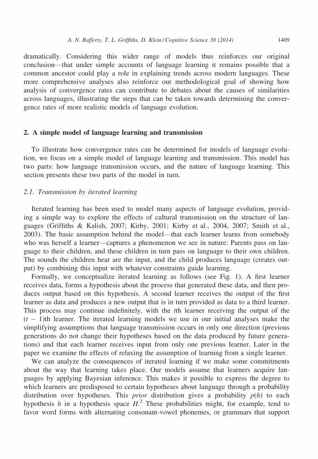
Formally, we conceptualize iterated learning as follows (see Fig. 1). A first learner

receives data, forms a hypothesis about the process that generated these data, and then pro-

duces output based on this hypothesis. A second learner receives the output of the first

learner as data and produces a new output that is in turn provided as data to a third learner.

This process may continue indefinitely, with the tth learner receiving the output of the

(t � 1)th learner. The iterated learning models we use in our initial analyses make the

simplifying assumptions that language transmission occurs in only one direction (previous

generations do not change their hypotheses based on the data produced by future genera-

tions) and that each learner receives input from only one previous learner. Later in the

paper we examine the effects of relaxing the assumption of learning from a single learner.

We can analyze the consequences of iterated learning if we make some commitments

about the way that learning takes place. Our models assume that learners acquire lan-

guages by applying Bayesian inference. This makes it possible to express the degree to

which learners are predisposed to certain hypotheses about language through a probability

distribution over hypotheses. This prior distribution gives a probability p(h) to each

hypothesis h in a hypothesis space H.2 These probabilities might, for example, tend to

favor word forms with alternating consonant-vowel phonemes, or grammars that support


constituent structure. These constraints on learning are combined with data via Bayesian

inference. The posterior distribution over hypotheses given data d is given by Bayes’

rule,

pðhjdÞ ¼ pðdjhÞpðhÞPh02H pðdjh0Þpðh0Þ ð1Þ

where the likelihood p(d|h) indicates the probability of seeing d under hypothesis h. We

assume that learners’ expectations about the distribution of the data given hypotheses are

consistent with the actual distribution (i.e., that the probability of the previous learner

generating data d from hypothesis h matches the likelihood function p(d|h)). Finally, weassume that learners choose a hypothesis by sampling from the posterior distribution,

although we consider other ways of selecting hypotheses later in this paper.3

The analyses we present in this paper are based on the observation that iterated

learning defines a Markov chain. A Markov chain is a sequence of random variables Xt

such that each Xt is independent of all preceding variables when conditioned on the

immediately preceding variable, Xt�1. The Markov chain is characterized by

the transition probabilities, pðxtjxt�1Þ. There are several ways of reducing iterated learning

to a Markov chain (Griffiths & Kalish, 2007). We will focus on the Markov chain

on hypotheses, where the sequence of random variables corresponds to the

hypotheses selected at each generation. The transition probabilities for this Markov chain

are obtained by summing over the data from the previous time step dt�1, with

pðhtjht�1Þ ¼ Pdt�1

pðhtjdt�1Þpðdt�1jht�1Þ (see Fig. 1).

Identifying iterated learning as a Markov chain allows us to draw on mathematical

results concerning the convergence of Markov chains. In particular, Markov chains can

converge to a stationary distribution, meaning that after some number of generations t,the marginal probability that a variable Xt takes value xt becomes fixed and independent

(A)

(B)

(C)

Fig. 1. Language evolution by iterated learning. (A) Each learner sees data, forms a hypothesis, and gener-

ates the data provided to the next learner. (B) The underlying stochastic process, with dt and ht being the data

generated by the tth learner and the hypothesis selected by that learner, respectively. (C) We consider the

Markov chain over hypotheses formed by summing over the data variables. All learners share the same prior

p(h), and each learner assumes the input data were created using the same p(d|h).


of the value of the first variable in the chain (Norris, 1997). Intuitively, the stationary dis-

tribution is a distribution over states in which the probability of each state is not affected

by further iterations of the Markov chain; in our case, the probability that a learner learns

a specific language at time t is equal to the probability of any future learner learning that

language. The stationary distribution is thus an equilibrium that iterated learning will

eventually reach, regardless of the hypothesis of the first learner, provided simple techni-

cal conditions are satisfied (for details, see Griffiths & Kalish, 2007).

Previous work has shown that the stationary distribution of the Markov chain defined

by Bayesian learners sampling from the posterior is the learners’ prior distribution over

hypotheses, p(h) (Griffiths & Kalish, 2007). This result illustrates how constraints on

learning can influence the languages that people come to speak, indicating that iterated

learning will converge to an equilibrium that is determined by these constraints and inde-

pendent of the language spoken by the first learner in the chain. However, characterizing

the stationary distribution of iterated learning still leaves open the question of whether

enough generations of learning have occurred for convergence to this distribution to have

taken place in human languages. Previous work has identified factors influencing the rate

of convergence in very simple settings (Griffiths & Kalish, 2007). Our contribution is to

provide analytic upper bounds on the convergence time of iterated learning with simple

representations of the structure of a language that are consistent with linguistic theories.

2.2. Bayesian learning of linguistic parameters

Defining a Bayesian model of language learning requires choosing a representation of

the structure of a language. In this section, we outline a Bayesian model of language learn-

ing inspired by the Principles and Parameters theory (Chomsky & Lasnik, 1993), a pro-

posal for how to characterize a Universal Grammar that captured all learnable languages.

Under this theory, all languages are assumed to be representable using only a small num-

ber of parameterized principles, with the values of the parameters being set through expo-

sure to language. This places strong constraints on the space of possible languages,

downplaying the role of learning in language acquisition. These strong constraints provide

one reason to use this as a starting point for our investigation of the rate of convergence of

iterated learning: We might expect that reducing the space of possible languages to a finite

discrete set would mean that convergence occurs quickly, giving us a bound on conver-

gence for richer representations of the space of possible languages. Bayesian models of

language learning consistent with other linguistic theories are also possible, and we con-

sider the effect of adopting different theoretical approaches later in the paper.

The Principles and Parameters theory postulates that all languages follow a finite set of

principles, with specific languages defined by setting the values of a finite set of parame-

ters (Chomsky & Lasnik, 1993). For example, one parameter might encode the head

directionality of the language (with the values indicating left- or right-headedness), while

another might encode whether covert subjects are permitted. We will assume that parame-

ters are binary, as in previous models of language acquisition based on Principles and

Parameters (Gibson & Wexler, 1994; Niyogi & Berwick, 1996). Learning a language is


learning the settings for these parameters. In reality, learning is not an instantaneous pro-

cess. Learners are presented with a series of examples from the target language and may

change their parameters after each example. The exact model of learning varies based on

assumptions about the learners’ behavior (e.g., Gibson & Wexler, 1994; Niyogi & Ber-

wick, 1996). We do not model this fine-grained process, but rather lump acquisition into

one computation, wherein a single hypothesis h is selected on the basis of a single data

representation d.To specify a Bayesian learner for this setting, we define a hypothesis space H, a data

representation space D, a prior distribution p(h), and a likelihood p(d|h). Assuming a set

of n binary parameters, our hypothesis space is composed of all binary vectors of length

n: H = {0,1}n. We represent the data space as strings in {0,1,?}n, where 0 and 1 indicate

the values of parameters that are fully determined by the evidence and question marks

indicate underdetermined parameters. For now, we assume a uniform prior, with p(h) = 1/2n for all h 2 H. To define the likelihood, we assume the data given to each

generation fully specify all but m of the n parameters, with the m unknown parameters

chosen uniformly at random without replacement. Then, p(d|h) is zero for all strings dwith a 0 or 1 not matching the binary vector h or that do not have exactly m question

marks (i.e., those consistent with h). Moreover, we assume that p(d|h) is equal for all

strings consistent with h. There arenm

� �strings consistent with any hypothesis, so

pðdjhÞ ¼ m!ðn�mÞ!n! for all d consistent with h (see Fig. 2).

Applying Bayes’ rule (Eq. 1) using this hypothesis space and likelihood, the posterior

distribution is

pðhjdÞ ¼pðhÞP

h0 :h0‘d pðh0Þh ‘ d

0 otherwise

8<: ð2Þ

where h ⊢ d indicates that h is consistent with d. This follows from the fact that p(d|h) isconstant for all h such that h ⊢ d, meaning that the likelihood cancels from the numerator

and denominator and the posterior is the prior renormalized over the set of consistent

hypotheses. For a uniform prior, the posterior probability of a consistent hypothesis is

simply the reciprocal of the number of consistent hypotheses. In the uniform case, 2m of

our hypotheses are valid, so pðhjdÞ ¼ 12m.

3. Convergence bounds

We now seek to bound the time to convergence of the Markov chain formed by iter-

ated learning. Bounds on the time to convergence are often expressed using total varia-tion distance. This is a distance measure between two probability distributions l and m on

some space Ω that is defined as kl � mk � 12

Px2X

jlðxÞ � mðxÞj ¼ maxA�X

jlðAÞ � mðAÞ


(Diaconis & Saloff-Coste, 1996). We seek to bound the rate of convergence of the distri-

butions of the h(t) to the stationary distribution, expressed via the number of iterations for

the total variation distance to fall below a small number ξ. This allows us to analytically

determine how many iterations the Markov chain must be run to conclude that the current

distribution is within ξ of the stationary distribution.

3.1. Asymptotic convergence bounds

To establish bounds on the convergence rate, we show that the Markov chains associ-

ated with iterated learning are reducible to Markov chains for which there are known

bounds. As described above, we assume each learner receives sufficient data to set all but

m of the n parameters in the hypothesis. We first consider the case where there is only

one unknown parameter (m = 1). In this case, each generation of iterated learning can

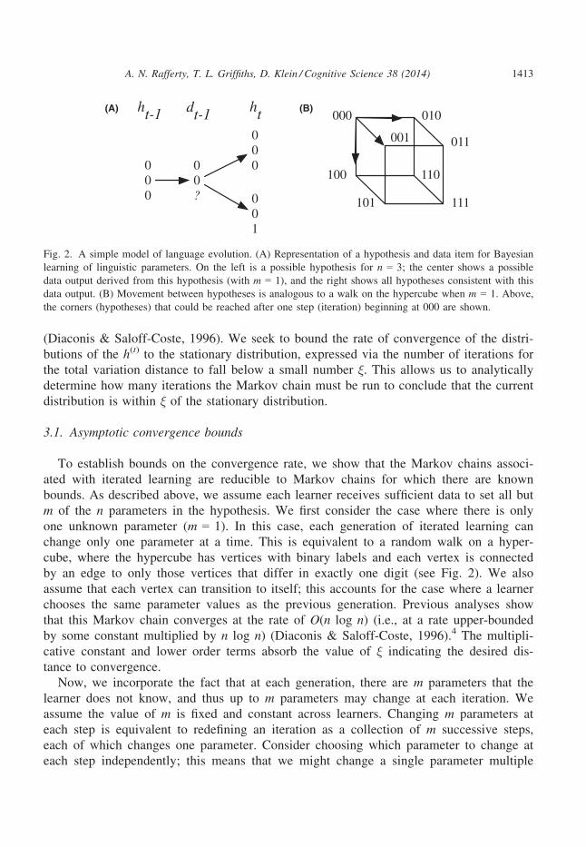
change only one parameter at a time. This is equivalent to a random walk on a hyper-

cube, where the hypercube has vertices with binary labels and each vertex is connected

by an edge to only those vertices that differ in exactly one digit (see Fig. 2). We also

assume that each vertex can transition to itself; this accounts for the case where a learner

chooses the same parameter values as the previous generation. Previous analyses show

that this Markov chain converges at the rate of O(n log n) (i.e., at a rate upper-bounded

by some constant multiplied by n log n) (Diaconis & Saloff-Coste, 1996).4 The multipli-

cative constant and lower order terms absorb the value of ξ indicating the desired dis-

tance to convergence.

Now, we incorporate the fact that at each generation, there are m parameters that the

learner does not know, and thus up to m parameters may change at each iteration. We

assume the value of m is fixed and constant across learners. Changing m parameters at

each step is equivalent to redefining an iteration as a collection of m successive steps,

each of which changes one parameter. Consider choosing which parameter to change at

each step independently; this means that we might change a single parameter multiple

000

00?

000

001

(A) (B)ht-1 dt-1 ht 000

100

010

111

001 011

110

101

Fig. 2. A simple model of language evolution. (A) Representation of a hypothesis and data item for Bayesian

learning of linguistic parameters. On the left is a possible hypothesis for n = 3; the center shows a possible

data output derived from this hypothesis (with m = 1), and the right shows all hypotheses consistent with this

data output. (B) Movement between hypotheses is analogous to a walk on the hypercube when m = 1. Above,

the corners (hypotheses) that could be reached after one step (iteration) beginning at 000 are shown.


times in one iteration. This process must converge in Oðnm log nÞ iterations, since each

iteration in which we can change up to m parameters is equivalent to m steps in our origi-

nal Markov chain. In our situation, however, we choose the m parameters without

replacement, so no parameter changes more than once per iteration. Since the net effect

of changing the same parameter twice in one iteration is similar to changing it once (from

the original value to the final value), changing m different parameters brings us at least

as close to convergence as changing fewer than m different parameters. Thus, the Markov

chain corresponding to our model converges in Oðnm log nÞ generations.

3.2. Simulation 1: Assessing the bounds

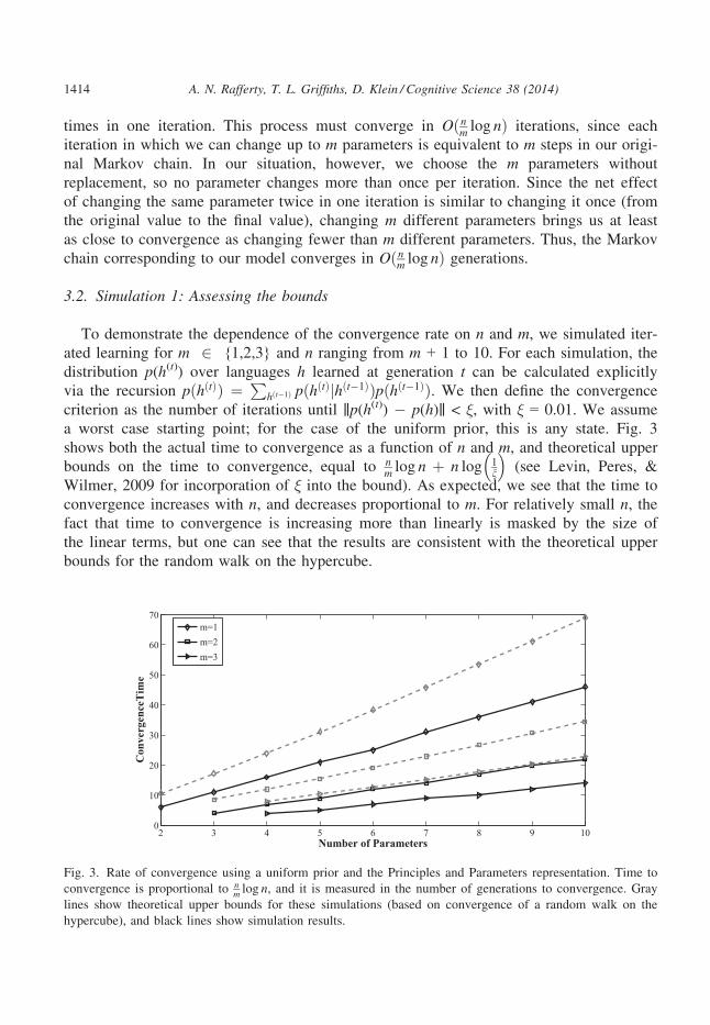
To demonstrate the dependence of the convergence rate on n and m, we simulated iter-

ated learning for m 2 {1,2,3} and n ranging from m + 1 to 10. For each simulation, the

distribution p(h(t)) over languages h learned at generation t can be calculated explicitly

via the recursion pðhðtÞÞ ¼ Phðt�1Þ pðhðtÞjhðt�1ÞÞpðhðt�1ÞÞ. We then define the convergence

criterion as the number of iterations until ‖p(h(t)) � p(h)‖ < ξ, with ξ = 0.01. We assume

a worst case starting point; for the case of the uniform prior, this is any state. Fig. 3

shows both the actual time to convergence as a function of n and m, and theoretical upper

bounds on the time to convergence, equal to nm log n þ n log 1

n

� �(see Levin, Peres, &

Wilmer, 2009 for incorporation of ξ into the bound). As expected, we see that the time to

convergence increases with n, and decreases proportional to m. For relatively small n, thefact that time to convergence is increasing more than linearly is masked by the size of

the linear terms, but one can see that the results are consistent with the theoretical upper

bounds for the random walk on the hypercube.

2 3 4 5 6 7 8 9 100

10

20

30

40

50

60

70

Number of Parameters

Con

verg

ence

Tim

e

m=1m=2m=3

Fig. 3. Rate of convergence using a uniform prior and the Principles and Parameters representation. Time to

convergence is proportional to nm log n, and it is measured in the number of generations to convergence. Gray

lines show theoretical upper bounds for these simulations (based on convergence of a random walk on the

hypercube), and black lines show simulation results.


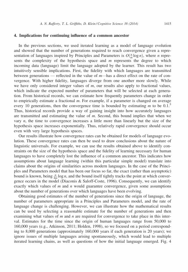
4. Implications for continuing influence of a common ancestor

In the previous sections, we used iterated learning as a model of language evolution

and showed that the number of generations required to reach convergence given a repre-

sentation of languages inspired by Principles and Parameters is Oðnm log nÞ, where n repre-

sents the complexity of the hypothesis space and m represents the degree to which

incoming data (language) limit the language adopted by the learner. This result has two

intuitively sensible implications. First, the fidelity with which languages are transmitted

between generations — reflected in the value of m—has a direct effect on the rate of con-

vergence. With higher fidelity, languages diverge from one another more slowly. While

we have only considered integer values of m, our results also apply to fractional values,

which indicate the expected number of parameters that will be selected at each genera-

tion. From historical records, we can estimate how frequently parameters change in order

to empirically estimate a fractional m. For example, if a parameter is changed on average

every 10 generations, then the convergence time is bounded by estimating m to be 0.1.5

Thus, historical records provide a way of gaining insight into how accurately languages

are transmitted and estimating the value of m. Second, this bound implies that when we

vary n, the time to convergence increases a little more than linearly but the size of the

hypothesis space increases exponentially. Thus, relatively rapid convergence should occur

even with very large hypothesis spaces.

Our results illustrate how convergence rates can be obtained for models of language evo-

lution. These convergence rates can then be used to draw conclusions about the nature of

linguistic universals. For example, we can use the results obtained above to identify con-

straints on the size of the hypothesis space and the fidelity of learning necessary for human

languages to have completely lost the influence of a common ancestor. This indicates how

assumptions about language learning (within this particular simple model) translate into

claims about the origins of similarities across modern languages. In the case of the Princi-

ples and Parameters model that has been our focus so far, the exact (rather than asymptotic)

bound is known, being n4m log n, and the bound itself tightly tracks the point at which conver-

gence occurs in the model (Diaconis & Saloff-Coste, 1996). Consequently, we can identify

exactly which values of m and n would guarantee convergence, given some assumptions

about the number of generations over which languages have been evolving.

Obtaining good estimates of the number of generations since the origin of language, the

number of parameters appropriate in a Principles and Parameters model, and the rate of

language change is challenging. However, we can illustrate how the mathematical results

can be used by selecting a reasonable estimate for the number of generations and then

examining what values of m and n are required for convergence to take place in this inter-

val. Estimates for the time since the origin of human languages range from 50,000 to

160,000 years (e.g., Atkinson, 2011; Holden, 1998), so we focused on a period correspond-

ing to 8,000 generations (approximately 160,000 years if each generation is 20 years); we

ignore issues of multiple languages arising spontaneously, which would lead to multiple

iterated learning chains, as well as questions of how the initial language emerged. Fig. 4


shows how times to convergence that fall within this interval vary given various plausible

values of m and n; note that this bound slightly underestimates the time to convergence

due to omitting terms of order lower than n. With small n and relatively large m, the graphsuggests that it is possible that language has been transmitted for a sufficient number of

generations to allow convergence; conversely, if m is much smaller or n is too high, the

figure suggests that language may not have existed for sufficient time to have converged.

Several authors have estimated the number of parameters that might be required for a

Principles and Parameters model; these estimates range from as low as 20 to as high as

50–100 parameters (Kayne, 2000; Lightfoot, 1999). With n = 20 parameters, the number

of parameters that changes each generation has to be m > 0.0019 to guarantee conver-

gence; n = 100 requires m > 0.014. We can also obtain an estimate for m by observing

the frequency of parameter changes in historical records, and we ask what values of n are

required for convergence. For example, Taylor (1994) found that ancient Greek changed

word orders over about 800 years, and Hroarsdottir (2000) provides evidence that it took

600–700 years for Icelandic word order to change. Such estimates provide a lower bound

on the time for a single parameter to be changed. The Greek word order occurred in

about 40 generations, and the Icelandic word order change took 30�35 generations.

These rates correspond to m = 0.025 and 0.029 � 0.033, respectively, implying that nwould have to be less than 158 and 177�201 for convergence to take place within 8,000

generations. Based on these values, it is plausible that human languages could have lost

the influence of a common ancestor. However, if the time language has existed is a bit

smaller than 8,000 generations, the actual number of parameters needed to define human

language a little larger than the estimates given above, or the rate of change a little

slower, then it could be the case that the influence of a common ancestor still affects the

similarities we see across languages.

00.2

0.40.6

0.81

0200

400600

8001000

0

2000

4000

6000

8000

Parameters dropped per generation (m)Number of parameters (n)

Gen

erat

ions

to c

onve

rgen

ce

Line shows where convergence time equals 8,000 generations

Fig. 4. Number of generations necessary for convergence, as a function of n and m. The surface is shown

for values that converge in 8,000 generations or fewer; the black line shows the two-dimensional projection

of values of m and n for which convergence is estimated at 8,000 generations. This corresponds to 160,000

years, with 20 years per generation, which is an upper limit on the maximum amount of time language may

have existed.


While the graph in Fig. 4 gives some understanding of how our analysis applies to

actual human languages, the model we have used is extremely simple. This model illus-

trates how the approach of bounding convergence rates can be useful to the debate about

the origins of linguistic universals, but drawing stronger conclusions will require consid-

ering more realistic models of language evolution. In the remainder of the paper we pro-

vide some preliminary steps in this direction, relaxing a number of the simplifying

assumptions in our model and assessing convergence time via simulation in order to

determine the effect that these assumptions have on convergence time.

5. Relaxing simplifying assumptions

We consider a variety of modifications to the assumptions of the original model to

ascertain how these assumptions contribute to our predictions about the rate of language

change. For each modification, further technical details can be found in the Appendix,

and simulation results are shown in Fig. 5.

5.1. Modifications to learning

The first class of changes to the model retain the basic structure of iterated learning but

modify the assumptions about how learning takes place. In these models we can still cal-

culate stationary distributions and determine the total variation distance in simulations.

(A) (B) (C)

(F)(E)(D)

Fig. 5. Effects of relaxing simplifying assumptions on time to convergence. (A) Optimality Theory represen-

tation: Results using this representation are similar to those for the Principles and Parameters representation.

(B) Entropy of prior distribution: As the entropy of the prior increases, indicating more uniformity, the time

to convergence decreases. (C) Entropy of the distribution of the probability of dropping each parameter of

the language vector: As the entropy of this distribution decreases, time to convergence increases dramatically.

(D) Population fitness model: Convergence time is relatively constant with increasing population size if an

additive fitness function is used, but it increases with a multiplicative fitness function. (E) Learning from mul-

tiple parents: As the number of parents increases, the time to convergence also increases. (F) Learning from

multiple generations: Showing a pattern very similar to that of learning from multiple parents, the time to

convergence increases with the number of generations from which the learner learns.


5.1.1. Optimality theoryTo determine whether linguistic representations other than Principles and Parameters

produce asymptotic convergence rates similar to our original results, we consider another

popular approach to modeling language learning. In Optimality Theory (OT), learning a

language is learning the rankings of various constraints (McCarthy, 2004; Prince & Smo-

lensky, 2004). These constraints are universal across languages and encode linguistic

properties. For example, one constraint might encode that high vowels follow high vow-

els. Whether a construction is well formed in a language is based on the ranking of the

constraints that the construction violates. Specifically, well-formed constructions are those

that violate the lowest-ranked constraints. Producing well-formed constructions thus

requires determining how constraints are ranked in the target language. As we prove in

the Appendix, using this linguistic representation gives the same asymptotic rate of con-

vergence as for the Principles and Parameters representation; Fig. 5(A) shows this result

in simulation.

5.1.2. Non-uniform priorsIn our model, we have assumed that all languages are considered equally likely by

learners. However, one might assume that there are certain languages that are easier to

learn than others, making some languages more probable a priori. We can examine the

effect of this assumption by changing the entropy of the prior distribution, that is, chang-

ing whether the prior makes all hypotheses equally likely or puts almost all weight on

only a few hypotheses. Our previous analyses show how convergence time varies with

the size of the hypothesis space, but non-uniform priors provide another way to model

constraints on learning that might influence convergence. We examine the effects of using

non-uniform priors by defining a distribution in which one language is designated a “pro-

totype,” and the probability of all other languages decreases with distance from this pro-

totype. As the entropy of the prior decreases, the upper bound on the time to

convergence increases (see the Appendix for details).

5.1.3 Choosing a hypothesis from the posteriorIn conducting our analyses, we assumed that learners sample from the posterior distri-

bution over hypotheses, but there are other psychologically plausible methods of select-

ing hypotheses from the posterior. Alternative methods of selecting a hypothesis, such

as selecting the hypothesis with the maximum posterior probability (MAP) and exponen-

tiated sampling, have been considered in previous work (Griffiths & Kalish, 2007; Kirby

et al., 2007). In the case of a uniform prior, both methods are equivalent to the sam-

pling method we considered since all hypotheses with non-zero probability have the

same probability in the uniform case; thus, our analyses of convergence time hold. In

the non-uniform case, exponentiated sampling is equivalent to a variation on the simula-

tion above concerning non-uniform priors (see the Appendix for details). For MAP in

the non-uniform case, convergence to the prototype hypothesis (that with the highest

probability in the non-uniform prior) will occur. The time in which this occurs is still

Oðnm log nÞ.6


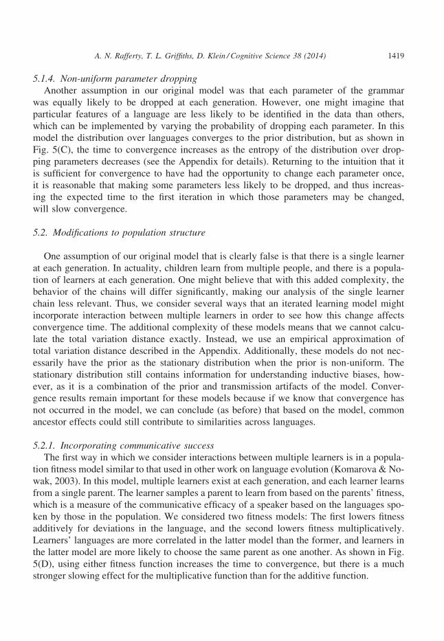
5.1.4. Non-uniform parameter droppingAnother assumption in our original model was that each parameter of the grammar

was equally likely to be dropped at each generation. However, one might imagine that

particular features of a language are less likely to be identified in the data than others,

which can be implemented by varying the probability of dropping each parameter. In this

model the distribution over languages converges to the prior distribution, but as shown in

Fig. 5(C), the time to convergence increases as the entropy of the distribution over drop-

ping parameters decreases (see the Appendix for details). Returning to the intuition that it

is sufficient for convergence to have had the opportunity to change each parameter once,

it is reasonable that making some parameters less likely to be dropped, and thus increas-

ing the expected time to the first iteration in which those parameters may be changed,

will slow convergence.

5.2. Modifications to population structure

One assumption of our original model that is clearly false is that there is a single learner

at each generation. In actuality, children learn from multiple people, and there is a popula-

tion of learners at each generation. One might believe that with this added complexity, the

behavior of the chains will differ significantly, making our analysis of the single learner

chain less relevant. Thus, we consider several ways that an iterated learning model might

incorporate interaction between multiple learners in order to see how this change affects

convergence time. The additional complexity of these models means that we cannot calcu-

late the total variation distance exactly. Instead, we use an empirical approximation of

total variation distance described in the Appendix. Additionally, these models do not nec-

essarily have the prior as the stationary distribution when the prior is non-uniform. The

stationary distribution still contains information for understanding inductive biases, how-

ever, as it is a combination of the prior and transmission artifacts of the model. Conver-

gence results remain important for these models because if we know that convergence has

not occurred in the model, we can conclude (as before) that based on the model, common

ancestor effects could still contribute to similarities across languages.

5.2.1. Incorporating communicative successThe first way in which we consider interactions between multiple learners is in a popula-

tion fitness model similar to that used in other work on language evolution (Komarova & No-

wak, 2003). In this model, multiple learners exist at each generation, and each learner learns

from a single parent. The learner samples a parent to learn from based on the parents’ fitness,

which is a measure of the communicative efficacy of a speaker based on the languages spo-

ken by those in the population. We considered two fitness models: The first lowers fitness

additively for deviations in the language, and the second lowers fitness multiplicatively.

Learners’ languages are more correlated in the latter model than the former, and learners in

the latter model are more likely to choose the same parent as one another. As shown in Fig.

5(D), using either fitness function increases the time to convergence, but there is a much

stronger slowing effect for the multiplicative function than for the additive function.


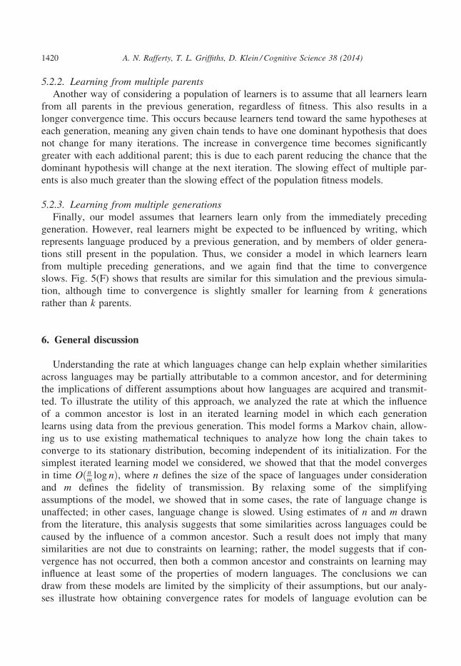
5.2.2. Learning from multiple parentsAnother way of considering a population of learners is to assume that all learners learn

from all parents in the previous generation, regardless of fitness. This also results in a

longer convergence time. This occurs because learners tend toward the same hypotheses at

each generation, meaning any given chain tends to have one dominant hypothesis that does

not change for many iterations. The increase in convergence time becomes significantly

greater with each additional parent; this is due to each parent reducing the chance that the

dominant hypothesis will change at the next iteration. The slowing effect of multiple par-

ents is also much greater than the slowing effect of the population fitness models.

5.2.3. Learning from multiple generationsFinally, our model assumes that learners learn only from the immediately preceding

generation. However, real learners might be expected to be influenced by writing, which

represents language produced by a previous generation, and by members of older genera-

tions still present in the population. Thus, we consider a model in which learners learn

from multiple preceding generations, and we again find that the time to convergence

slows. Fig. 5(F) shows that results are similar for this simulation and the previous simula-

tion, although time to convergence is slightly smaller for learning from k generations

rather than k parents.

6. General discussion

Understanding the rate at which languages change can help explain whether similarities

across languages may be partially attributable to a common ancestor, and for determining

the implications of different assumptions about how languages are acquired and transmit-

ted. To illustrate the utility of this approach, we analyzed the rate at which the influence

of a common ancestor is lost in an iterated learning model in which each generation

learns using data from the previous generation. This model forms a Markov chain, allow-

ing us to use existing mathematical techniques to analyze how long the chain takes to

converge to its stationary distribution, becoming independent of its initialization. For the

simplest iterated learning model we considered, we showed that that the model converges

in time Oðnm log nÞ, where n defines the size of the space of languages under consideration

and m defines the fidelity of transmission. By relaxing some of the simplifying

assumptions of the model, we showed that in some cases, the rate of language change is

unaffected; in other cases, language change is slowed. Using estimates of n and m drawn

from the literature, this analysis suggests that some similarities across languages could be

caused by the influence of a common ancestor. Such a result does not imply that many

similarities are not due to constraints on learning; rather, the model suggests that if con-

vergence has not occurred, then both a common ancestor and constraints on learning may

influence at least some of the properties of modern languages. The conclusions we can

draw from these models are limited by the simplicity of their assumptions, but our analy-

ses illustrate how obtaining convergence rates for models of language evolution can be


used to draw conclusions about the origins of similarities across languages, paving the

way for the investigation of these questions using more realistic models.

In the remainder of the paper, we situate the models we have used within the broader

literature, consider the limitations of our analysis, and highlight some directions for future

work.

6.1. Relation to other models

We analyzed the rate of convergence of models of language evolution in order to under-

stand how quickly the influence of a common ancestor is lost. Niyogi (2006) have consid-

ered this question for several other language learning algorithms. There also exist a variety

of other approaches that can assist in answering this question. One such approach is the

reconstruction of earlier languages based on their descendant languages. Such approaches

often additionally examine how quickly the descendant languages diverged (Evans, Ringe,

& Warnow, 2004; Swadesh, 1952). While these efforts remains controversial, the fact that

they are even partially successful suggests that at least some evidence of the common

ancestor can be traced back for a significant period. As mentioned at the beginning of this

paper, reconstruction work has also found that current patterns across languages can be

used to recapture some information about a common ancestral language (Dunn et al.,

2011; Gell-Mann & Ruhlen, 2011). Again, this supports the claim that there are similarities

across languages that are not solely caused by biases in human learning or innate linguistic

universals. We see our results as a complement to this existing work that can help to clarify

how modifications to a model of language evolution can affect time to convergence.

6.2. Limitations of the analysis

We have already discussed some of the challenges posed by connecting our mathemat-

ical results to real processes of language change and considered some of the ways in

which our models can be modified to be more realistic. In this section, we consider some

of the more technical limitations of our analysis. For the mathematical analysis of conver-

gence rate, we gave asymptotic bounds, which ignore proportionality constants. Such con-

stants are independent of the relationship between the space of possible languages and

the rate at which errors in learning occur (as defined by n and m) but can have practical

implications for applying the bound to understanding the rate of language change in the

world. In the case of the bound we showed for the Principles and Parameters model, this

proportionality constant is known; this fact was used to make Fig. 4 showing convergence

rates based on one’s beliefs about the values of n and m and to interpret the consequences

of plausible estimates of n and m drawn from the literature. For the extensions of the

model, the proportionality constants are not known, and in many cases, we have not pro-

vided explicit bounds. Instead, one must use simulation results to assess how quickly a

particular model of language change will converge. Establishing bounds with known con-

stants is a significant challenge, but one that we hope may ultimately be addressed

through advances in the mathematical analysis of Markov chains.


A second limitation of our analysis is that we have only considered language represen-

tations that result in a discrete and finite set of possible languages. By focusing on hypoth-

esis spaces based on Principles and Parameters and Optimality Theory, our analysis

assumes that languages that cannot be represented by these systems are unlearnable. This

is a strong assumption, and it necessarily dictates that certain linguistic universals are due

to constraints on human learning. One could relax this assumption by considering hypothe-

sis spaces with an infinite number of languages. However, our analyses relied on results

from the analysis of discrete Markov chains to assess the rate of convergence, and these

results do not necessarily generalize when we consider language representations that allow

infinite numbers of languages. In our formulation of the problem, converging to a station-

ary distribution is an instance of a random walk over a space of possible languages. It has

been shown that discrete random walks will always converge to a stationary distribution

given relatively simple technical conditions, while continuous random walks do not always

converge to a stationary distribution (Woess, 2000). Thus, it is possible that such an analy-

sis would predict that the influence of the common ancestor would never be completely

lost. The results of Griffiths and Kalish (2007) do generalize to continuous Markov chains,

indicating that we should expect models of language evolution based on iterated learning

with Bayesian learners to have stationary distributions. However, obtaining convergence

rates for these models remains a challenge, except in the simplest cases.

6.3. Future work

We view our work as a first step in understanding how different assumptions in models

of language evolution affect the rate at which the resulting languages lose the influence of

a common ancestor. There are many ways in which this work could be extended. We have

shown results for an arbitrary prior distribution. However, the structure of this distribution,

which reflects cognitive biases, might be restricted in ways that shorten time to conver-

gence. For example, if certain structures are unlearnable (as discussed in, e.g., Hunter,

Lidz, Wellwood, & Conroy, 2010; Pinker & Jackendoff, 2009), then the number of possi-

ble languages is effectively decreased, lowering time to convergence.

While we considered a variety of relaxations of our original assumptions about lan-

guage transmission, addressing what we saw as the most unrealistic assumptions, there

remain a variety of possible relaxations that we did not consider. The framework we have

presented allows one to consider how new variations might affect convergence time, and

given the similarity of results across different relaxations, we believe that most other

relaxations which bring the model closer to human language would also slow conver-

gence time. We have examined relatively few relaxations that incorporate communicative

pressures. There are a number of other ways of conceptualizing these pressures (e.g.,

Tily, 2010) that might lead to somewhat different results. Such pressures might decrease

the time for an improbable feature of the common ancestor to disappear, but they could

conversely increase the time for improbable but possible variants to be attested.

There are also influences on language change that do not fit as easily into the iterated

learning framework that we have presented. One such influence is geographic factors.


Languages that are spoken by neighboring groups are likely to influence one another. To

incorporate this factor into iterated learning, one might augment each learner with a loca-

tion and have multiple descendants from each parent, each of which may migrate to a

slightly different location. Learners may then learn both from their parent as well as from

those who are geographically close to them. Such a model is likely to have different con-

vergence properties than the iterated learning models we considered and would be a com-

bination of models of language learning and human migration.

Social factors, including deliberate language changes by social groups to differentiate

from one another (Labov, 2001), are also outside the scope of the analysis we have pre-

sented. While these factors clearly result in language change, it is less obvious how to

incorporate them into our mathematical model of language change and thus what effect

they have on convergence time. Are the changes a straightforward application of cogni-

tive biases, making them the equivalent of increasing m and thus decreasing convergence

time, or are the new languages derived from the old languages such that constraints on

learning are less relevant than in cases where the fidelity of transmission is limited? Due

to such complexities we did not incorporate social factors into our analyses, but this is

clearly a direction that deserves further investigation.

7. Conclusion

Answering questions about the history of modern languages is challenging. Computa-

tional models provide a set of tools that can be used to explore the implications that dif-

ferent assumptions about language evolution have for this history. In this paper, we have

shown how the question of whether the similarities between modern languages are par-

tially due to the influence of a common ancestor can be expressed mathematically in

terms of the convergence rates of stochastic processes that result from models of lan-

guage evolution. We have illustrated how this approach can be used, analyzing the impli-

cations of a simple model of how languages are learned and transmitted. This analysis

can be used to link theoretical and empirical results about language learning and language

change to answers about the origins of similarities across languages. Drawing stronger

conclusions will require analyzing more realistic models. We took a first step in this

direction by exploring the effects of changing the assumptions behind our model, showing

that these changes generally maintained the conclusions drawn from the original model.

We hope that the methodology we have adopted allows others to take further steps along

this path, ultimately yielding answers to some of the deep questions about the nature of

linguistic universals.

Acknowledgments

This work was supported by a National Science Foundation Graduate Fellowship and a

National Defense Science & Engineering Graduate Fellowship to Anna N. Rafferty and


by National Science Foundation grants IIS-1018733 to Dan Klein and Thomas L.

Griffiths and BCS-0704034 to Thomas L. Griffiths. Preliminary results from this work

were presented at the 31st Annual Conference of the Cognitive Science Society in 2009.

Notes

1. Note that each generation may consist of a single learner or of a population of

learners. Similar analytic results apply in both cases (Griffiths & Kalish, 2007); we

primarily consider the case of a single learner at each generation.

2. Throughout this paper, we assume a finite space of possible languages in order to

make computation tractable. In the Discussion, we consider possible implications

of an unbounded space of languages.

3. Note that these various probabilities form our model of the learners. Learners need

not actually hold them explicitly, nor perform the exact computations, provided that

they act as if they do.

4. An intuition for this result comes from the following argument. A sufficient condi-

tion for convergence to the uniform prior we have assumed is that all parameters

have been left unspecified in the data at least once. This is true because each time

a parameter is left undefined, its new value is insensitive to its current value. The

result after all parameters have been left unspecified at least once is then equivalent

to drawing a vector of values uniformly at random. The time to convergence is thus

upper-bounded by the time required to sample all parameters at least once. This is

a version of the coupon-collector problem, being equivalent to asking how many

boxes of cereal one must purchase to collect n distinct coupons, assuming each box

contains one of the n coupons and coupons are distributed uniformly over boxes

(Feller, 1968). The first box provides one coupon, but then the chance of getting a

distinct coupon in the next box is (n � 1)/n. In general, the chance of getting a dis-

tinct coupon in the next box after obtaining a total of i different coupons is

(n � i)/n. The expected time to find the next coupon is thus n/(n � i), and the

expected time to find all coupons is nPn

i¼11i, or n times the nth harmonic number.

The bound of n log n results from an asymptotic analysis of the harmonic numbers,

showing that the largest term in the asymptotic approximation grows as log n as nbecomes large.

5. Since a parameter may be dropped but take a new value that is the same as the

previous one, the expected number of parameters to actually change per generation

is upper bounded by rather than equal to the value of m.6. Intuitively, this rate can again be interpreted using the coupon-collector problem.

At every step, the learner changes unknown parameters to match the prototype.

The problem is thus still analogous to the coupon-collector problem, with the worst

case being when all n parameters differ from the prototype.


References

Atkinson, Q. (2011). Phonemic diversity supports a serial founder effect model of language expansion from

Africa. Science, 332(6027), 346.Bengtson, J. D., & Ruhlen, M. (1994). Global etymologies. In M. Ruhlen (Ed.), On the origin of languages:

Studies in linguistic taxonomy (pp. 277–336). Stanford, CA: Stanford University Press.

Chomsky, N. (1965). Aspects of the theory of syntax. Cambridge, MA: MIT Press.

Chomsky, N., & Lasnik, H. (1993). The theory of principles and parameters. In J. Jacobs, A. von Stechow,

W. Sternefeld, & T. Vannemann ( Eds.), Syntax: An international handbook of contemporary research(pp. 506–569). Berlin: Walter de Gruyter.

Comrie, B. (1981). Language universals and linguistic typology. Chicago: University of Chicago Press.

Diaconis, P., & Saloff-Coste, L. (1993). Comparison techniques for random walk on finite groups. TheAnnals of Probability, 21(4), 2131–2156.

Diaconis, P., & Saloff-Coste, L. (1996). Random walks on finite groups: A survey of analytic techniques. In

H. Heyer (Ed.), Probability measures on groups and related structures Vol. XI (44–75). Singapore: World

Scientific.

Dunn, M., Greenhill, S. J., Levinson, S. C., & Gray, R. D. (2011). Evolved structure of language shows

lineage-specific trends in word-order universals. Nature, 473(7345), 79–82.Evans, S., Ringe, D., & Warnow, T. (2006). Inference of divergence times as a statistical inverse problem. In

P. Forster & C. Renfrew (Eds.), Phylogenetic methods and the prehistory of languages, (pp. 119–130).McDonald Institute for Archaeological Research.

Feller, W. (1968). An introduction to probability theory and its applications. New York: Wiley.

Gell-Mann, M., & Ruhlen, M. (2011). The origin and evolution of word order. Proceedings of the NationalAcademy of Sciences, 108(42), 17290–17295.

Gibson, E., & Wexler, K. (1994). Triggers. Linguistic Inquiry, 25, 355–407.Greenberg, J. H. (Ed.). (1963). Universals of language. Cambridge, MA: MIT Press.

Greenberg, J. H. (2002). Indo-European and its closest relatives: The Eurasiatic language family. Stanford,CA: Stanford University Press.

Griffiths, T. L., & Kalish, M. L. (2007). A Bayesian view of language evolution by iterated learning.

Cognitive Science, 31, 441–480.Hawkins, J. (Ed.). (1988). Explaining language universals. Oxford, UK: Blackwell.Holden, C. (1998). No last word on language origins. Science, 282(5393), 1455.Hroarsdottir, T. (2000). Word order change in Icelandic: From OV to VO. Amsterdam: John Benjamins

Publishing Company.

Hunter, T., Lidz, J., Wellwood, A., & Conroy, A. (2010). Restrictions on the meaning of determiners: Typological

generalisations and learnability. In E. Cormany, S. Ito, & D Lutz ( Eds.), Proceedings of SALT Vol. 19(pp. 223–238).

Kayne, R. S. (2000). Parameters and universals. New York: Oxford University Press.

Kirby, S. (2001). Spontaneous evolution of linguistic structure: An iterated learning model of the emergence

of regularity and irregularity. IEEE Journal of Evolutionary Computation, 5, 102–110.Kirby, S., Smith, K., & Brighton, H. (2004). From UG to universals: Linguistic adaptation through iterated

learning. Studies in Language, 28, 587–607.Kirby, S., Dowman, M., & Griffiths, T. L. (2007). Innateness and culture in the evolution of language.

Proceedings of the National Academy of Sciences, 104, 5241–5245.Komarova, N. L., & Nowak, M. A. (2003). Language dynamics in finite populations. Journal of Theoretical

Biology, 221(3), 445–457.Krupa, V. (1982). Syntactic typology and linearization. Language, 58(3), 639–645.Labov, W. (2001). Principles of linguistic change. Volume II: Social factors. Oxford, UK: Wiley-Blackwell.


Levin, D. A., Peres, Y., & Wilmer, E. L. (2009). Markov chains and mixing times. American MathematicalSociety, Providence, RI.

Lightfoot, D. (1999). The development of language: Acquisition, change and evolution. Oxford, UK: Blackwell.McCarthy, J. J. (2004). Optimality theory in phonology: A reader. Malden, MA: Wiley-Blackwell.

Niyogi, P. (2006). The computational nature of language learning and evolution. Cambridge, MA: MIT Press.

Niyogi, P., & Berwick, R. C. (1996). A language learning model for finite parameter spaces. Cognition, 61,161–193.

Norris, J. R. (1997). Markov chains. Cambridge, UK: Cambridge University Press.

Picard, M. (1998Evidence from Algonquian. International Journal of American Linguistics, 64(2), 141–147.Pinker, S., & Jackendoff, R. (2009). The reality of a universal language faculty. Behavioral and Brain

Sciences, 32(05), 465–466.Prince, A., & Smolensky, P. (2004). Optimality theory: Constraint interaction in generative grammar.

Oxford, UK: Blackwell.

Smith, K., Kirby, S., & Brighton, H. (2003). Iterated learning: A framework for the emergence of language.

Artificial Life, 9, 371–386.Swadesh, M. (1952). Lexico-statistic dating of prehistoric ethnic contacts: With special reference to north

american indians and eskimos. Proceedings of the American Philosophical Society, 96(4), 452–463.Taylor, A. (1994). The change from SOV to SVO in Ancient Greek. Language variation and change, 6(01),

1–37.Tily, H. (2010). The role of processing complexity in word order variation and change. Unpublished doctoral

dissertation, Stanford University.

Tily, H., Frank, M., & Jaeger, T. (2011). The learnability of constructed languages reflects typological

patterns. In L. Carlson, C. Hoelscher, & T. F. Shipley (Eds.), Proceedings of the 33rd Annual Conferenceof the Cognitive Science Society (pp. 1364–1369). Austin, TX: Cognitive Science Society.

Woess, W. (2000). Random walks on infinite graphs and groups Vol. 138. Cambridge, UK: Cambridge

University Press.

Appendix A: Relaxing model assumptions

We provide additional information below concerning the technical details of simula-

tions. Additionally, Fig. 5 in the main text shows the results of simulations for each mod-

ification to the basic model.

A.1. Optimality Theory

To specify a Bayesian learner that uses a representation inspired by Optimality Theory

(OT), we must identify the hypothesis space H, data space D, prior p(h), and likelihood

p(d|h). In this representation, each hypothesis is an ordered list of n constraints, with the

order of constraints representing rank. The hypothesis space H is thus the symmetric

group of permutations of rank n, Sn and is of size n!. We assume learners see sufficient

data to specify the relative ordering of all but m constraints. The data space is then

strings over {1, 2,. . .n} of length n � m, with no repeated elements, ordered from left-to-

right in order of precedence (see Fig. A1). The relative ordering of the n�m specified

constraints is maintained exactly from the generating hypothesis. We again see that the


likelihood, p(d|h), is 0 for all orderings not consistent with our hypothesis and equal for

all consistent orderings. Analogously to the previous case, we select m constraints to

remove from the ranking randomly, givingnm

� �possible data strings for each hypothe-

sis. This gives pðdjhÞ ¼ m!ðn�mÞ!n! . Thus, the posterior is the same as for the Principles and

Parameters representation. Since we can freely permute m of our parameters, we haven!

ðn�mÞ! consistent hypotheses for any data string d. If our prior is uniform, then

pðhjdÞ ¼ ðn�mÞ!n! for all consistent h and 0 otherwise.

To bound the convergence of iterated learning with an Optimality Theory representa-

tion, we assume that, at each generation, the learner has sufficient data to rank all but mof n constraints. First consider the case where m = 1. The process of changing the order-

ing of one item in a permutation while leaving the relative ordering of the other items

unchanged has been studied previously in the context of a random-to-random shuffle (see

Fig. A1). The best bound for the random-to-random shuffle is O(n log n) by Diaconis

and Saloff-Coste (1993), with the intuitive argument being similar to that given for the

Principles and Parameters convergence bound. As before, we view each iteration as msuccessive steps, making time to convergence Oðnm log nÞ.

A.2. Non-uniform priors

We consider the case of learners who have a non-uniform prior over the languages in

the hypothesis space. The uniform prior is the unique maximum entropy distribution for

any hypothesis space. However, there is no unique solution for achieving a given entropy

for a distribution with k values. Thus, we altered entropy in the following, non-unique

way. We define one hypothesis hp as the prototypical hypothesis. Then, we calculate the

distance between hp and h for each hypothesis h using the Hamming distance D. Then,

C(A) (B)

Remove card

Reinsert

BA

CA

CAB

ABC

AC

ABCB

AC A

CB

ht-1 dt-1 ht

Fig. A1. Assumptions for model inspired by Optimality Theory (OT). (A) Representation of a hypothesis

and data item for OT. The relative ordering of A and C is preserved in the data, but not the ordering of B.(B) Movement among hypotheses for the OT case is analogous to a shuffle in which a random card (in this

case, the gray card) is removed and reinserted into a random spot.


for all h, p(h)/ exp (�bD(h,hp)). Changing b changes the entropy of the distribution.

Changing entropy in this manner gives our priors a characteristic shape: hp has maximum

probability, and the probability of other hypotheses decreases with distance from hp. Foran evenly spaced range of b (from 0 to 6 in increments of 0.05), we calculated the time

to convergence when the resulting prior was used, fixing n = 6 and m = 2. As the

entropy of the prior decreases, the time to convergence increases, as mentioned in the

main text. This result differs from previous simulations reported in earlier work because

it is worst-case time bound rather than an expected time bound.

A.3. Choosing a hypothesis from the posterior

In the main article, we note that exponentiated sampling from a non-uniform distribu-

tion is equivalent to using a prior that has been transformed. In particular, raising the pos-

terior to the power of c before sampling is equivalent to multiplying the b parameter in

the model we used to construct our non-uniform priors by c.

A.4. Non-uniform parameter dropping

To model the situation in which certain parameters are more likely to be dropped at

each iteration than others, we put a non-uniform distribution over the probability that any

particular parameter will be dropped conditioned on the total number of parameters to

drop. We consider the parameter in each place i = 1,. . .,n, and define the probability of

dropping the ith parameter given m as proportional to exp (�a(i � 1)). Assuming that

the probability of dropping each parameter is independent of the others given this condi-

tioning (e.g., dropping the first parameter does not make dropping the second parameter

more or less likely), then we can calculate the probability of a particular hypothesis given

m asQn

i¼1 pðdiÞIðdi¼?Þð1 � pðdiÞ1�Iðdi¼?ÞÞ. With this definition, we can calculate transitions

exactly, as in previous simulations. Time to convergence increases as the entropy of the

distribution over dropping parameters decreases.

A.5. Modifications to population structure

We consider several ways that an iterated learning model might incorporate interaction

between multiple learners in order to see how this change affects convergence time. The

additional complexity of these models means that we cannot calculate the total variation

distance exactly. Instead, we use an empirical approximation of total variation distance,

described below.

Quantitatively, we analyze convergence for the following simulations by computing an

empirical total variation distance. For each simulation, we run many parallel chains, all

with the same starting point. We choose the starting point likely to cause the slowest con-

vergence by starting all learners in the same language in those cases where there are mul-

tiple learners per generation. We then average the language distributions across chains at

each iteration, giving an average language distribution for each iteration of the simula-


tion. The total variation distance between this distribution and the prior can then be cal-

culated. While the stationary distributions for these simulations may not be equal to the

prior distribution in the general case, by symmetry the prior is the stationary distribution

in the uniform case. Thus, we are able to calculate the total variation distance between

the language distribution at each iteration and the stationary distribution.

This empirical total variation distance raises another issue, however, due to the fact

that we have a finite sample. Even if samples were drawn directly from the prior distri-

bution, the total variation distance between a distribution over those samples and the

prior distribution would be non-zero. To handle this issue, we developed the following

empirical convergence criterion. We would like to find a cutoff point for the total varia-

tion distance such that when we reach this cutoff, we have converged. Given a simula-

tion to be checked for convergence, samples are drawn from the stationary distribution at

each iteration. The number of samples drawn per iteration is equal to the number of sim-

ulated chains. Then, after drawing all samples for all iterations, we can again average

our distributions and calculate total variation distance. To ensure convergence, we choose

a cutoff value such that for 95% of iterations based on draws from the prior, the total

variation distance is less than the cutoff. By choosing such a cutoff value and starting all

learners at the “worst” point for convergence, we find an upper bound for time to con-

vergence.

There is one remaining issue: All of the simulations below involve multiple learners

per generation, but the hypotheses of the learners are likely to be highly correlated. Thus,

it would not be correct to sample the distribution as a collection of independent draws

from the prior: Doing so would make many simulations fail to converge by this empirical

criterion even after they have clearly converged by other measures. We thus treat the

multiple correlated learners as equivalent to one learner. Consequently, we draw a sample

for only one learner per iteration per simulated chain.

A.6. Population fitness model

In the main paper, we consider a population fitness model in which multiple learners

exist at each generation. Each learner has a single parent from whom language is learned,

and parents are sampled based on the their fitness. Fitness is a measure of the communi-

cative efficacy of a speaker based on the languages spoken by those in the population.

For each generation, we define the fitness of learner i as fi ¼Pn

j¼1 pðparameterjÞ, wherep(parameterj) is the proportion of the population with the same value for parameter j asspeaker fi. For example, if we have three learners speaking languages 1,010, 1,000, and

0,010, the first will have f1 ¼ 23þ 1 þ 2

3þ 1 ¼ 10

3, while the other two will have

f2 ¼ f3 ¼ 23þ 1 þ 1

3þ 1 ¼ 3. We call this the additive function for population fitness.

We also consider a multiplicative function for population fitness. In this case,

fi ¼Qn

j¼1 pðparameterjÞ. Intuitively, the multiplication function penalizes learners more

strongly for having a parameter value that differs from the norm. In the additive example,

the first learner has only slightly higher fitness than the other two. Using the multiplica-


tive function, the first learner would have f1 ¼ 49while for the other two, f2 ¼ f3 ¼ 2

9.

Since the probability of learning from parent i is proportional to fi, this means that for

the additive function subsequent learners would be 109times as likely to choose parent 1

as to choose parent 2 or parent 3, while with the multiplicative function the learners

would be twice as likely to choose parent 1. Iterated learning then proceeds as in the ori-

ginal case except that each learner in a generation may be learning from a different par-

ent.

For this simulation and the following two simulations, the qualitative behavior of the

simulations is affected by the expected rate of parameter change (m). Asymptotically, Ko-

marova and Nowak (2003) show that assuming the noise level in learning is not too high,

learners will converge to a single language with high probability. In our case, this is

equivalent to saying that if m is not too high for our population fitness chain, as com-

pared to n, then learners will show linguistic coherence. This simply means that after suf-

ficient iterations have passed, members of the same generation in later iterations will

share the same language as one another.

For each fitness function, multiplicative and additive, we simulated how the time to

convergence was affected by the number of learners at each generation (ranging from 2

to 20). All simulations used n = 5 and m = 1. The empirical total variation distance was

calculated by determining the distribution over languages at each generation averaged

across 1,000 chains, as described above. The worst case starting point for these simula-

tions is to set all learners at the initial generation to have the same language, although

any particular language can be chosen due to symmetry.

Both population fitness simulations have some slowing effect on time to convergence

as the number of learners increases. However, this effect is extremely small when using

the additive function: when the number of learners is increased from 2 to 20, on average

only eight more iterations are required for convergence. We see a much stronger effect

for the multiplicative function, and the effect in this case appears to be exponential. The

reason for the slowing is that the dominant language in one generation is closely coupled

with the dominant language in the next generation. This coupling is more extreme when

the multiplicative fitness function is used. Qualitatively, we found that the dominant lan-

guage of the population stays the same over long periods. Thus, the Markov chain for this

simulation is slower to converge due to the tendency to remain at a language favored by

the starting point.

A.7. Learning from multiple parents

Another way of considering a population of learners is to assume that all learners learn

from all parents in the previous generation, regardless of fitness. This requires defining a

likelihood p(d|h), where d is a collection of ‘ data vectors, one from each parent. To

account for the fact that different parents may be producing data from different hypothe-

ses, leading to the possibility of data with conflicting settings for a single parameter, we

add a noise parameter e to our model. We can then calculate p(d|h) as:


pðhjdÞ ¼Y‘i¼1

pðhjdiÞ ð3Þ

/Y‘i¼1

pðdijhÞpðhÞ ð4Þ

/Y‘i¼1

Ynj¼1

�Iðhj 6¼dij;dij 6¼?Þð1� �ÞIðhj¼dijÞ ð5Þ

where I(�) takes the value 1 when its argument is true and 0 otherwise and dij is the jthparameter of data vector i. With this definition of p(d|h), we can simulate iterated learn-

ing steps as in the original case.

We varied the number of learners per generation, as well as e, to determine the effect

on time to convergence. For all simulations, we set n = 5 and m = 1, and calculated the

empirical total variation distance using 1,000 chains per simulation. As in the population

fitness case, we used the worst-case starting point in which all members of the initial gen-

eration share the same language. Simulation results showed that learning from multiple

parents increases time to convergence and as e decreases, time to convergence increases

further.

A.8. Learning from multiple generations

The technical details of the model for learning from multiple generations closely fol-

low the details of the model for learning from multiple parents. We tested how varying

the number of generations from which each learner learned as well as adjusting the noise

parameter e affected the time to convergence. Fixing n = 5 and m = 1, we ran 1,000

chains per simulation to calculate the empirical total variation distance. The chains began

with all previous generations sharing the same language, as this is the worst-case starting

point. Learning from multiple generations also slows convergence.


Documents

Analyzing the Rate at Which Languages Lose the Inﬂuence of