Scholars' Mine Scholars' Mine

Masters Theses Student Theses and Dissertations

Summer 2018

Analyzing large scale trajectory data to identify users with similar Analyzing large scale trajectory data to identify users with similar

behavior behavior

Tyler Clark Percy

Follow this and additional works at: https://scholarsmine.mst.edu/masters_theses

Part of the Computer Sciences Commons

Department: Department:

Recommended Citation Recommended Citation Percy, Tyler Clark, "Analyzing large scale trajectory data to identify users with similar behavior" (2018). Masters Theses. 7807. https://scholarsmine.mst.edu/masters_theses/7807

This thesis is brought to you by Scholars' Mine, a service of the Missouri S&T Library and Learning Resources. This work is protected by U. S. Copyright Law. Unauthorized use including reproduction for redistribution requires the permission of the copyright holder. For more information, please contact scholarsmine@mst.edu.

ANALYZING LARGE SCALE TRAJECTORY DATA TO IDENTIFY USERS WITH

SIMILAR BEHAVIOR

by

TYLER CLARK PERCY

A THESIS

Presented to the Faculty of the Graduate School of the

MISSOURI UNIVERSITY OF SCIENCE AND TECHNOLOGY

In Partial Fulfillment of the Requirements for the Degree

MASTER OF SCIENCE IN COMPUTER SCIENCE

2018

Approved by

Dan Lin, Advisor

Wei Jiang

Yanjie Fu

iii

ABSTRACT

In today’s society, social networks are a popular way to connect with friends and

family and share what’s going on in your life. With the Internet connecting us all closer

than ever before, it is increasingly common to use social networks to meet new friends

online that share similar interests instead of only connecting with those you already

know. For the problem of attempting to connect people with similar interests, this paper

proposes the foundation for a Geo-social network that aims to extract the semantic

meaning from users’ location history and use this information to find the similarity

between users. Once the similarity scores are obtained, the results are examined to extract

the groups of similar users for the Geo-social network. Computing similarity for a large

number of users and then grouping based on the results is a computationally intensive

task, but fortunately Apache Spark can be leveraged to execute the comparison and

clustering of users in parallel across multiple computers, increasing the computation

speed when compared to a centralized version and working quickly enough to suggest

friends in real time for a given user.

iv

ACKNOWLEDGMENTS

I would like to first thank my advisor, Dr. Dan Lin, for moving my journey as a

student forward immensely by getting me involved in research, informing me of the SFS

program, and helping me out lots along the way. I would also like to thank the SFS

program for providing the funding to continue my education as well as helping connect

me with great employers and peers.

I would also like to thank Wei Jiang and Yanjie Fu for being a part of my

committee as well as being great teachers in the classroom. Dr. Fu was the first person to

really spark my interest in data analysis and Dr. Jiang helped teach me about a whole new

field in privacy preserving protocols as well as concepts in distributed operating systems

that Spark takes advantage of.

Finally, I would like to thank my family and friends at Missouri S&T for helping

me throughout my time here.

v

TABLE OF CONTENTS

Page

ABSTRACT ....................................................................................................................... iii

ACKNOWLEDGMENTS ................................................................................................. iv

LIST OF ILLUSTRATIONS ............................................................................................ vii

NOMENCLATURE ........................................................................................................ viii

SECTION

1. INTRODUCTION ...................................................................................................... 1

1.1. BACKGROUND ................................................................................................ 1

1.2. RELATED WORK ............................................................................................. 2

1.3. PROBLEM DEFINITION .................................................................................. 2

2. SEMANTIC TRAVEL MATCHING ........................................................................ 5

2.1. MAXIMUM TRAVEL MATCHING................................................................. 5

2.2. SEMANTIC TRAVEL MATCHING ................................................................. 6

2.3. SEMANTIC TRAVEL MATCHING EXAMPLE ............................................. 8

2.4. ISSUE OF LOOPING LOCATIONS ................................................................. 9

3. MAXIMAL CLIQUE FINDING ............................................................................. 11

3.1. BRON-KERBOSCH ALGORITHM ................................................................ 11

3.2. BRON-KERBOSCH EXAMPLE ..................................................................... 13

3.3. PROGRAM SPECIFIC IMPLEMENTATION DETAILS .............................. 15

4. EXPERIMENT AND RESULTS ............................................................................. 16

4.1. EXPERIMENTAL DESIGN ............................................................................ 16

vi

4.2. GRAPH GENERATION .................................................................................. 17

4.3. TESTING RESULTS........................................................................................ 17

4.3.1. Similarity Comparison Results. .............................................................. 18

4.3.2. Clique Finding Results............................................................................18

4.3.3. Single User Addition. ............................................................................. 20

5. CONCLUSIONS ...................................................................................................... 24

5.1. FUTURE WORK .............................................................................................. 24

5.2. FINAL THOUGHTS ........................................................................................ 25

BIBLIOGRAPHY ............................................................................................................. 27

VITA .................................................................................................................................28

vii

LIST OF ILLUSTRATIONS

Figure Page

1.1. Two Different Trajectories ......................................................................................... 3

1.2. Example Three Clique Graph ..................................................................................... 4

2.1. Sample Location Hierarchy Tree ................................................................................ 7

2.2. Looping Location Trajectory .................................................................................... 10

3.1. Example Graph for Bron-Kerbosch Algorithm ........................................................ 14

3.2. Complete Process Overview ..................................................................................... 15

4.1. Full Similarity Comparison....................................................................................... 19

4.2. Comparing Spark with Centralized for Clique Finding ............................................ 20

4.3. Single User Clique Finding Results .......................................................................... 21

4.4. Single User Similarity Results .................................................................................. 22

4.5. Full Process Single User Addition ............................................................................ 23

viii

NOMENCLATURE

Symbol Description

t Threshold for Maximum Time Between Two Locations

Threshold for Minimum Similarity Between Two Users

φ Time Passed Between Two Trajectories

1. INTRODUCTION

1.1. BACKGROUND

Today, mobile devices with Internet are extremely common and almost all users

of these devices utilize some form of location-based service at some point, such as using

Google Maps to find nearby restaurants, getting directions from your current location or

checking in on Facebook or any other social network. Along with these devices being so

frequently used, more people are using GPS devices to record their location trajectories.

All of this means that there is more data than ever to take advantage of and analyze. By

looking at this large amount of trajectory data, it is possible to look at two different users

GPS trajectory data in order to determine if two users would be compatible.

However, people in various locations will never come up as similar if their GPS

data alone is considered. By looking at the locations in the real world it is possible to

extract some semantic meaning of the places visited by the user. When the semantic

meaning is obtained it is possible to identify users that have an overlap in interests, even

if their actual geographic location does not overlap [1][2]. By giving a similarity score

based on this semantic overlap, users can be clustered into groups that will identify

similar social groups. These social groups can then be used to match similar users

together for the Geo-Social network.

For this to be feasible, a similarity comparison between two trajectories that runs

within a reasonable amount of time is needed. After retrieving the similarity score for all

of the users in the dataset, a graph where users are connected if their similarity score is

above a threshold can be created. By examining this graph, it is possible find groups of

users that are connected to identify users who will most likely be compatible. By using

2

Spark, we can find the similarities between all users, which is a very computationally

heavy task for a centralized approach. Afterwards, Spark is also used to identify the

groups within the user dataset. To ensure that the groups contain users who are all very

similar, the approach to be used will find maximal cliques in the graph. This means that

all users in the group will be similar to every other user in the clique.

1.2. RELATED WORK

Two works [1] and [2], performed work that the similarity comparison used in

this paper draws inspiration from, finding similar user based on location history. The

objective of [1] is to estimate similarity between two users using the semantic meaning of

the location data. [2] Looks to mine user similarity based on the GPS trajectories taken

from the real world. The work from each of these papers lend themselves nicely to being

used for creating a geo-social network and the approach in this paper is similar for the

similarity comparison stage. One disadvantage to the method used in [2] that is addressed

in this paper, is the problem of looping locations within the users' location history. The

Bron & Kerbosch algorithm originally presented in [3], as well as improvements on the

algorithm presented in [4] are used for finding all maximal cliques within the graph of

users.

1.3. PROBLEM DEFINITION

The main goal of this work is to give a similarity score to the trajectory data of

two different users and use the results to identify all cliques within the graph of users to

3

set the stage for creation of a geo-social network. Before continuing, there are some terms

that will be used frequently and are important to know in order to understand the

approach.

A trajectory is a sequence of locations with information about the time spent at

each location and the time it takes to travel between locations in the sequence. Below is

an example of a trajectory.

𝑇𝑟𝑎𝑗 = 𝑝1, 𝑝2, 𝑝3, … 𝑝𝑛: 𝑤ℎ𝑒𝑟𝑒 𝑝𝑖 = (𝑙𝑜𝑐𝑎𝑡𝑖𝑜𝑛 𝑛𝑎𝑚𝑒, 𝑠𝑡𝑎𝑦 𝑡𝑖𝑚𝑒, 𝑡𝑟𝑎𝑣𝑒𝑙 𝑡𝑖𝑚𝑒) (1)

Trajectories tell a lot about the users who submit them and are vital to the

algorithm. Therefore, it is important to get a firm grasp on the idea of what a trajectory is

and how it is visualized other works. Below, Figure 1.1 shows an example of some made

up trajectories to be compared. By looking at these two trajectories and using our

algorithm we can give a score that will give an idea of how similar the two trajectories

are.

Figure 1.1. Two Different Trajectories

4

After finding the similarity score between all users, a graph will be constructed

where the graphs vertices represent users, and an edge between nodes indicates a

similarity over the chosen threshold, α. The approach that is used in this paper focuses on

grouping the users by finding the cliques in the graph. A clique is a subset of vertices, all

adjacent to each other, within a graph. Figure 1.2. below shows an example graph with 3

cliques.

Figure 1.2. Example Three Clique Graph

5

2. SEMANTIC TRAVEL MATCHING

2.1. MAXIMUM TRAVEL MATCHING

The approach used in [1] involves finding and measuring the length of the

maximal travel matches found when comparing two user’s trajectories. A regular travel

match between two sub-sequences is found when a given constant maximum time

difference between stay times, 𝑡, and two sub-sequences of trajectories 𝑇1(𝑎1, 𝑎2, … 𝑎𝑛)

and 𝑇2(𝑏1, 𝑏2, … 𝑏𝑛) meet the following conditions

1. ∀ 𝑖 𝜖 [1, 𝑘]: 𝑎𝑖 = 𝑏𝑖

2. ∀ 𝑖 𝜖 [2, 𝑘]: 𝑇ℎ𝑒 𝑡𝑟𝑎𝑣𝑒𝑙 𝑡𝑖𝑚𝑒 𝑏𝑒𝑡𝑤𝑒𝑒𝑛 𝑡𝑤𝑜 𝑙𝑜𝑐𝑎𝑡𝑖𝑜𝑛𝑠 𝑎𝑖 𝑎𝑛𝑑 𝑎𝑖+1 𝑎𝑛𝑑

𝑏𝑖 𝑎𝑛𝑑 𝑏𝑖+1 𝑖𝑠 𝑙𝑒𝑠𝑠 𝑡ℎ𝑎𝑛 𝑡ℎ𝑒 𝑚𝑎𝑥𝑖𝑚𝑢𝑚 𝑡𝑖𝑚𝑒 𝑑𝑖𝑓𝑓𝑒𝑟𝑒𝑛𝑐𝑒 𝑐𝑜𝑛𝑠𝑡𝑎𝑛𝑡 𝑡.

Furthermore, a travel match is maximal if it has no more locations that match

within the time constraint to be added on to the start, somewhere in the middle, or the end

of the travel match.

Finding the maximum travel match between two sequences tells a lot about how

similar they are. If two people have a long match in things that they do throughout the

day and how long they do these things, it is very likely that they share similar interests or

at the very least a similar lifestyle. One important thing to note is that using the maximum

travel match to compute the similarity score causes the score to have no upper bound,

even if two trajectories are matching exactly, they could always be matching with one

more location added.

6

2.2. SEMANTIC TRAVEL MATCHING

As discussed previously, the goal is of the algorithm is to be able to compare

location trajectories that do not share any geographic overlap. Simply checking if the

names of the locations match may not suffice for finding an actual match. For example, if

two people are both college students at different schools that spend 10 hours and school

then return immediately home every day, simply comparing the value of Missouri S&T to

Mizzou or their GPS values would not indicate a match, although for all intents and

purposes, these two locations are semantically similar, and certainly indicate a level of

similarity just below an exact match. To address this problem, a tree to represent a

semantic location hierarchy will be constructed that can be referenced when comparing

two different trajectories. The lower level you go on the tree, the closer the semantic

meaning of the locations and as you climb the tree the descriptions become more general.

For example, Taco Bell and McDonalds would both be at the same level of the

tree under a node named Fast Food Restaurants which might be under an even more

general category labeled Food. Creating a tree that had all possible values we would need

would take an extremely long time and would be a whole research project on its own, so

for now a simple semantic hierarchy tree that demonstrates the effectiveness of this

approach will be used for the current implementation of the algorithm.

In the future a much more in-depth tree will be a requirement. One project has

already worked on creating a web that links together the English language together based

on the semantic similarity of words called WordNet [5]. The use of WordNet will

eventually replace the sample semantic hierarchy tree in the future when looking to scale

7

outward and accept even more types of location input data, but for the remainder of this

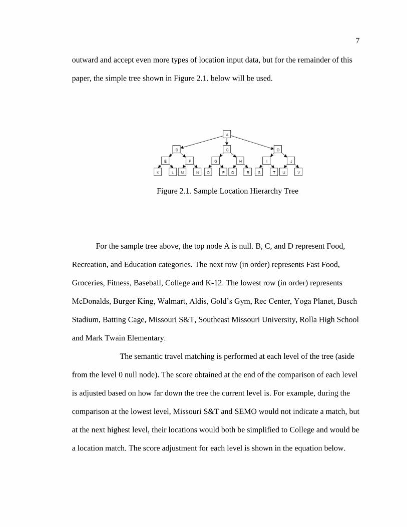
paper, the simple tree shown in Figure 2.1. below will be used.

Figure 2.1. Sample Location Hierarchy Tree

For the sample tree above, the top node A is null. B, C, and D represent Food,

Recreation, and Education categories. The next row (in order) represents Fast Food,

Groceries, Fitness, Baseball, College and K-12. The lowest row (in order) represents

McDonalds, Burger King, Walmart, Aldis, Gold’s Gym, Rec Center, Yoga Planet, Busch

Stadium, Batting Cage, Missouri S&T, Southeast Missouri University, Rolla High School

and Mark Twain Elementary.

The semantic travel matching is performed at each level of the tree (aside

from the level 0 null node). The score obtained at the end of the comparison of each level

is adjusted based on how far down the tree the current level is. For example, during the

comparison at the lowest level, Missouri S&T and SEMO would not indicate a match, but

at the next highest level, their locations would both be simplified to College and would be

a location match. The score adjustment for each level is shown in the equation below.

8

Adjusted Score = Score ∗ 2𝑙𝑒𝑣𝑒𝑙−1 (2)

To measure the similarity of two trajectories, there is a max allowable difference

in time t and a time passed for each trajectory, φ, which is initially 0. Then starting at the

initial location for each user, a check is done to see if the locations at the current are the

same. If they are, add to the matching score and move to the next location, adding stay

and travel time to each trajectories time passed. If the locations do not match, there are

two possible paths. The first is to compare the current location of the first trajectory with

the next location of the second trajectory, incrementing the second trajectory’s time

passed. The second is if the next location for the second user cannot be reached without

surpassing max difference in time. The check will move 𝑇2 to the last matching location

and increment 𝑇1 to the next location, increasing 𝑇1’s time. Once this process is over, the

algorithm moves up a level of the semantic hierarchy tree and repeats, this time adding

less points for each match than the lower level.

2.3. SEMANTIC TRAVEL MATCHING EXAMPLE

To demonstrate, a comparison between 𝑇1 and 𝑇2 , which are shown above as the

top and bottom trajectories respectively in Figure 1.1. above. The comparison will be run

with an initial matching score = 8 at level = 1, and max time difference of 2. First, the

algorithm compares Rec Center and Golds Gym and it is a match, and the score is

increased. The 𝑇1 time is equal to 1.5 and 𝑇2 to 2. Compare Burger King and

McDonald’s, which are not equal at the current level, so move 𝑇1 to next 𝑇2 location

9

with time of 3.25. Next, comparison between Burger King and SEMO not a match, so we

move to next 𝑇2 location, surpassing the given t. So now, 𝑇1 goes to MS&T with time

2.25 and 𝑇2 goes back to McDonalds with time 2. They are not a match so 𝑇2 goes to

SEMO with time 3.25. SEMO and MS&T do not match so move 𝑇2 to Aldi’s with time

11.25. The max time difference has been reached and now the algorithm moves back to

SEMO and move, 𝑇1 to Walmart with time 10.75. Max time difference has been reached

so move 𝑇2 to Aldi’s with time 11.25. Finally, compare to Walmart and it is not a match

so finish for this level, with score 8. Now the matching score is adjusted for the current

level, which keeps it at 8. If continued, the process would then be repeated moving up

one level one the semantic hierarchy tree. After each level is calculated the score for each

level is then combined as the final similarity score between the two users.

It can be seen how this approach would be computationally intensive and

impractical for a large amount of data with a centralized approach. That is where Spark

comes in. Multiple comparisons can be computed in parallel using a Spark DataFrame

with our trajectory comparison algorithm as a user defined function that is executed

between each pair of users at a given level in our dataset at the same time. In this way, it

is possible to not only spread out the comparison of users, but also each individual

hierarchy level between the nodes in the Spark cluster.

2.4. ISSUE OF LOOPING LOCATIONS

Throughout the day, it may be very common for users to visit the same location

multiple times. For example, the user leaves his home to go to school, then returns home

10

for lunch and heads back to school again until finally heading home for the day. The

similarity comparison algorithms given in [1] and [2] does not deal with this issue and

seeing as this would likely be a frequent scenario when analyzing the entire day of users,

the similarity comparison in this paper has been modified to be able to handle looping

locations. When constructing the adjacency matrix used to find the maximal length path,

each repeat location will have its own node in the graph instead of looping caused from

returning back up the tree. Figure 2.2. shows and example of a looping trajectory.

Figure 2.2. Looping Location Trajectory

11

3. MAXIMAL CLIQUE FINDING

3.1. BRON-KERBOSCH ALGORITHM

After computing the similarity between all users, the graph of users will be

constructed to leverage graph theory to find the cliques within the users. Each node in the

graph will indicate a user in the dataset, and an edge between two nodes will indicate a

similarity score over a certain threshold, α. Within this graph, the goal is to find all the

groups of users that are fully connected to each other, which indicates that their locations

throughout the day are semantically similar.

After first testing a naïve approach for clique finding, the Bron-Kerbosch

algorithm has proven to be the best method to use when finding all cliques within the user

similarity graph. This approach was chosen because, although it may have a higher

complexity than other clique finding algorithms, it is one of the best for finding all

maximal cliques in practice [4]. Another benefit of using the Bron-Kerbosch algorithm,

or any clique finding as our method for grouping similar users together, is that this type

of “clustering” does not require any cluster validation because it is already guaranteed

that every user in the clique is above the similarity threshold with all other users in the

group.

The Bron-Kerbosch algorithm is a simple backtracking procedure that works

recursively to solve sub problems using three sets of nodes. The three sets are called R, X,

and P. R contains the nodes that are required to be included in the partial clique. X

contains the nodes that are going to be excluded from the clique. P contains the nodes

that have not yet been considered. The algorithm finds maximal cliques that include all

the vertices in R, some of the vertices in P and none of the vertices in X. In each recursive

12

call to the algorithm, P and X are disjoint sets where the union contains the vertices that

form a clique when they are added to R. When P and X are both empty, there are no more

nodes that can be added to R and R is output as a maximal clique [3].

In the first call of the algorithm, R and X are set to the empty set and P is the set

of all vertices in the graph. Each recursive call considers the vertices in P in turn. For

each vertex v chosen from P, a recursive call is made in which v is added to R and all

neighbors of v are considered, in order, to find the clique one vertex at a time. Then v is

moved from P to X to stop it from being considered in future cliques and then moves to

the next vertex within P.

If the graph running the Bron-Kerbosch algorithm has a large amount of non-

maximal cliques, the algorithm will degrade to be fairly inefficient due to making a

recursive call for each clique even if it is not maximal. Since this may happen quite often

in a graph that models social networks, it makes sense to modify the approach to adjust

for this issue. The modified approach works by adding a pivot vertex chosen from the

union of P and X. Since any maximal clique must have either the pivot vertex or a node

which is not adjacent to the pivot, the number of vertices that need to be searched will be

lowered in most common cases [4].

Further specializing the Bron-Kerbosch for finding social groups, an additional

check that R is greater than two before reporting it as a clique is made. This will ensure

that only groups are being reported as opposed to every edge in the graph, which would

be far too many to be useful. Since the goal of each call of the Bron-Kerbosch algorithm

is to find all cliques a given user is a part of, another modification is made to initialize P

13

as all of the neighbors of the user that is being considered. This is due to the fact that any

clique a user is in has to be composed entirely of its neighbors.

Algorithm 1: Modified Bron-Kerbosch Pivot

1: BKPiv(R, P, X):

2: If P and X = {} and Length(R) > 2:

3: Return R as a maximal clique

4: Select a pivot vertex u ∈ P U X

5: For vertex v in P \ Neighbors(u):

6: BKPiv( R U {v}, P ∩ Neighbors(v), X ∩ Neighbors(v))

7: P = P \ {v}

8: X = X U {v}

3.2. BRON-KERBOSCH EXAMPLE

Since the Bron-Kerbosch algorithm is key for constructing the geo-social

network, an example of running through the procedure will be given for the example

graph given in Figure 3.1. below. In this example, cliques of size two are returned to

clearly show how the algorithm runs normally, but as mentioned previously, the program

implementation will not return these “edge” cliques.

14

Figure 3.1. Example Graph for Bron-Kerbosch Algorithm

The initial call will have the sets as R = {}, X = {}, P = {1, 2, 3, 4, 5, 6}. The

pivot u is chosen as 5 from P U X. Now there are 3 nodes that will be iterated over in P \

N(u): 5, 2, 1. The first iteration of the loop v = 5. The recursive call is made with R = {5},

P = {3, 4, 6}, X = {}. Now, either 3 or 4 will be chosen as the pivot and two second

recursive calls for 6 and which of 3 or 4 that was not chosen as the pivot. In the end, these

calls will return the cliques of {3, 4, 5} and {4, 5} as well as adding 5 to X to no longer

be considered and removing it from P. In the second iteration of the original call v = 2

will make a recursive call where R = {2}, P = {1, 3, 6}, and X = {}. In the end, this call

will eventually make three second recursive calls that will return {2, 6}, {2, 3}, and {1,

2} as cliques. As before, node 2 is then added to X and removed from P to be no longer

considered. The last iteration will have v = 1. It will make the first recursive call, where R

= {1}, P = {}, and X = {4}. Since P is empty and X is not, it will not return any cliques

and the Bron-Kerbosch algorithm completes.

15

3.3. PROGRAM SPECIFIC IMPLEMENTATION DETAILS

The storage of graph information is put together with the idea of using the Bron-

Kerbosch algorithm. The neighbors for each node are collected and stored in Spark

broadcast variable so these neighbor lists can be accessed at any time from any node in

the cluster. The users that are actually a part of the user graph after dropping all

connections below the similarity threshold are saved in another Spark broadcast variable

so that only valid nodes are considered. As briefly mentioned before, the neighbors of the

user being currently analyzed for cliques is found from the broadcast variable and sent as

P when the clique finding function is called. This ensures that no irrelevant cliques are

considered. The Bron-Kerbosch algorithm is called using a Spark user defined function

on each node in the user graph so cliques for each user can be found. Each clique a node

is a member of is written to a file, so the groups a user is a part of can be easily accessed

later for creating the Geo-Social network.

Below in Figure 3.2. is a complete overview of the process the program goes

through from trajectory input data to outputting the cliques.

Figure 3.2. Complete Process Overview

16

4. EXPERIMENT AND RESULTS

4.1. EXPERIMENTAL DESIGN

To test the approach, the two crucial phases of the similarity grouping are tested

separately. This is due to the fact that when testing for a large number of users,

performing some transformations on the data in Spark on a single computer was very

time consuming, and not representative of the actual time it would take to compute the

similarity between all users and to use the similarity results to find all maximal cliques

within the graph. To help avoid some of this issue, the testing was divided into two

portions. The first testing the similarity comparison and the second testing the clique

finding approach. Goals for future testing involve utilizing Spark on a cluster so that the

large transformations can be performed. Comparing the execution of each algorithm on a

large amount of data with a centralized version is an important result to show that a Spark

approach is preferred, however, it is not realistic that a Geo-Social network would

constantly receive 100,000 users at the exact same time that all need to be computed.

Another set of tests that are much more applicable for implementing a Geo-

Social network is testing the time it takes to compute the similarity for a single new user

and to find cliques of the new user. These tests are much more realistic and show that a

Geo-Social Network is feasible to be run in real time after all of the heavy similarity

calculations have been done offline.

17

4.2. GRAPH GENERATION

As real-life input graphs for the clique finding will likely resemble a social

network, testing on a uniform randomly generated graph is not the best approach. A

uniform random graph gives a large overestimation of the stress that would be put on the

clique finding algorithm when compared to real user data due to the substantial number

of connections between users all over the graph. A uniform random graph does not model

users and their communities very well and gives the clique finding algorithm little to

work with in finding meaningful groups. Generating a different type of graph in order to

test the algorithm properly would be a better approach. A simple graph to model social

networks and clearly test the effectiveness of the clique finding algorithm is the Relaxed

Caveman graph [6]. This graph is essentially a ring of cliques linked to form a connected

graph. Additional connections between cliques are also added to mimic a real network as

well as test the algorithm with a slightly more complicated graph. We can adjust some

parameters when generating the relaxed caveman graph, such as the connection

probability between cliques, the density of these connections and the minimum and

maximum of the sub-components.

4.3. TESTING RESULTS

Despite not utilizing the full power of Spark by using only a single computer, the

results of the experiments were still very promising for the Spark implementation. The

biggest issue are the expensive DataFrame transformations, and when those are removed

from the equation, the ability of Spark to utilize multiple threads showed over the

centralized approach. However, this is a very real issue for the future and it will need to

18

be tested on multiple nodes to see if the data transformations are sped up simply by

scaling out, or if more efficient transformations need to be found. The results for single

user addition into the network were also favorable and show that running this approach in

real time for construction of a Geo-Social network is possible.

4.3.1. Similarity Comparison Results. Similarity testing for the full set of

users is an extremely computationally heavy task. In a true Geo-Social network this part

of the process would take place offline on a large cluster to handle the amount of data and

calculations that need to be done in order to find the similarity between all users at each

level of the hierarchy tree. Although the goal was to test for the same increments of users

as the clique testing, it was only feasible to test up to 50,000 users due to the very long

run time. The results obtained are in Figure 4.1. Although this would take place offline

and the time would not be as much of an issue, it would still be good to look for

improving the efficiency of the similarity comparison itself which at this point is

somewhat outdated. Using multiple nodes would yield a very large increase in speed due

to the fact the DataFrame that has to be used to contain all of the rows for each pair of

users at each level in the tree becomes massive very quickly as the number of users grow.

It is impossible to store this huge table in main memory on a single computer and leads to

a slowdown of the algorithm.

4.3.2. Clique Finding Results. The clique finding process had less issues than

the similarity comparison, and the times were quite fast. For very low number of users

the centralized approach is slightly faster than the Spark version, but as the number of

users increase it can be quickly seen the benefits of parallelizing and using multiple

threads. The overhead for setting up the Spark program seems to take most of the time for

19

the test cases examined while finding the cliques for all users is quite fast due to the

modified Bron-Kerbosch.

Figure 4.1. Full Similarity Comparison

Results for Clique Finding are in Figure 4.2. It is also important to note again that

the power of multiple nodes is not being used and finding the cliques for each user is a

task that can be distributed across a cluster because finding the cliques of a given user is

not dependent on anything besides the list of neighbors, which is stored in a broadcast

variable that can be accessed from any node. In the future, when the neighbor list is large,

and a cluster is being used, it would be better to only send the neighbor lists of the users

being analyzed to the correct node.

0

5000

10000

15000

20000

25000

30000

35000

40000

45000

50000

0 10 20 30 40 50 60

Exec

uti

on

Tim

e in

Sec

on

ds

Number of Users in Thousands

Full User Similarity Comparison

20

Figure 4.2. Comparing Spark with Centralized for Clique Finding

4.3.3. Single User Addition. The time it takes to add a single user into the

network is very import to ensure it is realistic to run the Geo-Social network in real time.

Adding a single user for clique finding takes almost no time given that the neighbors

have already been found. Increasing the number of users does not increase the time to

find a particular user’s cliques due to the fact that the goal is still simply to find the

cliques they are in. Increasing the number of users will only increase the search space

(neighbors of the given user) by a negligible amount in the context of the Bron-Kerbosch

algorithm. Results are below in Figure 4.3.

Adding a single user for similarity takes a bit longer but still a reasonable amount

of time for a real time application. Increasing the number of users obviously has a much

higher effect here, due to the fact a comparison must be made with every other user. The

results can be seen in Figure 4.4. In the future, when using more nodes with Spark, these

0

100

200

300

400

500

600

10 25 50 75 100

Exec

uti

on

Tim

e in

Sec

on

ds

Number of Users in Thousands

Spark vs Centralized Approach

Spark

Centralized

21

single comparisons can be spread out between the cluster decreasing the computation

time.

Figure 4.3. Single User Clique Finding Results

To get real time results with a very large number of users, it would be an option to

allow users to control how long they would like to search for similar users depending on

if they would rather have faster matches or more quality matches.

For these results, keep in mind that the overhead of setting up the Spark program

takes about 15 seconds, so the clique finding itself takes less than a second and the

similarity comparison takes about 30 seconds for 100,000 users. The results show the

time to actually perform the task after the Spark program has been set up. When

combining the two approaches, it is clear that the similarity comparison is where to focus

0

0.1

0.2

0.3

0.4

0.5

0.6

0.7

0.8

0 20 40 60 80 100 120

Exec

uti

on

Tim

e in

Sec

on

ds

Number of Users in Thousands

Single User Clique Finding

22

further efforts to decrease the runtime of the algorithm. Looking at possible ways to

further parallelize the similarity comparison could also be an option for improvement.

The results are shown in the chart in Figure 4.5.

Figure 4.4. Single User Similarity Results

0

5

10

15

20

25

30

35

40

45

0 20 40 60 80 100 120

Exec

uti

on

Tim

e in

Sec

on

ds

Number of Users in Thousands

Single User Similarity Comparison

23

Figure 4.5. Full Process Single User Addition

0

5

10

15

20

25

30

35

40

10 25 50 75 100

Exec

uti

on

Tim

e in

Sec

on

ds

Number of Users in Thousands

Combined Time For Single User Addition

Clique Finding

Similarity Comparison

24

5. CONCLUSIONS

5.1. FUTURE WORK

Through this project, a great deal has been learned about how to use the Spark

framework to perform our desired computation on a large dataset. Currently, the largest

limiting factor for computation time is manipulation of the Spark DataFrames to get the

data in a format to be entered to the algorithms and intermediate processing of the results

rather than slow execution of the algorithms themselves. If this manipulation can be

reduced, great improvements in speed would result. These manipulations may be running

slowly because large datasets are being operated on using a single computer with a

limited main memory. When the main memory is full, the process slows down

considerable as a large amount of swapping is needed to work with all of the data.

As mentioned previously, implementing the program in a cloud environment is

the next major goal that will make a dramatic difference in the number of users that can

be analyzed. Since the approach is designed to utilize this framework, the results would

be greatly improved when the true benefits of Spark are used.

Additionally, there is another version of the Bron-Kerbosch algorithm that looks

at the ordering of the recursive calls to minimize the number of calls that are made. The

order of the recursive calls is found by looking at the degeneracy ordering of the

subgraph that is being considered. The degeneracy ordering approach can also be

combined with pivoting to get a further optimized approach for finding cliques in graphs

that have the structure of a social network. In the future, switching to using this combined

approach will undoubtedly increase the speed of clique finding.

25

When the program is running more smoothly over multiple nodes, generating

slightly more complicated graphs to test the clique finding algorithm is also a good step

forward. Stochastic block model graphs are frequently used for creating graphs

containing communities, without being as rigid as the relaxed caveman where every

“community” is a standalone clique [7]. Another benefit of testing on this type of graph,

is it will allow for multiple cliques in the same community to be grouped together, if

desired, to obtain different levels of similarity for groups.

Another approach that could be considered is instead of using the fairly rigid

clique finding would be using a K-Distance Cliques approach. This algorithm detailed in

[8] allows cliques to be composed of all users which are reachable with k jumps instead

of just 1 jump required by a standard clique. This could allow for granularization of

cliques by being able to identify general communities with higher values of k and more

specific groups with lower values of k.

5.2. FINAL THOUGHTS

This paper successfully implements a parallel version of the similarity comparison

algorithm in Spark as well as develops a modified version of the Bron-Kerbosch clique

finding algorithm. Once the combined Spark program is implemented in a cloud

environment, the scale which can be handled will increase greatly. The clique finding

algorithm is working correctly for observed test cases and outputs all cliques that each

user is a part of. Although there are some issues with the speed of parts of the process, the

single user addition is fast enough, even on a single node, to run at real time for the

26

creation of a Geo-Social network. With this information it will be possible to construct a

geo-social network to connect users with similar interests together, even if their locations

are far apart.

27

BIBLIOGRAPHY

[1] Xiao, Xiangye, Yu Zheng, Qiong Luo, and Xing Xie. "Finding similar users using

category-based location history," Proceedings of the 18th SIGSPATIAL

International Conference on Advances in Geographic Information Systems, pp.

442-445. ACM, 2010.

[2] Li, Quannan, Yu Zheng, Xing Xie, Yukun Chen, Wenyu Liu, and Wei-Ying Ma.

"Mining user similarity based on location history," Proceedings of the 16th ACM

SIGSPATIAL international conference on Advances in geographic information

systems, p. 34. ACM, 2008.

[3] Bron, Coen, and Joep Kerbosch. "Algorithm 457: finding all cliques of an

undirected graph," Communications of the ACM 16, no. 9 (1973): 575-577.

[4] Tomita, Etsuji, Akira Tanaka, and Haruhisa Takahashi. "The worst-case time

complexity for generating all maximal cliques and computational experiments,"

Theoretical Computer Science 363, no. 1 (2006): 28-42.

[5] https://wordnet.princeton.edu/ Princeton University "About WordNet," WordNet.

Princeton University. 2010.

[6] Virtanen, Satu. "Properties of nonuniform random graph models," Helsinki

University of Technology, Laboratory for Theoretical Computer Science. 2003.

[7] Chin, Peter, Anup Rao, and Van Vu. "Stochastic block model and community

detection in sparse graphs: A spectral algorithm with optimal rate of recovery,"

Conference on Learning Theory, pp. 391-423. 2015.

[8] Edachery, Jubin, Arunabha Sen, and Franz J. Brandenburg. "Graph clustering using

distance-k cliques," International Symposium on Graph Drawing, pp. 98-106.

Springer, Berlin, Heidelberg, 1999.

28

VITA

Tyler Clark Percy earned a Bachelor of Science in Computer Science from

Missouri S&T in May of 2017. He received a Master of Science in Computer Science

from Missouri S&T in July 2018.