Analyzing growth components in treesYann Guédon(1), Yves Caraglio(2), Patrick Heuret(2), Emilie Lebarbier(3) and Céline

Meredieu(4)(1) CIRAD, UMR DAP and INRIA, Virtual PlantsTA A-96/02, 34398 Montpellier Cedex 5, France

E-mail: guedon@cirad.fr(2) UMR CIRAD/CNRS/INRA/IRD/Université Montpellier 2Botanique et Bioinformatique de l’Architecture des Plantes

TA A-51/PS2, 34398 Montpellier Cedex 5, FranceE-mail: caraglio@cirad.fr, heuret@cirad.fr

(3) UMR INA P-G/ENGREF/INRA MIA, 16 rue Claude Bernard75231 Paris Cedex 05, FranceE-mail: lebarbie@inapg.fr

(4) INRA, Unité EPHYSE - “Ecologie Fonctionnelle et Physique de l’Environnement”Site forêt-bois, 69 route d’Arcachon, 33 612 Cestas Cedex, France

E-mail: Celine.Meredieu@pierroton.inra.fr

Running title: tree growth components

AbstractObserved growth, as given, for instance, by the length of successive annual shoots along the

main axis of a plant, is mainly the result of two components: an ontogenetic component and anenvironmental component. An open question is whether the ontogenetic component along an axisat the growth unit or annual shoot scale takes the form of a trend or of a succession of phases.Various methods of analysis ranging from exploratory analysis (symmetric smoothing filters,sample autocorrelation functions) to statistical modeling (multiple change-point models, hiddensemi-Markov chains and hidden hybrid model combining Markovian and semi-Markovian states)are applied to extract and characterize both the ontogenetic and environmental componentsusing contrasted examples. This led us in particular to favor the hypothesis of an ontogeneticcomponent structured as a succession of stationary phases and to highlight phase changes ofhigh magnitude in unexpected situations (for instance when growth globally decreases). Theseresults shed light in a new way on botanical concepts such as “phase change” and “morphogeneticgradient”.

Key words: autocorrelation function; hidden semi-Markov chain; linear filtering; morphogeneticgradient; multiple change-point detection; ontogeny; phase change; plant architecture.

1

1 IntroductionPlants are modular organisms that develop by the repetition of elementary botanical entities.The number of these entities is actually relatively small (metamer, growth unit, sympodial unit,annual shoot, axis) in seed plants, considering their huge specific diversity. From the mostelementary to the most global and integrative ones, these botanical entities represent as manynested “levels of organization” (Barthélémy, 1991). During ontogeny, these entities progressivelyderive from one another by three main and fundamental morphogenetic processes, namely apicalgrowth, branching and reiteration (i.e. duplication of the whole or part of the structure of theindividual). Whatever be the botanical entity concerned, its repetition always induces changes inits morphological characteristics (Jones, 1999; Barthélémy and Caraglio, 2007). These changesmay be gradual or abrupt. Two connected entities are either built by the same meristem or arederived from one another by branching. In most cases, branching induces a hierarchy betweenthe parent entity and its offspring entities; a noticeable exception is reiteration where the parententity and one of its offspring entities may have similar characteristics. Hence, the transition froma parent entity to one of its offspring entities generally entails an abrupt change in characteristicssuch as length, number of nodes and non-flowering/flowering character at the growth unit orannual shoot scale. In the case of successive entities built by the same meristem, it is oftennot relevant to consider a single transition between two successive entities but rather long-termchanges in the characteristics of successive entities.

A unified framework is required to characterize the ontogenetic growth component, whichshould rely on appropriate analysis methods (most being statistical in nature). One source ofdifficulty is the complexity of the data which are tree-structured with variables of heterogeneoustypes (binary, count, quantitative, etc.) attached to each entity. In the following, we will focuson sequences extracted from tree architectures for which the panoply of analysis methods is farmore developed than for tree-structured data. Analyzing sequences is in particular relevant forstudying axes i.e. successive entities built by the same meristem which will be our main focus.Another source of difficulty lies in the influence of environmental factors which modulate plantdevelopment. In the following, we will make the assumption of a decomposition model where theontogenetic growth component and the environmental component (mainly of climatic origin) arecombined in an additive manner. This relies on the fact that ontogeny generally has a longerterm effect than time-varying environmental factors. Indeed, fixed environmental factors such assoil or location properties (top of a hill, sloping ground, lowland, etc.) should not be consideredin a decomposition model. One key assumption is that the structure and main characteristicsof the ontogenetic component are unaffected (except probably in extreme conditions) by theenvironmental factors; see Barthélémy and Caraglio (2007).

A key question is whether the ontogenetic growth component along an axis at the growthunit or annual shoot scale takes the form of a trend or of a succession of phases (if the timeindex is preferred) or zones (if the topological index is preferred). The main variable of interestis the length of the entity (or the number of nodes) but additional variables may be useful suchas the number of growth units for polycyclic annual shoots or the number of branches when

2

the branches can be considered as morphologically similar (this often corresponds to a rhythmicbranching). Classical methods of time series analysis (Brockwell and Davis, 2002; Chatfield,2003; Diggle, 1990), used for instance in dendrochronology (i.e. the study of tree rings to dateevents) (Fritts, 1976; Schweingruber, 1988; Monserud, 1986) and forest research, rely on a de-composition principle. The different sources of variation are separated by the application ofdifferent types of filter then analyzed individually. The trend (slowly varying component) isextracted by applying a low-pass filter while local fluctuations (due mainly to climatic condi-tions) are extracted by applying a high-pass filter. Another possible decomposition consistsof extracting, instead of a trend, a piecewise constant function i.e. a succession of segmentsseparated by change points. To detect change points, we applied an approach originating fromsignal processing which consists in finding the optimal segmentation of a sequence (for instanceof annual shoot lengths); see Lavielle (2005), Lebarbier (2005) and Zhang and Siegmund (2007)for recent methods for determining the optimal number of segments. Another approach alreadyused for the analysis of branching structures relies on a family of statistical models referred toas hidden semi-Markov chains (HSMCs) (Guédon et al., 2001; Guédon, 2003, 2005). These twoapproaches should be considered as complementary since multiple change-point detection meth-ods apply to a single sequence while a hidden semi-Markov chain is estimated from a sample ofsequences.

One aim of this paper is to propose a panoply of analysis methods to separate and char-acterize growth components. Methods for studying both gradual and abrupt changes are de-scribed. These methods range from exploratory analysis to statistical modeling. One of themain outcomes of this paper is to highlight phase changes in unexpected situations (for instancewhen growth globally decreases) using these analysis methods, and to discuss on this basis thebotanical concepts of “phase change” and “morphogenetic gradient” (Barthélémy et al., 1997;Barthélémy and Caraglio, 2007).

The remainder of this paper is organized as follows. Analysis methods of both an exploratoryand inferential nature are introduced in Section 2 using selected examples of biological inter-est. Section 3 is devoted to a discussion of various issues including botanical concepts such as“phase change” and “morphogenetic gradient”, and observation protocols. Section 4 consists ofconcluding remarks.

2 Identifying growth components in trees using sequence analy-sis methods

The various methods for analyzing sequences will be illustrated by five data samples which areintroduced below. These examples correspond to plants growing in different biogeographicalcontexts (temperate or tropical rain forests) and observed at different scales (annual shoot orinternode scale). It should be noted that the analysis methods are mainly illustrated on thebasis of sequences built from interval-scaled variables (i.e. quantitative variable with an implicitmetric corresponding to the interval between values). The characteristics of the five data samples

3

are summarized in Tables 1 and 2.

2.1 Introduction to examplesExample 1 - Apical growth and branching in 70-year-old Corsican pines described at the annualshoot scale

Six trunks of approximately 70-year-old Corsican pines (Pinus nigra Arn. ssp. laricio Poir.,Pinaceae) planted in two forest stands in the “Centre” region (France) were described by annualshoot (the morphological markers for approximately the first 2 years were not observable andthese years were therefore not considered). Measurements for 1927-1994 shoots were availableexcept for individual one whose 1993 and 1994 shoots were broken. These 6 trees were takenfrom two stands with contrasting densities (1, 2, 3: 200 stems/ha; 4, 5, 6: 290 stems/ha) andcorrespond for each stand to three different diameter classes (1: 53 cm; 2: 45 cm; 3: 36 cm; 4:48 cm; 5: 39 cm; 6: 29 cm). Diameters are conventionally measured at breast height. Thesetwo stands were regularly thinned from below but neither was pruned. No precise information isavailable about the intervention years; see Meredieu et al. (1998) for details. Two interval-scaledvariables were recorded for each annual shoot, namely length (in cm) and number of branchesper tier. Hence, information from both the parent entity (length of the annual shoot) and theoffspring entities (number of branches per tier) were combined in the measurements. Changesin mean levels of the two measured variables are observed along the trunks with inter-annualfluctuations; see Figure 1 for the “length of the annual shoot” variable and Figure 2 for a similarstructure in a Scots pine.Example 2 - Apical growth and branching in young Corsican pines described at the annual shootscale

The data sample comprised four sub-samples of Corsican pine planted in a forest stand in the“Centre” region (France): 31 6-year-old trees, 29 12-year-old trees (first year not measured), 3018-year-old trees (first year not measured) and 13 23-year-old trees (first 2 years not measured).Trees in the first two sub-samples (6 and 12 year old) were selected according to the distributionof tree height within the stand while trees in the two other sub-samples (18 and 23 year old) wereselected according to the distribution of diameter at breast height within the stand. Trees in thefirst sub-sample (6 year old) remained in the nursery for 2 years before transplantation whiletrees in the three other sub-samples remained in the nursery for 3 years before transplantation.Plantation density was 1800 stems/ha for the first sub-sample (6 year old) and 2200 stems/hafor the three other sub-samples. Tree trunks were described by annual shoot where two interval-scaled variables were recorded for each annual shoot, namely length (in cm) and number ofbranches per tier. The first non-measured annual shoots (immediately after germination) werealways very short. These trees were not subject to any silvicultural interventions.Example 3 - Apical growth and branching in Scots pines described at the annual shoot scale

The data sample comprised six sub-samples of Scots pine (Pinus sylvestris L., Pinaceae)planted in the Hanau state forest near Bitche (north-east France):

4

• thirty-two 3-year-old trees from 2 to 5mm diameter,• ten 12-year-old trees (7 to 10 last years measured) from 40 to 90 mm in diameter,• ten 15-year-old trees (11 to 15 last years measured) from 60 to 120 mm in diameter,• sixteen 30-year-old trees (21 to 27 last years measured) from 90 to 200 mm in diameter,• six 40-year-old trees (33 to 36 last years measured) from 130 to 300 mm in diameter,• two 70-year-old trees (47 and 67 last years measured) of 400 mm in diameter.

Trees in the first two sub-samples (3 and 12 year old) remained in the nursery for 2 yearsbefore transplantation while trees in the three following sub-samples (15 to 40 year old) remainedin the nursery for only 1 year before transplantation. Plantation density was 4500 stems/ha forthe first two sub-samples whereas the three following were high density plantations (7500 to9000 stems/ha). Tree trunks were described by annual shoot where two interval-scaled variableswere recorded for each annual shoot, namely length (in cm) and number of branches per tier(Figure 2). The first non-measured annual shoots (from one up to five) were always very short.The trees in the first three sub-samples (3 to 15 year old) were not subject to any silviculturalinterventions. Thinning was applied in 1993 to the fourth sub-sample (30 year old) and in 1984to the fifth sub-sample (40 year old). No precise information is available for the last sub-sample.

Example 4 - Apical growth in sessile oaks described at the annual shoot scaleThe data sample comprised two sub-samples: 46 15-year-old trees (from 1983 to 1997) and 20

29-year-old trees (24 last years measured from 1974 to 1997). These trees originating from nat-ural regenerations were observed in a private forest near Louppy-le-château (north-east France).It should be noted that the silvicultural practices favored synchronous germinations in the yearsfollowing mass fruiting; see Heuret et al. (2000) for more details. Stand density was 2000stems/ha. Tree trunks were described by annual shoot where two interval-scaled variables wererecorded for each annual shoot, namely length (in cm) and number of growth units. Sessile oak ischaracterized by a polycyclic growth which means that an annual shoot may be composed of sev-eral successive growth units (i.e. portion of the axis built up between two resting phases). In thiscase, the two variables observed are descriptors of a single biological phenomenon while in thecase of the pines, the two variables observed correspond to two different biological phenomena.

Example 5 - Apical growth in Dicorynia guianensis described at the internode scaleA tree was described at the Paracou field station in a lowland tropical rain forest, near

Sinnamary in French Guyana. This individual was selected according to its total main axisheight and its apparent proper development (i.e. absence of damage) but no information wasavailable concerning chronological age. Despite the rhythmic character of the growth shown bythis species (Drénou, 1994), internode (i.e. portion of stem between two successive leaves) lengthappeared to be more reliable than growth unit length to evaluate main axis current growth level

5

in each tree (Nicolini et al., 2003) since the identification of limits between successive growthunits is subject to errors. Internode measurement were made using a posteriori recognition ofmorphological markers (leaf insertion) of primary meristem activity which persist for severalyears as characters imprinted into the bark (Nicolini et al., 2001) or embedded in the pith(Caraglio and Barthélémy, 1997; Barthélémy and Caraglio, 2007). Hence, the data consist of asequence of 152 internode lengths taken from the base to the top of the main axis.

2.2 Sequence analysis methodsFiltering sequences built from interval-scaled variables

Sequences built from interval-scaled variables are mainly explored by highlighting remarkableproperties with appropriate linear filters. This family of exploratory methods belongs to the fieldof time series analysis; see Chatfield (2003) and Diggle (1990) for very readable introductionsto this field. Classical methods of time series analysis rely on a decomposition principle. Thedifferent sources of variations which are mainly the trend (i.e. a “long-term change in the meanlevel”) and local fluctuations are separated by the application of different types of filter thenanalyzed individually. The theoretical framework of this decomposition principle is a model ofthe form

Xt = µt + Ut, (1)where each Xt is the measurement made at time t, {µt} is the trend of {Xt} and {Ut} is astationary random function. The trend {µt} is assumed to be a non-random function.

Filters are usually designed to produce an output with emphasis on variations in a particularfrequency band. The trend constitutes a slowly varying component (low-frequency) while thelocal fluctuations constitute a rapidly varying component (high-frequency). To extract the trend,we need to remove the local fluctuations by applying a low-pass filter while, to extract the localfluctuations, a high-pass filter is applied.

The usual procedure for dealing with a trend is to apply a linear filter which converts themeasured sequence {xt} into another {yt} by the linear operation

yt = Smooth (xt) = q∑r=−q

arxt+r, (2)

where {ar} is a set of weights such as for each r, ar > 0 and ar = a−r. In order to smoothout local fluctuations and estimate the local mean, the weights should be chosen such that∑

r ar = 1. This linear operation is often referred to as moving average. Various examples ofsymmetric smoothing filters are discussed in detail in Kendall et al. (1983) and Diggle (1990).Whenever a symmetric smoothing filter is chosen, there is likely to be an end-effect problem fort < q or t > τ −q−1 (τ denotes the sequence length). We choose to apply the following solutionto the first and last q terms of the sequences (Brockwell and Davis, 2002): we define Xt := X0for t < 0 and Xt := Xτ−1 for t > τ − 1.

6

Choosing an appropriate filter is a difficult issue requiring in-depth knowledge of the biologi-cal phenomenon studied. In any case, the choice remains partly arbitrary and it is recommendedto try a variety of filters to get a good idea of the underlying trend. Polynomial regression isanother convenient way of dealing with a trend. A major disadvantage of this parametric ap-proach is that it imposes global assumptions about the nature of the underlying trend which areseldom warranted, and often produces artefacts (Diggle, 1990).Having extracted the trend, we can look at the local fluctuations by examining

Residual (xt) = xt − Smooth (xt)= q∑

r=−qbrxt+r, (3)

where the set of weights {br} is also a linear filter such as b0 = 1 − a0 and br = −ar for r �= 0.The local fluctuations can be extracted either by computing the residuals from the successive

smoothed values or by first-order differencing (which is a specific type of filtering). The formerapproach depends greatly on the range of the applied symmetric smoothing filter and does notlead to a simple interpretation of the resulting sequence of residuals. Hence, it may be preferableto extract the local fluctuations by first-order differencing where a new sequence is formed fromthe measured sequence by

yt = ▽xt = xt − xt−1.The first-order differenced sequence corresponds (up to a constant 1/2) to the residuals of

the following unweighted moving average (which is quite specific since the number of terms iseven)

xt − 12 (xt + xt−1) = 1

2 ▽ xt.In our context, the first-order differencing is sufficient to remove the trend and to attain

apparent stationarity. Broadly speaking, a sequence is said to be stationary if there is nosystematic change in mean (no trend), no systematic change in variance and no strictly periodicvariation. This definition also applies to a segment within a sequence. The decompositionapproach described above is indeed only relevant for sequences built from interval-scaled variablessince its relies on linear filtering. In the case of nonstationary sequences built from nominalvariables, the different sources of variation cannot be separated and should be analyzed globally;see examples in Guédon et al. (2001).

For the sake of completeness, we should briefly mention another approach referred to asstandardization or indexing in dendrochronology (i.e. the study of tree rings to date events)where the residuals (referred to as index in dendrochronology) are extracted by division insteadof subtraction (Fritts, 1976)

7

Index (xt) = xtSmooth (xt) .

The underlying implicit hypothesis is that the fluctuation amplitudes given by |xt − Smooth (xt)|are roughly proportional to the corresponding trend level. If this hypothesis is verified, the resid-uals obtained in this way have a constant variance which enables classical homoscedastic modelsto be used. This very strong implicit hypothesis seems unnecessary to us giving the increasingavailability of heteroscedastic models. Moreover, this standardization, which gives the same sta-tus to fluctuations of small or large amplitude, may obscure the results of further analyses withthe aim of relating local fluctuations to climatic conditions.Exploring local dependencies in stationary sequences by sample correlation functions

An important tool used to explore stationary sequences built from interval-scaled variablesis provided by a series of quantities called sample autocorrelation coefficients which measure thecorrelation between observations at different distances apart. Given τ observations in a sequence,x0, . . . , xτ−1, we can form τ − k pairs of observations (x0, xk) , (x1, xk+1) , . . . , (xτ−k−1, xτ−1),regarding the first observation in each pair as one variable and the second observation as asecond variable denoted by X(0) and X(k) respectively. The autocorrelation coefficient at lag kfor a single sequence of length τ is thus given by (Chatfield, 2003; Brockwell and Davis, 2002)

r (k) =∑τ−k−1

t=0(xt − x(0)) (xt+k − x(k))√∑τ−k−1

t=0(xt − x(0))2∑τ−k−1

t=0(xt+k − x(k))2 , k = 0, 1, . . . (4)

where x(0) = ∑τ−k−1t=0 xt/ (τ − k) is the mean of the first τ−k observations and x(k) = ∑τ−k−1

t=0 xt+k/(τ − k) is the mean of the last τ −k observations. The rather complicated expression (4) is usu-ally approximated by (see Box et al. (1994) and Brockwell and Davis (2002) for mathematicaljustifications of this approximation)

r (k) =∑τ−k−1

t=0 (xt − x) (xt+k − x) / (τ − k)∑τ−1t=0 (xt − x)2 /τ , k = 0, 1, . . . (5)

where x = ∑τ−1t=0 xt/τ is the overall mean. Generalization to a sample of sequences is direct.

Some authors also drop the factor τ/ (τ − k) in (5) which is close to one when τ is large compar-atively to k. We do not adopt this convention - which is the usual one in the field of time seriesanalysis - since we are seeking to apply this kind of exploratory tool to samples of relativelyshort sequences.

It should be noted that the sample autocorrelation function is an even function of the lagin that r (k) = r (−k). It is obviously desirable to indicate the uncertainty in an autocorrela-tion coefficient when examining a sample autocorrelation function. The usual rule of thumb isthat under the null condition of no correlation (purely random sequence), the autocorrelationcoefficient at lag k has standard error which is roughly ±1.96/√τ (Brockwell and Davis, 2002).The issue of accounting for autocorrelation is usually presented in the context of analysis of asingle long stationary time series (“long” means a length τ ≥ 100) (Chatfield, 2003; Brockwell

8

and Davis, 2002). In the case of a sample of “short” sequences, the quantity ±1.96/√∑i τ i (τ i

is the length of the i-th sequence in the sample) may be a too rough approximation and it isrecommended to use the quantity ±1.96/√∑

i (τ i − k) for the standard error of the autocor-relation coefficient at lag k where ∑

i (τ i − k) is the number of pairs of observations at lag k(Diggle et al., 2002).

A difficulty with the decomposition approach is that the application of linear filters for trendremoval induces an autocorrelation structure. Recall that our basic working model (1) has theform

Xt = µt + Ut.Assume further that {Ut} is a white noise sequence i.e. that the successive random variables

Ut are independent and Gaussian with zero mean and variance σ2 which implies that

E (UtUt+k) ={ σ2 k = 0,

0 k �= 0.The first-order differencing yields

Xt −Xt−1 = (µt − µt−1) + (Ut − Ut−1)

= (µt − µt−1) + Rt.

Now consider the stationary random sequence {Rt} and let γk denote its autocovariance atlag k. Then,

γ0 = E[(Ut − Ut−1)2

]= 2σ2,

γ1 = E [(Ut − Ut−1) (Ut+1 − Ut)] = −σ2,γk = E [(Ut − Ut−1) (Ut+k − Ut+k−1)] = 0, k > 1.

Thus, the induced autocorrelation function of {Rt} is

ρk =

1 k = 0,−0.5 k = 1,0 k > 1.

This topic is further discussed in Kendall et al. (1983) and Diggle (1990). The effect ofa given linear filter on the autocorrelation structure of the residual sequence can be roughlydescribed as follows: the number of non-zero induced autocorrelation coefficients increases withthe width of the filter while their numerical magnitudes decrease.

Correlation properties of multivariate stationary sequences can be investigated by the meanof sample cross-correlation functions which are a direct generalization of sample autocorrelationfunctions (Chatfield, 2003; Diggle, 1990).

9

Multiple change-point modelsMultiple change-point models are used to delimit segments for which the data characteristics

are homogeneous within each segment while differing markedly from one segment to another.In a probabilistic framework, the observed sequence of length τ , x0, . . . , xτ−1 is modelled by τrandom variables X0, . . . ,Xτ−1 which are assumed to be independent. In the following xτ−10 isa shorthand for x0, . . . , xτ−1.

Multiple Gaussian change-point models differ in the parameters they choose to be constantwithin segments (i.e. between change points). This can be the mean, the mean and the vari-ance or the variance. The three associated models are denoted by Mm (for mean), Mmv (formean/variance) and Mv (for variance). For model Mm, we suppose that there exist some J −1instants t1 < · · · < tJ−1 (with the convention t0 = 0 and tJ = τ) such that the mean is constantbetween two successive change points and the variance is assumed to be constant:

if tj ≤ t < tj+1,E (Xt) = mj,V (Xt) = σ2.

Consequently, segments identified by model Mm can be interpreted, for example, as segmentsin which the length of the annual shoot is the same on average.

For model Mmv, the modeling of the variance is different since it is also affected by the J−1change points:

if tj ≤ t < tj+1,E(Xt) = mj,V (Xt) = σ2j .

For model Mv, the mean is constant and the variance is affected by the J − 1 change points:

if tj ≤ t < tj+1,E(Xt) = m,V (Xt) = σ2j .

Since models Mm and Mmv make different assumptions regarding variance, it is likely thatthey provide different segmentations. These two models were compared in Picard et al. (2005)in a context of genomic signal analysis. These authors show that considering model Mm leadsto segmentations with more segments of smaller size compared to model Mmv. This tendency isexplained as a way to maintain a homogeneous variance between segments. These authors alsoindicate that model Mm is more appropriate for the detection of outliers. In our applicationcontext, outliers could be interpreted as climatic artefacts. For extracting the ontogenetic growthcomponent, we chose to use model Mmv which is less sensitive to climatic artefacts since anartefact should be modeled as a residual within a segment but should not define a very shortsegment.

The problem now is to estimate the parameters of the three models: the number of segmentsJ , the location of the J−1 change points t1, . . . , tJ−1, the J within-segment means or the globalmean (for model Mv), and the J within-segment variances or the global variance (for model

10

Mm). We shall adopt here a retrospective or off-line approach where change points are detectedsimultaneously. For the sake of simplicity, only model Mmv is treated here. Let us denote byθ = {m0, . . . ,mJ−1, σ20, . . . , σ2J−1

} the set of parameters attached to the segments for modelMmv. In a first step, we suppose that the number of segments J is known and the purpose isto obtain the best segmentation of the sequence into J segments. We discuss in a second stepthe choice of J which can be put into a model selection framework.

Once the change points have been fixed, the within-segment parameters are estimated bymaximum likelihood. We obtain the empirical mean and variance for each considered segment

mj =∑tj+1−1

t=tj xttj+1 − tj and σ2j =

∑tj+1−1t=tj (xt − mj)2

tj+1 − tj .Then, if we denote by LJ,mv the likelihood of model Mmv, the estimation of the J−1 change

points t1, . . . , tJ−1, which corresponds to the best segmentation into J segments, is obtained asfollows:

t1, . . . , tJ−1 = arg max0<t1<···<tJ−1<τ

logLJ,mv(xτ−10 ; θ

),

where logLJ,mv(xτ−10 ; θ) is equal to (up to an additive constant)

logLJ,mv(xτ−10 ; θ

) ≃ −12J−1∑j=0

(tj+1 − tj) log σ2j .

For this optimization task, the additivity of the log-likelihood in j allows us to use a dy-namic programming algorithm (Auger and Lawrence, 1989) which reduces the computationalcomplexity from O (τJ) to O (Jτ2) in time.

Once a multiple change-point model has been estimated for a fixed number of segments J , thequestion is then to choose this number. Indeed, in real situations this number is unknown andshould be estimated. In a model selection context, the purpose is to estimate J by maximizinga penalized version of the log-likelihood defined as follows:

J = arg maxJ≥1{

logLJ,mv(xτ−10 ; t1, . . . , tJ−1, θ

)− Penalty (J)}.

The principle of this kind of penalized likelihood criterion consists in making a trade-offbetween an adequate fitting of the model to the data (given by the first term) and a reasonablenumber of parameters to be estimated (control by the second term: the penalty term). The mostpopular information criteria such as AIC and BIC are not adapted in this particular context sincethey tend to underpenalize the log-likelihood and thus select a too large number of segmentsJ ; see Lebarbier (2005), Picard et al. (2005) and Zhang and Siegmund (2007). New penaltieshave therefore been proposed in this context; see for example Lebarbier (2005), Lavielle (2005)used in Picard et al. (2005) and Zhang and Siegmund (2007). Zhang and Siegmund proposeda modified BIC in the case of the model Mm. Transposed to the model Mmv, this criterion isgiven by

11

mBICJ = 2 logLJ,mv(xτ−10 ; t1, . . . , tJ−1, θ

)− (3J − 1) log τ − J−1∑j=0

log (tj+1 − tj) ,where

min0<t1<···<tJ−1<τJ−1∑j=0

log (tj+1 − tj) = log (τ − J + 1)≈ J log τ − (J − 1) log τ if J ≪ τ ,

max0<t1<···<tJ−1<τJ−1∑j=0

log (tj+1 − tj) = J log τJ

= J log τ − J log J.

Hence each change point contributes between 1 and 2 dimensions to the penalty term (insteadof systematically 1 dimension for each within-segment parameter) and this penalty term ismaximized when the change points are evenly spaced.The posterior probability of the J-segment model, given by

P (MJ,mv|xτ−10) = exp (12∆mBICJ

)∑JmaxK=1 exp (12∆mBICK

) ,with

∆mBICJ = mBICJ − maxK mBICK ,can be interpreted as the weight of evidence in favor of the J-segment model (among the Jmaxmodels).

The models Mmv and Mv can be directly generalized to multivariate sequences. In this case,the elementary random variables at a given time t are assumed to be independent. It is alsopossible to estimate multiple change-point models for other families of distributions includingPoisson distributions and nonparametric discrete distributions (where the probability massesare directly estimated for a small set of possible values); see Braun and Müller (1998) for thislatter case.

Hidden semi-Markov chains for modeling the succession of homogeneous zonesHidden semi-Markov chains are particularly useful for analyzing homogeneous zones within

sequences or detecting change points between zones. Hidden semi-Markov chains have beenapplied in such different biological contexts as, for instance, gene finding (Burge and Karlin, 1997;Lukashin and Borodovsky, 1998), protein secondary structure prediction (Schmidler et al., 2000)and the analysis of branching and flowering patterns in plants (Guédon et al., 2001). Hiddensemi-Markov chains generalize hidden Markov chains (see Ephraim and Merhav (2002) for atutorial about hidden Markovian models) with the distinctive property of explicitly modeling

12

the length of each zone. The structure of a hidden semi-Markov chain can be described asfollows. The underlying semi-Markov chain represents both the succession of zones and thelength of each zone while observation distributions attached to each state of the semi-Markovchain represent the values observed within a zone for each variable.

In the context of the analysis of branching and flowering patterns in plants (Guédon et al.,2001), observation distributions were mainly nonparametric distributions defined on small sets ofdiscrete values, the observed variables being either nominal such as types of axillary production(if the different types of axillary production cannot be ordered in a meaningful way) or ordinal(e.g. no inflorescence (0), aborted inflorescence (1) and developed inflorescence (2), the codeorder being meaningful). For modeling interval-scaled variables such as the length of a shoot, weinstead use parametric observation distributions. Hidden semi-Markov chains and hidden hybridmodels combining Markovian and semi-Markovian states are formally defined in the Appendix.

It should be noted that multiple change-point models and hidden semi-Markov chains sharethe same segmentation objective. However, the main difference between these two families ofmodels is that, while in the case of change-point models, the change points are model parametersto be estimated, in the case of hidden semi-Markov chains, the change points are recoveredfrom the most probable state sequence computed on the basis of the observed sequence usingthe estimated model. Another difference is that a multiple change-point model applies to asingle sequence while a “left-right” hidden semi-Markov chain (i.e. composed of a successionof transient states and a final absorbing state) requires a sample of sequences to be estimatedaccurately. A state is said to be transient if after leaving this state, it is impossible to return toit. A state is said to be absorbing, if after entering this state, it is impossible to leave it.

2.3 Identifying growth components in treesWith regard to the structure induced by the ontogenetic growth component, two assumptionscan be made:

• The ontogenetic growth component takes the form of a trend.• The ontogenetic growth component is structured as a succession of roughly stationaryphases separated by marked change points.

Although these two hypotheses may have a similar status regarding biology, the situation isvery different in terms of statistical modelling. For instance, a Gaussian multiple change-pointmodel Mmv is a very strong model (defined by J means, J variances and J − 1 change points)if the number of change points is small with respect to the sequence length, the magnitude ofsome change points is high and the segments identified are stationary. It should be recalledthat the optimal number of change points can be determined using appropriate model selectioncriteria. A trend is rather the result of a data transform than a statistical model (or a verypoor statistical model whose sole specificity is its smoothness). Hence, in the following, thesuccession of stationary phases hypothesis will play the role of the null hypothesis of a statistical

13

significance test for which simple models can be estimated that provide a reasonable basis forbiological interpretation. In this respect, the determination of the number of phases and thevalidation of the stationarity hypothesis will be key points. The trend hypothesis will rather beinvestigated as a possible departure from the succession of stationary phases hypothesis. Thesetwo hypotheses will be investigated using the five data samples introduced in Section 2.1 whosecharacteristics are summarized in Tables 1 and 2.Apical growth and branching in 70-year-old Corsican pines described at the annual shoot scale(see Section 2.1 and Table 1 for description of the data sample)

The two possible assumptions for the structure induced by the ontogenetic growth componentwere compared using this example:

• For the trend extraction, we chose to use the symmetric smoothing filter corresponding tothe probability mass function of the binomial distribution of parameters 16 and 0.5.

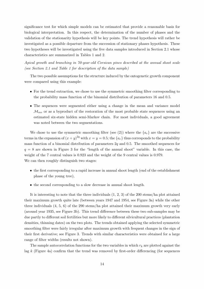
• The sequences were segmented either using a change in the mean and variance modelMmv or as a byproduct of the restoration of the most probable state sequences using anestimated six-state hidden semi-Markov chain. For most individuals, a good agreementwas noted between the two segmentations.

We chose to use the symmetric smoothing filter (see (2)) where the {ar} are the successiveterms in the expansion of (x + y)2q with x = y = 0.5; the {ar} thus corresponds to the probabilitymass function of a binomial distribution of parameters 2q and 0.5. The smoothed sequences forq = 8 are shown in Figure 3 for the “length of the annual shoot” variable. In this case, theweight of the 7 central values is 0.923 and the weight of the 9 central values is 0.979.We can then roughly distinguish two stages:

• the first corresponding to a rapid increase in annual shoot length (end of the establishmentphase of the young tree),

• the second corresponding to a slow decrease in annual shoot length.

It is interesting to note that the three individuals (1, 2, 3) of the 200 stems/ha plot attainedtheir maximum growth quite late (between years 1947 and 1954, see Figure 3a) while the otherthree individuals (4, 5, 6) of the 290 stems/ha plot attained their maximum growth very early(around year 1935, see Figure 3b). This trend difference between these two sub-samples may bedue partly to different soil fertilities but more likely to different silvicultural practices (plantationdensities, thinning dates) on the two plots. The trends obtained applying the selected symmetricsmoothing filter were fairly irregular after maximum growth with frequent changes in the sign oftheir first derivative; see Figure 3. Trends with similar characteristics were obtained for a largerange of filter widths (results not shown).

The sample autocorrelation functions for the two variables in which rk are plotted against thelag k (Figure 4a) confirm that the trend was removed by first-order differencing (for sequences

14

containing a trend, the values of rk do not come down to zero except for very large lag values).The sample autocorrelation functions of the residual sequences obtained with two different filters(first-order differencing in Figure 4a, and unweighted moving average with a half-width q = 2 -see equation (3) - in Figure 4b) are close to the autocorrelation functions induced by a white noisesequence; see Section 2.2. The roughly random local fluctuations result mainly from changingclimatic conditions over the years.

The sample cross-correlation function computed from the bivariate differenced sequences ischaracterized by a single significant correlation coefficient at lag 0 with value 0.2 (the othercorrelation coefficients for both positive and negative lags are not significantly different from 0).This illustrates the fact that the two observed variables correspond to two different biologicalphenomena.

For each individual, we applied multiple change-point detection methods both to the bivariatesequence (annual shoot length and number of branches per tier) and to the univariate sequencecorresponding solely to the annual shoot lengths. For most individuals, the segmentations wereidentical or very similar (for number of segments in the neighborhood of the optimal number ofsegments). There were some exceptions where the number of branches induced a distortion inthe segmentation. Hence, we chose to show mainly the results of multiple change-point detectionmethods applied to univariate sequences (Figures 5, 6 and 7) and simply illustrated application tobivariate sequences on the individual which showed changes of higher magnitude for the numberof branches (median diameter individual 5, 290 stems/ha plot); see Figure 8. In this case, thesecond change point is mainly explained by the number of branches (this change point is shiftedfrom three years compared to the segmentation of the univariate sequence), while the first andthird change points are mainly explained by the annual shoot length. For this individual, themBIC favors the four-segment model both in the univariate case (posterior probability of 0.73,see Table 4) and the bivariate case (posterior probability of 0.61).

We chose for each sequence the number of segments that achieves the best compromise withthe segmentation computed on the basis of the estimated six-state hidden semi-Markov chain (seebelow). Hence, the selected change-point models do not systematically correspond to the bestchange-point models according to the mBIC (Zhang and Siegmund, 2007) but rather to possiblechange-point models. For the median diameter individual 2 of the 200 stems/ha plot, we selectedthe five-segment model (with posterior probability P (M5,mv|xτ−10

) = 0.12) while the mBIC fa-vored the six-segment model (with P (M6,mv|xτ−10

) = 0.77), and for the large diameter individ-ual 4 of the 290 stems/ha plot, we selected the five-segment model (with P (M5,mv|xτ−10

) = 0.21)while the mBIC favored the four-segment model (with P (M4,mv|xτ−10

) = 0.72). For the fourother individuals, the selected change-point model corresponds to the best model according tothe mBIC; see the posterior probabilities of the selected change-point models in Tables 3 and 4.We also applied the penalized likelihood criterion proposed by Lebarbier (2005) whose penaltyterm depends on unknown constants that were calibrated by simulation. We obtained the samebest change-point models as with the mBIC except for the small diameter individual 3 of the200 stems/ha plot where Lebarbier’s criterion favored the five-segment model instead of thesix-segment model favored by the mBIC (but P (M5,mv|xτ−10

) = 0.33 on the basis of the mBIC;

15

see Table 3).A “left-right” six-state hidden semi-Markov chain composed of five successive transient states

followed by a final absorbing state was estimated on the basis of the six bivariate sequencescorresponding to the six individuals. The iterative estimation algorithm was initialized with a“left-right” model such that πj > 0 for each state j, pij = 0 for j ≤ i and pij > 0 for j > i foreach transient state i, pii = 1 and pij = 0 for j �= i for the final absorbing state. Convergenceof the iterative estimation procedure (expectation-maximization (EM) algorithm) required 16iterations. States 0 and 1 are the only possible initial states (with π0 = 0.83 and π1 = 0.17) ofthe estimated hidden semi-Markov chain. The estimated transition probability matrix is

P =

0 0.52 0.48 0 0 00 0 1 0 0 00 0 0 1 0 00 0 0 0 1 00 0 0 0 0 10 0 0 0 0 1

.

This transition probability matrix is almost degenerated, the transition probability p02 = 0.48corresponding to the three individuals of the 290 stems/ha plot for which there is no interme-diate phase between the first phase immediately after germination (state 0) and the maximumgrowth phase (state 2). A “left-right” hidden semi-Markov chain is said to be degenerated iffor each transient state i, pii+1 = 1 and pij = 0 for j �= i + 1 (and for the final absorbing statepii = 1, and pij = 0 for j �= i). It should be noted that the succession of segments is determin-istic for both a degenerated “left-right” hidden semi-Markov chain and a multiple change-pointmodel. This almost deterministic succession of states supports the assumption of a successionof growth phases. An occupancy distribution representing the length of the phase in numberof years is attached to each nonabsorbing state and two observation distributions, representing,respectively, the length of the annual shoot and the number of branches per tier within the phaseare attached to each state. The state occupancy distributions and the observation distributionsfor the two observed variables are parametric discrete distributions chosen among binomial,Poisson and negative binomial distributions with an additional shift parameter d (with d ≥ 1for the state occupancy distributions); see the Appendix. The most probable state sequencewas computed for each observed sequence using the so-called Viterbi algorithm (Guédon, 2003).The restored state sequence can be viewed as the optimal segmentation of the correspondingobserved sequence into sub-sequences with each sub-sequence corresponding to a given state.

The state frequencies extracted from the restored state sequences (i.e. the cumulated lengthof the segments for a given state) are (f0, f1, f2, f3, f4, f5) = (21, 29, 140, 87, 71, 58). Hence, onlythe occupancy distributions for the five transient states were poorly estimated which is not toodramatic since each state is well differentiated from its immediately preceding and followingstates on the basis of the observation distributions mainly for the “length of the annual shoot”variable; compare the absolute mean difference |mj+1 −mj| between consecutive states withthe standard deviations σj and σj+1 for the two observed variables in Table 5. With its almost

16

deterministic succession of states, the estimated six-state hidden semi-Markov chain is fairlyreliable even if it was estimated on the basis of only six sequences. One should keep in mindthat the objective here is not to fit adequately the data but rather to segment the observedsequences using the estimated model.

With model Mmv, the ontogenetic growth component is modeled as a piecewise constantfunction. We chose to compute for each observed sequence, a piecewise constant function onthe basis of the most probable state sequence computed using the estimated six-state hiddensemi-Markov chain (the constants are the empirical means estimated for each segment); seeFigures 5 and 6. Whatever be the segmentation method used (multiple change-point modelMmv or restoration of the most probable state sequences using the estimated six-state hiddensemi-Markov chain), change points of high magnitude were detected after maximum growth(i.e. when growth decreases); see Figures 5a,b and 6b. Change points of high magnitude werealso detected before maximum growth. The sample autocorrelation function computed fromthe residual sequences, obtained by subtracting from each original sequence the step functiondeduced from the estimated Mmv model (Lavielle, 1998), showed that the residual sequenceswere stationary and close to white noise sequences (results not shown). The change pointscorresponding to the decrease in the shoot length of highest magnitude are not synchronized(1985 → 1986 for individuals 2 and 3 but 1975 → 1976 for individual 6) and cannot be explainedby an unusual climatic year; see Figures 5, 6 and 7. Furthermore, it should be noted that the1985 → 1986 change point for individual 3 corresponds to a decrease in length of high magnitudespread over two years (1984→ 1986) (Figure 5b) and the 1985→ 1986 change point for individual2 corresponds to a decrease in length of roughly the same magnitude but spread over three years(1983 → 1986) (Figure 5a).

Apical growth and branching in young Corsican pines described at the annual shoot scale (seeSection 2.1 and Table 1 for description of the data sample)

To investigate further the succession of stationary phases assumption for the ontogeneticgrowth component, we chose to estimate a single statistical model on the basis of the four sub-samples of young Corsican pine (from 6 to 23 year old). In this way, different climatic yearsare mixed for a given ontogenetic stage. It should be noted that these four sub-samples onlycorrespond to growth increase. A “left-right” three-state hidden semi-Markov chain composedof two successive transient states followed by a final absorbing state was estimated. The para-meterization of this three-state hidden semi-Markov chain is identical to that of the six-statehidden semi-Markov chain estimated on the basis of the 70-year-old Corsican pines (two para-metric observation distributions representing, respectively, the length of the annual shoot andthe number of branches per tier within the phase are attached to each state). The iterativeestimation algorithm was initialized with a “left-right” model such that πj > 0 for each statej, pij = 0 for j ≤ i and pij > 0 for j > i for each transient state i, pii = 1 and pij = 0 forj �= i for the final absorbing state. Convergence of the iterative estimation algorithm required17 iterations. The fact that state 0 is the only possible initial state (π0 = 1) and that state 1cannot be skipped (i.e. p02 = 0) is the result of the iterative estimation procedure; see Figure

17

9. The observation distributions for the two variables are ordered in the same way, but theobservation distributions for the “length of the annual shoot” variable are more separated (lessoverlapping between observation distributions corresponding to two successive states) than theobservation distributions for the “number of branches” variable; compare the mean differencemj+1 − mj between consecutive states with the standard deviations σj and σj+1 for the twoobserved variables in Table 6.

Contrarily to multiple change-point models, there is no model selection method with a firmmathematical basis for the selection of the number of states of a non-ergodic hidden Markovianmodel. In practice, “left-right” hidden semi-Markov chains were estimated for successive numberof states and two main criteria were combined for the practical selection of the number of states:

• A non-adequate fit of an empirical marginal distribution for a given variable by the cor-responding mixture of observation distributions is generally an indicator of underparame-terization of the model.

• The fact that some states can be skipped with a high probability is an indicator of over-parameterization of the model in our application context where a deterministic successionof states supports the assumption of a succession of growth phases.

The fit of the empirical marginal distribution for the “length of the annual shoot” variableby the mixture of observation distributions is shown in Figure 10, the weight associated with anobservation distribution being the weight of the corresponding state. Each observation distrib-ution corresponds to a well-identified mode of the mixture. Hence, the three states correspondclearly to different ranges of values for the “length of the annual shoot” variable. The estimationof a mixture of distributions (McLachlan and Peel, 2000) directly from the marginal distributionfor the “length of the annual shoot” variable confirms the three component structure whateverbe the model selection criterion (AIC, BIC) used to determine the number of components of themixture. This can be viewed as a practical way of assessing the choice of the number of statesof the model. The existence of under-represented and over-represented ranges of values is not inaccordance with an underlying monotone trend (since the samples of sequences only correspondto the successive stages from germination to maximum growth stage).

The alternative assumption can be further investigated by exploring the properties of thesub-sequences extracted for the three phases. The restored state sequences (most probable statesequences computed by the Viterbi algorithm) can be used to segment the observed sequencesinto sub-sequences with each sub-sequence corresponding to a given state. Since the first yearswere not systematically observable, the time spent in state 0 may be left-censored; see thenumber of non-measured years in the data presentation for state 0 (this cannot be taken intoaccount in a non-ergodic model such as a “left-right” model). The time spent in state 1 is right-censored in 16 sequences (out of 104) while the time spent in absorbing state 2 is systematicallyright-censored. This is a direct consequence of the fact that the last year of measurement doesnot systematically coincide with a phase change. A one-way analysis of variance shows that theempirical observation distributions extracted from the restored state sequences for state 1 are

18

not significantly different for the four sub-samples. This analysis cannot be transposed to states0 and 2 since state 0 is affected by left censoring and state 2 is affected by right censoring indifferent ways depending on the sub-sample.

The pointwise average lengths of the annual shoots were computed from each sample of sub-sequences corresponding to each phase; in this way, the index parameter could be interpretedas an “ontogenetic” year. Sub-sequences extracted for state 0 were aligned on the last yearsince this state is affected by left censoring while sub-sequences extracted for states 1 and2 were aligned on the first year. We checked that the phases were sufficiently asynchronousbetween trees by extracting the first year in each phase; see Figure 11b. Hence, the calendaryears are reasonably randomized for a given ontogenetic year. Sub-sequences extracted forstates 0 and 1 do not exhibit residual trends within the phase while sub-sequences extractedfor state 2 exhibit a slowly increasing residual trend; see the pointwise means computed fromthe different samples of sub-sequences extracted for each state in Figure 11a. This is confirmedby the sample autocorrelation functions computed for the entire sequences (Figure 12a) and forthe three samples of sub-sequences corresponding to each phase (Figure 12b,c,d). It should berecalled that if sequences contain a trend, then the autocorrelation coefficients will not comedown to zero except for large lag values. This is because an observation on one side of the overallmean tends to be followed by observations on the same side of the mean because of the trend.One of the major difficulties when analyzing this type of data is that the fluctuations of climaticorigin within a phase may be of the same order of magnitude as the transitions between phases.This point can be illustrated by the annual shoot length inter-annual differences computedby first-order differencing where within-phase differences are distinguished from between-phasedifferences (Figure 13) (within-phase mean: 2.4, between-phase mean: 15.4).

Apical growth and branching in Scots pines described at the annual shoot scale (see Section 2.1and Table 1 for description of the data sample)

Applying the same approach already described for young Corsican pines, we estimated asingle statistical model on the basis of the six sub-samples of Scots pines (from 3 to 70 year old).Different climatic years are thus mixed for a given ontogenetic stage. The point of interest in thisexample is the fact that the two sub-samples of oldest trees cover growth decrease. A “left-right”five-state hidden semi-Markov chain composed of four successive transient states followed by afinal absorbing state was estimated. The iterative estimation algorithm was initialized with a“left-right” model such that πj > 0 for each state j, pij = 0 for j ≤ i and pij > 0 for j > i foreach transient state i, pii = 1 and pij = 0 for j �= i for the final absorbing state. Convergenceof the iterative estimation algorithm required 44 iterations. In the estimated model, states 0and 1 are the only possible initial states (with π0 = 0.7 and π1 = 0.3). Restoration of themost probable state sequences shows that sequences starting in state 1 belong mainly to thetwo sub-samples of oldest trees whereas the very first annual shoots corresponding to the firstphase were not observable. The fact that states cannot be skipped (i.e. for each transient statei, pii+1 = 1 and pij = 0 for j �= i + 1) is the result of the iterative estimation procedure. Eachobservation distribution for the “length of the annual shoot variable” is well separated from

19

the observation distributions corresponding to the immediately preceding and following states(since the only possible transitions are from a given state to the immediately following state), thelargest overlapping concerning the state 2 observation distribution (corresponding to maximumgrowth) with state 1 and state 3 observation distributions; compare the absolute mean difference|mj+1 −mj | between consecutive states with the standard deviations σj and σj+1 for the twoobserved variables in Table 7. It should be noted that the maximum number of branches (state1) was reached before the maximum length of the annual shoot (state 2); see Table 7.

The pointwise average lengths of the annual shoots were computed from each sample of sub-sequences extracted for each phase. We checked that the phases were sufficiently asynchronousbetween trees by extracting the first year in each phase (result not shown). Hence, the calendaryears are reasonably randomized for a given ontogenetic year. Sub-sequences extracted for states0 and 1 exhibit increasing residual trends on both sides of the transition from state 0 to state 1(which corresponds to the change of highest magnitude for the annual shoot length); see Figure14. Sub-sequences extracted for state 2 exhibit a slowly increasing then decreasing residual trendwhile sub-sequences extracted for states 3 and 4 do not exhibit residual trends within the phase.

Apical growth in sessile oaks described at the annual shoot scale (see Section 2.1 and Table 2 fordescription of the data sample)

In a first step of analysis, a two-state hidden semi-Markov chain composed of a transient statefollowed by a final absorbing state was estimated on the basis of the two sub-samples of sessileoaks (a parametric observation distribution representing the length of the annual shoot, and anonparametric observation distribution representing the number of growth units, are attachedto each state). Applying the approach already described for young Corsican pines, two samplesof sub-sequences were extracted on the basis of the restored state sequences, each correspondingto a given phase. The pointwise average lengths of the annual shoots and the pointwise averagenumbers of growth units were computed from each sample of sub-sequences corresponding to eachphase. We checked that the phases were sufficiently asynchronous between trees by extractingthe first year in each phase (result not shown). Sub-sequences extracted for state 0 both forthe “length of the annual shoot” and “number of growth units” variables and for state 1 forthe “number of growth units” variable do not exhibit residual trends (Figure 15a,b) while thesub-sequences extracted for state 1 for the “length of the annual shoot” variable exhibit a slowlyincreasing trend (Figure 15a).

Since the range of values for the “length of the annual shoot” variable in state 1 is broad- annual shoot lengths from 10 cm to 140 cm - (see the support and the dispersion of state 1observation distribution in Figure 16), we attempted to identify a supplementary structure withinthe phase corresponding to state 1, the alternative assumption being that the roughly randomvariations within the phase are mainly of climatic origin. A three-state hidden semi-Markovchain composed of a transient state followed by a two-state recurrent class was thus estimated(the absorbing state of the two-state model is thus replaced by a two-state recurrent class inthis three-state model). Since the occupancy distributions of the two recurrent states were closeto geometric distributions (Figure 17), we chose to estimate a hidden hybrid model (Guédon,

20

2005) composed of a transient semi-Markovian state followed by two recurrent Markovian states(Figure 18). The log-likelihoods of the two three-state models are close while the AIC are almostidentical and the BIC favors the hybrid model; see Table 8 where the results for the two-statehidden semi-Markov chain are also given as reference. The usage of AIC and BIC is justifiedin this case since the model comparison only concerns the final recurrent class. The estimatedtransition probability matrix for the three-state hidden hybrid model is

P =

0 1 00 0.4 0.60 0.36 0.64

.

Since the transition distributions for state 1 and state 2 are close (see the second and thethird rows of the above matrix), this two-state “order 0” recurrent class can be interpreted asa single absorbing state whose attached observation distribution is a mixture of the observationdistributions estimated for the two recurrent states; see Figure 19. It should be noted that state1 corresponds to monocyclic or bicyclic medium shoots while state 2 corresponds to bicyclicor tricyclic long shoots; see the estimated observation probability matrix below (row: state;column: number of growth units)

B =

0.84 0.14 0.02 00.56 0.4 0.04 00 0.76 0.23 0.01

.

This result tends to confirm the hypothesis of roughly random variations within the secondphase of rapid growth. We also checked that the cumulated number of growth units as a functionof the number of measured years was remarkably homogeneous (result not shown) which furtherconfirms this result.Apical growth in Dicorynia guianensis described at the internode scale (see Section 2.1 and Table2 for description of the data sample)

The main axis of the selected individual had 152 internodes and its height was 5.5 m. Forthe selection of the number of segments, we computed both the mBIC (Zhang and Siegmund,2007) and the penalized likelihood criterion proposed by Lebarbier (2005) for model Mmv. ThemBIC favored the four-segment model (with posterior probability P (M4,mv|xτ−10

) = 0.47),while Lebarbier’s criterion favored the three-segment model (but P (M3,mv|xτ−10

) = 0.25 on thebasis of the mBIC). We chose to compare three models for three segments: change in the meanmodelMm, change in the mean and variance modelMmv and change in the variance modelMv.In this latter case, a model Mv was estimated on the basis of the residual sequence computed bysubtracting from the original sequence the step function deduced from the previously estimatedmodel Mm. The empirical means estimated for the three segments of the residual sequence liebetween -1 and +1. It is not recommended to apply directly the change in the variance modelMvto the original sequence since the constant mean assumption (which is far from being verified;see Figure 20) affects strongly the estimation of the within-segment variances and consequently

21

of the change points. The estimation of the within-segment means for the change in the meanmodel Mm is far more robust regarding departure from the constant variance assumption.

One should note the similarity between the three segmentations; see Figure 20. In fact, theminimum internode length was roughly constant along the axis while the maximum internodelength changed abruptly, defining the three phases. It was therefore considered relevant to studythe relationship between the mean mj and an indicator of dispersion of the internode length fora given segment. This can be investigated with the simple linear model mj = α+βσj where theintercept α can be interpreted as the minimum internode length. It should be noted that, in thiscontext, the means mj and the variances σ2j were a posteriori estimated from the segmentationwhen they were not parameters of the multiple change-point model (variances for the change inthe mean model Mm and means for the change in variance model Mv); see the estimated valuesin Table 9. Because of the Gaussian distribution assumption, a fixed proportion of the internodelengths lies in the interval [α, 2mj − α] corresponding to mj ± βσj whatever be the segment j.Whatever be the estimation context (three segments of the change in the mean and variancemodel Mmv or nine segments extracted from the three estimated models, the linear relationshipis very strong with r2 > 0.99). We obtain α ≃ 7 and β ≃ 1.47 with small fluctuations dependingon the estimation context.

The short internodes generally define limits between growth units. This type of analysisapplied to the successive lengths of growth units would therefore give the same result. It waschecked that fluctuations in the internode lengths were not of climatic origin and we suspectthat they are expressions of endogenous equilibriums; see Hallé and Martin (1968). Accordingto the field observations, the first change point corresponded approximately to the occurrenceof the first offspring shoot (height of 45 cm) while the second change point (height of 285cm) corresponded approximately to the beginning of a more intensive branching zone. Thenumber of leaflets was 3 at the base of the axis while it reached 7 at the top of the axis,this number increasing by step of 2. An interesting open question is whether this increase inthe number of leaflets is related to the change points identified on the internode length. Allthese changes (concerning internode length, number of leaflets and branching density) may beglobally interpreted as an adaptation to changing light levels induced by stratum changes ofthe individual. For this type of tropical rain forest, from 3 to 5 plant strata corresponding tocontrasting light environments are often identified (Richards, 1998; Rijkers et al., 2000).

3 DiscussionOur starting assumption was a decomposition model where observed growth is the result of twocomponents, an ontogenetic component and an environmental component (mainly of climaticorigin in our examples). Multiple change-point models and hidden semi-Markov chains wereapplied to identify successions of growth phases on different samples of tree trunks described atthe annual shoot scale (corresponding to Corsican pines, Scots pines and sessile oaks), and onthe main axis of a Dicorynia guianensis described at the internode scale. Symmetric smoothingfilters were also applied to extract trends in the 70-year-old Corsican pines. The results sup-

22

port the assumption of abrupt changes between roughly stationary phases rather than gradualchanges. It is important to note that phase identification accuracy is strongly related to phaselength and to the magnitude of the change points that delimit the phase, the ideal situationbeing a long stationary phase delimited by two change points of high magnitude. We checkedthat the change points corresponding to the decrease in shoot length of highest magnitude werenot synchronized, thus eliminating a purely climatic origin for these abrupt changes. We alsochecked that the climatic component is roughly a random stationary component using differ-ent methods in 70-year-old Corsican pines and sessile oaks. We thus suspect that these phasechanges are expressions of endogenous equilibriums.

Concerning multivariate sequences, the examples presented illustrate two situations: theobserved variables are either indicators of a single biological phenomenon (sessile oak with lengthof the annual shoot and number of growth units for the apical growth process) or are indicatorsof different but related biological phenomena (pines with length of the annual shoot for the apicalgrowth process and number of branches per tier for the branching process). These two situationsare directly expressed in the cross-correlation coefficient at lag 0 computed from the bivariatedifferenced sequences (the ontogenetic component is thus eliminated) with r0 = 0.2 for 70-year-old Corsican pines, r0 = 0.38 for young Corsican pines, r0 = 0.14 for Scots pines and r0 = 0.59for sessile oaks. The intermediate value for young Corsican pines raises further questions but, atfirst sight, the pine case and the sessile oak case are clearly differentiated. In the case illustratedby the pine examples, there is clearly a hierarchy within the variables since the structuring insuccessive phases is mainly explained by the length of the successive annual shoots along thetrunk. An open question concerns a possible structuring in phases relying on different variablescorresponding to different biological phenomena. In maritime pine (Pinus pinaster), it has beenshown that the occurrence of axillary female cones on the trunk can be related to a decreasein trunk annual shoot length (Heuret et al., 2006) on the basis of pointwise means computedfor these two observed variables. This type of data (which includes supplementary variablessuch as the number of growth units) could be re-analyzed using the methods illustrated in thispaper in order to better characterize the successive phases. It should be noted that both hiddensemi-Markov chains and multiple change-point models with appropriate parameterizations canbe applied to multivariate sequences build from variables of heterogeneous types.

It would be interesting to consider models intermediate between our two rather extremehypotheses (trend versus succession of stationary phases). This is in theory possible but inpractice, the rather short length of some phases would render quite unreliable the estimationof a piecewise linear function by a multiple change-point detection method. Since hidden semi-Markov chains are estimated on the basis of a sample of sequences, it is more realistic to estimatein this case a linear model for each state (instead of a simple observation distribution). Theresulting model would be a semi-Markov switching linear model.

Relations with botanical notions of “phase change” and “morphogenetic gradient”The repetition of elementary botanical entities always induces changes in their morphological

characteristics. Changes are commonly recognized as gradual or abrupt and are referred to as

23

“allomorphosis” and “metamorphosis”, respectively; see Ray (1990) and Day et al. (1997). Thegradual or abrupt character of change was often a priori defined in relation to the type ofcharacteristic selected and the level of description. For instance, if the non-flowering/floweringcharacter of the entity was of interest, the first occurrence of flowers was often interpretedas an abrupt change (Doorenbos, 1954; Wareing, 1959, 1961; Zimmerman, 1972; Borchert,1976; Greenwood, 1995) defining the limit between the juvenile phase and the adult phase. Inbotany, the term “phase change” refers to the change from non-reproductive to reproductivestatus (Jones, 1999). When quantitative variables such as the length of the annual shoot wereconsidered instead of binary variables, the changes were often implicitly considered as gradual(or uninterrupted for Gatsuk et al., 1980). This in particular was the case when studyingcommon morphogenetic gradients (Barthélémy and Caraglio, 2007) such as the “base effect”,which corresponds to the first stages in the ontogeny, and the drift, which corresponds to theageing of an axis, or the more general notion of “loss of vigor” (Menzies et al., 2000); see alsoMencuccini et al. (2005) and Steele et al. (1989).

The definition of phases as a consequence of gradual or abrupt changes may be stronglyinfluenced by the nature of the underlying variable (either discrete qualitative with a smallnumber or possible values or quantitative - either count or continuous - variable). For instance,the base effect is often described as a rapid increase for different quantitative variables (lengthof the internode, length of the annual shoot, number of growth units in the case of polycyclicspecies) and the end of this phase is rather described as a stabilization (hence, corresponding tothe location of the maximum curvature in the plot (t, xt) where xt is the quantitative variableof interest). In the case of quantitative variables, the transition between phases may correspondto an abrupt change (in values) but also to a change in slope or to a maximum curvature.Generally, phase changes are explicitly defined while phases themselves are often implicitlydefined (Poethig, 1990; Jones, 1999). When explicitly defined, phases may be stationary, butmay also take the form of a slope (Souza et al., 2000; Sylvester et al., 2001). One further sourceof confusion is the fact that botanical phases may be either defined on the basis of individualsequences or on the basis of pointwise means computed from a set of sequences, assuming thatthe individual sequences are synchronous (this approach is referred to as a cross-sectional studyin statistics, the alternative approach where the individual sequences are directly consideredbeing referred to as a longitudinal study). For instance, if pointwise means are computed fromsequences characterized by asynchronous abrupt changes, these pointwise means take the formof a trend were the occurrence of abrupt changes is totally masked. In the case of a discretevariable defined on a small set of values (whatever be its nature, nominal, ordinal or count),the phase changes often correspond to changes in the distribution of the variable of interest (forinstance, some events become abruptly far less or more probable).

There are contrasting points of views for investigating, on the one hand, the first stage ofgrowth increase (from germination to maximum growth) and the second stage of growth decrease(from maximum growth to senescence). While it is often admitted that root installation (Guérardet al., 2001; Collet and Frochot, 1996) or stratum change (see the Dicorynia guianensis exampleand Sterck and Bongers, 2001) can induce an abrupt increase in the length of the entities,

24

the ageing process is often viewed as a gradual decrease (called “drift”) in the length of theentities. Hence, identifying phase changes of high magnitude when growth globally decreasesis an unexpected result. The roughly stationary character of some “long” phases (more than20 years), including the phase of maximum growth, in 70-year-old Corsican pines (Figures 5, 6and 8) raises also further questions regarding functioning hypotheses. It would be interestingto study in future works variables such as total leaf area, the number of active shoot apices orthe number of sexual organs that could explain these abrupt changes; see Section 4 for furtherdiscussion concerning the analysis of the whole plant development. One major difficulty lies inthe fact that these variables can only be estimated over short periods corresponding to the lastfew years on the basis of retrospective measurements.

Observation protocolsTwo contexts should be distinguished (see the discussion about replications for studying

stochastic processes in Lindsey, 2004, chapter 1):

• A single or a few mature trees are measured. The data thus provide an overall pictureof tree life but sufficient information is only available in the case of long and well-definedstationary phases (delimited by two change points of high magnitude); see the precedingitem in the Discussion.

• Only the most recent entities are measured in a sample of tree trunks. Sufficient informa-tion is available whatever be the length of the phases but only a few (possibly censored)phases can be studied in this way.

In our context, data were collected retrospectively, i.e. plant development was reconstitutedat a given observation date from morphological markers corresponding to past events; see Heuretet al., (2000) and Nicolini et al. (2001) for the use of pith markers. This ability to observeretrospectively topological information is a key property for plant structure analysis (planttopology is more conserved over time than plant geometry or plant biomechanical properties,for instance). Nevertheless, plant topology is affected by self-pruning and, cambial growth andbark changes obliterate morphological markers and restrict direct observation to the most recententities. In order to extract the ontogenetic growth component on the basis of a sample of shortsequences corresponding to the most recent entities, it is thus necessary to mix climatic yearswithin a given ontogenetic phase. Hence, sub-samples of trees corresponding to different ageclasses and growing under similar conditions should be observed with a specific care concerningthe overlapping of the ontogenetic phases between the different sub-samples (which both dependson the length of the sequences and the length of the ontogenetic phases, this latter informationbeing hidden). This type of observation protocol becomes rapidly quite laborious with a largenumber of measured trees.

With multiple change-point detection methods, relevant information can be extracted onthe basis of a single or a few individuals on condition that sufficiently long sequences can beobserved. This opens up new perspectives for plant architecture study where time-consuming

25

measurements and/or sophisticated technologies could be used. Examples of new variables ofinterest are:

• the diameter and insertion angle of pruned branches whose proximal part is embeddedwithin the trunk (due to cambial growth) in order to analyze branching patterns on oldparts of the tree;

• pith diameter whose changes can be related to meristem activity changes (Kaplan, 2001;Troll and Rauh, 1950);

• carbon isotope balance within the wood, which is an indicator of water availability (Dupoueyet al., 1993), and can be used to study the integrative role of the main axis.

Analysis of the influence of environmental factors on plant development taking inter-individualheterogeneity into account

In our examples, the climatic component was simply characterized globally but it may beinteresting to study in detail the plant’s response to changing climatic conditions. Markovswitching linear mixed models, i.e. models that combine linear mixed models (Searle et al.,1992; Verbeke and Molenberghs, 2000) in a Markovian manner, were introduced in Véra etal. (2004). These models belong to the family of hidden Markovian models (Ephraim andMerhav, 2002). The underlying Markov chain represents the succession of growth phases whilethe linear mixed models attached to each state of the Markov chain represent both the influenceof explanatory variables (mainly climatic variables which are time-varying explanatory variables)and inter-individual heterogeneity due to unobserved factors such as plant pathogen infestationwithin a given growth phase. This statistical modelling approach enables to differentiate the roleof environmental explanatory variables and inter-individual heterogeneity between the phases.One can assume that inter-individual heterogeneity is greater at the beginning of the plant lifewhile fluctuation amplitude mainly of climatic origin is roughly proportional to growth level.

With Markov switching linear mixed models, the response variable is constrained to beapproximately normally distributed (e.g. the annual shoot length). It would be very useful todevelop the statistical methodology for Markov switching generalized linear mixed models totake into account non-normally distributed response variables (e.g. number of growth units,number of branches, apex death/life, non-flowering/flowering character); see McCulloch andSearle (2001) and Molenberghs and Verbeke (2005) for an introduction to generalized linearmixed models.

4 Concluding remarksDifferent methods have recently been proposed for analyzing tree-structured data includingcomparison methods (Ferraro and Godin, 2000) and hidden Markovian models (Durand et al.,2005). In particular, hidden Markov tree models can be applied to identify homogeneous zones

26

within a whole plant in the same way that hidden semi-Markov chains have been applied toidentify homogeneous zones along tree trunks. The results presented in this paper and those ofthe analysis of whole plant structures presented in Durand et al. (2005) favor the hypothesis ofa small set of well-separated categories of botanical entities at the growth unit or annual shootscale. These results were obtained in contrasted species (pines, sessile oak, apple tree, etc.) withdiverse characteristics attached to the elementary botanical entities (length, number of nodes,number of growth units, number of branches, non-flowering/flowering character), these botanicalentities being either built by the same meristem or derived from one another by branching. Theseresults can be related to the notion of “physiological age of a meristem”. The physiological ageof a meristem may be defined by a particular combination of morphological, anatomical andfunctional characteristics of a given botanical entity produced by this meristem (Barthélémy etal., 1997; Barthélémy and Caraglio, 2007). For identifying the physiological age of plant entities,it seems at first sight most relevant to analyze directly the whole plant structure described ata given scale using appropriate analysis methods. The drawback with this approach is that thepanoply of analysis methods is far less developed for tree-structured data than for sequences.Hence, it is still relevant to analyze sequences extracted from plant structure, especially whenplant structure is strongly organized around a “main axis”. This is the case for all the examplespresented in this paper including the 70-year-old Corsican pines. In sequence descriptions, thevariables qualify either parent entities belonging to the sequence (length or number of internodesfor growth units for example) or offspring entities (number of branches for example). This lattercase can be further extended by qualifying not only the first-order borne entities but moregenerally the entire borne branching systems (possible variables may be maximum branchingorder, presence/absence of a reiterated branching system, a qualification of the sexual statusof the borne branching system, etc.). When analyzing a whole plant structure, it is often veryuseful to apply sequence analysis methods on paths extracted from the plant structure identifiedby tree-structured data analysis methods.

Another avenue for future works would be to investigate the relationship between primarygrowth of the trunk, as given by the length of its successive annual shoots, and secondary orcambial growth, as given by the successive annual ring areas. While cambial growth of the trunkintegrates the whole tree development, primary growth of the trunk is simply assumed to reflectwhole tree development in the case of a “young” tree with a strong hierarchical organization.

All the data samples presented in this paper were analyzed with the V-Plants software whichis freely available at http://www-sop.inria.fr/virtualplants.

AcknowledgmentsThe authors thank Evelyne Costes and a rewiever for their helpful comments that led to an

improvement in the presentation of this paper.

ReferencesAuger, I. E., Lawrence, C. E., 1989. Algorithms for the optimal identification of segment neigh-borhoods. Bull. Math. Biol. 51, 39-54.

27

Barthélémy D., 1991. Levels of organization and repetition phenomena in seeds plants. ActaBiotheoretica 39, 309-323.Barthélémy, D., Caraglio, Y., Costes, C., 1997. Architecture, gradients morphogénétiques etâge physiologique chez les végétaux. In: Bouchon, J., de Reffye, P., Barthélémy, D. (Eds.),Modélisation et Simulation de l’Architecture des Végétaux, Science Update, INRA éditions,Paris, pp. 89-136.Barthélémy, D., Caraglio, Y., 2007. Plant morphology and architecture: A dynamic, multi-level and comprehensive approach of plant form and ontogeny. Ann. Bot. 99(3), 375-407.doi:10.1093/aob/mcl260.Borchert, R., 1976. The concept of juvenility in woody plants. Acta Horticulturae 56, 21-33.Box, G. E. P., Jenkins, G. M., Reinsel, G. C., 1994. Time Series Analysis, Forecasting andControl, 3rd edn. Prentice-Hall, Englewood Cliffs.Braun, J. V., Müller, H.-G., 1998. Statistical methods for DNA sequence segmentation. Statist.Sci. 13(2), 142-162.Brockwell, P. J., Davis, R. A., 2002. Introduction to Time Series and Forecasting, 2nd edn.Springer, New York.Burge, C., Karlin, S., 1997. Prediction of complete gene structures in human genomic DNA. J.Mol. Biol. 268, 78-94.Caraglio, Y., Barthélémy, D., 1997. Revue critique des termes relatifs à la croissance et à laramification des tiges des végétaux vasculaires. In: Bouchon, J., de Reffye, P., Barthélémy,D., (Eds.), Modélisation et Simulation de l’Architecture des Végétaux, Science Update, INRAéditions, Paris, pp. 11-87.Chatfield, C., 2003. The Analysis of Time Series: An Introduction, 6th edn. Chapman &Hall/CRC Press, Boca Raton.Collet, C., Frochot, H., 1996. Effects of interspecific competition on periodic shoot elongationin oak seedlings. Can. J. Forest Res. 26(11), 1934-1942.Day, J. S., Gould, K. S., Jameson, P. E., 1997. Vegetative architecture of Elaeocarpushookeri-anus: transition from juvenile to adult. Ann. Bot. 79, 617—624.Diggle, P. J., 1990. Time Series: A Biostatistical Introduction. Oxford University Press, Oxford.Diggle, P. J., Heagerty, P., Liang, K.-Y., Zeger, S. L., 2002. Analysis of Longitudinal Data, 2ndedn. Oxford University Press, Oxford.Drénou, C., 1994. Approche architectural de la scenesence des arbres: Le cas de quelquesangiospermes temperées et tropicales. PhD thesis, Université Montpellier II.Doorenbos, J., 1954. Rejuvenation of Hedera helix in grafts combinations. In: ProceedingsKoninklijke Nederlandse Akademie van Wetenschappen Ser. C 57, pp. 99-102.Dupouey, J. L., Leavitt, S., Choisnel, E., Jourdain, S., 1993. Modelling carbon isotope frac-tionation in tree rings based on effective evapotranspiration and soil water status. Plant CellEnviron. 16, 939—947.Durand, J.-B., Guédon, Y., Caraglio, Y., Costes, E., 2005. Analysis of the plant architecture viatree-structured statistical models: The hidden Markov tree models. New Phytol. 166, 813-825.

28

Ephraim, Y., Merhav, N., 2002. Hidden Markov processes. IEEE Trans. Inform. Theory 48(6),1518-1569.Ferraro, P., Godin, C., 2000. A distance measure between plant architectures. Ann. Forest Sci.57, 445-461.Fritts, H. C., 1976. Tree Rings and Climate. Academic Press, London.Gatsuk L. E., Smirnova O. V., Vorontzova L. I., Zaugolnova L. B., Zhukova L. A., 1980. Agestates of plants of various growth forms: a review. J. Ecol. 68, 675-696.Greenwood, M. S., 1995. Juvenility and maturation in conifers: current concepts. Tree Physiol.15, 433-438.Guédon, Y., 2003. Estimating hidden semi-Markov chains from discrete sequences. J. Comput.Graphical Statist. 12(3), 604-639. doi: 10.1198/1061860032030.Guédon, Y., 2005. Hidden hybrid Markov/semi-Markov chains. Comput. Statist. Data Anal.49(3), 663-688. doi:10.1016/j.csda.2004.05.033.Guédon, Y., Barthélémy, D., Caraglio, Y., Costes, E., 2001. Pattern analysis in branching andaxillary flowering sequences. J. Theor. Biol. 212, 481-520. doi:10.1006/jtbi.2001.2392.Guérard, N., Barthélémy, D., Cabanettes, A., Courdier, F., Trichet, P., Willm, J., 2001. Influ-ence de la compétition herbacée sur la croissance et le développement de jeunes Chênes rougesd’Amérique (Quercus rubra L., Fagaceae) en plantation. Ann. Forest Sci. 58, 395-410.Hallé, F., Martin, R., 1968. Etude de la croissance rythmique chez l’hévéa Hevea brasiliensisMull.-Arg. Euphorbiacées-crotonoïdées. Adansonia 8, 475-503.Heuret, P., Barthélémy, D., Nicolini, E., Atger, C., 2000. Analyse des composantes de la crois-sance en hauteur et de la formation du tronc chez le chêne sessile (Quercus petraea (Matt.)Liebl., Fagaceae) en sylviculture dynamique. Can. J. Bot. 78, 361-373.Heuret, P., Meredieu, C., Coudurier, T., Courdier, F., Barthélémy, D., 2006. Ontogenetic trendsin the morphological features of main stem annual shoots of Pinus pinaster (Pinaceae). Am. J.Bot. 93, 1577-1587.Jones, C. S., 1999. An essay on juvenility, phase change and heteroblasty in seed plants. Int. J.Plant Sci. 160(6 Suppl.), S105-S111.Kaplan, D. R., 2001. The science of plant morphology: definition, history and role in modernbiology. Am. J. Bot. 88(10), 1711-1741.Kendall, M. G., Stuart, A., Ord, J. K., 1983. The Advanced Theory of Statistics, Vol. III. Designand Analysis, and Time-Series, 4th edn. Charles Griffin, London.Kulkarni, V. G., 1995. Modeling and Analysis of Stochastic Systems. Chapman & Hall, London.Lavielle, M., 1998. Optimal segmentation of random processes. IEEE Trans. Signal Process.46(5), 1365-1373.Lavielle, M., 2005. Using penalized contrasts for the change-point problem. Signal Process.85(8), 1501-1510. doi:10.1016/j.sigpro.2005.01.012.Lebarbier, E., 2005. Detecting multiple change-points in the mean of Gaussian process by modelselection. Signal Process. 85(4), 717-736. doi:10.1016/j.sigpro.2004.11.012.Lindsey, J. K., 2004. Statistical Analysis of Stochastic Processes in Time. Cambridge UniversityPress, Cambridge.

29

Lukashin, A. V., Borodovsky, M., 1998. GeneMark.hmm: new solutions for gene finding. NucleicAcids Res. 26(4), 1107-1115.McCulloch, C. E., Searle, S. R., 2001. Generalized, Linear and Mixed Models. Wiley, New York.McLachlan, G. J., Peel, D., 2000. Finite Mixture Models. Wiley, New York.Mencuccini, M., Martinez-Vilalta, J., Vanderklein, D., Hamid, H. A., Korakaki, E., Lee, S.,Michiels, B., 2005. Size-mediated ageing reduces vigour in trees. Ecol. Lett. 8, 1183-1190.Menzies, M. I., Dibley, M. J., Faulds, T., Aimers-Hallyday, J., Holden, D. G., 2000. Mor-phological markers of physiological age for Pinus radiata. New Zeal. J. Forest. Sci. 30(3),359-364.Meredieu, C., Colin, F., Hervé, J. C., 1998. Modelling branchiness of Corsican Pine with mixed-effects models (Pinus nigra ssp. laricio). Annales des Sciences Forestières 55, 359-374.Molenberghs, G., Verbeke, G., 2005. Models for Discrete Longitudinal Data. Springer, NewYork.Monserud, R. A., 1986. Time-series analyses of tree-ring chronologies. Forest Sci. 32(2), 349-372.Nicolini, E., Caraglio, Y., Pélissier, R., Leroy, C., Roggy, J. C., 2003. Epicormic branches: agrowth indicator for the tropical forest tree, Dicorynia guianensis Amshoff (Caesalpiniaceae).Ann. Bot. 92, 97-105.Nicolini, E., Chanson, B., Bonne, F., 2001. Stem growth and epicormic branch formation inunderstorey Beech trees (Fagus sylvatica L.). Ann. Bot. 87(6), 737-750.Picard, F., Robin, S., Lavielle, M., Vaisse, C., Daudin, J.-J., 2005. A statistical approach forarray CGH data analysis. BMC Bioinformatics 6(27).Poethig, R. S., 1990. Phase change and the regulation of shoot morphogenesis in plants. Science250, 923-930.Ray, T. S., 1990. Metamorphosis in the Araceae. Am. J. Bot. 77, 1599—1609.Richards, P. W., 1998. The Tropical Rain Forest. Cambridge University Press, Cambridge.Rijkers, T., Pons, T. L., Bongers, F., 2000. The effect of tree height and light availability onphotosynthetic leaf traits of four neotropical species differing in shade tolerance. Funct. Ecol.14 (1), 77—86.Schmidler, S. C., Liu, J. S., Brutlag, D. L., 2000. Bayesian segmentation of protein secondarystructure. J. Comput. Biol. 7(1/2), 233-248.Schweingruber, F. H., 1988. Basics and Applications of Dendrochronology. Kluwer AcademicPublishers, Dordrecht, Holland.Searle, S. R., Casella, G., McCulloch, C. E., 1992. Variance Components. Wiley, New York.Souza, A. F., Martins, F. R., Silva Matos, D. M., 2000. Detecting ontogenetic stages of thepalm Attalea humilis in fragments of the Brazilian Atlantic forest. Can. J. Bot. 78, 1227—1237.Steele, M. J., Coutts, M. P., Yeoman, M. M., 1989. Developmental changes in Sitka spruce asindices of physiological age. I. Changes in needle morphology. New Phytol. 113, 367-375.Sterck, F. J., Bongers, F., 2001. Crown development in tropical rain forest trees: Patterns withtree height and light availability. J. Ecol. 89, 1-13.Sylvester, A. W., Parker-Clark, V., Murray, G. A., 2001. Leaf shape and anatomy as indicatorsof phase change in the grasses: comparison of maize, rice, and bluegrass. Am. J. Bot. 88(12),

30

2157—2167.Troll, W., Rauh, W., 1950. Das Erstarkungswachstum krautiger Dikotylen, mit besondererBerücksichtigung der primären Verdickungsvorgänge. Sitzungsberichte der Heidelberger AkademiederWissenschaften. Mathematisch- naturwissentschaftliche Klasse. Jahrgang 1950. 1 Abhandlung.1—86.Véra, C., Guédon, Y., Lavergne, C., Caraglio, Y., 2004. Analysis of longitudinal data applied toplant architecture study In: 4th International Workshop on Functional-Structural Plant Models,Montpellier, pp. 65-69.Verbeke, G., Molenberghs, G., 2000. Linear Mixed Models for Longitudinal Data. Springer,New York.Wareing, P. F., 1959. Problems of juvenility and flowering in trees. J. Linnean Soc. London,Botany 56, 282-289.Wareing, P. F., 1961. Juvenility and induction of flowering. Recent Adv. Bot. 2: 1652-1654.Zhang, N. R., Siegmund, D. O., 2007. A modified Bayes information criterion with applica-tions to the analysis of comparative genomic hybridization data. Biometrics 63, 22-32. doi:10.1111/j.1541-0420.2006.00662.x.Zimmerman, R.H., 1972. Juvenility and Flowering in Woody Plants: a Review. Hortscience 7(5), 447-455.

31

AppendixLet {St} be a discrete-time Markovian model with finite state space {0, . . . , J − 1}; see

Kulkarni (1995) for a general reference about Markov and semi-Markov models. A J-stateMarkov chain is defined by the following parameters:

• initial probabilities πj = P (S0 = j) with ∑j πj = 1,

• transition probabilities pjk = P (St+1 = k|St = j) with ∑k pjk = 1.

One drawback with Markov chains is the inflexibility in describing the time spent in a givenstate since the implicit occupancy (or sojourn time) distribution of a nonabsorbing state j is the“1-shifted” geometric distribution with parameter 1 − pjj

dj (u) = (1 − pjj) pu−1jj , u = 1, 2, . . .

This geometric distribution assumption is rarely realistic for the modelling of the length ofhomogeneous zones. A useful generalization in this context lies in the class of semi-Markovchains, in which the process moves out of a given state according to an embedded Markovchain with self-transitions in nonabsorbing states pjj = 0 and where the time spent in a givennonabsorbing state is modeled by an explicit occupancy distribution.

In the following, we define the family of hybrid Markov/semi-Markov chains which encom-passes as particular cases Markov chains and semi-Markov chains. For a hybrid Markov/semi-Markov chain, the initial probabilities are defined as for a Markov chain (see above) and thetransition probabilities are defined as follows:

• semi-Markovian state j: for each k �= j, pjk = P (St+1 = k|St+1 �= j, St = j) with∑k �=j pjk =

1 and pjj = 0,• Markovian state j: pjk = P (St+1 = k|St = j) with ∑

k pjk = 1.It should be noted that absorbing states are Markovian by definition (a state is said to beabsorbing if after entering this state it is impossible to leave it).An explicit occupancy distribution is attached to each semi-Markovian state

dj (u) = P (St+u+1 �= j, St+u−v = j, v = 0, . . . , u− 2|St+1 = j, St �= j) , u = 1, 2, . . .

In the following, we define as possible parametric state occupancy distributions binomialdistributions, Poisson distributions and negative binomial distributions with an additional shiftparameter d (d ≥ 1) which defines the minimum sojourn time in a given state.

The binomial distribution with parameters d, n and p (q = 1 − p), B(d, n, p) where 0 ≤ p ≤ 1,is defined by

dj (u) =(n− du− d

)pu−dqn−u, u = d, d + 1, . . . , n. (6)

32

The Poisson distribution with parameters d and λ, P(d, λ), where λ is a real number (λ > 0),is defined by

dj (u) = e−λλu−d

(u− d)! , u = d, d + 1, . . . (7)The negative binomial distribution with parameters d, r and p , NB(d, r, p), where r is a real

number (r > 0) and 0 < p ≤ 1, is defined by

dj (u) =(u− d + r − 1

r − 1)prqu−d, u = d, d + 1, . . . (8)

If the process starts out at t = 0 in a given semi-Markovian state j, the following relation isverified

P (St �= j, St−v = j, v = 1, . . . , t) = dj (t)πj. (9)Relation (9) means that the process enters a “new” state at time 0.

Hybrid Markov/semi-Markov chains can be seen as a sub-class of semi-Markov chains wherethe occupancy distributions of some nonabsorbing states are constrained to be geometric distri-butions.

A hidden hybrid Markov/semi-Markov chain can be viewed as a pair of stochastic processes{St,Xt} where the “output” process {Xt} is related to the “state” process {St}, which is afinite-state hybrid Markov/semi-Markov chain, by a probabilistic function or mapping denotedby f (hence Xt = f (St)). Since the mapping f is such that f (j) = f (k) may be satisfied forsome different j, k, that is, a given output may be observed in different states, the state process{St} is not observable directly but only indirectly through the output process {Xt}. This outputprocess {Xt} is related to the hybrid Markov/semi-Markov chain {St} by the observation (oremission) probabilities

bj (y) = P (Xt = y|St = j) with ∑ybj (y) = 1.

The definition of observation probabilities expresses the assumption that the output processat time t depends only on the underlying hybrid Markov/semi-Markov chain at time t. In thecase of a small set of possible outputs, the observation probabilities are directly estimated (non-parametric modelling). In the case of a larger set of possible outputs (assumed to be generatedby an interval-scaled variable), parametric observation distributions such as (6), (7) or (8) areestimated (in this context, the binomial, the Poisson or the negative binomial distributions maybe unshifted). The extension to the multivariate case is straightforward since, in this latter case,the elementary observed variables at time t are assumed to be conditionally independent giventhe state St = st.

The maximum likelihood estimation of the parameters of a hidden hybrid Markov/semi-Markov chain requires an iterative optimization technique, which is an application of the EM

33

algorithm (Guédon 2003; 2005). Once a hidden hybrid Markov/semi-Markov chain has beenestimated, the most probable state sequence can be computed for each observed sequence usingthe so-called Viterbi algorithm (Guédon, 2005). In our application context, the most probablestate sequence can be interpreted as the optimal segmentation of the corresponding observedsequence into successive ontogenetic phases.

34

Table 1. Characteristics of the data samples

Seventy-year-oldCorsican pines Young Corsican pines Scots pines

No. of sequences 6 (66 → 68) 103 76(length range) 6 year old: 31 (6) 3 year old: 32 (3)

12 year old: 29 (9 → 11) 12 year old: 10 (7 → 10)18 year old: 30 (15 → 17) 15 year old: 10 (11 → 15)23 year old: 13 (20 → 21) 30 year old: 16 (21 → 27)

40 year old: 6 (33 → 36)70 year old: 2 (47 → 67)

First variable Annual shoot length (cm) Annual shoot length (cm) Annual shoot length (cm)range, m,σ 5 → 90, 44.09, 18.15 0 → 85, 31.82, 20.73 0 → 91, 46.63, 21.33Second variable Number of branches Number of branches Number of branchesrange, m,σ 0 → 13, 5.2, 1.91 0 → 11, 5.03, 1.89 0 → 12, 5.73, 2.03

Table 2. Characteristics of the data samplesDicorynia

Sessile oaks guianensisNo. of sequences 66 1 (152)(length range) 15 year old: 46 (10 → 15)

29 year old: 20 (15 → 24)First variable Annual shoot length (cm) Internode length (mm)range, m,σ 1 → 148, 38.04, 26.42 5 → 170, 36.18, 33.06Second variable Number of growth unitsrange, m,σ 1 → 4, 1.81, 0.67

Table 3. Seventy-year-old Corsican pines, 200 stems/ha plot: Gaussian change-point modelselection (change in the mean and variance) - PJ abbreviates P (MJ,mv|xτ−10

) -.Free 1 2 3

J param. 2 logLJ mBICJ PJ 2 logLJ mBICJ PJ 2 logLJ mBICJ PJ1 2 -555.34 -567.9 0 -594.17 -606.83 0 -571.62 -584.27 02 5 -514.46 -542.26 0 -550.51 -577.89 0 -529.18 -556.55 03 8 -482.74 -524.4 0 -518.12 -559.76 0 -490.51 -533.15 04 11 -462.11 -518.97 0.02 -470.22 -527.47 0.01 -466.94 -523.03 0.015 14 -441.79 -511.92 0.55 -449.38 -520.09 0.12 -445.05 -515.14 0.336 17 -429.66 -513.29 0.28 -431.39 -516.37 0.77 -429.42 -514.31 0.497 20 -417.05 -514.9 0.12 -422.88 -521.12 0.07 -418.11 -516.63 0.158 23 -408.27 -519.18 0.01 -410.48 -523.62 0.02 -409.09 -521.05 0.029 26 -394.58 -518.76 0.02 -398.56 -524.86 0.01 -400.41 -526.41 010 29 -386.64 -524.63 0 -389.35 -528.3 0 -391.39 -530.83 0

35

Table 4. Seventy-year-old Corsican pines, 290 stems/ha plot: Gaussian change-point modelselection (change in the mean and variance) - PJ abbreviates P (MJ,mv|xτ−10

) -.Free 4 5 6

J param. 2 logLJ mBICJ PJ 2 logLJ mBICJ PJ 2 logLJ mBICJ PJ1 2 -618.48 -631.14 0 -568.92 -581.58 0 -564.84 -577.5 02 5 -553.26 -581.41 0 -521.17 -549.13 0 -498.89 -526.82 0.193 8 -521.21 -564.31 0 -470.76 -512.68 0.01 -486.46 -528.09 0.14 11 -493.88 -550.61 0.72 -447.94 -504.81 0.73 -467.79 -524.39 0.645 14 -481.98 -553.12 0.21 -437.39 -508.09 0.14 -459.27 -529.29 0.056 17 -471.37 -555.68 0.06 -425.24 -508.59 0.11 -447.05 -531.59 0.027 20 -461.27 -559.93 0.01 -417.62 -514.18 0.01 -438.19 -536.18 08 23 -451.45 -563.26 0 -408.21 -519.34 0 -430.79 -542.1 09 26 -444.15 -569.06 0 -398.63 -522.98 0 -424.18 -548.67 010 29 -436.74 -575.1 0 -392.54 -530.44 0 -417.66 -555.97 0

Table 5. Seventy-year-old Corsican pines: mean and standard-deviation of the observationdistributions of the estimated hidden semi-Markov chain.

State 0 1 2 3 4 5Annual shoot length (mj, σj) 20.83, 7.51 39.45, 7.65 62.24, 9.49 47.11, 6.94 35.07, 9.79 17.79, 6.4Number of branches (mj, σj) 4.02, 1.15 5.13, 1.36 6.7, 1.88 5.02, 1.31 4.46, 1.5 3.23, 1.22

Table 6. Young Corsican pines: mean and standard-deviation of the observation distributionsof the estimated hidden semi-Markov chain.

State 0 1 2Annual shoot length (mj, σj) 6.79, 3.21 25.04, 9.13 53.49, 11.63Number of branches (mj, σj) 3, 1.56 5.03, 1.49 6.25, 1.64

Table 7. Scots pines: mean and standard-deviation of the observation distributions of theestimated hidden semi-Markov chain.State 0 1 2 3 4Annual shoot length (mj, σj) 7.11, 5.57 40.81, 12.15 63.29, 10.35 46.51, 8.46 23.1, 10.43Number of branches (mj, σj) 3.66, 2.15 6.97, 2.07 6.37, 1.62 5.22, 1.12 3.48, 1.91

Table 8. Sessile oaks: Comparison of hidden Markovian modelsFree param. 2 logL AIC BIC

Two-state hidden semi-Markov chain 13 -10879.5 -10905.5 -10969.9Three-state hidden semi-Markov chain 23 -10562.4 -10608.4 -10722.4Three-state hidden hybrid model 20 -10568.5 -10608.5 -10707.6

36

Table 9. Dicorynia guianensis: Change points for different models (the means mj and thevariances σ2j were a posteriori estimated from the segmentation when they were not parametersof the multiple change-point model).

m0, σ0 t1 m1, σ1 t2 m2, σ2Mean 12.5, 4.71 44 31.86, 15.95 114 71.58, 43.74Mean/variance 11.54, 3.61 39 31.07, 15.75 114 71.58, 43.74Variance 11.54, 3.61 39 32.91, 17.57 118 72.06, 45.99

37

0

10

20

30

40

50

60

70

80

90

1927 1932 1937 1942 1947 1952 1957 1962 1967 1972 1977 1982 1987 1992Year

Leng

th (cm

)

123456

Figure 1. Seventy-year-old Corsican pines: Length of the annual shoots.

38

3

4

4

4

4

53

4

Etc.

4

332

3

4

55

4

5

3

4

4

4

4

53

4

Etc.

4

332

3

4

55

4

5

3

4

4

4

4

53

4

Etc.

4

332

3

4

55

4

5

Figure 2: Measurements (length of the annual shoot and number of branches per tier) on aScots pine trunk.

39

(a) 200 stems/ha plot

0

10

20

30

40

50

60

70

80

1927 1932 1937 1942 1947 1952 1957 1962 1967 1972 1977 1982 1987 1992Year

Leng

th (cm

)

123

(b) 290 stems/ha plot

0

10

20

30

40

50

60

70

80

1927 1932 1937 1942 1947 1952 1957 1962 1967 1972 1977 1982 1987 1992Year

Leng

th (cm

)

456

(a) 200 stems/ha plot

0

10

20

30

40

50

60

70

80

1927 1932 1937 1942 1947 1952 1957 1962 1967 1972 1977 1982 1987 1992Year

Leng

th (cm

)

123

(b) 290 stems/ha plot

0

10

20

30

40

50

60

70

80

1927 1932 1937 1942 1947 1952 1957 1962 1967 1972 1977 1982 1987 1992Year

Leng

th (cm

)

456

Figure 3. Seventy-year-old Corsican pines: Smoothed length of the annual shoots.

40

(a) First-order differencing

-0.6

-0.4

-0.2

0

0.2

0.4

0.6

0.8

1

0 1 2 3 4 5 6 7 8 9 10

Lag

Auto

corre

latio

n co

effic

ient

shoot lengthnumber of brancheswhite noiserandomness 95% confidence limit

(b) Unweighted moving average (q = 2)

-0.6

-0.4

-0.2

0

0.2

0.4

0.6

0.8

1

0 1 2 3 4 5 6 7 8 9 10

Lag

Aut

ocor

relat

ion

coef

ficien

t

shoot lengthnumber of brancheswhite noiserandomness 95% confidence limit

(a) First-order differencing

-0.6

-0.4

-0.2

0

0.2

0.4

0.6

0.8

1

0 1 2 3 4 5 6 7 8 9 10

Lag

Auto

corre

latio

n co

effic

ient

shoot lengthnumber of brancheswhite noiserandomness 95% confidence limit

(b) Unweighted moving average (q = 2)

-0.6

-0.4

-0.2

0

0.2

0.4

0.6

0.8

1

0 1 2 3 4 5 6 7 8 9 10

Lag

Aut

ocor

relat

ion

coef

ficien

t

shoot lengthnumber of brancheswhite noiserandomness 95% confidence limit

Figure 4. Seventy-year-old Corsican pines: Sample autocorrelation functions computed fromresidual sequences.

41

(a) Median diameter individual 2

0

10

20

30

40

50

60

70

80

90

1927 1932 1937 1942 1947 1952 1957 1962 1967 1972 1977 1982 1987 1992Year

Leng

th (cm

) datachange pointsHSMCsmoothing

(b) Small diameter individual 3

0

10

20

30

40

50

60

70

80

1927 1932 1937 1942 1947 1952 1957 1962 1967 1972 1977 1982 1987 1992Year

Leng

th (cm

) datachange pointsHSMCsmoothing

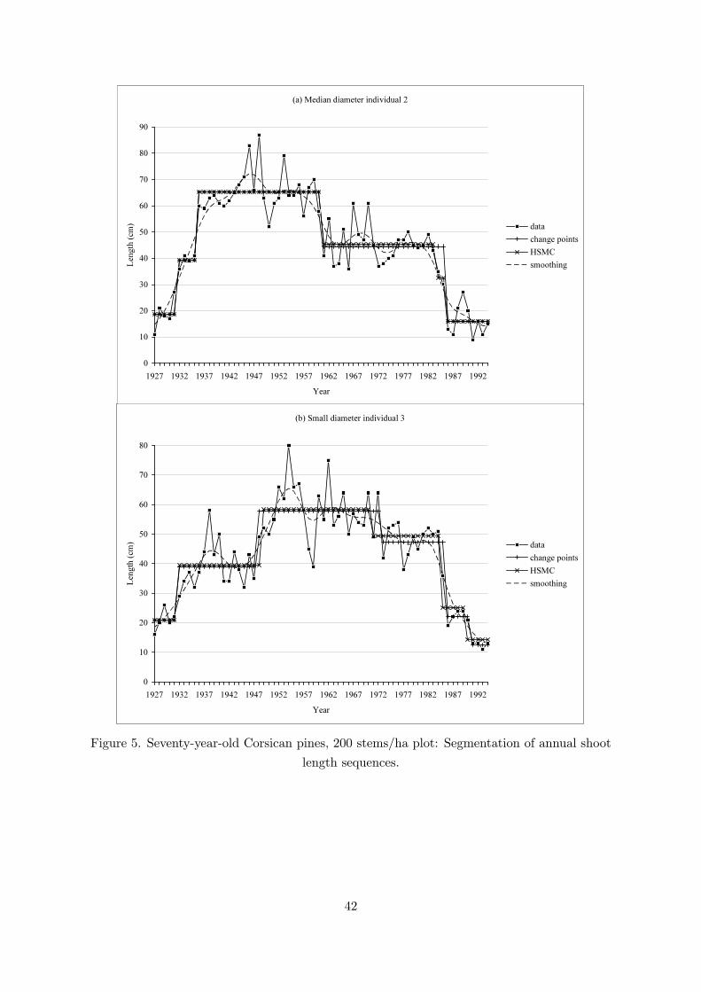
(a) Median diameter individual 2

0

10

20

30

40

50

60

70

80

90

1927 1932 1937 1942 1947 1952 1957 1962 1967 1972 1977 1982 1987 1992Year

Leng

th (cm

) datachange pointsHSMCsmoothing

(b) Small diameter individual 3

0

10

20

30

40

50

60

70

80

1927 1932 1937 1942 1947 1952 1957 1962 1967 1972 1977 1982 1987 1992Year

Leng

th (cm

) datachange pointsHSMCsmoothing

Figure 5. Seventy-year-old Corsican pines, 200 stems/ha plot: Segmentation of annual shootlength sequences.

42

(a) Large diameter individual 4

0

10

20

30

40

50

60

70

80

90

1927 1932 1937 1942 1947 1952 1957 1962 1967 1972 1977 1982 1987 1992Year

Leng

th (cm

) datachange pointsHSMCsmoothing

(b) Small diameter individual 6

0

10

20

30

40

50

60

70

80

1927 1932 1937 1942 1947 1952 1957 1962 1967 1972 1977 1982 1987 1992Year

Leng

th (cm

) datachange pointsHSMCsmoothing

(a) Large diameter individual 4

0

10

20

30

40

50

60

70

80

90

1927 1932 1937 1942 1947 1952 1957 1962 1967 1972 1977 1982 1987 1992Year

Leng

th (cm

) datachange pointsHSMCsmoothing

(b) Small diameter individual 6

0

10

20

30

40

50

60

70

80

1927 1932 1937 1942 1947 1952 1957 1962 1967 1972 1977 1982 1987 1992Year

Leng

th (cm

) datachange pointsHSMCsmoothing

Figure 6. Seventy-year-old Corsican pines, 290 stems/ha plot: Segmentation of annual shootlength sequences.

43

(a) 200 stems/ha plot

0

10

20

30

40

50

60

70

1927 1932 1937 1942 1947 1952 1957 1962 1967 1972 1977 1982 1987 1992Year

Leng

th (cm

)

1 (5)2 (5)3 (6)

(b) 290 stems/ha plot

0

10

20

30

40

50

60

70

1927 1932 1937 1942 1947 1952 1957 1962 1967 1972 1977 1982 1987 1992Year

Leng

th (cm

)

4 (5)5 (4)6 (4)

(a) 200 stems/ha plot

0

10

20

30

40

50

60

70

1927 1932 1937 1942 1947 1952 1957 1962 1967 1972 1977 1982 1987 1992Year

Leng

th (cm

)

1 (5)2 (5)3 (6)

(b) 290 stems/ha plot

0

10

20

30

40

50

60

70

1927 1932 1937 1942 1947 1952 1957 1962 1967 1972 1977 1982 1987 1992Year

Leng

th (cm

)

4 (5)5 (4)6 (4)

Figure 7. Seventy-year-old Corsican pines: Change-point model segmentations.

44

(a) Annual shoot length

0

10

20

30

40

50

60

70

80

1927 1932 1937 1942 1947 1952 1957 1962 1967 1972 1977 1982 1987 1992Year

Leng

th (cm

)

databivariate modelunivariate model

(b) Number of branches per tier

0

2

4

6

8

10

12

14

1927 1932 1937 1942 1947 1952 1957 1962 1967 1972 1977 1982 1987 1992Year

Numb

er of

branc

hes

databivariate model

(a) Annual shoot length

0

10

20

30

40

50

60

70

80

1927 1932 1937 1942 1947 1952 1957 1962 1967 1972 1977 1982 1987 1992Year

Leng

th (cm

)

databivariate modelunivariate model

(b) Number of branches per tier

0

2

4

6

8

10

12

14

1927 1932 1937 1942 1947 1952 1957 1962 1967 1972 1977 1982 1987 1992Year

Numb

er of

branc

hes

databivariate model

Figure 8. Seventy-year-old Corsican pines, median diameter individual 5, 290 stems/ha plot:Segmentation of the bivariate sequence.

45

1 20

NB(1, 3.3, 0.44)

0

0.1

0.2

0 5 10 15 20

B(1, 6, 0.36)

0

0.2

0.4

0 2 4 6

1 20 1 220

NB(1, 3.3, 0.44)

0

0.1

0.2

0 5 10 15 20

B(1, 6, 0.36)

0

0.2

0.4

0 2 4 6

Figure 9. Young Corsican pines: Estimated underlying semi-Markov chain. Each state isrepresented by a vertex which is numbered. Vertices representing transient states are edged bya single line while the vertex representing the final absorbing state is edged by a double line.The possible transitions between states are represented by arcs (the attached probabilities

which are always equal to 1 are not figured). The arc entering in state 0 indicates that it is theonly possible initial state (the attached initial probability equal to 1 is not figured). Theoccupancy distributions of the nonabsorbing states are figured above the corresponding

vertices.

46

0

0.1

0.2

0.3

0.4

0.5

0.6

0.7

0.8

0.9

1

0 5 10 15 20 25 30 35 40 45 50 55 60 65 70 75 80 85 90 95Shoot length (cm)

Cumu

lative

distr

ibutio

n fun

ction

datamixture

0

10

20

30

40

50

0 5 10 15 20 25 30 35 40 45 50 55 60 65 70 75 80 85 90 95Shoot length (cm)

Frequ

ency

datastate 0, NB(0, 12.8, 0.65)state 1, NB(0, 10.5, 0.3)state 2, NB(0, 34.4, 0.39)mixture

0

0.1

0.2

0.3

0.4

0.5

0.6

0.7

0.8

0.9

1

0 5 10 15 20 25 30 35 40 45 50 55 60 65 70 75 80 85 90 95Shoot length (cm)

Cumu

lative

distr

ibutio

n fun

ction

datamixture

0

10

20

30

40

50

0 5 10 15 20 25 30 35 40 45 50 55 60 65 70 75 80 85 90 95Shoot length (cm)

Frequ

ency

datastate 0, NB(0, 12.8, 0.65)state 1, NB(0, 10.5, 0.3)state 2, NB(0, 34.4, 0.39)mixture

Figure 10. Young Corsican pines: Mixture of observation distributions for the “length of theannual shoot” variable.

47

0

10

20

30

40

50

60

70

1 3 5 7 9 11 13Rank

Mean

leng

th (cm

)

state 0state 1state 2

0

5

10

15

20

25

30

35

1975 1980 1985 1990 1995Year

Frequ

ency state 0

state 1state 2

0

10

20

30

40

50

60

70

1 3 5 7 9 11 13Rank

Mean

leng

th (cm

)

state 0state 1state 2

0

5

10

15

20

25

30

35

1975 1980 1985 1990 1995Year

Frequ

ency state 0

state 1state 2

Figure 11. Young Corsican pines: (a) Residual trends for the “length of the annual shoot”variable, (b) First year in each phase.

48

(a) Entire sequences

-0.4

-0.2

0

0.2

0.4

0.6

0.8

1

0 1 2 3 4 5 6 7 8 9 10 11

Lag

Corre

latio

n co

effic

ient

randomness 95%confidence limit

(b) State 0

-0.4

-0.2

0

0.2

0.4

0.6

0.8

1

0 1 2

Lag

Corre

latio

n co

effic

ient

randomness 95%confidence limit

(c) State 1

-0.4

-0.2

0

0.2

0.4

0.6

0.8

1

0 1 2 3 4 5

Lag

Corre

latio

n co

effic

ient

randomness 95%confidence limit

(d) State 2

-0.4

-0.2

0

0.2

0.4

0.6

0.8

1

0 1 2 3 4 5 6 7

Lag

Corre

latio

n co

effic

ient

randomness 95%confidence limit

(a) Entire sequences

-0.4

-0.2

0

0.2

0.4

0.6

0.8

1

0 1 2 3 4 5 6 7 8 9 10 11

Lag

Corre

latio

n co

effic

ient

randomness 95%confidence limit

(b) State 0

-0.4

-0.2

0

0.2

0.4

0.6

0.8

1

0 1 2

Lag

Corre

latio

n co

effic

ient

randomness 95%confidence limit

(c) State 1

-0.4

-0.2

0

0.2

0.4

0.6

0.8

1

0 1 2 3 4 5

Lag

Corre

latio

n co

effic

ient

randomness 95%confidence limit

(d) State 2

-0.4

-0.2

0

0.2

0.4

0.6

0.8

1

0 1 2 3 4 5 6 7

Lag

Corre

latio

n co

effic

ient

randomness 95%confidence limit

Figure 12. Young Corsican pines: Sample autocorrelation functions for (a) the entiresequences, (b, c, d) each phase.

49

0

10

20

30

40

50

60

-35 -30 -25 -20 -15 -10 -5 0 5 10 15 20 25 30 35 40 45Shoot length difference (cm)

Frequency

within statebetween state

Figure 13. Young Corsican pines: Differences between the lengths of successive annual shoots.

0

10

20

30

40

50

60

70

1 3 5 7 9 11 13 15Rank

Mean

leng

th (cm

) state 0state 1state 2state 3state 4

Figure 14. Scots pines: Residual trends for the “length of the annual shoot” variable.

50

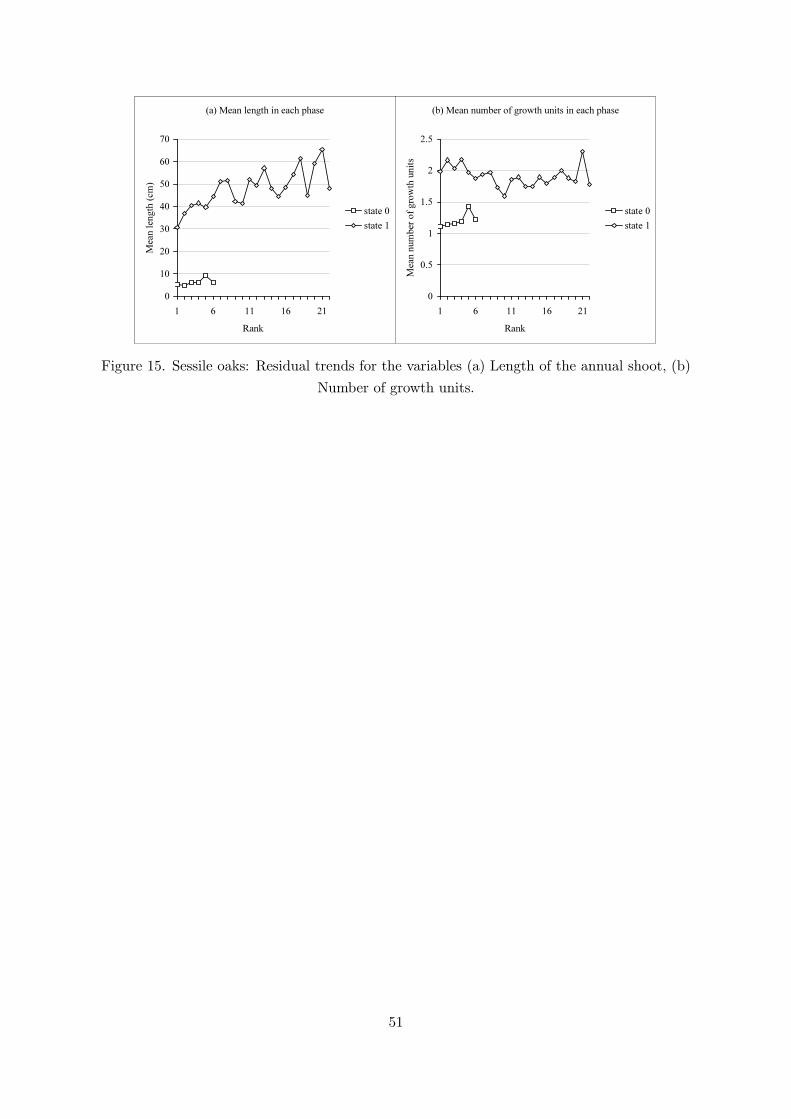
(a) Mean length in each phase

010203040506070

1 6 11 16 21Rank

Mean

leng

th (cm

)

state 0state 1

(b) Mean number of growth units in each phase

0

0.5

1

1.5

2

2.5

1 6 11 16 21Rank

Mean

numb

er of

growt

h unit

s

state 0state 1

(a) Mean length in each phase

010203040506070

1 6 11 16 21Rank

Mean

leng

th (cm

)

state 0state 1

(b) Mean number of growth units in each phase

0

0.5

1

1.5

2

2.5

1 6 11 16 21Rank

Mean

numb

er of

growt

h unit

s

state 0state 1

Figure 15. Sessile oaks: Residual trends for the variables (a) Length of the annual shoot, (b)Number of growth units.

51

0

0.1

0.2

0.3

0.4

0.5

0.6

0.7

0.8

0.9

1

0 10 20 30 40 50 60 70 80 90 100 110 120 130 140 150Shoot length (cm)

Cumu

lative

distr

ibutio

n fun

ction

datamixture

0

5

10

15

20

25

0 10 20 30 40 50 60 70 80 90 100 110 120 130 140 150Shoot length (cm)

Frequ

ency data

state 0, NB(1, 2.7, 0.34)state 1, NB(0, 3.8, 0.08)mixture

0

0.1

0.2

0.3

0.4

0.5

0.6

0.7

0.8

0.9

1

0 10 20 30 40 50 60 70 80 90 100 110 120 130 140 150Shoot length (cm)

Cumu

lative

distr

ibutio

n fun

ction

datamixture

0

5

10

15

20

25

0 10 20 30 40 50 60 70 80 90 100 110 120 130 140 150Shoot length (cm)

Frequ

ency data

state 0, NB(1, 2.7, 0.34)state 1, NB(0, 3.8, 0.08)mixture

Figure 16. Sessile oaks, two-state hidden semi-Markov chain: Mixture of observationdistributions for the “length of the annual shoot” variable.

52

0

0.1

0.2

0.3

0.4

0.5

0.6

0 1 2 3 4 5 6 7 8Sojourn time

Probabil

ity

NB(1, 1, 0.6)NB(1, 6.1, 0.89)

0

0.1

0.2

0.3

0.4

0 5 10 15Sojourn time

Probabil

ity

NB(1, 1, 0.36)NB(1, 1.12, 0.4)

0

0.1

0.2

0.3

0.4

0.5

0.6

0 1 2 3 4 5 6 7 8Sojourn time

Probabil

ity

NB(1, 1, 0.6)NB(1, 6.1, 0.89)

0

0.1

0.2

0.3

0.4

0 5 10 15Sojourn time

Probabil

ity

NB(1, 1, 0.36)NB(1, 1.12, 0.4)

Figure 17. Sessile oaks: Occupancy distributions for the two semi-Markovian and Markovianrecurrent states: (a) state 1, (b) state 2.

B(1, 7, 0.53)

0

0.2

0.4

0 2 4 6

1 20

0.63 0.3 0.07

0.640.4

0.6

0.36

B(1, 7, 0.53)

0

0.2

0.4

0 2 4 6

1 20

0.63 0.3 0.07

0.640.4

0.6

0.36

B(1, 7, 0.53)

0

0.2

0.4

0 2 4 6

1 20 11 220

0.63 0.3 0.07

0.640.4

0.6

0.36

Figure 18. Sessile oaks: Estimated underlying hybrid Markov/semi-Markov chain. Each stateis represented by a vertex which is numbered. The vertex representing the transient state is

edged by a single line while the vertices representing the recurrent states are edged by a doubleline. The possible transitions between states are represented by arcs with the attachedprobabilities noted nearby when < 1. Arcs entering in states indicate initial states. The

attached initial probabilities are noted nearby. The occupancy distribution of thesemi-Markovian state 0 is figured above the corresponding vertex.

53

0

0.1

0.2

0.3

0.4

0.5

0.6

0.7

0.8

0.9

1

0 10 20 30 40 50 60 70 80 90 100 110 120 130 140Shoot length (cm)

Cumu

lative

distr

ibutio

n fun

ction

datamixture

0

5

10

15

20

25

0 10 20 30 40 50 60 70 80 90 100 110 120 130 140Shoot length (cm)

Frequ

ency

datastate 0, NB(1, 3.2, 0.39)state 1, NB(0, 5.1, 0.17)state 2, NB(12, 5.6, 0.11)mixture

0

0.1

0.2

0.3

0.4

0.5

0.6

0.7

0.8

0.9

1

0 10 20 30 40 50 60 70 80 90 100 110 120 130 140Shoot length (cm)

Cumu

lative

distr

ibutio

n fun

ction

datamixture

0

5

10

15

20

25

0 10 20 30 40 50 60 70 80 90 100 110 120 130 140Shoot length (cm)

Frequ

ency

datastate 0, NB(1, 3.2, 0.39)state 1, NB(0, 5.1, 0.17)state 2, NB(12, 5.6, 0.11)mixture

Figure 19. Sessile oaks, three-state hidden hybrid Markov/semi-Markov chain: Mixture ofobservation distributions for the “length of the annual shoot” variable.

54

0

20

40

60

80

100

120

140

160

180

0 10 20 30 40 50 60 70 80 90 100 110 120 130 140 150Internode rank

Leng

th (m

m) dataMeanMean-varianceVariance

Figure 20. Dicorynia guianensis: Segmentation with three change-point models.

55