Analyzing Floods: Understanding Past Flood Events … · Analyzing Floods: Understanding Past Flood Events and Considering ... W.11-12.1 Write arguments to support claims in an analysis

Version 2-published January 2015 Page 1 of 20 View Creative Commons Attribution 4.0 Unported License at http://creativecommons.org/licenses/by/4.0/. Educators may use or adapt.

Analyzing Floods: Understanding Past Flood Events and Considering

Future Flood Events in a Changing Climate —

High School Sample Classroom Task

Introduction

In the first half of 1993, a “perfect storm” of climatic and weather events sent a record amount of water

flooding through the Upper Mississippi River Drainage Basin. Climate models predict that as the global

climate changes, it is likely that there will be larger and more frequent storms, which will lead to larger

flood events like the flood of 1993. In this task, students use recurrence intervals from the Mississippi

River to estimate the expected size and frequency of 100-year and 500-year floods for historical data

(1943 to 1992) and an imaginary future scenario where large floods are more frequent (1943 to 2021).

They compare the recurrence interval versus discharge on semi-log scatterplots and consider data from

global climate models to make evidence based-claims about how changing climate in a warming world

will influence river discharge and flood events. This task is adapted from:

McConnell, D., Steer, D., Knight, C., Owens, K., & Park, L. (2008). The good earth: Introduction to

earth Science, p. 536. New York: McGraw Hill Higher Education.

Hirabayashi, Y., Mahendran, R., Koirala, S., Konoshima, L., Yamazaki, D., Watanabe, S., Kim, H., and

Kanae, S. (2013). Global flood risk under climate change. Nature Climate Change, 3, 816–821. The Weather Channel. The Mississippi River Flood of 1993. Available at:

www.weather.com/encyclopedia/flood/miss93.html. Last accessed: October 18, 2013.

Standards Bundle

(Standards completely highlighted in bold are fully addressed by the task; where all parts of the standard are not addressed by the task,

bolding represents the parts addressed.)

CCSS-M

MP.2 Reason abstractly and quantitatively.

MP.3 Construct viable arguments and critique reasoning of others.

MP.4 Model with mathematics.

HSN.Q.A.1 Use units as a way to understand problems and to guide the solution of multi-step

problems; choose and interpret units consistently in formulas; choose and interpret

scale and the origin in graphs and data displays.

HSN.Q.A.3 Choose a level of accuracy appropriate to limitations on measurement when

reporting quantities.

HSS.ID.B.6 Represent data on two quantitative variables on a scatter plot, and describe how

the variables are related.

HSS.ID.B.6a (Algebra 2 Option) Fit a function to the data; use functions fitted to data to solve

problems in the context of the data.

HSF.IF.C.7e (Algebra 2 Option) Graph exponential and logarithmic functions, showing

intercepts and end behavior, and trigonometric functions, showing period, midline,

http://www.weather.com/encyclopedia/flood/miss93.html

http://www.google.com/url?q=http%3A%2F%2Fwww.corestandards.org%2Fmath%2Fpractice&sa=D&sntz=1&usg=AFQjCNG_CwTEQAmO4n-96gittLPtet1jxA

http://www.corestandards.org/Math/Content/HSF/IF/C/7/e


and amplitude.

HSA.CED.2a (Algebra 2 Option) Create equations in two or more variables to represent

relationships between quantities; graph equations on coordinate axes with labels

and scales.

NGSS

HS-ESS2-2 Analyze geoscience data to make the claim that one change to Earth’s surface

can create feedbacks that cause changes to other Earth systems.

HS-ESS3-1 Construct an explanation based on evidence for how the availability of natural

resources, occurrence of natural hazards, and changes in climate have influenced

human activity.

HS-ESS3-5 Analyze geoscience data and the results from global climate models to make an

evidence-based forecast of the current rate of global or regional climate change

and associated future impacts to Earth systems.

CCSS-ELA/Literacy

W.11-12.1 Write arguments to support claims in an analysis of substantive topics or texts,

using valid reasoning and relevant and sufficient evidence. WHST.11-12.1 Write arguments focused on discipline-specific content.

W.11-12.1.a and WHST.11-12.1.a

Introduce precise, knowledgeable claim(s), establish the significance of the

claim(s), distinguish the claim(s) from alternate or opposing claims, and create an

organization that logically sequences claim(s), counterclaims, reasons, and

evidence. W.11-12.1.b Develop claim(s) and counterclaims fairly and thoroughly, supplying the most

relevant evidence for each while pointing out the strengths and limitations of both

in a manner that anticipates the audience's knowledge level, concerns, values, and

possible biases. WHST.11-12.1.b Develop claim(s) and counterclaims fairly and thoroughly, supplying the most

relevant data and evidence for each while pointing out the strengths and

limitations of both claim(s) and counterclaims in a discipline-appropriate form that

anticipates the audience's knowledge level, concerns, values, and possible biases.

Information for Classroom Use

Connections to Instruction This task is aimed at students who have taken Algebra 1, but it includes additional options that expand

the plotting components for students who have taken Algebra 2. This task could fit within an

instructional unit on rivers, natural hazards, and/or climate change. Task Components A and C,

including the additional options, would fit well within an Algebra 2 course as a real-world example of

logarithmic relationships.

Overall, the entire task can be used in a unit when students have strong command of the plotting

components and the science content underpinning the task, as listed in the assumptions. Task

Components A through E could be used as a check for understanding, or formative assessment, with of

the math and science concepts included in the task. Because the plotting tasks are similar, Task

http://www.corestandards.org/ELA-Literacy/W/11-12/1/b/

http://www.corestandards.org/ELA-Literacy/WHST/11-12/1/b/


Component A could be used as a formative assessment followed by Task Component C as a subsequent

check for understanding of the plotting components.

Because this task requires students to use evidence and reasoning to make, support, and evaluate

forecasts, it can be used to check for understanding claims in writing argument in ELA/Literacy.

Students can be formatively assessed on writing argument in Task Components B, D, and E. The option

for Task Component A also allows a check for understanding in writing argument. This task has been

aligned to the ELA/Literacy standards for writing argument for the 11–12 grade band.

Teachers using this task in 9th or 10th grade should refer to the comparable CCSS for the 9–10

grade band.

Approximate Duration for the Task The entire task likely will take 3–6 class periods (45–50 minutes each) spread out over the course of an

instructional unit, with the divisions listed below: Task Component A: 1–2 class periods Task Component B: 1–2 class periods, depending on whether done as homework Task Component C: 1–2 class periods Task Component D: 1–2 class periods, depending on whether done as homework Task Component E: up to 1 class period

Note that this timeline only refers to the approximate time a student may spend engaging in the task

components, and does not reflect any instructional time that may be interwoven with this task.

Assumptions To effectively complete the task, instructors and students should have a working understanding of

stream discharge, the factors that affect flooding, what is meant by a 100-year and 500-year storms, the

concept of recurrence intervals for floods, the basics of global climate change, and how to use a semi-

log graph to plot and interpret logarithmic data. Materials Needed All materials needed to complete this task are provided as attachments. If the teacher decides to allow

students to use a spreadsheet/plotting program or graphing calculators, then the students need access to

such programs and need to understand how to use them. Although not necessary to complete the task,

teachers may choose to read about or include alternative or additional data from the article by

Hirabayashi et al. (2013), in which case teachers would need access to the article (cited in the

introduction) in the journal Nature Climate Change.

Supplementary Resources ● Teaching the Quantitative Concepts in Floods and Flooding by Dr. Eric Baer:

http://serc.carleton.edu/quantskills/methods/quantlit/floods.html. This resource outlines

concepts that students typically struggle with and has many examples and explanations. ● Additional information about the 1993 Mississippi River flood can be found at Prof. Charles L.

Smart’s website: www.kean.edu/~csmart/Observing/13.%20Streams%20and%20floods.pdf

● Information about rivers and flooding can be reviewed through Science Courseware’s Virtual

River Flooding, found at Geology Labs On-line: www.sciencecourseware.org/VirtualRiver.

Accommodations for Classroom Tasks

To accurately measure three dimensional learning of the NGSS along with CCSS for

mathematics, modifications and/or accommodations should be provided during instruction and

assessment for students with disabilities, English language learners, and students who are speakers of

http://serc.carleton.edu/quantskills/methods/quantlit/floods.html

http://www.kean.edu/~csmart/Observing/13.%20Streams%20and%20floods.pdf

http://www.sciencecourseware.org/VirtualRiver


social or regional varieties of English that are generally referred to as “non-Standard English”.

Classroom Task

Context In the first half of 1993, a perfect storm of climatic and weather events sent a record amount of water

flooding through the Upper Mississippi River Drainage Basin. From January through July of that year,

record amounts of snow fell on several upper Midwest states. Second, heavy storms added large

amounts of rainfall all at once in parts of the basin. This higher-than-normal precipitation filled storage

reservoirs and saturated the ground, leading to the spatially largest flood in U.S. history, one that

covered 44,000 square kilometers (17,000 square miles) in nine states (McConnell et al., p. 310). Over

70,000 people were displaced by the floods. Nearly 50,000 homes were damaged or destroyed, and 52

people died. More than 12,000 square miles of productive farmland were rendered useless. Damage

costs were estimated between $15 billion and $20 billion (The Weather Channel). Scientists compare floods like the one that occurred on the Mississippi River in 1993 with other floods

that occurred on the same river in other years by calculating the flood’s recurrence interval over a

specific period of time in the past. First, the flood events that occurred in a specific time range are

ranked in order of greatest to least discharge (i.e., the amount of water flowing in the stream at any

given second). For each flood event, the rank is used to calculate recurrence interval: RI = (N+1)/rank,

where N = the total number of years within the chosen time range. The recurrence interval (calculated

from past events) is used to gauge the future probability of an event by calculating the percent chance

that a similar flood will occur again in any given year (Baer, SERC website). The percent probability

(P) of an event with recurrence interval (RI) is P = (1/RI)*100. When the recurrence interval is plotted

on a semi-log scatterplot with discharge, the logarithmic trend line (line of best fit) can be used to

predict the probability of a flood of any discharge occurring in a given year, including the 100-year and

500-year flood values used on building flood zone maps. (Note: Because of the abundance of data

points with low RI values, trendlines may be more easily calculated with datasets that exclude RI values

less than 2.)


The trend line (line of best fit) on the semi-log scatterplot of recurrence interval versus the amount of flood water

(a stream’s discharge) like the one above can be used to predict the size of floods during 100-year (recurrence

interval of 100) and 500-year flood events (recurrence interval of 500). Image is derived from:

http://web.mst.edu/~rogersda/umrcourses/ge301/what%20is%20a%20100%20year%20flood.htm

Last accessed: February 8, 2014

Climate models predict that as the global climate changes, weather patterns also will change. In some

areas, it is likely that there will be larger and more frequent storms and unusual weather conditions like

those that led to the flood of 1993. This has implications for what we understand the discharge of a

100-year storm to be. Because the RI is calculated from the flood data over a specific time range, a

dataset with a larger number of severe flood events could change the recurrence intervals, the trend line

(line of best fit) on the scatterplot, and the predicted size of the 100-year and 500-year floods. In this task, you will use streamflow data from the Mississippi River spanning the years from 1943 to

1992 to calculate the recurrence interval for each ranked flood event and the percent chance of the flood

happening in a given year. You will plot that data on a semi-log graph to determine the recurrence

interval of a flood the size of the 1993 flood and make predictions about the size of a 100-year and 500-

year flood. You will then consider the effect that the 1993 flood and seven very large, imaginary flood

events occurring in the near future (up to 2021) will have on the calculated data and flood predictions.

Finally, you will review results from global climate models that make the same type of comparison

between past flooding conditions and future projections of flooding around the world.

Task Components

A. Calculate the recurrence interval and percent probability for flood events on the Mississippi

River at Keokuk, IA, for the time range of 1941–92, a 49-year range (Attachment 1). This

dataset ends the year prior to the 1993 Mississippi River flood and represents historical data

(McConnell et al., p. 313). Plot the discharge versus recurrence interval (RI) on the semi-log


grid provided in Attachment 3. Draw a straight line through the plotted points with RI values of

2 or more and use that line to estimate the size of 100-year and 500-year floods for this river

measuring station at Keokuk (McConnell et al., p. 313). Describe why your graphical

representation of the flood events can be used to estimate the size of 100-year and 500-year

floods for this measuring station.

Additional Option for Students Taking Algebra 2:

In addition to plotting the discharge versus RI on the semi-log grid provided, plot the discharge

versus RI on traditional graph paper and use that equation to calculate the 100-year and 500-

year flood values. Calculate the trendline (line of best fit) equation for each scatterplot either

using paper and pencil calculations or using graphing technology, such as a spreadsheet

program or a graphing calculator. Compare and contrast the equations that were calculated.

Consider whether one scatterplot is more accurate or easier to calculate. Using your

scatterplots as evidence, construct an argument for which, if either, scatterplot allows for

easier estimation of the size of floods for this river.

B. The amount of discharge of a 100-year flood is used by the public to predict whether a home is

at risk of flooding (i.e., within the area affected by a 100-year flood) or not at risk of flooding

(i.e., outside of the area affected by a 100-year flood). The discharge of the 1993 Mississippi

flood at Keokuk, IA, was 446,000 cubic feet/second. Consider the recurrence interval and

percent probability of the 1993 flood. Using observations based on your scatterplot, construct

an argument for how this natural hazard event is likely to have changed how homeowners

decide whether their homes are in danger of flood damage and where builders may decide to

construct new homes in the future.

C. Attachment 2 imagines a future where large floods like the 1993 flood on the Mississippi River

are more common. Calculate the recurrence interval and percent probability for the past flood

events and the seven imaginary future flooding events on the Mississippi River at Keokuk,

Iowa for the time range of 1941-2021, an 80-year time range (Attachment 1). Plot the discharge

versus recurrence interval (RI) on the semi-log grid provided. Draw a straight line through the

plotted points with RI values of 2 or more and use that line to estimate the new size of 100-year

and 500-year floods in this imaginary future scenario. Describe why this this line can be used to

estimate the 100- and 500-year floods in the future scenario.

Additional Option for Students Taking Algebra 2: Determine an equation for the future trend line (line of best fit) and use that equation to

calculate the 100-year and 500-year flood values. On one semi-log graph, plot the equations

for both of the trend lines, and consider the differences between the current trend (from Task

Component A) and the possible future trend (from Task Component C). Student also will use

this scatterplot for Task Component D.

D. Compare the historical and future semi-log scatterplots and use your observations of the data

and trend lines to create an evidence-based prediction for the effect a changing climate could

have on the size and frequency of flooding events on Mississippi River at Keokuk, IA, if

weather conditions like those that lead to the 1993 become more common. As part of your

forecast, make a claim about the rate of climate change in this imaginary future scenario.

Describe how the evidence supports your forecast.

E. Climate scientists used historical flood data to calculate the current predicted 100-year flood


discharge values for areas all around the world just like you did in Task Component A. They

also created global climate models to imagine where flood events are most likely to happen,

how large they would be and how often they might occur in the next 100 years as the climate

warms. They use these models to calculate a future 100-year discharge value just like you did

in Task Component C. Scientists compared the historic and future world 100-year flood data

values as you did when you compared your two scatterplots, and the results of the comparison

model are shown in Attachment 4.

Use the model results to make an evidence-based forecast about the effects a changing climate

could have on the size and frequency of flooding events in different parts of the world. As part

of your forecast, make a statement about the rate of climate change predicted by the model

(considering the time range chosen for the calculations). Describe how the evidence supports

your forecast. In your description, compare your global forecast to the forecast you made for

the Mississippi River (considering types of effects and the rate of climate change), and discuss

which is more useful in predicting the effects of climate change: data from a single area

somewhere in the world (regional data) or global model results.


Alignment and Connections of Task Components to the Standards Bundle

Task Components A and C ask students to calculate flood recurrence interval values for historical

annual peak discharge data and for annual peak discharge data of a potential future time range, to plot

these data on a semi-log scatterplot, and to estimate the size of 100-year and 500-year floods for

historical and future data. Together these partially address parts (individual practice bullets from

Appendix F) of the NGSS practices of Analyzing and Interpreting Data and Using Mathematics

and Computational Thinking; parts (bullets from Appendix G) of the NGSS crosscutting concepts of

Stability and Change and Patterns; and the CCSS-M practices MP.2 and MP.4. By plotting values

on a semi-log scatterplot, students can check their understanding of parts of the CCSS-M content

standard of HSS.ID.6, and by using those scatterplots to estimate the size of a 100-year and 500-year

flood, the students can partially address the CCSS-M content standards of HSN.Q.A.1 and HSN.Q.A.3.

Plotting and interpreting data in these task components enhance performances involving the science

practices and crosscutting concepts, whereas the scientific context of modeling discharge events

enhances assessment of the math standards. In the Additional Option for Students Taking Algebra 2,

students are asked to determine trend line (line of best fit) equations for the data and to compare the

data on a semi-log scatterplot with a regular scatterplot, which partially addresses the CCSS-M

standards of HSA.CED.2 and HSS.ID.B.6a. The advanced option also asks students to plot the trend

line equations on a semi-log scatterplot, which partially addresses the CCSS-M standard of

HSF.IF.C7.e. Task Component B asks students to use the scatterplot they made for the historical data as evidence to

construct an explanation for how the 1993 flooding event affected human behavior. This partially

addresses the NGSS performance expectation HS-ESS3-1 by partially addressing parts (bullets from

Appendix E) of the associated disciplinary core idea of Natural Hazards (ESS3.B as it relates to HS-

ESS3-1) and part of the associated crosscutting concept Cause and Effect. The task requires the

students to consider where the 1993 flood fits within the historical data when making their explanation,

which partially addresses parts of the NGSS practices of Engaging in Argument from Evidence and

Analyzing and Interpreting Data, Using Mathematical and Computational Thinking, and the

CCSS-M practices of MP.1 and MP.3. By requiring students to use their observations and reasoning to

construct an evidence-based scenario, this task partially addresses the ELA/ Literacy standards W.11-

12.1, W.11-12.1.a, WHST.11-12.1, and WHST.11-12.1.a, writing argument. Task Component D asks students to make an evidence-based forecast for how a changing climate will

affect river systems like the Mississippi River. This partially addresses the NGSS performance

expectation of HS-ESS2-2 by partially addressing parts of the practice of Analyzing and Interpreting

Data (as it relates to HS-ESS2-2) and the disciplinary core idea of Weather and Climate (ESS2.D as

it relates to HS-ESS2-2). This also partially addresses parts of the NGSS crosscutting concepts of

Stability and Change and Cause and Effect. By using information from data tables and semi-log

scatterplots as evidence to support their claim, students can demonstrate their understanding of parts of

the NGSS practices of Using Mathematical and Computational Thinking and Engaging in

Argument from Evidence and the CCSS-M practices of MP.1 and MP.3. By asking students to

compare scatter plots and use their observations to construct an evidence-based forecast and support

their claim, this task partially addresses the ELA/ Literacy standards W.11-12.1, W.11-12.1.a, W.11-

12.1.b, WHST.11-12.1, WHST.11-12.1.a, and WHST.11-12.1.b, writing argument.

Task Component E asks students to interpret climate model results to make an evidence-based

forecast about the effects climate change will have on river discharge around the world and to compare

this forecast with the local forecast they made for the Mississippi River using the data plots, including a

http://www.corestandards.org/Math/Content/HSN/Q

http://www.corestandards.org/Math/Content/HSN/Q


comparison of the rate of climate change. This partially assesses the NGSS performance expectation of

HS-ESS3-5 by partially assessing part of the associated practice of Analyzing and Interpreting Data

(as it relates to HS-ESS3-5), part of the disciplinary core idea of Global Climate Change (ESS3.D as

it relates to HS-ESS3-5), and part of the crosscutting concept of Stability and Change (as it relates

to HS-ESS3-5). This also partially assesses parts of the NGSS crosscutting concepts of Scale,

Proportion, and Quantity and Cause and Effect; parts of the NGSS practices of Developing and

Using Models, Analyzing and Interpreting Data, and Engaging in Argument from Evidence; and

the CCSS-M practices of MP.1 and MP.3. By requiring students to use model results to construct and

support an evidence-based forecast and make informed statements and comparisons about forecasts,

this task partially assesses the ELA/ Literacy standards W.11-12.1, W.11-12.1.a, W.11-12.1.b,

WHST.11-12.1, WHST.11-12.1.a, and WHST.11-12.1.d, writing argument. Together, Task Components A, C, D and E partially address the NGSS performance expectation of

HS-ESS3-5. Through the use of graphical displays of flood data, the interpretation of patterns in the

frequency and size of flood events, and development of forecasts for the effect of climate change on

flood events using data and model results, the task components are addressing part of the disciplinary

core idea of ESS3.D: Global Climate Change, and part of the crosscutting concept of Stability and

Change through part of the practice of Analyzing and Interpreting Data (as they relate to this

performance expectation). By comparing the forecasts (derived from the data), including a

comparison of rates of climate change and the types of change in flood size and frequency, and by

considering the effectiveness of regional data versus climate models in understanding the effects of

climate change, students completing the task components are integrating the disciplinary core ideas

with the crosscutting concepts and the practices.

Evidence Statements

Task Component A ● Students calculate the recurrence interval and percent probability for the historic flood events

on the Mississippi River.

● Students plot the historic discharge and recurrence interval data on the semi-log graph, and

draw an increasing, straight trend line (line of best fit) through the data points. ● Students use the trend line to estimate the discharge amount for 100-year and 500-year flood

events for the historic data.

● Students describe that the mathematical representations of the discharge and recurrence interval

illustrate a pattern of change, which allowed them to estimate the value at the measuring

station.

● Additional Option for Students Taking Algebra 2 (includes all of the following): ○ Students plot the historic discharge and recurrence interval data on the traditional

graph paper (non-log scatterplot), and draw a nonlinear trend line (line of best fit)

through the data points. ○ Students derive an equation that models the nonlinear trend line on the non-log

scatterplot.

○ Students derive an equation that models the straight trend line (line of best fit) on the

semi-log plot. ○ Students use the trend line equation(s) to calculate discharge amounts for the 100-year

and 500-year floods.

○ Students construct an argument, including a claim as to which scatterplot (non-log


versus semi-log) allows for easier estimation of the size of floods for this river ○ Students identify and describe interpretations of the scatterplots as evidence for the

claim. ○ In their argument, students include a line of reasoning that compares the data

presentation and equations of the two scatterplots

○ In their argument, students evaluate the data presentation and equations of the two

scatterplots for their relevance and sufficiency to support their claim. Task Component B

● Students use the trend line to estimate the recurrence interval and percent probability for a

flood with discharge of 446,000 cubic feet/second. ● Students make a specific claim or claims for how the 1993 flood is likely to have had effects on

how homeowners and builders make decisions regarding 1) whether existing homes are in

danger, and 2) where new buildings should be constructed in the future. ● In support of their claim, students identify and describe evidence from the scatterplots,

including that the 1993 flood had a greater discharge than the historic 100-year flood.

● Students describe the utility of the historical 100-year flood map in predicting flood damage

given the 1993 flood ● Students evaluate the utility of both the historical 100-year flood map and the 1993 flood data

in determining flood risk ● Students make a connection between the size of the flood and the area of land affected by the

flood (i.e., the larger the discharge value, the greater the area of land affected)

● Students synthesize the evidence and evaluation to argue, with logical reasoning, that the 1993

flood likely changed homeowners’ and builders’ attitudes towards using the historical 100-year

map for predicting damage likelihood and building sites. Task Component C

● Students calculate the new recurrence interval and percent probability for the past and

imaginary flood events on the Mississippi River.

● Students plot the “future” discharge and recurrence interval data on the semi-log graph, and

draw an increasing, straight trend line (line of best fit) through the data points. ● Students use the trendline to estimate the discharge amount for 100-year and 500-year flood

events for the future data.

● Students use algebraic thinking to describe why the trendline predicts the discharge amount for

the future data. ● Additional Option for Students Taking Algebra 2 (includes all of the following):

○ Students derive an equation that models the straight trend line (line of best fit) on the

semi-log plot. ○ Students use the future trend line equation to calculate discharge amounts for the 100-

year and 500-year floods.

○ Students plot the historic and future trend line equations on one semi-log graph. Task Component D

● Students create a forecast that makes a prediction for how the size (discharge) and frequency

(recurrence interval) of flood events along the Mississippi River will change in response to a

changing climate. ● In their forecast, students include a statement about the rate of climate change in the imaginary

future scenario that relates the rate to those observed in the scatterplots.


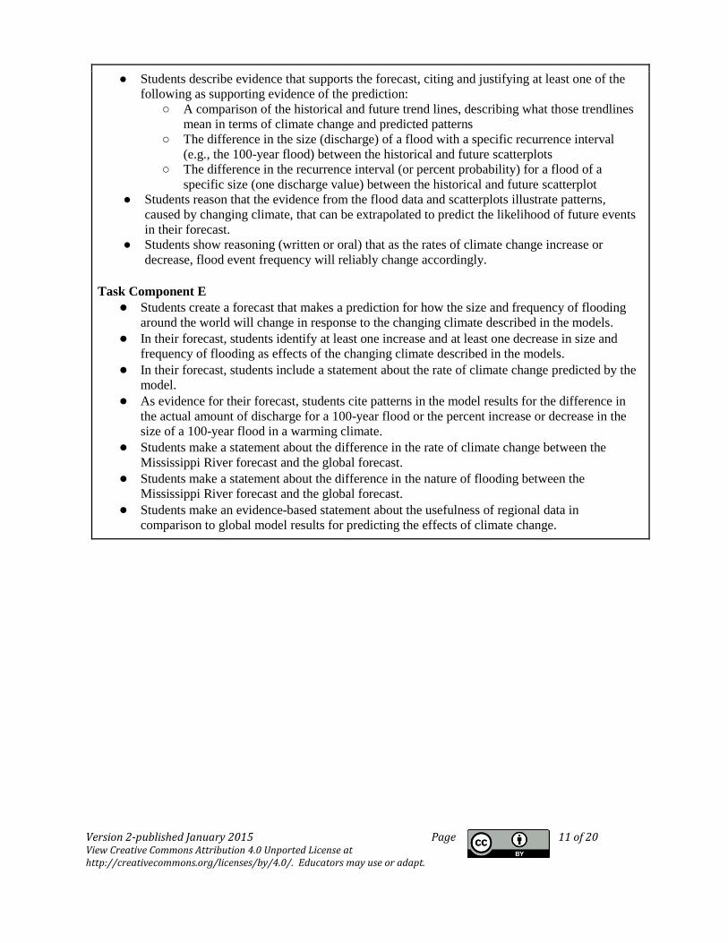
● Students describe evidence that supports the forecast, citing and justifying at least one of the

following as supporting evidence of the prediction:

○ A comparison of the historical and future trend lines, describing what those trendlines

mean in terms of climate change and predicted patterns

○ The difference in the size (discharge) of a flood with a specific recurrence interval

(e.g., the 100-year flood) between the historical and future scatterplots

○ The difference in the recurrence interval (or percent probability) for a flood of a

specific size (one discharge value) between the historical and future scatterplot

● Students reason that the evidence from the flood data and scatterplots illustrate patterns,

caused by changing climate, that can be extrapolated to predict the likelihood of future events

in their forecast.

● Students show reasoning (written or oral) that as the rates of climate change increase or

decrease, flood event frequency will reliably change accordingly.

Task Component E

● Students create a forecast that makes a prediction for how the size and frequency of flooding

around the world will change in response to the changing climate described in the models. ● In their forecast, students identify at least one increase and at least one decrease in size and

frequency of flooding as effects of the changing climate described in the models.

● In their forecast, students include a statement about the rate of climate change predicted by the

model. ● As evidence for their forecast, students cite patterns in the model results for the difference in

the actual amount of discharge for a 100-year flood or the percent increase or decrease in the

size of a 100-year flood in a warming climate. ● Students make a statement about the difference in the rate of climate change between the

Mississippi River forecast and the global forecast. ● Students make a statement about the difference in the nature of flooding between the

Mississippi River forecast and the global forecast.

● Students make an evidence-based statement about the usefulness of regional data in

comparison to global model results for predicting the effects of climate change.


Attachment 1. Historical Flood Data Chart

RI = (N+1)/rank, where N = number of years; P = (1/RI)*100

Rank Year Discharge (ft3/s) Recurrence

Interval (RI) % probability (P) of a flood of this magnitude

occurring within any given year

1 1973 344,000 50 2.00

2 1965 327,000 25 4.00

3 1960 289,500 17 5.99

4 1986 268,000

5 1951 265,100

6 1974 260,000

7 1979 257,000

8 1944 256,000

9 1952 253,800

10 1969 253,000

11 1975 252,000

12 1947 245,700

13 1986 241,000

14 1948 233,600

15 1982 225,000

16 1962 224,100

17 1983 224,000

18 1946 223,300

19 1967 221,200

20 1976 214,000

25 1972 192,000

30 1954 181,400

40 1970 140,000

49 1977 79,800


Attachment 2. Hypothetical Future Flood Data Chart .

Rank Year Discharge

(ft3/s) Recurrence

Interval (RI) % probability of a flood of

this magnitude occurring

within any given year

1 1993 446,000 81.0 1.2

2 Future Severe Storm 400,600 40.5 2.5

3 Future Severe Storm 369,000 27.0 3.7

4 Future Severe Storm 351,000

5 1973 344,000

6 1965 327,000




10 1960 289,500


12 1986 268,000

13 1951 265,100

14 1974 260,000

15 1979 257,000

16 1944 256,000

17 1952 253,800

18 1969 253,000

19 1975 252,000

20 1947 245,700

21 1986 241,000

22 1948 233,600


23 1982 225,000

24 1962 224,100

25 1983 224,000

26 1946 223,300

27 1967 221,200

28 1976 214,000

30 1972 192,000

48 1954 181,400

49 1970 140,000

78 1977 79,800


Attachment 3. Semi-log Graph Note: Teachers may choose to have their students design their own plots rather than be given the plot below.


Attachment 4. Global Climate

Model Results

Model results show:

(a) the amount of discharge

(mm/day) associated with a 100-year

flood for historical data (1971–

2000), and

(b) the amount of discharge

(mm/day) associated with a 100-year

flood for future model data (2071–

2100).

Comparison of the two models show:

(c) the difference in the actual

amount of discharge for a 100-year

flood (mm/day), and

(d) the percent increase or decrease

in the size of a 100-year flood in a

warming climate.

This image is Figure S4 from the

supplementary material for the

following paper: Hirabayashi, Y., Mahendran, R.,

Koirala, S., Konoshima, L.,

Yamazaki, D., Watanabe, S., Kim,

H., and Kanae, S. (2013). Global

flood risk under climate change.

Nature Climate Change, 3, 816–821. The image is used with permission

from the authors.


Attachment 5. Graphs for Additional Option for Students Taking Algebra 2


Note: Teachers may choose to have their students design their own plots rather than be given the plot.


Note: Teachers may choose to have their students design their own plots rather than be given the plot.

Sample Answer Scatterplots


Documents

Analyzing Floods: Understanding Past Flood Events … · Analyzing Floods: Understanding Past Flood Events and Considering ... W.11-12.1 Write arguments to support claims in an analysis