Analyzing Designs with Quartus II Netlist Viewers, Quartus ... · The Quartus II RTL Viewer displays a sc hematic view of the design netlist after Analysis and Elaboration or netlist

Altera Corporation 12–1May 2008

12. Analyzing Designs withQuartus II Netlist Viewers

Introduction As FPGA designs grow in size and complexity, the ability to analyze how your synthesis tool interprets your design becomes critical. Often, with today’s advanced designs, several design engineers are involved in coding and synthesizing different design blocks, making it difficult to analyze and debug the design. The Quartus® II RTL Viewer, State Machine Viewer, and Technology Map Viewer provide powerful ways to view your initial and fully mapped synthesis results during the debugging, optimization, or constraint entry process.

The first section in this chapter, “When to Use Viewers: Analyzing Design Problems”, describes examples of using the viewers to analyze your design at various stages of the design cycle. The sections following this provide an introduction to the Quartus II design flow using netlist viewers, an overview of each viewer, and an explanation of the user interface. These sections describe the following tasks:

■ How to navigate and filter schematics■ How to probe to and from other windows within the Quartus II

software■ How to view a timing path from the Timing Analyzer report

This chapter contains the following sections regarding netlist viewers:

■ “Introduction to the User Interface” on page 12–7■ “Navigating the Schematic View” on page 12–21■ “Filtering in the Schematic View” on page 12–36■ “Probing to Source Design File and Other Quartus II Windows” on

page 12–44■ “Probing to the Viewers from Other Quartus II Windows” on

page 12–46■ “Viewing a Timing Path” on page 12–47■ “Other Features in the Schematic Viewer” on page 12–49■ “Debugging HDL Code with the State Machine Viewer” on

page 12–58

The final section, provides a detailed example that uses the viewer to analyze a design and quickly resolve a design problem.

QII51013-8.0.0

12–2 Altera CorporationMay 2008

Quartus II Handbook, Volume 1

When to Use Viewers: Analyzing Design Problems

You can use netlist viewers to analyze your design to determine how it was interpreted by the Quartus II software. This section provides simple examples of how to use the RTL viewers, State Machine, and Technology Map Viewers to analyze problems encountered in the design process.

The following sections contain information about how netlist viewers display your design:

■ “Quartus II Design Flow with Netlist Viewers”■ “RTL Viewer Overview”■ “State Machine Viewer Overview”■ “Technology Map Viewer Overview”

Using the RTL Viewer is a good way to view your initial synthesis results to determine whether you have created the desired logic, and that the logic and connections have been interpreted correctly by the software. You can use the RTL Viewer and State Machine Viewer to check your design visually before simulation or other verification processes. Catching design errors at this early stage of the design process can save you valuable time.

If you see unexpected behavior during verification, use the RTL Viewer to trace through the netlist and ensure that the connections and logic in your design are as expected. You can also use the State Machine Viewer to view state machine transitions and transition equations. Viewing the design can help you find and analyze the source of design problems. If your design looks correct in the RTL Viewer, you know to focus your analysis on later stages of the design process and investigate potential timing violations or issues in the verification flow itself.

You can use the Technology Map Viewer to look at the results at the end of synthesis and technology mapping by running the viewer after performing Analysis and Synthesis. If you have compiled your design through the Fitter stage, you can view your post-mapping netlist in the Technology Map Viewer (Post-Mapping) and your post-fitting netlist in the Technology Map Viewer. If you perform only Analysis and Synthesis, both viewers display the same post-mapping netlist.

In addition, you can use the RTL Viewer or Technology Map Viewer to locate the source of a particular signal, which can help you debug your design. Use the navigation techniques described in this chapter to search easily through the design. You can trace back from a point of interest to find the source of the signal and ensure the connections are as expected.

You can also use the Technology Map Viewer to help you locate post-synthesis nodes in your netlist and make assignments when optimizing your design. This functionality is useful, for example, when


Quartus II Design Flow with Netlist Viewers

making a multicycle clock timing assignment between two registers in your design. Start at an I/O port and trace forward or backward through the design and through levels of hierarchy to find nodes that interest you, or locate a specific register by visually inspecting the schematic.

You can use the RTL Viewer, State Machine Viewer, and Technology Map Viewer in many other ways throughout the design, debugging, and optimization stages. Viewing the design netlist is a powerful way to analyze design problems. This chapter shows how you can use the various features of the netlist viewers to increase your productivity when analyzing a design.

Quartus II Design Flow with Netlist Viewers

The first time you open one of the netlist viewers after compiling the design, a preprocessor stage runs automatically before the viewer opens. If you close the viewer and open it again later without recompiling the design, the viewer opens immediately without performing the preprocessing stage. Figure 12–1 shows how the netlist viewers fit into the basic Quartus II design flow.

Figure 12–1. Quartus II Design Flow Including the RTL Viewer and Technology Map Viewer



Each viewer requires that your design has been compiled with the minimum compilation stage listed below before the viewer can run the preprocessor and open the design.

■ To open the RTL Viewer or State Machine Viewer, first perform Analysis and Elaboration.

■ To open the Technology Map Viewer or the Technology Map Viewer (Post-Mapping), first perform Analysis and Synthesis.

1 If you open one of the viewers without first compiling the design with the appropriate minimum compilation stage, the viewer does not appear. Instead, the Quartus II software issues an error message instructing you to run the necessary compilation stage and restart the viewer.

Both viewers display the results of the last successful compilation. Therefore, if you make a design change that causes an error during Analysis and Elaboration, you cannot view the netlist for the new design files, but you can still see the results from the last successfully compiled version of the design files. If you receive an error during compilation and you have not yet successfully run the appropriate compilation stage for your project, the viewer cannot be displayed; in this case, the Quartus II software issues an error message when you try to open the viewer.

1 If the viewer window is open when you start a new compilation, the viewer closes automatically. You must open the viewer again to view the new design netlist after compilation completes successfully.

RTL Viewer Overview

The Quartus II RTL Viewer allows you to view a register transfer level (RTL) graphical representation of your Quartus II integrated synthesis results or your third-party netlist file within the Quartus II software.

You can view results after Analysis and Elaboration when your design uses any supported Quartus II design entry method, including Verilog HDL Design Files (.v), SystemVerilog Design Files (.sv), VHDL Design Files (.vhd), AHDL Text Design Files (.tdf), schematic Block Design Files (.bdf), or schematic Graphic Design Files (.gdf) imported from the MAX+PLUS® II software. You can also view the hierarchy of atom primitives (such as device logic cells and I/O ports) when your design uses a synthesis tool to generate a Verilog Quartus Mapping File (.vqm) or Electronic Design Interchange Format (.edf) netlist file. Refer to Figure 12–1 for a flow diagram.


RTL Viewer Overview

The Quartus II RTL Viewer displays a schematic view of the design netlist after Analysis and Elaboration or netlist extraction is performed by the Quartus II software, but before technology mapping and any synthesis or fitter optimization algorithms occur. This view is not the final design structure because optimizations have not yet occurred. This view most closely represents your original source design. If you synthesized your design using the Quartus II integrated synthesis, this view shows how the Quartus II software interpreted your design files. If you are using a third-party synthesis tool, this view shows the netlist written by your synthesis tool.

When displaying your design, the RTL Viewer optimizes the netlist to maximize readability in the following ways:

■ Logic with no fan-out (its outputs are unconnected) and logic with no fan-in (its inputs are unconnected) are removed from the display.

■ Default connections such as VCC and GND are not shown. ■ Pins, nets, wires, module ports, and certain logic are grouped into

buses where appropriate.■ Constant bus connections are grouped.■ Values are displayed in hexadecimal format. ■ NOT gates are converted to bubble inversion symbols in the

schematic.■ Chains of equivalent combinational gates are merged into a single

gate. For example, a 2-input AND gate feeding a 2-input AND gate is converted to a single 3-input AND gate.

■ State machine logic is converted into a state diagram, state transition table, and state encoding table, which are displayed in the State Machine Viewer.

To run the RTL Viewer for a Quartus II project, first analyze the design to generate an RTL netlist. To analyze the design and generate an RTL netlist, on the Processing menu, point to Start and click Start Analysis & Elaboration. You can also perform a full compilation on any process that includes the initial Analysis and Elaboration stage of the Quartus II compilation flow.

To run the viewer, on the Tools menu, point to Netlist Viewers and click RTL Viewer.

You can set the RTL Viewer preprocessing to run during a full compilation, which means you can launch the RTL Viewer after Analysis and Synthesis has completed, but while the Fitter is still running. In this case, you do not have to wait for the Fitter to finish before viewing the schematic. This technique is useful for a large design that requires a substantial amount of time in the place-and-route stage.



To set the RTL Viewer preprocessing to run during compilation, on the Assignments menu, click Settings. In the Category list, select Compilation Process Settings and turn on Run RTL Viewer preprocessing during compilation. By default, this option is turned off.

State Machine Viewer Overview

The State Machine Viewer presents a high-level view of finite state machines in your design. The State Machine Viewer provides a graphical representation of the states and their related transitions, as well as a state transition table that displays the condition equation for each of the state transitions, and encoding information for each state.

To run the State Machine Viewer, on the Tools menu, point to Netlist Viewers and click State Machine Viewer. To open the State Machine Viewer for a particular state machine, double-click the state machine instance in the RTL Viewer or right-click the state machine instance and click Hierarchy Down.

Technology Map Viewer Overview

The Quartus II Technology Map Viewer provides a technology-specific, graphical representation of your design after Analysis and Synthesis or after the Fitter has mapped your design into the target device. The Technology Map Viewer shows the hierarchy of atom primitives (such as device logic cells and I/O ports) in your design. For supported families, you can also view internal registers and look-up tables (LUTs) inside logic cells (LCELLs) and registers in I/O atom primitives. Refer to “Viewing Contents of Atom Primitives” on page 12–22 for details.

1 Where possible, the port names of each hierarchy are maintained throughout synthesis. However, port names may change or be removed from the design. For example, if a port is unconnected or driven by GND or VCC, it is removed during synthesis. When a port name is changed, the port is assigned a related user logic name in the design or a generic port name such as IN1 or OUT1.

You can view your Quartus II technology-mapped results after synthesis, fitting, or timing analysis. To run the Technology Map Viewer for a Quartus II project, on the Processing menu, point to Start and click Start Analysis & Synthesis to synthesize and map the design to the target technology. At this stage, the Technology Map Viewer shows the same post-mapping netlist as does the Technology Map Viewer (Post-Mapping). You can also perform a full compilation, or any process that includes the synthesis stage in the compilation flow.

If you have completed the Fitter stage, the Technology Map Viewer shows the changes made to your netlist by the Fitter, such as physical synthesis optimizations, while the Technology Map Viewer (Post-Mapping) shows


Introduction to the User Interface

the post-mapping netlist. If you have completed the Timing Analysis stage, you can locate timing paths from the Timing Analyzer report in the Technology Map Viewer (refer to “Viewing a Timing Path” on page 12–47 for details). Refer to Figure 12–1 on page 12–3 for a flow diagram.

To run the Technology Map Viewer, on the Tools menu, point to Netlist Viewers and click Technology Map Viewer, or select Technology Map Viewer from the Applications toolbar.

To run the Technology Map Viewer (Post-Mapping), on the Tools menu, point to Netlist Viewers and click Technology Map Viewer (Post-Mapping).


The RTL Viewer window and Technology Map Viewer window each consist of two main parts: the schematic view and the hierarchy list. Figure 12–2 shows the RTL Viewer window and indicates these two parts. Both viewers also contain a toolbar that gives you tools to use in the schematic view.

You can have only one RTL Viewer, one Technology Map Viewer, one Technology Map Viewer (Post-Mapping), and one State Machine Viewer window open at the same time, although each window can show multiple pages. For example, you cannot have two RTL Viewer windows open at the same time. The viewer window has characteristics similar to other “child” windows in the Quartus II software; it can be resized and moved, minimized or maximized, tiled or cascaded, and moved in front of or behind other windows.

You can detach the window and move it outside the Quartus II main interface. To detach a window, click the Detach Window icon on the toolbar, or, on the Window menu, click Detach Window. To attach the detached window back to the Quartus II main interface, click the Attach Window icon on the toolbar, or, on the Window menu, click Attach Window.



Figure 12–2. RTL Viewer Window and RTL Toolbar

Schematic View

The schematic view is shown on the right side of the RTL Viewer and Technology Map Viewer. It contains a schematic representing the design logic in the netlist. This view is the main screen for viewing your gate-level netlist in the RTL Viewer and your technology-mapped netlist in the Technology Map Viewer.

Schematic Symbols

The symbols for nodes in the schematic represent elements of your design netlist. These elements include input and output ports, registers, logic gates, Altera® primitives, high-level operators, and hierarchical instances.

Figure 12–3 shows an example of an RTL Viewer schematic for a 3-bit synchronous loadable counter. Example 12–1 shows the Verilog HDL code that produced this schematic. This example includes multiplexers and a group of registers (Table 12–1 on page 12–10) in a bus along with an ADDER operator (Table 12–3 on page 12–14) inferred by the counting function in the HDL code.

The schematic in Figure 12–3 displays wire connections between nodes with a thin black line and bus connections with a thick black line.



Figure 12–3. Example Schematic Diagram in the RTL Viewer

Example 12–1. Code Sample for Counter Schematic Shown in Figure 12–3module counter (input [2:0] data, input clk, input load, output [2:0] result);

reg [2:0] result_reg;always @ (posedge clk)

if (load)result_reg <= data;

elseresult_reg <= result_reg + 1;

assign result = result_reg;endmodule

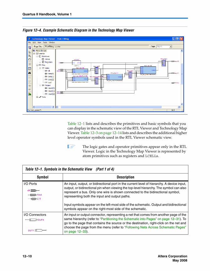
Figure 12–4 shows a portion of the corresponding Technology Map Viewer schematic with a compiled design that targets a Stratix® device. In this schematic, you can see the LCELL (logic cell) device-specific primitives that represent the counter function, labeled with their post-synthesis node names. The REGOUT port represents the output of the register in the LCELL; the COMBOUT port represents the output of the combinational logic in the LUT of the LCELL. The hexadecimal number in parentheses below each LCELL primitive represents the LUT mask, which is a hexadecimal representation of the logic function of the LCELL.



Figure 12–4. Example Schematic Diagram in the Technology Map Viewer

Table 12–1 lists and describes the primitives and basic symbols that you can display in the schematic view of the RTL Viewer and Technology Map Viewer. Table 12–3 on page 12–14 lists and describes the additional higher level operator symbols used in the RTL Viewer schematic view.

1 The logic gates and operator primitives appear only in the RTL Viewer. Logic in the Technology Map Viewer is represented by atom primitives such as registers and LCELLs.

Table 12–1. Symbols in the Schematic View (Part 1 of 4)

Symbol Description

I/O Ports An input, output, or bidirectional port in the current level of hierarchy. A device input, output, or bidirectional pin when viewing the top-level hierarchy. The symbol can also represent a bus. Only one wire is shown connected to the bidirectional symbol, representing both the input and output paths.

Input symbols appear on the left-most side of the schematic. Output and bidirectional symbols appear on the right-most side of the schematic.

I/O Connectors An input or output connector, representing a net that comes from another page of the same hierarchy (refer to “Partitioning the Schematic into Pages” on page 12–31). To go to the page that contains the source or the destination, right-click on the net and choose the page from the menu (refer to “Following Nets Across Schematic Pages” on page 12–33).



Hierarchy Port Connector A connector representing a port relationship between two different hierarchies. A connector indicates that a path passes through a port connector in a different level of hierarchy.

OR, AND, XOR Gates An OR, AND, or XOR gate primitive (the number of ports can vary). A small circle (bubble symbol) on an input or output port indicates the port is inverted.

MUX A multiplexer (MUX) primitive with a selector port that selects between port 0 and port 1. A MUX with more than two inputs is displayed as an operator (refer to “Operator Symbols in the RTL Viewer Schematic View” on page 12–14).

BUFFER A buffer primitive. The figure shows the tri-state buffer, with an inverted output enable port. Other buffers without an enable port include LCELL, SOFT, CARRY, and GLOBAL. The NOT gate and EXP expander buffers use this symbol without an enable port and with an inverted output port.

CARRY_SUM A CARRY_SUM buffer primitive with the following ports:● SI – SUM IN● SO – SUM OUT● CI – CARRY IN● CO – CARRY OUT

LATCH A latch primitive with the following ports: ● D – data input● ENA – enable input● Q – data output● PRE – preset● CLR – clear

DFFE/DFFEA/DFFAES A DFFE (data flipflop with enable) primitive, with the same ports as a latch and a clock trigger. The other flipflop primitives are similar: ● DFFEA (data flipflop with enable and asynchronous load) primitive with additional

ALOAD asynchronous load and ADATA data signals● DFFEAS (data flipflop with enable and both synchronous and asynchronous

load), which has ASDATA as the secondary data port


Symbol Description



Atom Primitive Primitives are low-level nodes that cannot be expanded to any lower hierarchy. The symbol displays the port names, the primitive type, and its name. The blue shading indicates an atom primitive in the Technology Map Viewer that allows you to view the internal details of the primitive. Refer to “Viewing Contents of Atom Primitives” on page 12–22 for details.

Other Primitive Any primitive that does not fall into the categories above. Primitives are low-level nodes that cannot be expanded to any lower hierarchy. The symbol displays the port names, the primitive or operator type, and its name.

The figure shows an LCELL WYSIWYG primitive, with DATAA to DATAD and COMBOUT port connections. This type of LCELL primitive is found in the Technology Map Viewer for technology-specific atom primitives when the contents of the atom primitive cannot be viewed. The RTL Viewer contains similar primitives if the source design is a VQM or EDIF netlist.

Instance An instance in the design that does not correspond to a primitive or operator (generally a user-defined hierarchy block), indicated by the double outline and green shading. The symbol displays the instance name.

To open the schematic for the lower level hierarchy, right-click and choose the appropriate command (refer to “Traversing and Viewing the Design Hierarchy” on page 12–21).

Encrypted Instance A user-defined encrypted instance in the design, indicated by the double outline and gray shading. The symbol displays the instance name. You cannot open the schematic for the lower level hierarchy, because the source design is encrypted.

State Machine Instance A finite state machine instance in the design, indicated by the double outline and yellow shading. Double-clicking this instance opens the State Machine Viewer. Refer to “State Machine Viewer” on page 12–18 for more details.

RAM A synchronous memory instance with registered inputs and optionally registered outputs, indicated by purple shading. The symbol shows the device family and the type of TriMatrix memory block. This figure shows a true dual-port memory block in a Stratix M-RAM block.


Symbol Description



Table 12–2 lists and describes the symbol used only in the State Machine Viewer.

Logic Cloud A logic cloud is a group of combinational logic, indicated by a cloud symbol. Refer to “Grouping Combinational Logic into Logic Clouds” on page 12–27 for more details.

Constant A constant signal value that is highlighted in gray and displayed in hexadecimal format by default throughout the schematic. To change the format, refer to “Changing the Constant Signal Value Formatting” on page 12–29.


Symbol Description

Table 12–2. Symbol Available Only in the State Machine Viewer

Symbol Description

State Node The node representing a state in a finite state machine. State transitions are indicated with arcs between state nodes. The double circle border indicates the state connects to logic outside the state machine, while a single circle border indicates the state node does not feed outside logic.



Table 12–3 lists and describes the additional higher level operator symbols used in the RTL Viewer schematic view.

Table 12–3. Operator Symbols in the RTL Viewer Schematic View (Part 1 of 2)

Symbol Description

An adder operator:OUT = A + B

A multiplier operator:OUT = A × B

A divider operator:OUT = A / B

Equals

A left shift operator:OUT = (A << COUNT)

A right shift operator:OUT = (A >> COUNT)



Selecting an Item in the Schematic View

To select an item in the schematic view, ensure that the Selection Tool is enabled in the viewer toolbar (this tool is enabled by default). Click on an item in the schematic view to highlight it in red.

Select multiple items by pressing the Shift or Ctrl key while selecting with your mouse. You can also select all nodes in a region by selecting a rectangular box area with your mouse cursor when the Selection Tool is enabled. To select nodes in a box, move your mouse to one corner of the area you want to select, click the mouse button, and drag the mouse to the opposite corner of the box, then release the mouse button. By default,

A modulo operator:OUT = (A % B)

A less than comparator:OUT = (A < B : A > B)

A multiplexer:OUT = DATA [SEL]The data range size is 2sel range size

A selector:A multiplexer with one-hot select input and more than two input signals

A binary number decoder:OUT = (binary_number (IN) == x)for x = 0 to x = 2(n+1) - 1

Table 12–3. Operator Symbols in the RTL Viewer Schematic View (Part 2 of 2)

Symbol Description



creating a box like this highlights and selects all nodes in the selected area (instances, primitives, and pins), but not the nets. The Viewer Options dialog box provides an option to select nets. To include nets, right-click in the schematic and click Viewer Options. In the Net Selection section, turn on the Select entire net when segment is selected option.

Items selected in the schematic view are automatically selected in the hierarchy list (refer to the “Hierarchy List” on page 12–17). The list expands automatically if required to show the selected entry. However, the list does not collapse automatically when entries are not being used or are deselected.

When you select a hierarchy box, node, or port in the schematic view, the item is highlighted in red but none of the connecting nets are highlighted. When you select a net (wire or bus) in the schematic view, all connected nets are highlighted in red. The selected nets are highlighted across all hierarchy levels and pages. Net selection can be useful when navigating a netlist because you see the net highlighted when you traverse between hierarchy levels or pages.

In some cases, when you select a net that connects to nets in other levels of the hierarchy, these connected nets also are highlighted in the current hierarchy. If you prefer that these nets not be highlighted, use the Viewer Options dialog box option to highlight a net only if the net is in the current hierarchy. Right-click in the schematic and click Viewer Options. In the Net Selection section, turn on the Limit selections to current hierarchy option.

Moving and Panning in the Schematic View

When the schematic view page is larger than the portion currently displayed, you can use the scroll bars at the bottom and right side of the schematic view to see other areas of the page.

You can also use the Hand Tool to “grab” the schematic page and drag it in any direction. Enable the Hand Tool with the toolbar button. Click and drag to move around the schematic view without using the scroll bars.

In addition to the scroll bars and Hand Tool, you can use the middle-mouse/wheel button to move and pan in the schematic view. Click the middle-mouse/wheel button once to enable the feature. Move the mouse or scroll the wheel to move around the schematic view. Click the middle-mouse/wheel button again to turn the feature off.



Hierarchy List

The hierarchy list is displayed on the left side of the viewer window. The hierarchy list displays the entire netlist in a tree format based on the hierarchical levels of the design. Within each level, similar elements are grouped into sub-categories. Using the hierarchy list, traverse through the design hierarchy to view the logic schematic for each level. You can also select an element in the hierarchy list to be highlighted in the schematic view.

1 Nodes inside atom primitives are not listed in the hierarchy list.

For each module in the design hierarchy, the hierarchy list displays the applicable elements listed in Table 12–4. Click the + icon to expand an element.

Table 12–4. Hierarchy List Elements

Elements Description

Instances Modules or instances in the design that can be expanded to lower hierarchy levels.

State Machines State machine instances in the design that can be viewed in the State Machine Viewer.

Primitives Low-level nodes that cannot be expanded to any lower hierarchy level. These include:● Registers and gates that you can view in the RTL Viewer when using Quartus II integrated

synthesis● Logic cell atoms in the Technology Map Viewer or in the RTL Viewer when using a VQM

or EDIF from third-party synthesis softwareIn the Technology Map Viewer, you can view the internal implementation of certain atom primitives, but you can not traverse into a lower level of hierarchy.

Pins The I/O ports in the current level of hierarchy.● Pins are device I/O pins when viewing the top hierarchy level, and are I/O ports of the

design when viewing the lower levels.● When a pin represents a bus or an array of pins, expand the pin entry in the list view to see

individual pin names.

Nets Nets or wires connecting the nodes. When a net represents a bus or array of nets, expand the net entry in the tree to see individual net names.

Logic Clouds A group of related combinational logics of a particular source. You can automatically or manually group combinational logics or ungroup logic clouds in your design.



Selecting an Item in the Hierarchy List

When you click any item in the hierarchy list, the viewer performs the following actions:

■ Searches for the item in the currently viewed pages and displays the page containing the selected item in the schematic view if it is not currently displayed. (If you are currently viewing a filtered netlist, for example, the relevant page within the filtered netlist is displayed.)

■ If the selected item is not found in the currently viewed pages, the entire design netlist is searched and the item is displayed in a default view.

■ Highlights the selected item in red in the schematic view.

When you double-click an instance in the hierarchy list, the viewer displays the underlying implementation of the instance.

You can select multiple items by pressing the Shift or Ctrl key while selecting with your mouse. When you right-click an item in the hierarchy list, you can navigate in the schematic view using the Filter and Locate commands. Refer to “Filtering in the Schematic View” on page 12–36 and “Probing to Source Design File and Other Quartus II Windows” on page 12–44 for more information.

State Machine Viewer

The State Machine Viewer displays a graphical representation of the state machines in your design. You can open the State Machine Viewer in any of the following ways:

■ On the Tools menu, point to Netlist Viewers and click State Machine Viewer

■ Double-click on a state machine instance in the RTL Viewer■ Right-click on a state machine instance in the RTL Viewer and click

Hierarchy Down■ Select a state machine instance in the RTL Viewer, and on the Project

menu, point to Hierarchy and click Down

Figure 12–5 shows an example of the State Machine Viewer for a simple state machine. The State Machine toolbar on the left side of the viewer provides tools you can use in the state diagram view.



Figure 12–5. State Machine in the State Machine Viewer

State Diagram View

The state diagram view is shown at the top of the State Machine Viewer window. It contains a diagram of the states and state transitions.

The nodes that represent each state are arranged horizontally in the state diagram view with the initial state (the state node that receives the reset signal) in the left-most position. Nodes that connect to logic outside of the state machine instance are represented by a double circle. The state transition is represented by an arc with an arrow pointing in the direction of the transition.

When you select a node in the state diagram view, if you turn on the Highlight Fan-in or Highlight Fan-out command from the View menu or the State Machine Viewer toolbar, the respective fan-in or fan-out transitions from the node are highlighted in red.



1 An encrypted block with a state machine displays encoding information in the state encoding table, but does not display a state transition diagram or table.

State Transition Table

The state transition table on the Transitions tab at the bottom of the State Machine Viewer window displays the condition equation for each state transition. Each transition (each arc in the state diagram view) is represented by a row in the table. The table has the following three columns:

■ Source State—the name of the source state for the transition■ Destination State—the name of the destination state for the

transition■ Condition—the condition equation that causes the transition from

source state to destination state

To see all of the transitions to and from each state name, click the appropriate column heading to sort on that column.

The text in each column is left-aligned by default; to change the alignment and more easily see the relevant part of the text, right-click in the column and click Align Right. To change back to left alignment, click Align Left.

Click in any cell in the table to select it. To select all cells, right-click in the cell and click Select All; or, on the Edit menu, click Select All. To copy selected cells to the clipboard, right-click the cells and click Copy Table; or, on the Edit menu, point to Copy and click Copy Table. You can paste the table into any text editor as tab-separated columns.

State Encoding Table

The state encoding table on the Encoding tab at the bottom of the State Machine Viewer window displays encoding information for each state transition.

To view state encoding information in the State Machine Viewer, you must have synthesized your design using Start Analysis & Synthesis. If you have only elaborated your design using Start Analysis & Elaboration, the encoding information is not displayed.

Selecting an Item in the State Machine Viewer

You can select and highlight each state node and transition in the State Machine Viewer. To select a state transition, click the arc that represents the transition.


Navigating the Schematic View

When you select a state node, transition arc, or both in the state diagram view, the matching state node and equation conditions in the state transition table are highlighted. Conversely, when you select a state node, equation condition, or both in the state transition table, the corresponding state node and transition arc are highlighted in the state diagram view.

Switching Between State Machines

A design may contain multiple state machines. To choose which state machine to view, use the State Machine selection box located at the top of the State Machine Viewer. Click in the drop-down box and select the desired state machine.


The previous sections provided an overview of the user interface for each netlist viewer, and how to select an item in each viewer. This section describes methods to navigate through the pages and hierarchy levels in the schematic view of the RTL Viewer and Technology Map Viewer.

Traversing and Viewing the Design Hierarchy

You can open different hierarchy levels in the schematic view using the hierarchy list (refer to “Hierarchy List” on page 12–17), or the Hierarchy Up and Hierarchy Down commands in the schematic view.

Use the Hierarchy Down command to go down into, or expand an instance’s hierarchy, and open a lower level schematic showing the internal logic of the instance. Use the Hierarchy Up command to go up in hierarchy, or collapse a lower level hierarchy, and open the parent higher level hierarchy. When the Selection Tool is selected, the appropriate option is available when your mouse pointer is located over an area of the schematic view that has a corresponding lower or higher level hierarchy.

The mouse pointer changes as it moves over different areas of the schematic to indicate whether you can move up, down, or both up and down in the hierarchy (Figure 12–6). To open the next hierarchy level, right-click in that area of the schematic and click Hierarchy Down or Hierarchy Up, as appropriate, or double-click in that area of the schematic.

Figure 12–6. Mouse Pointers Indicate How to Traverse Hierarchy



Flattening the Design Hierarchy

You can flatten the design hierarchy to view the design without hierarchical boundaries. To flatten the hierarchy from the current level and all the lower level hierarchies of the current design hierarchy, right-click in the schematic and click Flatten Netlist. To flatten the entire design, choose Flatten Netlist from the top-level schematic of the design.

Viewing the Contents of a Design Hierarchy within the Current Schematic

You can use the Display Content and Hide Content commands to show or hide a lower hierarchy level for a specific instance within the schematic for the current hierarchy level.

To display the lower hierarchy netlist of an instance on the same schematic as the remaining logic in the currently viewed netlist, right-click the selected instance and click Display Content.

To hide all of the lower hierarchy logic of a hierarchy box into a closed instance, right-click the selected instance and click Hide Content.

Viewing Contents of Atom Primitives

In the Technology Map Viewer, you can view the contents of certain device atom primitives to see their underlying implementation details. For logic cell (LCELL) atoms in the Stratix and Cyclone® series of devices, in Arria GX devices, and in MAX® II devices, you can view LUTs, registers, and logic gates. For I/O atoms in the Stratix and Cyclone series of devices, in Arria GX devices, and HardCopy® II devices, you can view registers and logic gates.

In addition, you can view the implementation of RAM and DSP blocks in certain devices in the RTL Viewer or Technology Map Viewer. You can view the implementation of RAM blocks in the Stratix and Cyclone series of devices, and in Arria GX devices. You can view the implementation of DSP blocks only in the Stratix series of devices and Arria GX devices.

If you can view the contents of an atom instance, it is blue in the schematic view (Figure 12–7).



Figure 12–7. Instance That Can Be Expanded to View Internal Contents

To view the contents of one or more atom primitive instances, select the desired atom instances. Right-click a selected instance and click Display Content. You can also double-click on the desired atom instance to view the contents. Figure 12–8 shows an expanded version of the instance in Figure 12–7.

Figure 12–8. Internal Contents of the Atom Instance in Figure 12–7.

To hide the contents (and revert to the compact format), select and right-click the atom instance(s), and click Hide Content.

1 In the schematic view, the internal details within an atom instance can not be selected as individual nodes. Any mouse action on any of the internal details is treated as a mouse action on the atom instance.



Viewing the Properties of Instances and Primitives

You can view the properties of an instance or primitive using the Properties dialog box. To view the properties of an instance or a primitive in the RTL Viewer or Technology Map Viewer, right-click the node and click Properties.

The Properties dialog box contains the following information about the selected node:

■ The parameter values of an instance.■ The active level of the port (for example, active high or active low).

An active low port is denoted with an exclamation mark “!”.■ The port’s constant value (for example, VCC or GND). Table 12–5

describes the possible value of a port.

In the look-up-table (LUT) of a logic cell (LCELL), the Properties dialog box contains the following additional information:

■ The schematic of the LCELL.■ The Truth Table representation of the LCELL.■ The Karnaugh map representation of the LCELL.

Viewing LUT Representations in the Technology Map Viewer

You can view different representations of an LUT by right-clicking on the selected LUT and selecting Properties. This feature is supported for the Stratix and Cyclone series of devices, Arria GX devices, and MAX II devices only. There are three tabs in the Properties dialog box, which you can choose from to view the LUT representations:

■ The Schematic tab (see Figure 12–9) shows you the equivalent gate representations of the LUT.

■ The Truth Table tab (see Figure 12–10) shows the truth table representations.

Table 12–5. Possible Port Values

Value Description

VCC The port is not connected and has VCC value (tied to VCC)

GND The port is not connected and has GND value (tied to GND)

-- The port is connected and has value (other than VCC or GND)

Unconnected The port is not connected and has no value (hanging)



■ The Karnaugh Map tab (see Figure 12–11) shows the Karnaugh map representations of the LUT. The Karnaugh map supports up to 6 input LUTs.

For details about the Ports tab, see “Viewing the Properties of Instances and Primitives”.

Figure 12–9. Schematic Tab



Figure 12–10. Truth Table Tab

Figure 12–11. Karnaugh Map Tab



Grouping Combinational Logic into Logic Clouds

This following sections describes how to group combinational logic into logic clouds.

1 For the definition of a logic cloud, refer to Table 12–1 on page 12–10.

Logic Clouds in the RTL Viewer

You can automatically group all combinational logic nodes in your design into logic clouds. On the Tools menu, click Options on the Tools menu, and in the Category list, expand Netlist Viewers and select RTL Viewer. On the RTL Viewer page, turn on Group combinational logic into logic cloud. You can also turn on this option by right-clicking in the schematic and clicking Viewer Options. In the RTL/Technology Map Viewer Options dialog box, click the Customize View tab. In the Customize Groups section, turn on Group combinational logic into logic cloud. Figure 12–12 and Figure 12–13 show the schematic before and after the combinational logic grouping operation in the RTL Viewer.

Logic Clouds in the Technology Map Viewer

In the Technology Map Viewer, the Group combinational logic into logic clouds option is supported for the Stratix II, Cyclone II, and Hardcopy families of devices only. To set this option, right-click in the schematic and click Viewer Options. In the RTL/Technology Map Viewer Options dialog box, click on the Customize View tab. Turn on the Group combinational logic into logic cloud option.



Figure 12–12. Schematic Before Combinational Logic Grouping

Figure 12–13. Schematic After Combinational Logic Grouping



Manually Group and Ungroup Logic Clouds

To group logic nodes into a logic cloud manually, right-click the selected node or input port and select Group source logic into logic cloud. To ungroup a logic cloud manually, right-click on the selected logic cloud and select Ungroup source logic from logic cloud. You can also ungroup a logic cloud manually by double-clicking on the selected logic cloud. These options are not available if the nodes cannot be grouped.

Changing the Constant Signal Value Formatting

The constant signal value is highlighted in gray in the schematic view. By default, the value is displayed in hexadecimal format, but you can also choose binary or decimal format. To change the value formatting, on the Tools menu, click Options. In the Category list, select Netlist Viewers, and select the desired format from the Constant Signal Format list.

Changing the format affects all constant signal value throughout the schematic. Refer to Table 12–3 on page 12–14 to see what constant signal values look like in the schematic.

Zooming and Magnification

You can control the magnification of your schematic with the View menu, the Zoom Tool in the toolbar, or the Ctrl key and mouse wheel button, as described in this section.

The Fit in Window, Fit Selection in Window, Zoom In, Zoom Out, and Zoom commands are available from the View menu, by right-clicking in the schematic view and selecting Zoom, or from the Zoom toolbar. To enable the zoom toolbar, on the Tools menu, click Customize. Click the Toolbars tab and click Zoom to enable the toolbar.

By default, the viewer displays most pages sized to fit in the window. If the schematic page is very large, the schematic is displayed at the minimum zoom level, and the view is centered on the first node. Select Zoom In to view the image at a larger size, and select Zoom Out to view the image (when the entire image is not displayed) at a smaller size. The Zoom command allows you to specify a magnification percentage (100% is considered the normal size for the schematic symbols). To change the minimum and maximum zoom level, on the Tools menu, click Options. In the Options dialog box, in the Category list, select Netlist Viewers and set the desired minimum and maximum zoom level.

The Fit Selection in Window command zooms in on the selected nodes in a schematic to fit within the window. Use the Selection Tool to select one or more nodes (instances, primitives, pins, and nets), then select Fit



Selection in Window to enlarge the area covered by the selection. This feature is helpful when you want to see a particular element in a large schematic. After you select a node, you can easily zoom in to view the particular node.

You can also use the Zoom Tool on the viewer toolbar to control magnification in the schematic view. When you select the Zoom Tool in the toolbar, clicking on the schematic zooms in and centers the view on the location you clicked. Right-click on the schematic to zoom out and center the view on the location you clicked. When you select the Zoom Tool, you can also zoom in to a certain portion of the schematic by selecting a rectangular box area with your mouse cursor. The schematic is enlarged to show the selected area.

Alternatively, using the Zoom Tool, you can specify the magnification percentage by right-clicking on the desired area and dragging the mouse toward your right to zoom in or toward your left to zoom out. You will see a green line with the zoom percentage on top. The zoom percentage is proportional to the length of the green line (Figure 12–14). Release the mouse button at the desired zoom percentage.

Figure 12–14. Dragging the Mouse Pointer to Change Zoom Percentage



By default, the viewers maintain the zoom level when filtering on the schematic (refer to “Filtering in the Schematic View” on page 12–36). To change the behavior so that the zoom level is always reset to “Fit in Window,” on the Tools menu, click Options. In the Category list, select Netlist Viewers, and turn off Maintain zoom level.

Schematic Debugging and Tracing Using the Bird's Eye View

Viewing the entire schematic can be useful when debugging and tracing through a large netlist. The Quartus II software allows you to view the entire schematic in a single window. The bird’s eye view is displayed in a separate window that is linked directly to the netlist viewers. This feature is available in the RTL, Technology Map, and Technology Map (Post-Mapping) viewers.

The bird’s eye view shows the current area of interest. Select the desired area by clicking and dragging the indicator or using the right-mouse button to form a rectangular box around the desired area. You can also click and drag the rectangular box to move around the schematic. To open the bird’s eye view, on the View menu, click Bird’s Eye View, or click on the Bird’s Eye View icon in the Viewer toolbar (Figure 12–15).

Figure 12–15. Bird’s Eye View and Full Screen Icon

Full Screen View

To set the viewer window to fill the whole screen, on the View menu, click Full Screen, or click the Full Screen icon in the viewer toolbar (Figure 12–15), or press Ctrl+Alt+Space. The keyboard shortcut toggles between the full screen and standard screen views.

Partitioning the Schematic into Pages

For large design hierarchies, the RTL Viewer and Technology Map Viewer partition your netlist into multiple pages in the schematic view. To control how much of the design is visible on each page, on the Tools menu, click Options. In the Category list, select Netlist Viewers and set the desired options under Display Settings.

Bird’s Eye View icon

Full Screen Icon



The Nodes per page option specifies the number of nodes per partitioned page. The default value is 50 nodes; the range is 1 to 1,000 nodes. The Ports per page option specifies the number of ports (or pins) per partitioned page. The default value is 1,000 ports (or pins); the range is 1 to 2,000 ports (or pins). The viewers partition your design into a new page if either the node number or the port number exceeds the limit you have specified. You may occasionally see the number of ports exceed the limit, depending on the configuration of nodes on the page.

If the Display boundary around hierarchy levels option is turned on, and the total number of nodes or ports within the hierarchy exceeds the value of Nodes per page or Ports per page, the boundary is displayed as a hierarchy port connector (refer to Table 12–1 on page 12–10). For more information about the Display boundary around hierarchy levels option, refer to “Filtering Across Hierarchies” on page 12–40.

When a hierarchy level is partitioned into multiple pages, the title bar for the schematic window indicates which page is displayed and how many total pages exist for this level of hierarchy (shown in the format: Page <current page number> of <total number of pages>), as shown in Figure 12–16.

Figure 12–16. RTL Viewer Title Bars Indicating Page Number Information

When you change the number of nodes or ports per page, the change applies only to new pages that are shown or opened in the viewer. To refresh the current page so that it displays the changed number of nodes or ports, click the Refresh button in the toolbar.

Moving between Schematic Pages

To move to another schematic page, on the View menu, click Previous Page or Next Page, or click the Previous Page icon or the Next Page icon in the viewer toolbar.



To go to a particular page of the schematic, on the Edit menu, click Go To, or right-click in the schematic view and click Go To. In the Page list, select the desired page number. You can also go to a particular page by selecting the desired page number from the pull-down list on the top right of the viewer window.

Moving Back and Forward Through Schematic Pages

To return to the previous view after changing the page view, click Back on the View menu, or click the Back icon on the viewer toolbar. To go to the next view, click Forward on the View menu, or click the Forward icon on the viewer toolbar.

1 You can go Forward only if you have not made any changes to the view since going Back. Use Back and Forward to switch between page views. These commands do not undo an action such as selecting a node.

Following Nets Across Schematic Pages

Input and output connectors indicate nodes that connect across pages of the same hierarchy. Right-click on a connector to display a menu of commands that trace the net through the pages of the hierarchy.

1 After you right-click to follow a connector port, the viewer opens a new page, which centers the view on the particular source or destination net using the same zoom factor used by the previous page. To trace a specific net to the new page of the hierarchy, Altera recommends that you first select the desired net, which highlights it in red, before you right-click to traverse pages.

Input ConnectorsFigure 12–17 shows an example of the menu that appears when you right-click an input connector. The From command opens the page containing the source of the signal. The Related commands, if applicable, open the specified page containing another connection fed by the same source.



Figure 12–17. Input Connector Right Button Pop-Up Menu

Output ConnectorsFigure 12–18 shows an example of the menu that appears when you right-click an output connector. The To command opens the specified page that contains a destination of the signal.

Figure 12–18. Output Connector Right Button Pop-Up Menu


Customizing the Schematic Display in the RTL Viewer

Go to Net Driver

To locate the source of a particular net in the schematic view, select the net to highlight it, right-click the selected net, point to Go to Net Driver, and click Current page, Current hierarchy, or Across hierarchies. Refer to Table 12–6 for details.

The schematic view opens the correct page of the schematic if needed, and adjusts the centering of the page so that you can see the net source. The schematic shows the default page for the net driver. The view is an unfiltered view, so no filtering results are kept.

Customizing the Schematic Display in the RTL Viewer

You can customize the schematic display for better viewing and to speed up your debugging process. The options that control the schematic display are available in the Customize View tab of the RTL/Technology Map Viewer Options dialog box. To open the dialog box, right-click in the schematic and click Viewer Options. You can turn on the options to remove fan-out free nodes, simplify logic, group or ungroup related nodes, and group combinational logic into a logic cloud.

You can also customize the schematic view in the RTL Viewer by clicking Options on the Tools menu. In the Category list, expand Netlist Viewers and select RTL Viewer. Set the desired customization for your schematic display.

1 When the settings are changed, the list of previously viewed pages is cleared. The settings are revision-specific, so different revisions can have different settings.

To remove fan-out free registers from your schematic display, turn on Remove registers without fan-out. By default, this option is turned on.

To remove all single-input nodes and merge a chain of equivalent combinational gates that have direct connections (without inversion in between) into a single multiple-input gate, turn on Show simplified logic. By default, this option is turned on.

Table 12–6. Go to Net Driver Commands

Command Action

Current page Locates the source or driver on the current page of the schematic only.

Current hierarchy Locates the source within the current level of hierarchy, even if the source is located on another page of the netlist schematic.

Across hierarchies Locates the source across hierarchies until the software reaches the source at the top hierarchy level.



To group all related nodes into a single node, turn on Group all related nodes. This option is turned on by default. You can manually group or ungroup any nodes by right-clicking the selected nodes in the schematic and selecting Group Related Nodes to group or Ungroup Selected Nodes to ungroup.

Filtering in the Schematic View

Filtering allows you to filter out nodes and nets in your netlist to view only the logic that interests you.

Filter your netlist by selecting hierarchy boxes, nodes, ports of a node, nets, or states in a state machine that are part of the path you want to see. The following filter commands are available:

■ Sources—Displays the sources of the selection■ Destinations—Displays the destinations of the selection■ Sources & Destinations—Displays both the sources and

destinations of the selection■ Selected Nodes and Nets—Displays only the selected nodes and

nets with the connections between them■ Between Selected Nodes—Displays nodes and connections in the

path between the selected nodes ■ Bus Index—Displays the sources or destinations for one or more

indices of an output or input bus port

Select a hierarchy box, node, port, net, or state node, right-click in the window, point to Filter and click the appropriate filter command. The viewer generates a new page showing the netlist that remains after filtering.

When filtering in a state diagram in the State Machine Viewer, sources and destinations refer to the previous and next transition states or paths between transition states in the state diagram. The transition table and encoding table also reflect the filtering.

You can go back to the netlist page before it was filtered using the Back command, described in “Moving Back and Forward Through Schematic Pages” on page 12–33.

1 When viewing a filtered netlist, clicking an item in the hierarchy list causes the schematic view to display an unfiltered view of the appropriate hierarchy level. You cannot use the hierarchy list to select items or navigate in a filtered netlist.



Filter Sources Command

To filter out all but the source of the selected item, right click the item, point to Filter and click Sources. The selected object type determines what is displayed, as outlined in Table 12–7 and shown in Figure 12–19 on page 12–38.

Filter Destinations Command

To filter out all but the destinations of the selected node or port as outlined in Table 12–8 and shown in Figure 12–19 on page 12–38, right-click the node or port, point to Filter and click Destinations.

Table 12–7. Selected Objects Determine Filter Sources Display

Selected Object Result Shown in Filtered Page

Node or hierarchy box Shows all the sources of the node’s input ports. For an example, refer to Figure 12–19 on page 12–38.

Net Shows the sources that feed the net.

Input port of a node Shows only the input source nodes that feed this port.

Output port of a node Shows only the selected node.

State node in a state machine Shows the states that feed the selected state (previous transition states).

Table 12–8. Selected Objects Determine Filter Destinations Display

Selected Object Result Shown in Filtered Page

Node or hierarchy box Shows all the destinations of the node’s output ports. For an example, refer to Figure 12–19 on page 12–38.

Net Shows the destinations fed by the net.

Input port of a node Shows only the selected node.

Output port of a node Shows only the fan-out destination nodes fed by this port.

State node in a state machine Shows the states that are fed by the selected states (next transition states).



Filter Sources and Destinations Command

The Sources & Destinations command is a combination of the Sources and Destinations filtering commands, in which the filtered page shows both the sources and the destinations of the selected item. To select this option, right-click on the desired object, point to Filter and click Sources & Destinations. Refer to the example in Figure 12–19.

Figure 12–19. Sources, Destinations, and Sources and Destinations Filtering for inst4

Filter Between Selected Nodes Command

To show the nodes in the path between two or more selected nodes or hierarchy boxes, right-click, point to Filter and click Between Selected Nodes. For this option, selecting a port of a node is the same as selecting the node. For an example, refer to Figure 12–20.

Figure 12–20. Between Selected Nodes Filtering Between inst2 and inst3

inst2inst4pin_name3

pin_name4

pin_name3

pin_name4inst2OUT1

inst4OUT1inst3OUT1

pin_name5 pin_name6instOUT1

Sources & Destinations

Sources

Destinations

inst3

instpin_name

pin_name2

pin_name5

pin_name

pin_name2

Selected Node

inst2inst4pin_name3

pin_name4

pin_name3

pin_name4inst2OUT1

inst4OUT1inst3OUT1

pin_name5 pin_name6instOUT1

inst3

instpin_name

pin_name2

pin_name5

pin_name

pin_name2

Between Selected Nodes

Selected Nodes



Filter Selected Nodes and Nets Command

To create a filtered page that shows only the selected nodes, nets, or both, and, if applicable, the connections between the selected nodes, nets, or both, right-click, point to Filter, and click Selected Nodes & Nets. Figure 12–21 shows a schematic with several nodes selected.

Figure 12–21. Using Selected Nodes and Nets to Select Nodes

Figure 12–22 shows the schematic after filtering has been performed. If you select a net, the filtered page shows the immediate sources and destinations of the selected net.

Figure 12–22. Selected Nodes and Nets Filtering on Figure 12–21 Schematic

Filter Bus Index Command

To show the path related to a specific index of a bus input or output port in the RTL Viewer, right-click the port, point to Filter, and click Bus Index. The Select Bus Index dialog box allows you to select the indices of interest.

Selected Nodes



Filter Command Processing

The options to control filtering are available in the Tracing section of the RTL/Technology Map Viewer Options dialog box. Right-click in the schematic and click Viewer Options to open the dialog box.

For all the filtering commands, the viewer stops tracing through the netlist to obtain the filtered netlist when it reaches one of the following objects:

■ A pin■ A specified number of filtering levels, counting from the selected

node or port; the default value is 3

1 Specify the Number of filtering levels in the Tracing section of the RTL/Technology Map Viewer Options dialog box. The default value is 3 to ensure optimal processing time when performing filtering, but you can specify a value from 1 to 100.

■ A register (optional; turned on by default)

1 Turn the Stop filtering at register option on or off in the Tracing section of the RTL/Technology Map Viewer Options dialog box. Right-click in the schematic and click Viewer Options to open the dialog box.

By default, the filtered schematic shows all possible connections between the nodes shown in the schematic. To remove the connections that are not directly part of the path that was traced to generate a filtered netlist, turn off the Shows all connections between nodes option in the Tracing section of the RTL/Technology Map Viewer Options dialog box.

Filtering Across Hierarchies

The filtering commands display nodes in all hierarchies by default. When the filtered path passes through levels of hierarchy on the same schematic page, green hierarchy boxes group the logic and show the hierarchy boundaries. A green rectangular symbol appears on the border that represents the port relationship between two different hierarchies (Figure 12–23 and Figure 12–24).

The RTL/Technology Map Viewer Options dialog box provides an option to control filtering if you prefer to filter only within the current hierarchy. Right-click in the schematic and click Viewer Options. In the Tracing section, turn off the Filter across hierarchy option.



To disable the box hierarchy display, on the Tools menu, click Options. In the Category list, select Netlist Viewers and turn off Display boundary around hierarchy levels.

1 Netlists of the same hierarchy that are displayed over more than one page are not grouped with a box. Filtering and expanding on a blue atom primitive does not trace the underlying netlist even when Filter across hierarchy is enabled.

Figures 12–23 and 12–24 show examples of filtering across hierarchical boundaries. Figure 12–23 shows an example after the Sources filter has been applied to an input port of the taps instance, where the input port of the lower level hierarchical block connects directly to an input pin of the design. The name of the instance is indicated within the green border and appears as a tooltip when you move your mouse pointer over the instance.

Figure 12–23. Filtering Across Hierarchical Boundaries, Small Example



Figure 12–24 shows a larger example after the Sources filter has been applied to an input port of an instance, in which the source comes from input pins that are fed through another level of hierarchy.

Figure 12–24. Filtering Across Hierarchical Boundaries, Large Example

Expanding a Filtered Netlist

After a netlist is filtered, some ports may have no connections displayed because their connections are not part of the main path through the netlist. Two expansion features, immediate expansion and the Expand command, allow you to add the fan-in or fan-out signals of these ports to the schematic display of a filtered netlist.

You can immediately expand any port whose connections are not displayed. When you double-click that port in the filtered schematic, one level of logic is expanded.

To expand more than one level of logic, right-click the port and click the Expand command. This command expands logic from the selected port by the amount specified in Viewer Options. To set these options, right-click in the schematic view and click Viewer Options. In the Expansion section, set the Number of expansion levels option to specify the number of levels to expand (the default value is 3 and the range is 1 to 100 levels).

Hierarchical Boundary



You can also set the Stop expanding at register option (which is turned on by default) to specify whether netlist expansion should stop when a register is reached.

You can select multiple nodes to expand when using the Expand command. If you select ports that are located on multiple schematic pages, only the ports on the currently viewed page appear in the expanded schematic.

In the State Machine Viewer, the Expand command has the following three options:

■ Sources—Displays the states that feed the selected states (previous transition states)

■ Destinations—Displays the states that are fed by the selected states (next transition states)

■ Sources & Destinations—Displays both the previous and next transition states

The state transition table and state encoding table also reflect the changes to the filtering.

The expansion feature works across hierarchical boundaries if the filtered page containing the port to be expanded was generated with the Filter across hierarchy option turned on (refer to “Filtering in the Schematic View” on page 12–36 for details about this option). When viewing timing paths in the Technology Map Viewer, the Expand command always works across hierarchical boundaries because filtering across hierarchy is always turned on for these schematics (refer to “Viewing a Timing Path” on page 12–47 for details on these schematics).

Reducing a Filtered Netlist

In some cases, removing logic from a filtered schematic or state diagram makes the schematic view easier to read or minimizes distracting logic that you do not need to view in the schematic.

To reduce elements in the filtered schematic or state diagram view, right-click the node or nodes you want to remove and click Reduce.



Probing to Source Design File and Other Quartus II Windows

The RTL, Technology Map, and State Machine Viewers let you cross-probe from the viewer to the source design file and to various other windows within the Quartus II software. You can select one or more hierarchy boxes, nodes, nets, state nodes, or state transition arcs that interest you in the viewer and locate the corresponding items in another applicable Quartus II software window. You can then view and make changes or assignments in the appropriate editor or floorplan.

To locate an item from the viewer in another window, right-click the items of interest in the schematic or state diagram view, point to Locate, and click the appropriate command. The following commands are available:

■ Locate in Assignment Editor■ Locate in Pin Planner■ Locate in Timing Closure Floorplan■ Locate in Chip Planner■ Locate in Resource Property Editor■ Locate in RTL Viewer■ Locate in Technology Map Viewer■ Locate in Design File

The options available for locating depend on the type of node and whether it exists after placement and routing. If a command is enabled in the menu, it is available for the selected node. You can use the Locate in Assignment Editor command for all nodes, but assignments may be ignored during placement and routing if they are applied to nodes that do not exist after synthesis.

The viewer automatically opens another window for the appropriate editor or floorplan and highlights the selected node or net in the newly opened window. You can switch back to the viewer by selecting it in the Window menu or by closing, minimizing, or moving the new window.

1 When probing to a logic cloud in the RTL Viewer, a message box appears that prompts you to ungroup the logic cloud or allow it to remain grouped.

Moving Selected Nodes to Other Quartus II Windows

You can drag selected nodes from the netlist viewers to the Text Editor, Block Editor, Pin Planner, SignalTap® II, and Waveform Editor windows within the Quartus II software. Whenever you see the drag-and-drop pointer on the selected node in the netlist viewers, it means that the node can be dragged to other child windows within the Quartus II software.


Probing to Source Design File and Other Quartus II Windows

To tap a node from the schematic in the Technology Map Viewer to an open SignalTap II Embedded Logic Analyzer window or to a new SignalTap II file (.stf), right-click on the selected node in the schematic diagram and click Add Node to SignalTap II Logic Analyzer. If the node cannot be tapped, the option is unavailable.

Figure 12–25 shows the drag-and-drop pointer and an example of dragging a node from the RTL Viewer to the SignalTap II Logic Analyzer.

Figure 12–25. Dragging a Node to the SignalTap II Logic Analyzer

SignalTap II Logic Analyzer Window



Probing to the Viewers from Other Quartus II Windows

You can cross-probe to the RTL Viewer and Technology Map Viewer from other windows within the Quartus II software. You can select one or more nodes or nets in another window and locate them in one of the viewers.

You can locate nodes between the RTL, State Machine, and Technology Map Viewers, and you can locate nodes in the RTL Viewer or Technology Map Viewer from the following Quartus II software windows:

■ Project Navigator■ Timing Closure Floorplan■ Chip Planner■ Resource Property Editor■ Node Finder■ Assignment Editor■ Messages Window■ Compilation Report■ TimeQuest Timing Analyzer (supports the Technology Map Viewer

only)

To locate elements in the viewer from another Quartus II window, select the node or nodes in the appropriate window; for example, select an entity in the Entity list on the Hierarchy tab in the Project Navigator, or select nodes in the Timing Closure Floorplan, or select node names in the From or To column in the Assignment Editor. Next, right-click the selected object, point to Locate, and click Locate in RTL Viewer or Locate in Technology Map Viewer. After you choose this command, the viewer window opens, or is brought to the foreground if the viewer window is already open.

1 The first time the window opens after a compilation, the preprocessor stage runs before the viewer window opens.

The viewer shows the selected nodes and, if applicable, the connections between the nodes. The display is similar to what you see if you right-click the object, point to Filter, and click Selected Nodes & Nets using Filter Across Hierarchy. If the nodes cannot be found in the viewer, a message box displays the message: “Can’t find requested location.”


Viewing a Timing Path

Viewing a Timing Path

To see a visual representation of a timing path, cross-probe from the Timing Analysis section of the Compilation Report with the Classic Timing Analyzer, or from a report panel in the TimeQuest Timing Analyzer.

To take advantage of this feature, you must first successfully complete a full compilation of your design, including the timing analyzer stage. To access the timing analyzer report that contains the timing results for your design, on the Processing menu, click Compilation Report. On the left side of the Compilation Report, select Timing Analyzer or TimeQuest Timing Analyzer. When you select a detailed report, the timing information is listed in a table format on the right side of the Compilation Report; each row of the table represents a timing path in the design. You can also view timing paths in TimeQuest report panels. To view a particular timing path in the Technology Map Viewer or RTL Viewer, highlight the appropriate row in the table, right-click, point to Locate and click Locate in Technology Map Viewer or Locate in RTL Viewer.

In the Technology Map Viewer, the schematic page displays the nodes along the timing path with a summary of the total delay. If you locate from the Classic Timing Analyzer, the timing path also includes timing data representing the interconnect (IC) and cell delays associated with each node. The delay for each node is shown in the following format: <post-synthesis node name> (<IC delay> ns, <cell delay> ns).

When you locate the timing path from the TimeQuest Timing Analyzer to the Technology Map Viewer, the interconnect and cell delay associated with each node is displayed on top of the schematic symbols. The total slack of the selected timing path is displayed in the Page Title section of the schematic. If the nodes are grouped in a logic cloud, the delay information displayed with the logic cloud is the total sum delay of the grouped nodes. The delay information for each node in the logic cloud is displayed in a tooltip. Move the mouse pointer over the logic cloud to see the tooltip. Refer to “Tooltips” on page 12–49 for more information about tooltips.

Figure 12–26 shows a portion of a Classic Timing Analyzer timing path represented in the Technology Map Viewer. The total delay for the entire path through several levels of logic (only three levels are shown in Figure 12–26) is 7.159 ns. The delays are indicated for each level of logic. For example, the IC delay to the first LCELL primitive is 0.383 ns and the cell delay through the LCELL is 0.075 ns. When the timing path passes through a level of hierarchy, green hierarchy boxes group the logic and show the hierarchical boundaries. A green rectangular symbol on the border indicates the path passes between two different hierarchies.



Figure 12–26. Timing Path Schematic in the Technology Map Viewer

In the RTL Viewer, the schematic page displays the nodes in the paths between the source and destination registers with a summary of the total delay.

The RTL Viewer netlist is based on an initial stage of synthesis, so the post-fitting nodes may not exist in the RTL Viewer netlist. Therefore, the internal delay numbers are not displayed in the RTL Viewer as they are in the Technology Map Viewer, and the timing path may not be displayed exactly as it appears in the timing analysis report. If multiple paths exist between the source and destination registers, the RTL Viewer may display more than just the timing path. There are also some cases in which the path cannot be displayed, such as paths through state machines, encrypted intellectual property (IP), or registers that are created during the fitter process. In cases where the timing path displayed in the RTL Viewer might not be the correct path, the compiler issues messages.


Other Features in the Schematic Viewer


This section describes other features in the schematic view that enhance usability and help you analyze your design.

Tooltips

A tooltip is displayed whenever the mouse pointer is held over an element in the schematic. The tooltip contains useful information about a node, net, logic cloud, input port, and output port. Table 12–9 lists the information contained in the tooltip for each type of node.

The tooltip information for an instance (the first row in Table 12–9) includes a list of the primitives found within that level of hierarchy and the number of each primitive contained in the current instance. The number includes all hierarchical blocks below the current instance in the hierarchy. This information lets you estimate the size and complexity of a hierarchical block without navigating into the block.

The tooltip information for atom primitives in the Technology Map Viewer (the second row of Table 12–9) shows the equation for the design atom. The equations are an expanded version of the equations you can view in the Equations window in the Timing Closure Floorplan. Advanced users can use these equations to analyze the design implementation in detail.

f For details about understanding equations, refer to the Quartus II Help.

To copy tooltips into the clipboard for use in other applications, right-click the desired node or netlist and click Copy Tooltip.

To turn off tooltips or change the duration of time that a tooltip is displayed in the view, on the Tools menu, click Options. In the Category list, select Netlist Viewers and set the desired options under Tooltip settings.

The Show names in tooltip for option specifies the number of seconds to display the names of assigned nodes and pins in a tooltip when the pointer is over the assigned nodes and pins. Selecting Unlimited displays the tooltip as long as the pointer remains over the node or pin. Selecting 0 turns off tooltips. The default value is 5 seconds.

The Delay showing tooltip for option specifies the number of seconds you must hold the mouse pointer over assigned nodes and pins before the tooltip displays the names of the assigned nodes and pins. Selecting 0 displays the tooltip immediately when the pointer is over an assigned node or pin. Selecting Unlimited prevents tooltips from being displayed. The default value is 1 second.



Table 12–9. Tooltip Information (Part 1 of 2)

Description and Tooltip Format Example Tooltips

InstanceFormat: <instance name>, <instance type>

<primitive type>, <number of primitives>...<primitive type>, <number of primitives>

Atom Primitive Format: <instance name>, <primitive name> (<LUT Mask Value>)

{(r | c <Register or Combinational equation>)}...

An r (as in the first example) represents the equation for a register, and a c (as in the second example) represents the equation for combinational logic.

PrimitiveFormat:<primitive name>, <primitive type>

PinFormat: <pin name>, <pin type>

ConnectorFormat: <connector name>

NetFormat: <net name>, fan-out = <number of fan-out signals>

Output PortFormat: fan-out = <number of fan-out signals>



Input Port

The information displayed depends on the type of source net. The examples of the tooltips shown represent the following types of source nets:

(1) Single net

(2) Individual nets, part of the same bus net

(3) Combination of different bus nets

(4) Constant inputs

(5) Combination of single net and constant input

(6) Bus net

Source from—refers to the source net name that connects to the input port.

Destination Index—refers to the bit(s) at the destination input port to which the source net is connected (not applicable for single nets).

State Machine NodeFormat: <node name>

State Machine Transition ArcThis information is displayed when you hold your mouse over the arrow on the arc representing the transition between two states.Format: (<equation for transition between states>)

Table 12–9. Tooltip Information (Part 2 of 2)

Description and Tooltip Format Example Tooltips

(1)

(2)

(3)

(4)

(5)

(6)



Radial Menu

The radial menu is a rectangle-shaped menu with eight commands you can choose from. The menu provides a quick way to perform any of the commands with a single click, whenever you are in the schematic view. The radial menu feature is enabled by default.

To open the radial menu, right-click and hold anywhere in the schematic view and wait for the menu to appear. By default, the menu appears after 0.2 seconds. The radial menu appears with the mouse pointer always at the center point. The small rectangle at the center of the menu indicates a non-trigger boundary where no command is started when you click within the rectangle.

To start the desired command, hold down the the right mouse button, drag the mouse onto the command, and then release the mouse button. If you decide not to trigger any command after the radial menu appears, press the ESC key or drag the pointer back into the small rectangle and release the mouse button.



Figure 12–27 shows the radial menu in action.

Figure 12–27. Radial Menu

Enabling and Disabling the Radial Menu

To enable the radial menu feature, on the Tools menu, click Options. In the Options dialog box, click Netlist Viewers and turn on the Enable Radial Menu option under Radial Menu settings. Turn off the Enable Radial Menu option to disable the feature.

Customizing the Shortcut Commands

The radial menu consists of eight commands that are separated into eight different regions. There are 8 out of 24 commands to choose from, and the command can appear more than once. To customize the command list on the menu, first launch the RTL Viewer, the Technology Map Viewer, or the Technology Map Viewer (Post-Mapping). Then, on the Tools menu, click Customize RTL Viewer, Customize Technology Map Viewer, or Customize Technology Map Viewer (Post-Mapping). On the Shortcut

Radial Menu



Commands tab, drag and drop the icon from the Buttons section into any region of the Shortcut Commands popup. You can click on the icon in the Buttons section to see its description.

Figure 12–28 shows the Shortcut Commands tab for customizing the radial menu.

Figure 12–28. Shortcut Commands Tab

Changing the Time Interval

To change the amount of time you have to wait before the Radial menu appears, on the Tools menu, click Options. In the Options dialog box, select Netlist Viewers. Select the desired time interval in the pull-down list for Delay showing radial menu for. The default delay is 0.2 seconds. The Radial menu feature must be enabled before you can change this setting. Refer to “Enabling and Disabling the Radial Menu” on page 12–53 for details about how to enable the Radial menu feature.



Rollover

You can highlight an element and view its name in your schematic using the Rollover feature. When you place your mouse pointer over an object, the object is highlighted and the name is displayed (Figure 12–29). This feature is enabled by default in the netlist viewers. To turn off the Rollover feature, on the Tools menu, click Options. In the Options dialog box, in the Category list, select Netlist Viewers and turn off Enable Rollover.

Figure 12–29. Rollover in the RTL Viewer and Technology Map Viewer

Displaying Net Names in the Schematic

To see the names of all the nets displayed in your schematic, on the Tools menu, click Options. In the Category list, select Netlist Viewers and turn on Show Net Name under Display Settings. This option is disabled by default. If you turn on this option, the schematic view refreshes automatically to display the net names.

Displaying Node Names in the Schematic

In some designs, nodes have long names that overlap the ports of other symbols in the schematic. To remove the node names from the schematic, on the Tools menu, click Options. In the Category list, select Netlist Viewers and turn off Show node name under Display Settings. This option is turned on by default.



Find Command

To open the Find dialog box shown in Figure 12–30, on the Edit menu, click Find, or click the Find icon in the viewer toolbar, or right-click in the schematic view and click Find.

Figure 12–30. Find Dialog Box

You can choose to search only instances (nodes) in the design, or to search pins and nets. By default, only instances are searched.

When you click Find, the viewer selects and highlights the first item found, opens the appropriate page of the schematic, if necessary, and centers the page so that the node is visible in the viewable area (but does not zoom in to the node). To find the next matching node, click Find Next. When the node that you search for is part of a logic cloud, the logic cloud that contains the node is highlighted. A message box appears that prompts you to ungroup the logic cloud or allow it to remain grouped.

You can use the options in the Advanced settings section to control the scope of the results found during a search and how they are displayed in the viewer. The default selection, Search entire design, searches for the item in all design elements across the entire design. To search only in the pages of the currently displayed netlist, such as a schematic showing filtering results, choose Limit search to schematic view.

To display the results in a new page, select Search entire design and display in search page. This command searches all design elements across the entire design and displays the results on a separate page dedicated to search results. You can also append new search results to an existing search page with the Append results to current search page command. The appended items appear in the same relative position as



they do in the full schematic. You can use this method to find and select two objects that are not on the same page and display them on the same page after performing the Find command.

f Refer to “Finding Nodes in the RTL Viewer and Technology Map Viewer” in the Quartus II Help for more details about using the Find dialog box.

Exporting and Copying a Schematic Image

You can export the schematic view of the RTL Viewer or Technology Map Viewer into various types of image formats. This allows you to include the schematic in project documentation or share it with other project members. The currently supported formats are JPEG File Interchange Format (.jpg), Portable Network Graphics (.png), Graphics Interchange Format (.gif), or Windows Bitmap (.bmp). To export the schematic view, on the File menu, click Export. In the Export dialog box, type a file name and location and select the desired file type. The default file name is based on the current instance name; the default file type is .jpg. However, for pages that use filtering, expanding, or reducing operations, the default name is Filter<number of export operation>.jpg.

1 Nodes grouped as logic clouds are not shown in the exported or copied schematic image; the logic clouds are shown instead.

You can copy the whole image or only a portion of the image. To copy the full image, on the Edit menu, point to Copy and click Full Image. To copy a portion of the image, on the Edit menu, point to Copy and click Partial Image. The cursor changes to a plus sign to indicate that you can draw a box shape. Drag the mouse pointer around the portion of the schematic you want to copy. When you release the mouse button, the partial image is copied to the clipboard.

1 Occasionally, due to the design size and objects selected, an image is too large to copy to the clipboard. In this case, the Quartus II software displays an error message.

To export or copy a schematic that is too large to copy in one piece, first split the design into multiple pages to export or to copy smaller portions of the design. For information about how to control how much of your design is shown on each schematic page, refer to “Partitioning the Schematic into Pages” on page 12–31. As an alterative, use the Partial Image feature to copy a portion of the image.

The Copy feature is not available on UNIX platforms.



Printing

To print your schematic page, on the File menu, click Print. You can print each schematic page onto one full page, or you can print the selected parts of your schematic onto one page with the Selection option. Refer to “Partitioning the Schematic into Pages” on page 12–31 to control how much of your design is shown on each schematic page.

1 Before printing, you can modify the page orientation. On the File menu, click Page Setup. Change the page orientation from Portrait to Landscape, or to the setting that best fits your design. You can also adjust the page margins in the Page Setup dialog box.

The hierarchy list in the viewers and the table view of the State Machine Viewer cannot be printed. You can use the State Machine Viewer Copy command to copy the table to a text editor and print from the text editor.

Debugging HDL Code with the State Machine Viewer

This section provides an example of using the State Machine Viewer to help debug HDL code. This example shows how you can use the various features in the netlist viewers to help solve design problems.

Simulation of State Machine Gives Unexpected Results

This section presents a design scenario in which you compiled your design and performed a simulation in the Quartus II Simulator. The simulation result is shown in Figure 12–31 and has unexpected undefined states.

Figure 12–31. Simulation Result Showing Undefined States



To analyze the state machine design in the State Machine Viewer, follow these steps:

1. Open the State Machine Viewer for the state machine of interest. You can do this in any of the following ways:

● On the Tools menu, point to Netlist Viewers and click State Machine Viewer. In the State Machine selection box, choose the state machine that you want to view.

● On the Tools menu, point to Netlist Viewers and click RTL Viewer. Browse to the hierarchy block that contains the state machine definition and double-click the yellow state machine instance to open the State Machine Viewer (Figure 12–32).You can open the State Machine Viewer using either of two methods:

• In the schematic view, double-click an instance in the hierarchy to open the lower hierarchy level. You can traverse through the schematic hierarchy in this way to open the schematic page that contains the state machine (Figure 12–32).

Figure 12–32. State Machine Instance in RTL Viewer Schematic View

• In the hierarchy list, click the + symbol next to Instances to open a list of the instances in that hierarchy level of the design. You can traverse down the hierarchy tree in this way to find the instance that contains the state machine. Click on the name of the state machine in the State Machines folder (Figure 12–33) to open the appropriate schematic in the schematic view (Figure 12–32).



Figure 12–33. State Machine Instance in RTL Viewer Hierarchy List

Double-click the state machine instance (Figure 12–32) to see its state transition diagram in the State Machine Viewer (Figure 12–34).

2. You can analyze this state machine instance using the state machine diagram, transition table, and encoding table. Clearly something is wrong with the state machine because every state has a transition to every other state (Figure 12–34). After inspecting the state machine behavior, you determine that in this scenario, the designer forgot to create default assignments for the next state (that is, next_state = current_state if the conditions are not met).



Figure 12–34. State Machine Viewer Showing Incorrect Transitions

3. After fixing the error in the HDL code, recompile the design and repeat steps 1-2 to view the new state machine diagram and transition table (shown in Figure 12–35) and check that the state transitions now occur correctly.



Figure 12–35. State Machine Viewer Showing Correct Transitions

4. Perform a new simulation, as shown in Figure 12–36, and verify that the state machine now performs as expected.

Figure 12–36. Simulation Result Showing Correct States


Conclusion

Conclusion The Quartus II RTL Viewer, State Machine Viewer, and Technology Map Viewer allow you to explore and analyze your initial synthesis netlist, post-synthesis netlist, or post-fitting and physical synthesis netlist. The viewers provide a number of features in the hierarchy list and schematic view to help you quickly trace through your netlist and find specific hierarchies or nodes of interest. These capabilities can help you debug, optimize, or constrain your design more efficiently to increase your productivity.

Document Revision History

Table 12–10 shows the revision history for this chapter.

Table 12–10. Document Revision History (Part 1 of 3)

Date and Document

VersionChanges Made Summary of Changes

May 2008v8.0.0

● Added Arria GX support● Updated operator symbols● Updated information about the radial menu feature● Updated zooming feature● Updated information about probing from schematic

to SignalTap II Analyzer● Updated constant signal information● Added .png and .gif to the list of supported image file

formats● Updated several figures and tables● Added new sections “Enabling and Disabling the

Radial Menu”, “Changing the Time Interval”, “Changing the Constant Signal Value Formatting”, “Logic Clouds in the RTL Viewer”, “Logic Clouds in the Technology Map Viewer”, “Manually Group and Ungroup Logic Clouds”, “Customizing the Shortcut Commands”

● Renamed several sections● Removed section “Customizing the Radial Menu”● Moved section “Grouping Combinational Logic into

Logic Clouds”● Updated document content based on the Quartus II

software version 8.0

Updated for Quartus II software version 8.0.

October 2007 v7.2.0

No changes to content. Updated for Quartus II software version 7.2.



May 2007v7.1.0

● Renamed “Viewing the Properties of Instances and Primitives” on page 12–24

● Added “Viewing LUT Representations in the Technology Map Viewer” on page 12–24

● Renamed and updated “Customizing the Schematic Display in the RTL Viewer” on page 12–35

● Added “Grouping Combinational Logic into Logic Clouds” on page 12–27

● Added “Radial Menu” on page 12–52● Updated Table 12–1● Updated Table 12–4● Updated Table 12–8● Updated Figure 12–7● Updated Figure 12–8

Chapter updated for Quartus II version 7.1.

March 2007 v7.0.0

Updated Quartus II software 7.0 revision and date only. No other changes made to chapter.

—

November 2006 v6.1.0

Chapter 13 was formerly Chapter 12 in version 6.0.0.Updated for the Quartus II software version 6.1.0:● Added information about the Technology Map

Viewer (Post-Mapping)● Can run the RTL Viewer as part of compilation flow,

rather than wait for the Fitter to complete before viewing the netlist

● Customized the schematic display for better viewing and to speed up the debugging process

● Added support for Stratix III devices

With the addition of the Technology Map Viewer (Post-Mapping), you can view both the post-mapping and post-fitting netlists at the same time. Other changes also speed up the debugging process.

May 2006 v6.0.0

● Name changed to Analyzing Designs with the Quartus II Netlist Viewers.

● Updated for the Quartus II software version 6.0:● Updated GUI information.

—

December 2005 v5.1.1

Updated for version 5.1, including viewing inside device atoms, filter on bus index, display timing path in the RTL Viewer, state machine access from Tools menu, locate from state machines, and state encoding table.

—

October 2005 v5.1.0

● Updated for the Quartus II software version 5.1.● Chapter 12 was formerly chapter 14 in version 5.0.

—

May 2005 v5.0.0

Chapter 14 was formerly chapter 12 in version 4.2. —

December 2004 v2.1

● Chapter 13 was formerly Chapter 14 in version 4.1.● Updates to tables and figures.● New functionality for Quartus II software version 4.2.

—


Date and Document



Document Revision History

June 2004 v 2.0

● Updates to tables, and figures.● New functionality for Quartus II software version 4.1.

—

February 2004 v1.0

Initial release. —


Date and Document




Documents

Analyzing Designs with Quartus II Netlist Viewers, Quartus ... · The Quartus II RTL Viewer displays a sc hematic view of the design netlist after Analysis and Elaboration or netlist