Faculdade de Engenharia da Universidade do Porto

Analytical Reserve Evaluation Using

Probability Distribution

Emanuel Carvalho Fonseca

For Jury Evaluation

Mestrado Integrado em Engenharia Eletrotécnica e de Computadores

Supervisor: Prof. Dr. Mauro Augusto da Rosa

Co-Supervisor: Diego Issicaba , M.Sc

February 4, 2013

c© Emanuel Carvalho Fonseca, 2012

Abstract

Analytical methods, despite its great performance to achieve index estimations, typicallycannot provide probability distribution. Therefore, simulation, speci�cally SequentialMonte Carlo Simulation (SMCS), is the obvious choice in generating system reliabilityassessment, for its ability to provide chronological information and estimated probabilitydistribution.

Due to the increasing use of renewable energy sources, chronology representation iscrucial in generating system reliability assessment. Although, SMCS is a complete methodto be applied in this situation, it lacks in performance, which nowadays is mandatoryfor representing operational issues of distributed generation and their intrinsic intermentcharacterised.

Consequently, this thesis aims to present a method that could take advantage of FFTconvolution to provide a chronological representation and obtain LOLE estimated proba-bility distribution through analytical methods. Hence, two method were developed: a pureanalytical method called Uni�ed Frequency Method (UFM), and a hybrid method calledHybrid Transition Sampling Method (HTSM).

Both methods achieve this thesis objectives, providing a correct probability distributionof LOLE index to be applied in reserve evaluation.

i

ii

Resumo

Os métodos analíticos apesar da sua boa performance para estimação de índices, tipica-mente não conseguem estimar a distribuição de probabilidade associada aos índices. Porisso, os métodos de simulação, com especial foco no Monte Carlo Sequencial, é a escolha ób-via na avaliação de �abilidade do sistema de geração, pela sua capacidade de representaçãocronológica e estimação de distribuição de probabilidade.

Com o aumento da produção de energia renovável, uma representação cronológica éagora crítica na avaliação de �abilidade do sistema de geração. Apesar de o método deMonte Carlo Sequencial ser um método completo para ser aplicado nestas situações, falhano que diz respeito à performance, que é indispensável na representação de aspectos daoperação dos sistemas de distribuição dispersa e da característica intermitente dos mesmos.

Consequentemente, no desenvolvimento desta dissertação, há uma tentativa de se obterum método que tire partido da convolução por FFT e consiga fazer uma representaçãocronológica do sistema, assim como, estimar uma distribuição de probabilidade da LOLEatravés de processos analíticos. Dois métodos foram desenvolvidos: Um método puramenteanalítico apelidado de Uni�ed Frequency Method (UFM), e um método híbrido apelidadode Hybrid Transition Sampling Method (HTSM).

Ambos os métodos conseguiram alcançar os objectivos desta dissertação, são obtidasdistribuições de probabilidade correctas da LOLE para serem aplicadas na avaliação dereserva.

iii

iv

Acknowledgements

First of all, I would like sincerely to express my gratitude to my supervisor Dr. MauroRosa, whose expertise, understanding, and patience, added considerably to my graduateexperience.

A very special thanks to Diego Issicaba for the time exempt, even in a crucial period ofhis academic life, for his knowledge and experience and several decisive contributions forthis document.

To Leonel, for the background support and explanations, as for the SMCS algorithmthat he provides.

Also, i would like to thanks to André Madureira add all iTesla team, for their compre-hension and patience.

A special thank you to the rest of my colleges at Power Systems Unit of INESC Portofor their support and helpfulness.

To my mother and father, for everything they have done for me, and comprehension introuble times.

To my brother, for his great example of perseverance.My cousin Marta Fonseca for her unconditional support.The last but not the least, I would like to state my gratitude to all my friends, for those

moments of relax in stressful days and their companionship.

Emanuel Carvalho Fonseca

v

vi

�I am conscious of my inability to grasp,

in all its details and positive developments,

any very large portion of human knowledge. �

Mikhail Bakunin

vii

viii

Contents

1 Introduction 1

1.1 Reliability Assessment on Power Generation/Production News Chalanges . 1

1.2 Objectives of the thesis . . . . . . . . . . . . . . . . . . . . . . . . . . . . . . 2

1.3 Structure of the Thesis . . . . . . . . . . . . . . . . . . . . . . . . . . . . . . 2

2 State of the Art 3

2.1 Initial Remarks . . . . . . . . . . . . . . . . . . . . . . . . . . . . . . . . . . 3

2.2 General Concepts of Generation Systems Reliability Adequacy Assessment . 4

2.2.1 Probabilistic Approach Based on Markov Modeling . . . . . . . . . . 6

2.2.2 Generation Reliability indices . . . . . . . . . . . . . . . . . . . . . . 9

2.3 Analytical Approach for Reliability Evaluation . . . . . . . . . . . . . . . . 10

2.3.1 Recursive Method and F&D Method . . . . . . . . . . . . . . . . . . 11

2.3.2 FFT Convolution . . . . . . . . . . . . . . . . . . . . . . . . . . . . . 12

2.3.3 Load Model . . . . . . . . . . . . . . . . . . . . . . . . . . . . . . . . 15

2.4 Simulation Methods . . . . . . . . . . . . . . . . . . . . . . . . . . . . . . . 16

2.4.1 State-Space Representation - Non-Sequential Monte Carlo Simulation 17

2.4.2 State Space Representation - Population Based Methods . . . . . . . 18

2.4.3 Sequential Monte Carlo Simulation . . . . . . . . . . . . . . . . . . . 18

2.5 Hybrid Approaches . . . . . . . . . . . . . . . . . . . . . . . . . . . . . . . . 20

2.5.1 Analytical/Simulation Methods . . . . . . . . . . . . . . . . . . . . . 20

2.5.2 Analytical/Statistical Methods - Pseudo�Sequential Monte Carlo Meth-ods . . . . . . . . . . . . . . . . . . . . . . . . . . . . . . . . . . . . . 21

2.5.3 Optimization/Simulation Methods - Cross-Entropy based Monte CarloMethods . . . . . . . . . . . . . . . . . . . . . . . . . . . . . . . . . . 21

3 A Hybrid Approach for Generating Systems Reliability Evaluation. 23

3.1 Analytical Evaluation � FFT convolution . . . . . . . . . . . . . . . . . . . 23

3.1.1 Generation Model Table (GMT) . . . . . . . . . . . . . . . . . . . . 23

3.1.2 Load Model Table (LMT) . . . . . . . . . . . . . . . . . . . . . . . . 26

3.1.3 Reserve Model Table (RMT) and indices evaluation . . . . . . . . . 29

3.1.4 Rounding Technique . . . . . . . . . . . . . . . . . . . . . . . . . . . 30

3.1.5 Incremental Frequency Technique . . . . . . . . . . . . . . . . . . . . 31

3.1.6 FFT Algorithm for Indices Evaluation . . . . . . . . . . . . . . . . . 32

3.2 The Uni�ed Frequency Method . . . . . . . . . . . . . . . . . . . . . . . . . 35

3.2.1 Analytical And Sequential Monte Carlo Simulation Comparison . . 35

3.2.2 Analytical Chronology Perspective . . . . . . . . . . . . . . . . . . . 38

3.2.3 Results and Discussion . . . . . . . . . . . . . . . . . . . . . . . . . . 40

3.2.4 Advantages and Limitations . . . . . . . . . . . . . . . . . . . . . . . 43

ix

x CONTENTS

3.3 The Hybrid Transition Sampling Method . . . . . . . . . . . . . . . . . . . . 433.3.1 Analytical/Statistical Perspective . . . . . . . . . . . . . . . . . . . . 433.3.2 Results and Discussion . . . . . . . . . . . . . . . . . . . . . . . . . . 483.3.3 Advantages and Limitations . . . . . . . . . . . . . . . . . . . . . . . 52

4 Conclusions and Future Work 554.1 Conclusions . . . . . . . . . . . . . . . . . . . . . . . . . . . . . . . . . . . . 554.2 Future Work . . . . . . . . . . . . . . . . . . . . . . . . . . . . . . . . . . . 56

A Systems 59

References 63

List of Figures

2.1 System Reliability division . . . . . . . . . . . . . . . . . . . . . . . . . . . . 4

2.2 Power System Hierarchical Levels Evolution [3] . . . . . . . . . . . . . . . . 5

2.3 Operation cycle representation of a generation unit. . . . . . . . . . . . . . . 6

2.4 Operating cycle of two generating units [7] . . . . . . . . . . . . . . . . . . . 7

2.5 Two State Model [6] . . . . . . . . . . . . . . . . . . . . . . . . . . . . . . . 7

2.6 Three State Model [7] . . . . . . . . . . . . . . . . . . . . . . . . . . . . . . 8

2.7 Weighted-averaging sharing process [13]. . . . . . . . . . . . . . . . . . . . . 14

2.8 Single curve load representations [14]. . . . . . . . . . . . . . . . . . . . . . 16

2.9 Single component system chronological transition process . . . . . . . . . . 20

3.1 Probability convolution unit 1 and 2 . . . . . . . . . . . . . . . . . . . . . . 24

3.2 f+ convolution unit 1 and 2 . . . . . . . . . . . . . . . . . . . . . . . . . . . 25

3.3 Twelve hours load cycle . . . . . . . . . . . . . . . . . . . . . . . . . . . . . 27

3.4 Transition diagram from twelve hours load cycle. . . . . . . . . . . . . . . . 27

3.5 Flowchart of FFT algorithm . . . . . . . . . . . . . . . . . . . . . . . . . . 33

3.6 Monthly LOLE evaluation - RTS-79. . . . . . . . . . . . . . . . . . . . . . . 34

3.7 State-space diagram [23] . . . . . . . . . . . . . . . . . . . . . . . . . . . . . 36

3.8 Unit state-space [23] . . . . . . . . . . . . . . . . . . . . . . . . . . . . . . . 37

3.9 Load state-space [23] . . . . . . . . . . . . . . . . . . . . . . . . . . . . . . . 37

3.10 Space-Space and Chronology relation. . . . . . . . . . . . . . . . . . . . . . 38

3.11 Match of the load with the capacity state duration. . . . . . . . . . . . . . . 39

3.12 Sequence of a complete round. . . . . . . . . . . . . . . . . . . . . . . . . . . 39

3.13 LOLE probability distribution for the three canonical system (UTF). . . . . 42

3.14 LOLE convergence for canonical system (UTF). . . . . . . . . . . . . . . . . 42

3.15 Match of the load with the capacity state duration. . . . . . . . . . . . . . . 44

3.16 Capacity state diagram for canonical system . . . . . . . . . . . . . . . . . . 45

3.17 Sampling state through a uniform distribution . . . . . . . . . . . . . . . . 45

3.18 LOLE probability distribution for the canonical system (Comparison ofHTSM with UFM). . . . . . . . . . . . . . . . . . . . . . . . . . . . . . . . . 48

3.19 LOLE convergence for canonical system (HTSM). . . . . . . . . . . . . . . . 49

3.20 LOLE convergence for canonical system (Comparison of HTSM with UFM). 49

3.21 LOLE probability distribution for the three generators system (Comparisonof HTSM with SMCS). . . . . . . . . . . . . . . . . . . . . . . . . . . . . . . 50

3.22 LOLE probability distribution (failures) for the three generators system(Comparison of HTSM with SMCS). . . . . . . . . . . . . . . . . . . . . . . 51

3.23 LOLE convergence for three generators system (Comparison of HTSM withSMCS). . . . . . . . . . . . . . . . . . . . . . . . . . . . . . . . . . . . . . . 51

xi

xii LIST OF FIGURES

3.24 LOLE convergence for the three generator model (Comparison of HTSMwith SMCS). . . . . . . . . . . . . . . . . . . . . . . . . . . . . . . . . . . . 52

List of Tables

3.1 Three Generators data . . . . . . . . . . . . . . . . . . . . . . . . . . . . . . 243.2 FOR and frequency . . . . . . . . . . . . . . . . . . . . . . . . . . . . . . . . 243.3 GMT for the three generators system. . . . . . . . . . . . . . . . . . . . . . 253.4 LMT for twelve hours load cycle . . . . . . . . . . . . . . . . . . . . . . . . 283.5 RMT for the three generators system. . . . . . . . . . . . . . . . . . . . . . 293.6 Proportional Split . . . . . . . . . . . . . . . . . . . . . . . . . . . . . . . . 303.7 Modi�ed Split . . . . . . . . . . . . . . . . . . . . . . . . . . . . . . . . . . . 303.8 Results comparative for RTS-79 . . . . . . . . . . . . . . . . . . . . . . . . . 343.9 Monthly indices evaluation RTS-79 . . . . . . . . . . . . . . . . . . . . . . . 353.10 Reserve State-Space and LLD relation . . . . . . . . . . . . . . . . . . . . . 373.11 Duration of each States. . . . . . . . . . . . . . . . . . . . . . . . . . . . . . 393.12 Duration of the each state for canonical system. . . . . . . . . . . . . . . . . 403.13 Deformed probability to each state. . . . . . . . . . . . . . . . . . . . . . . . 413.14 Comparative of results with di�erent methods for the canonical System. . . 423.15 Comparative of results with di�erent methods for the canonical system. . . 503.16 Comparative of results with di�erent methods for the three generators model. 52

A.1 Canonical System GMT . . . . . . . . . . . . . . . . . . . . . . . . . . . . . 59A.2 Three Generators Data . . . . . . . . . . . . . . . . . . . . . . . . . . . . . . 60A.3 RTS-79 Generation System Data . . . . . . . . . . . . . . . . . . . . . . . . 61

xiii

xiv LIST OF TABLES

List of Acronyms

COPT Capacity Outage Probability TableEENS Expected Energy Not SuppliedFFT Fast Fourier TransformerFOR Forced Outage RateGMT Generation Model TableHTSM Hybrid Transition Sampling ModelINESC Institute for Systems and Computer Engineering of PortoLCM Less Common MultiplierLMT Load Model TableLLD Loss Load DurationLOLD Loss Of Load DurationLOLE Loss Of Load ExpectationLOLF Loss Of Load FrequencyLOLP Loss Of Load ProbabilityMTTF Mean Time To FailureMTTR Mean Time To RepairRMT Reserve Model TableSMCS Sequential Monte Carlo SimulationUFM Uni�ed Frequency Method

xv

Chapter 1

Introduction

1.1 Reliability Assessment on Power Generation/Production

News Chalanges

In the last few decades, the global conscience had changed, with this change new values and

concerns emerged. Environmental problematic and concerns is any more a concept there is

associated with some parts of society. New ideas are emerging everyday, and the research

community is more involved then ever to �nd solutions to a sustainable and promissory

future. With this problematic, the economic instability and fossil fuel market �uctuation

leave many countries in a di�cult situation.

Electrical power generation, for it's unquestionable importance in modern societies and

the huge economical impact on the global economy, may take the lead to promote e�ciency

and alternatives. Wind and photovoltaic generation, smart grids, electrical vehicles, advo-

cates a revolution in power systems sector.

Reliability adequacy assessment have an extreme relevance in this context. The new

generation paradigm, as the disperse generation and smart grids, brings the necessity of

smarter and e�cient tools to reliability assessment. So, in the recent years new method-

ologies were developed in other to respond at this new paradigms.

The technological di�erences between conventional production,based on hydro and ther-

mal power plants, and renewable production, based on the inclusion of wind generation,

leads to a bigger coordination e�ort to maximize the usage of renewable resources, like

water and wind. Rises a necessity of a �exible generation system, capable of responding to

a huge power variation in a short period of time, mostly because of intermittent generation

that does not have nowadays a reliable prevision platform. This unpredictability is hold

by the conventional technologies, witch provides the necessaries characteristics to a �exible

operation as also for operation with partial load and with operational minimums.

1

2 Introduction

1.2 Objectives of the thesis

This Thesis intends to provide an chronological perspective to an analytical approach,

through the estimated probability distribution of LOLE, using speci�cally FFT convolution

methodology. Such is intended in other to take advantage of the incomparable performance

and accuracy of the convolution methodology, and to obtain possible intrinsic information,

regarding the probability distribution of LOLE.

For this proposes, a versatile FFT convolution to reliability assessment algorithm may

be developed and a linkage of this approach and sequential Monte Carlo simulation (SMCS)

should be analysed. Then a new methodology will be presented in order to successfully

achieve probability distribution functions based on analytical information.

1.3 Structure of the Thesis

This document is divided in four chapters. The second chapter introduces the current

state of the art for reliability assessment, the classics approach with includes analytical

methodologies and simulation methods. Also present hybrid methods which are already

well known and a emerging method.

The third chapter includes the description of the proposed methods and what was done

to achieve it. Thus, a quick review of FFT convolution and what changes has been done to

the state of the art methodology, and a discussion of the algorithm adopted and the results.

Then, two hybrid methods are proposed, the respective methodologies and algorithms are

discusses as the results are compared with the classic approach.

Finally in the fourth chapter, some �nal remarks are presented and conclusions of the

methodology proposed, where the results are presented and quickly reviewed. It's also

proposed, future works possibilities.

Chapter 2

State of the Art

2.1 Initial Remarks

Power systems constitute a pillar to modern society and the world population is completely

dependent of electric energy. In fact, demands for quantity and quality are both growing

continuously larger, thereby power system reliability evaluation tools must produce results

with increasing accuracy and e�ciency.

To ensure electric energy supply continuity and a suitable quality service, since the last

few decades one of the greatest goals of the power engineering society has been to increase

the reliability of the electrical power system. Hence, for several years over-redundancy was

the common policy adopted by the decision-makers, mostly because of the small power

system size and favorable economic climate. But, the current context (environment con-

cerns, economical crises, huge power systems dimensions, and so forth) have changed the

approach to achieve this goals.

As general concept, reliability give us the information about the failures of the system,

where and when a component of the system will failure. The main de�nition of reliability

is as follows: Reliability is the probability of a device performing its purpose adequately

for a period of time intended under the operating conditions encountered [1]. The power

systems reliability analysis can be divided into two basic categories, analytic models and

simulation models, although some hybrid methodologies have been developed to achieve

better performances as well as a complete index representations.

Due to the increase of the computational power, simulation methods dominate and

are now transversal to the reliability evaluation. In long-term evaluation performance, the

computational power is not a limitation, although in short-term evaluations, such as in the

power system operation and control, on-demand solutions are required.

In this chapter, it is presented the state of the art and a theoretical background needed

to understand the implementation of the developed approach. As in this thesis only static

reserve evaluation is considered, the only concern is the generation and his ability to meet

the total system load requirement.

3

4 State of the Art

2.2 General Concepts of Generation Systems Reliability Ad-

equacy Assessment

The reliability assessment of power systems can be divided into two categories, adequacy

and security, as shown in Figure 2.1.

Figure 2.1: System Reliability division

Adequacy is related to the relationship between the power produced by the supply

facilities and the consumer load demand. Therefore, this relationship depends only in the

static point of view, so it doesn't depends on system dynamics. In the other hand security

comes into account with the dynamic of the system as with static analysis. Hence, the

security is related with the way that the system responds to disturbances [2].

In Figure 2.2, it is presented a historical evolution of hierarchical levels (HL) with

concerns of functional zones that adequacy assessment is divided. The primary occurrence

of power systems division appears in [4], and is based on a vertical paradigm. This means

that each functional zone is connected to the same entity (see Figure 2.2(a)). This paradigm

is divided in three hierarchical level: HL 1 which is concerned with generation facilities, HL

2 which aggregates generation and transmission facilities, and �nally HL 3 which includes

all three functional zones in the assessment of the consumer load point reliability. Since

the restructuring of the power sector in many countries, most of all with the privatization

of some utilities, an improvement in the traditional functional zones view of the power

systems took place. Following this reasoning, Figure 2.2(b) considers now the energetic

resources (HL 0 [5]). At last, Figure 2.2(c) shows the last evolution of the hierarchical

levels where distributed generation is considered so that generation is also related with

the distribution functional zone. The direct insertion of generation in the distribution

electrical grid, in a large-scale perspective, encompasses great potential for the electric

power utilities, such that numerous advantages arise from the related renewable sources

solutions and the electric vehicles (for example environmental bene�ts).

With the strati�cation of the electrical system comes new methodologies directed to-

wards divergent reliability analysis in accordance with the respective zoning aspects. In

the past decades, more attention has been given to the reliability modeling and evaluation

2.2 General Concepts of Generation Systems Reliability Adequacy Assessment 5

Figure 2.2: Power System Hierarchical Levels Evolution [3]

of generation systems because the individual impact of these elements are greater than in

the distribution systems (HL1 study type). In fact, if there is a generation inadequacy,

the consequences can be catastrophic for both consumers and the environment [6]. On

the other hand, distribution systems have outages more localized, and considerably less

consequences.

In HL1 study type several simpli�cations are assumed. These considerations implies

that generation and load points are connected to a single system bus, so the network

is not included. This assumption leads to a concrete analysis regarding the generation

system capacity and consequently about how to improve the quality of the same system.

However, even if the generation system is considered reliable, this does not guaranties the

customer demand satisfaction. This is due to transmission system considerations, which

are related to the second hierarchical level (HL2). Such type of analysis is considerably

complex [6] and generally involves advanced mathematical tools and models in order to

represent the stochastic behavior of power system components. Overall Power System

Adequacy Assessment (HL3) is impractical due the huge dimension of combined generation,

transmission and distribution systems. Instead of the complete aggregation, distribution

reliability studies are performed separately, within the distribution system functional zone.

In the past, electric utilities based their decision making in the deterministic approach,

which is in turn based on past events and data. One approach was to determine the

static reserve as the di�erence between the largest generation unit and the expected peak

load [6]. This is a conservative approach disconnected from the system behavior, although

due to the computational limitation it was a common practice. On the other hand, the

6 State of the Art

probabilistic approaches lead to a closest perspective about the reality. Such approaches

consider uncertainty associated to every event that may occur in the system.

2.2.1 Probabilistic Approach Based on Markov Modeling

The possibility of a certain unit (such as generator or other component) fails can be rep-

resented by the probability of such event occurs. Thus, it can be interpreted as a random

event over a stochastic model. In Figure 2.3, it is shown a graphic representation of the

historical evolution of a generation unit and that can be seen as a cycle of failures and

repairing actions. In the �gure, m be mean time to failure (MTTF) and r is the mean

time to repair (MTTR).

m m

r rDOWN

time

UP

Figure 2.3: Operation cycle representation of a generation unit.

If m and r are known then it is possible to calculate the probability of a unit being

up, usually named as availability, and the probability of a unit being down, named as

unavailability or Forced Outage Rate (FOR) [6].

Availability =MTTF

MTTF +MTTR(2.1)

Unavailability =MTTR

MTTF +MTTR(2.2)

Although the probability of failure is an interesting indicator to highlight if the system

is tough, or in the other case is weak and need improvements, it does not give a complete

representation of the unit/system. In fact, suppose the two units G1 and G2 depicted

in Figure 2.4. The FOR of the two units is exactly the same, but in G1 the generator

breakdowns twice the times of the G2, which depending of the application or industry it

can make a huge di�erence. So the frequency of the failures is also a necessary indicator

in reliability evaluation [7].

Aiming at modeling the frequency of failure of these units, a Markov model can be

utilized. Hence, the unit in Figure 2.3 can be represented by a two-state Markov process

model, as shown in Figure 2.5), where the index λ and µ are the transition rates from up

state to down state and down state to up state, respectively. In other words λ is failure

rate and µ repair rate.

2.2 General Concepts of Generation Systems Reliability Adequacy Assessment 7

G1

G2

m1 m1

2*m1

2*r1

r1 r1

T

UP

DOWN

UP

DOWN

Figure 2.4: Operating cycle of two generating units [7]

Unit up Unit down

0 1

λ

μ

Figure 2.5: Two State Model [6]

λ =1

m(2.3)

µ =1

r(2.4)

Thus, the frequency of the state 1 (unit down) could be obtained as shown as follows.

f = FOR× µ (2.5)

The equation 2.5 is only valid to two state Markov model, because it is frequency

balanced. This means that the frequency of crossing the frontier between any state is

equal in both ways (fij = fji). Next, it is shown how to proceed if the system is not

balanced in frequency, or in a di�erent way, when the the unit is modeled as a multi-state

Markov model.

2.2.1.1 Multi-State Markov Model

As discussed in the previous section, for units that are not frequency balanced some con-

siderations must be taken. In Figure 2.6, it is presented a three state Markov model of a

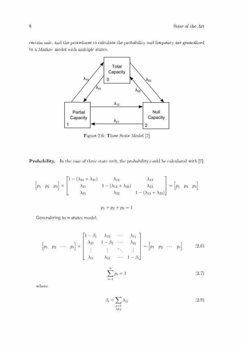
8 State of the Art

certain unit, and the procedures to calculate the probability and frequency are generalized

to a Markov model with multiple states.

Null Capacity

0

1 2

Total Capacity

Partial Capacity

λ10

λ20

λ02

λ12

λ21

λ01

Figure 2.6: Three State Model [7]

Probability. In the case of three state unit, the probability could be calculated with [7]:

[p1 p2 p3

]×

1− (λ21 + λ31) λ12 λ13

λ21 1− (λ12 + λ32) λ23

λ31 λ32 1− (λ13 + λ23)

=[p1 p2 p3

]

p1 + p2 + p3 = 1

Generalizing to n states model:

[p1 p2 · · · pi

]×

1− β1 λ12 · · · λ1j

λ21 1− β2 · · · λ2j...

.... . .

...

λi1 λi2 · · · 1− βi

=[p1 p2 · · · pi

](2.6)

n∑i=1

pi = 1 (2.7)

where

βi =∑j=1i 6=j

λij (2.8)

2.2 General Concepts of Generation Systems Reliability Adequacy Assessment 9

Frequency. Given the probabilities of each state and the respective transitions rates,

the frequency of the system is in the state s is [1]:

f(s) = p(s)λd(s) =∑v

p(v)λvs (2.9)

where

• λd(s) - Transition rate from state s.

• v - State that transits to s.

• p(v) - Probability of state v.

• λvs - Transition rate from state v to s.

Therefore, the frequency of the system is in the state s is equal to the sum of proba-

bilities of being in a state which is not s and there is a transition to the s state.

2.2.2 Generation Reliability indices

Methods based on the Probabilistic Approach usually culminate in the calculation/estimation

or in the probability distribution of a set of reliability indices. Usually analytical methods

could not achieve the analysis of the probability distribution, so, simulation methodologies

should be applied. The reliability indices are expressed in value per year and are brie�y

addressed as follows (indices for HL1 studies) [3].

• Loss of Load Probability (LOLP) � represents the probability of occurring a load

curtailment event in a given time period (T) (normally a year). Dimensionless index;

• Loss of Load Expectation (LOLE) � represents the average number of days or hours

in a given time period (normally a year) in which the load value is expected to exceed

the available system capacity. Expressed in timebase/T;

LOLE = LOLP × T (2.10)

• Expected Power Not Supplied (EPNS) � represents the expected power not supplied

by the generating system due to load demand exceeding the available generating

capacity. Expressed in MW/T;

• Expected Energy Not Supplied (EENS) � represents the expected energy not supplied

by the generating system due to load demand exceeding the available generating

capacity. Expressed in MWh/T;

EENS = EPNS × T (2.11)

10 State of the Art

• Loss of Load Frequency (LOLF) � represents the expected frequency of encountering

a de�ciency. Expressed in occurrences/T;

• Loss of Load Duration (LOLD) � represents the average duration of an interruption

of power supply. Expressed in timebase/disturbance;

LOLD =LOLP

LOLF(2.12)

• Mean Time Between Failures (MTBF) - represents the stationary time between fail-

ures;

MTBF =1

LOLF(2.13)

In the literature, it is accepted that analytical methodologies just could provide an

estimation of the mean value of the indices. In reference [8], It is said that the sequential

Monte Carlo simulation is the only realistic option available to investigate the distributional

aspects associated with system index mean values. Also, in reference [9] the same idea is

emphasized: the sequential MCS is the natural tool to simulate chronological aspects. It

is not only able to assess the usual reliability indices, but also their respective probability

distributions.

2.3 Analytical Approach for Reliability Evaluation

Analytical approaches have limitations to reliability assessment studies due to the need of

formulating multiple simpli�cations on complex systems. Among the analytical methods,

the most relevant (given the historical relevance and extreme simplicity that allow the

best performances) are the Recursive Method, Frequency and Duration Method (F&D)

and Fast Fourier Transform Convolution Method (FFT), all of which considering the State

Space representation (like any other purely based Analytical Method).

Starting with the Recursive Method, being the easiest to implement, it fails to obtain

important information related to the system behavior, such as frequency and duration

of interruptions. However, the Frequency and Duration method (F&D) can complement

such issues if implemented additionally. However, these methods require too much com-

putational time when analyzing Power Systems of considerable dimension, as is the case

of real Power Systems. Bearing such concerns in mind, the Convolution (FFT [10]) and

Gram-Charlier Expansion [11] methods were developed. These methods use the concept

of unavailability, which is the probability of �nding the generation unit out of service, to

construct the Capacity Outage Probability Table.

2.3 Analytical Approach for Reliability Evaluation 11

2.3.1 Recursive Method and F&D Method

The Recursive Method relies on the notion of unavailability/availability, related to the

probability of discovering the generator unit out/in service, to build recursively the Capac-

ity Outage Probability Table. Due to its straightforwardness, the two-state homogeneous

Markov model is broadly employed to represent the operation cycle of the generator unit,

with its unavailability being known as Forced Outage Rate (FOR).

As an example, to fully portray generation system reliability of a generation unit the

only information required is its mean time to failure and its mean time to repair. This

information can be acquired from the analysis of the behavior history of the unit being

considered. These types of studies can comprise even more exhaustive models to represent

the unit's exact operating settings, similar to peaking service [6, 12].

In order to to minimize computational e�ort in large-scale systems, it is usual to trun-

cate the Capacity Outage Probability Table (COPT), reducing the discrete probability of

a failure event. Equation 2.14 illustrates how to calculate the accumulated probability of

a certain state of the COPT [7].

P (y) =

n∑j=1

p′(y − cj)p(cj) (2.14)

where P (y) is the accumulated probability of state's capacity out of service y, p′(y− cj) iszero when y is bigger then individual state cj , and n is the number of individual states.

Regarding the F&D method, it is meant to supply reliability indices that demonstrate

the system failure occurrence frequency and the expected duration for such outages, which

are seen as the aforementioned method key advantages. Its major disadvantage compared

to the Recursive Method is its slightly more complex conceptuality due to the concepts of

frequency and state transition. It includes a Generation Model Table (GMT) described as

shown in equation below [7].

GMT = {cG; pg; fG} (2.15)

where cG, pG and fG are the capacity, probability and frequency respectively of each state.

In summary, the F&D methods compute the transition rates connecting the di�erent

states that comprise the composed Markov model. Similarly to the recursive method, the

load model is convoluted with the recursively built Capacity Outage Probability Table in

order to obtain the reliability indices. The load uncertainty can as well be included in the

F&D methods. References [6] and [10] provide the theoretical basis for the aforementioned

methods. For unbalanced systems as to balanced ones, the transition rates, and cumulated

frequency are obtained as follows.

p(y) =n∑j=1

p′(y − cj)p(cj) (2.16)

12 State of the Art

f+(y) =

n∑j=1

[p′(y − cj)f+(cj) + p(cj)f′+(y − cj)] (2.17)

f−(y) =n∑j=1

[p′(y − cj)f−(cj) + p(cj)f′−(y − cj)] (2.18)

f c(y) =n∑j=1

[p′(y − cj)f c(cj) + p(cj)f′c(y − cj)] (2.19)

λ+(y) =f+(y)

p(y)(2.20)

λ−(y) =f−(y)

p(y)(2.21)

The recursive way to obtain the accumulated states of a frequency unbalanced system

may be done by [7]:

PN = PN+1 + piFN = FN+1 + pi(λNi − λAi ) + f ci (2.22)

where

• PN � Probability of cumulative state after addition of state i.

• PN+1 � Probability of cumulative state before addition of state i.

• FN � Frequency of cumulative state after addition of state i.

• FN+1 � Frequency of cumulative state before addition of state i

• pi � Probability of state i.

• λNi � Transition rate from state i to all individual state not accumulated.

• λAi � Transition rate from state i to all individual state already accumulated.

• f ci =∑i∈J

(piλij − pjλji) � Frequency correction factor and J is the set all individual

states already accumulated before addition of i.

2.3.2 FFT Convolution

In both references [13] and [10] the FFT method is explained. Such method was developed

with the intent of lessening the computational e�ort required by states combination. Thus,

a convolution process based on the Fast Fourier Transform is applied with the purpose of

acquiring the Capacity Outage Probability and Frequency Table. A frequency domain rep-

resentation is used for the convolution operation, in which the multiplication of the impulses

is processed individually, converting afterwards in return to the time domain. Indeed, the

2.3 Analytical Approach for Reliability Evaluation 13

frequency domain possesses considerable amount of null points, rendering a mathematic

procedure less time consuming in comparison with the Fourier Transform Method. Such

methodology promotes the individual addition/reduction of generation capacity, with the

convolution of their probabilities and frequencies as discrete impulses.

PGk = PGi ∗ PGj (2.23)

f+Gk = PGi ∗ f+Gj + PGj ∗ f+Gi (2.24)

f−Gk = PGi ∗ f−Gj + PGj ∗ f−Gi (2.25)

f cGk = PGi ∗ f cGj + PGj ∗ f cGi (2.26)

To employ FFT convolution based operation all units may have (depending on FFT

algorithm) the same number of states (2n) with the same interval between each states. As

a result, �xed impulses with constant frequency intervals are de�ned previously to the con-

volution procedure. Since this situation are an uncommon reality, thus weighted-averaging

method should be implemented. Therefore, previously to the convolution procedure, it is

necessary to determine how many states the �nal solution will have.

Let Tij be the system's capacities interval, and Ti and Tj the di�erence between the

higher and lower capacities from units i and j (Ti = ximax − ximin). Then, Tij is given by

Tij = (ximax + xjmax)− (ximin + xjmin) (2.27)

If Nij is the number of necessary points to represent the interval Tij , knowing that 2M

points are required, so, Nij could be deduced as follows.

N ′ij = 2M (Tij/T ), T =L∑i=1

Ti (2.28)

M ′ij = log2(N′ij) (2.29)

Mij = int(M ′ij) + 1 (2.30)

Nij = 2Mij (2.31)

The computational e�ort may be reduce if units are included in ascending order of

capacity. Given a point which is comprehended in a predetermined interval, probability

and frequency are linearly divided among the upper/down points of the limit through an

14 State of the Art

weighted-averaging method (Figure 2.7).

Cn

Ci

∆

Cm

∆1 ∆2

Figure 2.7: Weighted-averaging sharing process [13].

If m and n are weighted-averaging states (where state capacity of m is bigger than n)

the division of state i through both is given by [7].

pmi = pici − cncm − cn

= pi∆2

∆(2.32)

pni = picm − cicm − cn

= pi∆1

∆(2.33)

λ+mi= λ+ni

= λ+i (2.34)

λ−mi= λ−ni

= λ−i (2.35)

When n represents a state with null capacity or m maximum capacity λ+mi= 0 and

λ−ni= 0.

f±mi= pmiλ

±mi

=∆2

∆piλ±i =

∆2

∆f±i (2.36)

f±ni= pniλ

±ni

=∆1

∆piλ±i =

∆1

∆f±i (2.37)

The states with equal capacities m and mi, n and ni are combined respectively with r

and s:

cr = cm (2.38)

2.3 Analytical Approach for Reliability Evaluation 15

cs = cn (2.39)

pr = pm + pi∆2

∆(2.40)

ps = pn + pi∆1

∆(2.41)

f±r = f±m + f±mi(2.42)

f±s = f±n + f±ni(2.43)

In the same way to frequency correction factor:

f cmi=

∆2

∆f ci (2.44)

f cni=

∆1

∆f ci (2.45)

f cr = f cm + f cmi(2.46)

f cs = f cn + f cni(2.47)

More than prepare the array of points to convolve, the weighted-averaging method

could reduce the complexity of the global system, and a correspondent improvement of

computational e�ciency can be performed through the usage of the procedure presented

in [13], which can be perceived as a method that dynamically addresses the domain, con-

sidering that the quantity of points enlarges in relation to the quotient of the generation

capacity observed for each instant.

2.3.3 Load Model

Figure 2.8 presents three simpli�ed models of load. One considers the peak load to all load

cycle, so, a constant load is compared to the generation model and then the index LOLP is

determined. This method introduce excessive errors leading to a too conservative approach.

A less conservative methodology is the linearization of load diagram, which can re�ect the

variation on load through the year, but could not capture the frequency, since, transitions

disappears with the linearization process. Hence, the most common representation to index

evaluations is the hourly modeled load, that is composed by load constant steps through

16 State of the Art

Figure 2.8: Single curve load representations [14].

the complete period. In this approach, it is possible to build a load model with the same

parameters as the generation model using equation 2.48 [10].

LMT = {cL; pL; fL} (2.48)

where LMT is the Load Model Table and cL, pL, fL are the capacity, probability and

frequency respectively of each load state.

2.4 Simulation Methods

Over the past two decades, the �eld of computation has seen some decisive achievements in

the processes of improvement of simulation methods on di�erent applications. Monte Carlo

methods, which are statistically-based, were the �rst simulation methods to be widely

implemented. Using random variable sampling, it is possible to simulate the system's

behavior in regards to the reliability indices, and therefore to obtain an accurate estimation

of these indices [6].

About these matters, the System State Sampling (Non-Sequential Monte Carlo Simu-

lation - NSMCS) simulation consists in sampling system states independently of the time

periods in which they occur. The System State Transition Sampling (Sequential Monte

Carlo Simulation - SMCS) simulation, on the other hand, consists of sampling the next

system state thus advancing variable time periods per iteration, rather than �xed time

intervals. While NSMCS assumes the system's State Space Representation, the SMCS

assumes the chronological representation.

Unlike the analytical method, which tries to assess all the system states contained

in state space, or approximations of such, through mathematical models and equations,

simulation methods rely on a set of simulations representing the actual system behavior

to reach the reliability indices.

2.4 Simulation Methods 17

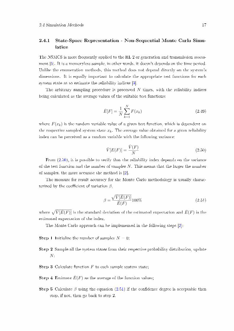
2.4.1 State-Space Representation - Non-Sequential Monte Carlo Simu-

lation

The NSMCS is more frequently applied to the HL 2 or generation and transmission assess-

ment [5]. It is a memoryless sample, in other words, it doesn't depends on the time period.

Unlike the enumeration methods, this method does not depend directly on the system's

dimensions. It is equally important to calculate the appropriate test functions for each

system state as to estimate the reliability indices [3].

The arbitrary sampling procedure is processed N times, with the reliability indices

being calculated as the average values of the suitable test functions:

E[F ] =1

N

N∑k=1

F (xk) (2.49)

where F (xk) is the random variable value of a given test function, which is dependent on

the respective sampled system state xk. The average value obtained for a given reliability

index can be perceived as a random variable with the following variance:

V [E(F )] =V (F )

N(2.50)

From (2.50), it is possible to verify that the reliability index depends on the variance

of the test function and the number of samples N . This means that the larger the number

of samples, the more accurate the method is [2].

The measure for result accuracy for the Monte Carlo methodology is usually charac-

terized by the coe�cient of variation β,

β =

√V [E(F )]

E(F )100% (2.51)

where√V [E(F )] is the standard deviation of the estimated expectation and E(F ) is the

estimated expectation of the index.

The Monte Carlo approach can be implemented in the following steps [2]:

Step 1 Initialize the number of samples N = 0;

Step 2 Sample all the system states from their respective probability distribution, update

N ;

Step 3 Calculate function F to each sample system state;

Step 4 Estimate E(F ) as the average of the function values;

Step 5 Calculate β using the equation (2.51) if the con�dence degree is acceptable then

stop, if not, then go back to step 2.

18 State of the Art

The NSMCS possesses a disadvantage associated with its inability to fully address the

system's chronological characteristics. On the other hand, it is able to assess the reliability

indices in less computational time and with less memory storage when comparing it with

SMCS methods.

2.4.2 State Space Representation - Population Based Methods

Both Population Based (PB) and NSMCS methods simulate system behaviour in the State

Space Representation, so, it is not able to represent the chronological behaviour of the sys-

tem, hence, it does not bene�t from a complete representation of the system, as Sequential

Monte Carlo Simulation(next described).

PB methods promotes a search at the State Space Representation with the intend to

capture relevant states, for a faster evaluation of the indices. For reliability assessment

proposes the sates of interest are the failure states, therefore, PB could �nd those states

be the de�nition as a prede�ned threshold.

Depending on the method applied, de�nitions of the threshold may di�er. In PB

methods, a given reliability index is given by its estimate, F , obtained as follows [15]:

F =∑i∈D

piFi (2.52)

where D is the set of sampled failure system states, pi is the probability of failure system

state x, Fi is the value of the desired index test function related to state x, and D is the

set containing the states found, with D contained in the State Space (i.e. X).

As Population-Based is not in the scope of this thesis, only a summarise of PB tech-

niques applied in the resolution of the Power System Reliability Assessment are presented:

• Genetic Algorithms-based methods [16] [17]

• Swarm Intelligence (SI)-based methods [18] [19].

• Hybrid EA/SI EPSO technique [15].

PB methods do not follow the statistical theorems for sampling, with both advantages

and disadvantages. On the upside, it implies that they are able to visit the states of interest

must faster than other methods (e.g.Statistically Based Methods, Analytical Methods, etc),

acquiring acceptable reliability indices earlier in the estimation process. The downside is

that its non-statistical methods take away the statistical traceability, unable to de�ne an

interval of con�dence related to the solution obtained.

2.4.3 Sequential Monte Carlo Simulation

The SMCS uses the component's state duration distribution functions. Consider a single

component model where a component has two states, an operating state and a repair state.

2.4 Simulation Methods 19

These stochastic states are associated with the Mean Time To Failure (MTTF) and Mean

Time To Repair (MTTR), which are assumed to be exponentially distributed.

For the SMCS approach, the estimation of reliability indices is obtained as follows [20]:

E[F ] =1

NY

NY∑n=1

F (yn) (2.53)

where NY is the number of simulated years and yk is the sequence of system states in year

k.

The sequential approach can be summarized in the following steps:

Step 1 Initiate all the component state. Commonly it is assumed that all the components

are in the state UP or operational;

Step 2 Sample the duration of each component in the actual state. If using a exponential

distribution for the state duration, then the duration of the state is calculated as

Ti = − 1

λiln(Ui) (2.54)

where Ui is a uniformly distributed random number between [0, 1], i stands for the

component number.

Step 3 Repeat the step 2 each time span, in this case yearly, and record the results of

each duration sampled for all components;

Step 4 In order to obtain yearly reliability indices, calculate the test function F (yn) over

the accumulated values;

Step 5 Estimate the expected mean values of the yearly indices as the average over the

yearly results for each simulated sequence yn;

Step 6 The stop criterion is also based on the relative uncertainty of the estimates. There-

fore, calculate β (coe�cient of variation) using (2.51);

Step 7 End methodological procedure if the desired degree of con�dence is achieved. If

not return to step 2.

The advantages of the SMCS are:

• It can easily calculate the actual frequency index;

• It considers any state duration distribution, exponential or non-exponential distribu-

tions;

• It can calculate the statistical probability distributions of the reliability indices in

addition to their expected value.

Figure 2.9 represents a single component system's chronological transition process.

20 State of the Art

Figure 2.9: Single component system chronological transition process

2.5 Hybrid Approaches

Hybrid methods were developed to improve on some of the characteristics of classic meth-

ods, and since simulation methodologies already have a complete and realistic approach,

the main objective is to speci�cally improve performance. Even so, the reduction of com-

putational e�ort originates an almost unavoidable loss of information and its quality.

In this thesis, the classi�cation and de�nition of the classic Analytical/Simulation inter-

pretation of �Hybrid Method� will be taken one step further, namely through the combined

use of various algorithmic mechanisms. Three Monte Carlo-based Methods considered to

be Simulation/Simulation hybrids and two Cross-Entropy/Monte Carlo-based methods

considered to be conceptual hybrids are presented as cases of interest.

2.5.1 Analytical/Simulation Methods

Analytical/Simulation type of hybrid approach relies on both simulation and analytical

features in a uni�ed methodology, in order to retain the advantages of both methodologies.

An example of such methodological application can be observed in reference [21], where it

is employed to large hydrothermal generating systems. Monte Carlo methodology, though,

lacks in time e�ciency because of its elevated computational executing time. Hence, the

method present in the aforementioned reference merges the Monte Carlo methodology,

through which the energy states are acquired, and the Analytical methodology, through

which the reliability indices are calculated.

Reference [22] presents an alternative hybrid method still using an Analytical/Simulation

scheme, in which the recursive method is used to incorporate wind generation and hydro

depletion through its hourly usage over the timespan of a year.

Further analytical/simulation hybrid methodology is proposed in [23]. The decoupling

of generation and load subsets are introduced in order to separate stochastic capacities

(both generation and load) and time-dependant capacities. The �rst subset is processed in

an analytical manner and the time-dependent subset is evaluated according to the chrono-

logical steps used by SMCS. This method is the base for this thesis and will be detailed in

chapter 3.

2.5 Hybrid Approaches 21

2.5.2 Analytical/Statistical Methods - Pseudo�Sequential Monte Carlo

Methods

Pseudo-Sequential Monte Carlo Method [24] combines the state system sampling of the

NSMCS with the chronology simulation of the SMCS, processing only the failure sequences.

Prior to the application of the method, a considerable amount of yearly sequences is sim-

ulated using a similar process to the one used in SMCS. A small di�erence occurs on

Combined Pseudo-Sequential and State Transition Method [25],sequential simulation is

processed through System State Transition Sampling, which lead to a less computing time

and a loss of capture some chronological events.

A di�erent load model (Multi-Level Non-Aggregate Markov Load Model) is able to

restore the chronological aspect and is implemented in Pseudo-Chonological Simulation

with Time Varying Loads Method [26].

The purpose of this approach is to use the non-sequential method to select the failures

states of the system, and the sequential approach is only used when there is a complete

interruption of the system. The pseudo-sequential Monte Carlo simulation is described

with detail in [26].

2.5.3 Optimization/Simulation Methods - Cross-Entropy based Monte

Carlo Methods

Despite being one the most robust tools for Power System analysis, especially for large

Systems, the MC methods retains considerable di�culties in the probing process of very

rare events.

In order to suppress the aforementioned problem, several reduction techniques have

already been applied to power systems, with some presenting better results than orders

in what regards real power systems [27]. Despite such e�orts, rarity events were still a

problem deserving little discussion in reliability related literature.

Recent developments in such area are related to the Cross-Entropy (Kullback-Leibler)

distance concept [27], which serves as an optimization algorithm for the selection of dis-

torted parameters used in IS. The main idea is to make rare events occur more often by

substituting original test function f(.) of a given reliability index (in the IS terminology

referred as mass function) by other density function fopt(.)(also referred as optimal distor-

tion), thus obtaining variance reduction. The innovation brought by referred [27] is the

iterative process, i.e. Cross-Entropy, presented to reduce the �distance� between both mass

functions and its application in reliability assessment indices calculation, also presenting

an adapted notation of the standard NSMCS method [27]. The distortion is applied to

unit generating availabilities. Resultant Cross Entropy and Monte Carlo-based method

can be considered as a hybrid between both concepts.

22 State of the Art

The Cross-Entropy concept is further applied to the SMCS method in [28]. A slightly

di�erent optimization process (still based on Cross Entropy Method) is used, but distortion

is applied only to the failure rates of components.

Chapter 3

A Hybrid Approach for Generating

Systems Reliability Evaluation.

3.1 Analytical Evaluation � FFT convolution

This thesis proposes to obtain a probability distribution of LOLE using analytical methods.

Because of its proven e�ciency, the convolution process is the unquestionable choice for the

developed work. For didactic proposes, as to identify some aspects that are not, arguably,

clearly explained in the literature, the algorithm was modi�ed and coded from the scratch

with object-oriented paradigm.

Therefore, in this section the �ow chart and the class diagram of the algorithm is pre-

sented, as well as some modi�cation in the FFT approach (see section 2.3). The main

di�erence lies in the way that the impulses are split into impulses array, that are pre-

pared to convolve. Then, it is categorically demonstrated the relation between incremental

frequency and transition frequencies (f+, f− and f c).

To explain all the methodology, a three thermal generators system with twelve hours

load cycle was applied.

3.1.1 Generation Model Table (GMT)

To reliability evaluation, the data necessary to characterize the generator is their static

state transitions rates and of course the capacity of each state. Most of this information

come from historical data collection. Therefore, all the remainder variables are obtained

by mathematical formulation.

3.1.1.1 Thermal Generation

For reliability assessment, thermal units are well behaved technologies since its available

power does not depends on external factors. Thus, for only thermal systems the method-

ology is well known and studied as explained in section 2.3.

23

24 A Hybrid Approach for Generating Systems Reliability Evaluation.

It is important to emphasize that the convolution methodology is extremely fast and

reliable aiming at obtaining the GMT table. Next, it is presented a step by step example

for the convolution methodology of a three generators system.

Example. In Table 3.1, it is shown the system generator's data.

Table 3.1: Three Generators data

Unit Capacity(MW) MTTR MTTF

1 25 2 100

2 25 2 100

3 50 2 100

It can be observed that all units are modelled with a two state model. Thus, it is

frequency balanced and equations 2.1 to 2.5 can be used producing the values shown in

Table 3.2. Notice that instead of frequency of encounter the state, it is used the frequency

to leave the state, that is divided in frequency to exit to states with more capacity (f+)

and frequency to exit to states with smaller capacity (f−), however, the arithmetic are

exactly the same. Since all units have the same parameters, only the values for unit 1 are

presented.

Table 3.2: FOR and frequency

State Capacity(MW) Probability f+ f−

0 0 0.0196 0.0098 0

1 25 0.9804 0 0.0098

Now, there is the condition to start the convolution process. Two units convolution are

illustrated in Figure 3.1. Notice that the amplitude of the probability Dirac in the image

are not proportional.

0.0196

0.9804

0 25P(MW)

*0.0196

0.9804

0 25P(MW)

=

0.0004

0.0384

0 25P(MW)

50

0.9612

Figure 3.1: Probability convolution unit 1 and 2

All convolution process for this example are explicated below.

pC0 = 0.01962 = 0.0004

3.1 Analytical Evaluation � FFT convolution 25

pC25 = (0.0196× 0.9804)× 2 = 0.0384

pC50 = 0.98042 = 0.9612

To obtain f+, the convolution process is shown in Figure 3.2 and the procedure to

calculate f− is exactly the same. Next, it is presented the calculations.

0.0196

0.9804

0 25P(MW)

*0.0098

0 25P(MW)

=

0.0003

0.0192

0 25P(MW)

50

+0.0196

0.9804

0 25P(MW)

*0.0098

0 25P(MW)

Figure 3.2: f+ convolution unit 1 and 2

f+C0= 0.0196× 0.0098 + 0.0196× 0.0098 = 0.0003

f+C25= 0.9804× 0.0098 + 0.9804× 0.0098 = 0.0192

f+C50= 0

The frequency f+ of the C50 state is 0 as it should be since there is no state with more

capacity obtained from the convolution of this two units. Hence, a built GMT table for

this example is shown in Table 3.3.

Table 3.3: GMT for the three generators system.

State Load(MW) Probability f+(o/h) f−(o/h)

1 0 7.54× 10−6 1.13× 10−5 0

2 25 7.54× 10−4 7.54× 10−4 7.54× 10−6

3 50 0.0192 0.0098 3.81× 10−4

4 75 0.0377 0.0188 7.54× 10−4

5 100 0.9423 0 0.0283

26 A Hybrid Approach for Generating Systems Reliability Evaluation.

3.1.1.2 Hydro Generation

The main di�erences between thermal generation and hydro generation from the reliability

evaluation view is essentially that, hydro generation does not depends only on generator

capacities to provide its full capacity. The power generation capacity also depends on

the resource availability (water), thus some changes to the presented thermal modeling

technique must be introduced.

In this work, the approach to deal with this conditionality is to a�ect linearly the

maximum capacity of each generator with the resource availability. Therefore, if C is the

hydro plant maximum capacity and r the resource availability, then the a�ected capacity

can be obtained by

Caffected = C × r (3.1)

The data utilized in this thesis has monthly water reserve availability, so in each month

every hydro plant must be combined with the thermal GMT to obtain a new GMT with

hydro generation.

3.1.2 Load Model Table (LMT)

For this thesis the load model representation used to evaluate reliability indices is given

by a constant load value to each step of a load diagram. A complete load cycle is named

period. Typically the period for real case studies is a complete year, i.e 8760 steps of load.

With the load cycle for a certain period (T ), it is now possible to obtain the transition

rates and the probability of each load state. Therefore, the load state probability and the

transition matrix could be calculated with equation 3.2 and 3.3 respectively, where pLi is

the probability of load state i, tLi is the total time of occurrences of the same state and

nLi,Lj is the number of transition from state Li to state Lj .pL1

pL2

...

pLi

=

tL1TtL2T...tLiT

(3.2)

1− β1 λ12 · · · λ1j

λ21 1− β2 · · · λ2j...

.... . .

...

λi1 λi2 · · · 1− βi

=

1− β1

nL1,L2tL1

· · ·nL1,Lj

tL1nL2,L1tL2

1− β2 · · ·nL2,Lj

tL2...

.... . .

...nLi,L1tLi

nLi,L2tLi

· · · 1− βi

(3.3)

where βi is calculated as in equation 2.8.

Using probability vector and transition matrix, the construction of LMC table could

be accomplish, using equations (2.16 to 2.21).

3.1 Analytical Evaluation � FFT convolution 27

Example. For the same model this methodology will be implemented. To do that, the

twelve hours load cycle is presented in Figure 3.3.

60

50

25

P(MW)

t(h)1 2 3 4 5 6 7 8 9 10 11 120

Figure 3.3: Twelve hours load cycle

In this diagram, three load states were identi�ed L1 (25 MW), L2 (50 MW), L3 (60MW)

and can be expressed as a state transition diagram similar to the one shown in Figure 2.5,

as illustrated in Figure 3.4. This is a three state model, therefore, it is not frequency

balanced so a frequency correction factor must be applied. The probability vector is:

60 MW

L1

L2 L3

25 MW

50 MW

λ21

λ31

λ23

λ32

λ12

Figure 3.4: Transition diagram from twelve hours load cycle.

pL1

pL2

pL3

=

412412412

=

131313

So the occurrence probability of each state is equal and have the value of 1

3 . Then the

transition matrix is calculated:1− β1 λ12 λ13

λ21 1− β2 λ23

λ31 λ32 1− β3

=

1− (14 + 14) 2

4 014 1− (24 + 1

4) 24

14

14 1− 1

4

28 A Hybrid Approach for Generating Systems Reliability Evaluation.

Frequency is given in occurrences per hour(o/h), thus, the frequency of L2 is:

f+L2 = pL2λ23 =1

3× 2

4= 1.667(o/h)

f−L2 = pL2λ21 =1

3× 1

4= 0.083(o/h)

f cL2 = pL2λ23 − pL1λ32 =1

3× 2

4− 1

3× 1

4= 0.083(o/h)

As it was mentioned before, this is not a frequency balanced model. Table 3.4 shows

the LMT for this example.

Table 3.4: LMT for twelve hours load cycle

State Load(MW) f+(o/h) f−(o/h) fc(o/h)

1 25 1.667 0 0

2 50 1.667 0.083 0.083

3 60 0 1.667 0

3.1.2.1 Wind Integration

The wind generation is typically obtained through wind turbines that are agglomerated in

wind farms/parks scattered by a certain territory. Due to this particular characteristic and

intrinsic speci�cations, wind generation power is a�ected by the wind �ow of a particular

zone. For static reliability assessment purposes, a wind farm could be characterized as

a single power plant with available power equal to the sum of each wind turbine power,

a�ected by the wind �ow availability. The data for wind availability comes from the

historical data collected. Thus, despite the wind park being considered a power plant,

failure rates may not be necessary since the historical data intrinsically have failure and

repair information.

In the scope of this thesis, the wind generation was integrated directly in the load value.

This means that for each hour and respective load, all the wind generation are a�ected

linearly by wind capacity also for the respective hour, being directly reduced in the load

value. The mathematical formulation can be written as shown below.

Let Pwi be the wind generation capacity of the i-th wind farm and Aih be the wind

pro�le factor of wind farm i at hour h. Then, the total wind generation at hour h is given

by

Pwh=

n∑i=1

Pwi ×Aih (3.4)

3.1 Analytical Evaluation � FFT convolution 29

So, integrating the wind generation with load, it results that

Lwh= Lh − Pwh

(3.5)

Then all the procedure presented in section 3.1.2 can be done normally. Notice that

only the load value is a�ected, neither probability or transition frequency change with wind

integration.

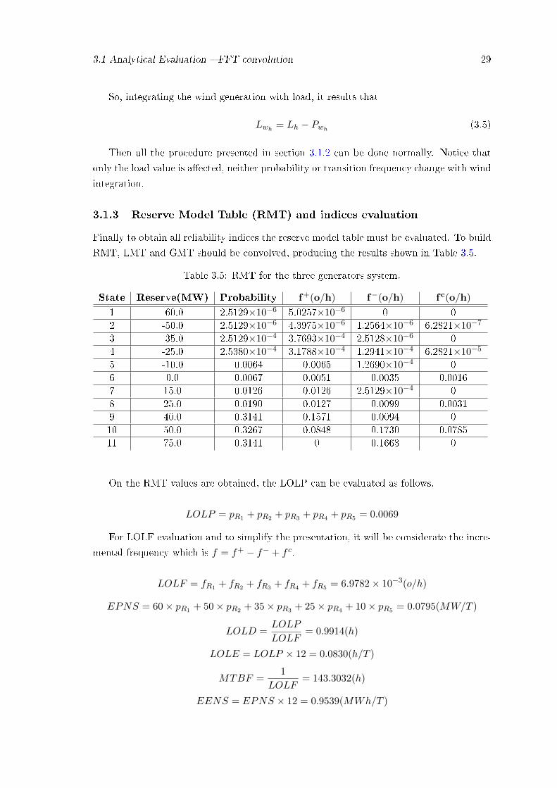
3.1.3 Reserve Model Table (RMT) and indices evaluation

Finally to obtain all reliability indices the reserve model table must be evaluated. To build

RMT, LMT and GMT should be convolved, producing the results shown in Table 3.5.

Table 3.5: RMT for the three generators system.

State Reserve(MW) Probability f+(o/h) f−(o/h) fc(o/h)

1 -60.0 2.5129×10−6 5.0257×10−6 0 0

2 -50.0 2.5129×10−6 4.3975×10−6 1.2564×10−6 6.2821×10−7

3 -35.0 2.5129×10−4 3.7693×10−4 2.5128×10−6 0

4 -25.0 2.5380×10−4 3.1788×10−4 1.2941×10−4 6.2821×10−5

5 -10.0 0.0064 0.0065 1.2690×10−4 0

6 0.0 0.0067 0.0051 0.0035 0.0016

7 15.0 0.0126 0.0126 2.5129×10−4 0

8 25.0 0.0190 0.0127 0.0099 0.0031

9 40.0 0.3141 0.1571 0.0094 0

10 50.0 0.3267 0.0848 0.1730 0.0785

11 75.0 0.3141 0 0.1663 0

On the RMT values are obtained, the LOLP can be evaluated as follows.

LOLP = pR1 + pR2 + pR3 + pR4 + pR5 = 0.0069

For LOLF evaluation and to simplify the presentation, it will be considerate the incre-

mental frequency which is f = f+ − f− + f c.

LOLF = fR1 + fR2 + fR3 + fR4 + fR5 = 6.9782× 10−3(o/h)

EPNS = 60× pR1 + 50× pR2 + 35× pR3 + 25× pR4 + 10× pR5 = 0.0795(MW/T )

LOLD =LOLP

LOLF= 0.9914(h)

LOLE = LOLP × 12 = 0.0830(h/T )

MTBF =1

LOLF= 143.3032(h)

EENS = EPNS × 12 = 0.9539(MWh/T )

30 A Hybrid Approach for Generating Systems Reliability Evaluation.

3.1.4 Rounding Technique

To round the incremental frequency of a speci�c state from a unit, in the case that the

states of the unit are not multiple of the rounded increment, is would be simple to split the

frequency proportionally to the state capacity to the neighbor states. Nevertheless, this

method is not always realistic. For example, let us consider a generator with two states

whose capacities are 0 and 15 MW, the probabilities are 0.02 and 0.98, the frequencies f+

are 0.3 and 0, and a rounding increment of 10 MW to build the generating capacity model.

Considering that it is needed four states to convolve that unit, since, 2n states are required

to convolve. Then, the �nal states are 0, 10, 20 and 30, therefore, it is necessary to split

the probability and the incremental frequency.

In the case we split proportionally, results obtained are presented in Table 3.6.

Table 3.6: Proportional Split

C(MW) 0 10 20 30

p 0.02 0.49 0.49 0

f+ 0.3 0 0 0

Although this is not realistic, in the way that the new state of 10 MW have no frequency

to transit to a state with large capacity, there is indeed a state with probability di�erent

from 0 with larger capacity. This means that there are no possibilities to transit from state

10 to 20, even knowing that state 20 have a certain probability to occurs.

The solution presented is not to slip the last state but just equal the probability and

the incremental frequency of the pre-rounded state to the one which the state capacity is

near to the pre-rounded state capacity. In Table 3.7 are given the results for the same

example.

Table 3.7: Modi�ed Split

C(MW) 0 10 20 30

p 0.02 0.98 0 0

f+ 0.3 0 0 0

This method generate higher probability to states that does not exist, and if the round-

ing increment is large, it can change the value of the indices. One possible solution is to

make rounding increment smaller as possible, or if possible, the maximum common divider

of all pre-rounded states. For real cases this value can be too small, which leads to an

increase of computational e�ort.

Another remark that is not well-explained in [7] is the fact that the rounding incre-

ment causes a deviation from the real system capacity from the obtained capacity by the

convolution process.

3.1 Analytical Evaluation � FFT convolution 31

3.1.5 Incremental Frequency Technique

The cumulative frequency given a certain state space, can be calculated by:

Fk = Fk+1 + fk (3.6)

where fk is the incremental frequency and Fk+1 is de cumulative frequency before adding

k state.

Supposing that S+k is the set of states not yet combined and S−k is the set of states

already combined. Typically, S+k is the set of states with large capacity and S−k the states

with smaller capacity.

If k is the state ready to be added, fk is given by:

fk =∑y

fky −∑z

fzk (3.7)

With y ∈ S+k and z ∈ S−k .

It is also known that fky = pk × λky and fzk = pz × λyk, so:

fk =∑y

pkλky −∑z

pzλzk (3.8)

If add and subtract fkz:

fk =∑y

pkλky −∑z

pzλzk +∑z

pkλkz −∑z

pkλkz (3.9)

Now if f+k =∑ypkλky, f

−k =

∑zpkλkz and f

ck =

∑zpkλkz −

∑zpzλzk, results:

fk = f+k − f−k + f ck (3.10)

Given a load diagram or a diagram of transitions between states from some kind of

generator, it is possible to calculate the transitions rates between those states using the

expressions presented behind.

The process to calculate incremental frequency is the one explained below:

1. Determinate the period of the load diagram (T).

2. Count the total times that each state appears in the diagram (tk).

3. Now it's possible to calculate the probability of state k: pk = tkT

4. Count the number of transitions between states from S−k and k , and transitions

between k and states from S+k , lets say that, nky and nzk denotes the number of

transitions from state k to states belonging to S+k and S−k , respectively.

32 A Hybrid Approach for Generating Systems Reliability Evaluation.

5. There are now conditions to calculate de transition rates λky and λzk:

λky =nkytk

(3.11)

In the same way:

λzk =nzktz

(3.12)

6. Now we can use the expression fk =∑ypkλky −

∑zpzλzk.

If the duration of every steps are equal in all diagram we can simplify the equation

above to:

fk =

∑ynky −

∑znzk

T(3.13)

Some times it is interesting to have more information about the transitions between

states. In this cases calculate f+k , f−k , f

ck can be interesting.

3.1.6 FFT Algorithm for Indices Evaluation

From the previous subsection, it was presented a particular example of the FFT method-

ology and how to get reliability indices for that speci�c example. In this subsection, it will

be developed a generic algorithm that could be applied to any input or system. Also, it

is presented validation results produced to guaranty that the further development are not

a�ected by a malformation of the algorithm or bugs committed in the codi�cation process.

The algorithm must be �exible enough to get partial evaluations (like monthly evalua-

tions), or to accept a large variety of inputs, such that for multi-state modeled units. Also,

the outputs must include as much information as possible.

3.1.6.1 Algorithm �owchart

A generic algorithm is presented in the �owchart shown in Figure 3.5. Due to the object

orientation codi�cation, the sequence may not be exactly as shown. For partial evaluation

this algorithm must be repeated as many times as necessary.

In the �owchart, the point A represents a partial end point if only GMT are necessary.

This point is particularly interested for this work to modify the hydro capacity without

losing the possibility to get partial indices, since in most available data the hydro resource

changes every month.

3.1 Analytical Evaluation � FFT convolution 33

Start

Read:Generation

and load data

Initialize GMT

Read unit

Create transitionmatrix for unit

Evaluatep, f+, f−, f c

Round statesof the unit

Convolve GMTwith the new unit

Every unitcombined?

Repeat dottedbox until all hy-dros are combined

Add hydro data

A

Identify load levels

Run load cycle andcompute p e fij

Add wind data

Evaluate load LMTf+, f−, f c

Convolve LMT withGMT and evaluatereliability indices

End

no

yes

Next hydro resource value

Figure 3.5: Flowchart of FFT algorithm

34 A Hybrid Approach for Generating Systems Reliability Evaluation.

3.1.6.2 IEEE RTS-79 Validation

As previously discussed, to proceed with the work the basis of all methodology must be

validate. Thus, the IEEE RTS-79 (see appendix A for system description) is the choice to

validate the program results, due to its good documentation and size.

In Table 3.8, it is shown comparative results with three methodologies presented in

IEEE articles. The �rst one is another FFT algorithm, then a Monte Carlo Simulation

and �nally the hybrid methodology Cross-Entropy Monte Carlo Simulation. The rounding

increment was 1 MW and state probability was truncated at 10−9. The error is evaluated

by equation 3.14. As it can be seen, the obtained error is quite small, thus all the results

are accurate and the algorithm is considered be valid.

Error(%) =|ResultToTest− TestResult|

TestResult(3.14)

Table 3.8: Results comparative for RTS-79

Method LOLE(h/year) LOLP LOLF(o/year) LOLE Error(%)

Algorithm Results 9.3551 1.0716×10−3 2.0142 -

FFT [10] 9.3332 1.0691×10−3 2.0073 0.23

MCS [29] 9.3280 1.0685×10−3 1.9996 0.29

CE-MCS [29] 9.3454 1.0705×10−3 2.0088 0.10

As already described, the algorithm is able to return partial indices. In Figure 3.6, it

is shown the evolution chart of the LOLE for the IEEE RTS-79 System and, in the Table

3.9, the value of these indices.

Figure 3.6: Monthly LOLE evaluation - RTS-79.

3.2 The Uni�ed Frequency Method 35

Table 3.9: Monthly indices evaluation RTS-79

Month LOLE(h/month) LOLP LOLF(o/month)

January 0.7859 0.0011 2.47×10−4

February 0.2245 3.46×10−4 8.31×10−5

March 0.0120 1.61×10−5 6.31×10−6

April 0.0400 5.55×10−5 1.97×10−5

May 0.6346 8.53×10−4 1.77×10−4

June 1.0416 0.0014 2.92×10−4

July 0.3128 4.20×10−4 8.77×10−5

August 0.0450 6.05×10−5 2.12×10−5

September 0.0191 2.65×10−5 9.62×10−6

October 0.1259 1.69×10−4 4.63×10−5

November 1.5294 0.0021 4.78×10−4

December 4.5911 0.0062 0.0013

3.2 The Uni�ed Frequency Method

As already discussed, the analytical approach is a quick and reliable method. Nevertheless,

for network operators and TSOs, it lacks on chronological information, and more impor-

tantly, it does not give a probability distribution of the indices. Therefore, it is not possible

to verify which indices are more likely to happen. Thus, in this section, it will be analyzed

how a chronological view can be an intrinsic information of the analytical approach or if

there are any connection between this two perspectives.

Then, it is presented result discussions, FFT convolution method is compared with

the methodology proposed. A canonical system with a three state modeled generator was

the system used to test. The description of the canonical systems may be analyzed in

Appendix A. The SMCS will not be tested, since, the multi-state unit of the canonical

system was not possible to simulate with the provided algorithm.

3.2.1 Analytical And Sequential Monte Carlo Simulation Comparison

To analyze the aspects of chronological simulation that are implicit in a state-space/analytical

view, a small system of one generator modeled with three states and a load cycle with just

three load points, named canonical system, will be used as shown in Figure 3.7.

In Figure 3.7c, it can be seen the representation of the state-spaces resultant from

Figure 3.7b and 3.7a. From the analytical point of view, this representation retains all

information that is necessary to obtain the indices. For example LOLP is simply the sum

of the probability of the states in failure side.

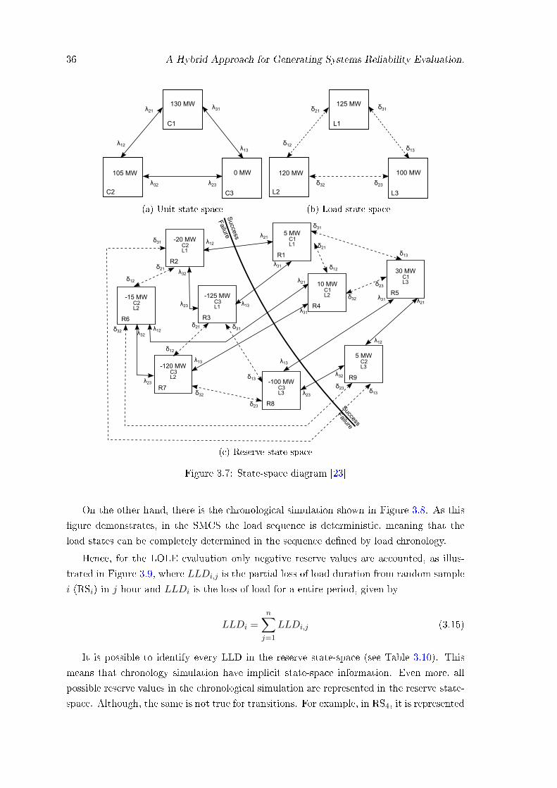
36 A Hybrid Approach for Generating Systems Reliability Evaluation.

0 MW

C1

C2 C3

130 MW

105 MW

λ21

λ12

λ32 λ23

λ31

λ13

(a) Unit state-space

100 MW

L1

L2 L3

125 MW

120 MW

δ21

δ12

δ32 δ23

δ31

δ13

(b) Load state-space

R1

5 MWC1L1

R4

10 MWC1L2 R5

30 MWC1L3

R9

5 MWC2L3

R2

-20 MWC2L1

R3

-125 MWC3L1

R8

-100 MWC3L3

R7

-120 MWC3L2

R6

-15 MWC2L2

λ12

λ21

λ31 δ12

δ21

δ31

λ21

λ31

δ32

δ23

δ13

λ21λ31

λ12

λ32

δ23 δ13λ23

λ13

δ13

δ23

δ32

λ13

δ12

δ21 δ31

λ13

λ23

λ32δ32

δ31

δ12

δ21

λ23

λ32

λ12S

uccess

Failure

Success

Failure

(c) Reserve state-space

Figure 3.7: State-space diagram [23]

On the other hand, there is the chronological simulation shown in Figure 3.8. As this

�gure demonstrates, in the SMCS the load sequence is deterministic, meaning that the

load states can be completely determined in the sequence de�ned by load chronology.

Hence, for the LOLE evaluation only negative reserve values are accounted, as illus-

trated in Figure 3.9, where LLDi,j is the partial loss of load duration from random sample

i (RSi) in j hour and LLDi is the loss of load for a entire period, given by

LLDi =n∑j=1

LLDi,j (3.15)

It is possible to identify every LLD in the reserve state-space (see Table 3.10). This

means that chronology simulation have implicit state-space information. Even more, all

possible reserve values in the chronological simulation are represented in the reserve state-

space. Although, the same is not true for transitions. For example, in RS4, it is represented

3.2 The Uni�ed Frequency Method 37

130

105

P(MW)

t(h)1 2 30

125

120

100

130

105

P(MW)

t(h)1 2 30

125

120

100

130

105

P(MW)

t(h)1 2 30

125

120

100

130

105

P(MW)

t(h)1 2 30

125

120

100

130

105

P(MW)

t(h)1 2 30

125

120

100

130

105

P(MW)

t(h)1 2 30

125

120

100

G

L

Random Sample 1 Random Sample 2 Random Sample 3

Random Sample 6Random Sample 5Random Sample 4

Figure 3.8: Unit state-space [23]

RS1 LLD1 = 0 h

RS2 LLD2= 2 h

RS3 LLD3 = 3 h

RS4 LLD4 = 1 h

RS5 LLD5 = 1.5 h

RS6 LLD6 = 0.5 h LLD6,2

LLD5,2

LLD4,2

LLD3,2

LLD2,2

LLD3,3

LLD2,1

LLD3,1

LLD5,1

T 1 2 3

Figure 3.9: Load state-space [23]

Table 3.10: Reserve State-Space and LLD relation

Reserve State LLD

R2 LLD2,1;LLD5,1

R3 LLD3,1

R6 LLD2,2;LLD4,2;LLD5,2;LLD6,2

R7 LLD3,2

R8 LLD3,3

a transition of load and capacity at the same time, which is not possible in the analytical

approach.

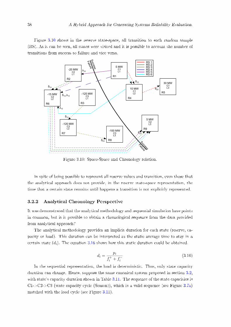
38 A Hybrid Approach for Generating Systems Reliability Evaluation.

Figure 3.10 shows in the reserve state-space, all transition to each random sample

(RS). As it can be seen, all states were visited and it is possible to account the number of

transitions from success to failure and vice versa.

R1

5 MWC1L1

R4

10 MWC1L2 R5

30 MWC1L3

R9

5 MWC2L3

R2

-20 MWC2L1

R3

-125 MWC3L1

R8

-100 MWC3L3

R7

-120 MWC3L2

R6

-15 MWC2L2

λ12

δ12

δ23

δ23

δ23

δ12

δ12

λ12

RS 1RS 2RS 3RS 4RS 5RS 6

Success

Failure

Success

Failure

δ12,λ12

Figure 3.10: Space-Space and Chronology relation.

In spite of being possible to represent all reserve values and transition, even those that

the analytical approach does not provide, in the reserve state-space representation, the

time that a certain state remains until happens a transition is not explicitly represented.

3.2.2 Analytical Chronology Perspective

It was demonstrated that the analytical methodology and sequential simulation have points

in common, but is it possible to obtain a chronological sequence from the data provided

from analytical approach?

The analytical methodology provides an implicit duration for each state (reserve, ca-

pacity or load). This duration can be interpreted as the static average time to stay in a

certain state (di). The equation 3.16 shows how this static duration could be obtained.

di =pi

f+i + f−i(3.16)

In the sequential representation, the load is deterministic. Thus, only state capacity

duration can change. Hence, suppose the same canonical system proposed in section 3.2,

with state's capacity duration shown in Table 3.11. The sequence of the state capacities is

C1->C2->C3 (state capacity cycle (Season)), which is a valid sequence (see Figure 3.7a)

matched with the load cycle (see Figure 3.11).

3.2 The Uni�ed Frequency Method 39

Table 3.11: Duration of each States.

State Capacity Duration(h)

C1 1.5

C2 2.3

C3 2.8

130

P(MW)

t(h)1 2 30

125120

105100

4 5 6 7

LLD(h) 0.5 3

Figure 3.11: Match of the load with the capacity state duration.

As it can be seen, when the capacity cycle is over, the load cycle is in the middle of

the third period. Therefore, this procedure should continue until the transition to the C1

in the capacity cycle match with the transition to the L1 of the load cycle (Figure 3.12).

130

P(MW)

t(h)1 2 30

125120

105100

4 5 6 7

0.5 3 0.6 3 1.2 3 1.8 2.1 2.4 1.1 3

8 9 10 11 12 13 14 15 16 17 18 19 20 21 22 23 24 25 26 27 28 29 30 31 32 33

Capacity and

Load transition

LLD(h)

Figure 3.12: Sequence of a complete round.

When this procedure is over, all the LLD are calculated and the average is the estimated

index LOLE(equation 3.17). Notice that with this procedure, it is possible to capture

simultaneous load transition and capacity transition, which is not possible with a simple

analytical analysis.

LOLE =

np∑i=1

LLDi

np× T(3.17)

where np is the number of periods, LLDi the loss of load duration in a speci�c period,

and T is the duration of the period. The number of periods required to estimate LOLE

40 A Hybrid Approach for Generating Systems Reliability Evaluation.

could be determined by the less common multiplier (LCM) of the period duration and the

season duration:

np =LCM{T ;S}

T(3.18)

The value of LOLE for this example is:

LOLE =0.5 + 3 + 0.6 + 3 + 1.2 + 3 + 1.8 + 2.1 + 2.4 + 1.1 + 3

33/3= 1.9727(h/T )

Since the durations of the states were chosen for didactic purposes, this value of LOLE

will not be referred henceforth.

3.2.3 Results and Discussion

As already said, to test the proposed methodology (Uni�ed Frequency Method) a canonical

system was considerate (Appendix A).

It is assumed that LOLE's mean value that is returned by the FFT convolution ana-

lytical method, estimates the LOLE value expected, so, a comparison may be performed.

To the canonical system, the Uni�ed Frequency Method inputs to run the algorithm

are the season length and the number of permutations.

The GMT obtained through the FFT convolution method (Appendix A), provide the

mean static duration to each state(Table 3.12). Since the load diagram have 3 load steps,

the number of periods to estimate LOLE is np = LCM{T ;S}T = 21783

3 = 7261.

Table 3.12: Duration of the each state for canonical system.

State Capacity Duration(h)

C1 14.28

C2 33.33

C3 25

Season 72.61

The estimated LOLE obtained with this method is:

LOLE = 1.9510(h/T )

And the result of FFT convolution is:

LOLE = 1.8477(h/T )

So, the error committed is Error(%) = |1.9510−1.8477|1.8477 × 100 = 5.6%, thus, the error

level is meaningful.

3.2 The Uni�ed Frequency Method 41

This error resides in the fact that the state probability are deformed, so a correction

in the mean duration should be done.

The probability may be de�ned as the duration of the state divided by the total duration

of the season.

pi =din∑i=1

di

(3.19)

To simplify, the season duration is:

S =n∑i=1

di (3.20)

In table 3.13, it is presented a comparison on the original probability and the distorted

one.

Table 3.13: Deformed probability to each state.

State Capacity Probability Deformed Probability

C1 0.1957 0.1967

C2 0.5652 0.4590

C3 0.2391 0.3443

In �gure 3.11, it could be seen, that for each season only one occurrence of each state

happens. Hence, the frequency of each state is 1(o/h).

So the duration to frequency equal to 1 could be determined, i.e., the duration of state

in p.u. could be determined, as in example below for capacity C1.

d1 =p1f1

=0.1957

1= 0.1957p.u.

Since the duration is now in p.u., that is obviously the probability of occurrence of

capacity C1. Then, it is possible to provide a time base to this duration. Therefore, the

duration in p.u. may be multiplied by the season duration.

d1 = 0.1957× S = 0.1957× 72.61 = 14.2098h

Applying this to all states and running the described methodology the result of LOLE

that is returned is shown below.

LOLE = 1.8478(h/T )

So, the error is 0.005%, then, the same index value is provided by this methodology.

As already said, the LOLE estimated probability distribution (Figure 3.13) could be

obtained by UFM.

42 A Hybrid Approach for Generating Systems Reliability Evaluation.

0 0.5 1 1.5 2 2.5 30

10

20

30

40

50

60

LOLE Realizations

[%]

UFM

Figure 3.13: LOLE probability distribution for the three canonical system (UTF).

The converge of the average LOLE rapidly stabilized, which re�ects the rigid construc-

tion of the chronological model.

0 1000 2000 3000 4000 5000 6000 7000 80000

0.2

0.4

0.6

0.8

1

1.2

1.4

1.6

1.8

2

Realizations

LOLE

Ave

rage

(h/T

)

LLD Realization

Figure 3.14: LOLE convergence for canonical system (UTF).

In Table 3.14. It is presented the summary of the index evaluation through FFT

convolution and Uni�ed Frequency Method.

Table 3.14: Comparative of results with di�erent methods for the canonical System.

Model Periods LOLE(h/T) β(%)

UFM 7261 1.8478 0.62

FFT convolution - 1.8477 -

3.3 The Hybrid Transition Sampling Method 43

The coe�cient of variance β does not have a meaning in this method, since, it is an

analytical method. However, only to make a point of contact with SMCS it is presented.

3.2.4 Advantages and Limitations

The Uni�ed Frequency Method, provides the correct LOLE index and could represent the

chronology of the system, thus, an estimated probability distribution could be obtained.

Furthermore, the distribution converge in a short number of iterations/periods.

Although, for systems with small probability states, the number of periods required to

complete this procedure, produce a large amount of data. Hence, due the limitations of

storage this data could not be processed.

Another limitation is that, UFM could not do a complete representation of the system.

3.3 The Hybrid Transition Sampling Method

Through the development of this thesis the knowledge about the classic analytical approach

as the Sequential Monte Carlo Simulation was improved, and it was fundamental to achieve

the understanding how could one method could be interpreted through the point of view

of the other. This process leaded to the Uni�ed Frequency Method methodology, that

demonstrate to have good performance, but didn't represent well the behavior of the

system and have huge limitations in real systems. Despite the method limitation, the

development and the analyzes of the method opened the doors, to how could this process

could lead to a statistic and simulation approach.

In this section, it is is shown how to achieve this statistical approach and �nally the

results will be compared with SMCS an FFT convolution methods. To compare and discuss

the results, the two previous models (section 3.2) will be used.

3.3.1 Analytical/Statistical Perspective

In UFM, the sequence of state capacity was pre-determined, in other words the process is

completely controlled, and the results are expected. Therefore, it could be roughly said

that the UFM is a deterministic method.

In the current proposed method, instead of pre-determine the state capacity sequence,

each state is sampled providing a random state capacity sequence. Since, every state

capacity have a static mean duration associated, then, a chronological evaluation could be

done.

The evaluation of LLDs is the same as in UFM, although the de�nition of season and

"round" are unnecessary, thus, no need to have more information than the one provided

by the GMT.

A small example about how the state capacity sampling is made is shown in Figure

3.15, where the duration of each state is the same as the one presented in table 3.11.

44 A Hybrid Approach for Generating Systems Reliability Evaluation.

130

P(MW)

1 2 30

125120

105100

4 5 6 7

0.5 1.5 2.1

8 9 10 11

LLD(h)time(h)

G

L

Figure 3.15: Match of the load with the capacity state duration.

The transitions are any more predictable, so, the law of large numbers may be applied

to this system to guaranty that all states may be visited.

The sampling of state capacities rely on transition probability to a state, in other words,

if the system are in state i and state i could transit to state j and k, thus, the next state

to be visited could be sampled with the probability of transition from state i to j and

state i to k as in equations 3.22 and 3.22, respectively. Thus, to simplify the mathematical

description, a probability transition matrix pλ will be shown.

Pij =λij

λij+λik(3.21)

Pik = λikλij+λik

(3.22)

For the canonical system the capacity state diagram is shown in Figure 3.16, the tran-

sition probability matrix is:

pλ =

0 λ12λ12+λ13

λ13λ12+λ13

λ21λ21+λ23

0 λ23λ21+λ23

λ31λ31+λ32

λ32λ31+λ32

0

Generalizing to a system with n states:

pλ =

0 P12 · · · P1j

P21 0 · · · P2j

......

. . ....

Pi1 Pi2 · · · 0

=

0 λ12

C1· · · λ1j

C1λ21C2

0 · · · λ2jC2

......

. . ....

λi1Ci

λi2Ci

· · · 0

Where Ci =

n∑j=1

λij .

With a random number generation from a uniform distribution, it is sampled a transi-

tion using a cumulated probability distribution of the transition probability. A sampling

example is shown in Figure 3.17.

3.3 The Hybrid Transition Sampling Method 45

0 MW

C1

C2 C3

130 MW

105 MW

λ21

λ12

λ32 λ23

λ31

λ13

Figure 3.16: Capacity state diagram for canonical system

1

P

1 2 3

0

State

U0.6

Figure 3.17: Sampling state through a uniform distribution

Since this method is statistically-based, a stop criterion should be de�ned. Thus, a

convergence criterion was adopted. When the coe�cient of variation β (equation 2.51) is

smaller then a speci�ed value, the index LOLE and estimated probability distribution are

calculated.

3.3.1.1 Algorithm Description

The programming language to implements the Hybrid Transition Sampling Method method-

ology was JAVA, since, it provides a good library and it's cross-platform despite of the

virtual machine.

The algorithm description is presented in Algorithm 1, and the inputs to run are

• GMT - provided by FFT convolution obtained in point A of �owchart shown in

Figure 3.5;

• Load diagram;

• Transition Probability matrix.

46 A Hybrid Approach for Generating Systems Reliability Evaluation.

Next, it is presented the variables discretion.

• β - Coe�cient of variance.

• precision - The value that β should achieve to stop the process.

• reserve - State capacity - Load (MW).

• time - The clock of the system, that provides chronology to the method (h).

• remainTime - Time left to change to the next capacity state (h).

• timeDown - Counts the time of failure in each period (h).

• currentLoad - The load value for a certain hour of load diagram (MW).

• capacity[] - vector of all capacities.

• load[] - Vector that contains the load diagram.

• duration[] - Vector of mean static durations of each state capacity.

• state - Capacity state that is being evaluated.

3.3 The Hybrid Transition Sampling Method 47

Initialize variables;while β > precision do

if reserve ≥ 0 and remainT ime > 1 and time < 1 then

remainT ime← remainT ime− (1− time);time← 1;

end

if reserve ≥ 0 and remainT ime ≤ 1 and time < 1 then

if time+ remainT ime > 1 then

remainT ime← remainT ime− (1− time);time← 1;

else

time← time+ remainT ime;remainT ime← 1;

end

end

if reserve ≤ 0 and remainT ime ≤ 1 and time < 1 then

if time+ remainT ime > 1 then

remainT ime← remainT ime− (1− time);timeDown← timeDown+ (1− time) time← 1;

else

time← time+ remainT ime;timeDown← timeDown+ tempRes remainT ime← 1;

end

end

if reserve ≤ 0 and remainT ime > 1 and time < 1 then

remainT ime← remainT ime− (1− time);timeDown← timeDown+ (1− time) time← 1;

end

if time ≥ 1 and currentLoad < period then

currentLoad← currentLoad+ 1;reserv ← capacity[state]− load[currentLoad];time← 0;

end

if time ≥ 1 and currentLoad = period then

currentLoad← 0;years← years+ 1;reserv ← capacity[state]− load[currentLoad];time← 0;β ← calculatebeta;

end

if timeRemain = 0 then

rand← newrandomNumber;state← Sample the next state from Pλ;tempRemain← duration[state];reserv ← capacity[state]− load[currentLoad];

end

end

Algorithm 1: Hybrid Transition Sampling Method Algorithm.

The complexity order of this algorithm is linear (O(n)), and doesn't depend on system

size.

48 A Hybrid Approach for Generating Systems Reliability Evaluation.

3.3.2 Results and Discussion

The same procedure to verify the Uni�ed Frequency Method will be applied to test the

result of this methods, therefore a three generators systems that is presented in 3.1.1 tested

so Hybrid Transition Sampling Method could be compared with SMCS.

3.3.2.1 Canonical System

To perform the canonical system test, the probability transition matrix was manually

introduced, since, the FFT Convolution doesn't provide a description of each transition

that a state could transit.

Thus, the stop condition was 10000 iterations because of convergence analysis and the

speed of convergence performance.

The result for index LOLE is 1.8457, so the error in comparison with FFT convolution

method is, Error = 0.11%. So, the value for the index is coherent with the analytical

procedure.

In Figure 3.18, it is presented a the estimated probability distribution for LOLE, as it

can be seen the shape of the distribution is almost the same as the one obtained with the

UFM.

0 0.5 1 1.5 2 2.5 30

10

20

30

40

50

60

LOLE Realizations

[%]

HTSMUFM

Figure 3.18: LOLE probability distribution for the canonical system (Comparison of HTSMwith UFM).

The convergence of this method re�ect the sampling procedure since the curve waves

around the average obtained in the end of the sampling. Although, the average converge

rapidly to the mean value.

3.3 The Hybrid Transition Sampling Method 49

0 1000 2000 3000 4000 5000 6000 7000 8000 9000 100001.5

2

2.5

3

Realizations

LOLE

/Ave

rage

(h/T

)/

LLD/Realization

Figure 3.19: LOLE convergence for canonical system (HTSM).

As it can be seen in 3.20, both method converge to the same value of LOLE, how-

ever, Uni�ed Frequency Model convergence is much faster then the convergence of Hybrid

Transition Sampling Method.

0 1000 2000 3000 4000 5000 6000 7000 8000 9000 100000

0.5

1

1.5

2

2.5

3

3.5

Realizations

LOLE

Average(h/T)

HTSMUFM

Figure 3.20: LOLE convergence for canonical system (Comparison of HTSM with UFM).

In the resume Table 3.15, it is presented the number of iteration until the value of β

reaches the same value of the one obtained in UFM. And the number of iterations needed

to obtain the same coe�cient of variation is almost the same.

50 A Hybrid Approach for Generating Systems Reliability Evaluation.

Table 3.15: Comparative of results with di�erent methods for the canonical system.

Model Periods LOLE(h/T) β(%)

HTSM 7248 1.8457 0.63

UFM 7261 1.8478 0.62

FFT convolution - 1.8477 -

3.3.2.2 Three Generators System

The probability transition matrix was again introduced manually for the same reason of

the previous example.

The result for index LOLE is 0.0825 when the number of iterations were 10000, so the

error in comparison with FFT convolution method is Error = 0.60%. Again, the value for

the index is coherent with the analytical procedure, so it can be assumed that this method

is returning the correct values of index LOLE.

The estimated probability distribution of LOLE, (presented is Figure 3.21) shows the

that Transition Hybrid follows an exponential distribution. In addition, the estimated

distribution almost follows the one provided by SMCS, not only in weight of each bin, but

also in the range of values that both methods can reach.

0 0.5 1 1.5 2 2.5 3 3.5 4 4.50

10

20

30

40

50

60

70

80

90

100

LOLErRealizations

[%]r

HTSM

SMCS

Figure 3.21: LOLE probability distribution for the three generators system (Comparisonof HTSM with SMCS).

Providing a estimated probability distribution, is a great achievement for the Hybrid

Transition Sampling Method, even more if it followed a exponential distribution.

Focus only failure bins, which is the main propose in reliability assessment, the weight

of each bin is slightly di�erent. SMCS have a smooth decrease, showing more probability

3.3 The Hybrid Transition Sampling Method 51

to longer failure periods, while Hybrid Transition Sampling Method decrease rapidly. In

other words HTSM is less conservative than SMCS. Thus, from the operator perspective

this may be a disadvantage, or leads to an underinvestment in generation system.

1.5 2 2.5 3 3.5 4 4.50

0.5

1

1.5

2

2.5

3

3.5

4

LOLECRealizations

[%]C

HTSM

SMCS

Figure 3.22: LOLE probability distribution (failures) for the three generators system (Com-parison of HTSM with SMCS).

Increasing the number of bins in both simulations, can be noticed a deformation of the

exponential tendency by the Hybrid Transition Sampling Method, this is consequence of

the static duration approach, since, sampling a static duration, this failure durations tends

to occur more often. Therefore, the probability of occurrence is naturally increased.

0 0.5 1 1.5 2 2.5 3 3.5 4 4.5 50

0.5

1

1.5

2

2.5

3

3.5

LOLECRealizations

[%]C

HTSM

SMCS

Figure 3.23: LOLE convergence for three generators system (Comparison of HTSM withSMCS).

52 A Hybrid Approach for Generating Systems Reliability Evaluation.

Both methods converge to the same mean value of the LOLE, although they converge

in completely di�erent ways. SMCS convergence curve, it's almost logarithmic that tends

slowly to the convergence value. Hybrid Transition Sampling Method converges rapidly to

the mean value oscillating around of that point, so, the curve seams like damped harmonic

oscillations.

0 1000 2000 3000 4000 5000 6000 7000 8000 9000 100000

0.02

0.04

0.06

0.08

0.1

0.12

0.14

0.16

0.18

0.2

Realizations

LOLE/AverageMh/TC

HTSM

SMCS

Figure 3.24: LOLE convergence for the three generator model (Comparison of HTSM withSMCS).

In the summary shown in Table 3.16, it can be seen that the Hybrid Transition Sampling

Method for the same β the average of LOLE is exactly the same, and converges in less

periods then SMCS. On the other hand, both methodologies converges to the right mean

value (in comparison with FFT convolution).

Table 3.16: Comparative of results with di�erent methods for the three generators model.

Model Periods LOLE(h/T) β(%)

HTSM 8853 0.0823 4.37

SMCS 12241 0.0823 4.37

FFT convolution - 0.0830 -

3.3.3 Advantages and Limitations

Is this subsection, it will be made a small summary of all advantages and limitations of

HTSM in comparison with FFT convolution and SMCS.

FFT convolution is an extremely fast methodology to reliability assessment and it is

traditionally considered that provides the correct value for indices. Nevertheless, it does

not provide a chronological perspective of the system behavior and it does not provide a

probability distribution for the reliability indices.

3.3 The Hybrid Transition Sampling Method 53

Therefore, Hybrid Transition Sampling Method could provide the correct index for

LOLE and a estimated probability distribution. This distribution tends to a exponential

curve, although deformations occurs despite of the static duration sampling.

This methodology converges faster than SCMS and since the complexity order of his

algorithm is linear, it doesn't depends on system size, but just in the convergence process.

54 A Hybrid Approach for Generating Systems Reliability Evaluation.

Chapter 4

Conclusions and Future Work

4.1 Conclusions

The main objective was to provide a chronological perspective to the analytical evaluation

methodology, and prove that in SMCS have a correlation with the space-state perspec-

tive. Then, was proposed to obtain the LOLE estimated probability distribution, using

information provided by the analytical methodology.

Soon, was founded that almost information that SMCS provides could be represented

by a simple reserve space-state diagram. All reserve capacities that SMCS could achieve are

represented in analytical perspective. Also states transitions are founded in both represen-

tations, however, one assumptions in analytical approach that came from the simpli�cation

of the stochastic Markov process, is, that could not happen a simultaneous transition of

load and generation capacity, which is possible in SMCS, although not likely. So, the main

limitation of analytical approach and state-space perspective is, that it isn't possible to

represent chronology.

So, the next objective was to obtain some chronological information from the data

provided from analytical approach. As FFT convolution provides information about prob-

ability and frequency of each composed state, then mean static duration (that provides

chronology) are an implicit information. So in this thesis two methodologies were proposed

in order to achieve the main objectives. A Uni�ed Frequency Method (UFM) and Hybrid

Transition Sampling Method(HTSM).

Uni�ed Frequency Method , since is an analytical methodology, could be controlled, so,

it can reaches rapidly de index value. This method provides chronological perspective to

the analytical approach, therefore, a probability distribution could be obtained. However,

this method doesn't converge to the correct value of LOLE, this is because of a distortion

in states probability, so, a correction in the mean static duration may be done. Another

limitation, is that, this method can't deal with large systems, due the small probability

states, that overload rapidly the available computational resources.

55

56 Conclusions and Future Work

In Hybrid Transition Sampling Method, the static state durations are sampled, and

when the process convergence performs the index evaluation and provides the estimated

probability distribution. Since, this method samples durations and evaluate reserve throw

a chronological load diagram, then this method also provides a chronological perspective

to analytical reliability assessment. In summary the advantages and disadvantages of this

method are presented.

Advantages:

• Provides the correct index estimation.

• A exponential estimated probability distribution.

• The convergence is faster then SMCS.

• Doesn't depended on the system size to evaluate de index.

• Have a linear complexity order.

Disadvantages:

• Presents a small distortion in the distribution realizations, due the mean static du-

ration sampling.

• The samplings are made taking into account the probability of transition, that could

not be provided by the current convolution process.

• Less conservative index interpretation then SMCS.

This work proves, that it is possible to get probability distribution from the analyt-

ical methodology, which may provide a contribution to Generation Reliability Adequacy

Evaluation. Also, proposed two methods that could be useful for future works and research.

4.2 Future Work

Although the main objectives were achieved, there are an extensive road-guide that could

be de�ned until this methodology could be useful as reliability evaluation tool. Therefore

theoretical research as improvements in the range of the applicability, could be done. Some

points to improve and future work are:

• Obtain LOLF index and the respective expected probability distribution through in

both methodologies.

• Improve algorithm to real systems reliability analysis.

• Use methodology to reliability assessment of generation-transmission systems.

4.2 Future Work 57

• Use methodology in operation reliability assessment.

• Modify the current analytical methodologies, to trace the possibles transitions be-

tween states and the correspondent values.

• Study the probability distortion in UFM.

• Implement methods to reduce the number of capacities states.

• Improve the performance of the algorithm.

58 Conclusions and Future Work

Appendix A

Systems

Canonical System

Description

• Number Of generation Units: 1

• Maximum Capacity in service: 130 MW

• Load Period: 3 h

• Peak-Load: 125 MW

Table A.1: Canonical System GMT

COT(MW) Capacity (MW) Probability f(o/h)

0 130 0.1957 0.0137

25 105 0.5652 0.0170

130 0 0.2391 0.0096

59

60 Systems

Three Generator System

Description

• Number Of generation Units: 3

• Maximum Capacity in service: 100 MW

• Load Period: 12 h

• Peak-Load: 60 MW

Table A.2: Three Generators Data

Number of Unit Capacity(MW) FOR

2 25 0.0196

1 50 0.0196

Systems 61

RTS-79 Generation System [30]

Description

• Number Of generation Units: 32

• Maximum Capacity in service: 3405 MW

• Load Period: 8730 h

• Peak-Load: 2850 MW

Table A.3: RTS-79 Generation System Data

Number of Unit Capacity(MW) FOR

5 12 0.02

4 20 0.1

6 50 0.01

4 76 0.02

3 100 0.04

4 155 0.04

3 197 0.05

1 350 0.08

2 400 0.12

62 Systems

References

[1] R. Billinton and R. N. Allan. Reliability evaluation of engineering systems: concepts

and techniques. Plenum Press, New York� 1992.

[2] R. Billinton and W. Li. Reliability assessment of electric power systems using Monte

Carlo methods. The language of science. Plenum Press, 1994.

[3] Mauro Augusto da Rosa. Agent-based technology applied to power systems reliability.PhD thesis, Faculty of Enegineering of the University of Porto, 2009.

[4] R. Billinton and R. N. Allan. Power-system reliability in perspective. Electronics andPower, 30(3):231 �236, march 1984.

[5] A. M. Leite da Silva, A. M. Cassula, R. Billinton, and L. A. F. Manso. Integratedreliability evaluation of generation, transmission and distribution systems. IEE Pro-

ceedings - Generation, Transmission and Distribution, 149(1):1 � 6, jan 2002.

[6] R. Billinton and R. N. Allan. Reliability evaluation of power systems. Plenum Press,1996.

[7] Alberto Cordeiro Geber de Melo. Avaliação da con�abilidade da capacidade de geraçãoatravés do método da frequência e duração. . Master's thesis, 1986.

[8] System Using, Sequential Monte, Carlo Simulation, Roy Billinton, Wijarn Wangdee,and Student Member. Delivery Point Reliability Indices of a Bulk Electric. 21(1):345�352, 2006.

[9] Cross-entropy Monte Carlo, Reinaldo A González-fernández, and Armando M Leite.Reliability Assessment of Time-Dependent Systems. pages 1�9, 2011.

[10] a.M. Leite da Silva, a.C.G. Melo, and S.H.F. Cunha. Frequency and duration methodfor reliability evaluation of large-scale hydrothermal generating systems. IEE Proceed-

ings C Generation, Transmission and Distribution, 138(1):94, 1991.

[11] N. S. Rau and K.F.S. Applications Fourier Methods for Evaluation of Capacity OutageProbabilities. IEEE Winter Power Meeting, 1979.

[12] A. Calsetta (chair), P. Albrecht, V. Cook, R. Ringlee, and J. Whooley. A four statemodel for estimation of outage risk for units in peaking service. IEEE Tran. on PAS,pages 618�27, 1972.

[13] R.N. Allan, a.M. Leite da Silva, a.a. Abu-Nasser, and R.C. Burchett. Discrete Convolu-tion in Power System Reliability. IEEE Transactions on Reliability, R-30(5):452�456,December 1981.

63

64 REFERENCES

[14] Miguel Luís Delgado Heleno. Reliability impact of power systems considering highpenetration of electric vehicles. Master's thesis, Porto:, 2010.

[15] Vladimiro Miranda, Leonel De Magalhães Carvalho, Mauro Augusto, Armando MLeite, and Chanan Singh. Improving Power System Reliability Calculation E�ciencyWith EPSO Variants. 24(4):1772�1779, 2009.

[16] Nader Samaan and Chanan Singh. Adequacy Assessment of Power System Genera-tion", Using a Modi�ed Simple Genetic Algorithm. IEEE Trans. on Power Systems,17(4), 2002.

[17] Nader Samaan and Chanan Singh. Assessment of the annual frequency and dura-tion indices in composite system reliability using genetic algorithms. IEEE Power

Engineering Society General Meeting, 2, 2003.

[18] Singh Chanan Tan Kay Chen Wang, Lingfeng. Reliability Evaluation of Power-Generating Systems Including Time dependent Sources Based on Binary ParticleSwarm Optimization. IEEE Congress on Evolutionary Computation, 2007.

[19] J. Kennedy and R. Eberhart. A discrete binary version of the particle swarm opti-mization. IEEE Proceedings of the International Conference on Systems, Man, and

Cybernetics, pages 4104�4108, 1997.

[20] A. M. Leite da Silva, W. F. Schmitt, A. M. Cassula, and C. E. Sacramento. Analyt-ical and monte carlo approaches to evaluate probability distributions of interruptionduration. IEEE Transactions on Power Systems, 20(3):1341�1348, aug 2005.

[21] S. H. F. Cunha, F. B. M. Ganes, G. C. Oliveira, and M. V. F. Pereira. Reliabilityevaluation in hydrothermal generating Systems. IEEE Trans. Apparatus and Systems,Pas-101(12), 1982.

[22] A. F. M. D. Redondo. Analytical chronologic method to assess the adequacy of thegenerating system. Master's thesis, Faculdade de Engenharia da Universidade doPorto, 2008.

[23] M. A. Rosa, M. Heleno, D. Issicaba, M. Matos, and V. Miranda. An Hybrid Approachto Investigate the Distributional Aspects Associated with Reliability System IndexMean Values. IEEE Trans. Power Systems (Submitted), pages 1�9, 2011.

[24] J. C. O. Mello, M. V. F. Pereira, and A. M. Leite da Silva. Evaluation of ReliabilityWorth in Composite Systems Based on Pseudo-Sequential Monte Carlo Simulation.IEEE Trans. Power Systems, pages 1318�1326, 1994.

[25] J. C. O. Mello and M. V. F. Pereira A. M. Leite da Silva. E�cient loss-of-loadcost evaluation by combined pseudo-sequential and state transition simulation. IEEETrans. Power Systems, 144:147�154, 1997.

[26] A. M. Leite da Silva, L. A. Da Fonseca Manso, J. C. De Oliveira Mello, andR. Billinton. Pseudo-chronological simulation for composite reliability analysis withtime varying loads. IEEE Transactions on Power Systems, 15(1):73�80, feb 2000.

[27] A. M. Leite da Silva, R. A. G. Fernandez, and C. Singh. Generating Capacity Re-liability Evaluation Based on Monte Carlo Simulation and Cross-Entropy Methods.25:129�137, 2010.

REFERENCES 65

[28] A. M. Leite da Silva R. A. Gonzalez-Fernandez. Reliability Assessment of Time-Dependent Systems via Sequential Cross-Entropy Monte Carlo Simulation. PP:1�9,2011.

[29] Armando M Leite, Reinaldo A G Fernández, and Chanan Singh. Generating CapacityReliability Evaluation Based on Monte Carlo Simulation and Cross-Entropy Methods.25(1):129�137, 2010.

[30] IEEE APM Subcommitee. IEEE Reliability Test System. IEEE Trans. os PAS,99(6):2047�2054, 1979.