HAL Id: hal-01390873https://hal-centralesupelec.archives-ouvertes.fr/hal-01390873

Submitted on 12 Mar 2020

HAL is a multi-disciplinary open accessarchive for the deposit and dissemination of sci-entific research documents, whether they are pub-lished or not. The documents may come fromteaching and research institutions in France orabroad, or from public or private research centers.

L’archive ouverte pluridisciplinaire HAL, estdestinée au dépôt et à la diffusion de documentsscientifiques de niveau recherche, publiés ou non,émanant des établissements d’enseignement et derecherche français ou étrangers, des laboratoirespublics ou privés.

Analytical Model of Multiple Fault Effect in ThreePhases Electrical Systems

Claude Delpha, Demba Diallo, Hanane Al Samrout, Nazih Moubayed

To cite this version:Claude Delpha, Demba Diallo, Hanane Al Samrout, Nazih Moubayed. Analytical Model of Mul-tiple Fault Effect in Three Phases Electrical Systems. 42nd Annual Conference of the IEEE In-dustrial Electronics Society (IECON 2016), IEEE, Oct 2016, Florence, Italy. pp.6311 - 6316,�10.1109/IECON.2016.7793728�. �hal-01390873�

Analytical Model of Multiple Fault Effect in ThreePhases Electrical Systems

Claude DELPHA∗, Demba DIALLO†, Hanane Al SAMROUT∗† and Nazih MOUBAYED‡

∗Laboratoire des Signaux et Systèmes (Université Paris Saclay),CNRS, CentraleSupélec, Univ. Paris-Sud, 91192 Gif Sur Yvette, France

Email: Claude.Delpha@l2s.centralesupelec.fr

† Group of Electrical Engineering Paris (Université Paris Saclay),CNRS, CentraleSupélec, Univ. P. et M. Curie, Univ. Paris-Sud, 91192 Gif Sur Yvette, France

Demba.Diallo@geeps.centralesupelec.fr

‡ Scientific Research Center in Engineering (CRSI)Lebanese University, Faculty of Engineering, P.O. Box: 310, Tripoli, Lebanon

Abstract—Due to the increasing requirements of safety andreliability in more electrified applications (transportation forexample), fault detection and diagnosis (FDD) of electricalsystems has become a hot research topic. In the process of FDD,there are three steps: fault detection, fault isolation and faultestimation. The first two items are the commonly addressedwhile the last one is less tackled as it requires the developmentof a fault model which parameters are relevant of the fault.In this paper, we propose an analytical model of multiple faulteffects on a three phases electrical system. The model is based onthe expressions of the currents in the (d,q) or Park synchronousrotating reference frame. We prove through simulation resultsthe efficiency of the model for fault combination of gain, offsetand phase shift. The results show also the accuracy of the modelthat could be used for fault estimation purpose.

I. INTRODUCTION

Because of the increasing requirements for safety, reliabilityand availability in industrial processes and transportationapplications, fault detection and diagnosis (FDD) has becomea very popular area of research [1], [2].

For FDD process there are different methods that can beused depending on the initial knowledge on the process.There can be mainly classified in three families, model-based[3], language-based and data-driven [4] as displayed in thefollowing Figure 1, [5].This process requires:

• The modelling of the process,• The adequate information domain selection (time, fre-

quency, time-frequency or time-scale),• The relevant features extraction and analysis.

The term fault is commonly used to denote any unexpectedbehaviour due to the fact that a variable or a parameter isoutside its usual range. The symptom is the effect of thefault, that can be observed or estimated.

White-box

model

Grey-box

model

Black-box

model

Modelling

Graphical

Relations

Descriptive

Language

Artificial

Intelligence

Fuzzy

Description

Qualitative Quantitative Data driven

Frequency Time Time-Frequency

White box box Black boGrey bo aphical DeDeDeDe ArtificiFuzzy Descriptive Fuzzy DescriptDesc

Time-Scale

Features

extraction

Features

analysis

Parameter

Estimation Observers Parity space

Non Statistical

Feature

Extraction

Statistical

Feature Extraction

Fuzzy Logic

Neural Network

Pattern

Recognition

Statistical

Decision Theory

Threshold

logic

Distance

measures

Parametric and non

parametric

Estimation

Signal

processing

Non Statistical Parametric aNon Statis

atisti l FuFuFu Logi Dist Si alLogi DiFu Lo

Data

Type of prior knowledge

Physics laws Linguistic, qualitative rules Data

Preprocessing

Fault detection

and Diagnosis

Figure 1. Fault detection and diagnosis approaches

The FDD process includes three steps, fault detection,fault isolation and fault estimation. In fact, to extract thecharacteristics of the fault (fault estimation), a fault modelmust be derived which parameters reflect as accurately aspossible the fault. The method is summarized in Figure 2.

In this work we propose to focus on the fault modelling ina three phase system. With a sufficiently accurate model, thefault estimation could be easily considered while inverting themodel for example in diagnosis or prognosis purposes.

For three phases AC drives, the most common features usedfor fault detection and diagnosis [6] in the literature are:

• the currents as they are usually available to the control,[7], [8]

• the other electromagnetic quantities [9], [10] such as

Fault Detection

Fault Isolation

Fault Estimation

Maintenance

Fault Tolerant Control

Features

analysis

Fault

Characteristics

Estimation

Frequency, Amplitude,

Phase shift, �

y Amy

Analytical

Model

Fault

Figure 2. FDD procedure

power, torque, fluxes, etc...• the vibrations signals [11], [12].There are three types of fault occurrence: the abrupt fault,

the gradual fault and the intermittent fault. Their descriptionare displayed in Figure 3.

Abrupt� Intermittent� Gradual�

Figure 3. Main fault types

For each fault type an analytical model should be derivedfor the fault estimation. In this work, we are mainly interestedin faults occurred in an three phase electrical system. Thefeatures under interest are the currents flowing into the system.The paper contribution is the development of an analyticalmodel of the combined faults based on the currents in the(d,q) synchronous rotating frame. The paper organization is afollows:

• section II presents the general fault model for a threephase system,

• section III presents the model in the case of an AC drivestructure. The machine windings coupling (star or delta)is considered,

• the model is validated in section IV,• a conclusion closes the paper.In order to study the influence of a fault on each of

park currents, it is necessary to develop a model describingthe variation of these currents in case of presence of acertain symptom (gain variation, offset, phase shift, or thecombination of two or three symptoms). In this chapter,we’ll derive this model and evaluate its validity it in a noisyenvironment.

The objective is to find an analytical model that could fitwith the data measured on a real process.

II. FAULT EFFECT MODELLING

A. Current modelling

Considering that faults in a three phase electrical system isperformed on its feeding currents, we propose here to considerthe combined effect of the faults on these currents. Let’sconsider the 3 currents ia, ib, ic respectively for the 3 phasesa, b, c. With a healthy behavior, these currents can be writteniah

, ibh , ich such as :

iah= I

√2sin(θ) (1)

ibh = I√2sin(θ −

2π

3) (2)

ich = I√2sin(θ +

2π

3) (3)

Where: θ = ωt with ω the frequency and t the time variable.I is the current root mean square value.

We propose here to consider a combination of several basicfaults (gain, phase, offset, ...). For this work, we consider thatwhen a fault occur, the current signal elements in the threephases a, b, c of the electrical system are modified in termsof amplitude (gain fault ∆ij ), mean (offset fault γj) and timedelay (phase shifting fault ϕj) in the jth corresponding phaseof the motor. We can then write the faulty signals iaf

, ibf ,icf such as :

iaf= (I

√2 + ∆i1)sin(θ + ϕ1) + γ1 (4)

ibf = (I√2 + ∆i2)sin(θ −

2π

3+ ϕ2) + γ2 (5)

icf = (I√2 + ∆i3)sin(θ +

2π

3+ ϕ3) + γ3 (6)

Then while we consider the evolution of the currents in thePark transform domain, we obtain the two currents id and iqand the homopolar component i0 from the three currents ia,ib, ic such as :

id =2

3[iacos(θ) + ibcos(θ −

2π

3) + iccos(θ +

2π

3)] (7)

iq =2

3[iasin(θ) + ibsin(θ −

2π

3) + icsin(θ +

2π

3)] (8)

i0 =1

3[ia + ib + ic] (9)

Then, if we compute the equations id, iq and i0 in thefaulty case while considering (4), (5), (6), we obtain the faultyexpressions idf

, iqf and i0f .

B. Fault effect in the Park transform

1) Faulty signal calculation of: idf

Equation (7) can be written as the following one :

idf =2

3[iaf

cos(θ) + ibf cos(θ −2π

3) + icf cos(θ +

2π

3)] (10)

Let’s denote the different constants due to the threeconsidered fault effects for the d component such as :αd = γ1 − 1

2(γ2 + γ3)

µd =√3

2(γ2 − γ3)

βd = arctg(µd

αd)

δd = cos(ϕ1)− cos(ϕ2 − π3)− cos(ϕ3 +

π3)

εd = sin(ϕ1)− sin(ϕ2 − π3)− sin(ϕ3 +

π3)

ηd = sin(ϕ1) + sin(ϕ2) + sin(ϕ3)σd = ∆i1cos(ϕ1)−∆i2cos(ϕ2 − π

3)−∆i3cos(ϕ3 +

π3)

τd = ∆i1sin(ϕ1)−∆i2sin(ϕ2 − π3)−∆i3sin(ϕ3 +

π3)

υd = ∆i1sin(ϕ1) + ∆i2sin(ϕ2) + ∆i3sin(ϕ3)

Thus, we can obtain the expression of the faulty currentalong with the d component of the park transform as:

idf =2

3[√

α2

d + µ2

dcos(θ − βd)+

I√

2(1

2

√

δ2d + ε2dcos(2θ − arctg(δd

εd)) +

1

2ηd)+

1

2

√

σ2

d + τ2

d cos(2θ − arctg(σd

τd)) +

1

2υd]

(11)

Nota : The arctg(.) function derives an angle with anaccuracy ±kπ with k an integer value.

2) Faulty signal calculation of: iqf

Equation (8) can be written as the following one :

iqf =2

3[iaf

sin(θ)+ ibf sin(θ−2π

3)+ icf sin(θ+

2π

3)] (12)

Let’s denote the different constants due to the three consideredfault effects for the q component such as :αq = γ1 − 1

2(γ2 + γ3)

µq =√3

2(γ3 − γ2)

βq = arctg(αq

µq)

δq = sin(ϕ1)− sin(ϕ2 − π3)− sin(ϕ3 +

π3)

εq = −[cos(ϕ1)− cos(ϕ2 − π3)− cos(ϕ3 +

π3)]

ηq = cos(ϕ1) + cos(ϕ2) + cos(ϕ3)σq = ∆i1sin(ϕ1)−∆i2sin(ϕ2 − π

3)−∆i3sin(ϕ3 +

π3)

τq = −[∆i1cos(ϕ1)−∆i2cos(ϕ2 − π3)−∆i3cos(ϕ3 +

π3)]

υq = ∆i1cos(ϕ1) + ∆i2cos(ϕ2) + ∆i3cos(ϕ3)

We can notice that : αq = αd; µq = −µd; δq = εd;εq = −δd; σq = τd; τq = −σd.

iqf =2

3[√

α2q + µ2

qcos(θ − βq)+

I√

2(1

2

√

δ2q + ε2qcos(2θ − arctg(δq

εq)) +

1

2ηq)+

1

2

√

σ2q + τ2

q cos(2θ − arctg(σq

τq)) +

1

2υq]

(13)

3) Faulty signal calculation of : i0f

Equation (9) can be written as the following one :

i0f =1

3[γ1 + γ2 + γ3 + (I

√2 + ∆i1)cos(ϕ1)sin(θ)

− (I√2 + ∆i2)cos(ϕ2 +

π

3)sin(θ)

− (I√2 + ∆i3)cos(ϕ3 −

π

3)sin(θ)

+ (I√2 + ∆i1)sin(ϕ1)cos(θ)

− (I√2 + ∆i2)sin(ϕ2 +

π

3)cos(θ)

− (I√2 + ∆i3)sin(ϕ3 −

π

3)cos(θ)]

(14)

III. APPLICATION TO PARTICULAR MACHINE COUPLING

As an example, for the fault detection and diagnosis ofan induction motor drive, the output currents of the inverterfeeding the AC drive can be considered. (Figure 4). Never-theless, the coupling mode of the electrical machine have tobe considered as a particular way of use.

Figure 4. Voltage fed induction motor

According to the machine coupling mode, specific con-ditions can be deduced from the Park’s transform currentsgiven in equations (11), (13), (14). For our study, we haveconsidered 3 different coupling modes :

• Star coupling with an isolated neutral• Star coupling with a non isolated neutral• Delta couplingThis allows us to more easily explain and interpret the

results obtained after a fault occurrence.

A. Star connection coupling with a non isolated neutral

With a star connection with non isolated neutral, there areno constraint on the currents. In this case, the equations in thefaulty cases are not constrained. Thus the representations ofthis currents in the Park transform domain cannot be reduced.

B. Star connection coupling with an isolated neutral

While using a star connection coupling with an isolatedneutral, the currents feeding the machine are constrained (seeFigure 5).

In this case, the sum of the currents feeding the three phasesof the electrical system and arriving in the same neutral node

Figure 5. Star coupling with isolated neutral mode

must be zero either for healthy and faulty behaviors. So inthe faulty case, we have to respect the condition

∑

ijf =0. Then whatever the fault (gain, offset and phase shifting)combination, we have to respect the equation iaf

+ibf +icf =0. Therefore, we have:

γ1 = −(γ2 + γ3)

ϕ1 =ϕ2 + ϕ3

2± kπ k = 1, 2, . . .

∆i1 = −2∆i2cos(ϕ2

2−

ϕ3

2−

2π

3)

∆i2 = ∆i3

(15)

So if we consider no phase shifting on the current in phaseb and c, i.e ϕ2 = ϕ3 = 0 this induces that there will have nophase shifting on phase a ϕ1 = 0 then we will have constraintson the gain faults such as :

∆i1 = −2∆i2cos(−2π

3)

= ∆i2 = ∆i3

(16)

So, while there is no phase shifting, the gain fault effect willbe the same for the three phases of the induction machine.

C. Delta connection coupling

For a delta connection coupling mode, the currents circula-tion can be modeled by the scheme depicted in Figure 6. In

Figure 6. Fresnel representation of currents

such mode, the currents to be considered are those in the deltatriangle scheme i.e in the branches ab, bc and ca leading tothe corresponding currents iab, ibc, and ica. It is well knownthat they can be written as denoted in equation (17):

iab = ia − ib

ibc = ib − ic

ica = ic − ia

(17)

In the heathy or faulty case these equations will be respectivelywritten with a h or f letter as lowerscript. Then in a balancedsystem, the corresponding currents will be:

iabh = I

√

2

3sin(θ +

π

6)

ibch = I

√

2

3sin(θ −

π

2)

icah= I

√

2

3sin(θ −

7π

6)

(18)

If we consider that ∆izn , γzn and ϕzn are respectively thegain, offset and phase shifting equivalent faults in the deltamode coupling for the currents in the znth branch, we canthen write them according to the faults of the three originalcurrents :

So, let:∆i1 = I

√2( 1√

3− 1) + ∆i12

∆i2 = I√2( 1√

3− 1) + ∆i23

∆i3 = I√2( 1√

3− 1) + ∆i31

γ1 = γ12 γ2 = γ23 γ3 = γ31

ϕ1 = π6+ϕ12 ϕ2 = π

6+ϕ23 ϕ3 = π

6+ϕ31

Then we obtain the faulty currents in the equivalent deltacoupling mode as :

iabf = (I√2 + ∆i1)sin(θ + ϕ1) + γ1

ibcf = (I√2 + ∆i2)sin(θ −

2π

3+ ϕ2) + γ2

icaf= (I

√2 + ∆i3)sin(θ −

4π

3+ ϕ3) + γ3

(19)

For the delta coupling mode the currents must respect theconstraint iab + ibc + ica = 0Under this constraints, for the faulty currents, we show thatthe faults will satisfy the following relations :

γ12 = −(γ23 + γ31) (20)

ϕ12 =ϕ23 + ϕ31

2± kπ k = 1, 2, . . . (21)

∆i12 = −I√2(

1√3− 1)−

2∆i31cos(ϕ23

2−

ϕ31

2−

2π

3)−

2I√2(

1√3− 1)cos(

ϕ23

2−

ϕ31

2−

2π

3)

(22)

Considering these results, the delta connection is aparticular case of the star connection coupling mode and thenthe same results are obtained.

IV. MODEL VALIDATION

In order to validate the derived analytical model, wepropose to consider three phases currents ia, ib, ic andcorrupt them with the mentioned faults. The park transformis applied to the faulty signals and the resulting waveformsobtained for the currents id, iq and i0 are compared to theones proposed in the modelling and obtained through theequations (11), (13), and (14).

For the validation we propose to consider a star connectioncoupling with isolated neutral. At the first step, we createthree phase currents ia, ib, ic where the signal frequency is50Hz, the signal to noise ratio is 20dB, the currents amplitudepeak to peak is 2A (Figure 7).

0 0.01 0.02 0.03 0.04 0.05 0.06−1.5

−1

−0.5

0

0.5

1

1.5

Time(s)

Nois

y H

ealthy C

urr

ents

(A

)

ia

ib

ic

Figure 7. Healthy currents with SNR=20dB

In these conditions, the Park transformed currents id, iq andi0 are DC values.

Then we corrupt the currents with the mentioned faultssimultaneously. For the displayed results we will consider afault on the phase a i.e on ia with a gain fault of 25% of theoriginal current amplitude, an offset fault with an amplitudeof 15% of the original current amplitude and a phase shiftof 35% of the full phase range. The effect of these faultscombination is given in Figure 8.

With the faults combination, the Park transformed is com-puted. The results highlights sinusoidal waveforms for thecurrents idf

, and iqf with varying amplitude. The spectrumanalysis of these signals highlights that the main frequencyfor both is 100Hz (twice the original frequency). The currenti0f has a noisy resultant signal with zero mean (Figure 9) anda lower amplitude. With a spectrum analysis we can confirmthat the main frequency of this signal is 50Hz (same frequencyas the original three phase currents).

For the same fault combination, we have computed themodel derived in the equations (11), (13), and (14) respectivelycorresponding to the Park currents idf

, iqf and i0f . The resultobtained for the modelled currents are displayed in Figure 10.

To check the efficiency of the model and compare itsresults with those obtained while computing directly the Parktransformation, we have plotted on the same figure the same

0 0.01 0.02 0.03 0.04 0.05 0.06−1.5

−1

−0.5

0

0.5

1

1.5

Time(s)

Nois

y f

aulty C

urr

ents

(A

)

ia

f

ib

f

ic

f

Figure 8. Faulty currents with SNR=20dB, Gain fault 25%, Offset fault15% and Phase shift 35%

0 0.01 0.02 0.03 0.04 0.05 0.06−1.5

−1

−0.5

0

0.5

1

1.5

Time(s)

Faulty c

urr

ents

in t

he P

ark

tra

nsfo

rmed d

om

ain

(A

) id

f

iq

f

i0

f

Figure 9. Faulty currents in the Park transform domain for fault conditions:Gain 25%, Offset 15% and Phase shift 35%

0 0.01 0.02 0.03 0.04 0.05 0.06−1.5

−1

−0.5

0

0.5

1

1.5

Time(s)

Faulty c

urr

ents

modelle

d (

A)

Modelled id

f

Modelled iq

f

Modelled i0

f

Figure 10. Model of the currents idf, iqf and i0f

modelled and simulated current. On Figure 11 the signalscorresponding to idf

are displayed. These two currentsare exactly the same (same amplitude with same frequencyspectrum). While computing the error we obtain a mean valueequal to 1×10−16. This proves that the model derived in (11)is accurate.

0 0.01 0.02 0.03 0.04 0.05 0.06−1.5

−1

−0.5

0

0.5

1

1.5

Time(s)

Faulty c

urr

ents

in t

he P

ark

tra

nsfo

rmed d

om

ain

(A

) Simulated id

f

Modelled id

f

Figure 11. Faulty Park transformed current id comparison between modelledand simulated signal

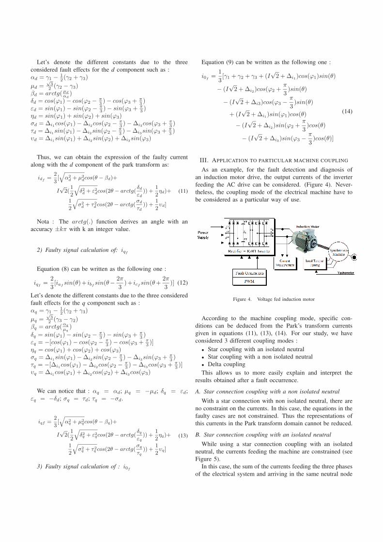
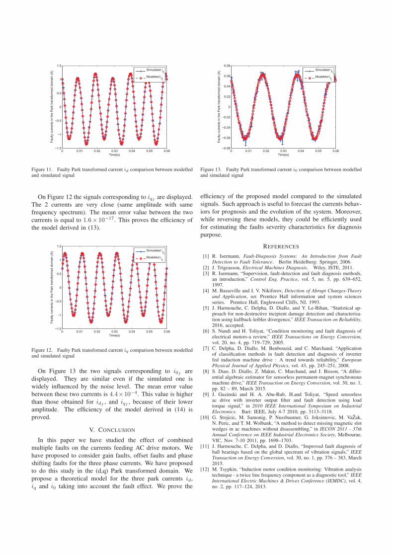
On Figure 12 the signals corresponding to iqf are displayed.The 2 currents are very close (same amplitude with samefrequency spectrum). The mean error value between the twocurrents is equal to 1.6× 10−17. This proves the efficiency ofthe model derived in (13).

0 0.01 0.02 0.03 0.04 0.05 0.06−1.5

−1

−0.5

0

0.5

1

1.5

Time(s)

Faulty c

urr

ents

in t

he P

ark

tra

nsfo

rmed d

om

ain

(A

) Simulated iq

f

Modelled iq

f

Figure 12. Faulty Park transformed current iq comparison between modelledand simulated signal

On Figure 13 the two signals corresponding to i0f aredisplayed. They are similar even if the simulated one iswidely influenced by the noise level. The mean error valuebetween these two currents is 4.4×10−4. This value is higherthan those obtained for idf

, and iqf , because of their loweramplitude. The efficiency of the model derived in (14) isproved.

V. CONCLUSION

In this paper we have studied the effect of combinedmultiple faults on the currents feeding AC drive motors. Wehave proposed to consider gain faults, offset faults and phaseshifting faults for the three phase currents. We have proposedto do this study in the (d,q) Park transformed domain. Wepropose a theoretical model for the three park currents id,iq and i0 taking into account the fault effect. We prove the

0 0.01 0.02 0.03 0.04 0.05 0.06−0.08

−0.06

−0.04

−0.02

0

0.02

0.04

0.06

0.08

Time(s)

Faulty c

urr

ents

in t

he P

ark

tra

nsfo

rmed d

om

ain

(A

) Simulated i0

f

Modelled i0

f

Figure 13. Faulty Park transformed current i0 comparison between modelledand simulated signal

efficiency of the proposed model compared to the simulatedsignals. Such approach is useful to forecast the currents behav-iors for prognosis and the evolution of the system. Moreover,while reversing these models, they could be efficiently usedfor estimating the faults severity characteristics for diagnosispurpose.

REFERENCES

[1] R. Isermann, Fault-Diagnosis Systems: An Introduction from Fault

Detection to Fault Tolerance. Berlin Heidelberg: Springer, 2006.[2] J. Trigeassou, Electrical Machines Diagnosis. Wiley, ISTE, 2011.[3] R. Isermann, “Supervision, fault-detection and fault diagnosis methods,

an introduction,” Control Eng. Practice, vol. 5, no. 5, pp. 639–652,1997.

[4] M. Basseville and I. V. Nikiforov, Detection of Abrupt Changes-Theory

and Application, ser. Prentice Hall information and system sciencesseries. Prentice Hall, Englewood Cliffs, NJ, 1993.

[5] J. Harmouche, C. Delpha, D. Diallo, and Y. Le-Bihan, “Statistical ap-proach for non-destructive incipient damage detection and characterisa-tion using kullback-leibler divergence,” IEEE Transaction on Reliability,2016, accepted.

[6] S. Nandi and H. Toliyat, “Condition monitoring and fault diagnosis ofelectrical motors-a review,” IEEE Transactions on Energy Conversion,vol. 20, no. 4, pp. 719–729, 2005.

[7] C. Delpha, D. Diallo, M. Benbouzid, and C. Marchand, “Applicationof classification methods in fault detection and diagnosis of inverterfed induction machine drive : A trend towards reliability,” European

Physical Journal of Applied Physics, vol. 43, pp. 245–251, 2008.[8] S. Diao, D. Diallo, Z. Makni, C. Marchand, and J. Bisson, “A differ-

ential algebraic estimator for sensorless permanent-magnet synchronousmachine drive,” IEEE Transaction on Energy Conversion, vol. 30, no. 1,pp. 82 – 89, March 2015.

[9] J. Guzinski and H. A. Abu-Rub, H.and Toliyat, “Speed sensorlessac drive with inverter output filter and fault detection using loadtorque signal,” in 2010 IEEE International Symposium on Industrial

Electronics. Bari: IEEE, July 4-7 2010, pp. 3113–3118.[10] G. Stojicic, M. Samonig, P. Nussbaumer, G. Joksimovic, M. VaŽak,

N. Peric, and T. M. Wolbank, “A method to detect missing magnetic slotwedges in ac machines without disassembling,” in IECON 2011 - 37th

Annual Conference on IEEE Industrial Electronics Society, Melbourne,VIC, Nov. 7-10 2011, pp. 1698–1703.

[11] J. Harmouche, C. Delpha, and D. Diallo, “Improved fault diagnosis ofball bearings based on the global spectrum of vibration signals,” IEEE

Transaction on Energy Conversion, vol. 30, no. 1, pp. 376 – 383, March2015.

[12] M. Tsypkin, “Induction motor condition monitoring: Vibration analysistechnique - a twice line frequency component as a diagnostic tool,” IEEE

International Electric Machines & Drives Conference (IEMDC), vol. 4,no. 2, pp. 117–124, 2013.