ANALYTICAL METHOD DEVELOPMENT

A MATHEMATICAL APPROACH

Katherin M. Schlipp

A Thesis Submitted to the University of North Carolina at Wilmington in Partial Fulfillment

Of the Requirements for the Degree of Master of Science

Department of Chemistry

University of North Carolina at Wilmington

2004

Approved by

Advisory Committee

Chair Accepted by

Dean, Graduate School

ii

TABLE OF CONTENTS

ABSTRACT....................................................................................................................... iv

ACKNOWLEDGMENTS .................................................................................................. v

DEDICATION................................................................................................................... vi

LIST OF TABLES............................................................................................................ vii

LIST OF FIGURES ......................................................................................................... viii

INTRODUCTION .............................................................................................................. 1

Method Development Theory of a Binary System ......................................................... 5

Column Hold-Up Volume and Column Hold-Up Time ................................................. 6

Method Development of a Binary System...................................................................... 7

Isoelutropic Binary Expression....................................................................................... 8

Applying Mixtures of Organic Solvents......................................................................... 9

Simplex Approach ........................................................................................................ 10

Mixture Design Approach ............................................................................................ 11

Optimization by Factorial Design................................................................................. 13

EXPERIMENTAL............................................................................................................ 13

Equipment ..................................................................................................................... 13

Determination of the Column Hold-Up Time............................................................... 15

Determination of the Gradient Delay Time .................................................................. 15

Computer Software and Program ................................................................................. 15

Chemical Information ................................................................................................... 18

Procedure ...................................................................................................................... 18

RESULTS AND DISCUSSION....................................................................................... 20

Effect of pH .................................................................................................................. 20

Method Development of a Binary System.................................................................... 28

iii

Optimization of pH ....................................................................................................... 35

Isoelutropic Binary Method Development ................................................................... 38

Applying Mixtures of Organic Solvents....................................................................... 46

Column Temperature Optimization .............................................................................. 53

Dissolution Method Development ................................................................................ 68

CONCLUSION................................................................................................................. 72

REFERENCES ................................................................................................................. 75

APPENDIX .......................................................................................................................77

iv

ABSTRACT Drug development relies strongly on the construction of optimal analytical

methods in an abbreviated timeframe in order to identify a final formulation and get to

market quickly. Simplification of the analytical development process for multiple active

products potentially provides a company with higher revenue as well as general cost

reductions. This research strongly demonstrates the benefits of using systematic and

mathematical approaches when developing analytical methods for a complex mixture.

By performing two gradient runs having different gradient slopes, and using a

mathematical relationship between retention times of each solute for each gradient and

each solute’s characteristic values, sj and k’j,w, the optimum gradient method for the

separation of diclofenac, propoxyphene, and their respective impurities was developed.

The method was further optimized by adjustment of the pH.

Using a mixture design approach, an isocratic method for a ternary system was

developed for the aforementioned separation, which required three experiments to find

the optimum mobile phase composition. A binary system for an isocratic separation was

also developed. Development of this method was optimized by investigating the

variations of characteristic values of each solute as a function of column temperature.

Additionally, a dissolution method was designed to mimic the release of

diclofenac and propoxyphene once the drug product is ingested into the human body. A

rapid isocratic HPLC method was developed for the determination of the amount of

diclofenac and propoxyphene that is dissolved in dissolution samples.

v

ACKNOWLEDGMENTS

I would like to give sincere thanks to Dr. Dean Shirazi for his help, guidance,

enthusiasm and encouragement. His strong knowledge of mathematics and

chromatography was a tremendous asset throughout the course of this research and I am

privileged and honored to have worked with him. I am grateful for Dr. Tania Toney-

Parker who brain-stormed the idea of this particular combination product. She has

thoughtfully given encouragement and support. I would also like to express my

gratitude to Dr. John Tyrell, who has graciously given guidance throughout the Master’s

program. I would like to thank Dr. Ned Martin whose opinions I value and respect. I

would like to acknowledge Chuck Bon and Lisa Olsen who processed results in SAS so

quickly. Your help was invaluable and contributed to the success of my research. I

would like to thank Mrs. Sherry Layton who always knew exactly what I was going

through each day. Her encouragement and support has meant so much and I have found

a friend for life. I am forever grateful to my husband, Michael, who sacrificed our time

so that I could succeed. Special thanks go to my parents, William and Debbie, who gave

endless loving support. Finally, I would like to acknowledge aaiPharma for the support

both financially and professionally. I cannot express how grateful I am for this fantastic

opportunity.

vi

DEDICATION

I would like to dedicate this thesis to my husband, Michael, who has always

believed in me.

vii

LIST OF TABLES

Table Page 1. Calculated characteristic values of s and k’j,w at pH 2.5 using SAS, based on Schoenmakers’ equations ....................................................22 2. Calculated characteristic values of s and k’j,w at pH 6.8 using SAS, based on Schoenmakers’ equations ....................................................24 3. Calculated characteristic values of s and k’j,w at pH 9.0 using SAS, based on Schoenmakers’ equations ....................................................26 4. Calculated characteristic values of s and k’j,w at pH 2.5 using SAS, based on Schoenmakers’ equations ....................................................29 5. Predicted retention times versus actual retention times for isocratic separation using a mobile phase buffer, pH 2.5 and acetonitrile in a volumetric ratio of 60:40.......................................................34 6. Calculated characteristic values of s and k’j,w at pH 2.5 using SAS, based on Schoenmakers’ equations ....................................................42 7. Resolution measurements for binary systems with acetonitrile and methanol and ternary system of acetonitrile and methanol.............................55 8. Retention time measurements for binary systems with acetonitrile and methanol and ternary system of acetonitrile and methanol.............................56 9. Predicted retention times versus actual retention times for isocratic separation using a 5 µm particle size column a mobile phase buffer, pH 3.5 and acetonitrile in a volumetric ratio of 66:34 ...............................58 10. Calculated ∆H in equilibrium between the mobile phase and stationary phase......................................................................................................62 11. Calculated characteristic values of s and k’j,w at pH 3.5 and column temperature of 60°C using SAS, based on Schoenmakers’ equations ................................................................................................................64 12. Predicted retention times vs. actual retention times for isocratic separation using a 5 µm particle size column at 60°C, a mobile phase of buffer, pH 3.5 and acetonitrile in a volumetric ratio of 65:35...........................67 13. Dissolution results of a research prototype............................................................71

viii

LIST OF FIGURES Figure Page 1. Overlapping mixture design model........................................................................12 2. Factorial design......................................................................................................14 3. Chromatogram of sodium nitrate for the measurement of void time of the column .................................................................................................16 4. Chromatogram of a breakthrough curve using acetone to calculate the delay time of the gradient.................................................................................17 5. Plot of ln k’ vs. organic fraction at pH 2.5 based on Schoenmakers’ equations.......................................................................................23 6. Plot of ln k’ vs. organic fraction at pH 6.8 based on Schoenmakers’ equations.......................................................................................25 7. Plot of ln k’ vs. organic fraction at pH 9.0 based on Schoenmakers’ equations.......................................................................................27 8. Plot of ln k’ vs. organic fraction at pH 2.5 based on Schoenmakers’ equations.......................................................................................30 9 Chromatogram of a mixture solution, 1.2% per minute gradient slope using acetonitrile as organic modifier ............................................32 10. Chromatogram of mixture solution for isocratic method using 40:60, acetonitrile:phosphate buffer, pH 2.5, as the mobile phase ...................................33 11. Chromatogram of mixture solution, 1.2% per minute gradient slope, acetonitrile as organic modifier in mobile phase, pH 2.5 ......................................36 12. A plot of ln k’ vs. pH when the percentage of organic in the mobile phase is held at 35%...................................................................................37 13. Chromatogram of mixture solution, 1.2% per minute gradient slope, acetonitrile as organic modifier, pH 3.5 ......................................................39 14. A plot of ln k’ vs. organic fraction, pH 3.5, 5 µm particle size column....................................................................................................................43 15. Chromatogram of a mixture solution from an isocratic run using 34% acetonitrile, pH 3.5...............................................................................44

ix

16. Chromatogram of a mixture solution, isocratic method using 44% methanol in the mobile phase, pH 3.5 ...........................................................45 17. Chromatogram overlay of mixture solution for isocratic runs using 34% acetonitrile and 44% methanol.............................................................47 18. Chromatogram of a mixture solution, 47% methanol............................................48 19. Chromatogram overlay of mixture solution at 34% acetonitrile and 47% methanol..................................................................................................49 20. Mixture design model for ternary mobile phase ....................................................50 21. Chromatogram of mixture solution in ternary system (12:26:62,

methanol:acetonitrile:phosphate buffer, pH 3.5) ...................................................52 22. Chromatogram of mixture solution for optimal isocratic ternary system ........................................................................................................54 23. Chromatogram of mixture solution from an isocratic run having a mobile phase of 34:66 acetonitrile:buffer, pH 3.5 at various column temperatures from 0-5 minutes ..............................................................................59 24. Chromatogram of mixture solution from an isocratic run having a mobile phase of 34:66 acetonitrile:buffer, pH 3.5 at various column temperatures from 0-85 minutes ............................................................................60 25. Plot of ln k’ vs. the inverse of the temperature where the ∆H = -slope × R .....................................................................................................61 26. A plot of ln k’ vs. organic fraction, pH 3.5, 5 µm particle size column at 60°C ......................................................................................................65 27. Chromatogram of mixture solution with 5 µm particle size column at 60°C with mobile phase of buffer, pH 3.5:acetonitrile 65:35............................66 28. Chromatogram overlay of a standard and sample solution using a mobile phase of 45:55, acetonitrile:phosphate buffer, pH 3.5 ............................70

INTRODUCTION

As part of the formulation development of new pharmaceutical product lines, it is

necessary to develop, optimize and validate reliable and meaningful analytical methods to

support the integrity of a new product. Analytical methods are utilized for the

characterization of the active pharmaceutical ingredient and its degradation profile, as

well as a tool for the assessment, selection and optimization of prototypes. Analytical

methodology is mandated by the FDA for determining the efficacy and safety of the final

product and as a means of establishing a commercial shelf life. Analytical methods are

the foundation for the success of any drug development (Green, 1996).

The safety and efficacy of a drug product is related to the purity of the drug and

the formation of impurities that may potentially induce toxicological side effects.

Therefore, efforts are made in the pharmaceutical industry to minimize impurities in

active pharmaceutical ingredients and to control the degradation pathways of final

formulations. Specific analytical methods are used to monitor the potency, process

impurities, and any degradation impurities of both the drug substance and drug product

during stability to assure the drug’s safety and therapeutic activity.

High performance liquid chromatography (HPLC) is the preferred method for the

quantitation of actives and impurities in pharmaceutical products because of its

sensitivity, accuracy, specificity, separation capacity and widespread applicability

(Snyder, 1997). Thus, development of a single reliable method for these actives and their

impurities is necessary to save time and costs during prototype development, release of

the new product, and lengthy stability studies.

2

Not only are analytical methods used to characterize the drug substance and drug

product on the shelf but they may also serve as predictive tools to establish in-vivo

response. For example, discriminating dissolution tests are developed to simulate the in-

vivo environment. Based upon the defined marketed product label, a release profile may

be adjusted using the dissolution rate. An optimal dissolution method not only can be

used for prototype selection, it can also demonstrate batch to batch uniformity to assure

product performance and can also be used to assess bioavailability which may replace the

need for multiple bioequivalence clinical studies (Crison). It is also necessary to

establish an in-vitro to in-vivo correlation where the dissolution will simulate the drug

disintegration, dissolution, and solubilization in the aqueous environment of the

gastrointestinal (GI) tract. Appropriate dissolution methods are also used for quality

control purposes; product dissolution needs to be consistent with a minimal relative

standard deviation. Dissolution testing serves a variety of purposes and can be a

meaningful tool for assessing potential changes in bioavailability over the duration of

stability.

It is very common for analysts in industry to begin HPLC method development

using a non-systematic and non-mathematical approach when developing an analytical

method. For example, an analyst will usually initiate development of an isocratic run

with a certain percentage of organic solvent based on the analyst’s previous experience or

based on a literature method for a similar analyte and then make stepwise adjustments.

The retention time of an analyte in reversed phase chromatography decreases when the

percentage of organic is increased. Thus, the desired composition of mobile phase can be

estimated using this technique. However, this approach is based on trial-and-error and

3

does not necessarily produce optimum separation especially for a multiple component

system, which has several actives, related substances and impurities. The trial-and-error

approach, although simple and easy to apply, suffers from serious drawbacks as it is

laborious and contains many uncertainties.

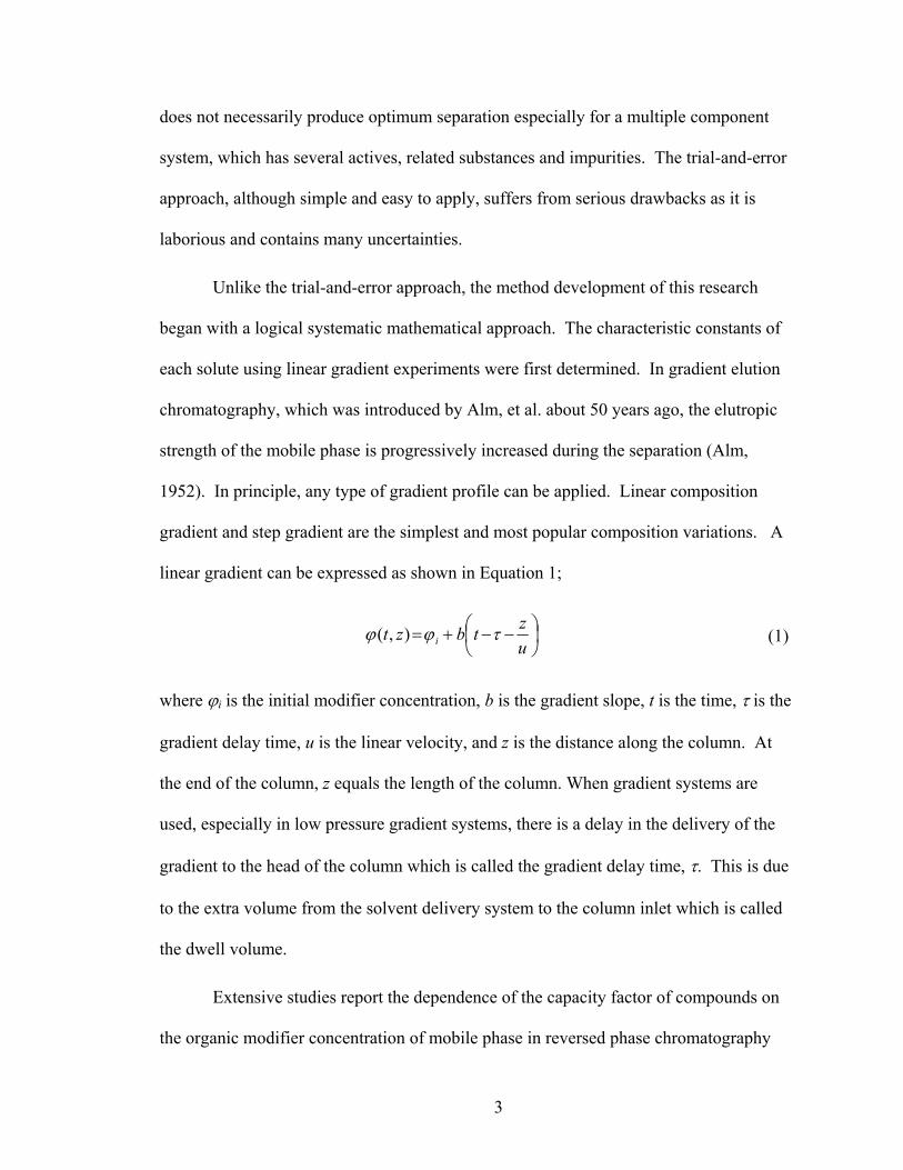
Unlike the trial-and-error approach, the method development of this research

began with a logical systematic mathematical approach. The characteristic constants of

each solute using linear gradient experiments were first determined. In gradient elution

chromatography, which was introduced by Alm, et al. about 50 years ago, the elutropic

strength of the mobile phase is progressively increased during the separation (Alm,

1952). In principle, any type of gradient profile can be applied. Linear composition

gradient and step gradient are the simplest and most popular composition variations. A

linear gradient can be expressed as shown in Equation 1;

⎟⎠⎞

⎜⎝⎛ −−+=

uztbzt i τϕϕ ),( (1)

where ϕi is the initial modifier concentration, b is the gradient slope, t is the time, τ is the

gradient delay time, u is the linear velocity, and z is the distance along the column. At

the end of the column, z equals the length of the column. When gradient systems are

used, especially in low pressure gradient systems, there is a delay in the delivery of the

gradient to the head of the column which is called the gradient delay time, τ. This is due

to the extra volume from the solvent delivery system to the column inlet which is called

the dwell volume.

Extensive studies report the dependence of the capacity factor of compounds on

the organic modifier concentration of mobile phase in reversed phase chromatography

4

Synder, 1980; Jandera, 1985). These studies indicate that, within a reasonable range, the

dependence can be expressed as shown in Equation 2 which can be written as Equation 3;

ϕϕ jswjj ekk ,')(' = (2)

ϕϕ jwjj skk += ,'ln)('ln (3)

where sj is the slope of the logarithmic plot, and k’j,w = k’j (ϕ = 0) is the capacity factor of

the solute in pure weak eluent (such as water or buffer). k’j,w and sj are the characteristic

constants of each solute. In a wider range of modifier concentration, a quadratic

relationship may give a better account for the dependence of ln k’j (Equation 4).

2,'ln)('ln ϕϕϕ bakk wjj +−= (4)

In order to predict the retention time of each solute (j) at any specific composition

of organic modifier (ϕ), the value of ln k’j,w and sj should be determined. There are two

procedures for their determination. The first involves injection of a solution of each

solute at various isocratic conditions (various ϕ) and determining k’j from the retention

times using Equation 5 then plotting ln k’j versus ϕ for each solute. This procedure is

cumbersome and time consuming.

0

0'

ttt

k jrj

−= (5)

A simpler and more accurate procedure is to run two linear gradients of a mixture

of solutes with different slopes and record the retention time of each solute in each

gradient run.

5

Method Development Theory of a Binary System

It has been shown that the retention time of each solute in a linear gradient,

provided that the solute elutes before the completion of the gradient, is given by Equation

6 (Snyder, 1980; Schoenmakers, 1978 and 1991).

001ln1 tτkkτtbs

bst

i

i

j jj

jj

r ++⎪⎭

⎪⎬⎫

⎪⎩

⎪⎨⎧

⎥⎥⎦

⎤

⎢⎢⎣

⎡′×

⎟⎟

⎠

⎞

⎜⎜

⎝

⎛

′−×−×

×−=

ϕ

ϕ

(6)

where trj, is the retention time of a solute (j) in each gradient run, sj is the slope of the

graph of ln kj’ vs. ϕ, b is the gradient slope, t0 is the column hold-up time, τ is the

gradient delay time, and k’jφ i, is the capacity factor of a solute (j) at the start of the

gradient (φ = φi). In many cases, k’jφ i is very large so that t0 >> τ / k’jφ i and sj b k’jφ i t0

>>1. Therefore, Equation 6 can be simplified to Equation 7.

( ) 00 'ln1 tkbtsbs

tijj

jrj ++×

×−= τ

ϕ (7)

Equation 6 is valid only for solutes that elute before the completion of the

gradient (ϕ = ϕf) (Schoenmakers, 1978). For solutes that elute after the completion of the

gradient, Schoenmakers defines the following analytical solution (Equation 8 and 9) to

predict the retention times in the gradient run (Schoenmakers, 1978).

(8)

(9) ( ) ( ) ( )ijj 'ln'ln ϕϕϕϕ −+= fjif skk

( ) 0ijjj

j0j ''

''

' tb

kkbs

kk

tkt fif

j

f

ifrj

++−

−−×

+⎟⎟⎠

⎞⎜⎜⎝

⎛−= τ

ϕϕτϕϕ

ϕ

ϕϕ

6

Where k’jφ i is the capacity factor at the beginning of the gradient and k’jφ f is the capacity

actor at the end of the gradient. Equation 8 was investigated when the predicted retention

time results obtained using this equation were very different than actual measured

retention times. By re-deriving this equation as shown in Appendix A, a mathematical

error was found in Equation 8 and the following equation was derived (Equation 10);

(10)

where k’jφ f is related to k’jφ i through Equation 9.

Column Hold-Up Volume and Column Hold-Up Time

In order to use Equation 6 or 10, the value of the column hold-up time must be

determined. The volume of the mobile phase required to elute a non-retained component

is called the column hold-up volume and the corresponding time is called the column

hold-up time. They are related according to Equation 11;

(11)

where V0 and t0 are column hold-up volume (mL) and column hold-up time (minutes) and

Fv is the mobile phase flow rate (mL per minute). The column hold-up volume, V0, and

hold-up time, t0, are characteristics of a column. Different methods for the determination

of the hold-up time have been reviewed in detail (Grushka, 1982). It is usually measured

by injecting an inert or non-retained tracer. Unlike gas chromatography, the definition

and determination of the hold-up volume is not straight forward. The density of the

mobile phase in the bulk mobile phase and that in the monolayer in contact with the

surface of the stationary phase is not usually the same. The situation is more complex in

0j

jj

j0j '

''1'

' tbk

kkbsk

tkt fi

i

if

jifrj

++−

−⎟⎟⎠

⎞⎜⎜⎝

⎛ −

×+⎟

⎟⎠

⎞⎜⎜⎝

⎛−= τ

ϕϕτ

ϕ

ϕϕ

ϕϕ

00 tFV v ×=

7

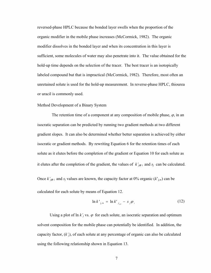
reversed-phase HPLC because the bonded layer swells when the proportion of the

organic modifier in the mobile phase increases (McCormick, 1982). The organic

modifier dissolves in the bonded layer and when its concentration in this layer is

sufficient, some molecules of water may also penetrate into it. The value obtained for the

hold-up time depends on the selection of the tracer. The best tracer is an isotopically

labeled compound but that is impractical (McCormick, 1982). Therefore, most often an

unretained solute is used for the hold-up measurement. In reverse-phase HPLC, thiourea

or uracil is commonly used.

Method Development of a Binary System

The retention time of a component at any composition of mobile phase, ϕ, in an

isocratic separation can be predicted by running two gradient methods at two different

gradient slopes. It can also be determined whether better separation is achieved by either

isocratic or gradient methods. By rewriting Equation 6 for the retention times of each

solute as it elutes before the completion of the gradient or Equation 10 for each solute as

it elutes after the completion of the gradient, the values of k’jφ i and sj can be calculated.

Once k’jφ i and sj values are known, the capacity factor at 0% organic (k’j,w) can be

calculated for each solute by means of Equation 12.

(12)

Using a plot of ln k’j vs. ϕ for each solute, an isocratic separation and optimum

solvent composition for the mobile phase can potentially be identified. In addition, the

capacity factor, (k’j), of each solute at any percentage of organic can also be calculated

using the following relationship shown in Equation 13.

iln'ln wj, ϕϕ jj sk'k

i−=

8

(13)

The retention time can then be calculated from the k’j,φ for any given ϕ with Equation

14.  

 (14)

Isoelutropic Binary Expression

When the optimum separation with a certain organic modifier (such as

acetonitrile) is determined using the aforementioned approach and still the separation of

all peaks of interest is not achieved, the next step in method development is to change the

organic modifier to a different solvent. The concentration of the new organic modifier

(such as methanol or tetrahydrofuran) in the new binary system, which is predicted to

yield a chromatogram exhibiting the same range of k’ values, can be calculated using the

“transfer rule” equation (Schoenmakers, 1981).

After selecting the acetonitrile-buffer elutropic strength, ϕACN, using the

aforementioned approach, which produces an optimum chromatogram in which all

solutes of the mixture elute with a suitable range of retention times, calculation of

equivalent elutropic strength relative to ϕACN, for methanol-buffer and THF-buffer can be

performed using the solvent polarity scale first described by Snyder in 1974. All binary

eluents with equivalent solvent polarity are, to a first approximation, assumed to be

isoelutropic. The expression given by Snyder for calculating the solvent polarity is

shown in Equation 15;

BBAAmixture PPP ''' ϕϕ += (15)

ϕϕ jwj sk'k += ,j, ln 'ln

) '(1 j,0 ϕkttjr +×=

9

where φ A and φ B are the volume fraction of solvents A and B and P’A and P’B are the

polarity index values of the pure solvents A and B. The P’ value for water, methanol,

acetonitrile, and tetrahydrofuran (THF) are 9.0, 6.6, 6.2, and 4.2 respectively. An

alternative approach for obtaining the composition of isoelutropic binary solvents is

derived by Schoenmakers (1981). Based on the isocratic retention behavior of a set of 32

solutes in all three binary eluents (acetonitrile-water, methanol-water, and THF-water),

“transfer rule” equations relating isoelutropic volume fractions were expressed in

Equations 16 and 17.

MeOHMeOHACN ϕϕϕ 57.032.0 2 += (16)

MeOHTHF ϕϕ 66.0= (17)

Equations 16 and 17 represent an average of the eluent transfer behaviors of each

of the solutes of the data set considered. The scatter of these average predicted values is

fairly large such that a large deviation between predicted and actual isoelutropic volume

fractions is observed in practice. Therefore, these equations provide only a first approx-

imation prediction of equivalent elutropic strengths among the three binary eluents. A re-

evaluation of these “transfer rule” equations are described by Herman, et al. who

proposed Equations 18 and 19 for isoelutropic volume correlation (Herman,1989).

MeOHMeOHMeOHACN ϕϕϕϕ 447.0953.049.0 23 ++−= (18)

MeOHMeOHMeOHTHF ϕϕϕϕ 423.0702.042.0 23 ++−= (19)

Applying Mixtures of Organic Solvents

When an isocratic separation is not successful using any of the binary systems, it

may be necessary to use a ternary or quaternary system. In recent years, many practical

10

examples of the advantages to use of ternary mobile phase in reversed phase liquid

chromatography have been published (Bakalyar, 1977; Glajch, 1980). Bakalyar, et al.

(1977) performed the first systematic investigation of a ternary mobile phase. Glajch, et

al. (1980) studied the behavior of ternary and quaternary mixtures of water, acetonitrile,

methanol, and THF. They also describe a procedure for an optimization of a multi-

component mobile phase. Schoenmakers, et al (1981). reported a systematic study of the

retention behavior of two ternary mobile phase systems (methanol, acetonitrile, water and

methanol, THF, water). They showed that the relationship of the logarithm of the

capacity factor to the volume fraction of the two organic modifiers can be expressed by a

quadratic equation (Schoenmakers, 1981).

constant'ln 2112211222

211 +++++= ϕϕϕϕϕϕ DBBAAk (20)

There are a number of alternative methods in the literature for optimizing ternary

and quaternary separations and these include the simplex approach and the mixture

design approach.

Simplex Approach

One approach for optimizing ternary and quaternary separations is the sequential

simplex method which was first proposed by Spendly, et al. in 1962 (Berridge, 1988).

The simplex procedure is a hill-climbing method in which the direction of advance is

dependent solely on the ranking of responses (Berridge, 1988). The great advantage of

the simplex procedure in the optimization of liquid chromatography separations is that it

is able to optimize many inter-dependent variables without prior knowledge about the

mode of separation or the complexity of the samples. It also does not require any pre-

11

conceived model for the retention behavior of solutes. There are however, significant

disadvantages associated with simplex optimization. Most notable is the problem of

locating a local rather than a global optimum. An additional disadvantage is the large

number of experiments required.

Mixture Design Approach

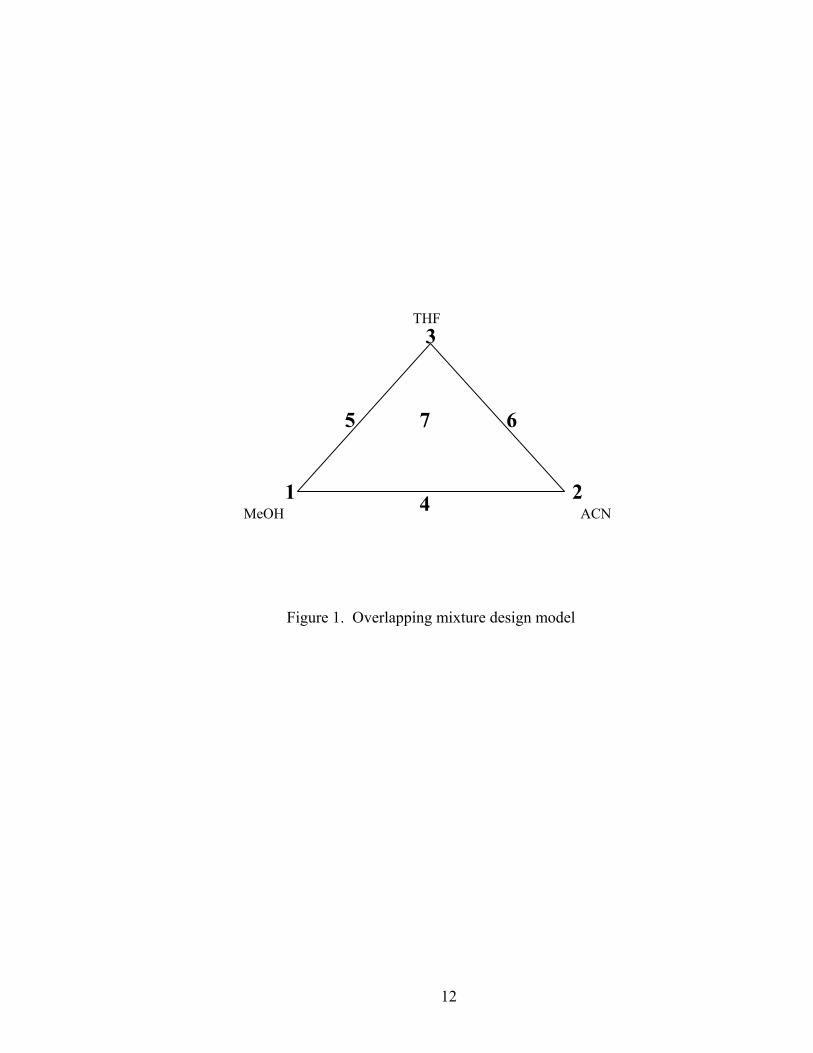
Another approach for optimizing ternary and quaternary separations is the mixture

design approach. This statistical approach is suitable for related variables. Related

variables are those that directly affect each other. For example, the sum of the mobile

phase composition must be 100% at all times, so individual mobile phase solvents are

related variables. This approach is well known in statistical literature (Cornell, 1981).

The mixture design statistical approach for mobile phase optimization is illustrated in

Figure 1. Seven experiments are employed to fit experimental retention data (ln k’) to a

second order polynomial equation with respect to three mobile phase modifiers. In the

case of reversed-phase liquid chromatography, the mobile phase carrier, water or buffer,

is modified with acetonitrile, methanol, and tetrahydrofuran (THF). In normal phase, n-

hexane or n-heptane is the carrier solvent and it is modified with chloroform, methylene

chloride, and methyl-tertbutyl ether (MTBE). Retention (k’) values are measured for

each component in the mixture using the seven mobile phase solvent mixtures shown in

Figure 1. These data are then fitted to a second order polynomial to obtain the constants

in the following equations, from which the optimum mobile phase composition can be

determined (Glajch, 1983).

(21)

For a Quaternary System:

3213,2,1313,1323,2212,1332211

'ln xxxaxxaxxaxxaxaxaxak j ++++++=

12

Figure 1. Overlapping mixture design model

MeOH ACN

THF

X X 1 4 2

7

3

5 6

13

(22)

This systematic approach can determine the optimum ratio of mobile phase with a

small number of experiments. Instead of ln k’, the resolution of each peak pair in the

system also can be mapped using the same methodology (Glajch, 1983; Ong, 1995).

Optimization by Factorial Design

Unlike mobile phase composition, pH and temperature are discrete variables since

they have little direct effects on each other or on other mobile phase or stationary phase

components. For discrete variables such as temperature and pH, the factorial design is

suitable. Figure 2 illustrates a factorial design for optimization of temperature (20-40 °C)

and pH (3-5) effects in liquid chromatography that employs nine experiments (3 levels

and two factors) to fit the retention time data (ln k’) of each solute in these nine

experiments to a second order polynomial to determine the optimum temperature and pH

(Glajch, 1983).

EXPERIMENTAL Equipment

The high performance liquid chromatography (HPLC) equipment used for all

experiments was a Hewlett-Packard 1100 equipped with a gradient pump, autosampler,

temperature controlled column compartment and an ultraviolet wavelength detector. The

columns used in the experiments were X-Terra MS C18, 150 × 4.6 mm, 3.5 µm particle

size and X-Terra RP C18, 150 × 4.6 mm, 5.0 µm particle size. The X-terra columns were

selected because of their ability to withstand higher pHs. Potassium phosphate

For a Ternary System:

212,12211'ln xxaxaxak j ++=

14

Figure 2. Factorial design

1 2

34

6

5

9

7

8pH

Temperature

5 4 3

20C 30C 40C

15

monobasic at a concentration of 50 mM was used for the aqueous portion of the mobile

phases in combination with organic solvents acetonitrile, methanol or both. Injections

were analyzed at 217 nm. The low wavelength enhanced the detection of most solutes.

Determination of the Column Hold-Up Time A measurement of the column hold-up time, t0, was needed in the calculations to

predict the retention times. It was measured by an injection of a sodium nitrate solution,

an inert compound at a low concentration. A small peak eluted within the solvent front

(Figure 3). The retention time of this peak is equal to the column hold-up time.

Determination of the Gradient Delay Time

A measurement of the gradient delay time, τ, is necessary to predict the retention

time of the solutes. To measure the delay time, τ, a step gradient was used. To perform

frontal analysis, the mobile phase must contain a chromophore such as acetone to

promote UV absorption. A solution of 1% acetone in methanol was prepared and used as

solvent B. Pure methanol was used as solvent A. The column was disconnected and the

inlet and outlet tubing were connected using a dead volume union. The HPLC system

was equilibrated with solvent A (100% methanol). After 2 minutes of Solvent A, the

mobile phase was switched to solvent B (1% acetone in methanol) giving a breakthrough

curve as shown in Figure 4. The gradient delay time is measured using the breakthrough

curve.

Computer Software and Program

Waters Millennium 4.0 was used as the data acquisition program to collect

chromatograms for each injection and to measure the retention times and resolutions. For

16

T; Date Acquired: 5/14/2003 4:11:16 PM; Channel Id 3242

50.00

55.00

60.00

65.00

70.00

75.00

80.00

85.00

90.00

95.00

100.00

105.00

110.00

115.00

120.00

Minutes0.00 1.00 2.00 3.00 4.00 5.00 6.00 7.00 8.00 9.00 10.00

Figure 3. Chromatogram of sodium nitrate for the measurement of void time of the column

17

T; Date Acquired: 3/17/2003 3:43:46 PM; Channel Id 1783

mV

40.00

60.00

80.00

100.00

120.00

140.00

160.00

180.00

200.00

220.00

240.00

Minutes0.00 1.00 2.00 3.00 4.00 5.00 6.00 7.00 8.00 9.00 10.00

Figure 4. Chromatogram of a breakthrough curve using acetone to calculate the delay time of the gradient

X

18

the calculations of k’jφ i and s from equation 6 and/or 10 using data input (retention times

of solutes, trj, gradient delay time, τ, column hold-up time, t0 and gradient slope, b), a

non-linear modeling program in SAS® PC version 6.12 was used to solve for these

parameters. Microsoft Excel 2003 was used to calculate k’j,w and to create the plots of ln

k’j versus organic fraction. Excel was also used during isoelutropic and mixture design

experiments to calculate the optimum mobile phase composition.

Chemical Information

The following list provides the names of the actives and available related

substances that were used in this research. Individual solutions were prepared at a

concentration of 0.2 mg/mL for the actives and 0.002 mg/mL for the related substances

and process impurities.

List of Components Component Type Propoxyphene Napsylate Active Diclofenac Potassium/Diclofenac Sodium Active 2-Indolinone Related Substance Propoxyphene Related Compound A (Prop Rel Cmpd A) Related Substance Propoxyphene Related Compound B (Prop Rel Cmpd B) Related Substance Cis-4-dimethylamino-1,2-diphenyl-3-methyl-butene (CT1) Related Substance Diclofenac Related Compound A (Diclo Rel Cmpd A) Related Substance [2-[(2,6-Dichlorophenyl)amino]phenyl]methanol (Alcohol) Related Substance 2-Chloro-n-(2,6-dichlorophenyl)acetamide (2 Chloro) Process Impurity 2,6-Dichlorodiphenylamine (Dichloro) Process Impurity 2-[(2.6-Dichlorophenyl)amino]benzaldehyde (Aldehyde) Related Substance Procedure

Schoenmakers’ equations, Equations 23, 24, and 25, were implemented to predict

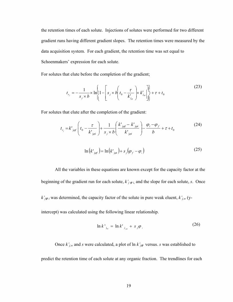
19

the retention times of each solute. Injections of solutes were performed for two different

gradient runs having different gradient slopes. The retention times were measured by the

data acquisition system. For each gradient, the retention time was set equal to

Schoenmakers’ expression for each solute.

For solutes that elute before the completion of the gradient;

001ln1 tkk

tbsbs

ti

i

j jj

jj

r ++⎪⎭

⎪⎬⎫

⎪⎩

⎪⎨⎧

⎥⎥⎦

⎤

⎢⎢⎣

⎡′×

⎟⎟

⎠

⎞

⎜⎜

⎝

⎛

′−×−×

×−= ττ

ϕ

ϕ

(23)

For solutes that elute after the completion of the gradient:

(24)

(25)

All the variables in these equations are known except for the capacity factor at the

beginning of the gradient run for each solute, k’j φ i, and the slope for each solute, s. Once

k’jφ i was determined, the capacity factor of the solute in pure weak eluent, k’j,w (y-

intercept) was calculated using the following linear relationship.

(26)

Once k’j,w and s were calculated, a plot of ln k’jφ versus. s was established to

predict the retention time of each solute at any organic fraction. The trendlines for each

iwln'ln j ϕ

ϕ jj sk'ki+=

( ) ( ) ( )ijj 'ln'ln ϕϕϕϕ −+= fjif skk

0j

jj

j0j '

''1'

' tbk

kkbsk

tkt fi

i

if

jifrj

++−

−⎟⎟⎠

⎞⎜⎜⎝

⎛ −

×+⎟

⎟⎠

⎞⎜⎜⎝

⎛−= τ

ϕϕτ

ϕ

ϕϕ

ϕϕ

20

solute indicated the expected separation of each solute. The closer the trendlines

appeared in the plot, the less separation was expected in the chromatography.

RESULTS AND DISCUSSION

Effect of pH

For basic solutes, generally the retention time increases with increasing pH as

long as the pH does not exceed the log of the ionization constant for a base, pKb.

Typically, basic solutes are protonated at a pH lower than their pKb. As pH increases,

the ionization of the base decreases, the solute becomes hydrophobic, preferring the non-

polar stationary phase which increases the retention time. However, the decrease in

retention time at a pH higher than pKb cannot be explained in this way. The degree of

protonation of the solute and the residual silanol group must also be considered. By

increasing the pH of the mobile phase, more residual silanol groups are negatively

charged and these groups behave as a weak cation exchanger. When the pH of the

mobile phase is higher than the pKb of the solute, the protonation of the basic solute is

suppressed causing less interaction with residual silanol groups and therefore decreasing

the retention time. The influence of pH on the retention of acidic solutes is the opposite

of that observed with basic solutes. The retention times of the acidic solutes decreases

with increasing pH. Acids are negatively charged at pH higher than the log of the

ionization constant for an acid, pKa, preferring the polar mobile phase. A second reason

for the decreased retention time might be that at higher pH the residual silanol groups and

the acidic solute are negatively charged so the solute is excluded from the stationary

phase. The decrease in retention time is more pronounced for stronger acids than for

weaker acids.

21

In order to determine the behavior of the solutes based on their sensitivity to pH

of the mobile phase, two gradient runs, each with different gradient slopes were

performed for pH 2.5, 6.8, and 9. The experiments employed the X-Terra MS 150 x 4.6

mm, 3.5 µm particle size column with a flow rate of 1.0 mL/minute. Mobile phase A was

buffer and acetonitrile in a volumetric ratio of 90:10 and mobile phase B was buffer and

acetonitrile in a volumetric ratio of 35:65. The first gradient slope was 1.6% per minute

or 2% to 98% mobile phase B in 37 minutes and the second gradient slope was 1.1% per

minute or 2% to 98% mobile phase B in 55 minutes. After the completion of the

gradient, the mobile phase remained at the final composition for at least 10 minutes to

allow any late eluting solutes to elute during the run time. The retention time of each

solute was measured for each gradient run at each pH. The slopes, s, and capacity factors

in pure weak solvent (kj,w) were calculated by SAS (Tables 1-3). Plots of ln k’j versus the

fraction of organic (φ ) were established for each pH (Figure 5-7).

Because most of the solutes are basic, the retention time increased as the pH

increased. Generally, a low pH of about 2.5 to 3.0 is a good starting point for the

separation of the mixture of acids and bases. At this pH range, the basic solutes are less

retained as they are protonated while the acidic solutes exhibit greater retention as they

are mainly non-ionic. Therefore, both acidic and basic solutes can be separated within a

reasonable analysis time. The results of this study confirmed the general rule that at

higher pH, generally, acidic solutes are less retained and basic solutes are more retained

resulting in a long impractical analysis time. As shown from the plots in Figures 5-7, the

run time is increased with increasing pH at a certain percentage of organic modifier. The

run time can be decreased by increasing the percent of organic in the mobile phase;

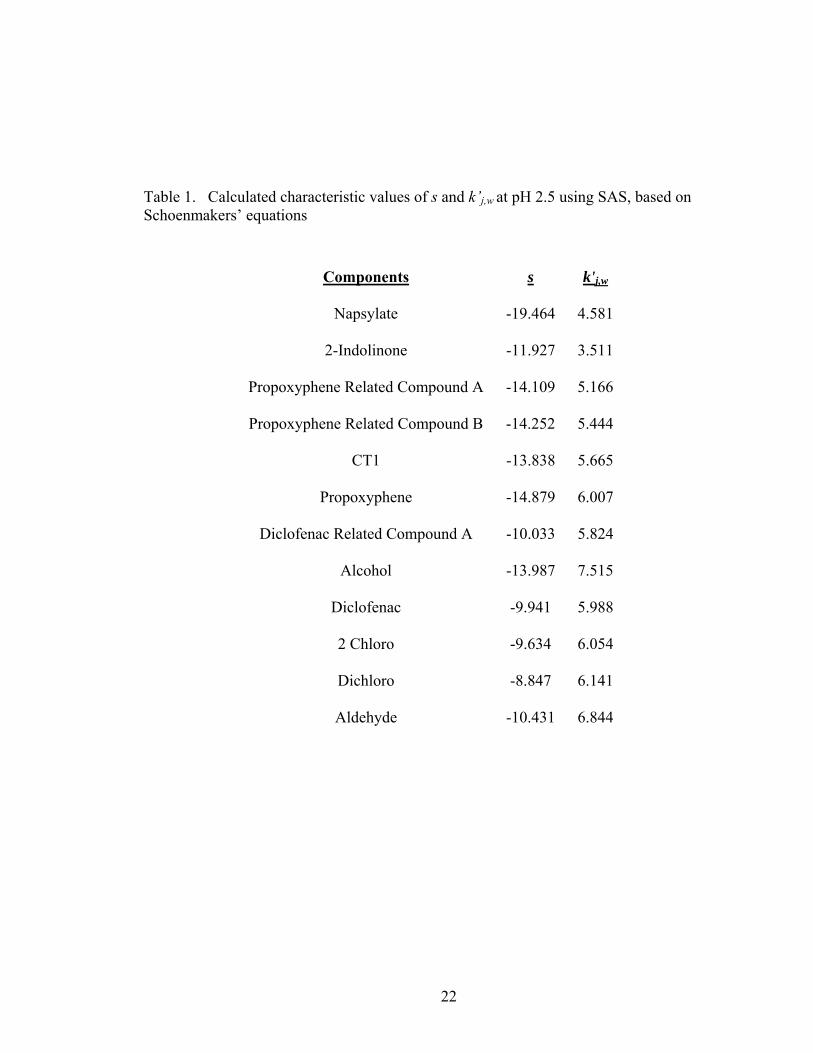
22

Table 1. Calculated characteristic values of s and k’j,w at pH 2.5 using SAS, based on Schoenmakers’ equations

Components s k'j,w

Napsylate -19.464 4.581

2-Indolinone -11.927 3.511

Propoxyphene Related Compound A -14.109 5.166

Propoxyphene Related Compound B -14.252 5.444

CT1 -13.838 5.665

Propoxyphene -14.879 6.007

Diclofenac Related Compound A -10.033 5.824

Alcohol -13.987 7.515

Diclofenac -9.941 5.988

2 Chloro -9.634 6.054

Dichloro -8.847 6.141

Aldehyde -10.431 6.844

23

ln k' vs. Organic Fraction

-3.0

-2.0

-1.0

0.0

1.0

2.0

3.0

4.0

5.0

6.0

0.1 0.15 0.2 0.25 0.3 0.35 0.4 0.45 0.5 0.55 0.6

Organic Fraction

ln k

'

Nap sylate 2 Ind o lino ne Pro p Rel Cmp d A Pro p Rel Cmp d B CT1 Pro p o xyp hene

Diclo Rel Cmp d A Alco ho l Diclo fenac 2 Chlo ro Dichlo ro Ald ehyd e

Figure 5. Plot of ln k’ vs. organic fraction at pH 2.5 based on Schoenmakers’ equations

24

Table 2. Calculated characteristic values of s and k’j,w at pH 6.8 using SAS, based on Schoenmakers’ equations

Components

s

k'j,w

Napsylate -16.230 4.152

2-Indolinone -13.321 3.563

Propoxyphene Related Compound A -10.688 5.357

Propoxyphene Related Compound B -12.283 5.936

CT1 -10.423 6.055

Propoxyphene -11.033 6.239

Diclofenac Related Compound A -10.918 6.716

Alcohol -11.012 7.057

Diclofenac -17.881 7.041

2 Chloro -10.612 7.097

Dichloro -10.505 7.574

Aldehyde -10.162 7.447

25

ln k' vs. Organic Fraction

-3.0

-2.0

-1.0

0.0

1.0

2.0

3.0

4.0

5.0

6.0

0.1 0.15 0.2 0.25 0.3 0.35 0.4 0.45 0.5 0.55 0.6

Organic Fraction

ln k

'

Napsylate 2 Indolinone Prop Rel Cmpd A Prop Rel Cmpd B CT1 PropoxypheneDiclo Rel Cmpd A Alcohol Diclofenac 2 Chloro Dichloro Aldehyde

Figure 6. Plot of ln k’ vs. organic fraction at pH 6.8 based on Schoenmakers’ equations

26

Table 3. Calculated characteristic values of s and k’j,w at pH 9.0 using SAS, based on Schoenmakers’ equations

Components

s

k'j,w

Napsylate -16.819 39.635

2-Indolinone -12.815 22.292

Propoxyphene Related Compound A -8.706 883.918

Propoxyphene Related Compound B -9.841 793.108

CT1 -7.227 581.281

Propoxyphene -9.429 1074.221

Diclofenac Related Compound A -10.978 590.021

Alcohol -10.807 754.045

Diclofenac -18.888 730.689

2 Chloro -10.551 830.537

Dichloro -10.183 1186.919

Aldehyde -10.133 1223.991

27

ln k' vs. Organic Fraction

-3.0

-2.0

-1.0

0.0

1.0

2.0

3.0

4.0

5.0

6.0

0.1 0.15 0.2 0.25 0.3 0.35 0.4 0.45 0.5 0.55 0.6

Organic Fraction

ln k

'

Napsylate 2 Indolinone Prop Rel Cmpd A Prop Rel Cmpd B CT1 PropoxypheneDiclo Rel Cmpd A Alcohol Diclofenac 2 Chloro Dichloro Aldehyde

Figure 7. Plot of ln k’ vs. organic fraction at pH 9.0 based on Schoenmakers’ equations.

28

however, higher organic will cause some solutes to elute in the solvent front. Therefore,

the lower pH would be more suitable to give a shorter run time. The pH of 2.5 was

identified to be the optimal pH to initiate development due to both a reasonable retention

time and better resolution of the solutes relative to that of the other pHs. The pH also

may be optimized, if required, to provide better resolution of critical pairs.

Method Development of a Binary System

After selecting the starting pH of 2.5, two gradient runs, each with different

gradient slopes were performed. The experiments utilized the X-Terra MS 150 x 4.6

mm, 3.5 µm particle size column with a flow rate of 1.0 mL/minute. Mobile phase A was

buffer, pH 2.5 and acetonitrile in a volumetric ratio of 90:10 and mobile phase B was

buffer, pH 2.5 and acetonitrile in a volumetric ratio of 35:65. The first gradient slope was

2.5% per minute or 5% to 95% mobile phase B in 20 minutes and the second gradient

slope was 1.2% per minute or 5% to 95% mobile phase B in 40 minutes. After the

completion of the gradient, the mobile phase remained at the final composition for at

least 10 minutes to allow any late eluting solutes to elute during the run time. All solutes

eluted before the completion of the gradient with the exception of dichloro and aldehyde

in the 2.5% gradient slope. The slope, s and capacity factor in pure weak solvent (kj,w)

were calculated by SAS (Table 4) and a plot of ln k’j versus the fraction of organic (φ )

was established (Figure 8). This plot provided important information that can aid in the

development of an optimal isocratic method such as run time and coelution of solutes,

demonstrated by the overlapping of trendlines. A reasonable run time for this complex

separation is about 60 minutes or shorter. Based on Figure 8, a run time of less than 60

29

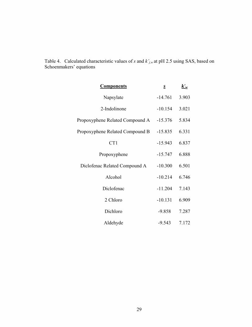
Table 4. Calculated characteristic values of s and k’j,w at pH 2.5 using SAS, based on Schoenmakers’ equations

Components s k'w

Napsylate -14.761 3.903

2-Indolinone -10.154 3.021

Propoxyphene Related Compound A -15.376 5.834

Propoxyphene Related Compound B -15.835 6.331

CT1 -15.943 6.837

Propoxyphene -15.747 6.888

Diclofenac Related Compound A -10.300 6.501

Alcohol -10.214 6.746

Diclofenac -11.204 7.143

2 Chloro -10.131 6.909

Dichloro -9.858 7.287

Aldehyde -9.543 7.172

30

ln k' vs Organic Fraction

-3.0

-2.0

-1.0

0.0

1.0

2.0

3.0

4.0

5.0

6.0

0.1 0.15 0.2 0.25 0.3 0.35 0.4 0.45 0.5 0.55 0.6

Organic Fraction

ln k

'

2 Indolinone Prop Rel Cmpd A Prop Rel Cmpd B CT1 Propoxyphene Diclo Rel Cmpd AAlcohol 2 Chloro Dicloro Aldehyde Diclofenac Napsylate

Figure 8. Plot of ln k’ vs. organic fraction at pH 2.5 based on Schoenmakers’ equations

31

minutes required a percent organic of greater than 32%. However, if the organic

composition is too high, some peaks may elute with or too close to the solvent front.

Based upon Figure 8, there are several solutes that may coelute at most organic

compositions. By examining the chromatogram of the gradient run, it was determined

whether isocratic separation was feasible or not. When the ratio of the absolute

difference of the retention time of the most retained solute and least retained solute to the

linear gradient time is less than 0.25, an isocratic method is the method of choice and

there is no need for the development of a gradient method. When this ratio is greater than

0.25, but less than 0.40, development of an isocratic method may be feasible. If the ratio

is greater than 0.4, an isocratic separation is impossible and the development of a gradient

method will be required. A gradient run with 1.2% per minute slope in which the ratio is

0.74 can be observed in Figure 9. From this data, it can be predicted that an isocratic

method, using acetonitrile in the mobile phase with the X-Terra 3.5 µm particle size

column, cannot separate all components.

In order to demonstrate the reliability of these predictive methodologies, an

isocratic run was performed. Based on Figure 8, the best isocratic run was determined to

be 40% acetonitrile. An isocratic run was performed using an X-Terra MS 150 x 4.6

mm, 3.5 µm particle size column with mobile phase composed of 50 mM potassium

phosphate buffer, pH 2.5:acetonitrile in a volumetric ratio of 60:40. The flow rate was

1.0 mL/minute and 50 µL of a mixture solution and all independent solutions were

injected and collected at 217 nm. Figure 10 shows the resulting chromatogram. The

predicted retention times were compared to the experimental retention times (Table 5)

and were observed to be similar. However, as predicted by the plot in Figure 8, the

32

m

V

40.00

45.00

50.00

55.00

60.00

65.00

70.00

75.00

80.00

85.00

90.00

95.00

100.00

105.00

110.00

115.00

120.00

Minutes5.00 10.00 15.00 20.00 25.00 30.00 35.00 40.00

2 in

doli

none

- 7.

910

Nap

syla

te -

8.35

9

Prop

Rel

Cm

pd A

- 16

.284

Prop

Rel

Cm

pd B

- 18

.065

CT

1 - 2

0.29

4Pr

opox

yphe

ne -

20.7

59

Dic

lo R

el C

mpd

A -

29.7

43

Dic

lofe

nac

- 31.

707

2 ch

loro

- 33

.357

Dic

hlor

o - 3

7.33

8A

ldeh

yde

- 37.

616

Figure 9. Chromatogram of a mixture solution, 1.2% per minute gradient slope using acetonitrile as organic modifier

33

m

V

50.00

60.00

70.00

80.00

90.00

100.00

110.00

120.00

Minutes0.00 1.00 2.00 3.00 4.00 5.00 6.00

Nap

syla

te -

1.84

3

2 in

dolin

one

- 2.2

39

Pro

p R

el C

mpd

A -

2.68

2

Pro

p R

el C

mpd

B -

3.00

6

CT1

- 3.

723

Pro

poxy

phen

e - 3

.912

mV

50.00

55.00

60.00

65.00

70.00

75.00

80.00

85.00

90.00

95.00

100.00

105.00

110.00

115.00

120.00

Minutes0.00 5.00 10.00 15.00 20.00 25.00 30.00 35.00 40.00 45.00 50.00 55.00

Nap

syla

te -

1.84

32

indo

linon

e - 2

.239

Pro

p R

el C

mpd

A -

2.68

2P

rop

Rel

Cm

pd B

- 3.

006

CT1

- 3.

723

Pro

poxy

phen

e - 3

.912

Dic

lo R

el C

mpd

A -

16.0

14

Dic

lofe

nac

- 21.

297

2 ch

loro

- 26

.903

Dic

hlor

o - 4

8.64

0

Figure 10. Chromatogram of mixture solution for isocratic method using 40:60, acetonitrile:phosphate buffer, pH 2.5, as the mobile phase

34

Table 5. Predicted retention times versus actual retention times for isocratic separation using a mobile phase buffer, pH 2.5 and acetonitrile in a volumetric ratio of 60:40

Component

Measured Retention Time

(minutes)

Predicted Retention Time

(minutes)

Napsylate 1.8 1.8

2-Indolinone 2.3 2.2

Propoxyphene Related Compound A 2.8 2.7

Propoxyphene Related Compound B 3.2 3.2

CT1 3.9 4.1

Propoxyphene 4.1 4.5

Diclofenac Related Compound A 16.4 18.8

Alcohol 25.8 24.3

Diclofenac 21.7 24.4

2 Chloro 28.1 29.3

Dichloro 47.4 46.6

Aldehyde 48.2 47.1

35

diclofenac and alcohol peaks, and the dichloro and aldehyde peaks coeluted and many

peaks eluted too close to the solvent front. Thus, adequate resolution was not achieved.

Because the isocratic method using acetonitrile and the aforementioned isocratic

conditions was not possible for this system, a gradient method was developed.

There are many advantages of gradient methods such as improving separation,

shortening the run time and improving the sensitivity. A gradient run was performed

using an X-Terra MS 150 x 4.6 mm, 3.5 µm particle size column with mobile phase A

composed of 50 mM potassium phosphate buffer, pH 2.5:acetonitrile in a volumetric ratio

of 90:10 and mobile phase B composed of 50 mM potassium phosphate buffer, pH

2.5:acetonitrile in a volumetric ratio of 35:65. The flow rate was 1.0 mL/minute and 20

µL of a mixture solution and all independent solutions were injected and collected at 217

nm. A linear gradient with a slope of 1.2% per minute (5% to 95% mobile phase B in 40

minutes) was implemented. As noted in the chromatogram shown in Figure 11, the

diclofenac and alcohol peaks coeluted. The gradient could not be further optimized to

decrease the run time. There was no empty space in the beginning or the end of the run

and all solutes were scattered during the run time.

Optimization of pH

Understanding the selectivity of pH on different solutes is beneficial when

optimizing the analytical method. The pH effects were summarized by plotting, ln k’

versus pH when the organic percentage was held constant at 35% (Figure 12). From this

graph, the pH selectivity can be observed. It was demonstrated that the retention times of

basic solutes increased as the pH is increased. The retention time of diclofenac, which is

an acidic solute, decreased with the increasing pH. Each solute’s sensitivity to pH varies

36

mV

40.00

45.00

50.00

55.00

60.00

65.00

70.00

75.00

80.00

85.00

90.00

95.00

100.00

105.00

110.00

115.00

120.00

Minutes5.00 10.00 15.00 20.00 25.00 30.00 35.00 40.00

2 in

doli

none

- 7.

910

Nap

syla

te -

8.35

9

Prop

Rel

Cm

pd A

- 16

.284

Prop

Rel

Cm

pd B

- 18

.065

CT

1 - 2

0.29

4Pr

opox

yphe

ne -

20.7

59

Dic

lo R

el C

mpd

A -

29.7

43

Dic

lofe

nac

- 31.

707

2 ch

loro

- 33

.357

Dic

hlor

o - 3

7.33

8A

ldeh

yde

- 37.

616

Figure 11. Chromatogram of mixture solution, 1.2% per minute gradient slope, acetonitrile as organic modifier in mobile phase, pH 2.5

Alcohol

37

ln k' vs pH

-3

-2

-1

0

1

2

3

4

2 3 4 5 6 7 8 9

pH

ln k

'

Napsylate 2 Indolinone Prop Rel Cmpd A Prop Rel Cmpd B CT1 PropoxypheneDiclo Rel Cmpd A Alcohol Diclofenac 2 Chloro Dichloro Aldehyde

ln k' vs pH

0

1

2

3

4

2 3 4 5 6 7 8 9

pH

ln k

'

Alcohol Diclofenac

Figure 12. A plot of ln k’ vs. pH when the percentage of organic in the mobile phase is held at 35%

38

which allowed the optimum pH to be selected. The selectivity of the diclofenac is

different than other components. This was due to the pKa of diclofenac being lower than

that of the other compounds. Diclofenac is a carboxylic acid and its pKa is about 4.0. If

the pH is lower than 4.0, diclofenac is mainly non-ionic; if the pH is higher that 4.0,

diclofenac is mainly ionized. Ionized forms are not retained on the non-polar reversed

phase column as well as non-ionic forms. Therefore, decreased retention time of

diclofenac by increased pH was expected.

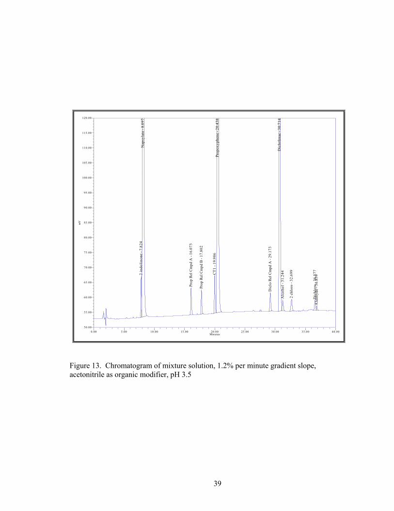
By referring to the pH selectivity of diclofenac and alcohol in Figure 12,

increasing the pH of the mobile phase increases the retention time of alcohol and

decreases the retention time of diclofenac. The pH of the mobile phase was increased to

3.5 and the resulting chromatogram is shown in Figure 13. By making a simple

adjustment of pH to the mobile phase, resolution of all solutes was obtained. A

developed gradient method implements an X-Terra MS 150 x 4.6 mm, 3.5 µm particle

size column with mobile phase A as 50 mM potassium phosphate buffer, pH

3.5:acetonitrile in a volumetric ratio of 90:10 and mobile phase B 50 mM potassium

phosphate buffer, pH 3.5:acetonitrile in a volumetric ratio of 35:65 with a gradient slope

of 1.2% per minute (5% to 95% mobile phase B in 40 minutes). The flow rate was 1.0

mL per minute with an injection volume of 20 µL. The wavelength was set at 217 nm for

the first 24 minutes then switched to 254 nm at 25 minutes. The wavelength was changed

after 25 minutes to 254 nm to decrease the absorption of gradient peaks and to optimize

the absorption of diclofenac and diclofenac related substances.

Isoelutropic Binary Method Development

A gradient method for assay and impurities was developed in which all solutes

39

mV

50.00

55.00

60.00

65.00

70.00

75.00

80.00

85.00

90.00

95.00

100.00

105.00

110.00

115.00

120.00

Minutes0.00 5.00 10.00 15.00 20.00 25.00 30.00 35.00 40.00

2 in

doli

none

- 7.

824

Nap

syla

te -

8.09

7

Prop

Rel

Cm

pd A

- 16

.073

Prop

Rel

Cm

pd B

- 17

.802

CT

1 - 1

9.98

6Pr

opox

yphe

ne -

20.4

38

Dic

lo R

el C

mpd

A -

29.1

73

Dic

lofe

nac

- 30.

714

Alc

ohol

- 31

.244

2 ch

loro

- 32

.699

Dic

hlor

o - 3

6.57

7A

ldeh

yde

- 36.

859

Figure 13. Chromatogram of mixture solution, 1.2% per minute gradient slope, acetonitrile as organic modifier, pH 3.5

40

were adequately separated. However, an isocratic method was preferred because it has

better reproducibility, less complications and clean chromatography which is free from

gradient artifacts. By changing the organic solvent to methanol, the selectivities of the

peaks were affected and provide different separation. It is known that methanol will

cause a greater back pressure on the system due to the higher viscosity of methanol/buffer

compared to acetonitrile/buffer. Therefore, the column was changed to 5 µm particle size

which would decrease the pressure by about one half compared with the 3.5 µm particle

size column. Theoretically, the particle size should not affect the retention time of solute.

However, practically, it is difficult to reproduce the exact properties of the packing

material. Therefore, the previous experiment performed to predict the retention times

may not be accurate. In order to accurately predict the retention time behavior on the 5

µm column, the Schoenmakers’ two gradient approach was applied using acetonitrile.

Two gradient runs, each with different gradient slopes were performed. The

experiments employed the X-Terra MS 150 x 4.6 mm, 5 µm particle size column.

Because the particle size was increased to 5 µm, it was possible to increase the flow rate

to 2.0 mL/min and obtain an acceptable back pressure. Mobile phase A was buffer, pH

3.5 and acetonitrile in a volumetric ratio of 90:10 and mobile phase B was buffer, pH 3.5

and acetonitrile in a volumetric ratio of 35:65. The first gradient slope was 2.5% per

minute or 5% to 95% mobile phase B in 20 minutes and the second gradient slope was

1.2% per minute or 5% to 95% mobile phase B in 40 minutes. After the completion of

the gradient, the mobile phase remained at the final composition for at least 10 minutes to

ensure all solutes elute during the run time. All solutes eluted before the completion of

the gradient. The retention time of each solute was measured for each gradient run. The

41

slope, s and capacity factor in pure weak solvent (kj,w) were calculated by SAS (Table 6)

and a plot of ln k’j versus the fraction of organic (φ ) was established (Figure 14).

From the plot, 34% acetonitrile was selected as the optimum amount of

acetonitrile in the mobile phase. An isocratic run was performed using an X-Terra RP

C18 150 x 4.6 mm, 5 µm particle size with a mobile phase composition 50 mM

potassium phosphate buffer, pH 3.5 and acetonitrile in a volumetric ratio of 66:34 with a

flow rate of 2.0 mL/minute. The column temperature was at ambient laboratory

conditions and 20 µL was injected. The resulting chromatogram is shown in Figure 15.

As expected by the predictions from the plot in Figure 14 and as observed from studies

using the 3.5 µm particle size column, diclofenac coelutes with the alcohol and 2-chloro

impurities. Because separation could not be achieved with acetonitrile, the organic

modifier was changed to methanol. The isoelutropic solution based on Herman's cubic

equation (Equation 18) was used to determine an amount of methanol equivalent to 34%

acetonitrile. It was determined that 34% acetonitrile is equivalent to 44% methanol. An

isocratic run using 44% methanol as the organic modifier was performed using the X-

Terra RP C18 150 x 4.6 mm, 5 µm particle size with a mobile phase composition 50 mM

potassium phosphate buffer, pH 3.5 and methanol in a volumetric ratio of 56:44 with a

flow rate of 2.0 mL/minute. The column temperature was at ambient laboratory

conditions and 20 µL was injected. The resulting chromatogram is shown in Figure 16.

A comparison of the two chromatograms is shown in Figure 17. The run time of

the 44% methanol run was significantly longer than the 34% acetonitrile run that was

42

Table 6. Calculated characteristic values of s and k’j,w at pH 2.5 using SAS, based on Schoenmakers’ equations

Components s k'j,w

Napsylate -15.462 3.712

2-Indolinone -10.298 2.867

Propoxyphene Related Compound A -15.257 5.473

Propoxyphene Related Compound B -16.392 6.081

CT1 -18.160 7.043

Propoxyphene -17.592 6.941

Diclofenac Related Compound A -12.150 6.914

Alcohol -12.235 7.493

Diclofenac -12.811 7.691

2 Chloro -12.161 7.471

Dichloro -11.844 8.002

Aldehyde -11.978 8.000

43

ln k' vs. Organic Fraction

-3

-2

-1

0

1

2

3

4

5

6

0.1 0.15 0.2 0.25 0.3 0.35 0.4 0.45 0.5 0.55 0.6

Organic Fraction

ln k

'

2-Indolinone Prop Rel Cmpd A Prop Rel Cmpd B CT1 Propoxyphene Diclo Rel Cmpd AAlcohol 2 Chloro Dichloro Aldehyde Diclofenac Nap

Figure 14. A plot of ln k’ vs. organic fraction, pH 3.5, 5 µm particle size column

44

AU

52.00

54.00

56.00

58.00

60.00

62.00

64.00

66.00

68.00

70.00

72.00

74.00

76.00

78.00

80.00

82.00

84.00

86.00

88.00

90.00

Time (minutes)0.00 1.00 2.00 3.00 4.00 5.00 6.00

2 In

dolin

one

- 1.4

20

Pro

p R

el C

mpd

A -

2.02

2

Pro

p R

el C

mpd

B -

2.29

8

CT1

- 3.

001

Pro

pxyp

hene

- 3.

159

3.71

3

A

U

52.00

54.00

56.00

58.00

60.00

62.00

64.00

66.00

68.00

70.00

72.00

74.00

Time (minutes)0.00 5.00 10.00 15.00 20.00 25.00 30.00 35.00 40.00 45.00 50.00 55.00 60.00

2 In

dolin

one

- 1.4

20P

rop

Rel

Cm

pd A

- 2.

022

Pro

p R

el C

mpd

B -

2.29

8C

T1 -

3.00

1P

ropx

yphe

ne -

3.15

93.

713

7.29

89.

047

9.76

2 Dic

lo R

el C

mpd

A -

13.8

3814

.577

Dic

lofe

nac

- 24.

471

32.7

97

Ald

ehyd

e - 4

8.85

8

Dic

hlor

o - 5

3.03

7

Figure 15. Chromatogram of a mixture solution from an isocratic run using 34% acetonitrile, pH 3.5

45

AU

52.00

54.00

56.00

58.00

60.00

62.00

64.00

66.00

68.00

70.00

72.00

74.00

76.00

78.00

80.00

82.00

84.00

86.00

88.00

90.00

Time (minutes)0.00 1.00 2.00 3.00 4.00 5.00 6.00

2.11

92.

288

Pro

p R

el C

mpd

A -

2.70

7

Pro

p R

el C

mpd

B -

3.04

6

Pro

poxy

phen

e - 4

.634

A

U

52.00

54.00

56.00

58.00

60.00

62.00

64.00

66.00

68.00

70.00

72.00

74.00

Time (minutes)0.00 10.00 20.00 30.00 40.00 50.00 60.00 70.00 80.00

2.11

92.

288

Pro

p R

el C

mpd

A -

2.70

7P

rop

Rel

Cm

pd B

- 3.

046

Pro

poxy

phen

e - 4

.634

Dic

lo R

el C

mpd

A -

13.7

35

28.7

18 Alc

ohol

- 32

.470

Dic

lofe

nac

- 41.

504

Ald

ehyd

e - 7

3.42

3

Figure 16. Chromatogram of a mixture solution, isocratic method using 44% methanol in the mobile phase, pH 3.5

46

predicted by Herman’s isoelutropic expression. Therefore, the strength of methanol

equivalent to 34% acetonitrile was determined by Schoenmakers’ isoelutropic solution

(Equation 16). According to Schoenmakers’ expression, 34% acetonitrile is equivalent to

47% methanol. An isocratic run using 47% methanol as the organic modifier was

performed using the X-Terra RP C18 150 x 4.6 mm, 5 µm particle size with a mobile

phase composition 50 mM potassium phosphate buffer, pH 3.5 and methanol in a

volumetric ratio of 53:47 with a flow rate of 2.0 mL/minute. The column temperature

was at ambient laboratory conditions and 20 µL was injected. The resulting

chromatogram is shown in Figure18. The similar run times of the 34% acetonitrile

isocratic run and the 47% methanol isocratic run can be seen in Figure 19.

Schoenmakers’ prediction more accurately estimated the isoelutropic equivalence

compared to Herman’s. The separation of alcohol and diclofenac was achieved from the

different selectivity of methanol. However, CT1 and propoxyphene coelute when using

methanol as the organic modifier. Because an isocratic separation was not achievable

using acetonitrile or methanol, a ternary separation was evaluated.

Applying Mixtures of Organic Solvents

According to the mixture design, for a ternary system, at least three experiments

must be performed to determine the composition of mobile phase that would provide an

optimum separation of all peaks (Figure 20). The binary systems were performed

previously for acetonitrile and methanol. Using the mixture design, a study was

performed using a ternary system (mixture of acetonitrile, methanol and phosphate

buffer) at a point between the optimum binary conditions of methanol and acetonitrile.

An isocratic run was performed using the X-Terra RP C18 150 x 4.6 mm, 5 µm particle

47

AU

55.00

60.00

65.00

70.00

75.00

80.00

85.00

90.00

2 In

dolin

one

- 1.4

20

Pro

p R

el C

mpd

A -

2.02

2

Pro

p R

el C

mpd

B -

2.29

8

CT1

- 3.

001

Pro

pxyp

hene

- 3.

159

3.71

3

AU

55.00

60.00

65.00

70.00

75.00

80.00

85.00

90.00

Time (minutes)0.00 1.00 2.00 3.00 4.00 5.00 6.00

2.11

7

Pro

p R

el C

mpd

A -

2.68

3

Pro

p R

el C

mpd

B -

3.01

6

Pro

poxy

phen

e - 4

.581

34% Acetonitrile

44% Methanol

AU

55.00

60.00

65.00

70.00

75.00

2 In

dolin

one

- 1.4

20Pr

op R

el C

mpd

A -

2.02

2Pr

op R

el C

mpd

B -

2.29

8C

T1 -

3.00

1Pr

opxy

phen

e - 3

.159

3.71

3

7.29

89.

047

9.76

2

Dic

lo R

el C

mpd

A -

13.8

3814

.577

Dic

lofe

nac

- 24.

471

32.7

97 Ald

ehyd

e - 4

8.85

8

Dic

hlor

o - 5

3.03

7

AU

55.00

60.00

65.00

70.00

75.00

Time (minutes)0.00 10.00 20.00 30.00 40.00 50.00 60.00 70.00 80.00

2.11

7Pr

op R

el C

mpd

A -

2.68

3Pr

op R

el C

mpd

B -

3.01

6Pr

opox

yphe

ne -

4.58

1

Dic

lo R

el C

mpd

A -

13.5

28

2 C

hlor

o - 1

8.67

4

27.9

45

Alc

ohol

- 31

.826 Dic

lofe

nac

- 40.

502

Dic

hlor

o - 5

6.39

6

Ald

ehyd

e - 7

1.90

0

34% Acetonitrile

44% Methanol

Figure 17. Chromatogram overlay of mixture solution for isocratic runs using 34% acetonitrile and 44% methanol

48

AU

52.00

54.00

56.00

58.00

60.00

62.00

64.00

66.00

68.00

70.00

72.00

74.00

76.00

78.00

80.00

82.00

84.00

86.00

88.00

90.00

Time (minutes)0.00 1.00 2.00 3.00 4.00 5.00 6.00

2.04

2P

rop

Rel

Cm

pd A

- 2.

208

Pro

p R

el C

mpd

B -

2.41

3

Pro

poxy

phen

e - 3

.441

AU

52.00

54.00

56.00

58.00

60.00

62.00

64.00

66.00

68.00

70.00

72.00

74.00

Time (minutes)0.00 5.00 10.00 15.00 20.00 25.00 30.00 35.00 40.00 45.00 50.00

2.04

2P

rop

Rel

Cm

pd A

- 2.

208

Pro

p R

el C

mpd

B -

2.41

3P

ropo

xyph

ene

- 3.4

41

Dic

lo R

el C

mpd

A -

9.74

5

2 C

hlor

o - 1

3.23

2

19.4

70

Alc

ohol

- 22

.050

Dic

lofe

nac

- 27.

052

Dic

hlor

o - 3

8.64

0

Ald

ehyd

e - 4

7.22

3

Figure 18. Chromatogram of a mixture solution, 47% methanol

49

AU

55.00

60.00

65.00

70.00

75.00

80.00

85.00

90.00

2 In

dolin

one

- 1.4

20

Pro

p R

el C

mpd

A -

2.02

2

Pro

p R

el C

mpd

B -

2.29

8

CT1

- 3.

001

Pro

pxyp

hene

- 3.

159

3.71

3

AU

55.00

60.00

65.00

70.00

75.00

80.00

85.00

90.00

Time (minutes)0.00 1.00 2.00 3.00 4.00 5.00 6.00

2.04

2P

rop

Rel

Cm

pd A

- 2.

208

Pro

p R

el C

mpd

B -

2.41

3

Pro

poxy

phen

e - 3

.441

34% Acetonitrile

47% Methanol

AU

55.00

60.00

65.00

70.00

75.00

2 In

dolin

one

- 1.4

20Pr

op R

el C

mpd

A -

2.02

2Pr

op R

el C

mpd

B -

2.29

8C

T1 -

3.00

1Pr

opxy

phen

e - 3

.159

3.71

37.

298

9.04

79.

762

Dic

lo R

el C

mpd

A -

13.8

3814

.577

Dic

lofe

nac

- 24.

471

32.7

97 Ald

ehyd

e - 4

8.85

8

Dic

hlor

o - 5

3.03

7

AU

55.00

60.00

65.00

70.00

75.00

Time (minutes)0.00 10.00 20.00 30.00 40.00 50.00 60.00 70.00 80.00

2.04

2Pr

op R

el C

mpd

A -

2.20

8Pr

op R

el C

mpd

B -

2.41

3Pr

opox

yphe

ne -

3.44

1

Dic

lo R

el C

mpd

A -

9.74

52

Chl

oro

- 13.

232

19.4

70 Alc

ohol

- 22

.050

Dic

lofe

nac

- 27.

052

Dic

hlor

o - 3

8.64

0

Ald

ehyd

e - 4

7.22

3

34% Acetonitrile

47% Methanol

Figure 19. Chromatogram overlay of mixture solution at 34% acetonitrile and 47% methanol.

50

Figure 20. Mixture design model for ternary mobile phase

ACN 34%

MeOH 47%

1 3 212%MeOH/ 26% ACN

THF

51

size with a mobile phase composition 50 mM potassium phosphate buffer, pH 3.5,

methanol and acetonitrile in a volumetric ratio of 62:12:26 with a flow rate of 2.0

mL/minute. The column temperature was at ambient laboratory conditions and 20 µL

injections of samples were performed. The resulting chromatogram is shown in Figure

21.

The retention time of each peak was measured and recorded for each mobile

phase, binary with acetonitrile, binary with methanol and ternary with acetonitrile and

methanol. The natural logarithms of the capacity factor for each solute (ln k’j) were

calculated at each different composition of mobile phase. Using the ln k’j , the three

constants in equation 26, a1, a2, a1,2 were calculated.

212,12211'ln xxaxaxak ++= (26)

After inserting these constants into Equation 26, the optimum mobile phase was

calculated by iterative calculation at different compositions of acetonitrile (x1) and

methanol (x2) to determine which composition would give the greatest difference in

retention time for critical pairs.

Using the same approach, the resolutions (R) at different compositions of

acetonitrile (x1) and methanol (x2) were also determined. The resolutions between all

successively eluting peaks were measured and recorded for each mobile phase, binary

with acetonitrile, binary with methanol and ternary with acetonitrile and methanol. Using

the resolutions, the three constants in equation 27, a’1, a’2, a’1,2 were calculated.

212,12211 ''' xxaxaxaR ++= (27)

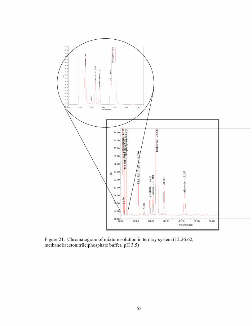
52

AU

52.00

54.00

56.00

58.00

60.00

62.00

64.00

66.00

68.00

70.00

72.00

74.00

76.00

78.00

80.00

82.00

84.00

86.00

88.00

90.00

Time (minutes)0.00 1.00 2.00 3.00 4.00 5.00 6.00

2 In

dolin

one

- 1.4

68

1.97

0

Pro

p R

el C

mpd

A -

2.31

3

Pro

p R

el C

mpd

B -

2.67

3

CT1

- 3.

629

Pro

poxy

phen

e - 3

.821

AU

52.00

54.00

56.00

58.00

60.00

62.00

64.00

66.00

68.00

70.00

72.00

74.00

Time (minutes)0.00 10.00 20.00 30.00 40.00 50.00 60.00

2 In

dolin

one

- 1.4

681.

970

Prop

Rel

Cm

pd A

- 2.

313

Prop

Rel

Cm

pd B

- 2.

673

CT1

- 3.

629

Prop

oxyp

hene

- 3.

821

Dic

lo R

el C

mpd

A -

11.7

80

15.4

04

2 C

hlor

o - 1

9.21

3A

lcoh

ol -

21.3

04D

iclo

fena

c - 2

3.82

0

28.5

06

Ald

ehyd

e - 4

2.05

7

Figure 21. Chromatogram of mixture solution in ternary system (12:26:62, methanol:acetonitrile:phosphate buffer, pH 3.5)

53

After inserting these constants into Equation 27, the optimum mobile phase was

calculated by iterative calculation at different compositions of acetonitrile (x1) and

methanol (x2) to determine which composition gives the greatest resolution of critical

pairs.

The optimum ternary composition of mobile phase using ln k’ or resolution was

predicted to be methanol, acetonitrile and phosphate buffer in a volumetric ratio of

7:29:64. An isocratic run was performed using the X-Terra RP C18 150 x 4.6 mm, 5 µm

particle size with a mobile phase composed of methanol, acetonitrile and phosphate

buffer, pH 3.5 in a volumetric ratio of 7:29:64 with a flow rate of 2.0 mL/minute. The

column temperature was at ambient laboratory conditions and 20 µL injections of

samples were performed. The resulting chromatogram is shown in Figure 22.

Table 7 and 8 compare the calculated resolutions/retention times with actual

resolutions and retention times based on the polynomial expression utilized in Equation

26. As observed in Figure 22, all process and degradation impurities have adequate

resolution for quantitation. This systematic and mathematical approach demonstrated an

acceptable analytical method for the assay of propoxyphene, diclofenac and all related

process and degradation impurities.

Column Temperature Optimization Although an isocratic ternary method was developed which separated all in-

process and degradation products, and since the 5 µm column behaved differently than

the 3.5 µm column, it was desired to simplify the method to one solvent for finished

product testing. In finished product testing, it is not necessary to quantitate in-process

impurities. Therefore, separation is not needed for dichloro and 2-chloro. An isocratic

54

AU

55.00

60.00

65.00

70.00

75.00

80.00

85.00

90.00

95.00

100.00

Time (minutes)0.00 1.00 2.00 3.00 4.00 5.00 6.00

Nap

syla

te -

1.14

8

2 In

dolin

one

- 1.4

69

2.02

5

Pro

p R

el C

mpd

A -

2.30

6

Pro

p R

el C

mpd

B -

2.67

4

CT1

- 3.

621

Pro

poxy

phen

e - 3

.813

AU

55.00

60.00

65.00

70.00

75.00

80.00

85.00

90.00

95.00

100.00

105.00

110.00

Time (minutes)0.00 5.00 10.00 15.00 20.00 25.00 30.00 35.00 40.00 45.00 50.00 55.00

Nap

syla

te -

1.14

82

Indo

linon

e - 1

.469

2.02

5Pr

op R

el C

mpd

A -

2.30

6Pr

op R

el C

mpd

B -

2.67

4C

T1 -

3.62

1Pr

opox

yphe

ne -

3.81

3

12.9

06

15.7

18 2 C

hlor

o - 2

1.86

7A

lcoh

ol -

23.1

40D

iclo

fena

c - 2

5.14

8

31.3

92

Ald

ehyd

e - 4

6.65

4D

ichl

oro

- 48.

016

Figure 22. Chromatogram of mixture solution for optimal isocratic ternary system

55

Table 7. Resolution measurements for binary systems with acetonitrile and methanol and ternary system of acetonitrile and methanol

Successive Components

Calculated Resolution

Measured Resolution

Napsylate/2-Indolinone 2.1 1.7

2-Indolinone/Prop Rel Cmpd A 5.5 5.8

Prop Rel Cmpd A/Prop Rel Cmpd B 2.0 2.1

Prop Rel Cmpd B/CT1 4.4 4.7

CT1/ Propoxyphene 0.7 0.7

Propoxyphene/Diclo Rel Cmpd A 19.7 19.7

Diclo Rel Cmpd A/2 Chloro 10.9 11.3

2 Chloro/Alcohol 1.4 1.3

Alcohol/Diclofenac 1.5 1.8

Diclofenac/Unknown Impurity 4.6 4.8

Unknown Impurity/Aldehyde 8.5 8.2

Aldehyde/Dichloro 1.0 1.0

56

Table 8. Retention time measurements for binary systems with acetonitrile and methanol and ternary system of acetonitrile and methanol

Component

Calculated Retention Time

(minutes)

Measured Retention Time

(minutes)

2-Indolinone 1.5 1.5

Propoxyphene Related Compound A 2.2 2.3

Propoxyphene Related Compound B 2.5 2.7

CT1 3.4 3.6

Propoxyphene 3.6 3.8

Diclofenac Related Compound A 12.6 12.9

2 Chloro 21.0 21.9

Alcohol 22.5 23.1

Diclofenac 24.2 25.1

Unknown Impurity 30.2 31.4

Aldehyde 44.5 46.7

Dichloro 46.0 48.0

57

run was performed using the X-Terra RP C18 150 x 4.6 mm, 5 µm particle size with a

mobile phase composed of 50 mM potassium phosphate buffer, pH 3.5 and acetonitrile in

a volumetric ratio of 66:34 with a flow rate of 2.0 mL/minute. The column temperature

was at ambient laboratory conditions and 20 µL injections of samples were performed.

The resulting chromatogram is shown in Figure 15. The measured retention times were

similar to the retention times predicted from the plot in Figure 14 (Table 9).

Because diclofenac and alcohol still coelute, the temperature of the column was

evaluated. The column temperature often aids in the separation of components because of

different heat of enthalpy values (∆H) for each solute. The temperature effects were

studied by injecting solutes using different column temperatures while all other variables

were held constant. An isocratic run was performed using the X-Terra RP C18 150 x 4.6

mm, 5 µm particle size with a mobile phase composed of 50 mM potassium phosphate

buffer, pH 3.5 and acetonitrile in a volumetric ratio of 66:34 with a flow rate of 2.0

mL/minute and 20 µL injection volume. The resulting chromatograms are shown in

Figures 23 and 24.

The separation of the alcohol and diclofenac, and the CT1 and propoxyphene

improved as the temperature increased. By measuring the retention times of each solute

at each temperature, the plot of ln k’ vs. 1/T is observed in Figure 25. Using the data at

different temperatures, ∆H’s in equilibrium between the mobile phase and the stationary

phase, were calculated using the following equation (Table 10).

(28)

Constantln +∆−

=RT

Hk

58

Table 9. Predicted retention times versus actual retention times for isocratic separation using a 5 µm particle size column a mobile phase buffer, pH 3.5 and acetonitrile in a volumetric ratio of 66:34

Component

Measured Retention Time

(minutes)

Predicted Retention Time

(minutes)

2-Indolinone 1.4 1.3

Propoxyphene Related Compound A 2.0 2.0

Propoxyphene Related Compound B 2.3 2.3

CT1 3.1 2.9

Propoxyphene 3.2 3.1

Diclofenac Related Compound A 14.1 14.6

Alcohol 24.8 24.7

Diclofenac 25.2 24.7

Aldehyde 50.2 44.0

59

AU

60.00

80.00

100.00

Prop

Rel

Cm

pd A

- 2.

175

Prop

Rel

Cm

pd B

- 2.

469

2.72

8

Prop

oxyp

hene

- 3.

407

CT1

- 3.

933

AU

60.00

80.00

100.00

2 In

dolin

one

- 1.3

25

Prop

Rel

Cm

pd A

- 1.

836

Prop

Rel

Cm

pd B

- 2.

074

Prop

oxyp

hene

- 2.

805

4.94

1

AU

60.00

80.00

100.00

2 In

dolin

one

- 1.2

90

Prop

Rel

Cm

pd A

- 1.

764

Prop

Rel

Cm

pd B

- 1.

987

CT1

- 2.

477

Prop

oxyp

hene

- 2.

662

4.46

6

AU

60.00

80.00

100.00

2 In

dolin

one

- 1.2

70

Prop

Rel

Cm

pd A

- 1.

718

Prop

Rel

Cm

pd B

- 1.

929

CT1

- 2.

382

Prop

oxyp

hene

- 2.

566

4.11

0

AU

60.00

80.00

100.00

Time (minutes)0.00 0.50 1.00 1.50 2.00 2.50 3.00 3.50 4.00 4.50 5.00

2 In

dolin

one

- 1.2

38

Prop

Rel

Cm

pd A

- 1.

645

Prop

Rel

Cm

pd B

- 1.

839

CT1

- 2.

241

Prop

oxyp

hene

- 2.

414

3.72

1

5C

45C

50C

55C

60C

Figure 23. Chromatogram of mixture solution from an isocratic run having a mobile phase of 34:66 acetonitrile:buffer, pH 3.5 at various column temperatures from 0-5 minutes

60

AU

60.00

80.00

100.00

Prop

Rel

Cm

pd A

- 2.

175

Prop

Rel

Cm

pd B

- 2.

469

2.72

8Pr

opox

yphe

ne -

3.40

7C

T1 -

3.93

3

10.7

49 11.3

92

Dic

lo R

el C

mpd

A -

18.3

34

21.8

42

2 C

hlor

o - 3

4.56

4

Dic

lofe

nac

- 36.

997

50.5

23

Ald

ehyd

e - 7

0.18

3

Dic

hlor

o - 7

9.28

8

AU

60.00

80.00

100.00

2 In

dolin

one

- 1.3

25Pr

op R

el C

mpd

A -

1.83

6Pr

op R

el C

mpd

B -

2.07

4Pr

opox

yphe

ne -

2.80

5

4.94

1

7.09

4 7.72

29.

200

Dic

lo R

el C

mpd

A -

10.0

18

Dic

lofe

nac

- 14.

966

2 C

hlor

o - 1

6.89

6

19.8

32 Ald

ehyd

e - 3

1.32

6D

ichl

oro

- 32.

713

AU

60.00

80.00

100.00

2 In

dolin

one

- 1.2

90Pr

op R

el C

mpd

A -

1.76

4Pr

op R

el C

mpd

B -

1.98

7C

T1 -

2.47

7 Prop

oxyp

hene

- 2.

662

4.46

6

6.60

9 7.20

28.

232

Dic

lo R

el C

mpd

A -

9.24

4

Dic

lofe

nac

- 13.

330

Alc

ohol

- 14

.204

2 C

hlor

o - 1

5.41

5

17.6

68 Ald

ehyd

e - 2

8.26

8D

ichl

oro

- 29.

268

AU

60.00

80.00

100.00

2 In

dolin

one

- 1.2

70Pr

op R

el C

mpd

A -

1.71

8Pr

op R

el C

mpd

B -

1.92

9C

T1 -

2.38

2 Prop

oxyp

hene

- 2.

566

4.11

0

6.21

2 6.77

07.

464

Dic

lo R

el C

mpd

A -

8.60

1

Dic

lofe

nac

- 11.

984

Alc

ohol

- 12

.932

2 C

hlor

o - 1

4.15

2

15.8

56 Ald

ehyd

e - 2

5.65

1D

ichl

oro

- 26.

190

AU

60.00

80.00

100.00

Time (minutes)0.00 10.00 20.00 30.00 40.00 50.00 60.00 70.00 80.00

2 In

dolin

one

- 1.2

38Pr

op R

el C

mpd

A -

1.64

5Pr

op R

el C

mpd

B -

1.83

9C

T1 -

2.24

1Pr

opox

yphe

ne -

2.41

43.

721

5.68

56.

194 6.

667

Dic

lo R

el C

mpd

A -

7.83

3

Dic

lofe

nac

- 10.

602

Alc

ohol

- 11

.510

2 C

hlor

o - 1

2.69

913

.929 A

ldeh

yde

- 22.

721

5C

45C

50C

55C

60C

Figure 24. Chromatogram of mixture solution from an isocratic run having a mobile phase of 34:66 acetonitrile:buffer, pH 3.5 at various column temperatures from 0-85 minutes

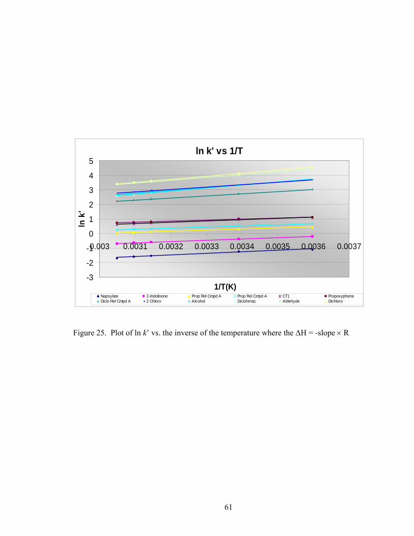
61

ln k' vs 1/T

-3

-2

-1

0

1

2

3

4

5

0.003 0.0031 0.0032 0.0033 0.0034 0.0035 0.0036 0.0037

1/T(K)

ln k

'

Napsylate 2-Indolinone Prop Rel Cmpd A Prop Rel Cmpd A CT1 PropoxypheneDiclo Rel Cmpd A 2 Chloro Alcohol Diclofenac Aldehyde Dichloro

Figure 25. Plot of ln k’ vs. the inverse of the temperature where the ∆H = -slope × R

62

Table 10. Calculated ∆H in equilibrium between the mobile phase and stationary phase

Components ∆H (kcal/mol)

Napsylate -2.127

2-Indolinone -1.771

Propoxyphene Related Compound A -1.564

Propoxyphene Related Compound B -1.505

CT1 -1.787

Propoxyphene -1.449

Diclofenac Related Compound A -2.943

Alcohol -3.742

Diclofenac -4.259

2 Chloro -3.335

Dichloro -4.048

Aldehyde -3.726

63

The negative slope multiplied by the molar gas constant gives the ∆H. If the

∆H’s are similar, the components are expected to behave similarly as temperature varies.

A greater difference in ∆H will result in a greater improvement in resolution when the

column temperature is increased.

Since the best resolution was observed at 60°C, Schoenmakers’ two gradient

system was implemented to determine the optimum mobile phase at the optimum

temperature of 60°C. The experiments utilized the X-Terra MS 150 x 4.6 mm, 5 µm

particle size column maintained at 60°C. Mobile phase A was buffer, pH 3.5 and

acetonitrile in a volumetric ratio of 90:10 and mobile phase B was buffer, pH 3.5 and

acetonitrile in a volumetric ratio of 35:65 with a flow rate of 2.0 mL/minute. The first

gradient slope was 2.5% per minute or 5% to 95% mobile phase B in 20 minutes and the

second gradient slope was 1.2% per minute or 5% to 95% mobile phase B in 40 minutes.

After the completion of the gradient, the mobile phase remained at the final composition

for at least 10 minutes to ensure all solutes elute during the run time. All solutes eluted

before the completion of the gradient. The retention time of each solute was measured

for each gradient run. The slope, s, and capacity factor in pure weak solvent (kj,w) for each

solute was calculated by SAS (Table 11) and a plot of ln k’j versus the fraction of organic

(φ ) was established (Figure 26).

The plot in Figure 26 demonstrated that 35% acetonitrile with a column

temperature of 60°C would provide adequate resolution of all degradation products.

Therefore an isocratic run was performed using the X-Terra RP C18 150 x 4.6 mm, 5 µm

particle size with a mobile phase composed of 50 mM potassium phosphate buffer, pH

64

Table 11. Calculated characteristic values of s and k’j,w at pH 3.5 and column temperature of 60°C using SAS, based on Schoenmakers’ equations

Components s k' j,w

Napsylate -19.371 3.333

2-Indolinone -14.876 2.789

Propoxyphene Related Compound A -15.917 4.828

Propoxyphene Related Compound B -16.911 5.421

CT1 -16.961 5.897

Propoxyphene -17.079 6.074

Diclofenac Related Compound A -12.121 6.122

Alcohol -11.810 6.475

Diclofenac -12.030 6.640

2 Chloro -12.858 6.725

Dichloro -11.384 7.048

Aldehyde -11.524 7.083

65

ln k' vs Organic Fraction

-1

-0.5

0

0.5

1

1.5

2

2.5

3

3.5

4

0.2 0.25 0.3 0.35 0.4

Organic Fraction

ln k

'

2 -Indolinone Prop. Rel. Cmpd A Prop. Rel. Cmpd B CT1Propoxyphene Diclo. Rel. Cmpd A Alcohol 2 ChloroDichloro Aldehyde Diclofenac Nap

Figure 26. A plot of ln k’ vs. organic fraction, pH 3.5, 5 µm particle size column at 60°C

.

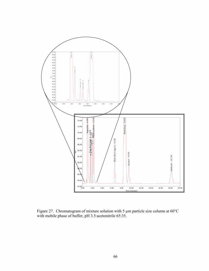
66

AU

52.00

54.00

56.00

58.00

60.00

62.00

64.00

66.00

68.00

70.00

72.00

74.00

76.00

78.00

80.00

82.00

84.00

86.00

88.00

90.00

Time (minutes)0.00 0.50 1.00 1.50 2.00 2.50 3.00 3.50 4.00

Nap

syla

te -

0.99

4

2 In

dolin

one

- 1.2

10

Prop

Rel

Cm

pd A

- 1.

557

Prop

Rel

Cm

pd B

- 1.

718

CT1

- 2.

072

Prop

oxyp

hene

- 2.

234

AU

52.00

54.00

56.00

58.00

60.00

62.00

64.00

66.00

68.00

70.00

72.00

74.00

Time (minutes)0.00 2.00 4.00 6.00 8.00 10.00 12.00 14.00 16.00 18.00 20.00

Nap

syla

te -

0.99

1Pr

op R

el C

mpd

A -

1.55

8Pr

op R

el C

mpd

B -

1.72

0C

T1 -

2.07

3Pr

opox

yphe

ne -

2.23

6

Dic

lo R

el C

mpd

A -

6.59

2

Dic

lofe

nac

- 8.6

28

Alc

ohol

- 9.

470

Ald

ehyd

e - 1

8.21

0

Figure 27. Chromatogram of mixture solution with 5 µm particle size column at 60°C with mobile phase of buffer, pH 3.5:acetonitrile 65:35.

67

Table 12. Predicted retention times vs. actual retention times for isocratic separation using a 5 µm particle size column at 60°C, a mobile phase of buffer, pH 3.5 and acetonitrile in a volumetric ratio of 65:35

Component

Measured Retention Time

(minutes)

Predicted Retention Time

(minutes)

2-Indolinone 1.2 0.8

Propoxyphene Related Compound A 1.5 1.3

Propoxyphene Related Compound B 1.7 1.3

CT1 2.0 1.5

Propoxyphene 2.2 1.7

Diclofenac Related Compound A 6.4 6.0

Diclofenac 8.3 8.1

Alcohol 9.2 9.0

Aldehyde 17.5 17.4

68

3.5 and acetonitrile in a volumetric ratio of 65:35 with a flow rate of 2.0 mL/minute and a

20 µL injection volume. The resulting chromatogram is shown in Figure 27. The

predicted retention times correlated well with the measured retention times (Table 12).

All peaks of interest were adequately separated.

Dissolution Method Development

Dissolution profiles are the often performed to demonstrate how a product may

behave in man as well as how it may behave over time. When performing dissolution

profiles with 6 to 12 tablet dissolutions, the number of samples to be tested is significant.

Therefore, it is important to develop a method with a short run time to allow the total

testing time to be efficient. A dissolution method was developed based on the plot of ln

k’ versus. organic fraction (Figure 8). From the plot, the percentage of acetonitrile in the

mobile phase can be estimated. At 45% acetonitrile, the plot predicted propoxyphene to

elute just after the solvent front at 2.9 minutes and diclofenac should elute at 14.6

minutes. As observed in Figure 12, if the pH of the mobile phase is increased, diclofenac

would have a shorter retention time and propoxyphene would have a longer retention

time which would result in a shorter run time and better separation from the solvent front.

Therefore the pH of the mobile phase was increased to 3.5. The following instrument

parameters were selected for the dissolution method.

HPLC Parameters:

Column: X-Terra MS 150 x 4.6 mm, 3.5 µm particle size Mobile Phase A: 55:45, 50 mM potassium phosphate buffer, pH 3.5:acetonitrile Flow Rate: 1.0 mL/minute Wavelength: 217 nm Injection Volume: 10 µL Temperature: Ambient

69

Dissolution Parameters: Apparatus: USP II (Paddles) Paddle Speed: 50 RPM, 250 RPM at infinity Medium: 900 mL 50 mM K2HPO4, pH 6.8 Temperature: 37.0 ± 0.5°C Pull Volume: 10 mL Pull Times: 10, 20, 30, and 45 (infinity) minutes Filter: 0.45 µm Paddles were selected since the final dosage product will be in a soft gelatin

capsule. Typically baskets are used for capsules at 100 rotations per minute and paddles

are used for tablets and soft gelatin capsules at 50 rotation per minute. The dissolution

medium is often dilute 0.1 N hydrochloric acid to mimic the aqueous environment of the

stomach. However, diclofenac is not soluble in an acidic environment and therefore, the

approximate pH of the intestine, pH 6.8, was used. The temperature of the medium was

set at the temperature of the body, 37°C. A profile was implemented to demonstrate the

release rate of each active once it comes into contact with the intestines. Immediate

release is desirable for a fast onset. Finally, a nylon filter was selected as a suitable filter

for an aqueous solution. For the HPLC parameters, the injection volume was decreased

from the assay method which would provide minimal detection of impurities for less

interference but still have an adequate area response for a robust method. Figure 28 is an

overlay of a standard solution and sample solution. Propoxyphene was well resolved

from the solvent front and diclofenac eluted in a reasonable time to give an efficient run

time. A dissolution test was performed for a research and development prototype of the

soft gelatin capsule fill solution. The results are in Table 13. As anticipated, after 10

minutes in the intestines, the active ingredients are almost completely dissolved.

70

Figure 28. Chromatogram overlay of a standard and sample solution using a mobile phase of 45:55, acetonitrile:phosphate buffer, pH 3.5.

AU

50.00

100.00

150.00

200.00

250.00

300.00

350.00

400.00

450.00

Time (minutes)0.00 2.00 4.00 6.00 8.00 10.00 12.00 14.00

Pro

p

Dic

lo

Pro

p

Dic

lo

71

Table 13. Dissolution results of a research prototype

% Diclofenac Dissolved Vessel 10 minutes 20 minutes 30 minutes 45 minutes(infinity)

1 104 104 105 105 2 106 107 106 107 3 106 106 107 107

Mean (3) 105 106 106 106 %RSD 0.9 1.5 0.9 1.1

% Propoxyphene Dissolved Vessel 10 minutes 20 minutes 30 minutes 45 minutes(infinity)

1 93 94 93 95 2 95 96 96 95 3 94 94 95 96

Mean (3) 94 95 95 95 %RSD 1.5 1.2 1.6 0.8

72

CONCLUSION

Cost and time are major factors in the development of a pharmaceutical product.

Each day saved in development may reflect in thousands of dollars in revenue for a

company. Hence, it is of extreme importance to utilize an efficient and productive

development plan for analytical to support the integrity of the drug product.

Development and optimization of a reliable and robust method for a mixture of solutes is

challenging, time consuming and labor intensive. The development time of optimal

analytical methods using a complex multi-component system for diclofenac,

propoxyphene, and their corresponding impurities was reduced using a mathematical

approach and exploring the characteristics and behaviors of the solutes. In addition, the

cost of testing the commercial product will be less as a result of one efficient analytical

assay method for label claim, impurities and backend dissolution as opposed to multiple

analytical assay methods. This in turn may be reflected in a lower cost of the product to

the consumer.

A gradient method was developed which employed a 3.5 µm particle size column.

This method was further optimized by exploring the pH effects on each solute’s behavior.

Understanding how each solute behaves for each variable is important when optimizing

the method as demonstrated with the pH. The gradient method had adequate resolution

between all components. However, an isocratic method was desired for improving the

chromatogram baseline, reproducibility and simplicity.

Using the plot of the capacity factor of each solute versus the organic fraction, it

was shown the mixture of solutes could not be separated using a binary solvent system

(buffer and acetonitrile) when the column was maintained at room temperature. Because

73

acetonitrile could not separate all components, the isoelutropic binary expression was

used to calculate the equivalent buffer-methanol composition. The equivalent strength of

buffer-methanol showed different selectivity. However, as in the case with acetonitrile,

the buffer and methanol binary system did not give successful separation of all solutes.

Because methanol and acetonitrile had different selectivity, the mixture design theory

was implemented to develop a ternary separation. By performing only three experiments,

the optimum mixture composition of the mobile phase was selected. This ternary system

resulted in adequate separation of all solutes.

Although an excellent ternary isocratic method was developed, an attempt was

made to develop an isocratic binary method by exploring the column temperature. The

characteristics of solutes varied differently with temperature. It was shown that at 60°C,

an isocratic binary system having a mobile phase composition of 35% acetonitrile and

65% buffer could separate all actives and impurities necessary for analytical testing of the

drug product.

A dissolution method was also developed using the data collected for the

development of the assay methods. Using the plot of the capacity factor of each solute

versus the organic fraction, the optimum mobile composition was determined and a

dissolution method was developed with a short run time and good separation.

This research strongly demonstrates the benefits of using systematic and

mathematical approaches when developing analytical methods for a complex mixture.

Unlike the trial-and-error approach, which has a blinding effect with variable changes,

knowing the behaviors of all the solutes allows logical directions for the development of

74

optimal analytical methods. In turn, this approach can strongly impact the final

development and provide a final product at a reduced cost to the consumer.

REFERENCES Green, J. Mark., A Practical Guide to Analytical Method Validation. Analytical

Chemistry., 1996 (68) 305A-309A. Snyder, Lloyd R., Kirkland, Joseph J., Glajch, Joseph L., Practical HPLC Method

Development, Second Edition., New York: Whiley and Sons, Inc. 1997. Crison, www.dissoltuiontech.com/Dtresour/299articles/299Crison.htm Alm, R. S., Williams, J. P., and Tiselius, A., Gradient Elution Analysis. Acta Chem.

Scand., 1952 (6) 826 Snyder, Lloyd R., High Performance Liquid Chromatography, Advances and

Prospective., CS. Horvath Ed., New York: Acedemic Press. 1980. Jandera, P. and Churacek, J., Gradient Elution in Liquid Chromatography. Elsevier

Amsterdam, The Netherlands, 1985. Schoenmakers, P. J., Billiet, H. A. H., Tijssen, R., De Galan, L., Gradient Selection in

Reverse-Phase Liquid Chromatography. Journal of Chromatography., 1978 (149) 519-537.

Schoenmakers, P. J., Billiet, H. A. H., Tijssen, R., De Galan, L., Gradient Elution

Methods for Predicting Isocratic Conditions. Journal of Chromatography., 1991 (550) 425-447.

Herman, Dave P., Billiet, Hugo A. H., De Galan, Leo, Algorithms of Correct Gradient

Scan Transfer Rule Predictions of Isocratic Retention in Reversed-Phase Liquid Chromatography. Journal of Chromatography. 1989 (405) 1-20.

Dolan, John W., Starting Out Right, Part VI – The Scouting Gradient Alternative.

LCGC., 2000 (18 (5)) 479-487. Bakalyar, S. R., McIlwrick, R., Roggendorf, E., Solvent selectivity in reversed-phase

high-pressure liquid chromatography. Journal of Chromatography 1977 (142) 353-365.

76

Glajch, J. L., Kirkland, J. J., Squire, Karen M., Optimization of Solvent Strength and

Selectivity for Reversed-Phase Liquid Chromatography using an Inter-active Mixture-Design Statistical Technique. Journal of Chromatography. 1980 (199) 57-79.

Schoenmakers, P. J., Billiet, H. A. H., De Galan, L., Determination of Isoelutropic Binary Eluents. Journal of Chromatography. 1981 (205) 13.

Berridge, J. C., “Techniques for the Automated Optimization of HPLC Separations”,

Wiley-Interscience, New York, 1988. Cornell, A. J., “Experimental with Mixture: Design, Models and Analysis of Mixture

Data.” Wiley. New York, 1981. Glajch, J. L., and Kirkland, J. J., Optimization of Selectivity in Liquid Chromatography.

Analytical Chemistry. 1983 (55-2) 319-336 Ong, C.P., Chow, K. K., Ng, C. L., Ong, F. M., Lee, H. K., and Yau Li, S. F., Use of

overlapping resolution mapping scheme for optimization of the high-performance liquid chromatographic separation of pharmaceuticals. Journal of Chromatography. 1995 (A692) 207-212.

McCormick, R. M., and Karger, B. L., Distribution Phenomena of Mobile-Phase

Components and Determination of Dean Volume in Reversed-Phase Chromatography, Analytical Chemistry, 1982 (52-14) 2249-2257.

Snyder, L. R., Classification of the solvent properties of common liquids. Journal of

Chromatography. 1974 (92) 223-230. Grushka, E., Colin, H., and Guiochon, G., Letter: On The Problem of Measuring t0.

Journal of Liquid Chromatography. 1982 (5) 1391.

APPENDIX A

Derivation of a Mathematical Equation for the Prediction of Retention Times for Solutes

in Gradient Elution Chromatography

In general, a gradient program can be described as a function of time.

)(tx ϕ= (1)

This gradient program will need a certain time, delay time (τ), to reach the top of the

column and additional time, z/u, to reach the point z in the column (u is the linear

velocity of the mobile phase).

0tLu = (2)

z is varied from 0 to L, where L is the length of the column. Therefore,

)(),( τϕ −−=uztftz (3)

After introducing the inverse function of ϕ, f-1(ϕ), Equation 3 can be written as shown in

Equation 4 and Equation 5 (Schoenmakers, 1978 and 1991).

)(1 ϕτ −++= fuzt (4)

)(1 ϕ−+= dfudzdt (5)

The migration velocity of the solute is given by Equation 6

'1 ϕku

dtdz

+= (6)

78

where k’(ϕ) is the capacity factor at composition ϕ. By eliminating dt from Equation 5

and Equation 6, Equation 7 can be obtained.

udz

kdf

=−

'

1 )(

ϕ

ϕ (7)

From 0=t to uzt +=τ , the gradient program is not reached to point z. Therefore, during

this period, ϕ remains at the initial value (ϕi) and the capacity factor remains constant at

k’ϕi. For solutes which elute before the gradient program reaches the final composition at

the end of the column, the left side of the integral must be split into two parts, one

from 0=t to uzt +=τ and another from

uzt +=τ to the column outlet (z = L and t = tr).

From Equation 4, when 0=t , τϕ −=− )(1f and when uzt +=τ , 0)(1 =− ϕf . Therefore,

integrating Equation 7gives the following solution shown in Equation 8 which can be

written as Equation 9.

00

0

'

11

'

)()(1 tuz

udz

kdfdf

k

Ltat

uzat

r

i

===+ ∫∫ ∫− +

−−

τ

ϕ

τϕ ϕϕ

ϕϕ (8)

'0'

1 )(

i

r

kt

kdftat

uzat ϕ

ϕ

τϕ ϕ

τϕ−=∫

+

−

(9)

Equation 9 is valid for any gradient program. For a linear gradient can be expressed as

Equation 10.

79

⎟⎠⎞

⎜⎝⎛ −−+=

uztbtz i τϕϕ ),( (10)

Substituting uzt −−τ with f -1(ϕ) according to Equation 4, Equation 10 can be written as

Equation 11 or Equation 12.

)(1 ϕϕϕ −+= bfi

or

(11)

bf iϕϕ

ϕ−

=− )(1 (12)

By differentiating Equation 12, Equation 13 is given.

bddf ϕϕ =− )(1

(13)

Also, according to Equation 10 at uzt +=τ , iϕϕ = and at the end of the column (t = tr ,

z = L), ϕ is equal to the expression shown in Equation 14.

( )0ttbuLtb riri −−+=⎟⎠⎞

⎜⎝⎛ −−+= τϕτϕϕ (14)

Substituting these values in Equation 9 gives the following solution shown in Equation

15, which is valid for linear gradient programs.

( )

'0'

01

i

ri

ik

tkd

b

ttb

ϕ

τϕ

ϕ ϕ

τϕ−=∫

−−+

(15)

'ϕk is given by Equation 16 where at ϕi it can be expressed as Equation 17 (Snyder, 1980;

Jandera, 1985).

80

ϕϕ

sw ekk ×= ''

i

i

sw ekk ϕ

ϕ ×= ''

(16)

(17)

By eliminating k’w, between Equation 16 and Equation 17 gives a solution shown in

Equation 18.

)('' i

i

sekk ϕϕϕϕ

−×= (18)

Substituting Equation 18 into Equation 15 gives Equation 19

( )

'0)(

'

01

i

ri

i

i

ik

tdekb

ttbs

ϕ

τϕ

ϕ

ϕϕ

ϕ

τϕ −=× ∫

−−+−− (19)

After integration and substitution, Equation 20 can be obtained (Schoenmakers, 1978 and

1991), which is valid for solutes that elute before the gradient program reaches the final

composition at the column outlet.

001ln1 tτkkτtbs

bst

i

i

j jj

jj

r ++⎪⎭

⎪⎬⎫

⎪⎩

⎪⎨⎧

⎥⎥⎦

⎤

⎢⎢⎣

⎡′×

⎟⎟

⎠

⎞

⎜⎜

⎝

⎛

′−×−×

×−=

ϕ

ϕ

(20)

In deriving Equation 19, it was assumed that solutes are eluted from the column before

the gradient composition reaches the final composition (at the column outlet). For solutes

that elute from the column after the gradient program reaches to the final composition at

the column outlet, Equation 19 and 20 are no longer valid and must be modified. The left

side of the integral in Equation 19, must be split into two parts, one running from an

initial composition (ϕ = ϕi to ϕ = ϕf) with a variable 'ϕk the other from where

ϕ reaches fϕ to the column outlet (z=L and t = tr) with constant 'f

kϕ . At the time when

81

ϕ becomes ϕf, the value of f -1(ϕ) is given by Equation 12 when ϕ = ϕf and f -1(ϕ) =

bif ϕϕ −

. At the column outlet, the value of f -1(ϕ) is determined from Equation 4.

ττϕ −−=−+−=−0

1 )( ttuLtf rr

(21)

Therefore, Equation 19 must be written as Equation 22.

'01

')(

'

0

)(11

i

r

iff

f

i

i

ik

tdfk

dekb

tt

b

s

ϕ

τ

ϕϕϕ

ϕ

ϕ

ϕϕ

ϕ

τϕϕ −=+× ∫∫

−−

−

−−− (22)

By integrating Equation 22 and defining if ϕϕϕ −=∆ , Equation 23 is observed

[ ] ( ) '00'')(

'

111

iffik

tttkkb

eksb r

s

ϕϕϕ

ϕ

ϕ

ττϕ−=−−+

×∆

−−××

∆− (23)

When solving for tr from Equation 23, Equation 24 is obtained which gives the retention

time of any solute which elutes after the gradient program reaches the final composition.

[ ]1)('

'

'0'

0 −××

+∆

+⎟⎟⎠

⎞⎜⎜⎝

⎛−++= ∆− ϕ

ϕ

ϕ

ϕϕ

ϕττ sr e

ksb

k

bktktt

i

f

i

f (24)

Equation 18 was rewritten for the final composition of the gradient and the solution was

rearranged and given in Equation 25

)('

'ϕ

ϕ

ϕ ∆−= sekk

f

i

(25)

By substituting Equation 25 into Equation 24, the final solution is given in Equation 26.

⎟⎟

⎠

⎞

⎜⎜

⎝

⎛ −

×+

∆+⎟

⎟⎠

⎞⎜⎜⎝

⎛−++= '

''

'0'

01

i

if

i

f k

kk

sbbktkttr

ϕ

ϕϕ

ϕϕ

ϕττ (26)

82

Equation 26 is the rederived equation that was found to be different than that derived by

Schoenmakers (1978 and 1991).