Embed Size (px)
Citation preview

ANALYSIS OF GAS TRANSMISSION NETWORK OFBANGLADESH
A Thesis
Submitted to the Department of Chemical Engineering
In partial fulfillment of the requirements for the Degree of Master of Science in
Engineering (Chemical)
By
PRADIP CHANDRA MANDAL
1111111111111111111111111111111111#96119#
DEPARTMENT OF CHEMICAL ENGINEERING
BANGLADESH UNIVERSITY OF ENGINEERING AND TECHNOLOGY,
DHAKA
BANGLADESH
FEBRUARY 2002

RECOMMENDATION OF THE BOARD OF EXAMINERS
The undersigned certify that they have read and recommended to the Department of
Chemical Engineering, for acceptance, a thesis entitled Analysis of Gas Transmission
Network of Bangladesh submitted by Pradip Chandra MandaI in partial fulfillment of
the requirements for the degree of Master of Science in Chemical Engineering.
Chairman (Supervisor)
Member (Co-Supervisor):
Member:
4~~: ....Dr. Edmond GomesProfessorDept. of Petroleum and Mineral Resources Engg.
~.Q,:-:,.~).(:,~ .Dr. A K. M. A QuaderProfessorDepartment of Chemical Engg.~:~~.~ .
deG'~...................................... _ .Dr. AH.M. ShamsuddinChief GeologistUNOCAL Bangladesh LtdLake ViewHouse No. :12, Road No. :137Gulshan, Dhaka 1212.
Dr. Ijaz HossainProfessor and HeadDepartment of Chemical EngineeringBUET, Dhaka.
Member (External):
Date: February 19,2002

ABSTRACT
The gas transmission pipelines in Bangladesh were initially planned and constructed
targeting particular bulk consumers or potential load centers. In the early stage of the
development of the gas sector, the grid system was possibly not visualized. But over the
years the gas transmission system has expanded considerably and has become
complicated.
The objective of the study is to perform gas transmission network analysis of Bangladesh.
The study has been undertaken to simulate the present network system, identify its
limitations and suggest remedial measures. This study would be useful to understand the
performance of the present gas transmission system of Bangladesh. This study would also
analyze the existing pipeline capacity and examine the level of capacity utilization.
The work was completed with the help of a commercial software, PIPES 1M-Net. After
pressure matching at different load centers, manifold stations and branches, different
scenarios were studied for future performance prediction. Finally, the scenarios were
discussed and highlighted different important points through conclusion and
recommendation. The simulated results will be helpful to identify the bottlenecks and to
plan for future expansion of gas transmission system.
There are twenty-two gas fields in Bangladesh. But twelve producing gas fields can
produce 1300 MMSCFD of gas from 53 gas wells. The study shows that Ashugonj
metering station is the focal points of the National Gas Grid. Gas from the North-Eastern
Gas Fields are being transported through the North-South pipeline to Ashuganj Manifold
Station of GTCL from where it is further transmitted to Titas franchise area (TFA) and
Bakhrabad franchise area (BFA) through Brahmaputra Basin pipe line and Ashuganj-
Bakhrabad Transmission pipe lines. From Bakhrabad Gas Field, Bakhrabad-Chittagong
Pipeline transports part of the required gas for Chittagong. The remaining gases for
Chittagong is supplied from Salda, Meghna and Sangu gas fields.

The results show that effective pipeline diameter of major transmission lines have
decreased due to condensate accumulation. Hence pigging is necessary. Rashidpur-
Ashugonj loop line is essential to supply growing gas demand. It will increase the
. capacity of the North-South pipeline by 456 MMSCFD. To meet the future gas demand
of the Western region, the results show that another loop line is necessary from
Rashidpur-Ashugonj loop line to Dhanua. It will increase the supply of Ashugonj-Elenga
pipeline by 175 MMSCFD. Analysis also shows that it is a better option to install a
compressor station at Bakhrabad to transmit the low-pressure gas of the field through the
high-pressure pipeline.
ii

ACKNOWLEDGEMENT
I would like to express my deep respect to Dr. Edmond Gomes, Professor of the
Department of PMRE, for his valuable guidance and supervision throughout the entire
work.
I would like to express my profound gratefulness to Dr. A.K.M.A. Quader, Professor of
the Department of Chemical Engineering, for his valuable supervision of the work.
I would like to thank Engr. Kh. A. Saleque, GM (R-A Project), GTCL, for his co-
operation in providing me with the permission in collecting gas transmission data and
valuable suggestions.
I would like to express my gratitude to Mr. Tahshin Haq, Engineer, UNOCAL
Bangladesh Ltd., for providing data and encouragement to complete this work.
I would like to thank A. K. M. Shamshul Alam, GM (Planning and development),
JGTDSL, for his administrative support and co-operation, and for providing me with
necessary facilities in collecting the required gas transmission and distribution data.
I would like to express my profound gratefulness to my parents for their support and to
my brothers and sisters, for their support and inspiration.
I would also like to thank the University of Alberta-BUET -CIDA linkage Project officials
for setting up computer facilities in PMRE department, which made this work possible.
iii
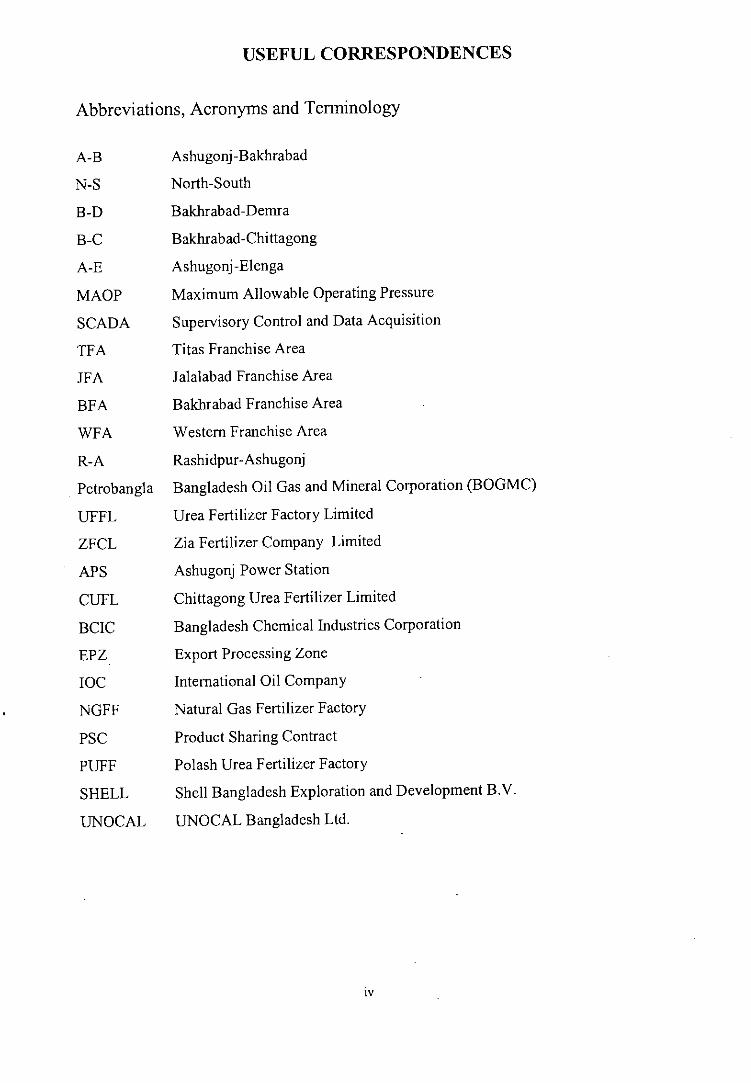
USEFUL CORRESPONDENCES
Abbreviations, Acronyms and Terminology
A-B
N-S
B-D
B-C
A-E
MAOP
SCADA
TFA
JFA
BFA
WFA
R-A
Petrobangla
UFFL
ZFCL
APSCUFL
BCIC
EPZ
IOC
NGFF
PSC
PUFF
SHELL
UNOCAL
Ashugonj-Bakhrabad
North-South
Bakhrabad-Demra
Bakhrabad-Chittagong
Ashugonj-Elenga
Maximum Allowable Operating Pressure
Supervisory Control and Data Acquisition
Titas Franchise Area
Jalalabad Franchise Area
Bakhrabad Franchise Area
Western Franchise Area
Rashidpur-Ashugonj
Bangladesh Oil Gas and Mineral Corporation (BOGMC)
Urea Fertilizer Factory Limited
Zia Fertilizer Company Limited
Ashugonj Power Station
Chittagong Urea Fertilizer Limited
Bangladesh Chemical Industries Corporation
Export Processing Zone
International Oil Company
Natural Gas Fertilizer Factory
Product Sharing Contract
Pol ash Urea Fertilizer Factory
Shell Bangladesh Exploration and Development B.Y.
UNOCAL Bangladesh Ltd.
iv

Operating Companies of Petrobangla
BAPEX
BGFCL
BGSL
GTCL
JGTDSL
RPGCL
SGFL
TGTDCL
Bangladesh Petroleum Exploration Company Limited
Bangladesh Gas Fields Company Limited
Bakhrabad Gas System Limited
Gas Transmission Company Limited
Jalalabad Gas Transmission and Distribution Systems Limited
Rupantarita Prakritik Gas Company Limited
Sylhet Gas Fields Limited
Titas Gas Transmission and Distribution Company Limited
Terminology for metering stations
CGS City Gate station, the pressure is being reduced from the transmission pipelinepressure down to 350/300 psig.
TBS Town Bordering Station reduces pressure from 350/300 psig down to 150 psig.
DRS District Regulating Station reduces pressure from 150 psig down to 50 psig.
Symbols, Measures and Conversion Factors
K
Lac
M
Crore
G
I ton
I barrel (bbl)
I BTU
MCF
TCF
I psig
I atmospheric
= 103
= 105 (Bangladesh Terminology)
= 106 (except for MCF)
= 107 (Bangladesh Terminology)
= 109
= 1000 kg
= 0.159 cubic meter
= 0.252 kilocalorie
= thousand standard cubic feet= Trillion (1,000 billion) cubic feet
= 0.06895 bar
= 14.7 psia
v
(

Chapter
J.
2.
TABLE OF CONTENTS
Abstract
Acknowledge
Useful Correspondences
Table of Contents
List of Tables
List of Figures
List of Appendices
Introduction
Literature Review
2.1 Introduction
2.2 Types of Pipelines
2.2.1 Gas Pipelines
2.2.1.1 Gas Gathering
2.2.1.2 Gas Transportation
2.2.1.3 Distribution Pipeline
2.2.2 Oil Pipelines
2.2.3 Product Pipeline
2.2.4 Two-phase pipeline
2.2.5 LNG Pipelines
2.3 Uses of Natural Gas
2.4 Sector Wise Natural Gas Consumption
2.4.1 Ammonia-Urea Fertilizer Sector
2.4.2 Trends of Natural Gas Uses for Power Generation
2.4.3 Industrial, Domestic and Commercial Sectors
2.5 Gas Sector of Bangladesh
2.5.1 Oil and Gas Exploration in Bangladesh
2.5.2 Gas Fields of Bangladesh
VI
. 'PageNo.HI
III
IV-V
VI-IX
X
XI-Xll1
XIV
1-3
4-34
4
5
5
5
6
6
6
7
7
7
7
8
10
13
17
19
19
22

2.5.3 Present Demand and Supply Scenario 27
2.5.4 Future Demand and Supply Scenario 30
2.6 Gas Transmission Network 32
3. PIPESIM 35-41
3.1 Introduction 35
3.2 PIPESIM-Net 35
3.3 Black Oil and Compositional Data 36
3.4 Calibration Data 37
3.5 Model Overview 38
3.6 Network Validation 39
3.7 Flow Correlations 39
3.7.1 Horizontal Flow 39
3.7.2 Vertical Flow 40
3.7.3 Single Phase Correlations 40
3.8 Convergence 41
4. Gas Transmission System and Related Data 42-51
4.1 Introduction 42
4.2 Network Analysis 42
4.3 Gas Composition 46
4.4 Diameter and Length of Transmission Lines 49
5. Steady- State Flow of Gas through Pipes 52-71
5.1 Introduction 52
5.2 Gas Flow Fundamentals 52
5.3 Types of Single-Phase Flow Regimes and Reynolds Number 53
5.4 Pipe Roughness 54
5.5 Pressure Drop Calculations 555.5.1 The Pressure Drop due to Potentia! Energy Change 555.5.2 The Pressure Drop due to Kinetic Energy Change 555.5.3 The Frictional Pressure Drop 56
vii

5.6
5.7
5.8
Allowable Working Pressures for Pipesr
Allowable Flow Velocity in Pipes
Horizontal Flow
57
57
57
5.8.1 Non- Iteration Equations for Horizontal Gas Flow 58
5.8.2 A More Precise Equation for Horizontal Gas Flow (The 59
Clinedinst Equation)
6.
5.9 Gas Flow through Restrictions
5.10 Sub-Critical Flow
5.11 Critical Flow
5.12 Flowing Temperature in Horizontal Pipelines
5.13 Steady-State Flow in Pipeline Networks
5.13.1 The Mathematical Models for the Individual NCE's
5.13.2 Loop Less System
5.13.3 Looped Systems
5.13.3.1 Single-Loop System
5.13.3.2 Multiple-Loop System
Simulation Results
606061
61
62
63
65
666769
72-115
6.1
6.2
Introduction
Demand-supply Scenario of High-pressure gas transmission lines
72
72
of Bangladesh Using Current Data (from 12-July-00 to 13-July-OO)
6.2.1 North-South Gas Transmission Pipe Line 72
6.2.2 Bakhrabad to Chittagong Gas Transmission Pipe Line 74
6.2.3 Ashugonj to Bakhrabad Gas Transmission Pipe Line 75
6.2.4 Bakhrabad to Demra Gas Transmission Pipe Line 75
6.2.5 Ashugonj to Elenga Gas Transmission Pipe Line 75
6.2.6 Titas - Narshingdi - Demra Gas Transmission Pipe Line 76
6.2.7 Titas - Narshingdi - Joydevpur Gas Transmission Pipe 76
Line
6.2.8 Monohordi - Narsingdi - Shiddirgonj Gas Transmission 77
Pipe Line
6.2.9 Western Region Gas Transmission Pipe Line 77
viii

6.3
6.4
6.5
6.6
6.7
6.8
6.2.10 Network Analysis
Modification of Network by Using Known Pressure at Bakhrabad
Gas Field
Modification of Network by Setting up a Compressor Station at
Bakhrabad Gas Field
Gas Demand-Supply Scenario of High Pressure Transmission Line
at Maximum Load
Modified Network Using R-A Loop Line
Extension of Network up to Bheramara
Extension of Network up to Khulna without Modification
6.8.1 Extension of Network up to Khulna with A-D Loop Line
6.8.2 Modification ofNolka to Khulna line by Using Loop Line
from R-A Loop Line to Dhanua
6.8.3 Modified Final Network by Using Compressor Station at
Monohordi
77
85
90
93
96
101
104
107
110
113
References
Nomenclature
Discussions
Conclusions and Recommendations
116-118
119-120
119
120
121-143
144-145
146-147
Conclusions
Recommendations
Appendices
8.1
8.2
7.
8.
ix

LIST OF TABLES
31
334748
49
29
29
28
. Page'No'.
9
13
16
2021
24
25
28
Sector Wise Natural Gas Consumption
Connected Maximum Loads of Gas for Fertilizer Sectors
Trends of Natural Gas Uses for Power Generation
Exploration Phases of Bangladesh
Exploration Activities in Bangladesh since 1972
Gas Fields of Bangladesh
Production Capacities of Various Gas Fields
Downstream Demand and Consumption of Natural Gas of Jalalabad
Gas Franchise Area (JFA), Greater Sylhet
Downstream Demand and Consumption of Natural Gas of Titas
Gas Franchise Area (TFA)
Downstream Demand and Consumption of Natural Gas of
Bakhrabad Franchise Area (BFA)
Downstream Demand and Consumption of Natural Gas of Western
Region Franchise Area (WFA)
Average Base Case SupplylDemand (in MMCFD)
Gas Transmission Network
Gas Composition of Natural Gas in Different Gas Fields
Sales Gas Specification ofTitas Franchise Area
Length and Diameter of Major Gas Transmission Pipelines of
Jalalabad Franchise Area
Table 4.4 Length and Diameter of Major Gas Transmission Pipelines of Titas 50
Franchise Area
Table 2.12
Table 2.13
Table 4.1
Table 4.2
Table 4.3
Table 2.11
Table 2.10
Table 2.9
Table 2.1
Table 2.2
Table 2.3
Table 2.4
Table 2.5
Table 2.6
Table 2.7
Table 2.8
Table 4.5 Length and Diameter of Major Gas Transmission Pipelines of 50
Bakharabad Franchise Area
Table 4.6 Length and Diameter of Major Gas Transmission Pipelines of 51
Western Region Franchise Area
Table 6.1 Comparison of Simulated Pressure to the Measured Pressure 83
x
Page No ..10II
121417233843
III 45
Figure 2.1
Figure 2.2
Figure 2.3
Figure 2.4
Figure 2.6
Figure 2.5
Figure 3.1
Figure 4.1
Figure 4.2
Figure 4.3
Figure 5.1
Figure 5.2
Figure 5.3
Figure 5.4
Figure 6.1
Figure 6.2
Figure 6.3
Figure 6.4
Figure 6.5
Figure 6.6
Figure 6.7
Figure 6.8
Figure 6.9
LIST OF FIGURES
Sector Wise Natural Gas Consumption
Natural Gas Consumption in Bangladesh
Urea Plants in of Fertilizer Factories of Bangladesh
Power Plants in Bangladesh
Trends of Natural Gas Uses for Power Generation
Natural Gas Fields in Bangladesh
Types of Network Used in PIPESIM-Net
The Geographical Areas for the Gas System Development Plan
Gas Transmission Network, Main High Pressure Lines
Bangladesh
Gas Transmission Network, Possible Extension m the Western
Region
Loop Less Pipeline System
Single Looped Systems
Multiple Looped System
Illustration for Stoner's Method
High Pressure Gas Transmission Lines of Bangladesh Using
Current Data
Variation of Pressure along the Major Gas Transmission Lines
Change of Flowrate along the Major Gas Transmission Lines
Change of Liquid Hold up along the North-South line
Demand-Supply Scenario of High-pressure Gas Transmission
Lines of Bangladesh Modified by Known Pressure at Ashugonj
Calculated and Measured Pressure along the N-S Line
Variation of Pressure along the Major Gas Transmission Lines
after Modification
Variation of Pressure along the Major Gas Transmission Lines
Demand-Supply Scenario of High-pressure Gas Transmission
Lines Modified by Using Known Pressure at Bakhrabad Gas Field
xi
46
65
67676973
7878
8081
8282
84
87
Figure 6.10
Figure 6.11
Figure 6.12
Figure 6.13
Figure 6.14
Figure 6.15
Figure 6.16
Figure 6.17
Figure 6.18
Figure 6.19
Figure 6.20
Figure 6.21
Figure 6.22
Figure 6.23
Figure 6.24
Variation of Pressure along Major Transmission Lines Modified
by Using Known Pressure at Bakhrabad Gas Field
Variation of Flow Rate along Major Transmission Lines Modified
by Using Known Pressure at Bakhrabad Gas Field
Effect of Separator on North-South Line
Demand-Supply Scenario of High Pressure Gas Transmission
Lines Modified by Setting up a Compressor Station at Bakhrabad
Gas FieldVariation of Pressure along Major Gas Transmission Lines by
Dropping Bakhrabad Gas Field from the Network
Change of Flow Rate along Major Gas Transmission Lines by
Dropping Bakhrabad Gas Field from the Network.
Effect of Compressor at Bakhrabad Gas Field
Gas Demand-Supply Scenario of High Pressure Transmission Line
at Maximum Load
The Variations of Pressure along the Major Transmission Lines
Modified by Maximum Load
Change of Flow Rate along the Major Transmission Lines
Modified by Maximum Load
Demand-Supply Scenario of High Pressure Gas Transmission
Lines Modified Network by Using R-A Loop Line
The Variations of Pressure with the Length after Modified by R-A
Loop LineChange of Flow Rate with the Length after Modified by R-A Loop
LineDemand-Supply Scenario of Gas Transmission Lines Modified by
Using R-A Loop Line and Mentioning Known Pressure at
AshugonjThe Variations of Pressure with the Length after Modified by R-A
Loop Line for Pressure Matching
xii
88
88
8991
92
92
93
94
95
95
98
99
99
100
101
Figure 6.25 Demand-Supply Scenario of High Pressure Gas Transmission 102
Lines by Extension of Network up to Bheramara
Figure 6.26 Variation of Pressure Drop along Major Transmission Lines by 103
Extension of Network up to Bheramara
Figure 6.27 Change of Flow Rate along the Major Transmission Lines by 103
Extension of Network up to Bheramara
Figure 6.28 Demand-Supply Scenario of High-pressure Gas Transmission 105
Lines by Extension of Network up to Khulna without Modification
Figure 6.29 The Variation Pressure of Major Transmission Lines by Extension 106
of Network without any Modification
Figure 6.30 Change of Flow Rate along the Major Transmission Lines by 106
Extension of Network without any Modification
Figure 6.31 Demand-Supply Scenario of High Pressure Gas Transmission 108
Lines by Extension of Network up to Khulna with A-D Loop Line
Figure 6.32 The Variation of Pressure along the Major Transmission Lines by 109
Extension of Network up to Khulna with A-D Loop Line.
Figure 6.33 Change of Flow Rate along the Major Transmission Lines by 109
Extension of Network up to Khulna with A-D Line
Figure 6.34 Demand-Supply Scenario of High Pressure Gas Transmission III
Lines modified by Using Loop Line from R-A Loop Line to
Dhanua
Figure 6.35. The Pressure Drops of Major Transmission Lines of Nolka to 112
Khulna Pipeline Using Loop Line from R-A Loop Line to Dhanua
Figure 6.36 Change of Flow Rate along the Major Transmission Lines of 112
Nolka to Khulna Pipeline Using Loop Line from R-A Loop Line
to Dhanua
Figure 6.37 Demand-Supply Scenario of High Pressure Gas Transmission 114
Lines modified Final Network by Using Compressor Station at
Monohordi
Figure 6.38 The Variation of Pressure along the Major Transmission Lines lIS
modified by Using Compressor Station at Monohordi
Xlll

LIST OF APPENDICES
-1IP .. :" -~---_.,_ .. _~-<>---. ----. -~--~--~--- ,"
Appendix I
Appendix 2
Appendix 3
Appendix 4
Appendix 5
Appendix 6
Simulated Results of High Pressure Gas Transmission Lines of
BangladeshSimulated Results of High Pressure Gas Transmission Lines of
Bangladesh modified by Known Pressure at Ashugonj
Simulated Results of High Pressure Transmission Lines Using
Known Pressure at Bakhrabad Gas Field.
Simulated Results of High Pressure Transmission Lines by
Setting up a Compressor Station at Bakhrabad Gas Field
Simulated Results of High Pressure Transmission Lines at
Maximum Load.
Simulated Results of High Pressure Transmission Lines
Modified Network Using R-A Loop Line.
121
123
125
127
129
130
Appendix 7 Simulated Results of High Pressure Transmission Lines 132
Modified Network Using R-A Loop Line by Using Known
Pressure at Ashugonj.
Appendix 8 Simulated Results of High Pressure Transmission Lines 135
Modified Network by Extension of Network up to Bheramara.
Appendix 9 Simulated Results of High Pressure Transmission Lines 137
Extension of Network up to Khulna without any Modification
Appendix 10 Simulated Results of High Pressure Transmission Lines 138
Extension of Network up to Khulna with A-D Loop Line.
Appendix II Simulated Results of High Pressure Transmission Lines, 140
Modification of Nolka to Khulna Line by Using Loop Line
from R-A Loop Line to Dhanua
Appendix 12 Simulated Results of High Pressure Transmission Lines 143
~ Modified Network by Using Compressor Station at Monohordi
xiv

Chapter 1
INTRODUCTION
The importance of mineral and energy resources cannot be over emphasized in a
developing country like Bangladesh. These resources are not only considered as the driving
" force but also the backbone of modem economy. These are vital requirement for
industrialization, power generation etc. and thus for enhancement of the social standards of
people through economic development and attainment of comfortable life style. In this
context it is important that the government should make sincere efforts for the development
of this sector.
:':"-
Natural gas is the most important non-renewable resources in Bangladesh. Over the years it
has acquired a position as.an alternative to oil. It is also regarded, as a main source of power
generation. Its use and requirement has been greatly enhanced in recent times. During the
pre-liberation period, around 1968-69, the use of gas stood at 19 percent of total
commercial energy only, when the consumption of oil was more than 70 percent. From 80's
the consumption of natural gas rose a little above 37 percent, and by 90's the consumption
of gas exceeded 70 percent and simultaneously it distinct decrease was noticed in the
consumption of oil and it came down to 30 percent.
Bangladesh has discovered 22 gas fields and one oil well (Sylhet 7 at Haripur). But 12
producing gas fields can produce 1300 MMCFD of gas from 53 gas wells. In 22 gas fields,
total GIIP (proven + probable) reserve is about 24.745 TCF of which about 15.507 TCF (1)
has been confirmed. Out of recoverable reserve, 4.08 TCF gas has been consumed (I). The
present peak demand of 1089 MMCFD (2) which can now be met from the current peak
production of 1300 MMCFD after drawing gas from private producers, namely, UNOCAL
il., Bangladesh Ltd. and Shell Bangladesh Exploration and development B.V. Of the total gas
produced, 35 percent is used for fertilizer, 45 percent for power generation and 20 percent
for other purpose (I).

1.J; 2.
3.
4.
The gas transmission pipelines In Bangladesh were initially planned and constructed
targeting particular bulk consumers or potential load centers. In the early stage of the
development of the gas sector, the grid system was not visualized. But over the years the
gas transmission system has expanded considerably and has become complicated. Four
Companies of Petrobangla'such as Gas Transmission Company Ltd. (GTCL), Titas Gas
Transmission and Distribution Company Ltd. (TGTDCL), Bakhrabad Gas Systems Ltd.
(BGSL), Ialalabad Gas Transmission and Distribution Company Ltd. (IGTDCL) and two
international companies (Unocal Bangladesh Ltd., Shell' Bangladesh Exploration and
Development B.V.) are responsible for operation and maintenance of their respective
transmission pipelines.
As new gas based industries and power plants are being set up, the existing gas
transmission system is being stressed to meet the demand. To overcome this, a loop line is
being constructed from Kailashtilla to Ashuganj to flow more gas from Sylhet region. To
study the performance and the effect of any future development, it is required to analyze the
whole transmission network.
The objective of this study is to perform gas transmission network analysis of Bangladesh.
Various components of the objective are:
i) to simulate the present gas transmission net~ork system and compare with the
actual performance
ii) to identify any limitation of the system
iii) to study the effect of future pipeline expansion, loads etc.
This study has been carried out using a software called PIPESIM. Baker I ardine Inc. (UK)
developed it. Building the pipeline network using the software can be divided in to a
number of stages:
Collecting all necessary data on the transmission network
Setting up the model and naming components
Setting global default (fluid composition, unit etc.)
Setting boundary conditions at wells, sources and sinks (loads)
2

5. Running the model and analyzing the results
The study has been undertaken to simulate the present network system, identify its
limitations and suggest remedial measures. This study would be useful to understand the
performance of the present gas transmission system of Bangladesh. This study would also
analyze the existing pipeline capacity and examines the level of capacity utilization. The
simulated results will be helpful to identify the bottlenecks and to plan for future expansion.~
of gas transmission system.
(
'-
3
"

!
Chapter 2
LITERATURE REVIEW
2.1 Introduction
The natural gas has established itself as a major indigenous hydrocarbon resource in
Bangladesh. It is the chief source of fuel for industrial, commercial and household
operations as well as for power generation. On September 18, 2001 the production was
1042 MMSCFD and the two laCs' contribution was 176 MMSCFD (1) The present peak
demand is about 1089 MMSCFD.
The first discovery of natural gas was made in 1955 at Haripur. Since then the exploration
has led to the discovery of 22 gas fields and one oil field. There are now 53 producing wells
capable of producing about 1300 MMSCFD of gas from 12 gas fields (1) The exploration
activities for gas and oil in Bangladesh started with the exploration at Sitakunda in 1908.
National Energy Policy (NEP), promulgated in 1995, indicated an energy-growth rate of
8.77% by year 2000 equivalent to 12 million tons of oil and 19 million tons of oil
equivalents, representing energy growth rate of 8.86% (3). The major part of the future
energy demand would be met from natural gas and it is estimated that gas demand would
reach about 1450 MMSCD (average) and 1700 MMSCFD (maximum) by 2005 and 1900
MMSCFD (avg.) and 2250 MMSCFD (4) by 2010 (max.) ..
The uses of Natural gas in Bangladesh can be broadly classified into five categories,
namely, power, fertilizer, industrial, commercial and domestic. The fertilizer sector utilizes
natural gas as a feed stock as well as fuel while the remaining sectors use it as a fuel. The
current consumption pattern shows that fertilizer sector consumes approximately 35%,
power 45% and other sectors (industry, domestic, commercial arid seasonal) 20% of the
gaseS). \,
4
2.2 Types of Pipelines
A network of sophisticated pipeline systems transports oil, natural gas and petroleum
products from producing fields and refineries around the world to consumers in every
nation. This network gathers oil and gas from hundreds of thousands of individual wells,
including those in some of the world's most remote and hostile areas. It distributes a range
of products to individuals, residences, businesses and plants.
Most gas and oil pipelines fall into one of three groups: gathering, transportation or
distribution (6) Other pipelines are needed in producing fields to inject gas, water or other
fluids into the formation to improve gas and oil recovery and to dispose of salt water often
produced with oil.
2.2.1 Gas Pipelines
In general, gas pipelines operate at higher pressure than crude lines; gas is moved through a
gas pipelines by compressor rather than by pumps; and the path of natural gas to the user is
more direct.
2.2.I.I Gas Gathering
Gas well flow lines connect individual gas wells to field gas treating and processmg
facilities or to branches of a large gathering system. Most gas wells flow naturally with
sufficient pressure to supply the energy needed to force the gas through the gathering lines
to the processing plant. Down hole pumps are not used in gas wells, but in some very low
pressure gas wells, small compressors may be located near the well head to boost the
pressure in the line to a level sufficient to move the gas to the process plant.
5 r'I\ \'_ ..

2.2.1.2 Gas Transportation
From field processing facilities, dry, clean natural gas enters the gas transmission line
system for movement to cities where it is distributed to individual business, factories and
residences. Distribution to the final users is handled by utilities that take custody of the gas
from the gas transmission. pipeline and distribute it through small, metered pipelines to
individual customers.
Gas transmission lines at relatively high pressures. Compressors at the beginning of the line
provide the energy to move the gas through the pipeline. Then compressor stations are
required at a number of points along the line to maintain the required pressure. The distance
between the compressors varies, depending on the volume of gas, the line size and other
factors. Adding compressors at one or more of these compressor stations or by building an
additional compressor station often increases capacity of the system. The size of the
compressors with in the station varies over a wide range, but many stations include several
thousand horsepower in one station.
2.2.1.3 Distribution Pipeline
Through distribution networks of small pipelines and metering facilities, utilities distrjbute
natural gas to commercial, residential and industrial users.
2.2.2 Oil Pipelines
Flow lines, the first link in the transportation chain from producing well to consumer, are
used to move produced-oil from individual wells to a central point in the field for treating
and storage.
6
•

2.2.3 Product Pipeline
The industry's products pipeline system is a sophisticated network. Many segments of the
system are highly flexible in both capacity and the products that can be transported. One
part of this system moves refined petroleum products from refineries to storage and
distribution terminals in consuming areas. Another group of product pipelines is used to
transport liquefied petroleum gases (LPG) and natural gas liquid (NGL) from oil and gas
processing plants to refineries and petrochemical plants.
2.2.4 Two-phase Pipeline
In most cases, it is desirable to transport petroleum as either a gas or a liquid in a pipeline.
In a line design to carry a liquid, the presence of gas can reduce flow and pumping
efficiency; in a gas pipeline, the presence of liquids can reduced flow efficiency and
damage gas compressors and other equipment.
2.2.5 LNG Pipelines
Liquefied natural gas (LNG) is natural gas cooled and compressed to a temperature and
pressure at which it exits as a liquid. Significant volumes of natural gas are transported in
the liquid phase as LNG, but these shipments are made by special ocean tanker rather than
by long distance pipeline.
2.3 Uses of Natural Gas
The uses of natural gas in Bangladesh can be broadly classified into the following five
categories:
Fertilizer: As raw material for production of Urea Fertilizer.
Power: As fuel for generation of electricity.
Industrial: As fuel for various industries.
Commercial and
7
(I\

oj)
".
Domestic.
The current consumption pattern shows that fertilizer (ammonia-urea) sector consumes
approximately 35%, power 45% and other sectors (industry, domestic, commercial and
seasonal) 20% of the gas (5).
2.4 Sector Wise Natural Gas Consumption
During the international energy crisis of the 1970's, the rapid rise in international oil prices
increased the demand for natural gas in different sectors for its lower cost. A more
attractive incentive to use natural gas is its easy and clean burning with environment
benefits. With the growth of the economy, demand for energy has increased.
From Table 2.1 and Figure 2.1 show that natural gas consumption In the power and
fertilizer sector started increasing drastically in the mid-80s. This is because at that time
most of the power plants in the eastern grid was being converted from diesel to natural gas
and at the same time some new power plants based on gas were added to the national grid.
In the fertilizer sector, three big urea plants were installed from the middle of 80s to the
beginning of 90s. Industrial and commercial demands also increased during that period,
although the overall percentages or these two sectors were not as significant as the other
two.
In 1996-97, consumption of natural gas in fertilizer sector decreased due to supply crisis of
natural gas in the Chittagong region. As a result, Chittagong Urea Fertilizer factory (CUFL)
stopped its production. Power sector was given priority for supplying gas at that time. After
completion of Ashuganj-Bakhrabad pipeline (A-B pipeline) and production of gas from
Sangu and Jalalabad gas field by two IOCs, CUFL again started production and natural gas
consumption in fertilizer sector increased. A similar supply shortage also occurred during
1989-91 'period due to a fatal accident at Ghorasal Fertilizer Factory. Presently there is no
shortage of supply and daily demand is about 930 MMSCFD.
8

>
,'.-
Table 2.1 : Sector Wise Natural Gas Consumption (8)
Year .•.~~"' '.- - ,~ .,. I- .,"'" ~:; - "'Sectors (MMSCF):-', ~'_". ~~~I.~-r "':~~-":=!'I')";',-~~..:~~'- .,
Power Fertilizer Industrial Commercial. Domestics • Total
1967-68 225 0 0 0 0 225
1968-69 1019 0 5 9 I 1034
1969-70 1140 1828 145 26 4 3143
1970-71 3419 4225 255 41 22 7962
1971-72 3103 602 322 33 36 4096
1972-73 4513 9669 843 66 87 15178
1973-74 7419 10559 1462 115 146 19701
1974-75 6063 2098 1784 181 277 10403
1975-76 6535 11018 2334 266 489 20642
1976-77 8200 10027 3047 370 766 22410
1977-78 9327 8311 3742.17 571.27 1125.43 23076.87
1978-79 9209 11146 4557.36 854.55 1873.09 27640
1979-80 11018 11975 5182.99 1078.10 2561.84 31815.93
1980-81 13321 11210 5978.60 1342.47 3390.00 35242.07
1981-82 18010 19836 7391.06 1680.98 4214.25 51132.29
1982-83 21999 19140 7812.44 1917.57 5217.24 56086.25
1983-84 22886 25805 8687.83 2057.67 5785.14 65221.64
1984-85 38292.70 24296 11447.76 2232.62 6318.95 82588.03
1985-86 39778.27 30070.50 16352.56 2721.54 6796.95 95719.82
1986-87 51852.09 33474.5 18673.16 3415.81 6840.79 114256.35
1987-88 63054.45 50978.72 15665.47 3603.63 7590.41 140892.68
1988-89 66455.80 57886.51 1497.08 3126.15 9261.28 151026.82
1989-90 75557.45 55909.11 13892.44 3098.67 10418.70 158876.37
1990-91 82556.11 54172.33 13911.78 2930.55 10529.37 164100.14
1991-92 88105.07 61642.31 14088.55 3135.73 11645.93 178617.59
1992-93 93212.08 69176.18 15801.05 2547.99 13495.68 194232.98
1993-94 97491.11 74434.89 19895.15 2853.89 15603.05 210278.09
1994-95 107437.37 80464.44 23891.25 2896.42 18781.78 233471.26
1995-96 110827.15 90979.45 27189.53 3029.01 20776.44 252801.58
1996-97 110864.20 77828.57 29303_97 3393.48 22869.06 244259.28
1997-98 123391.93 80000.68 33046.61 3496.83 24984.67 264920.72
1998-99 140837 82730 35779 3652 27183 290181
1999-00 149355 84894 41271 3836 29675 3090312000-01 175204 88465 48094 4066 31872 347701
Total 1761678 1254852 433349.8 64645.93 300638.1 3827964
9
.'..\!!~..(.• .•.... ~•• •

IndustrialCommercial .
--lIE- Domestic
_.~~------
400000 -+- Power
~ 350000-11- Fertilizeru2 300000
::8 250000
.~ 200000a- 150000 __ Total;:l
:g 100000-ou 50000.' -~-~----~~-~~~~~~~o - - w -T-'~'--'-T-'-'-'-'-r-' I
. _.__ __.~96: __._1_97_0 1_975 1~8_0__Year_1985 .~_90__ 1~~___ 2~~~_J
In 1968-69, out of a total consumption of 1034 MMSCF, power sectors alone used 98% of
the total gas and commercial, industrial and domestic sectors together used only 2%. With
the introduction of gas in the Urea Fertilizer Factory Limited (UFFL) at Ghorasal in 1970,
the total demand for gas stood at 7962 MMSCF. Percentage use of gas in power, fertilizer,
industrial and commercial sectors was43%, 53%,4% and 0.5% respectively. Domestic use
of gas was 3% in 1970-71, which increased to 8% in 1979-80. Use of gas in power sector
kept on increasing and in 1996-97 its share was 46%. Figure 2.1 shows percentage of gas
consumption in different sectors from the beginning of its use. It is anticipated that more
and more gas would be used to meet the power demand of the country.
Figure 2.1: Sector Wise Natural Gas Consumption (8)
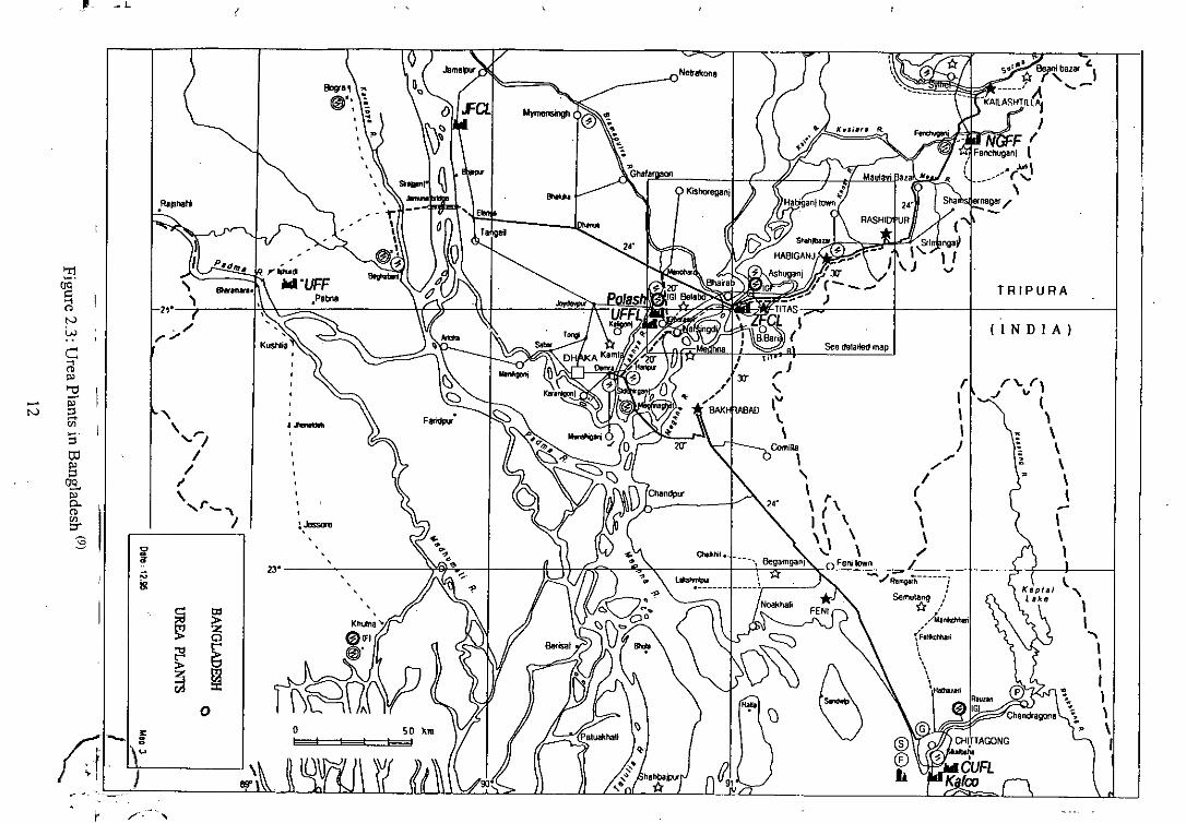
2.4.1 Ammonia-Urea Fertilizer Sector
Seven ammonia-urea complexes now in operation have a combined connected demand of
289 MMSCFD of gas (5). Table 2.2 shows the growth of this sector, and Figure 2.2 shows
the consumption trend of gas since 1960 with the commissioning of each plant. During the
decade of 1988-1997 the share of this sector accounted for 32 to 37 % of the total gas
consumed (5). The locations of fertilizer factories are shown in Figure 2.3.(
10

. 2008
.2007200620052004200320022001200019991998
. 19971996 ~1995 ~1994 0-1993 u
~~ .
"" .
1992 VJ
"'!" ::; ••• 1
~'.
1991 "N u ' .~N u.. : 1990, is
~ 1989 .;::~-' 1988 "LL
u-ri r:: ::> 1987 .S
u@j~.<t 1986 "co LL I~::> '. 1985 0
a. '.;::
, 1984 0-
1983 ~ E0 '"~. 1982 0> ::l ->- <n
d ..••--- 1981 "0LL 1980 UN 1979 <n
'"1978 01977 :a
0 1976 ~::l
I LL . 1975 -u '"
I(J)
1974 Z:;:; 1973 "!
i 2. ~rI1972 N
.-: <o;J c: .••• 1971 "
u~
ro 1970 ::l
0! lD ~ ,~
...J1969 u-
Vl. 1968
ro(9
1967(\)
. 1966.20 1965iii'S . in
1964
'" E 1963~ "
::. 1962u LL
t ro LL •• . 1961'" (5 0
0
u. f-z 1960,
t T195919581957
0 '" 0 0 0 0 0 0
0 '" 0 0 0 0 0
0""
0 0 0 0 0 (0 r, 0 0 0 0 0
'" 6 '" 0 '" 0 '"co co N N ~ ~ \(:l::JSIJIJiI\I)UO!ldlUnsuo::J se~
, ,,, .
"~" _ LI
~'\,,..,III1,. \
II
TRIPURA
r'\. r,J " (,
\\\\\-I
\,
(INDIA)
v
r,\\
J;-
'"I(,\\
'"
See delailed map
Comi'Aa,",\ '\I ( ,,\ ,
\,., \Felli lown---;;;:;;'/Relll~-----7
Semula~ /
* "/Manldrlle'il
{;.1k:hhIri
\.\
'.HlIltIIlarl
l,Jessore
••••••••••
23'
Io
'I,A
",
~
~
"',-,')I/
"\,r~,I
".,.,;,'"
~ill
Ii
/"f-h! IJ:.[ )~- .
"r1~.~"Nw
C~"'""C- ~N ~'"5"togj03-'"p.."'"::r':s
I'" /,

Table 2.2: Connected Maximum Loads of Gas for Fertilizer Sectors (5)
From Year Plant " ' Load(MMSCFD) ,.' Cumull:1tiv~(MMSCFD)1961 NGFF 19 191970 UFFL 45 641981 ZFCL 50 1141986 PUFF 17 1311987 CUFL 50 1811991 JFCL 43 2241994 KAFCO 65 289
During the period 1986 to 1987, a gas load of 67 MMSCFD was added by the fertilizer
sector with the commissioning of PUFF and CUFL while an additional load of 108
MMSCFD was added during 1991-94 when JFCL and KAFCO came on stream. The
average daily demand of gas by the fertilizer sector for the years 1986, 1989 and 1996 were
103, 154 and 213 MMSCFD respectively against the contracted loads of 121,171 and 284
MMSCFD respectively. During the next five years, the most optimistic annual consumption
of gas would be 90,000 MMSCFD by this sector.
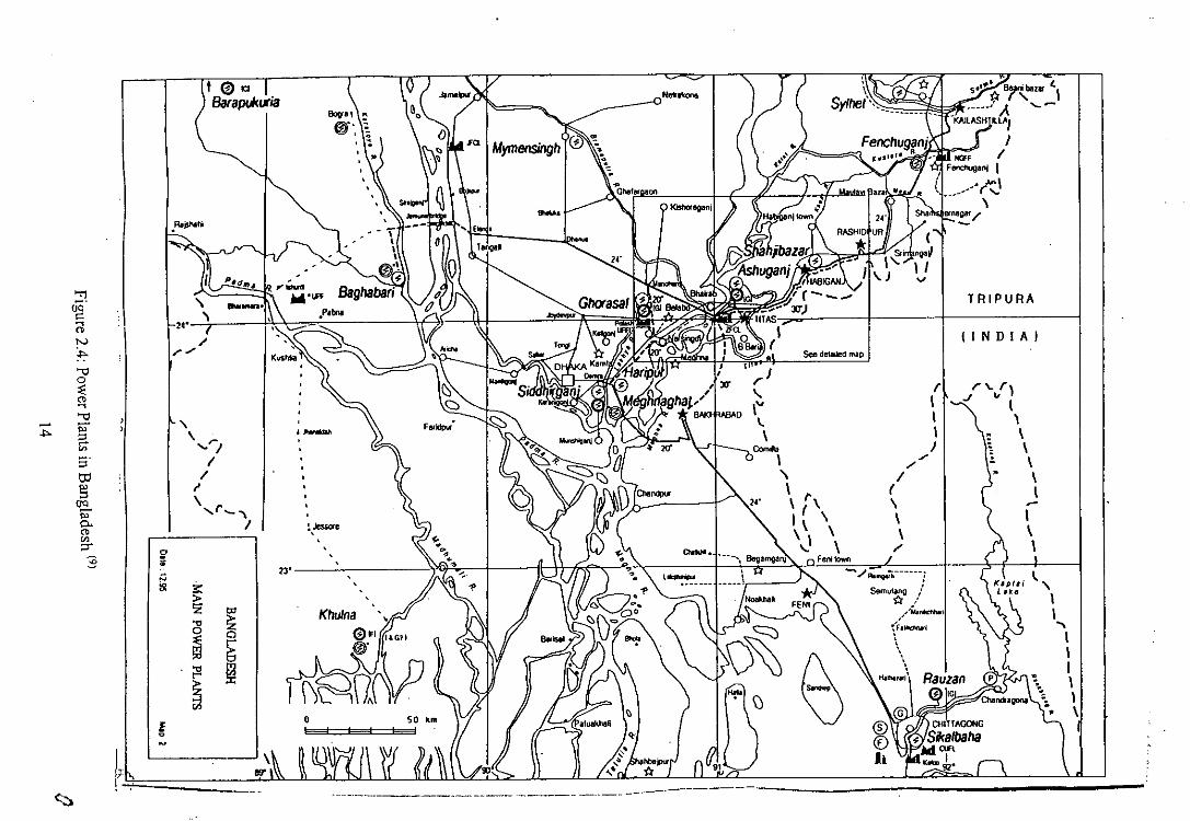
2.4,2 Trends of Natural Gas Uses for Power Generation
From the present trend of economic growth in different areas it is clear that most of the
future gas demand would come from the power sector. A more detailed and lists of the gas
demand scenario in power sector enable us to have a better understanding of the growth
projection. The location of gas based power stations of Bangladesh are shown in Figure 2.4.
Natural gas was first introduced on a trial basis for power generation in Bangladesh in 1967
in a 30 MW power plant at Siddirgonj. Use of gas to produce electricity increased steadily
and in 1999 installed generating capacity by using natural gas stood at 2575 MW which is
about 75% of the total installed capacity. In December 1999, natural gas was supplied to the
western zone for the first time and it is expected that several gas-fired power plants would
be established in the power starved western zone of the country.
13
--------------------------- ------------------------------------
v
See de1ailed map
'-,\I"'I,I\\\
TRIPURA
r \. r\J ~
I,I,\\I-I,\
(I N D I A I
rII\
J.r
./I{\,,./
-./R.~---~--!Semutang ••~ ,.
~-M.~;I,-\FIl'r;H\¥i
\.\
IiIll>lIl.1
rJ\.\"'-I
Com"\
"\, '\I '
"\..'
~
~~Jessorll
.-Kushlla
I-.A.
"2~.~/
/.;/
<;)
>r1QQ''"...,'"tv~-00~'"...,-0- '"..,. ::lfA:;OJ~<e.~'"en;:r3

Table 2.3 shows that natural gas consumption started increasing in power generation from
the very beginning after the installation of a 30 MW trial plant in 1967. Conversion of the
old oil-fired plants and addition of some new power plants pushed the total demand of gas
to the present value. From Figure 2.5 it is clear that in mid 80's, natural gas used power
generation increased sharply. This was due to the addition of three 210 MW units at
Ghorasal and three 150 MW units at Ashuganj. In mid 90's another new power plant at
Raozan with two units each of 210 MW capacity was added to the national grid. A sharp
rise in natural gas consumption curve can be observed during that period. Furnace oil and
HSD/SKO consumed in power generation, mainly in the remote areas and western zone
where natural gas is not available remains almost same from the beginning. Natural gas
completely replaced the use of naphtha and coal in power generation in 1972 and 1983
respectively.
15
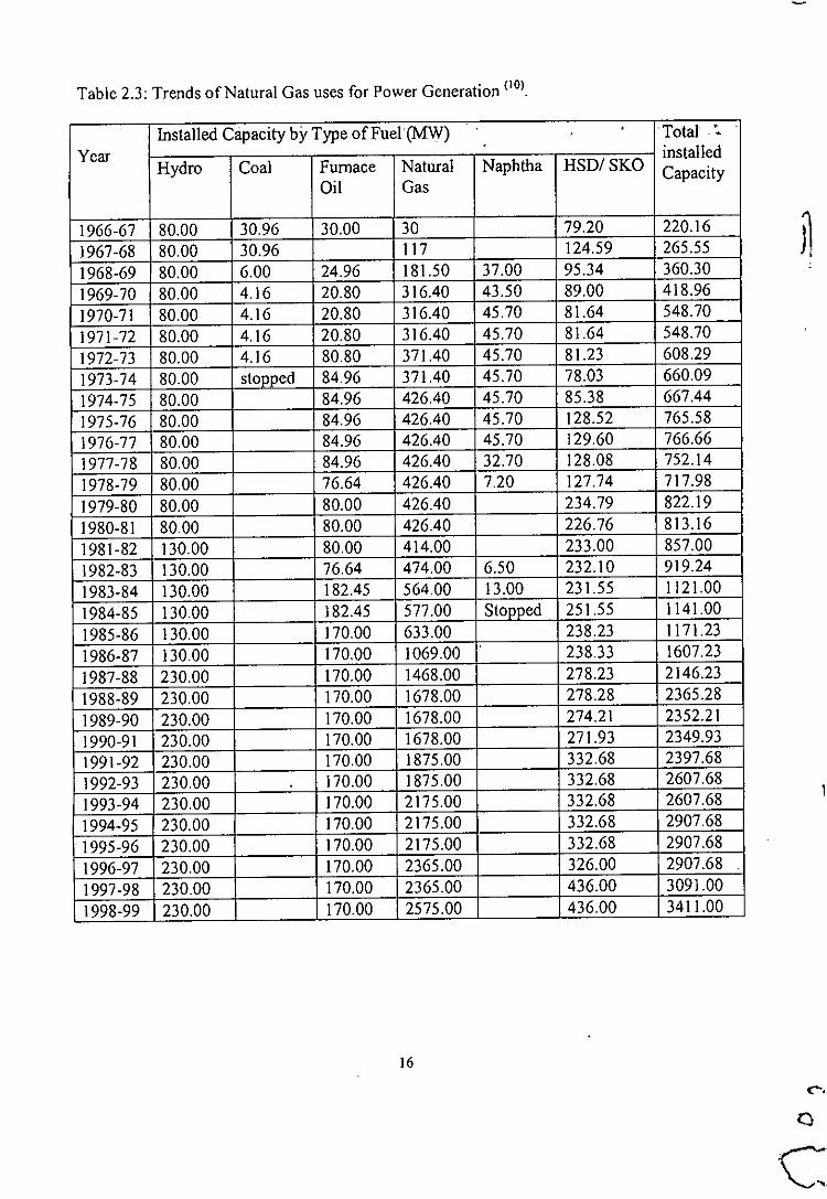
Table 2.3: Trends of Natural Gas uses for Power Generation (10).
Installed Capacity by Type ofFuel(MW) . Total "Year
Hydro Coal Furnace Natural Naphtha HSD/SKOinstalledCapacity
Oil Gas
1966-67 80.00 30.96 30.00 30 79.20 220.161967-68 80.00 30.96 117 124.59 265.551968-69 80.00 6.00 24.96 181.50 37.00 95.34 360.301969-70 80.00 4.16 20.80 316.40 43.50 89.00 418.961970-71 80.00 4.16 20.80 316.40 45.70 81.64 548.701971-72 80.00 4.16 20.80 316.40 45.70 81.64 548.701972-73 80.00 4.16 80.80 371.40 45.70 81.23 608.291973-74 80.00 stoDDed 84.96 371.40 45.70 78.03 660.091974-75 80.00 84.96 426.40 45.70 85.38 667.441975-76 80.00 84.96 426.40 45.70 128.52 765.581976-77 80.00 84.96 426.40 45.70 129.60 766.661977-78 80.00 84.96 426.40 32.70 128.08 752.141978-79 80.00 76.64 426.40 7.20 127.74 717.981979-80 80.00 80.00 426.40 234.79 822.191980-81 80.00 80.00 426.40 226.76 813.161981-82 130.00 80.00 414.00 233.00 857.001982-83 130.00 76.64 474.00 6.50 232.10 919.241983-84 130.00 182.45 564.00 13.00 231.55 1121.001984-85 130.00 182.45 577.00 StoDDed 251.55 1141.001985-86 130.00 170.00 633.00 238.23 1171.231986-87 130.00 170.00 1069.00 238.33 1607.231987-88 230.00 170.00 1468.00 278.23 2146.231988-89 230.00 170.00 1678.00 278.28 2365.281989-90 230.00 170.00 1678.00 274.21 2352.211990-91 230.00 170.00 1678.00 271.93 2349.931991-92 230.00 170.00 1875.00 332.68 2397.681992-93 230.00 170.00 1875.00 332.68 2607.681993-94 230.00 170.00 2175.00 332.68 2607.681994-95 230.00 170.00 2175.00 332.68 2907.681995-96 230.00 170.00 2175.00 332.68 2907.681996-97 230.00 170.00 2365.00 326.00 2907.681997-98 230.00 170.00 2365.00 436.00 3091.001998-99 230.00 170.00 2575.00 436.00 3411.00
16
'c

1--
'Q)
.2'+- 4000 -~-----_.- --:.. -o __ Hydro-all~ 3500 - __ Coal
~ 3000 Furnace oil£; 2500 Natural gas>-~
.0 S 2000 __ Naphtha>-:2'5 ~1500 - -- HSD/SKOrog- 1000'-::+- ~?ta~ _u"0 500Q)
,ro 0I~I ~ 1960 1970
1\ ' -- -'~.•.•.~'-,--.---.:1::
1980
Year
1990 2000
---_.-----_._--- --- ------ ------_.- -----_._._---------------_.----~----_. __ .-
Figure 2.5: Trends of Natural Gas uses for Power Generation (10)
2.4.3 Industrial, Domestic and Commercial Sectors
In the current decade, percentage of total gas consumed by the combined industry, domestic
and commercial sector uses between 16 and 22. Commercial consumers account for less
than 1.5% of the total gas consumption and the sector has not shown significant growth
during the past decade.
Industry, the main contributor among others has reached again the 1986-87 level after years
of substantial decline. This fall is partly related- to the poor growth performance of the
manufacturing sector in Bangladesh, only 3.1% as yearly growth for the period 1980-92.
During the same period the whole industry had better performances since the growth rate
has reached 5.1% a year for the period 1990-92 according to World Bank statistics. The
industrial sector during the current decade has been using 8 to 12% of the total gas
consumption. Major application areas in this sector include steam generation, captive power
17
r;:.1 '.

and for process (heating media and heat source). When the Bakhrabad Gas Systems Ltd.
had made natural gas available in Chittagong area, industries using furnace oil, disel or
other liquid fuels immediately switched over to gas. These include ERL, TSP, KPM, KRC,
Osmania Glass, Chittagong Steel Mills, etc. For the industry sector, the growth has been
3.75% during the decade 1986-1995.
In Bangladesh, the domestic sector has ex'perienced a steady growth since the beginning.
Within the Titas Franchise area the average growth has reached 9.7% a year from 1980-81
to 1993-94. For Bakhrabad Franchise area development of gas sales to domestic
consumers' remains extremely strong since during the 90's, growth is constantly above
12%. In the lalalabad Franchise area the growth is more modest with 4.8%. Comparatively
to other developing countries, this is a salient success of the Bangladesh gas sector to have
provided an access to low cost energy to hundreds thousands of residential consumers
living in cities. Its contribution to maintain trees and forests in the heavily populated
Bangladesh deserves to be underlined. The number of domestic consumers now stands
approximately at 900,000. The three transmission and distribution companies can provide
gas supply to about 70,000 new customers each year (Titas: 50,000, Bakhrabad: 15;000 and
lalalabad: 5,000). The domestic sector has shown a growth of 11.7% during the decade
1986-1995.
The seasonal uses, mainly the brick fields, consume a small quantity of gas during the brick
manufacturing season. This is a minor sector for near future.
According to TGTDCL, during the year 1996-97, a domestic consumer consumed about 82
SCFD while an industrial and a commercial consumer consumed 31,000 SCFD and 1031
SCFD respectively. System loss was close to 9 percent. Since 1998, the system loss
amounting to 55 MMSCFD has been added to the industrial sector(\).
18

2.5 Gas Sector of Bangladesh
Being reverie delta having porous and permeable hydrocarbon bearing sand structure and
unique condition of trap Bangladesh is always considered a gas prone country. But due to
resource constraint the exploration activities were kept to a bare minimum. Exploration of
hydrocarbon in this region commenced from the beginning of the current century. Various
national and international companies carried out wild cat exploration in the potential areas
of Bangladesh.
2.5.1 Oil and Gas Exploration in Bangladesh
Oil/gas reserves are non-renewable energy resources depleting with time. Therefore, every
country will have to continue the search to add new reserve to its existing one. Investment
in the oil/ gas exploration is a high-risk gamble. It has also different steps leading to
successful economic production. The steps are Geological and Geophysical Survey, Data
Acquisition, Analysis and Interpretation leading to delineation of a structure, Selection of
drilling location etc.
The exploration for hydrocarbon was initiated for finding oil in 1908 with the first
exploratory well drilled at Sitalakundu. This was followed by three more exploratory wells
by 1914. In the early days (1910-1933) of exploration, drilling was mainly concentrated
near seeps in the fold belt. At this stage shallow wells ranging from 763 to about 1050
meters were drilled. The foreign companies drilled six exploration wells but no success was
met. Second World War disrupted the drilling activities. The second phase of drilling
(1915-1917) unfolded a glorious chapter in the exploration history of this part of the world.
The exploration activities since 1908 can be broadly divided into five distinct phases as
listed in Table 2.4.
19
(

t"Table 2.4: Exploration Phases of Bangladesh (\, 2)
Phase Period " No, of . , , Discovery • , 'SticcessRatio• .• , 1 ' .Exploratory "
Wells - --
I 1010-1933 6 None Zero
British India Minor Oil flow
II 1951-71 22 8 Gas Fields 2,75:1
PakistanIII 1972-78 10 2 Gas Fields (One 4.50:1
offshore)'
IV 1979-1992 14 7 Gas Fields & I Oil 2,00:1Field
V 1993-2000 10 5 Gas Fields 2.60:1
Total 62 22 Gas Fields & 1 Oil 2,87:1field
In a country where possibility of transfonning resources to reserve is high, there comes
PSC mechanism to boost up the cxploration activities through International Oil Company's
investment. That was the time where International Oil Companies started becoming
contractors and partners to the State Oil Company, The country has been divided into 23
blocks for PSc. Six laCs were awarded 7 blocks under PSC for exploration of hydrocarbon
in the early seventies, During the period 1974-77, seven exploratory wells were drilled with
only one gas field discovery.
A new model PSC was prepared in 1988, 4 blocks were awarded to two laCs who drilled
4 exploratory wells leading to the discovery of one gas field. In the early nincties, the model
PSC of 1988 was revised and 8 blocks have been awarded to four laCs. Two of these laCs
have so far drilled 14 exploratory wells since 1994 resulting in the discovery of 3 gas fields
including one offshore field; and have suffered one gas well blowout. With the discovery of
a gas structure in the Bay of Bengal by Anglo Dutch joint venture company Cairn-Shell in
1996, Bangladesh attained the world focus and was being thought to become a happy play
ground of the oil majors. There was tremendous response in the second bidding round for
selecting International Oil Companies (laC) for exploration in the fifteen blocks. During
the period 1972-2000, Petrobangla drilled 16 exploratory wells and discovered 9 gas fields
and one oil field. Table 2.5 lists the exploration activities since 1972.
20o
J,
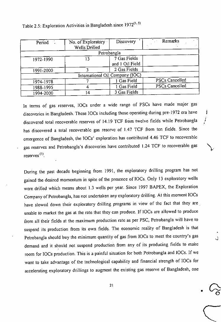
Table 2.5: Exploration Activities in Bangladesh since 1972(1,5)
Period No, of Exploratory . Discovery RemarksWells Drilled
Petrobangla1972-1990 13 7 Gas Fields
and I Oil Field1991-2000 3 2 Gas Fields
International Oil Company (lOC)1974-1978 7 I Gas Field PSCs Cancelled
1988-1995 4 I Gas Field PSCs Cancelled
1994-2000 14 3 Gas Fields
In terms of gas reserves, IOCs under a wide range of PSCs have made major gas
discoveries in Bangladesh, These IOCs including those operating during pre-I 972 era have
discovered total recoverable reserves of 14.19 TCF from twelve fields while Petrobangla
has discovered a total recoverable gas reserve of 1.47 TCF from ten fields. Since the
emergence of Bangladesh, the IOCs' exploration has contributed 4.46 TCF to recoverable
gas reserves and Petrobangla's discoveries have contributed 1.24 TCF to recoverable gas \.
reserves (I)
During the past decade beginning from 1991, the exploratory drilling program has not
gained the desired momentum in spite of the presence of IOCs. Only 13 exploratory wells
were drilled which means about 1.3 wells per year. Since 1997 BAPEX, the Exploration
Company of Petrobangla, has not undertaken any exploratory drilling. At this moment IOCs
have slowed down their exploratory drilling programs in view of the fact that they are.
unable to market the gas at the rate that they can produce. If IOCs are allowed to produce
from all their fields at the maximum production rate as per PSC, Petrobangla will have to
suspend its production from its own fields. The economic reality of Bangladesh is that
Petrobangla should buy the minimum quantity of gas from IOCs to meet the country's gas
demand and it should not suspend production from any of its producing fields to make
room for IOCs production. This is a painful situation for both Petrobangla and IOCs. If we
want to take advantage of the technological capability and financial strength of IOCs for
accelerating exploratory drillings to augment the existing gas reserve of Bangladesh, one
21
• C::o
c

must examine all the options available for the marketing and utilization of thew gas from
the fields discovered and owned by IOCs.
On the other hand GOB has also signed International Power Purchase (IPP) contracts with
international power producing companies for setting up gas based power plants on Build
Owned and Operate (BOO) basis in Haripur, Meghnaghat, Baghabari and Sirajgonj. Some
peaking power plants may also be setup around Dhaka City to meet the peak demand of
Dhaka Metropolis and adjoining areas. The expansion of Gas Transmission Network on the
Western of the Jamuna river using the Multipurpose Bridge has also opened avenues for
setting up gas based industries in the earlier neglected Western region. For ensuring gas
supply in time to all the future power plants and industries, expansion and balancing of the
national grid require to be implemented on priority basis. Otherwise gas transmission
network may have to encounter the same embarrassing situation in the next couple years as
being experienced in the power sector. The constraints of the gas transmission grid require
to be overcome through construction of loop lines and setting up of compressor stations at
strategic locations to expand the capacity of the national gas grid for balancing the system
and ensuring security of supply (2).
2.5.2 Gas Fields of Bangladesh
The first discovery of natural gas was made in 1955 at Haripur (Sylhet Gas Field) and this
was followed by the discovery of the Chhatak Gas Field in 1959. Since then the exploration
of oil and gas resources has led to the discovery of 22 gas fields and one oil field. There are
now 53 producing wells capable of producing about 1300 MMSCFD of gas from 12 gas
fields (I). The locations of gas fields of Bangladesh are shown in Figure2.6.
Cumulative production of gas up to December 2000 was about 4.08 TCF (I). Gas fields of
Bangladesh have Gas initially in Place (GIIP) of about 24.745 TCF. Summaries of gas
initially in place (GIIP) and reserve estimates of different gas fields by Petrobangla are
shown in Table 2.6.
22

GAS TRANSMISSION PIPELINES, GAS FIELDS & OIL FIELD OF BANGLADESH
..<~-Z<.<-••0z
1--
'" -•••~
WEST BENGAL 8akhrabad Franchise AreaTitas franchise AreaJalalabad Franchise Area
Wes Gas Franchise AreaCas Transmission Pipelines
Proposed Transmission Pipelines
Gas FieldOil FiI~ld
AssAM (INDIA)
o•
Figure 2.6: Natural Gas Fields in Bangiadesh (12)
23

Table 2.6: Gas Fields of Bangladesh (I)
Sl. Field ' Year GIIP Recoverable Net Remarks
No. , (proven + Reserve (proven Recoverableprobable) + probable) ReserveTCF TCF TCF
I Bakhrabad 1969 1.432 0.867 0.280 P
2 Habigonj 1963 3.669 1.895 1.077 P
3 Kailashtila 1962 3.657 2.529 2.297 P
4 Rashidour 1960 2.242 1.309 1.114 P
5 Sylhet 1955 0.444 0.266 0.100 P
6 Titas 1962 4.138 2.100 0.317 P
7 Narshingdi 1990 0.194 0.126 0.097 P
8 Meghna 1990 0.159 0.104 0.081 P
9 Sangu 1996 1.031 0.848 0.757 P
10 Saldanadi 1996 0.200 0.140 0.125 P
11 JalaJabad 1989 1.195 0.815 0.763 P
12 Beanibazar 1981 0.243 0.167 0.162 P
13 Begumgoni 1977 0.025 0.015 0.015 NP
14 Fenchugoni 1988 0.350 0.210 0.210 NP
15 Kutubdia 1977 0.780 0.468 0.468 NP
16 Shahbazpur 1995 0.514 0.333 0.333 NP
17 Semutang 1969 0.164 0.098 0.098 NP
18 Bibiyana 1998 3.150 2.401 2.401 NP
19 Moulavibazar 1999 0.500 0.400 0.400 NP
20 Chhatak 1959 0.447 0.268 0.241 PS
21 Kamta 1981 0.033 0.023 0.002 PS
22 Feni 1981 0.178 0.125 0.085 PS
Total 24.745 15.507 11.42
P: Producing, NP: Non-Producing, PS: Production Suspended
Table 2.6 shows that the total GIIP and initial recoverable reserve of Bangladesh are 24.745
TCF and 15.51 TCF, respectively. Out of this reserve, 4.07 TCF has been produced already
(up to February 2001), and the remaining reserve is 11.42 TCF.
These gas fields as shown in Table 2.6 are under the jurisdiction of different gas companies,
both government owned and multinationals. There are today five companies in the country
producing natural gas. These are:
24
i) Bangladesh Gas Fields limited (BGFCL)
ii) Sylhet Gas Fields Limited (SGFL)
iii) Bangladesh Petroleum Exploration and Production Co. Ltd. (BAPEX)
iv) Shell Bangladesh Exploration and Development B.V. (SHELL)
v) UNOCAL Bangladesh Ltd. (UNOCAL)
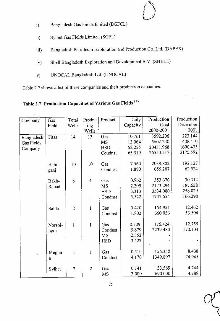
Table 2.7 shows a list of these companies and their production capacities.
Table 2.7: Production Capacities of Various Gas Fields (8)
Company Gas Total Produc Product Daily Production ProductionField Wells mg Capacity Goal December
Wells 2000-2001 2001
Bangladesh Titas 14 13 Gas 10.761 3592.206 223.144Gas Fields MS 13.064 5602.230 408.410Company HSD 52.255 20431.968 1690.435
Condnst 65.319 26553.517 2175.592
Habi- 10 10 Gas 7.560 2039.802 192.127gan] Condnst 1.890 655.207 62.524
Bakh- 8 4 Gas 0.962 353.676 30.312Rabad MS 2.209 2173.294 187.658
HSD 3.313 3534.080 258.029Condnst 5.522 1747.654 166.298
Salda 2 I Gas 0.420 154.951 12.462Condnst 1.802 660.056 53.504
Norshi- 1 1 Gas 0.509 176.424 12.755ngdi Condnst 5.879 2239.480 170.104
MS 2.352 - -HSD 3.527 - -
Meghn 1 1 Gas 0.510 156.350 8.438a Condnst 4.170 1349.897 74.945
Sylhet 7 2 Gas 0.141 53.569 4.744MS 3.000 690.000 4.788
25

Note: Gas: MMSCMD (million standard cubic meter per day), Petroleum Products:
Thousand Liters
Company Gas Total Produc Product Daily Production Production
Field Wells mg Capacity Goal DecemberWells 2000-2001 2001
Sylhet Kerosin 0.178 70.087 5.055
GasFields Kailash 4 4 Gas 2.940 886.121 72.735
Company -tilla MS 19.500 6650.739 611.260
Limited HSD 18.500 _5718.689 525.307Condnst 185.500 76446.347 6556.151
Rashid- 7 6 Gas 4.332 914.444 71.880
pur Condnst 34.534 7687.085 567.879
Biani- 2 I Gas 0.992 35.464 7.156
bazar Condnst 97.388 329.392 679.668
Shell Sangu 6 4 Gas 4.248 1354.933 114.74
B.Y. Condnst 7.155 3337.615 314.680
UNOCAL .Talalaba 4 4 Gas 2.832 854.76 73.465
Bangladesh d Condnst - 59212.240 3731.412
Limited -
Shell and UNOCAL are international oil companies (rOCs) operating under Production
Sharing Contracts (PSC) while BGFCL, SGFL and BAPEX are subsidiary companies of
Petrobangla, the public sector corporation to manage oil and gas resources of the country.
Bangladesh Gas Fields Company Limited (BGFCL) owns eight gas fields, namely, Titas,
Habigonj, Bakhrabad, Narshindi, Meghna, Begumgonj, Feni and Kamta. The productions
from the Kamta and Feni fields are now suspended. The production from the Bakhrabad
field is likely to be suspended in near future. The' Begumgonj field has not yet been
developed (1)
Sylhet Gas Fields Limited (SGFL) owns five gas fields, namely, Haripur (Sylhet),
Kailashtilla, Rashidpur, Beanibazar and Chhatak; and one oil field, namely Haripur. The
production from the Chhatak gas field and the Haripur oil field is now suspended. BAPEX
26
has been given the operatorship of the Saldanadi, Fenchugonj and Shahbazpur gas fields. It
produces gas from Salda Nadi field. Shahbazpur and Fenchugonj fields have not yet been
developed. Shell Exploration and Development B.Y. produces from one field, namely,
Sangu, which is an offshore operation. It also owns two other fields, namely, Semutung and
Kutubdia. Kutubdia is an offshore field (I).
UNOCAL Bangladesh Ltd. owns three gas fields, namely, Jalalabad, Maulavibazar and
Bibiyana. It produces gas from the Jalalabad field (5)
After commencement gas production from Jalalabad and Beanibazar gas field and with the
completion of drilling of additional wells at Rashidpur, Habigonj and Titas Gas Fields, it is
possible to produce 1325 MMCFD of gas from 66 wells of 12 gas fields. Out of the above
amount 630 MMCFD gas can be made available from 6 gas fields of the North- East for
North- South pipe line for onward transmission to national gas grid (2)
2.5.3 Present Demand and Supply Scenario
Natural gas use as a fuel in Chhatak Cement Factory in 1960 with supply from the
Chahatak Gas Field marked its first commercial utilization. It was fed to the first ammonia-
urea grass-roots complex, NGFF at Fenchugonj in 1961 (2). Over the years the consumption
of natural gas has been increasing and its contributed to the national development increased
significantly. Gas production of 24 hours from 12-July-00 to 13-July-OO was 931.262
MMSCF (Daily production report, GTCL, 13-July-OO). In the month on March 2000 the
peak production was lOIS MMSCFD (5). The peak production in 2000 (up to September
2000) was 1089 MMSCFD. On September 18,2001 the production was 1042 MMSCFD and
the two laCs' contribution was "176 MMSCFD (I). The down stream demand and
consumption of natural gas are tabulated in Table 2.8, 2.9, 2.10, 2.11.
27
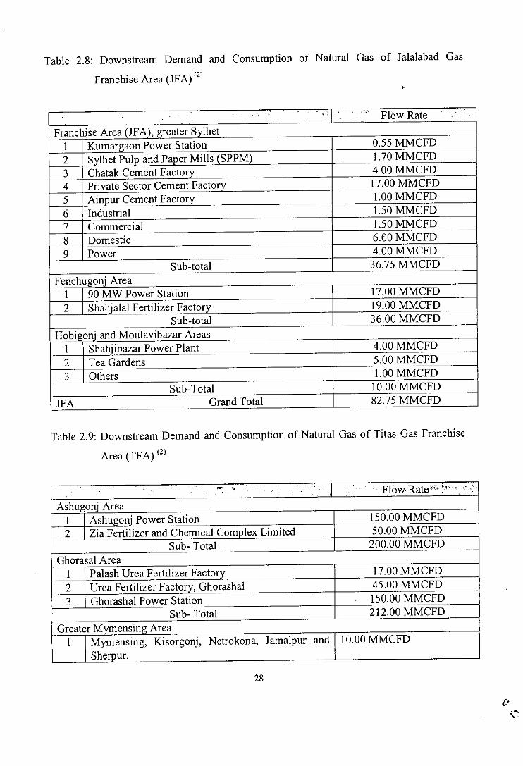
Table 2.8: Downstream Demand and Consumption of Natural Gas of Jalalabad Gas
Franchise Area (JFA) (2)
. , . . , . . ,'. '
c. Flow Rate.
Franchise Area (JFA), greater SvlhetI Kumargaon Power Station 0.55MMCFD
2 Svlhet Pulo and Paper Mills (SPPM) 1.70MMCFD
3 Chatak Cement Factorv 4.00MMCFD4 Private Sector Cement Factory 17.00MMCFD
5 Ainpur Cement Factory 1.00 MMCFD
6 Industrial 1.50MMCFD7 Commercial 1.50MMCFD8 Domestic 6.00MMCFD9 Power 4.00MMCFD
Sub-total 36.75 MMCFDFenchugoni AreaI 90 MW Power Station 17.00MMCFD2 Shahialal Fertilizer Factory I9.00MMCFD
Sub-total 36.00MMCFDHobigoni and Moulavibazar AreasI Shahiibazar Power Plant 4.00MMCFD
2 Tea Gardens 5.00MMCFD
3 Others I.OOMMCFDSub-Total 10.00 MMCFD
JFA Grand Total 82.75 MMCFD
Table 2.9: Downstream Demand and Consumption of Natural Gas of Titas Gas Franchise
Area (TFA) (2)
~ , . ',I FlowRaie'" i", ~':'. . ... , ,
Ashugonj AreaI Ashugonj Power Station 150.00 MMCFD2 Zia Fertilizer and Chemical Comolex Limited 50.00MMCFD
Sub- Total 200.00 MMCFDGhorasal AreaI Palash Urea Fertilizer Factorv 17.00MMCFD
2 Urea Fertilizer Factory, Ghorashal 45.00MMCFD
3 Ghorashal Power Station 150.00 MMCFDSub- Total 212.00 MMCFD
Greater Mvmensing AreaI Mymensing, Kisorgonj, Netrokona, Jamalpur and 10.00 MMCFD
Sherour.
28
,~,.

2 Jamuna Fertilizer Faetorv 43.00MMCFD ,3 RPCL Power Plant 25.00MMCFD
Sub-Total . 78.00 MMCFDGreater Dhaka AreaI Industrial 120.00 MMCFD2 Commercial 20.00MMCFD3 Domestic 80.00MMCFD4 Seasonal 05.00MMCFD
Sub-Total 225.00 MMCFDTFA Grand Total 680.00 MMCFD
Table 2.10: Downstream Demand and Consumption of Natural Gas of Bakhrabad Franchise
Area (BFA) (2)
I . Flow RateBakhrabad Franchise AreaI KAFCO 65.00MMCFD2 CUFL 50.00MMCFD3 2X210 MW Rauian Power Plant 90.00MMCFD4 60 MW and 56 MW Sikalbaha Power Plant 15.00MMCFD5 KPM 8.00MMCFD6 Others 40.00MMCFD
BFA Total 268.00 MMCFD
Table 2.11: Downstream Demand and Consumption of Natural Gas of Western Region
Franchise Area (WFA) (2)
.. I' Flow RateWestern Franchise AreaI 90 MW barge Mounted Power Station 22.00MMCFD2 71 MW PDB Power Plant 21.00MMCFD
WFA Total 43.00MMCFD
Total Gas Demand = 1088.75 MMCFD '" 1089 MMSCFD.
From above tables, it is clear that the present peak demand of the connected down stream
consumer is 1089 MMCFD which can now be met from the current maximum production
capacity of 1300 MMCFD after drawing gas from private producer Shell & UNOCAL. The
situation has improved with the commencement of production from Beanibazar with effect
29
from May 1999. Obviously it is very rare that all the consumers would ever attain peak
concurrently. As such the system peak hovers around 900 to 950 MMCFD which is being
met effectively from national gas grid.
2.5.4 Future Demand and Supply Scenario
International Oil companies which have already commenced production under PSC will
continue their exploration campaign. It is also expected that on achieving significant
discovery followed by appraisal and development additional quantity of gas will be
available for down stream use. UNOCAL in Surma basin (Block 12, 13 & 14) has already
made a significant discovery at Bibyana where two wells have been drilled and a 3-D
seismic survey has been carried out for confirming the ultimate recoverable reserve.
UNOCAL has also discovered a new gas field at Moulvibazar. Shell, UMIC, REXWOOD
are also expected to continue their exploration campaign in their respective blocks. New
discoveries will further enhance our gas reserve.
Sylhet Gas Fields Ltd. (SGFL) under IDA funded Gas Infrastructure Development Project
(GIDP) has completed drilling of 3 wells and installation of required gas treatment plans at
Rashidpur Gas Field. Bangladesh Gas Field Company Ltd. (BGFCL) has also implemented
drilling of 6 additional wells (3 each at Habiganj and Titas Gas Fields) and work over of
some gas wells in these fields. Bangladesh Petroleum Exploration Company (BAPEX) has
also completed drilling second well at Salda. These new wells have provided additional
information about the reservoir of the respective gas fields and have also increased
production by 400-300 MMCFD. On the other hand gas demand is also growing steadily
and is expected to grow significantly over the next couple of years as new power plants will
come into production in Haripur, Meghnaghat and Western side of the Jamuna river.
Government is also planning to set up gas based export oriented fertilizer factories. A
Korean EPZ in Chittagong and industrial parks in Sirajganj, Bogura and Ishwardi also
being set up if supply of gas and stable power can be ensured. For an urea plant having the
production capacity of 5,00,000 tons per year natural gas would require approximately 45
MMCFD. But for adding 100 MW of electricity generation capacity based on natural gas
30

would need about 25 MMCFD additional natural gas. In industrial sector, it will have to
consider the supplemental of existing fuel such as furnace oil and diesel oil in industrial
installation such as boilers and generators plus new industries to be set up. Replacement of
100,000 ton of Furnace oil per year with equivalent quantity of natural gas means an
additional requirement of 12 MMCFD natural gas.
By analyzing the demand and supply situation a projection is made here under the Average
Base Case Supply/Demand which is shown in Table 2.12.
Table 2.12: Average Base Case Supply/Demand (in MMCFD) (2)
.. ' ,' . . ,~
".", ,~{ . Fisca1'Year , .e. c, • ., . ,,~ ,.;:- '~!'.;'", •.', ;, '
"
1998/99 1999/00 2000/01 2001/02 2002/03 2003/04 2004/05
Total Supply 900 1095 1395 1395 1395 1500 1500Total 920 950 1050 1160 1260 1440 1440DemandBalance 20 145 345 235 135 60 60
Table 2.12 indicates that there will be a surplus of 345 MMSCFD in 2000/0 I (2). This is
primarily due to the development of the Rashidpur Gas Field (3 new wells), Habiganj (3
wells) and Titas (3 wells) coming on stream. Utilization of the additional gas will largely
depend on the expansion of the transmission capability of the national gas grid through the
completion of Rashid pur- Ashuganj Gas Transmission Loop line.
It is important to consider that Bangladesh's natural gas resources are concentrated in a few
numbers of big fields (Titas, Habiganj, Rashidpur and Kailashtila) which are at their early
stage of development. Of which there are limited field data are available. It is important to
conducted regular pressure tests in these fields to keep track of their behavior. A prudent
gas supply surplus above average demand should be about 200 MMCFD (2) for the
following reasons:
This will permit temporary shut-in of one or more well of a field at a time in order to
get pressure build up data that are critical for the reservoir management.
31
.P

This amount will allow the temporary loss of production from the equivalent of
nearly a field without causing many difficulties to the consumers.
This amount of surplus should permit taking advantage of the available line pack to
better manage deliveries.
It should be noted that the supply values in the preceding analysis represent short-term
capabilities of the individual fields. These fields are not capable of sustained production for
long at those rates. Several fields have peak supply and average supply at the same level. In
these cases, the fields are not capable of sustained production above average. The Titas
field peak supply and average supply are the same and are at rates lower than current well
capacity. More appraisal drilling is needed, as currently planned, along with systematic
reservior pressure measurements over time wh'ich will allow engineers and geologists to
draw reliable conclusions and to find the strategy to exploited this potential important field.
2.6 Gas Transmission Network
The gas transmission Pipeline in Bangladesh have been planned and constructed targeting a
particular bulk consumer or potential load center. In the early stage of development of gas
sector the grid concept was possibly not visualized. Gas Transmission Company Ltd. And
three transmission and distribution companies are responsible for operation and
maintenance of these transmission pipelines. Over the years, a national gas line grid has
been built and it is connected to lateral and distribution networks. The major gas
transmission lines are described in Table 2.13.
32

Table 2.13: Gas Transmission Network (2)
Gas Transmission Pipelines' Controlling Dianieter (incb) Designed. , .DesignCompany and Length (Km) Operating Capacity
Pressure(MAOP)
Haripur- Fenchugani JGTDCL 8"-25 Km 600 Psi 40MMCFDTangratilla Chhatak JGTDCL 4"-15 Km 750 Psi 30MMCFDShahjibazar - Shamshemagar - Juri JGTDCL 6"-45 Km 600 Psi 40MMCFDValleyTitas - Narshindi - Demra TGTDCL 14"-96 Km 1000 Psi 150MMCFDTitas - Narshindi - Joydevpur TGTDCL 16"/14"-91 Km 1000 Psi 170MMCFDHabigani - Ashugani Trunk Line TGTDCL 12"-38 Km 1000 Psi 88MMCFDBeanibazar - Kailashtilla GTCL 20"-18 Km 1135 Psi IIOMMCFDJalalabad Gas Field- Kailashtilla Unocal 14"-15 Km 1135 Psi 160 MMCFDNorth-South Gas Transmission GTCL 24"-174Km 1135 Psi 330MMCFDPipelineBakhrabad - Demra Pipeline BGSCL 20"-48 Km 1000 Psi 250MMCFDAsguganj - Bakhrabad Gas BGSCL 30"-58 Km 1000 Psi 220MMCFDTransmission PipelineSalda-Bakhrabad Gas Transmission BGSCL 10"-37 Km 1000 Psi 60MMCFDPipelineMeghna-Bakhrabad Gas BGSCL 8"-28 Km 1000 Psi 40MMCFDTransmission PipelineBakhrabad-Chittagonj Gas BGSCL 24"-174Km 960 Psi 350MMCFDTransmission PipelineSangu Gas Transmission Pipeline Shell 20"-45 Km 1135 Psi 240MMCFD
The development of Kailashtilla Gas field in early eighties opened avenues for expansion of
gas transmission network in Sylhet area. A pipeline was built from the Kailashtilla Gas
Field to Chhatak for meeting the demand of that area.
Two more important gas transmission network were developed simultaneously following
the drilling of 11 wells Beanibazar, Kailashtilla, Rashidpur, Habiganj, Titas , Belabo and
Meghna gas fields under second development project.
174 Km. 24" Diameter North-South Pipeline from Kailashtilla- Ashuganj with a
parallel 6" Diameter Condensate/NGL pipeline.
33
v(

117 Km. 24" Diameter Brahmaputra Basin Pipeline from Ashuganj to Elenga for
delivering gas to greater Mymensing areas, Jamuna Fertilizer Factory at Tarakandi
with a future provision for gas supply to the western region of Bangladesh.
The emergence of BGSL created revolutionary changes in the economic development
activities of Southeast. The power plants, fertilizer factories, paper mill, refinery, steel mill
and various other industries of Chittagong region become absolute dependent on gas
available from Bakhrabad as well as Feni gas field. But unfortunately poor production
strategy led to the dramatic decline of gas production from Bakhrabad Gas field and
suspension of gas supply from Feni Gas Field. Under compelling situation due to alarming
sand flow and water production the gas production was drastically reduced causing
suspension of production of Chittagong Urea Fertilizer Factory and some power plants.
This resulted in unbearable load shedding counfrywide. The situation was partially
overcome by expediting construction of 58 Km. 30" Diameter Ashuganj to Bakhrabad Gas
Transmission Pipeline for diverting the surplus gas from the northern Gas Fields to the
Southeast. Subsequently transmission pipelines were also constructed from Meghna Gas
Fields to Bakhrabad and Salda Gas Field to Bakhrabad for augmenting the gas supplies to
the South-East. For flexibility of gas transmission a 20" gas transmission lateral has been
built through Monohordi-Narshigdi-Shiddhirgonj.
18 Km. 20" Beanibazar to Kailashtilla gas transmission pipeline has been constructed and
commissioned in April 1999. 15 Km. 14" gas transmission pipeline from Jalalabad gas
field to Kailashtilla has also been commissioned in February 1999. Transmission pipeline is
also being built along and on either sides of Bangabondhu Jamuna Multipurpose Bridge to
supply gas to the Western Region.
34

Chapter 3
PIPESIM
3.1 Introduction
PIPESIM for Windows is a user-friendly and multiphase software product developed by
Baker Jardine. The PIPES 1M for Windows family of multiphase software consists of:
PIPES 1M for Windows-Single Branch, PIPES 1M-Net, PIPESIM-Goal, HoSIM,
PlPESIM-FPT, WinGLUE (13). In this study PIPES 1M-Net software is used for network
analysis.
3.2 PIPESIM-Net
PIPES 1M-Net is a network analysis model extension to PIPESIM for Windows Single
Branch. Features of the network model include: unique network solution algorithm to
model wells. in large networks, rigorous thermal modeling of all network components,
multiple looped pipeline/flow line capability, well inflow performance modeling
capabilities, rigorous modeling of gas lifted wells in complex networks, comprehensive
pipeline equipment models and gathering and distributing networks.
Baker Jardine's PIPES 1M-Net for Windows is a highly sophisticated but user-friendly
software package for modelling steady state flow in networks. Combining powerful
three phase and thermodynamic analysis methods with rapid convergence algorithms
PIPESIM-Net for Windows will give accurate results in the shortest possible time.
Furthermore, with PIPES 1M-Net for Windows the user can simulate networks having
multiple sources and multiple sinks, flowing compositional mixtures or black oil fluids.
And, since PIPESIM-Net for Windows is truly Microsoft Windows compatible, the user
enjoy multi-tasking, printer sharing, data exchange and all the other benefits of this
operating system.
PIPES 1M-Net allows the users to simulate networks flowing just about any single phase
or two-phase mixture. If the user wish to get up and running quickly then the user can
35("'2->'""-=(

specify different source fluids as a simple black oils. However, the users are also able to
enter full compositional data for each source should the user wish. Furthermore, the
users are free to enter either global fluid properties or completely different fluids at
different sources.
3.3 Black Oil and Compositional Data
The difference between black oils and compositional fluids is that the formers are
approximations to the latter. Black oil fluids are generic fluid models that can be tuned
slightly to match your experimental data, whilst compositional fluids are defined
precisely as consisting of quantities of basic constituents (methane, ethane, glycols,
water etc.). Using a black oil model often requires less computation time than running a
fully compositional model but the user may lose some accuracy. The user may wish,
therefore, to run a black oil simulation first and then complete a compositional
simulation once satisfactory convergence has been attained. PIPESIM-Net for Windows
allows the user to mix black oils or compositional fluids, but the user can not mix black
oil with a compositionally specified fluid.
Before PIPESIM-Net for Windows can be run using rigorous compositional data, a
composition file must be created which contains a component list, quantities and the
equation of state (EOS) to be used. This file contains all input information entered by
the user and so this file can be restored and modified if necessary. Stream components
can be selected fr.om the built-in library, and/or created using the petroleum fraction
prediction utility.
In reality, oil systems contain many thousands of pure components, consisting of a
spectrum of molecules with different carbon numbers and exponentially increasing
numbers of different isomers of each. It would be impossible to model the behavior of
such systems by explicitly defining the amount of each of these molecules, both because
of the excessive computing power needed and the fact that laboratory reports could not
possibly supply all this information. Luckily, since the alkane hydrocarbons are non-
polar and therefore mutually relatively ideal, lumping them together in the form of a .
number of 'pseudo-components' results in fairly accurate phase behavior and physical'
property predictions.
36
" (
3.4 Calibration Data
The PIPESIM-Net for Windows toolbox contains all the components that the user will
need to view and build and edit a network flow sheet, namely; branches, manifolds,
sources and sinks. In PIPESIM-Net the User is able to specify volumetric flow rates at
both sources and sinks. The flow rate specification is made in STOCK TANK or
STANDARD volume units and is applied to the volumetric flow rate of either the gas or
liquid phase depending on whether the User chooses a GAS RATE or a LIQUID RATE.
The ability in PIPES 1M-Net to specify Stock Tank flow rates is exceedingly convenient
for most Petroleum Industry applications since flow rates of hydrocarbons are normally
reported at Stock Tank conditions. However, it is important to remember that
specifying flow rate in this way increases the chance of the user providing PIPESIM-Net
with a set of unphysical specifications.
It is possible for users to specify PIPESIM-Net problems that have no physically
reasonable solution. Such a set of specifications is termed a set. of unphysical
specifications. If the user supplies such a set then PIPESIM-Net will attempt to find the
solution. It will usually fail, however, because its algorithms are designed to look only
for physically reasonable solutions. An example of unphysical specifications would be
a pressure and flow rate specified at the entrance to a pipeline that causes the fluid to
"run-out" of pressure before the outlet of the pipeline.
37

3.5 Model Overview
PIPESIM-Net for Windows follows Baker Jardine's PIPES 1M-Net 2.01, which itself
was designed as a logical extension to PIPES 1M, a successful point-to-point pipeline
simulator. It is a powerful commercial software to solve just about any possible
multiphase network, and also retains most of the functionality. of both DOS PIPES 1M
and PIPES 1M for Windows. PIPES 1M-Net for Windows allows the user unlimited
flexibility with regard to type of problem (13):
• unlimited number of source and sink nodes (max. 256 branches)
• reverse flow if boundary conditions so dictate
• any number of branches connected to a particular node
• loop, crossover and recycle specifications
• in-line flashing of black oil and compositional streams
Hence, it is possible to solve any of the three generic network types, which is shown in
Figure 3.1.
I) Gathering 2) Distribution 3) Looped
Figure 3.1: Types of Network used in PIPESIM-Net
38

3.6 Network Validation
All computers modelling software requires a certain amount of physical data before
simulation can proceed. PIPES1M-Net for Windows is no different in this respect since
the solving of a network requires that values specified for pressure, flow rate and
temperature around the system will allow a solution. The criteria that must be satisfied
when seeking to model any network with PIPES 1M-Net for Windows can be
summarized as follows:
The connectivity of the network must be defined
The fluid composition at all sources must be defined
At least one pressure must be specified somewhere in the system.
The total number of boundary conditions must equal the total number of lone
nodes. This means that the number of flow, pressure and flow versus pressure
curves (inflow performance relationships) that the users specify must equal the
number of sources and sinks in the network.
3.7 Flow Correlations
Single-phase correlations are, as the name, implies, used by PIPES 1M-Net for Windows
for the simulation of pure gas or pure liquid i.e. not multiphase conditions. A number of
correlations are available including Moody and AGA (for dry gas). P1PES1M-Net for
Windows provides the user with a multitude of multiphase pressure drop and holdup
correlations for Horizontal and Vertical Flow Correlations.
3.7.1 Horizontal Flow
The following horizontal flow correlations are currently available in P1PES1M-Net for
Windows
Duns & Ros
Beggs and Brill (Original)
Beggs and Brill (Revised)
Oliemans
No Slip
Mukherjee and Brill
Dukler (AGA and Flanagan)
Mukherjee and Brill
39
Swap Angle is an angle (default 45 degrees) above which horizontal flow correlations
are used.
3.7.2 Vertical Flow
The following vertical flow correlations are currently available 111 P1PES1M-Net for
Windows
Duns and Ros
Beggs and Brill (Original)
Baker Jardine (Revised)
Orkiszewski
Hagedorn and Brown
No Slip
Govier, Aziz and Fogarasi
Mukherjee and Brill
Gray
3.7.3 Single Phase Correlations
Several single-phase pressure drop correlations are available for both liquid and gas
based systems. PIPES 1M will automatically select either the specified two-phase or
single-phase correlation depending on the phase behaviour at the particular section in
the pipeline. The single-phase correlation is set by default to the MOODY correlation.
So, by default if single-phase flow is encountered in the system, the program will
automatically switch to the MOODY correlation. The available single-phase
correlations are briefly described below:
Moody: At Reynolds numbers greater than 2000, the Moody correlation uses the
Colebrook-White equation (Moody chart) and at Reynolds numbers less than
2000, assume laminar flow (f=64/Re). (Default).
AGA: Known more fully as the AGA Gas correlation. This is the recommended
correlation for single-phase gas based systems.
Panhandle 'A': Empirical gas based correlation. Limited range of applicability. AGA
or Moody correlation recommended.
40

Panhandle 'B': Empirical gas based correlation. Limited range of applicability. AGA
or Moody correlation recommended.
Weymouth: Empirical gas based correlation. Limited range of applicability. AGA or
Moody correlation recommended.
In addition to the above, a number of sophisticated new correlations (e.g. mechanistic
models) are available as optional extras to PIPES 1M for Windows. These correlations
are the result of extensive research and development in multiphase flow laboratories
worldwide.
3.8 Convergence
PIPES 1M-Net for Windows uses a GNET algorithm to solve all networks. Reaching a
solution involves continually estimating and refining a matrix of results for each branch
while simultaneously taking into consideration the many sources of discontinuity within
the network. These sources of discontinuity' include, dead wells, two phase vertical
flow, critical flow, phase changes and flow regime boundaries.
By default the tolerance for PIPESIM-Net for Windows simulations is set to 0.01.
Mathematically this means that the .simulation will terminate when the root mean square
error for pressure at the junction node having the greatest root mean square pressures
error is less than 0.01. If the user decrease this value then the user are forcing
PIPESIM-Net for Windows to do more calculating and produce more accurate results.
PIPESIM-Net for Windows will by default complete a maximum of 100 iterations per
simulation. If after 100 iterations no solution meeting the required tolerance has been
found then PIPESIM-Net for Windows will stop and display existing results. If the user
find that a particular system is not converging then, generally, it is best to relax the
tolerance rather than increase the maximum number of iterations.
PIPESIM-Net for Windows makes use of convergence techniques that are tuned to suit
each individual problem. These routines are based on well-accepted mathematical
theorems but modified to allow for the discontinuities that might be generated by
different flow correlations, as well as those originating from the problem specification.
41

Chapter 4
GAS TRANSMISSION SYSTEM AND RELATED DATA
4.1 Introduction
The gas transmission pipelines in Bangladesh were initially planned and constructed
targeting particular bulk consumers or potential load centers. In the early stage of the
development of the gas sector, the grid system was possibly not visualized.'But over the
years the gas transmission system has expanded considerably and has become
complicated. Four Companies of Petrobangla such as Gas Transmission Company Ltd.
(GTCL). Titas Gas Transmission and Distribution Company Ltd. (TGTDCL),
Bakhrabad Gas System Ltd. (BGSL). Jalalabad Gas Transmission and Distribution
System Ltd. (JGTDSL) and two international coinpanies (Unocal Bangladesh Ltd .. Shell
Bangladesh Exploration and Development B.V.) are responsible for operation and
maintenance of their respective transmission pipelines (Chapter 2). The locations of
existing transmission lines (with future extension) were shown in Figure 2.6.
4.2 Network Analysis
A geographical breakdown of the demand is a prerequisite to any analysis of a
transmission network. In order to reliably cope with the gas transmission constraints and
more specifically with the maximum flow rates to transfer through the pipelines, the
geographical breakdown must go beyond the traditional split in four areas Ti las
Franchise Area (TFA). Bakhrabad Franchise Area (BFA), Jalalabad Franchise Area
(JFA). and Western Franchise Area (WFA) which are respectively under the
responsibility of TGTDCL, BGSL, JGTDSL, GTCL. The eight areas (Figure 4.1)
correspond to a compromise between a significant level of actual demand with a
dominant focal point for the demand, meaning that the necessary links (gas pipelines)
between areas are reasonably identified (9L
Area I: Western zone
42
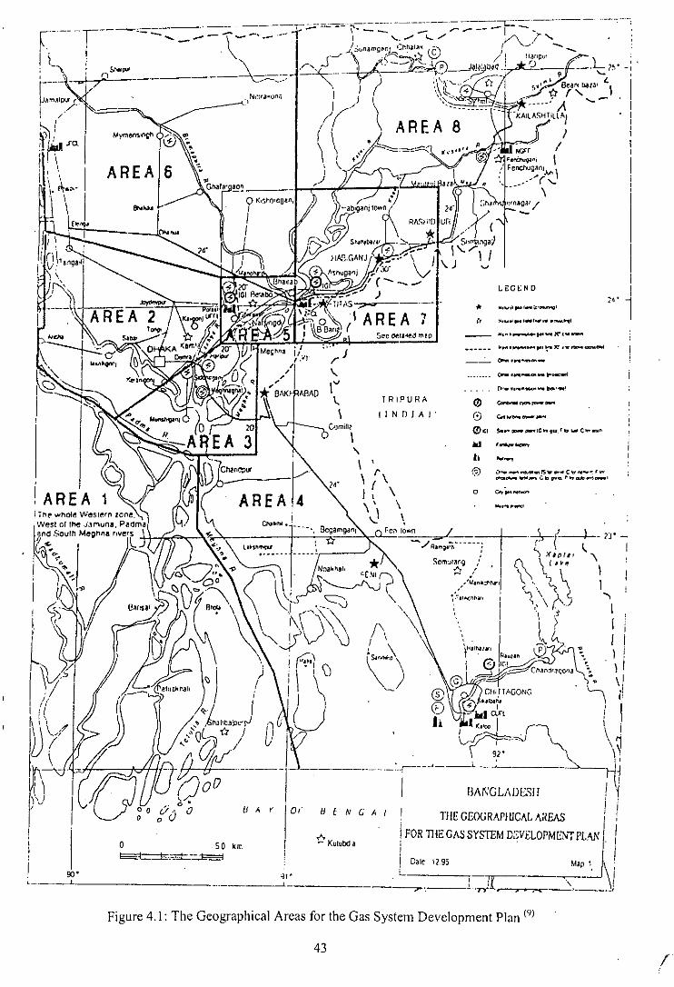
LEa~ND
eor- ••.• _ •••••.• IP_I
S.",_",lC'"fU.rv ••••C"'_"
.,. •• __ ••••• rs"' ••.•• C •••.•• _"' ••..•.1I'a__ ••.• C,,"II"" .b •••••••••.'_'
....... ~.
,--
•. ••••..i'''. '•.•""""""'V'
o
G c... ••.__ •..
__ ~••••_ •.••••••1I!1"_
TR1PUAA
I I N D I A I'
BENGAl
-C:r Kulubd a
U A Y
"'': I t \,/"'"."~.'I <,; " I
~."""'-;~~oII' I '1.. \ At."'"1 "\'j') II 'I > ( i, I ' I" I .!.' to. I 1
'\1-<'11'11/'" I pj 1 i"'ulin Y ,
I .21~"o,,,,o,,, 0 '\ 1
@ ~~. '),,' \1,,1,@ CHI.' TAGONG\~ \ ~ •.,fbi'" '
CD V - ••• e&l ! !It I I",;" I, I-",-,~I" \~
\ 91' \ \,'----~-~iIlA1':GL,\DESI! I I
I TilE GE()(;RAPIUCAL A;lEAS ; :! FOR TIlE GAS SYSTEM D:,Vt:LOPMENT PIAN I Ii jl~ Calc \295 Map~, \,
"l~ --- I______ .-l_. ~-,---: ..Jr. >; ."'C '.'_-=-_ . .:i
o SO kIT'.
Ei£L:::b:~=-
00'I
Figure 4.1: The Geographical Areas for the Gas System Development Plan (9)
43/
Area 2: Dhaka (the greater Dhaka non-bulk market)
Area 3: Meghna (mainly three power stations)
Area 4: Bakhrabad-Chittagong (the BFA gas market)
Area 5: Ghorasal (mainly the power station and two fertilizer plants)
Area 6: Brahmaputra (mainly a fertilizer factory)
Area 7: Titas-Ashugonj (mainly the power plant and fertilizer plant)
Area 8: Sylhet (the .lFA gas market and the ultimate excess gas resources)
The main high-pressure lines of Bangladesh are shown in Figure' 4.2. Possible
extensions in Western zone are also shown in Figure 4.3.
Network analysis is a complex process. In this study, the gas transmission network is
analyzed with the help of PIPES 1M-Net. To simulate the network the following
information was required:
i) Source temperature, pressure/ flow rate
ii) Composition of natural gas of sources
iii) Pipe diameter, length, thickness, roughness, ambient temperature
iv) Minimum one source/ load pressure
The required data is collected from GTCL, .lGTDSL, TGTDCL, and UNOCAL
Bangladesh Ltd. All required data are available except pipe thickness and roughness.
Therefore, it is assumed that pipe thickness and roughness of pipe are 0.5 inch and
0.0006 respectively. The ambient temperature is changed with the season and place. The
. assumed ambient temperature is 25°C because of unavailability of data. The source
temperature of Kailashtilla gas field is 110°F and .lalalabad gas field is 83°F. The
temperature of other fields varies from 95°F to 110°F. In this simulation, the source
temperature of other fields is considered to be 100°F. The Weymouth equation, AGA
equation and Moody equation are used to simulate the network. To convergence the
simulation, maximum 11 % tolerance is used. But most of the cases the tolerance is
below 10 % only.
44

(INDIA)
BANGLADESH
GAS TRANSMISSION NETWORK
,..
\,'"\I'"\
I\I1I\I
23"
-
Map B
I\\
TRIPURA
r,- r,oJ " I,
\\\II
v
rII\
J",/
I(\\,"
Dale 12.95
See delalled map 9
ComJlIa ,"24", 115km
\ '\1(\\ \ \
",' \Feni lown
-./ R'l\'Ig~------l
SemUlarlg ,/
*/~/M.n~n
-'\ F.:JIl::M ••.,
\,\\ H.'hUItI
I T'
'IT,59kn,J\,\"l-I
-- ..•......_-------
'8 A Y OF 8 E N G A L
0 SO ,•. f:r Kutubdia'-
",. g, •,
Figure 4.2: Gas Transmission Network Main High Pressure Lines in Bangladesh (9)
45
,•

,r'")(
l h •••.w.
l,Jessore
~"\I...•,,I\
\.
\\\
-
TRIPURA
~.••r\J " I,,
\\\\
( I N D I A I
v
rI\\I
.//
I(,,,/
-/;''''{lI~-----7Semutang .'
tr /,,/1c.nIo;::l'Ilwll
~F.~,\,
"\
See delailed map
Camilla
\"-\, ",I ( ," ,\,., \
Feni Iown
~
J~f.,
161020"" \::a
62km
• 2.',165km, IBh,!IIam8f8 to Khulna I
""
Possible ~o,ec1in 2010
,."(
r.//
",.•.•..r-1I/
r',,r_,I
5' d' ~,.N !il, 0il: ~ &;I, ~ ~= 15 r-s' >er !l5 tl~ 0 f:l:E z ;c~~3
•...~ 0 0= ~~"
"
]
"."<"'""3;>:l"er3.o"
z"~o~"'"0o'"'"cr:"rnx""'"0'"
oI;:-1i3"'"3'"'"o"
>-c1~.(l..,.w
..,.e;,

Table 4.1: Chemical Composition of Natural Gas in Different Gas Fields (151
NP = Non-producing A = AbandonedN.B. P = Producing
SL Name of Chemical Composition of Gas (Volume Percent) Caloric Specific Remarks
No Gas Fields Value GravityMethane Ethane Propane i-Butane n-Butane High Nitrogen Carbon Gross
Composition Dioxide BTU/CFT
A UnderBGFCL1. Bakhrabad 94.20 3.65 0.72 0.20 0.10 0.24 0.42 0.47 1057.73 0.5970 P
2. Begumganj 95.46 3.19 0.64 0.17 0.04 0 0 0.30 1045.61 0.5833 NP
3. Belabo 94.79 2.49 0.60 0.20 0.15 0.13 0.34 0.60 - 0.6070 P
4. Feni 95.71 3.29 0.65 0.15 0.05 0 0 0.15 1049.84 0.5782 A
5. Habigoni 97.60 1.31 0.27 0.08 0.04 0.06 0.38 0.07 1023.91 0.5700 P
6. Kamta 95.36 3.57 0.47 0.09 0 0 0 0.51 1043.13 0.5743 A
7. Me£hna 95.15 2.83 0.60 0.16 0.09 0.07 0.37 0.53 - 0.5910 P
8. Titas 97.33 1.72 0.35 0.08 0.05 0.06 0.30 0.11 1031.55 0.5720 P
9. Shabbazpur 93.68 3.94 0.71 0.20 0.07 0.04 0.46 0.90 1046.21 0.5800 NP
10. Saldanadi 96.32 2.16 0.45 0.12 0.07 0.05 0.27 0.56 1032.60 0.5700 P
B UnderSGFL1. Beanibazar 93.68 3.43 1.10 0.29 1.23 0.17 0.99 0.12 1061.95 1.600 P
2. Chattak 97.90 1.80 0.20 0 0 0 0 0 1005.71 0.548 A
3. Fenchu£anj 95.66 2.50 0.63 0.11 0.04 0 0 0.06 1043.33 0.5740 NP
4. Haripur 96.63 2.00 0.05 0.14 0.01 0.17 0.66 0.34 1050.68 0.546 P
5. Kailashtilla 95.57 2.70 0.94 0.21 0.20 0.14 0.24 0 1056.00 0.5860 P
6. Rashidour 98.00 1.21 0.24 0 0 0.17 0.02 0.05 1012.00 0.5690 P
C Under International Oil Companies1. Jalalabad 93.50 3.50 1.30 0.20 .80 0.20 0.30 0.50 - - P
2. Kutubdia 95.72 2.87 0.57 0 0.31 0 2.36 1041.66 0.5860 NP
3. Sangu 94.51 3.17 0.61 0.19 0.07 0.41 2.44 1061.00 0.5900 P
4. Semutan£ 96.34 1-....-1.70 0.14 0 0.01 0 0.86 - - NP
N.B. BAPEX has been given the operator-ship of the Shahbazpur and Salda Nadi fields.
'\(
47
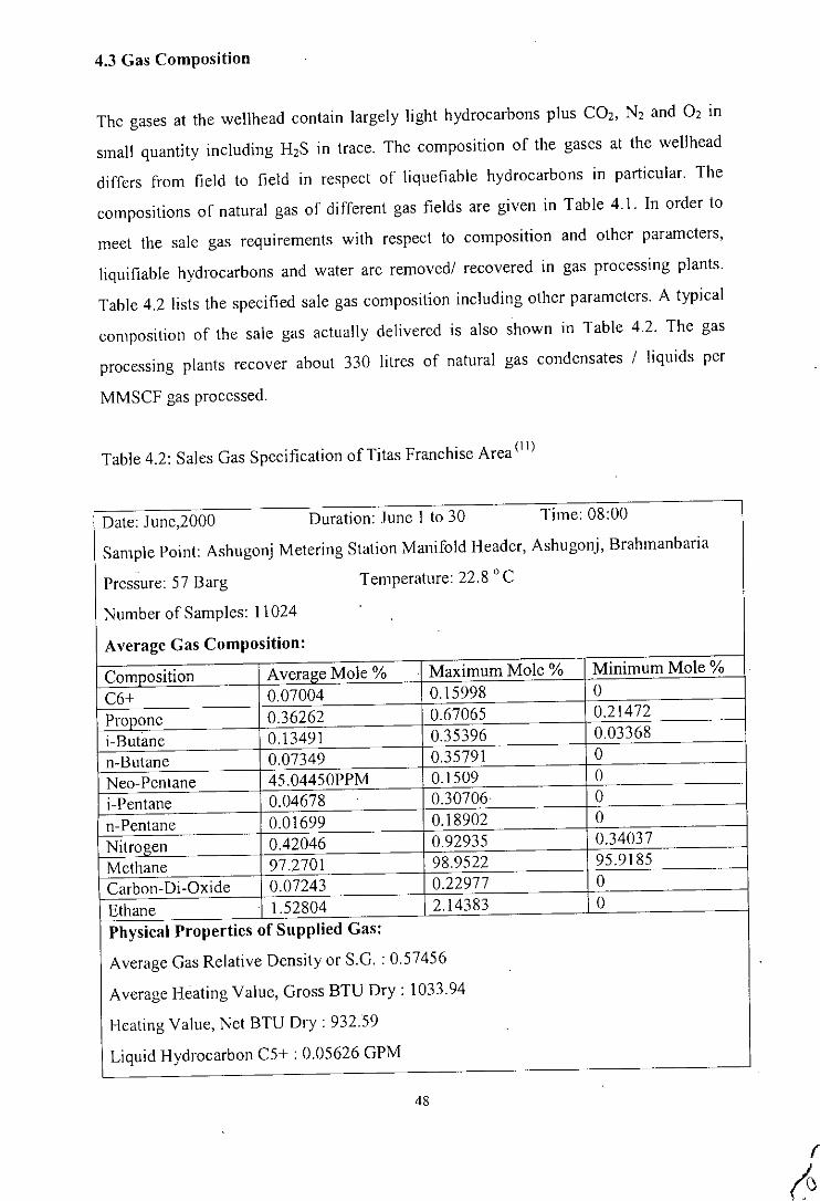
4.3 Gas Composition
The gases at the wellhead contain largely light hydrocarbons plus CO2, Nz and O2 in
small quantity including HzS in trace. The composition of the gases at the wellhead
differs from field to field in respect of liquefiable hydrocarbons in particular. The
compositions of natural gas of different gas fields are given in Table 4.1. In order to
meet the sale gas requirements with respect to composition and other parameters,
liquifiable hydrocarbons and water are removed/ recovered in gas processing plants.
Table 4.2 lists the specified sale gas composition including other parameters. A typical
composition of the sale gas actually delivered is also shown in Table 4.2. The gas
processing plants recover about 330 litres of natural gas condensates / liquids per
MMSCF gas processed.
Table 4.2: Sales Gas Specification ofTitas Franchise Area (II)
Date: June,2000 Duration: June 1 to 30 Time: 08:00
Sample Point: Ashugonj Metering Station Manifold Header, Ashugonj, Brahmanbaria
Pressure: 57 Barg Temperature: 22.8 0 C
Number of Samples: 11024
Average Gas Composition:
Composition Average Mole % Maximum Mole % Minimum Mole %
C6+ 0.07004 0.15998 0
Propone 0.36262 0.67065 0.21472
i-Butane 0.13491 0.35396 0.03368
n-Butane 0.07349 0.35791 0
Neo-Pentane 45.04450PPM 0.1509 0
i-Pentane 0.04678 0.30706 0
n-Pentane 0.01699 0.18902 0
Nitrogen 0.42046 0.92935 0.34037
Methane 97.2701 98.9522 95.9185
Carbon-Di-Oxide 0.07243 0.22977 0
Ethane 1.52804 2.14383 0
Physical Properties of Supplied Gas:
Average Gas Relative Density or S.G. : 0.57456
Average Heating Value, Gross BTU Dry: 1033.94
Heating Value, Net BTU Dry: 932.59
Liquid Hydrocarbon C5+ : 0.05626 GPM
48
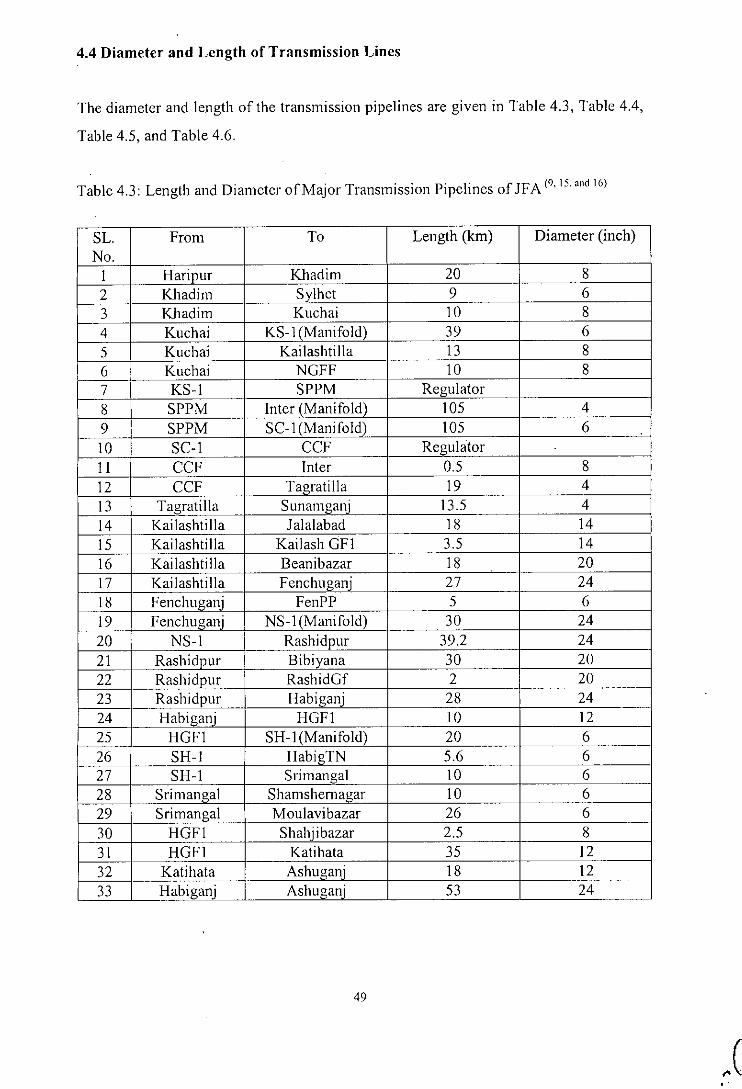
4.4 Diameter and Length of Transmission Lines
The diameter and length of the transmission pipelines are given in Table 4.3, Table 4.4,
Table 4.5, and Table 4.6.
Table 4.3: Length and Diameter of Major Transmission Pipelines of JFA (9.15. and 16)
SL. From To Length (kIn) Diameter (inch)No.
1 Haripur Khadim 20 82 Khadim Sylhet 9 63 Khadim Kuchai 10 84 Kuchai KS-1 (Manifold) 39 65 Kuchai Kailashtilla 13 86 Kuchai NGFF 10 87 KS-l SPPM Regulator8 SPPM Inter (Manifold) 105 49 SPPM SC-1 (Manifold) 105 610 SC-1 CCF RegulatorI 1 CCF Inter 0.5 812 CCF Tagratilla 19 413 Tagratilla Sunamganj 13.5 414 Kailashtilla Jalalabad 18 1415 Kailashtilla Kailash GFI 3.5 1416 Kailashtilla Beanibazar 18 2017 Kailashtilla Fenchuganj 27 2418 Fenchllganj FenPP 5 619 Fenchllganj NS-1 (Manifold) 30 2420 NS-l Rashidpur 39.2 2421 Rashidpur Bibivana 30 2022 Rashidpur RashidGf 2 2023 Rashidpur Habiganj 28 2424 Habigani HGFI 10 1225 HGFI SH-I (Manifold) 20 626 SH-J HabigTN 5.6 627 SH-I Srimangal 10 628 Srimangal Shamshemagar 10 629 Srimangal Moulavibazar 26 630 HGFI Shahjibazar 2.5 831 HGFJ Katihata 35 1232 Katihata Ashllgani 18 1233 Habigani Ashugani 53 24
49
..

Table 4.4: Length and Diameter of Major Transmission Pipelines ofTFA (9. 16)
, SL. From To Length (km) Diameter (inch)No.34 TitasGF Bbaria I 1235 BBaria TN-I (Manifold) I 1436 BBaria TN-2(Manifold) I 1637 TN-I TN-3(Manifold) 21.1 1438 TN-2 TN-4(Manifold) 45 1639 TN-3 Narshindi 30 1440 TN-4 Narshindi I 1641 Narshindi Ghorasal 8.4 1442 Narshindi Demra 32 1443 Narshindi Shidd 45 2044 Narshindi BelaboGF 13 845 Shidd .T27(Manifold) 10 1046 J27(Manifold) Demra 10 1447 Demra Gulshan 32 1448 Gulshan Joydevour 25 1249 Joydevpur Elenga 56 1050 Ashllganj Daulatkandi 9 2451 Daulatkandi Daulot#(Manifold) 0.1 1252 Daulatkandi Monohordi 25 2453 Monohordi Elenga 89 2454 Monohordi Kishorganj 36 455 Monohordi Narshindi 32 2056 Dhanua Mymen 63.004 1257 Mymen Netrokona 32.5 6
Table 4.5: Length and Diameter of Major Transmission Pipelines of BFA (9. 16)
SL. Length (km) Diameter (inch)No.
58 Ashllganj Bakharabad 57.1 3059 Bakharabad Falljdar 171.5 2460 Bakharabad Dewanbag 60 2061 Sangu Falljdar 49 2062 Falljdar Chittagoni city 2.5 2463 Dewanbag Demra 8 2064 Dewanbag HariPP 1.58 1465 Bakharabad Salda 35 1066 Bakharabad Meghna. 28 867 Bakharabad BakharabadGF I 20
50
I\.

Table 4.6: Length and Diameter of Major Transmission Pipelines of WFA (9. 16)•
SL. Length (km) Diameter (inch)No.68 Elenga .fB1(Manifold) 15 2469 .fBI .fB2(Manifold) 9 30
70 .fB2 Nolka 15 24
71 Nolka . Sira;gonj 5 2072 Nolka Bbari 43 20
73 Nolka Ishurdi 65 24
74 Ishurdi Bheramara 25 2475 Bheramara Kuatia 15 2476 Kustia Jhenaidha 20 2477 Jhenaidha Jessore 50 2478 Jessore Khulna 64 24
51
Chapter 5
STEADY- STATE FLOW OF GAS THROUGH PIPES
5.1 Introduction
Pipes provide an economIc means of producing (through tubing or casing) and
transporting (via flow lines or pipelines) fluids in large volumes over great distances.
They are convenient to fabricate and install, and provide an almost indefinite life span.
Because flow is continuous, minimal storage facilities are required at either end (field
supply end, and the consumer end). Operating costs are very low, and flow is guaranteed
under all conditions of weather, with good control (an installed pipeline can usually
handle a wide range of flow rates). There are no spillage or other handling losses. unless
the line develops a leak, which can be easily located and fixed for surface lines. The
flow of gases through piping systems involves flow in horizontal, inclined, and vertical
orientations, and through constrictions such as chokes for flow control. This chapter
introduces some basic concepts of horizontal flow types.
5.2 Gas Flow Fundamentals
All fluid flow equations are derived tl'om a basic energy balance which, for a stcady
state system (no time dependence offlow parameters), can be expressed as:
Change in internal energy + Change in kinetic energy + Change in Potential energy +
Work done on the fluid + Heat energy added to the fluid - Shaft work done by fluid on
the surroundings = 0
Thus, on a unit mass basis, the energy balance for a fluid under steady - state flow.
conditions can be written as:
dv' g .dU+-+-dz+d(pV)+dQ-dw, = 0
. 2g, g, ................... (5.1)
It is converted into a mechanical energy balance using the well-known thermodynamic
relations. For an ideal process. Equation 5.1 becomes:
52

d 2
Vdp+ _V_ + JLdz + df" - dw, = 02g, g,
. .... . . .. . ; .. .. .. . (5.2)
........................... (5.3)
Neglecting the shaft work ws, and multiplying throughout by the fluid density, p:
dp + pdv' +JL pdz + pdf" = 02g, g,
All the terms in Equation 4.4 have units of pressure. Equation 4.4 can also be written as:
.............. (5.4)
where 6pl' represents the pressure drop due to friction, and is independent upon the
prevailing flow conditions.
5.3 Types of Single-Phase Flow Regimes and Reynolds Number
Four types of single-phase flow regimes are possible: laminar, critical, transition and
turbulent. Reynolds applied dimensional analysis to flow phenomena, and concluded
that the flow regime that will prevail is a function of the following dimensionless group
known as the Reynolds number, NR,:
N' = inertia - forcesR, V' fiISCOUS - orces
upd 4qp--=--
..................................................... (5.5)
For most practical applications, the Reynolds number for a gas is given by:
20q"Yg
N R, '" -f.l-d-
Where, q" is in mscfd, f.l is in cp and d is in inches.
As shown in the Moody fi'iction factor chart, flow regime is related to Reynolds number
as follows (171;
Flow type N Re, smooth pipes
------------ ----------------------Laminar <2000
Critical 2000-3000
Transition 3000-4000
Turbulent >4000
53

5.4 Pipe Roughness
Friction to flow through a pipe is affected by pipe-wall roughness. However, pipe
roughness is not easily or directly measurable, and absolute pipe roughness E is,
therefore, defined as the mean height of protrusions in uniformly sized, tightly packed
sand grains that give the same pressure gradient as the given pipe. This roughness may
change with pipe use and exposure to fluids. Some typical values for roughness are
shown below (IS!:
Types of pipe
Drawn tubing (brass, lead, glass)
Aluminum pipe
Plastic-lined or sand blasted
Commercial steel or wrought iron
Asphalted cast iron
Galvanized iron
Cast iron
Cement-lined
Riveted steel
E
0.00006
0.0002
0.0002-0.0003
0.0018
0.0048
0.006
0.0102
0.012-0.12
0.036-0.36
Commonly used well tubing and line pipe:
New pipe 0.0005-0.0007
12-months old 0.00150
24-months old 0.00175
From dimensional analysis, it has been deduced that relative roughness, the ratio of the
absolute roughness and inside pipe diameter, E/d, rather than absolute roughness, affects
flow through pipes.
54

5.5 Pressure Drop Calculations
pipeline (a pump, compressor, turbine etc.), this equation is readily integrated to yield
g pAu' 2!fpu'dlp,_p, =_ p6.z+--+--- (5.7)g, 2e, g,d
The pressure drop over a distance, L, of single-phase flow in a pipe can be obtained by
solving the mechanical energy balance equation, which in differential form is (\7)
dp udu g 2!fu'dl_ +_ +-dz +_'---.+ dW, =0 (5.6)P g, g, g,d
If the fluid is incompressible (p= constant), and there is no shaft work device in the
~=~~+~u+~ •...: (5.~
for fluid moving from position I to position 2. The three ten11Son the right-hand side
are the potential energy (PE), kinetic energy (KE) and frictional contributions to the
overall pressure drop, or
5.5.l The Pressure Drop due to Potential Energy Change (ApPE)
API'Eaccounts for the pressure change due to the weight of the column and fluid (the
hydrostatic head); it will be zero for flow in a horizontal pipe. From Equation (5.7), the
potential energy pressure drop is given by:
gApl'!' = -p6.z ., (5.9)g,
5.5.2 The Pressure Drop due to Kinetic Energy Change (ApKE)
ApKEis the pressure drop resulting from a change in the velocity of the fluid between
positions I and 2. It will be zero for an incompressible fluid unless the cross-sectional
area of the pipe is different at the two positions of interest. From Equation (5.7),
API'E=L(Au,)=L(u: -u~)= 8~g2 (~-~J (510)2g, 2g, J[ g, ld, d,
55

5.5.3 The Frictional Pressure Drop ("'PF)
The frictional pressure drop is obtained from the Fanning equation,
21fpu21"'PF =-~- (5.11)
g,d
where, fr is the Fanning friction factor. Usually, the Moody friction factor is used. The
friction factor includes, besides roughness, the flow characteristics of the flow regime. It
is therefore a function of Reynolds number and relative roughness:
where, k is the length of the protrusions on the pipe wall.
In laminar flow, the friction factor is a simple function the Reynolds number,
16If =- (5.12)NRC
In turbulent flow, the friction factor depends on both the Reynolds number and the
relative pipe roughness.
The Fanning friction factor is most commonly obtained from Moody friction factor
chart. This chart was generated from the Colebrook-White equation (191,
k = -410g( 3.7~65 +~r~P;J (5.13)
The Colebrook-White equation is implicit in fr, requiring an iterative procedure, such as
the Newton-Raphson method, for the solution. An explicit equation for the friction
factor with similar accuracy to the Colebrook-White equation is the Chen equation (I"!:
S6
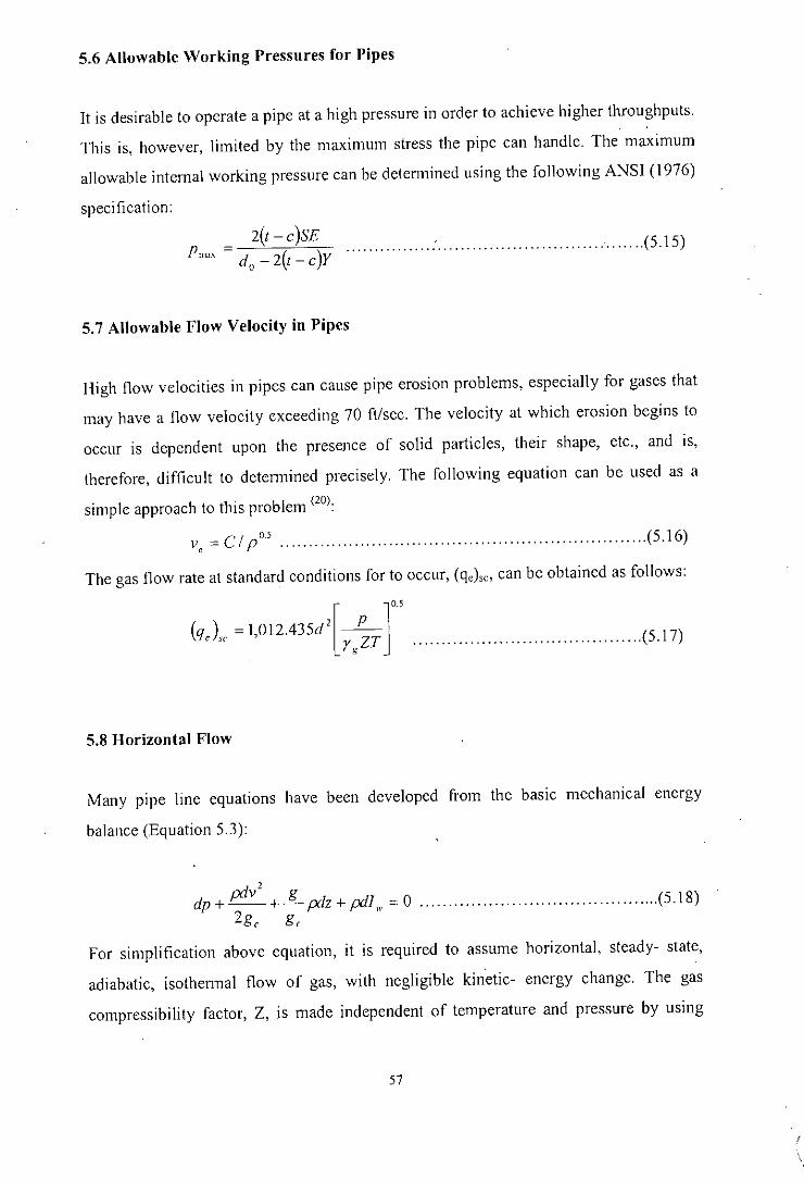
5.6 Allowable Working Pressures for Pipes
It is desirable to operate a pipe at a high pressure in order to achieve higher throughputs.
This is, however, limited by the maximum stress the pipe can handle. The maximum
allowable internal working pressure can be detennined using the following ANSI (1976)
specification:
2(1-e)SEPmax = do - 2(t - c)Y
............... : (515)
5.7 Allowable Flow Velocity in Pipes
High flow velocities in pipes can cause pipe erosion problems, especially for gases that
may have a flow velocity exceeding 70 ft/sec. The velocity at which erosion begins to
occur is dependent upon the presence of solid particles, their shape, etc., and is,
therefore, difficult to determined precisely. The following equation can be used as a
simple approach to this problem (20!;
v, =C/ p05 ....•........................................................... (5.16)
The gas flow rate at standard conditions for to occur, (qe)", can be obtained as follows:
I ]0.5(q,t = 1,012.435d'lr g~T (5.17)
5.8 Horizontal Flow
Many pIpe line equations have been developed from the basic mechanical energy
balance (Equation 5.3):
pdv' gdp + -- + - pdz + pdf" = 0 (5.18)2g, g,
For simplification above equation, it is required to assume horizontal, steady- state,
adiabatic, isothennal flow of gas, with negligible kinetic- energy change. The gas
compressibility factor, Z, is made independent of temperature and pressure by using
57
,,

average compressibility factor, Zav, for simplicity. Integrating Equation 5.18 over the
pipe length from 0 to L and pressure PI to Pz, we have:
(
2 )(( 2 2 ~5 J2 _ Rg,T"PI - P2q" - 49.9644 P~, rgZ"TfL
ln common units, Equation 4.19 becomes:
5.8.1 Non-Iteration Equations for Horizontal Gas Flow
i) Weymouth Equation (17)
........................... (5.19)
.............. " (5.20)
Weymouth proposed the following relationship for friction factor as a function of pipe
diameter d in inches:
f = 0.0032/ dl"
......................... : (5.21)
Substituting for f from Equation 5.21 in Equation 5.20:
.......................... (5.22)
This is known as Weymouth for horizontal flow. It is used most often for designing gas
transmission systems because it generally maximizes pipe diameter requirements for a
given flow rate and pressure.
ii) Panhandle (Panhandle A) Equation (17)
This equation assumes that fis a function of Reynolds number as follows:
f = 0.0768/ N~~14(" ...... :. (5.23)
Substituting for f from Equation 4.23 in Equation 5.20:
......................... (5.24)
The Panhandle A equation is most applicable to large diameter pipelines, at high flow
rates.
58

iii) Modified Panhandle (Panhandle B) Equation (17)
One of the most widely used equations for long transmission lines, the Panhandle B
equation assumes that fis a function of Reynolds number as follows:
f ':'0.00359/ N~;~3922
The pipeline flow equation is thus given as follows:
........................ 025)
( JI.020( 2 2 JO'510( Jo.490 2.530
q" = 109.364 1;, PI - P2 _1 d 0.020 ••..•••••.•••••.••••..••..•..... (5.26)Ps(' ZCII,1;,J... Y g" f-1g
The Panhandle B equation is most applicable to large diameter pipelines, at high values
of Reynolds number.
iv) AGA Equation (6)
American Gas Association (AGA) developed a formula, as computer programs became
available to solve this more complex equation. The AGA formula involves the
calculation of a transmission factor based on the flow regime and other parameters and
takes into account changes in elevation. This equation for calculating pipeline flow is
somewhat more complex than above equations but involves the same basic parameters.
( J0.5
2 2 0.0375GHp;';
( JPI - P, - Z T1; III f 25q=38.77 P.
b
' F. d' (5.27)GTfZ",L
5.8.2 A More Precise Equation for Horizontal Gas Flow (The Clinedinst'
Equation)(1?)
The Clinedinst equation rigorously accounts for the deviation of natural gas from ideal
behavior (an average gas compressibility factor, Z,," is not used in this method), and
the dependence of friction factor, f, on Reynolds number and pipe roughness, leading to
a trial and error solution scheme.
59
0/\ .•'\ ...•

[p pcJ:c l[ d' lO., [ rp"l ( ) rPr1 ( ) JO"q" =7.969634 - -- J, p,lZ dp,-.L p,lZ dp, (5.28)p" YgT",Lf
This is known as the Clinedinst equation for horizontal flow.
5.9 Gas Flow through Restrictions
In several instances in a gas production system, the gas must pass through relatively
short restrictions. Chokes, consisting of a metal plate with a small hole to allow flow,
are the most common restriction devices used to effect a pressure drop or reduce the rate
of flow.
The velocity of a fluid flowing through a restriction (orifice, nozzle, or choke) IS
expressed as follow (20L
v = [1- (d, ~d 2 r]'"[2g(p, - p,)/ p]'" (5.29)
Here dl = diameter at the throat of the restriction device, ft
d2 = pipe diameter, ft
The flow through chokes (and flow restrictions in general) may be of two types: sub-
critical and critical.
5.10 Sub-Critical Flow
Flow is called sub-critical when the velocity of the gas through the restriction is below
the speed of sound in the gas. In the sub-critical flow regime, the flow rate depends
upon both the upstream as well as the downstream pressure. Subsurface chokes are
usually designed to allow sub-critical flow. The general equation for sub-critical flow
through chokes are given below (17):
( ~
~2 I k f( )21' ( )(k+I)/']q" = 974.6ICdP,d,,, T k-I tP, / PI - P, / PI (5.30)
Y g I
where gas flow rate in Mscfd, pressure in psia, temperature in oR
60
(J'. ,\\ ,', / .

5.11 Critical Flow
Flow is called critical when the velocity of gas through'the restriction is equal to the
speed of sound (about 1,100 ft/sec for air) in the gas. The maximum speed at which a
pressure effect or disturbance can propagate through a gas cannot exceed the velocity of
sound in the gas. Thus, once the speed of sound is attained, further increase in the
pressure differential will not increase the pressure at the throat of the choke. Therefore,
the flow rate cannot exceed the critical flow rate achieved when the ratio of the
downstream pressure P2 to the upstream pressure PI reaches a critical value. The well
known choke design equation for critical flow are given below (17):
456.71C"p,d:"q" = &g7; )", : (5.31)
5.12 Flowing Temperature in Horizontal Pipelines
For a gIven inflow temperature, T1, and surrounding soil temperature, Ts, the
temperature of gas flowing in a pipeline depends upon heat exchanger with the
surroundings, given by the overall heat transfer coefficient; the (pressure dependent)
Joule-Thomson effect due to pressure. changes caused by friction, and velocity and
elevation changes; phase changes (condensation, vaporization) in the gas due to pressure
and temperature changes; and energy loss (due to friction) during flow that is converted
into heat.
Considering thesc factors, Papay (1970) has derived the following equation, assuming
steady-state flow of gas, for the temperature TLx at a distance Lx from the pipeline
inlet(19l;
r _ [r, +C4 / C, - (c,C,)/(C,(C, +C,))]c;,W,I.X (C
l+ CzLx fe,e ..
where
C2=k/m
C, = (Z"2 - z,., )(c pI. - C pv ); L
~+~~+~~+~~) (5.3~c, C,(c, +C,)
61
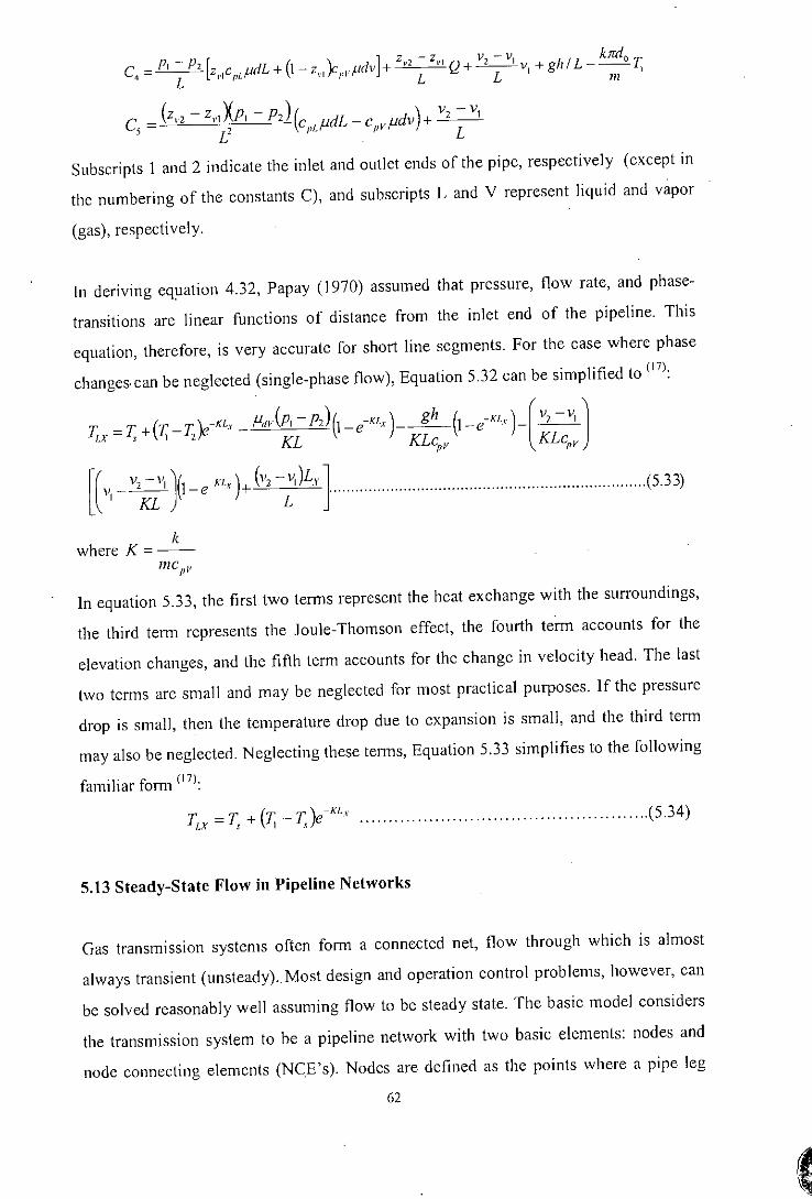
c,
c,
I'-P[ )c ]Z-Z v-v brd, 'z C fldL + (1 - Z .lldv +"' ,-,Q + _2__ ' V + gil / L - __ 0 TL l'I pI. 1'1 1,1" L Lim 1
(2" - 2" Xp, - p,) (c j1dL _ C j1dv) + V, - V,L2 pI. pV L
Subscripts 1 and 2 indicate the inlet and outlet ends of the pipe, respectively (except in
the numbering of the constants C), and subscripts L and V represent liquid and vapor
(gas), respectively_
In deriving equation 4.32, Papay (1970) assumed that pressure, flow rate, and phasc-
transitions are linear functions of distance from the inlet end of the pipeline. This
equation, therefore, is very accurate for short line segments. For the case where phase
changes. can be neglected (single-phase flow), Equation 5.32 can be simplified to (17!:
J;.x = T;+(1; - r,)e-KL, j1,IV(P,- P')(I_e-K1x )_~(I_e-KL, )_(1" -v, IKL KL~v KL~vj
l(v, - v';~")1- e-KL, )+ (v,-2' )L, }... (5.33)
Iewhere K=--
mcpv
In equation 5.33, the first two tenns represent the heat exchange with the surroundings,
the third ternl represents the Joule-Thomson effect, the fourth term accounts for the
elevation changes, and the fifth term accounts for the change in velocity head. The last
two terms are small and may be neglected for most practical purposes. If the pressure
drop is small, then the temperature drop due to expansion is small, and the third term
may also be neglected. Neglecting these terms, Equation 5.33 simplifies to the following
familiar fornl (17!:
T,v =T +(T.,-T)e-KL, •••..•.••.••....•••.•.••..•.•..••..•.••..•.••..•.• (5.34)
_,\ s S
5.13 Steady-State Flow in Pipeline Networks
Gas transmission systems often form a connected net, flow through which is almost
always transient (unsteady). Most design and operation control problems, however, can
be solved reasonably well assuming flow to be steady state. The basic model considers
the transmission system to be a pipeline network with two basic elements: nodes and
node connecting elements (NCE's). Nodes are defined as the points where a pipe leg
62
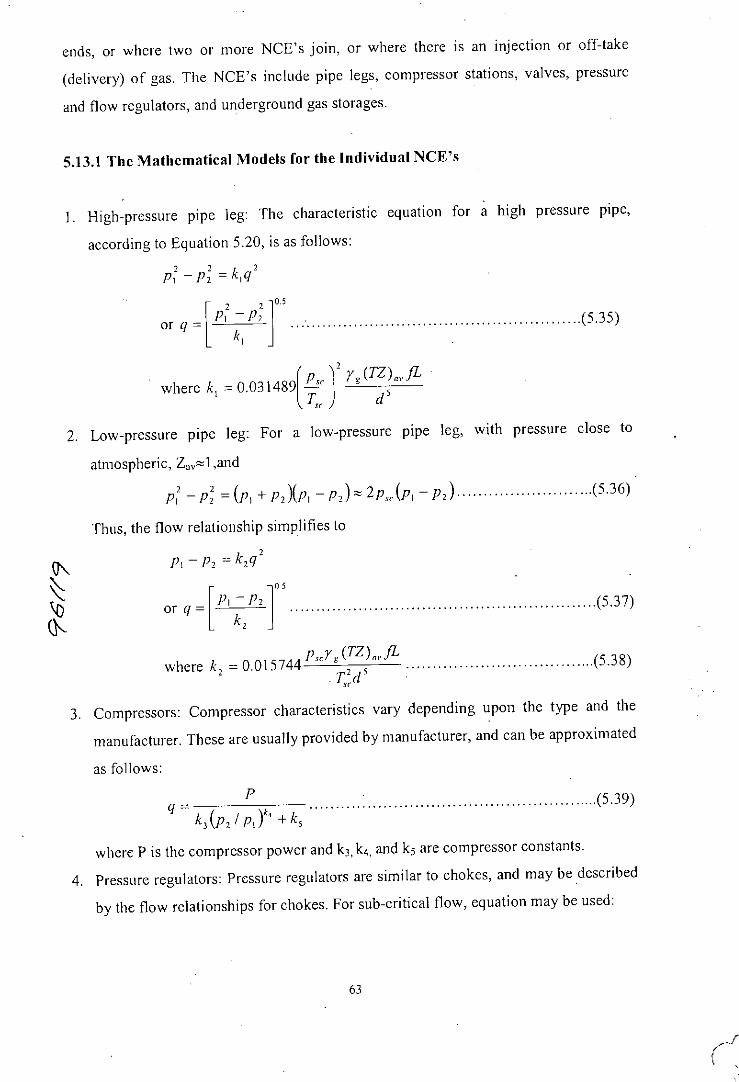
ends, or where two or more NCE's join, or where there is an injection or off-take
(delivery) of gas. The NCE's include pipe legs, compressor stations, valves, pressure
and flow regulators, and underground gas storages.
5.13.1 The Mathematical Models for the Individual NeE's
I. High-pressure pIpe leg: The characteristic equation for a high pressure pIpe,
according to Equation 5.20, is as follows:
2 2 k 'P, - P, = ,q
I' ,J0.5or q = (, I~P, (5.35)
2. Low-pressure pipe leg: For a low-pressure pipe leg, with pressure close to
atmospheric, Zav'"1,and
P,' - P~ =(PI + P,)(P, - p,)'" 2p,,(PI - p,) (5.36).
Thus, the flow relationship simplifies to2P, - P, = k,q
or q = lP, ;,P2r (5.37)
p"y g (TZ)"fLwhere k, = 0.015744 2 , •••••.•••••.•••••..••....•••...••••. (5.38)T"d'
3. Compressors: Compressor characteristics vary depending upon the type and the
manufacturer. These are usually provided by manufacturer, and can be approximated
as follows:p .
q = k](p, I p,)" +k, (5.39)
where P is the compressor power and kJ, k4, and ks are compressor constants.
4. Pressure regulators: Pressure regulators are similar to chokes, and may be described
by the flow relationships for chokes. For sub-critical flow, equation may be used:
63
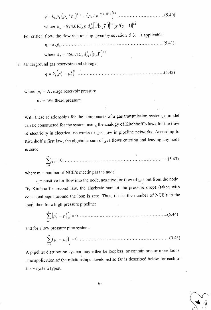
r( )" x ( )(X+')I X ]0.5q =k"p,t 1', II', - 1',11',. . (5.40)
where k6 = 974.6ICdp,d:JI/(rgd05[x/(X-I)r'
For critical flow, the flow relationship given by equation 5.31 is applicable:
q = k,p, (5.41)
where k, = 456.7ICdd:;, I(r gT, )05
5. Underground gas reservoirs and storage:
(, ,)".q = kg 1', - 1', (5.42)
where 1', = Average reservoir pressure
1', = Wellhead pressure
With these relationships for the components of a gas transmission system, a model
can be constructed for the system using the analogy of Kirchhoffs laws for the flow
of electricity in electrical networks to gas flow in pipeline networks. According to
Kirchhoffs first law, the algebraic sum of gas flows entering and leaving any node
IS zero:mLqi = 0 (5.43)
;=1
where m = number ofNCE's meeting at the node
q = positive for flow into the node, negative for flow of gas out from the node
By Kirchhoffs second law, the algebraic sum of the pressure drops (taken with
consistent signs around the loop is zero. Thus, if n is the number of NCE'sin the
loop, then for a high-pressure pipeline:
:t(1',' - p;)i = 0 (5.44);=1
and for a low pressure pipe system:
"L(I', - 1',) = 0 (5.45)i"l
A pipeline distribution system may either be loopless, or contain one or more loops.
The application of the relationships developed so far is described below for each of
these system types.
64
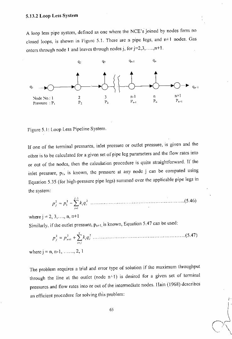
5.13.2 Loop Less System
A loop less pipe system, defined as one where the NeE's joined by nodes form no
closed loops, is shown in Figure 5.1. There are n pipe legs, and n+ I nodes. Gas
enters through node 1 and leaves through nodes j, for j=2,3, ..... ,n+ 1.
q, q"
q,
Node No.: ]Pressure : PI
2P,
3P,
n-]
Pn-lnP"
n+!Pn-t-l
Figure 5.1: Loop Less Pipeline System.
If one of the terminal pressures, inlet pressure or outlet pressure, is given and the
other is to be calculated for a given set of pipe leg parameters and the flow rates into
or out of the nodes, then the calculation procedure is quite straightforward. If the
inlet pressure, PI, is known, the pressure at any node j can be computed using
Equation 5.35 (for high-pressure pipe legs) summed over the applicable pipe legs in
the system:i-I
, ''''k 2Pi = P, - L. i'Ii;=1
. . .. . .. . . . . .. . . . . . . . .. . . . . . . . .. . . . . .. . . . . .. . .. . . . . .. . ... (5 .46)
wherej = 2, 3, .... , n, n+1
Similarly, if the outlet pressure, Pn+l, is known, Equation 5.47 can be used:
"P: = p,~"+ Lki'Ii' (5.47)i==j
wherej = n, n-I, ,2, I
The problem requires a trial and error type of solution if the maximum throughput
through the line at the outlet (node n+1) is desired for a given set of terminal
pressures and flow rates into or out of the intermediate nodes. Hain (1968) describes
an efficient procedure for solving this problem:
65
I',II
\
0,,'c;\ i \- \.

1. Guessing the maximum throughput of pipe leg 1, q~'). The superscript (1)
indicates that this is a first approximation.
2. Calculating the throughputs for individual pIpe legs, q~') usmg equation
5.46.
3. Using equation 5.47, calculate the outlet pressure for the system, (p~':,)4. If (p~':,)differs from the given outlet pressure- P'~+I by a value greater than
the prescribed tolerance, then correct the throughputs for the individual pipe
legs detemlined in step 2 using:
q?) = q~')+ f\.q (5.48)
where f\.q
5. Repeating steps 3 and 4 until convergence within a specified tolerance is
reached.
In step 4, the correction f\.q becomes more complex for flow systems with a greater
variety of NCE's. Hain (1968) gives the following correction for a line containing a
compressor station:
f\.q = _I(p~'!,)'- P,~",II,: (5.49)
[(p~), - (PI'),]; q, +L),q?)where (PI),.' (p,),. = compressor intake and discharge pressures, respectively, psia.
5.13.3 Looped Systems (17)
There are two types of looped pipe systems: single-loop (Figure 4.2), and multiple-loop
(Figure 5.3). Cross (1936) gave the first solution for low-pressure looped systems,
which was later extended to high-pressure systems (Hain, 1968).
66
r:

5.13.3.1 Single-Loop System
q,
Tq,
Figure 5.2: Single Looped Systems
B
A
Figure 5.3: Multiple Looped System
c
D
67
................ ~
......~
.......~
................••

The problem requires a trial and error solution scheme. An initial value for the flow rate
in pipe leg I is assumed. If this assumed value, q;'), differs from the actual throughput
by !'o.q, then by the node law of Equation 5.44 or 5.48 for steady-state flow (17.21):
I k;(q~i) + !'o.qM) + !'o.ql= 0 (5.50)i=l
where n = number of pipe legs in the single-loop system.
Solving equation 5.50 for !'o.q, and assuming that !'o.q« q, we get:
- Ik,lq!')ll)!'o.q - '='" (5.51)
22),jq!')\1=1
The gas throughputs for the next iteration, q~2) , are computed as before (Equation 5.48):
q~2) = q!') +!'o.q (5.52)
This procedure is repeated until for iteration k, !'o.qis less than or equal to a specified
tolerance. After this successful k-th iteration, the node pressures can be calculated using
the relationship (Equation 5.46) for a high-pressure network:i-i .
2 2" I (k)I (k) .Pi = P, - ~k, q, q, (5.53)i=l
for j= 2, 3, .... , n, n+ 1
where ki for pipe legs are calculated using Equation 5.35 for high-pressure lines. For a
low-pressure network, k, for pipe legs are calculated using Equation 5.37, and the node
pressures are computed using Equation 5.54:
P, = P, - 2),lq)k1Iq!!) (5.54)
for j= 2,3, .... , n, n+1
68

5.13.3.2 Multiple-Loop System
Stoner (1969, 1972) has presented an effected method for handling looped networks
with all kinds ofNCE's. In this method, the equation of continuity is used to express the
flow at each node in the system. The solution to the system of equations is complex, but
the method offers the ability to compute any set of unknowns. It thus overcomes the
limitation of the Cross method that can only be used to generate throughput or pressure
solutions. Illustration for Stoner's method is shown in Figure 5.4.
Figure 5.4: Illustration for Stoner's Method (17).
For any node j, the continuity equation (Equation 5.43) express the fact that the sum of
the inflows and outflows at the node is zero:
"Fj
. =" q (5.55)~ I,)
;=1
where q i,j is the flow from node i to node j, flows into the node are considered positive,
flows out of the node are negative. Fj thus represents the flow imbalance at the node and
will be equal to zero when the system is in balance, For example, consider node 2 that
receives gas from gas from underground storage (1,2) and pipe leg (10,2), and delivers
gas to compressor intake (3,2), and consumer supply attached directly to node 2.
Equation 5,55 for node 2 can now be written as:
F2= ql.2 - q),2 + QIO,2 - q, = 0 (5.56)
69

With the substitution of the appropriate NeE equations (from Equations 5.35 through
5.48), Equation 5.56 becomes:
( ) ( 2 2)" P,-4 (p,20 - p~t~ (557)F, ~ k p, -p S, - . +~~~S ,-q ~o .~ l\ 1,2 _ I I,~ k ( / )" k (k )0,5 l().~ 2
.1 P4 P.I + 5 \ 0.2
where S'j is the sign term that accounts for the flow direction:
S'.i = sigll(p, - Pi)
= + 1 for Pi 2:Pi
= -1 for Pi< Pi
Similar equations are written for all the other nodes in the system. Each of the node
continuity equations, such as Equation 5.57, can be expressed as follows:
FJx"x2,x" ,xJ = 0, for j=l, 2, 3, , n (5.58)
This non-linear system of equations can be solved using various iterative techniques on
a computer. Stoner (between 1969 to 1972) used the most popular solution method:
Newton-Raphson iteration. The values of the unknowns are computed repeatedly, until
the values from any two successive steps converge. The values of any unknown at the
(k+ 1) th iteration is computed as follows:
X~k+l)= X!k) + ,',x)'+') (5.59)
" ofwhere ",,_.l,',x. = -F forj. = 1 2 , nL...~ 1.1' "i=1 uXi
wherc the derivatives &F/&x, are obtained by differentiating the node continuity
equations. The method reqUlres an initial estimate for each of the unknowns, XiO
Generally, good initial guesses are required to achieve satisfactory convergence. A
standard mathcmatical technique for improving and accelerating convergence is to
introduce an accelerating factor, (X,. in the correction (Equation 5.59), as done by Stoner
in 1969:
xi"') = x!') + ,',xi'+I)a, (5.60)
where (x, is computed using the t.Xi for the current and previous steps. Stoner (1969)
proposed the following scheme for obtaining (Xi
Let A, = ,',x!'+I) / ,',x!'). For the first two iterations, where divergence is most likely tooccur, an (Xi = 0.5 is best to use in order to ensure convergence. In subsequent steps, the
70

OJ = O.SIAjl
OJ = 1.0 - O.SIAj IOJ = 1.0 + O.SIAjl
For-1<A1<1,
value of (Xi is determined as below for every other step; for the steps in between, (Xi = 1.0
is used:
For Aj ~ -1,
For Aj 2: 1, ° =3,
Stoner obtained these specifications for (Xi by experimenting with the mathematical
model on a computer. Naturally, these are empirical, system-dependent values, and the
user may have to do some experimentation to obtain similar or better schemes for the
acceleration factor (Xi applicable to the system.
71

Chapter 6
SIMULATION RESULTS
6.1 Introduction
The major part of the future energy demand would be met from natural gas and it is
estimated that gas demand would reach about 1450 MMSCD (average) and 1700
MMSCFD (maximum) by 2005 and 1900 MMSCFD (avg.) and 2250 MMSCFD
(max.)(4) by 2010. In this Chapter,. high-pressure transmission network has been
simulated and pressure at different sources, sinks and manifolds are matched with the
existing conditions. The existing pipeline capacity is analyzed and the level of capacity
utilization is examined. Then different cases have been studied for future prediction.
6.2 Demand-supply Scenario of High-pressure Gas Transmission Lines of
Bangladesh Using Current Data
The transmission pipeline network compnses of high-pressure trunk gas pipelines,
which operate at a pressure greater than 900 psig. Gas production in 24 hours from 12-,
July-OO to 13-July-00 was 931 MMSCFD. Out of this, Jalabad franchise area (.lFA),
Titas franchise area (TFA), Bakhrabad franchise area (BFA) and Westem region
franchise area (WFA) consumed 54, 621, 241 and 15 MMSCFD of gas, respectively.
Figure 6.1 shows the present network system. Description of the present network IS
given below.
6.2.1 North South Gas Transmission Pipeline (N-S line)
The North South pipelines was built under the Projcct Implementation Unit (PIU) of
Petrobangla which was then transferred to the Gas Transmission Company Limited
(GTCL), now in charge of operating this pipeline. World Bank financed this project.
The North South pipeline was commissioned in May 1992 but put in operation in
September 1993. It is a 175 km pipelinc of 24" diameter, made of OS' wall thickness
API5L grade X56 line pipes. Its origin is at Kailashtilla manifold station and termination
point is at Ashugonj metcring station where metering, regulating and fractionation
facilities are in place. It was built by SAIPEM (Itally). It transports gas from Kailashtilla
72

_L.
P: 106B Psig
Tltel$GF: 303.2 mmscfld
Sheh;PP: 36.61 mrnsc11d
N106: 5.00 ntnsc1~
Fef'ilP: 0.00 mmscfldRashidGF: 70.62 mm,d/d
4)HOF1: 187.9 mmscl/d
KTL234 6B.09 mm,d/d r,;}P: 1090 p,ig ~~odGF: 1092 Psig
F: 82.54 mmscf/d
(\)
Menifold
•TN1eK8I:ihata
r ,j ;'rl"
/
G ZiOFF:0.0~11d
Sal . APS: 1da. 15.12 rrmsd/d 00,99 mmscffd
. CtgCity:241.2 mmscf/d;: ," !F .-.-&...-o-.O-.~O-.e-_._e-_~.
Bokhro' K"Bopur eto L••••••m Ford J42 _OllO. BEWobP: 1075 Psig
",,",c'"D8Ulot#
1oIegt-naPP: 0.00 """did
D~1~e
73
•10 TN3
~
eg,BeloboOF 17.14
16.31 mmsd/d BekhraGF
8D hn~ 34.43 mrmlcl/d
MenthOl'~
Han?P: 29.BFi m'ffiicf/d
10
p
T8~T'.Jrsbo*
Dhanua
Sl'*JdPS 14.62 rrrnscfJd
Psigo
o
~ OO~"'~ c1ld~ur: 3. l\tnenPP:14.~e... NelKono: 200 """''lour
N16
JB1JB2
P 1006 Plig
~Jo
P: 1
B8ari:
Nob
Figure 6.1: High Pressure Gas Transmission Lines of Bangladesh simulated by Using Current Data
()
gas field, J alalabad gas field and Beanibazar gas field ta the inlet .of Narth Sauth
pipeline (Kailashtilla manifald statian). Gas alsa carnes from Rashidpur gas field and
Habiganj gas field ta the Narth-Sauth line at Rashidpur manifald statian and Habiganj
manifald statian respectively. There is na bulk cansumer from Narth-Sauth line except
90 MW Fenchuganj pawer plant, which cansume gas from Fenchuganj manifald
statian. The maximum allawable .operating pressure .of the N-S pipeline is 1135 psig, its
maximum inlet pressure 1090 psig. And the narmal pressure at Ashuganj is 850 psig.
The capacity afthis line is 385 MMSCFD.
6.2.2 Bakhrabad to Chittagong Gas Transmission'Pipeline (B-C line)
B-C line is a 174 km lang, 24" diameter pipeline. Its inlet paint is at Bakhrabad
manifald statian and .outlet paint is at Faujdarhat city gate statian. There is na bulk
cansumer al.ong this line.>Its capacity is 350 MMSCFD. The pressure at Bakhrabad
manifald statian is between 850 and 900 psig and with the maximum flaw rate .of 170
MMSCFD at Bakhrabad. The pressure dr.op is abaut 100 psig ta ga ta Chittagang. The
gas at Chittagang is distributed in a 350 psig ring main around the city. Mast cansumers
there are bulk c.onsumers, pawer plants .or fertilizer fact.ories. The damestic cansumptian
is .only 4% .of the tatal. The delivery pressure t.o all pawer and fertilizer plants is 350
psig except the delivery pressure ta KAFCO fertilizer plant in Chittagang, which is .only
120 psig.
B-C line is unfartunately limited at ANSI 400. This is inc.onvenient because it limits the
pipeline MAOP ta 960 psig but alsa because ANSI 400 valves and fittings are nat easily
f.ound an the market and can nat be exchanged with ather gas transmissian campanies
which are using ANSI 600 equipment. A cathadic protectian is applied an the pipeline
with a negative valtage .of at least 0.85 V between the pipe and a saturated caper- caper
sulfate reference electrode, which is satisfactary.
74

6.2.3 Ashugonj to Bakhrabad Gas Transmission Pipeline (A-B line)
To create stability in transmission system of Bakhrabad Franchise Area, A-B line is
constructed. It has also benefited from the physical integration of the three systems, such
as JFA, TFA, and BFA. GTCL is responsible for the operation of the A-B line. This
pipeline is 59 km long, 30" diameter, made of APIX52 line pipes with a MAOP of 1000
psig and ANSI 600 ancillaries. A 10m wide right of way was acquired with a IS m
wide working area during construction. This line delivers gas from Ashugonj metering
station to Bakhrabad manifold station. There is no bulk consumer from this line. Its
capacity is 500 MMSCFD. Mc Connel-Dowel of Australia constructed this line.
6.2.4 Bakhrabad to Demra Gas Transmission Pipeline (B-D line)
The gas flowing from Ashugonj to Bakhrabad will supplement the short supply from the
Bakhrabad gas field to the Chittagong area. To create stability in the transmission
system an idle pipeline was constructed to flow gas from Bakhrabad to Demra. It is a 68
km long, 20" diameter pipeline. Its origin is at Bakhrabad manifold station and
termination point is at Demra City Gate Station. Haripur power plant receives gas from
Dewanbag manifold station of Bakhrabad-Demra line. Its capacity is 250 MMSCFD.
The pressure of Bakhrabad-Demra line is smaller than the other transmission lines due
to the pressure problem of Bakhrabad gas fields. There are valves in inlet and outlet of
Bakhrabad-Demra line for controlling flow as well as pressure in Bakhrabad-Demra
line. There is also a by pass line from Bakhrabad manifold station to the point where
Bakhrabad gas field connects with the B-D line. A pressure regulator is connected to
this by pass line to regulate pressure according to the pressure of Bakhrabad gas field.
Even though, Demra City gate station accepts gas from Bakhrabad-Demra line by
controlling pressure (using pressure regulator) ofDemra city gate station. Spie-Capag of
France completed sub-surface drilling over Meghna River (4700 feet) by Directional
Drilling Method.
6.2.5 Ashugonj to Elenga Gas Transmission Pipeline (A-E line)
A-E line, which is known as Brahmaputtra Basin line, is a 124 km, 24" diameter
pipeline. Its inlet point is at Ashugonj metering station and outlet point is at Elenga
75
manifold station. It delivers gas to Kishoregonj from Monohordi manifold station;
Netrokona, Mymenshing power plant from Dhanua manifold station; Sherpur, Jamuna
fertilizer factory, Jamalpur from Elenga manifold station. Its capacity is 340 MMSCFD.
A-E.line was commissioned in 1991. Spie Capag of France constructed Titas-Elenga
Transmission lines. Both Elenga-Tarakandi line (43 km, 12" aD) and Dhanua-
Mymenshing line (56 km, 12" aD) were commissioned in 1991. Both Monohordi-
Kishoregonj line (35 km, 4" aD) and Tarakandi-Sherpur line (47 km. 8"/6" aD) were
commissioned in 1993. 40 km, 8"/6" Mymenshing-Netrokona line was also
commissioned in 1993.
6.2.6 Titas-Narsingdi-Demra Gas Transmission Pipeline (T-D line)
It is an 81 km long, 14" diameter pipeline. Its capacity is 175 MMSCFD. There are two
bulk consumers (Ashugonj power station and Zia fertilizer factory) from this line. Its
origin is at Titas gas field and termination point is at Demra city gate station. This line is
commissioned in 1968. Mis Society Des Grands Travaux De Marseille (GTH) of France
constructs this line.
6.2.7 Titas-Narsingdi-Joydevpnr Gas Transmission Pipeline (T-J line)
It is an 82.81 km (46.3Ikm + 36.50km) long, 16"/14" diameter pipeline. Its capacity is
265/220 MMSCFD. Its origin is at Titas gas field and termination point is at Narshindil
Joydevpur city gate station. Both Titas-Narshindi line (46.31 km, 16" aD) and
Narshindi-Joydevpur line (36 km, 14" aD) were commissioned in 1985. There are two
lines between Narshindi city gate station to Ghorasal manifold station. One line is 12 km
long, 14" diameter and other line is 12 km long, 16" diameter which is parallel to each
other. 12 km, 14" aD Narshingdi-Ghorasalline was commissioned in 1970 and 12 km,
16" aD Narshingdi-Ghorasal line was commissioned in 1999. Ghorasal manifold
station is the focal manifold of this line because two fertilizers and one power station
receive gas from this manifold. The capacity of Narshingdi to Ghorasal line is 370
MMSCFD. A group of companies are constructed T-J line. The name of the companies
are given below:
i) Maxwell Engineering Works Ltd.
ii) Probash Prokaushali

iii) Royal Utilization Services (Pvt.) Ltd.
iv) Business King
v) Shamsuddin Miah and Associates Ltd.
vi) Dawn Construction and Co. Ltd.
6.2.8 Monohordi-Narsingdi-Shiddhirgonj Gas Transmission Pipeline (M-S line)
It is a 67 km long, 20" diameter pipeline. Its starting point is Monohordi manifold
station and ending is Shiddhirgonj District Regulating station. Shiddhirgonj power
station consumes gas from this line. This line is inter connected to 14" Narshingdi-
Demra line. Monohordi-Narshingdi line and Narshingdi-Shiddirgonj line were
commissioned in 1997 and 1999 respectively.
6.2.9 Western Region Gas Transmission Line
It is 70 km long, 24"/30"/24"/20" diameter pipe line. Its ongm is Elenga manifold
station and tennination point is Baghabari station. Baghabari power station consumes
gas from this line.
6.2.1 0 Network Analysis
The network is analyzed by assuming 1092 psig pressure at Ialalabad gas field. The
simulated flow rate of Ialalabad gas field is 82.54 MMSCFD that is nearly accurate to
the original value (82.66 MMSCFD). Hence the simulation is correct. The simulated
results and pressure drop along the transmission lines are tabulated in Appendix 1. The
capacity of the North-South pipeline is 335 MMSCFD.
The variations of pressure and flow rate with the length are shown in figure 6.2 and 6.3.
NOffilally, as a rule of thumb 1 psig pressure drop occurs for 15-km length. From figure
6.2, it is clear that the pressure in North-South line is gradually decreased from 1090
psig to 1077 psig (pressure drop 13 psig) for 174 km. Velocity of gas in Bakhrabad-
Demra line (3.36 million fUhr) is greater than the Bakhrabad-Chittagong line (1.59
million fl/hr). Hence the pressure drop in Bakhrabad-Demra line is greater than the
Bakhrabad-Chittagong line.
77

I-+--N-S line-D- B-C line
B-D lineA-E line
200150100Length, Km
50o1065
1090
1085OJ i'iii I0- 1080 IQ)
I I~:J({) 1075 ''\"~~J::l-_ !(() --~--nf$___Q)~ I '0Q.. 1070
Figure 6.2: Variation of Pressure along the Major Gas Transmission Lines.
I
! ! II ' I
I : I, I
! - I !, I I~ • L_ . I I
I ; I, I I, , ,
400350o
b 300~ 250~ 200Q)~~ 150~ 100
LL50
oo 50 100
Length, Km
150
1I
I
200
-+- N-S line--/lO-- B-C line
B-D lineA-E line
Figure 6.3: Change ofFlowrate along the Major Gas Transmission Lines.
78

Figure 6.3 shows the variation of flow rate along the transmission lines. In North-South
line, first jump of flow rate occurs due to the addition of 70.62 MMSCFD at Rashidpur.
The second jump of flow rate occurs due to the addition of 132.24 MMSCFD at
Habigonj from Habigonj Gas Field. In Bakhrabad-Chittagong line, jump of flow rate
occurs due to the addition of 119.8 MMSCFD of gas at Faujdarhat manifold station
from Sangu gas field. In A-E line, 1st jump of flow rate occurs due to the addition of
83.11 MMSCFD gas at Daulatkandi from Daulot# (Manifold station on 16" Titas-
Narshingdi line). At Monohordi point, a sharp decrease in flow rate is observed due to
158.8 MMSCFD of gas is delivered to Narshindi manifold station and Kishoregonj area
from this point.
On July 12, 2000, the inlet and outlet pressures of North-South line were 1090 psig and
915 psig, respectively; but the simulated pressures in this line were 1090 psig and Ion
psig respectively. Therefore, a 17.6 % error in pressure was observed at Ashugonj
metering station. Demra, Chittagong, Bakhrabad, Elenga, Narshingdi, Ghorasal and
other important points also showed unacceptable pressure differences.
Variation of liquid holdup along the North-South pipeline is shown in Figure 6.4. At
Kailashtilla manifold station, the liquid holdup is 52.7% only. This value is become 53.9
% up to Rashidpur manifold station. After Rashidpur manifold station, liquid holdup is
decreased due to the addition of dry gas from Rashidpur gas field at Rashidpur manifold
station. At Habigonj manifold station, liquid holdup is 44.8% only. After this point, this
value decreases again due to the addition of dry gas from Habigonj gas field at Habigonj
manifolld station. At Ashugonj metering station, liquid holdup increases and becomes
25.9 % due to pressure drop.
79

60
50;,Roci 40:::l-0
o 30I-0
'S 200-:.::J
10
, ,: --+-- N-S line i
oo 50 100
Length, km
150 200
Figure 6.4: Variation of Liquid Holdup along the North-South Pipeline
If the same simulation is revised with the known pressure at Kailashtil1a manifold
station (1090 psig) and Ashugonj metering station (915 psi g); the simulated pressure at
other manifold station nearly matches with the measured data. Figure 6.5 shows the
present scenario. Good pressure match is observed at different nodes and delivery
points, which is shown in Table 6.1. The percentage of error at different nodes and
manifolds are very low (Table 6.1). Figure 6.6 shows the comparison of calculated
pressure to the measured pressure of North-South line. There is almost negligible
pressure error is observed at North-South line. But from Figure 6.7, it is observed that
the pressure drop in Bakhrabad-Demra line is greater than the Bakhrabad-Chittagong
line. Since the velocity of gas in Bakhrabad-Del11ra line is greater than the Bakhrabad-
Chittagong line, therefore, the pressure drop in Bakhrabad-Demra line is greater than the
Bakhrabad-Chittagong line. Even through, the pressure drop in North-South line is 174
psig. A significant pressure drop and flow constraints is also observed at Ashugonj-
Bakhrabad line and Narshindi-Demra line. Therefore, it is required to find out the reason
of the above situation.
80

HGf: 18790mmscf/d
TitasGF: 303 mmscl/d
FenPP: O.OOmmscf/d
ShahjiPP: 36.61 mmscf/d
N106: 5.00 mmscf/d
Barab Fa~darCtgCity: 750.00 psig
MSharai
lani10ld
J42
TN1
Kalihata
8.[ line
Feni
KTL1~KTL234f ':12 604 68 08£ P 1090 PStgmmscf/d mmscf/d JalaGE.
~ /P1090P"g
N61 - _...@KTdl~1\1111 ~.,... 88azer 0 00 mmscl/d
ZiaFF: 0,00 m~f~i/d100.99 mmscf/d
Laksham
N108: 916.00 psig
Sylhet: 17.28 mmscf/d
.".-8 line
Bakhra
P: 891.17 Psig KuBapur SIJreMegilePP
A.c i:n",
B.D line
BeleboGF: 16.31 mmscf/dMeghnaG
~fl
T
Dhanua
N107: 5.00 mmscf/d
ShiddPS: 14.62 m~~~rrd 29.86 mmscf/d MegPP: 0.00 mmscf/d
P: 864.98 Psig
DGhoraFF: 43.20 mmsc&Ro~aFF
~
~ ~mmS1U~enpp ~ ~N98: 4.00 mmscfld Ja~pur ~ LX NetKona:
j ~menDMymen: 2.00.mmscf fJ
P: 862.53 E'.,.r,g,~.Nr:,binePsig
NoIlka JB2
BBeri: 13.19 mmscf/d
DGulshen: 52.00 mmscfll
DJDevpur: 6.00 mmsc1fd
DemriDDemre: 87.00 P: 750.01
mmscf/d Psig
SanguOF: 119.8 mmscl/d
8o
Figure 6.5: Demand-supply Scenario of High-pressure gas transmission lines of Bangladesh modified by known pressure at Ashugonj.
81

I~---.._.--.---..
--+- Calculated-_ Measured
200
. ~~---~~---
50 100 150
Length, Km
o
.Ql 1100C/)
0.. 1050
~ 1000::lC/)C/) 950~
0.. 900
Figure 6.6: Calculated and Measured Pressure along the N-S Line.
--+- N-S line--B-C line
I B-D line_....~~E line
-----.----1
~::lC/)C/)
~0..
11501100 - -------.-~ .. --._._.--.~.--.~._~-~.~--~--._-~-~--- ..
1050
.~ 1000c.
950900 ,1--
850 ---.- - - - - .. -
800 -~----.-.----
750
700o 50 100
Length,Km
150 200
Figure 6.7: Variation of Pressure along the Major Gas Transmission Lines after
Modification
82

Table 6.1: Comparison of Simulated Pressure to the Measured Pressure
Node/ Delivery Point Measured Calculated %Pressure (psig) Pressure (Psig) Error
APS 860 873.11 0.02GhorasalPP 685 655.55 0.04HaripurPP 700 761.61 0.09RPCL(PP) 830 855.71 0.03GhorasalFF 704 793.82 0.13Bakhrabad 867.3 891.17 0.03Ashugonj 915.81 915.79 0.00Demra 710 750.01 0.06Chittagonj 712.5 700 0.02Kailashtilla 1090.74 1090 0.00Rashidpur 1046.64 1035 0.01Habigonj 1020.41 1005 0.02
The reasons of flow constraints are given below:
i) Due to the condensate accumulation in transmission lines, the effective
diameter of the lines may get reduccd and flow constraint may arise.
ii) Due to the corrosion of pipe, the roughness of the pipe may increase.
Hence pressure drop through the line will increase.
iii) Un-authorized delivery line (which is common problem in Bangladesh)
can exist in the transmission system. Hence pressure drop may arise.
Variations between simulated results and measured results might be due
to the system loss in transmission system. During 12-lul-00 to 13-lul-00,
the production of gas was 931 MMSCFD but consumption was only 905
MMSCFD. Therefore, 26 MMSCFD of gas are lost during transmission
and distribution system.
iv) During the simulation pressure losses due to valves and fittings are over
looked.
v) There are two-flow controllers, one the Ashugonj to Elenga line and the
other on the Ashugonj to Bakhrabad line that are over looked during
simulation due to the Software limitations. The flow controllers are used
to control flow of A-B line and A-E line. The diameter of A-B line is
83
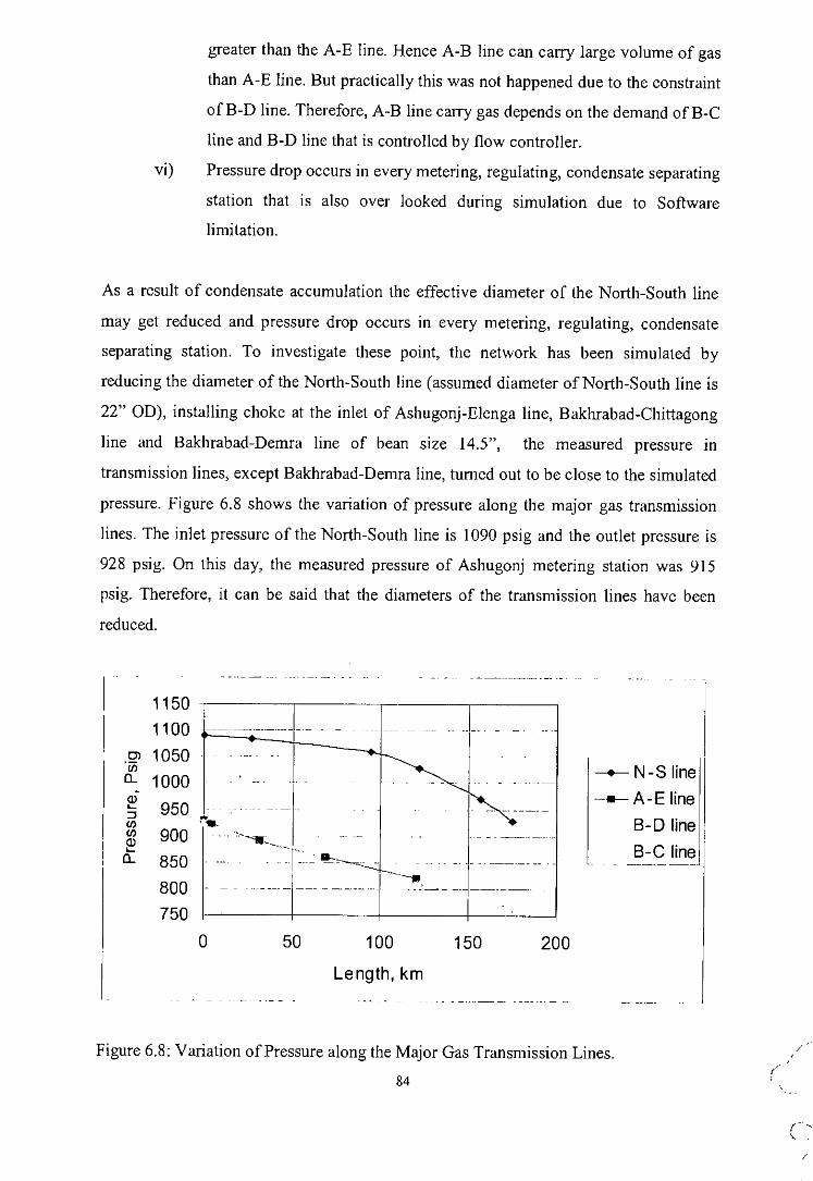
greater than the A-E line. Hence A-B line can carry large volume of gas
than A-E line. But practically this was not happened due to the constraint
ofB-D line. Therefore, A-B line carry gas depends on the demand ofB-C
line and B-D line that is controlled by flow controller.
vi) Pressure drop occurs in every metering, regulating, condensate separating
station that is also over looked during simulation due to Software
limitation.
As a result of condensate accumulation the effective diameter of the North-South line
may get reduced and pressure drop occurs in every metering, regulating, condensate
separating station. To investigate these point, the network has been simulated by
reducing the diameter of the North-South line (assumed diameter of North-South line is
22" OD), installing choke at the inlet of Ashugonj-Elenga line, Bakhrabad-Chittagong
line and Bakhrabad-Demra line of bean size 14.5", the measured pressure in
transmission lines, except Bakhrabad-Demra line, turned out to be close to the simulated
pressure. Figure 6.8 shows the variation of pressure along the major gas transmission
lines. The inlet pressure of the North-South line is 1090 psig and the outlet pressure is
928 psig. On this day, the measured pressure of Ashugonj metering station was 915
psig. Therefore, it can be said that the diameters of the transmission lines have been
reduced.
11501100
.gJ 1050(/)
D.. 1000
~ 950:J(/)
(/) 900~D.. 850
800
750
.w.... - ..,.....--.:.-.
o 50 100
Length, km
150 200
-+- N-S line
--A-E line
B-D line
B-C line
Figure 6.8: Variation of Pressure along the Major Gas Transmission Lines.
84

The outlet pressure of the Bakhrabad-Demra line is 784 psig that is larger than the
measured pressure. The measured pressure of Bakhrabad-Demra line varies from 550
psig to 600 psig that depend on the pressure of Bakhrabad gas field. The measured
pressure .of Bakhrabad gas field was 600 psig. In the next simulation, attempts were
made to match pressure at Bakhrabad gas field.
6.3 Modification of Network by Using Known Pressure at Bakhrabad Gas Field
From the previous study, it is clear that the pressure at Bakhrabad gas field is 891 psig.
But it is impossible for this field to produce 35 MMSCFD at this pressure. Current
producing pressure of this field is 600 psig only. At present, Bakhrabad gas field is
connected to the network system by reducing the pressure of Bakhrabad-Demra line. To
reduce pre~sure of Bakhrabad-Demra line, two valves and pressure regulator are used
which are described before.
Currently Bakhrabad-Demra line is the focal line of the transmission lines, which is
treated as an idle line, which means that the volume it transports is much lower than its
capacity. Bakhrabad-Demra line transport gas to Demra city gate station and Haripur
power station. But pressure in Bakhrabad-Demra line is lower than the Demra city gate
station. Therefore, it is facing serious problems to transport gas parallel to the other
transmission lines. Low pressure at the Bakhrabad gas field has created this problem
because the field producil}g pressure is 600 psig. It is apprehended that if production of
Bakhrabad gas field is stopped, the well would die due to accumulation of sand and
water. There are valves in inlet and outlet of Bakhrabad-Demra line for controlling flow
as well as pressure in Bakhrabad-Demra line. There is also a by pass line from
Bakhrabad manifold station to the point where Bakhrabad gas field connects with the B-
D line. A pressure regulator is connected to this by pass line to regulate pressure
according to the pressure of Bakhrabad gas field. Even though, Demra City gate station
accepts gas from Bakhrabad-Demra line by controlling pressure of Demra city gate
station using pressure regulator. When Demra city gate station accept gas from~,
Bakhrabad-Demra line, delivery pressure from Demra City gate station decreases
drastically. The present simulation (Figure 6.9) is simulated by reducing the diameter of
85r-'-
.~-""(~-e,
/

North-South line, taking a separator at Ashugonj, installing a choke of bean size OS' in
the inlet of Bakhrabad-Demra line and blocking reverse flow from Demra city gate
station. Assuming 625 psig pressure at Bakhrabad gas field, the scenario is simulated.
The calculated flow rate of this field is 34.32 MMSCFD that is equal to the delivered
flow rate, 34.43 MMSCFD. The simulated results are shown in Appendix 3.
The variation of pressure with length are given in Figure 6.10. The outlet pressure of
North-South line is 917 psig that is close to measured pressure at Ashugonj (915 psig).
The measured pressure of Bakhrabad-Demra line varies from 550 psig to 600 psig that
depend on the pressure of Bakhrabad gas field. After simulation, the calculated pressure
along this line varies from 907 psig to 619 psig. Figure 6.11 shows the variation of flow
rate along major transmission lines modified by using known pressure (625 psig) at
Bakhrabad gas field. After Dewanbag manifold station, the flow rate of Bakhrabad-
Demra line is reduced and become zero because the outlet pressure of Bakhrabad-
Demra line is smaller than the Demra city gate station.
Effect of separator at the end of North-South line is shown in Figure 6.12. At
Kailashtilla manifold station, the liquid holdup is 40% only. This value is become 41.4
% up to Rashidpur manifold station. After Rashidpur manifold station, liquid holdup
decreases due to the addition of dry gas from Rashidpur gas field at Rashidpur manifold
station. At Habigonj manifold station, liquid holdup is 32.6% only. After this point, this
value decreases again due to the addition of dry gas from Habigonj gas field to Habigonj
manifolld station. At Ashugonj metering station, liquid holdup decreases and becomes
0.05 % due to separation of liquid from gas by using 90% efficient separator.
86
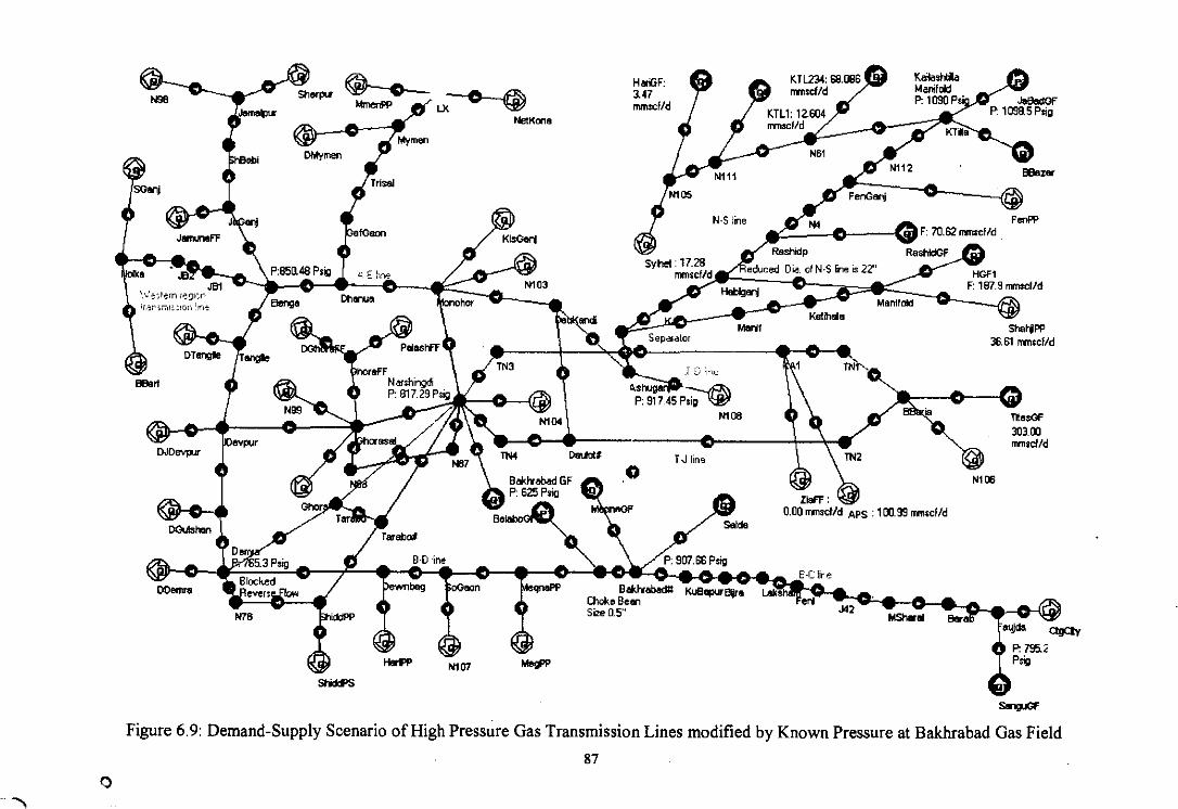
~da QgCIy
P: 795.2P,;g
Tlt• .oF303.00rrrn,cfld
FenPP
ShotjlP!'36.61 rrrnocfld
Nl06
ea.,
F: 70.62 fIlIllOcfld
_ ..
: 100.99 fIlIllOcfld
FenGanj
.142
E-Cnre
Manifold
Manlf
HalJigan]
Rashidp
educed Die. of N.S line is 22"
KatihEia
N.S line
T [i :I'-,'~
T.J line
Separator
Sylhel : 17.28rml$cf/d
HOliiF:3.47"""",lid
o
8""lYobadlI KuB"""'S-". L.I"il_'~enI'Choke Be8"lSize 0.5"
Me!1'PNl07
B.D fine
'ewnbog
-
~LX~KOO.
ShId'S
.e'JB1
\'.':;,!ern ,eQK,r,~,.~r';;r",I~_:iQt., lin",
N98
•
'SOMj
SnJuGf'
Figure 6.9: Demand-Supply Scenario of High Pressure Gas Transmission Lines modified by Known Pressure at Bakhrabad Gas Field
87
."Q

1200 -
1100----+-N-S line--A-E line
B-D lineB-C line
50 100 150 200
Length, km
Figure 6.10: Variation of Pressure along Major Transmission Lines modified by Using
Known Pressure atEakhrabad Gas Field
-+-N-S line--A-E line
B-D lineB-C line
20015010050
400o 350~ 300(fJ:2 250 -:2. 2002~ 150
~ 1~~ t=~~=----t=-----~-~-~-~- ~--~-=-----ol---~-o
Length, km-- -- ------------_._--------_.--- -~----.-.------_._--_.- ---~ --~
Known Pressure at Bakhrabad Gas Field
, \Figure 6.11: Variation of Flow Rate along Major Transmission Lines mod:ified-by Using
'l "
\ ''"''~
, ,'. ' n'- --'
88

45 .40. -~----- ._- ...-..- ..
?f2. 35 .---~-.- ...ci 30::J-0 25aI 20 -.-~--.._..-0.S 15 .CT::i 10--5.-----o
l. 1
-+- N-S line~- --------- --- -
o 50 100Length, km
150 200
Figure 6.12: Effect of Separator at the End of North-South Line
89 i,

6.4 Modification of Network by Setting up a Compressor Station at Bakhrabad
Gas Field
The pressure of Bakhrabad gas field is decreasing day by day. Current producing
pressure of this field is 600 psig (year 2000). Bakhrabad-Demra line accepts gas from
Bakhrabad manifold station by reducing and regulating pressure of this line. This is
possible by setting valves at the inlet and out let of Bakhrabad-Demra line. There is also
a by pass line from Bakhrabad manifold station to the point where Bakhrabad gas field
connects with the B-D line. A pressure regulator is connected to this by pass line to
regulate pressure according to the pressure of Bakhrabad gas field. This special
arrangement is taken only for accepting gas from Bakhrabad gas field. At Demra city
gate station, the pressure is regulated according to inlet pressure with pressure-regulator.
To connect Bakhrabad gas field with the transmission system without reducing the
pressure of B-D line, a compressor station need to set up at Bakhrabad gas field. To
investigate this point, setting up a compressor (700 hp, 70% efficiency) at Bakhrabad
gas field simulates the scenario (Figure 6.13). The simulated results are shown in
Appendix 4.
The variation of pressure and flowrate with length are given in Figure 6.14 and 6.15.
The inlet pressure to the N-S pipeline is 1090 psig. If a 70 % efficient compressor of
700 hp is set up at Bakhrabad, the pressure increase to 846 psig which is close to the
Bakhrabad-Demra transmission line. Figure 6.16 shows the effect on transmission
system after setting up a compressor at Bakhrabad gas field. Therefore, no significant
unreality in pressure drop is observed in the transmission lines.
90
r(,

Shl:lt1JIPP: 36.61 nrnsctJd
TilasGF: 303.2mmsdd
N106: 5.00 ITIfTlsc11d
e(;) .
TN1
Mani101dKal:ihala
Of'"APS: 100.99 mmscfld
428.04 msm31d 37.76 C
Menlt
T ".j "n.;------0--------
3.i: lint:'
0-.0.0-.0-.0 ..• --0- .• _0--.__0-_
Kl&pu' 8ijro lol<ohom Fori J42 MSh",oi Sarab
N61 ~/
.J')N112 BBazarGF:0.00 mmscfld
~ar; -0- [email protected]'N4 (;) FenPP: 0.00 rnnsc11d. ~
~st1idP RashldGFSylhet: 17 .28 mlTlScfld '
ell,_.
,.:\.E fine
---o--~_~ N103 5.00 mmsOf/dDhanua Morl('nor -0-- __...,
o
,.hFF: 12.8""'$01'"lN3
N C~. 0~r$rll'"lgdl
~JId---O- ,-.--o-----~---- O\e, Issl .r
Q). .. -.es'---V--O NB7
NSf'OhoroPP:~~~Ctld
Tarabo~
o hoob""
~ OO~~ 00tTYnsc1Jd~, 3. MmenPP: 14.88 ,,... NelKana: 2.lipur
N76
'.JJ,:;.~~~:r, ~;:'r-_~'linE:
~J,
(J
--~---'tt'l__J82-.
SeJanj:
HoriPP: 29.66 "JIml'P<Is.00 m~1fP: 0.00 rnm<c1/d
Shid(f='S: 14.62 mmscfld
Figure 6.13: Demand-Supply Scenario of High Pressure Gas Transmission Lines by setting up a Compressor Station at Bakhrabad Gas Field
91--,
/ \~'\

-11-
11501100 --- - --------------------- -------------
rn 1050;r 1000
950900850800750700
-+-N-S line---A-E line
B-D lineB-C line
o 50 100Length, km
150 200
Figure 6.14: Variation of Pressure along Major Gas Transmission Lines after setting up
a Compressor Station at Bakhrabad Gas Field
4000 350u..0 300(f)
~ 250~ 200OJ 150-ro'-;;: 1000 50u..
0o 50 100
Length, km
150 200
-+- N-S line-11--- A-E line
B-D lineB-C line
Figure 6.15: Change of Flow Rate along Major Gas Transmission Lines after setting up
a Compressor Station at Bakhrabad Gas Field
92

-----~._---_._-~---------------------------
-
--- -- - --
- - ----- - -- - -
- -- - - - --
- - -- - - - - - - -
.2'(/)a..
1000
800600400200
oo 0.5 1 1.5
__ Compressor atBGF, HP=700.Efficiency=70% .~_._-_.._--~- .-
Length. ft-- --- -------- -~- ------------- - _.- --------
Figure 6.16: Effect on Transmission System after Setting up a Compressor at Bakhrabad
Gas Field
6.5 Gas Supply- Demand Scenario of High Pressure Transmission Line at
Maximum Load
The demand of gas is increasing day by day in power, fertilizer, industrial and domestic
sectors. To meet this demand, it is required to produce gas from the fields at desired
capacity. If the proposed power plants come into production and all fertilizer and power
plants operate at their peak production, the consumption of gas will be 1496 MMSCFD.
Then the capacity of N-S pipeline will have to be 696 MMSCFD. Presently this line is
carrying gas at a rate of 400 MMSCFD. Using maximum load at all delivery points and
setting proposed power plants does the present simulation. The network is shown in
Figure 6.17. The simulated results are tabulated in Appendix 5.
The variations of pressure and flow rate along the major transmission lines are shown in
Figures 6.18 and 6.19. The capacity of North-South pipeline is 696 MMSCFD. But the
pressure at inlet point of North-South pipeline is 1312 psig, which is much above the
design pressures (l090 psi g). The pressure drop in this line is 536 psig that is also very
high. It is clear that the pressure drops in North-South line are greater than the
recommended pressure drop. Though the pressure drops in the other transmission lines
are acceptable, many important points experience shortage of pressure. This serious
pressure drop of North-South line is the indication of inability of the pipeline to carryC
93

Figure 6.17: Gas Demand-Supply Scenario of High Pressure Transmission Line at Maximum Load
, 20.00 IMlScl/d
135000 P3IlI
P:769 p,;,
FerilP: 20.00 I1lITlSCfA::l
OOll%lIr.35.00 mmscf/d
~: 160.00rrJl'lSCf,ld
Tte:sGF: 300.00 IlYY'IJd/d
..r , 311. 9 P$igKTile
Shetdf'P: 35.00 rrrnsc1'A::I
....,""','"..142
N'
o "Rashk:lOF: 161100 tnrl'lSef/d
K_.
S.C line
N111
,..•••••••••••
A 6.00mmtd/d
..,.
a~
Khodm
K""";o..l'lTDSL: 78.00 11mM""",
SoGaon
-~~. 3.00 1M'lSC1/d , NetKona: 2.00 mmscfA::lLX
ShidlPS:40.001mISc1~ 7000 lTrf'lItI!6dS: 2.001MlSCf~ 90110rrmsc1.t1
""'"'" .""solrt 40DD rnrnsc11d
•
N••••
94
I'\ .

expected flow rate. Therefore, it is required to increase the carrying capacity of North-
South pipeline at desired pressure to remove the constraint of transmission system.
--~-----_._---- ----- -_._----_._---------------
---------- -_.-------_.
.--.-::= -~~•••~=-.:.-'I', _11----_- - ----'1 . "a=_------.--
___ N-S line__ B-C line
B-D lineA-E line
200150100Length, Km
50o
14001300 .- - ------- ----
.~ 1200 -----. - - -.----.------.---..---a. 1100~ 1000:J~ 900£ 800
700600
II
Figure 6.18: The variations of Pressure along the Major Transmission Lines modified by
Maximum Load
800700 ------ ._----
0 600 ---_.- --------- ---LL()CJ) 500 ------- -~~ 400
I(])-C1l 300 -I -- --_.~ l~ • I0 200 .~~~--
-u:: ..__ ." - -
II
100 ._--- - ---
0
=-..=-N~s-lin-~11-lIl-----B-C linel!
B-D line I__.A -~J.!~.1
o 50 100Length, Km
150 200
Figure 6.19: Change of Flow Rate along the Major Transmission Lines modified by
Maximum Load
95

6.6 Modified Network Using Rashidpur-Ashugonj Loop Line
Petrobanglal GTCL intend to expand the transmission capacity of the existing 175 kIn
24" OD Kailashtilla to Ashugonj (North-South) gas transmission pipeline from 330
MMSCFD to 755 MMCFD by constructing 30" OD loop line between Rashidpur and
Ashugonj. The proposed pipeline will be more or less parallel to the existing 24" OD
North-South pipeline. Considering the projected downstream demand and upstream
supply potential from the sources it has been planned to implement the project in two
phases. Phase I i.e. 47 km section extending from Habigonj gas field to Ashugonj
metering station of GTCL is scheduled to be commissioned by 30th June 2001 to
transport 230-250 MMSCFD gas from Habigonj and Titas gas field (Khatihata). Phase
II i.e. 35 km section extending from Rashidpur-Habigonj gas field is scheduled to be
commissioned by 30th June 2002 (12)
To overcome the constraints of N-S pipeline, construction of 82 km 30" OD Rashidpur-
Ashugonj loop line is required. Figure 6.20 shows the loop line with provision for a
back-up manifold station a Habigonj and at other two suitable locations. Titas
(Khatihata) well is connected to this loop line. The simulated results are tabulated in
Appendix 6.
The variations of pressure with the length are shown in Fig!1re 6.21. The capacity of
North-South pipeline with Rashidpur-Ashugonj loop line is 850 MMSCFD. The inlet
pressure to the North-South pipeline is 1091 psig that is near about the design pressure
(1090 psig). The pressure drop in Bakhrabad-Chittagong line is greater than the
Bakhrabad-Demra line because the velocity of gas in Bakhrabad-Chittagong line is
greater than the Bakhrabad-Demra line. The changes of flow rate along the major
transmission lines are shown in Figure 6.22. In North-South line, up to Rashidpur the
flow rate is 268.51 MMSCFD. At Rashidpur point, Bibyana gas field (assume flow rate
100 MMSCFD) and Rashidpur gas field will delivered 280 MMSCFD of gas. From
Rashidpur point, 56.73 MMSCFD gas will pass through North-South line and 491.73
MMSCFD gas will pass through Rashidpur-Ashugonj loop line. At Habigonj point
211.17 MMSCFD of gas will be added to the North-South line from Habigonj gas field.
After Habigonj point, the flow rate of gas through North-South line is 267.9 MMSCFD.
96

The Khati well of Titas will deliver 90 MMSCFD of gas to the Rashidpur-Ashugonj
loop line. Therefore, total carrying capacity of Rashidpur-Ashugonj loop line is 582
MMSCFD. The jump of flow rate at Faujdarhat point is observed due to delivery of 160
MMSCFD of gas from the Sangu gas field. In Ashgonj-Elenga line, the first jump of
flow rate occurs due to the addition of 57.94 MMSCFD gas at Daulatkandi from
Daulot# (a manifold on T-J line). At Monohordi point, a sharp decrease in flow rate is
observed due to 173.18 MMSCFD of gas is delivered from this point.
Assuming 950-psig pressures at Ashugonj (normal pressure at Ashugonj), the simulated
'result does not show any significant pressure change downstream of Ashugonj. Figure
6.23 shows the scenario. The simulated results are tabulated in Appendix 7. The
graphical representations of the simulated results are shown in Figure 6.24.
97
o. I "-.-,
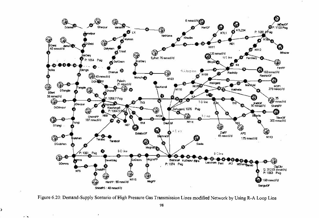
ctgClyQ: 312.01 mmsclld
. P: 1063 P,ig
160 """,clld-SonguGI'
MSher~.b
IIISl
J42
Nll1
o.C I!re
Lakshern Fenl
T.J ,in~
Nl03
Baktra# KuBepUr 88YaP:1074 P'ig
Sylhel: 76 mmscfld
MegPP
IKisOanj
Monohoe
8-0 !ine
~~LX - \i:l!!?
'ewnbag
HariPP:
SHddPS : 40 mmscfld
o
P,ig 0
Dh••.•.•• e40 mm,clld
DG~FF
laGanj
P: 1064 P'ig
'Elenge
N76
~ AerourISlpur
-0-.0"0-
Figure 6.20: Demand-Supply Scenario of High Pressure Gas Transmission Lines modified Network by Using R-A Loop Line
98:>
, "
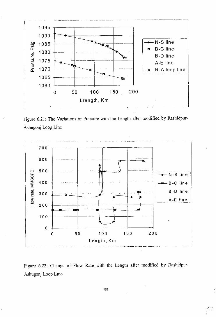
._- -- - -- --_._--~-_._. - ..... ~._---~-_._~.-----------------~-----
,.,,------- ------_.------ --u- _
10951090
.~ 10850... 1080~iil 1075en£ 107.0
10651060
o 50 100Lrength, Km
150 200
,----------- N-S line--B-C line
B-D lineA-E line
___ R-A loop line
Figure 6.21: The Variations of Pressure with the Length after modified by Rashidpur-
Ashugonj Loop Line
i
.. ------- .. .. . . .. .. . ----- .. .. -- -
(" ~
- .. - . .. .. .1 --_._- .. ---- ..
- .. . - -- ..
I . . .... ~. --~. - ....-..------1-- '-'-- --- ...- ----- _.__ ., ..
"'"-
--,. _. .- ..._- ---- ----_.-
~~.
700
600
0 500LL0en:2 400:2.,;- 300'"~;:.QLL 200
100
0a 50 100
Len 9 th, K m
150
__ N-S line
--.••- B -C lin e
B-D line
_'_.' A -_EJi_n~_.J
200
Figure 6.22: Change of Flow Rate with the Length after modified by Rashidpur-
Ashugonj Loop Line
99
/',

880.33 psig
BBeter: 991.09 rnsm3/d
HGF1: 7645.55 msm3fd
@,N117: 10:30.00 psig
ritBSdGF'
I
FenPP: 20.00 mmsctJd4530.70 msm3fd
ZiaFF: 45.00 mmscfJd
KaliGF:
KTL1: 707.92Jnsm3/d
Figure:6.23
~ 1'","
~.Ba'h,e' K,Bep", B;j,e Lok,hem Fen; J42 MSh"e; Bereb Fo,lderagC'y:
DJDTDSl: 76.00 mmscfJi
Nel:Kona:~
.~
BakhraGF:
'men
N115: 2.00 mmscf/d70.00 mmscfJd MegPP
Dhanua
,:':...E hj)~
ShiddP5: 40.00 mmscffd
;;:}~-J82 JB1
. ,OM,eFF
Elenga.Nolka line
Jamunaff: 4S.UO mmsc
Dlongi:
DJDevpur: 6.00
DJamal: 4.00 m~c
Ndka
BBari: 56.00 rr1rnscf/d
SanguGF: 4530.70 msm3Jd
Figure 6.23: Demand-Supply Scenario of Gas Transmission Lines modified by Using R-A Loop Line and mentioning Known Pressure atAshugonj
,.~ ,.~
100

,1,-,,-.. I-------~1'-~----'-~R__- ,-- - . ----
1150
1100
.Ql 1050(/)
0...1000
~iil 950(/)
~0... 900
850
800o 50 100
Length, Km
150 200
----- -_ ..__ ._----
__ N-S line
-D--B-ClineB-D lineA-E line
----*- R-A loop line
Figure 6.24: The Variations of Pressure with the Length after modified by Rashidpur-
Ashugonj Loop Line for Pressure Matching
6.7 Extension of Network up to Bheramara
The existing network will be expanded up to Bheramara in near future according to the
plan of Asian Development Bank. In Figure 6.25, 85 km 24" OD Nolka-Ishwardi-
Bheramara gas transmission pipeline is connected to the network to facilitate gas supply
to the planned industries in the Ishwardi EPZ and the power plants at Ishwardi and
Bheramara. Assuming the total loads in the Western region are 140 MMSCFD, the
network is simulated, The simulated results are tabulated in Appendix 8. Figure 6.26
shows the pressure drops along the major gas transmission lines. The inlet pressure at
North-South pipeline is 1090 psig. The pressure drops in the major transmission lines
are comparable to pressure drop which is obtained from the rule of thumb. Therefore,
there is no unusual pressure drop anywhere in the network after extension of network up
to Bheramara. Figure 6.27 shows the flow rate of major gas transmission lines. After
extension, the capacity of North-South line with Rashidpur-Ashugonj loop line will be
840 MMSCFD. The capacity of Ashugonj-Elenga line is 387 MMSCFD. Therefore,
there is no unreal situation in the network. The R-A loop line will increase the gas flow
between Rashidpur and Ashugonj points significantly.
101

HGF1
270 mmscl/d
agC~yQ: 258 mmscf/dP: 1062 Psig
N113APS175 mmscf/d
20mmscf/d
ShahjiPP
SanguGF
MShar~arab
~ B~ria
~-~
N61
J42
N4~ FenPP
Rashidp 160 mmscf/dRashidGF
S.C line
N111
Laksham Feni
Sylhel: 76 mmscf Id
MegPP : 77 mmsf/d
'ewnbag
Tarabo#
B-D line
N115HariPP: 80 mmsf/d
@
Tarabo
Elenga
N76
~Ae,pu,~~14 mmscf/d ~ LX
NetKona
DDemra
olka
DGulshan
DJDevpur
DTangileBBari46 mmscf/d
BheraPP40 mmscf/d
shurdi
,0~ShlddPS: 52 mmscf/d
Figure 6.25: Demand-Supply Scenario of High Pressure Gas Transmission Lines by extension of Network up to Bheramara
102

-- - ---------~-------- ----------- -----------------------
-+--N-S line--B-C line
B-D lineA-E line
__ R-A loop line
20015010050o
----- ---1----- ---._-,~- -_ .._._-- -------- -- -
10951090
.~ 1085c.. 1080~ 1075:J~ 1070£ 1065
10601055
Length, Km
Figure 6.26: Variation of Pressure Drop along Major Transmission Lines by Extension
of Network up to Bheramara
( -".- -_._--_.----~_._- --- - ----- -_. - -- - ----- j;--_. -------
_._- -- ------ -_.__ ._- ----- ---- --,,
- ._-- . - ---- -- -- _._- -- - -- _._- -- - --- ------------ - _.
I ~I
- ---- - - . ---- -- _._. - ---- - --- .-
"'"_ . .- . - ---- - ---_ .._-----
1-,
600
500
~~ 400u(/)
:::s:::s 300"'iii•...~ 2000G:
100
0o 50 100
Length,Km
150 200
-+-- N-S line
--B-C line
B-D line
A-E line
Figure 6.27: Change of Flow Rate along the Major Transmission Lines by Extension of
Network up to Bheramara
103
\...)

6.6 Extension of Network up to Khulna without Modification
In near future the demand of gas in the Western region will increase. According to the.
report of Asian Development Bank, the network should be extended up to Khulna
within 2010. Then the demand would reach 1900 MMSCFD (average). But GTCL
forecasted that the average gas demand would be 1700 MMSCFD to 1900 MMSCFD.
Therefore, this case has been studied using the demand as 1734 MMSCFD. In Figure
6.28, extending of transmission lines up to Khulna modifies the network. Assuming
total loads in the Western region are 320 MMSCFD, the scenario is simulated. The
major loads are assumed as follows:
Bheramara 70MMSCFD
Khulna 100MMSCFD
EPZ IOMMSCFD
Baghabaria 100MMSCFD
Shirajgonj 40MMSCFD
The simulated results are shown in Appendix 9.
The large pressure drop (I78 psig) in Ashugonj-Elenga line (Figure 6.29) is the
indication of inability of line to carry the expected flow. The pressure drop in Elenga-
Khulna line is 88 psig, which is also greater than the recommended pressure drop (20
psig). The pressure at Khulna is 749 psig. Therefore, it is not possible for Ashugonj-
Elenga line to carry the required flow.
The flow capacity in major transmission lines by extension of network withou! any
modification is shown in Figure 6.30. In Bakhrabad-bemra line, the flow rate is
increased at Dewanbag point because 41.85 MMSCFD flow is added at this point from
Demra and 53.17 MMSCFD flow is added at the same point from Sonargaon. The flow
situation of other transmission lines has been discussed previously.
Therefore, it is required to modify the network. The next cases are studied to overcome
the existing pressure problem.
104
./' ...

CgCity
F: 300 mmscf/dP: 982.9 Psig
aujdar
FenPP
A. JaBadGF
120 mmscl/d
K~
BBezar
: 250 mmscl/d
HasGF: 300 mmscf/d
ShahjiPP
SarabMSharai
KatjGF: 40 mmscl/d
J42
Manifold
8.C line
APS
Laksham Feni
N111
15 mmscf/d
N60
~r;GF
Khadim
Bakhrabadlt Ku8apur Bijra
MegPP
Sylhet: 80 mmscf/d
N115
oGaon
B-D line
,t•..E line
N76
J81
DDemra
~~ ••pur~~DJamal ~ MmenPP a LX NetKona
J ail'ur JJI
~Mymen40 mmscf/d
JamunaFFE,i., hp,::
Khulna
100 mmscf/d740.55 Psig
hurdi h'olka JB2
~
_ 160 mmscf/d
ShiddPS SanguGF
Figure 6.28: Demand-Supply Scenario of High Pressure Gas Transmission Lines by extension of Network up to Khulna without Modification
;;'(iii , F~
105

~:J(/)(/)
~0...
--'---
11001050
0> 1000'wc. 950
900850800750700
,-~.-
o 100 200Length, Km
300 400
-+- N-S line--B-C line
B-D lineA-E line
--R-A loop__ E-K line
Figure 6.29: The Variation Pressure of Major Transmission Lines by extension of
Network without any Modification
.- 1-- - - - ---- -- --
I!' ----------------_. ----- -- - - ------.
- ._--~_ .._- --- - -- - -- -- --- - - -- ---_.- -----
._ .._- -
- - --
- t--.: - ~ -- .------ -----,,-_.- ;:v-
~ ..~-._-- -- _.
'"_I
T
900800
0 700LL0 600(J):2: 500:2:Q) 400-ro•...::: 3000LL 200
1000
o 100 200 300
-+- B-C line1---- B-D line
A-E lineR-A loop I
__ E-K lineJ--N-S line--------------
Length, Km
Figure 6.30: Change of Flow Rate along the Major Transmission Lines by extension of
Network without any Modification
106
6.6.1 Extension of Network up to Khulna with Ashugonj-Dhanua Loop Line
According to the study of Asian Development Bank, it is clear that the existing network
will be extended up to Khulna within 2010. New power plant and fertilizer factory will
be set up in the Western region. Then demand of gas in this region will increase. Before
the extension to Khulna within the transmission lines, R-A loop line (69 km, 30" aD)
and Ashugonj-Dhanua loop line (69 km, 30" aD) will be completed on priority basis.
The network with Bheramara to Khulna transmission line is shown in Figure 6.3 J.
Assuming the total load in the Western region as 320 MMSCFD, the scenario is
simulated. The major loads are assumed as follows:
Bheramara 70MMSCFD
Khulna 100MMSCFD
EPZ 10MMSCFD
Baghabaria 100MMSCFD
Shirajgonj 40MMSCFD
The simulated results are tabulated in Appendix 10.
Figure 6.32 shows the pressure drops along the major gas transmission lines. The
pressure gradient in Ashgonj-Dhanua loop line is 0.0662 psig/km. The pressure gradient
in other lines is very close to the recommended pressure gradient. The pressure at
Khulna is 1039 psig. Therefore there is no shortage of pressure anywhere in the network
after completing Ashgonj-Dhanua loop line.
Figure 6.33 shows the simulated flow rates of major gas transmission lines. After
completing Ashgonj-Dhanua loop line, the capacity of North-South line with Rashidpur-
Ashugonj loop line will be 1116 MMSCFD. The capacity of Ashgonj-Dhanua line is
3689 MMSCFD. Then the capacity of Ashugonj-Elenga line with Ashgonj-Dhanua loop
line will be 559 MMSCFD.
Therefore, it is a possible option to construct the Ashgonj-Dhanua loop line for
increasing the gas flow in the Western Region in future.
107
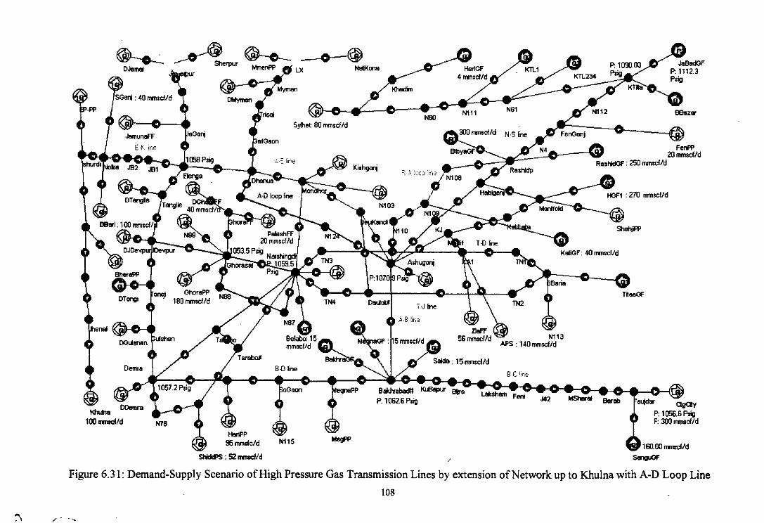
014<1'" ctgCllyP.1056.6 P1igF: 300 """ef/d
FenPl'20nmscf/d
250 rnrnocf/d
Tlos(lf
Ilor'"
SI10hjFP
_01
KatiGF: 40 mrmclld
Illart/old
.142
~Resl"lkt3F
B.C iin,:,
N61
N.5 rme
Lakstlem Feni
N1ll
15mmscl/d
N80
BokIv.bodlI ~r 8IjraP: 1062.6 p,ig
5yihot eo mmsefld
:oGaon
N1l5
B-Dline
N7B
~A._~~OJ.mol ~1Put MmenPl' ri LX NelKOIl8
~ - AMymenSGIlrj : 40 """ef/d
160.00 nmscf/d_:52nmscf/d ~
Figure 6.31: Demand-Supply Scenario of High Pressure Gas Transmission Lines by extension of Network up to Khulna with A-D Loop Line
108
:'\ ,

-+- N-S line-a-B-C line
B-D lineA-E line
__ R-A loop__ E-K line
--+- A-D loop
400300200Length,Km
100
--r ----~ -----~~l-
~
11001090
.gl 1080(/)
C-
Ol 1070,...::J 1060(/)(/)
Ol... 1050a.10401030
0
Figure 6.32: The Variation of Pressure along the Major Transmission Lines by
Extension of Network up to lUmina with Ashugonj-Dhanua Loop Line.
-+-N-S line-a-B-C line
B-D lineA-E line
__ R-A loop__ E-K line
--+- A-D line
300200
.1 _
100
-----:-- ..---d-" ------.._~.:---------
o
1000900800700600500400300200100
o
oLL()(/)~~Ol
~;;:oLL
Length, Km
Figure 6.33: Change of Flow Rate along the Major Transmission Lines by Extension of
Network up to Khulna with Ashugonj-Dhanua Line.
109
r\\"\.
6.6.2 Modification of Nolka to Khulna Line by Using Loop Line from Rashidpur-
Ashugonj Loop Line to Dhanua
To reduce the stress on the Ashugonj Station, the network has been modified with a loop
line from Rashidpur-Ashugonj loop line to Dhanua (69 KIn, 30" OD). Figure 6.34
shows the modification of Nolka to Khulna line by using loop line from Rashidpur-
Ashugonj loop line to Dhanua. Assuming the total load in the Western region is 320
MMSCFD, the scenario is simulated. The major loads are assumed as follows:
Bheramara 70 MMSCFD, Khulna 100 MMSCFD
EPZ 10 MMSCFD, Baghabaria 100 MMSCFD
Shirajgonj 40 MMSCFD
The simulated results are tabulated in Appendix 11.
Figure 6.35 shows the pressure drops along the major gas transmission lines. In North-
South line, the pressure gradient is 0.112 psig/km. The pressure gradient in Rashidpur- .
Ashugonj loop line, Bakhrabad-Demra line, Bakhrabad-Chittagong line, Ashugonj-
Elenga line and loop line from Rashidpur-Ashugonj loop line to Dhanua are 0.124
psig/km, 0.274 psig/km, 0.082 psig/km, 0.0934 psig/km and 0.062 psig/km respectively.
The pressure gradient in Bakhrabad-Demra line is larger due to the larger velocity of gas
in this line compare to others.
Figure 6.36 shows the flow capacity of major gas transmission lines. First jump of flow
in North-South line occurs at Rashidpur manifold station due to 250 MMSCFD gas is
added from Rashidpur gas field. Then it is divided into two parts; one part (741
MMSCFD) is passed through Rashidpur-Ashugonj loop line and other part (128
MMSCFD) is passed through N-S line. The loop line from Rashidpur-Ashugonj loop
line to Dhanua can carry 188 MMSCFD for which sharp decrease of flow is observed in
Rashidpur-Ashugonj loop line. Therefore, after completion of the proposed loop line,
the capacity of North-South line with Rashidpur-Ashugonj loop line will be 1117
MMSCFD.
Considering the above discussions, it is clear that it is possible to modify the network by
using loop line from Rashidpur-Ashugonj loop line to Dhanua.
110
~) ..
\"

HQfl270mrmcf/d
Tltl!llsGF300mmscf/d
SI,,".PI'36t1'll1'1SCfJd
'el4der QgCIy300 mrnsc:f/d
......,
KallGF : 40 mmtelld
N113
'*'ntfcld
•••••••••
200 """",f/d _ ----<li)KTL234 P:lIl9JP~ ;120='fd
KT~
BBelntr
Kl!tl"lata
J42
8.( 1'(;'"
F,
N111,0
- ----<!rIOF~ 4~.cfl
_dim
MegPP : 105 mrnscIJd
B.D line
,.SOGoon
R-A loop line toDhanu" loop line
ShId(FS : 52 nmscf/d
P:l059Psig <\-t:: Ilr,e
Bengo
".
~ ~SI1etP'" ~ --o---@DJIIIm!III .L..lelmeIlpur ~pp ./ LX NetKonll
40 rrmed/d Y ~ /"febi DMyme1'I•• Mymen
E ¥, 'jne D.De'IIJJUI'
1<h.AnlI: 100 RW'RIcl/d
folio
Sh ••70 mmtef/d
rJl'$$Of8
~
........,.,Figure 6.34: Demand-Supply Scenario of High Pressure Gas Transmission Lines modified by Using Loop Line from R-A Loop Line to Dhanua
/\III

--~-- ._.-_. __ .- ----- --- -----_. -- -----.- ----- -----_. -~-------------------
------_. __ ._------109510901085
.~ 1080Q. 1075[1! 1070::>~ 1065[1! 1060Q. 1055
10501045
o 50 100Length,Km
150 200
-+-N-S line___ B-C line
B-D lineA-E line
__ R-A loop line___ R-A to Dhanua
-------- ----_.- -------- -------- ------------------_._-_.--
Figure 6.35: The Pressure Drops of Major Transmission Lines of Nolka to Khulna
Pipeline Using Loop Line from Rashidpur-Ashugonj Loop Line to Dhanua
I 0u..o(f)
:2:2
1000800600400200
o
~.-I~----:
o 50 100Length, Km
150 200
__ N-S line
-- B-C line
B-D line
A-E line
---.*-R-A loop line
--------- -----_.--------------- ----------------- .----- _._._--
Figure 6.36: Change of Flow Rate along the Major Transmission Lines of Nolka to
Khulna Pipeline Using Loop Line from Rashidpur-Ashugonj Loop Line to Dhanua
112
----/"(
'.

6.8.3 Modification by Using Compressor Station at Monohordi
The construction of loop line is time consuming and lengthy process. Therefore, the
network can be modified alternatively. Using compressor station at Monohordi (1500
hp, 70% efficiency) instead of Ashugonj-Dhanua loop line the network can be modified
as shown in Figure 6.37. The simulated results are shown in Appendix 12.
The inlet pressure to the North.South pipeline is 1090 psig which is equal to the design
pressure. But the pressure drop in the North-South line is high. The pressure drops in the
other transmission lines are nearly equal to the recommended pressure drop. The
variation of pressure along the transmission lines is shown in Figure 6.38. Ashugonj-
Elenga line shows the effect of compressor at Monohordi.
113 I
\

Ferl'!'
_orJl """cf/d
••.••••. OgClyP:llm.1 P.igF: JlO rnmad/d
Sl\ehjPp: 36 mm.cf/d
TlasGFF: JlO mnm:f/d
MSMrai B«ab
KstlOF : 40 lTITl~f/d
J42
NIl1
8-C line
N.S line
Laklll1am Feli
N111N60
Bakh_ K1lIloIJU'BITe
D.J)TDSl: 90.00 mmscf/d
N76
~~_r~~0JemaI" ; 1=J'>..."'-LX NetKona
HerI'P
: 95 mmsl/d W F: 160 nmad/dSltiP.; : 52 rnmad/d SanguClF
Figure 6.37: Demand-supply Scenario of High Pressure Gas Transmission Lines modified Final Network by Using Compressor Station aMonohordi
.~.114

11001080
OJ"iii 1060c.~ 1040~ 1020VJ~ 1000D..
980960
o 100 200
Length, Km
300 400
-+-N-S line__ B-C line
B-D lineA-E line
--*- R-A loop--E-K line
---------- - _._"---~-----------_._----_._----- --
Figure 6.38: The Variation of Pressure along the Major Transmission Lines modified by
Using Compressor Station at Monohordi
115

Chapter 7
DISCUSSIONS
There are twenty-two gas fields in Bangladesh. At present, gas is lifted from twelve gas
fields. The peak lifted gas in June 2000 was 1013 MMSCFD. After lifting natural gas
from the fields, the gas Companies produce pipeline quality gas through process plants.
Then, the treated gases are delivered to the transmission pipeline through fiscal meter.
The Orifice meter is used as a fiscal meter and for monitoring accurately the flow
recorder is connected with the orifice meter. Beyond this, the hourly calculations of
flowing gas are recorded from the gas fields to the transmission line.
To improve the supply/demand balance and to enhance the satisfaction of gas
customers, Petrobangla has moved progressively from four separate systems (JFA, TFA,
BFA and WFA) to an integrated transmission network. The reliability and security of
gas supply in the national gas grid is largely dependent on the following pipelines:
1. 174 km, 24" OD North-South Gas Transmission Pipeline
2. 12" OD 38 km Ashuganj- Habiganj Gas Transmission Pipeline
3. 14" OD 58 km Titas-Narshindi-Demra Gas Transmission Pipeline
4. 16"/14" OD 82.81 km Titas-Narshindi-Joydevpur Gas Transmission Pipeline
5. 20" OD 48 km Bakhrabad-Demra Gas Transmission Pipeline
6. 20" OD 48 km offshore Sub Sea Sangu Gas Transmission Pipeline
7. 14" OD 15 km Jalalabad - Kailashtilla Gas Pipeline
8. 20" OD 18 km Beanibazar-Kailashtilla Pipeline
9. II" OD 37 km Salda- Bakhrabad Pipeline
10. 8" OD 28 km Meghna Gas Field- Bakhrabad Pipeline
If the transmission network is carefully analyzed it appears that Ashuganj is the focal
points of the National Gas Grid. Two key locations of Ashuganj are mainline Valve
Station-3 of Titas-Narshindi-Demra transmission pipeline and Manifold station of
GTCL. Gas from the Northern Gas Fields (Beanibazar, Jalalabad, Kailashtilla,
.Rashidpur, Habiganj) are being transported through the North-South pipeline to
Ashuganj Manifold Station of GTCL from where it is further transmitted to Titas
116

franchise area (TFA) and Bakhrabad franchise area (BFA) through Brahmaputra Basin
pipe line and Ashuganj- Bakhrabad transmission pipe lines respectively. From
Bakhrabad Gas Field, Bakhrabad-Chittagong Pipeline transports part of the required gas
for Chittagong. The remaining gases for Chittagong is supplied from Salda, Meghna and
Sangu gas fields. The mother trunk line i.e. North- South Pipeline has a design capacity
of 330 MMSCFD. However considering the staggered nature of input into the pipeline
and adjusting the terminal pressures at various in-take points and at Ashuganj it may be
possible to transport 400 MMSCFD through the pipeline. Currently it is transporting
approximately 353-380 MMSCFD, which merely cater to the downstream gas demand.
During the past few years Bakhrabad gas field has been experiencing rapid pressure
decline and increased water cuts in the wells. As a result, some wells have been shut off
and some have been re-completed. In the year 1992 this field produced in its peak at an
average 195 MMSCFD. In 1998, only five wells were producing from three sands at the
rate of 50 MMSCFD. At present, the field is delivering gas at the rate of 35 MMSCFD
at 600 psig. Currently Bakhrabad gas field is connected to the network system by
reducing the pressure of Bakhrabad to Demra pipeline. If the line pressure is not reduced
the Bakhrabad gas field could not be connected to the transmission system without
compressor. When the proposed power plant will be started in peak production, the
pressure of B-D line needs to be increased. Then Bakhrabad gas field will face a lot of
pressure problem. If BGF is stopped production, it will not be possible to reach
recoverable reserve and it will be a dead well. To overcome this problem, a compressor
station should be set up at Bakhrabad gas field. The power of compressor must be
greater than 700 hp at 70 % efficiency.
The demand of gas was increasing day by day in fertilizer, power, industry and
commercial sectors. If the proposed power plants start their production, the demand of
gas will increase. To recover this demand, it is necessary to lift gas at higher rate.
Therefore, 856 MMSCFD will be delivered from JFA. The maximum allowable
operating pressure of the North- South p-ipeline is 1135 psig, its maximum inlet pressure
1090 psig and the normal pressure in A-shugonj is 850 psig. From Appendix 3, it is clear
that N-S pipeline and Gas Fields experience unexpected pressure that is greater than its
design pressure to reach the desired flow rate. From the simulated result, it is clear that
after completing R-A loop line, the capacity of N-S pipeline with R-A loop line will be
117
increased and become 850 MMSCFD. Therefore, it is necessary to construct a loop line
from Rashidpur to Ashugonj to deliver excess flow at design pressure on priority basis.
If a new loop line from R-A loop line to Dhanua is constructed, the capacity ofN-S line
with R-A loop line will be 790 MMSCFD. Even though the pressure drop in the major
transmission lines will be low to meet the demand of Western Region. Therefore, R-A
loop line to Dhanua loop line needs to be completed after completing R-A loop line.
Now Ashugonj is the main points of the National Gas Grid. To reduction stress on
Ashugonj station, it is required to construct loop line from R-A loop line to Dhanua loop
line. There will be no problem in gas transmission system when the network will be
extended up to Bheramara.
Within 20 I 0, the existing network will be expanded up to Khulna according to the
report of Asian Development Bank. Then the gas demand would reach 1900 MMSCFD
(average). Then the capacity of A-E line will have to be increased. If no loop line is
constructed with A-E line, unexpected pressure drop will occur in A-E line (187 psig).
Therefore, it is required to modify the network. To overcome the constraints of A-E line,
three cases have been studied: i) A-D loop line ii) loop line from R-A loop line to
Dhanua and iii) compressorstation at Monohordi. If A-D loop line is constructed, there
is no shortage of pressure in the network. Therefore, it is possible to modify the network
with A-D loop line. If a loop line from R-A loop line to Dhanua is constructed, large
pressure gradient is observed in B-D line due to the larger velocity of gas in this line. To
minimize pressure problem in Western region a compressor station may be set up at
Monohordi. Therefore, according to the over all study, it will be better to construct A-D
loop line or loop line from R-A loop line to Dhanua for reducing the stress on Ashugonj
metering station.
118
(

Chapter 8
CONCLUSIONS AND RECOMMENDATIONS
8.1 Conclusions
After analyzing the integrated gas transmission network of Bangladesh, the following
conclusion can be drawn:
I. Simulated results compare well with the actual data. Therefore, the network can be
used to predict the future demand/supply scenario under existing and future supply
and loads.2. The results show that effective pipeline diameter of major transmission lines have
decreased due to condensate accumulation. Hence pigging is necessary.
3. The maximum capacity of N-S pipeline is 400 MMMSCFD. Significant flow
constraints and pressure drop arise in this line when the demand of gas is increased.
4. Rashidpur-Ashugonj loop line is essential to supply the growing gas demand. It will
increase the capacity of the North-South pipeline by 456 MMSCFD.
5. Analysis shows that it is a better option to install a compressor station at Bakhrabad
to transmit the low-pressure gas of the field through the high-pressure pipeline.
6. After completing R-A loop line, another loop line from R-A loop line to Dhanua or
A-D loop line is required to minimize pressure problems in the transmission lines.
7. To extent of network up to Khulna, R-A loop line and loop line from R-A loop lines
to Dhanua or A-D loop line must be completed on priority basis.
8. To minimize pressure problem in Western region a compressor station may be set up
at Monohordi after completing R-A loop line instead of A-D loop line or loop line
from R-A loop line to Dhanua.
9. To meet the future gas demand of the Western region, the results show that another
loop line is necessary from Rashidpur-Ashugonj loop line to Dhanua. It will increase
the supply of Ashugonj-Elenga pipeline by 175 MMSCFD.
119
8.2 Recommendations
1. To remove the constraint ofN-S pipeline, a loop line from Rashidpur to Ashugonj is
to be constructed in priority basis.
2. The author strongly recommended for setting up a compressor station at Bakhrabad
gas field.
3. For creating stability of gas supply in the Western region, a loop line is being set up
from R-A loop line to Dhanua.
120 () . {«
I\. ,
-}
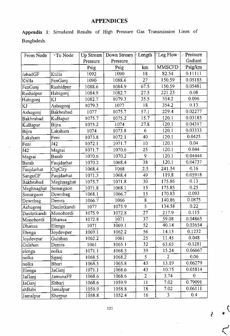
APPENDICES
Appendix 1: Simulated Results of High Pressure Gas Transmission Lines of
Bangladesh.
From Node "To Node Up Stream Down Stream . . Lengtn 'Leg Flow ,PressurePressure Pressure . . (}adiant
Psig Psig km MMSCFD PsiglkmJabadGF Ktilla 1092 1090 18 82.54 0.11111Ktilla FenGanj 1090 1088.6 27 150.59 0.05185FenGanj Rashidpur 1088.6 1084.9 67.5 150.59 0.05481Rashidpur Habigonj 1084.9 1082.7 27.5 221.23 0.08Habigonj KJ 1082.7 1079.3 35.5 354.2 0.096KJ Ashugonj 1079.3 1077 18 354.2 0.13Ashugonj Bakhrabad 1077 1075.7 57.1 229.4 0.02277Bakhrabad KuBapur 1075.7 1075.2 15.7 120.1 0.03185KuBapur Bijra 1075.2 1074 27.8 120.1 0.04317
Bijra Laksham 1074 1073.8 6 120.1 0.03333Laksham Feni 1073.8 1072.1 40 120.1 0.0425
Feni J42 1072.1 1071.7 10 120.1 0.04J42 Msgrai 1071.7 1070.6 25 120.1 0.044Msgrai Barab 1070.6 1070.2 9 120.1 0.04444Barab Faujdarhat 1070.2 1068.4 38 120.1 0.04737Faujdarhat CtgCity 1068.4 1068 2.5 241.34 0.16SanguGF Faujdarhat 1071.3 1068.4 49 119.8 0.05918Bakhrabad Meghnaghat 1075.7 1071.8 30 175.86 0.13Meghnaghat Sonar£!aon 1071.8 1068.1 15 175.85 0.25Sonargaon Dewnbag 1068.1 1066.7 15 170.83 0.093Dewnbag Demra 1066.7 1066 8 140.86 0.0875Ashugonj Daulotkandi 1077 1075.9 5 134.58 0.22Daulotkandi Monohordi 1075.9 1072.8 27 217.9 0.115Monohordi Dhanua 1072.8 1071 37 59.08 0.04865Dhanua Elenga 1071 1069.1 52 40.14 0.03654
Elenga Joydevpur 1069.1 1062.2 56 14.13 0.1232Joydevpur Gulshan 1062.2 1061 25 11.45 0.048Gulshan Demra 1061 1065.1 32 63.65 -0.1281elenga nolka 1071.1 1068.5 39 15.24 0.06667nolka Sganj 1068.5 1068.2 5 2 0.06nolka Bbari 1068.5 1065.8 43 13.19 0.06279
Elenga JaGanj 1071.1 1068.6 43 10.75 0.05814JaGanj JamunaFF 1068.6 1068.6 2 3.74 0JaGanj Shbari 1068.6 1059.9 11 7.02 0.79091shBabi Jamalpur 1059.9 1058.8 18 7.02 0.06111Jamalpur Sherpur 1058.8 1052.4 16 3 0.4
121
I

Dhanua GafGaon 1072 1071.7 19 18.94 0.01579GafGaon Trishal 1071.7 1070.4 20.004 18.94 0.06499Trisa1 mymen 1070.4 1065.5 16 18.94 0.30625Mymen LX 1065.5 1060.6 8 16.94 0.6125LX Mymenpp 1060.6 1058.2 5 14.88 0.48Lx Neykona 1060.6 1053.8 32.5 2 0.20923Monohordi kisGanj 1073.8 1071.5 36 2 0.06389KA1 APS 1076.1 1015.1 1.5 100.99 40.6667KA1 ZiaFF 1076.1 1075.9 2.4 0.005 0.08333Dewnbag hariPP 1066.7 1066.7 1.58 29.86 0FenGanj fenpp 1088.6 1088.6 0.5 0.005 0RashidGF Rashidpur 1085.3 1084.9 1.9 70.62 0.21053HGF1 Manifold 1085.3 1085.3 0.006 187.9 0Manifold ShahjiPP 1085.3 952.2 2.5 36.61 53.24Manifold Habigonj 1085.3 1082.7 1 132.24 2.6Manifold Katihata 1085.3 1078.5 42 17.47 0.1619Katihata Manif 1078.5 1076.1 11.5 17.47 0.2087Manif Ashuganj 1076.1 1077 2 35.97 -0.45N61 Ktilla 1090.01 1090 0.02 67.97 0.5N111 N61 1088.9 1090.01 28 0.116 -0.0396Nl11 N105 1088.9 1088.7 2.082 12.82 0.09606N105 Sylhet 1088.7 1088.68 0.03 17.28 0.66667HariGF N105 1089.2 1088.7 12 3.47 0.04167SaldaGf Bakhrabad 1088.3 1075.7 35 15.12 0.36MeghnaGF Bakhrabad 1117.7 1075.7 28 17.14 1.5TitasGf Bbaria 1160.6 1092.4 1 303.2 68.2Bbaria . TN1 1092.4 1090.8 1 152.4 1.6Bbaria TN2 1092.4 1091.4 1 75.45 1TN1 KA1 1090.8 1076.1 14.1 152.4 1.04255KAI TN3 1076.1 1073.6 7 32.9 0.35714TN3 Nars 1073.6 1066.8 30 32.9 0.22667TN2 Daulot# 1091.4 1076 16 145.8 0.9625Daulot# TN4 1076 1068 29 62.49 0.27586TN4 Nars' 1068 1067.8 1 62.49 0.2Nars Tarabo 1067.8 1066.5 20 2.87 0.065Tarabo Demra 1066.5 1065.1 12 4.33 0.11667Nars Tarabo# 1066.8 1066.1 40 21.91 0.0175Tarabo# ShiddPP 1066.1 1066 5 20.45 0.02ShiddPP ShiddPS 1066 1066 0.0003 14.62 0ShiddPP N76 1066 1065.7 10 5.81 0.03N76 Demra 1065.7 1065.1 10 5.81 0.06Nras Ghorasal 1066.8 1060.1 8.4 233.7 0.79762Ghorasal GhoraPP 1060.1 760.38 0.4 175.54 749.3Ghorasal GhoraFF 1060.1 1051.8 8.4 55.31 0.9881GhoraFF DGhoraFF 1051.8 1051.8 0.0003 43.2 0GhoraFF PalashFF 1051.8 1051 0.8 12 1
122

Monohordi Nars 1073.8 1066.8 32 151.8 0.21875Daulot# Daulotkandi 1076 1075.9 0.1 83.11 1BelaboGF Nars 1084.9 1067.8 13 16.31 1.31538
Appendix 2: Simulated Results of High Pressure Gas Transmission Lines of
Bangladesh modified by Known Pressure at Ashugonj.
From Node To Node Up Stream Down Stream . .'Len~ 'Leg Flow ,Pressure".' "
Pressure Pressure 0
. Gadianto. 0
'Psig 'Psig " km MMSCFD PsigfkmJabadGF Ktilla 1108.6 1090 18 82.66 1.03333Ktilla FenGanj 1090 1075.1 27 57.17 0.55185FenGanj Rashidpur 1075.1 1035 67.5 57.16 0.59407Rashidpur Habigonj 1035 1005 27.5 127.8 1.09091Habigonj KJ 1005 948.44 35.5 242.98 1.59324KJ Ashugonj 948.44 915.79 18 242.98 1.81389Ashugonj Bakhrabad 915.79 891.17 57.1 188.88 0.43117Bakhrabad KuBapur 891.17 876.67 15.7 122.98 0.92357KuBapur Bijra 876.67 836.53 27.8 122.98 1.44388Bijra Laksham 836.53 830.14 6 122.98 1.065Laksham Feni 830.14 794.82 40 122.98 0.883Feni J42 794.82 781.35 10 122.98 1.347J42 Msgrai 781.35 756.07 25 122.98 1.0112Msgrai Barab 756.07 743.5 9 122.98 1.39667Barab Faujdarhat 743.5 701.42 38 122.98 1.10737Faujdarhat CtgCity 701.42 700 2.5 242.79 0.568SanguGF Faujdarhat 710.35 701.42 49 119.8 0.18224Bakhrabad Meghnaghat 891.17 834.73 30 132.41 1.88133Meghnaghat Sonargaon 834.73 790.54 15 132.41 2.946Sonargaon Dewnbag 790.54 761.72 15 127.4 1.92Dewnbag Demra 761.72 750.01 8 97.57 1.46375Ashugonj Daulotkandi 915.79 912.36 5 151.02 0.686Daulotkandi Monohordi 912.36 895 27 184.83 0.643Monohordi Dhanua 895 880.0J 37 87.97 0.41Dhanua Elenga 880.01 864.98 52 69.16 0.29Elenga Joydevpur 864.98 793.74 56 4.03 1.27214Joydevpur Gu1shan 793.74 730.48 25 32.34 2.5304Gulshan Demra 730.48 750.01 32 19.42 -0.6103elenga no1ka 864.98 862.53 39 15.13 0.06282nolka Sganj 862.53 862.12 5 2 0.082nolka Bbari 862.53 859.68 43 13.19 0.06628Elenga JaGanj 864.98 861.85 43 10.7 0.07279JaGanj JamunaFF 861.85 861.85 2 3.74 0JaGanj Shbari 861.85 859.22 11 6.97 0.23909
123
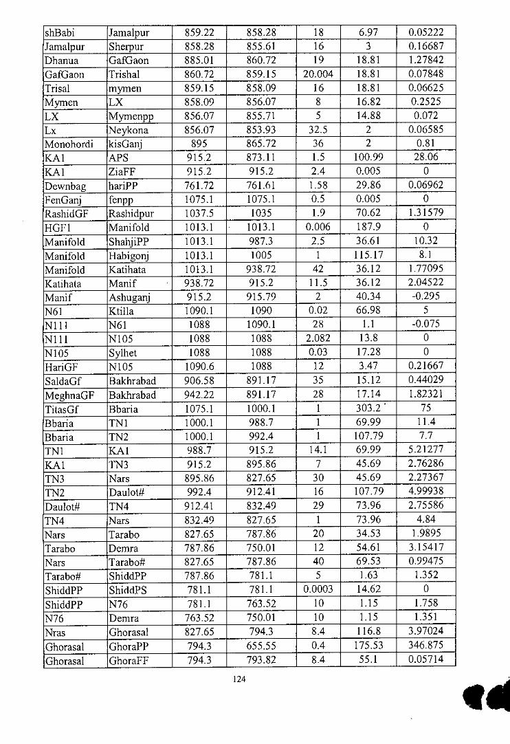
shBabi Jamalpur 859.22 858.28 18 6.97 0.05222Jamalpur Sherpur 858.28 855.61 16 3 0.16687Dhanua GafGaon 885.01 860.72 19 18.81 1.27842GafGaon Trishal 860.72 859.15 20.004 18.81 0.07848Trisal mymen 859.15 858.09 16 18.81 0.06625Mymen LX 858.09 856.07 8 16.82 0.2525LX Mymenpp 856.07 855.71 5 14.88 0.072Lx Neykona 856.07 853.93 32.5 2 0.06585Monohordi kisGanj 895 865.72 36 2 0.81KAI APS 915.2 873.11 1.5 100.99 28.06KAI ZiaFF 915.2 915.2 2.4 0.005 0Dewnbag hariPP 761.72 761.61 1.58 29.86 0.06962FenGanj fenpp 1075.1 1075.1 0.5 0.005 0RashidGF Rashidpur 1037.5 1035 1.9 70.62 1.31579HGFI Manifold 1013.1 1013.1 0.006 187.9 0Manifold ShahjiPP 1013.1 987.3 2.5 36.61 10.32Manifold Habigonj 1013.1 1005 1 115.17 8.1Manifold Katihata 1013.1 938.72 42 36.12 1.77095Katihata Manif 938.72 915.2 11.5 36.12 2.04522Manif Ashuganj 915.2 915.79 2 40.34 -0.295N61 Ktilla 1090.1 1090 0.02 66.98 5N111 N61 1088 1090.1 28 1.1 -0.075Nll1 Nl05 1088 1088 2.082 13.8 0NI05 Sylhet 1088 1088 0.03 17.28 0HariGF NI05 1090.6 1088 12 3.47 0.21667SaldaGf Bakhrabad 906.58 891.17 35 15.12 0.44029MeghnaGF Bakhrabad 942.22 891.17 28 17.14 1.82321TitasGf Bbaria 1075.1 1000.1 1 303.2 . 75Bbaria TNI 1000.1 988.7 1 69.99 11.4Bbaria TN2 1000.1 992.4 1 107.79 7.7TNI KAI 988.7 915.2 14.1 69.99 5.21277KAI TN3 915.2 895.86 7 45.69 2.76286TN3 Nars 895.86 827.65 30 45.69 2.27367TN2 Daulot# 992.4 912.41 16 107.79 4.99938Daulot# TN4 912.41 832.49 29 73.96 2.75586TN4 Nars 832.49 827.65 1 73.96 4.84Nars Tarabo 827.65 787.86 20 34.53 1.9895Tarabo Demra 787.86 750.01 12 54.61 3.15417Nars Tarabo# 827.65 787.86 40 69.53 0.99475Tarabo# ShiddPP 787.86 781.1 5 1.63 1.352ShiddPP ShiddPS 781.1 781.1 0.0003 14.62 0ShiddPP N76 781.1 763.52 10 1.15 1.758N76 Demra 763.52 750.01 10 1.15 1.351Nras Ghorasal 827.65 794.3 8.4 116.8 3.97024Ghorasal GhoraPP 794.3 655.55 0.4 175.53 346.875Ghorasal GhoraFF 794.3 793.82 8.4 55.1 0.05714
124

GhoraFF DGhoraFF 793.82 793.81 0.0003 43.2 33.3333
GhoraFF PalashFF 793.82 793.17 0.8 12 0.8125
Monohordi Nars 901.13 827.65 32 89.9 2.29625
Daulot# Daulotkandi 912.41 912.36 0.1 33.83 0.5
BelaboGF Nars 851.24 827.65 13 16.31 1.81462
Appendix 3: Simulated Results of High Pressure Transmission Lines Using Known
Pressure at Bakhrabad Gas Field.
From Node To Node Up Stream Down Stream Length Leg Flow Pressure
Pressure, Pressure, Psig km MMSCFD GadiantPsig Psildkm
JabadGF Ktilla 1098.5 1090 18 83.52 0.47222
Ktilla FenGanj 1090 1085.6 27 150.58 0.16296
FenGanj Rashidpur 1085.6 1055.7 67.5 150.58 0.44296
Rashidpur Habigonj 1055.7 1035.3 27.5 221.23 0.74182
Habigonj KJ 1035.3 980.3 35.5 361.14 1.5493
KJ Ashugonj 1035.3 917.45 18 361.14 6.54722
Ashugonj Bakhrabad 917.45 907.66 57.1 91.01 0.17145
Bakhrabad KuBapur 907.66 902.77 15.7 121.5 0.31146
KuBapur Bijra 902.77 894.03 27.8 121.5 0.31439
Bijra Laksham 894.03 892.51 6 121.5 0.25333
Laksham Feni 892.51 875.74 40 121.5 0.41925
Feni J42 875.74 868.78 10 121.5 0.696
J42 Msgrai 868.78 851.4 25 121.5 0.6952
Msgrai Barab 851.4 843.16 9 121.5 0.91556
Barab Faujdarhat 843.16 808.4 38 121.5 0.91474
Faujdarhat CtgCity 808.4 795.2 2.5 241.33 5.28
SanguGF Faujdarhat 860.15 808.4 49 119.8 1.05612
Bakhrabad Meghnaghat 907.66 622.2 30 34.87 9.51533
Meghnaghat Sonargaon 622.2 620.43 15 34.86 0.118
Sonargaon Dewnbag 620.43 618.77 15 29.86 0.11067
Dewnbag Demra 618.77 618.77 8 0 0
Ashugonj Daulotkandi 917.45 910.83 5 255.52 1.324
Daulotkandi Monohordi 910.83 895.2 27 262.93 0.57889
Monohordi Dhanua 895.2 875.97 37 97.38 0.51973
Dhanua E1enga 875.97 850.48 52 78.48 0.49019
Elenga Joydevpur 850.48 776.24 56 40.5 1.32571
Joydevpur Gulshan 776.24 763.24 25 0.348 0.52
Gulshan Demra 763.24 765.3 32 51.52 -0.0644
elenga nolka 870.48 860.3 39 15.21 0.26103
nolka Sganj 860.3 860 5 2 0.06
nolka Bbari 860.3 855.85 43 13.19 0.10349
Elenga JaGanj 850.48 865.4 43 10.75 -0.347
125

JaGanj JamunaFF 865.4 865.3 2 3.74 0.05JaGanj Shbari 865.4 863.81 11 7.01 0.14455shBabi Jamalpur 863.81 857.69 18 7.01 0.34Jamalpur Sherpur 857.69 853.29 16 3 0.275Dhanua GafGaon 875.97 865.25 19 18.9 0.56421GafGaon Trisha1 865.25 859.58 20.004 18.9 0.28344Trisal mymen 859.58 855.04 16 18.9 0.28375Mymen LX 855.04 840.96 8 16.9 1.76
LX Mymenpp 840.96 840.06 5 14.88 0.18
Lx Neykona 840.96 837.17 32.5 2 0.11662
Monohordi kisGanj 895.2 868.62 36 2 0.73833
KA1 APS 870.44 504.82 1.5 100.99 243.747
KA1 ZiaFF 870.44 870.44 2.4 0 0Dewnbag hariPP 618.77 617.95 1.58 29.86 0.51899FenGanj fenpp 1085.6 617.95 0.5 0 935.3
RashidGF Rashidpur 1089.1 1055.7 1.9 70.62 17.5789
HGF1 Manifold 1073.3 1073.2 0.006 187.9 16.6667Manifold ShahjiPP 1073.2 1047.8 2.5 36.61 10.16
Manifold Habigonj 1073.2 1035.3 1 139.89 37.9
Manifold Katihata 1073.2 1012.7 42 11.39 1.44048
Katihata Manif 1012.7 980.3 11.5 11.39 2.81739
Manif Ashuganj 980.3 917.45 2 11.39 31.425
N6l Ktilla 1091 1090 0.02 66.98 50N111 N61 1088.9 1091 28 1.1 -0.075NIl! N105 1088.1 1085.9 2.082 13.8 1.05668
N105 Sylhet 1085.9 1085.4 0.03 17.28 16.6667
HariGF N105 1089.4 1085.9 12 3.47 0.29167
SaldaGf Bakhrabad 922.78 907.66 35 15.12 0.432MeghnaGF Bakhrabad 957.78 907.66 28 17.14 1.79
TitasGf Bbaria 1087.5 1005 1 303.2 82.5Bbaria TN1 1005 996.4 1 173.32 8.6Bbaria TN2 1005 999.9 1 124.88 5.1TN1 KA1 996.4 870.44 14.1 173.32 8.93333KA1 TN3 870.44 860.33 7 72.32 1.44429TN3 Nars 860.33 820.31 30 72.32 1.334
TN2 Daulot# 999.9 910.86 16 124.88 5.565Daulot# TN4 910.86 820.31 29 117.48 3.12241TN4 Nars 820.31 817.29 1 117.48 3.02Nars Tarabo 817.29 803.09 20 47.76 0.71Tarabo Demra 803.09 765.3 12 4.32 3.14917Nars Tarabo# 817.29 803.09 40 105.32 0.355
Tarabo# ShiddPP 803.09 802.7 5 148.76 0.078ShiddPP ShiddPS 802.7 802.69 0.0003 14.62 33.3333ShiddPP N76 802.7 801.1 10 134.15 0.16N76 Demra 801.1 765.3 10 134.15 3.58Nras Ghorasal 817.29 771.99 8.4 206.58 5.39286
126
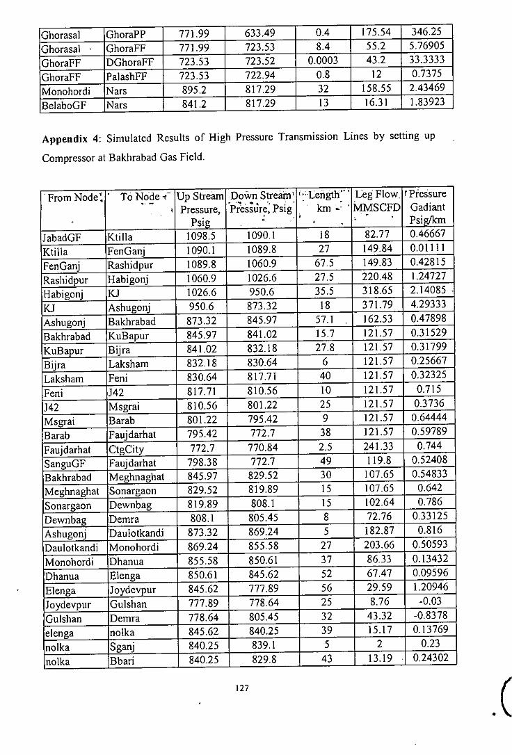
Ghorasa1 GhoraPP 771.99 633.49 0.4 175.54 346.25
Ghorasal GhoraFF 771.99 723.53 8.4 55.2 5.76905
GhoraFF DGhoraFF 723.53 723.52 0.0003 43.2 33.3333
GhoraFF PalashFF 723.53 722.94 0.8 12 0.7375
Monohordi Nars 895.2 817.29 32 158.55 2.43469
BelaboGF Nars 841.2 817.29 13 16.31 1.83923
Appendix 4: Simulated Results of High Pressure Transmission Lines by setting up
Compressor at Bakhrabad Gas Field.
From Node: . To Node~- Up Stream Down Stream' ':Leilgth:- . Leg Flow. rPressure. '.......", ',;, Pressure, Pressur~, Psig . km." MMSCFD Gadiant,Psillikm. Psig . . . ,-
JabadGF Ktilla 1098.5 1090.1 18 82.77 0.46667
Ktilla FenGanj 1090.1 1089.8 27 149.84 0.01111
FenGanj Rashidpur 1089.8 1060.9 67.5 149.83 0.42815
Rashidpur Habigonj 1060.9 1026.6 27.5 220.48 1.24727
Habigonj KJ 1026.6 950.6 35.5 318.65 2.14085 .
KJ Ashugonj 950.6 873.32 18 371.79 4.29333
Ashugonj Bakhrabad 873.32 845.97 57.1 162.53 0.47898
Bakhrabad KuBapur 845.97 841.02 15.7 121.57 0.31529
KuBapur Bijra 841.02 832.18 27.8 121.57 0.31799
Bijra Laksham 832.18 830.64 6 121.57 0.25667
Laksham Feni 830.64 817.71 40 121.57 0.32325
Feni J42 817.71 810.56 10 121.57 0.715
J42 Msgrai 810.56 801.22 25 121.57 0.3736
Msgrai Barab 801.22 795.42 9 121.57 0.64444
Barab Faujdarhat 795.42 772.7 38 121.57 0.59789
Faujdarhat CtgCity 772.7 770.84 2.5 241.33 0.744
SanguGF Faujdarhat 798.38 772.7 49 119.8 0.52408
Bakhrabad Meghnaghat 845.97 829.52 30 107.65 0.54833
Meghnaghat Sonargaon 829.52 819.89 15 107.65 0.642
Sonargaon Dewnbag 819.89 808.1 15 102.64 0.786
Dewnbag Demra 808.1 805.45 8 72.76 0.33125
Ashugonj Daulotkandi 873.32 869.24 5 182.87 0.816
Daulotkandi Monohordi 869.24 855.58 27 203.66 0.50593
Monohordi Dhanua 855.58 850.61 37 86.33 0.13432
Dhanua Elenga 850.61 845.62 52 67.47 0.09596
Elenga Joydevpur 845.62 777.89 56 29.59 1.20946
Joydevpur Gulshan 777.89 778.64 25 8.76 -0.03
Gulshan Demra 778.64 805.45 32 43.32 -0.8378
elenga nolka 845.62 840.25 39 15.17 0.13769
nolka Sganj 840.25 839.1 5 2 0.23
nolka Bbari 840.25 829.8 43 13.19 0.24302
127 .(

Elenga JaGanj 845.62 842.73 43 10.73 0.06721
JaGanj JamunaFF 842.73 842.7 2 3.74 0.015
JaGanj Shbari 842.73 842.05 11 6.99 0.06182
shBabi Jamalpur 842.05 836.95 18 6.99 0.28333
Jamalpur Sherpur 836.95 832.32 16 3 0.28938
Dhanua GafGaon 850.61 844.07 19 18.86 0.34421
GafGaon Trishal 844.07 837.07 20.004 18.86 0.34993
Trisal mymen 837.07 831.44 16 18.86 0.35188
Mymen LX 831.44 817.44 8 16.86 1.75
LX Mymenpp 817.44 817.41 5 14.88 0.006
Lx Neykona 817.44 813.11 32.5 2 0.13323
Monohordi kisGanj 855.58 841.04 36 2 0.40389
KAI APS 836.96 400 1.5 100.99 291.307
KAI ZiaFF 836.96 836.96 2.4 0 0
Dewnbag hariPP 808.1 808.1 1.58 0 0
FenGanj fenpp 1089.8 1089.8 0.5 0 0
RashidGF Rashidpur 1089.3 1060.9 1.9 70.62 14.9474
HGFI Manifold 1073.1 1073 . 0.006 187.9 16.6667
Manifold ShahjiPP 1073 1047.5 2.5 36.61 10.2
Manifold Habigonj 1073 1026.6 1 98.16 46.4
Manifold Katihata 1073 1016.6 42 53.13 1.34286
Katihata Manif 1016.6 915.8 11.5 53.13 8.76522
Manif Ashuganj 915.8 873.32 2 53.13 21.24
N61 Ktilla 1090.2 1090.1 0.02 66.98 5
Nlll N61 1090.1 1090.2 28 1.1 -0.0036
Nlll NI05 1090.1 1090 2.082 13.8 0.04803
NI05 Sy1het 1090 1089 0.03 17.28 33.3333
HariGF NI05 1090.6 1090 12 3.47 0.05
SaldaGf Bakhrabad 846.24 845.97 35 15.12 0.00771
MeghnaGF Bakhrabad 899.73 845.97 28 17.14 1.92
TitasGf Bbaria 1000.9 961.28 1 303.2 39.62
Bbaria TNI 961.28 944 1 145.6 17.28
Bbaria TN2 961.28 946.61 1 152.6 14.67
TNI KAI 944 836.96 14.1 145.6 7.59149
KAI TN3 836.96 832.6 7 44.6 0.62286
TN3 Nars 832.6 813.67 30 44.6 0.631
TN2 Daulot# 946.61 869.33 16 152.6 4.83
Daulot# TN4 869.33 816.09 29 131.81 1.83586
TN4 Nars 816.09 813.67 1 131.81 2.42
Nars Tarabo 813.67 810.17 20 24.52 0.175
Tarabo Demra 810.17 805.45 12 29.44 0.39333
Nars Tarabo# 813.67 810.17 40 47.7 0.0875
Tarabo# ShiddPP 810.17 809.75 5 42.78 0.084
ShiddPP ShiddPS 809.75 809.1 0.0003 14.62 2166.67
ShiddPP N76 809.75 807.6 10 28.17 0.215
N76 Demra 807.6 805.45 10 28.17 0.215
128

Nras Ghorasal 813.67 776 8.4 225.84 4.48452
Ghorasal GhoraPP 776 616.4 0.4 175.54 399
Ghorasal GhoraFF 776 730.55 8.4 55.19 5.41071
GhoraFF DGhoraFF 730.55 730.53 0:0003 43.2 66.6667
GhoraFF PalashFF 730.55 729.88 0.8 12 0.8375
Monohordi Nars 855.58 813.67 32 110.35 1.30969
BelaboGF Nars 850.69 813.67 13 16.31 2.84769
Appendix 5: Simulated Results of High Pressure Transmission Lines at Maximum
Load.
Name Source/ Pressure Mass Rate Liquid Gas Rate GLR Water
Sink Rate Cut
Inlet F psig 1b/s STB/d" mmscf/d scfi'stb vol %
JaBadGF Source 1350 81.79 161.88 0
BBazar Source 1312.7 17.68 35 0
KTL234 Source 1311.9 47.39 424.55 85 200210 0
KTLl Source 1311.5 13.94 124.87 25 200210 0
HariGF Source 1311.5 3.1 6 0
BibvaGF Source 1324.5 63.09 120 0
RashidGF Source 1312.9 80.84 160 0
HGFI Source 1214.3 136.42 270 0
TitasGF Source 918.75 155.24 300 0
KatiGF Source 981.67 47.69 90 0
Salda Source 837.5 15.52 30 0
MegnaGF Source 850.6 10.35 20 0
BakhraGF Source 772.17 0.00259 0.005 0
BelaboGF Source 725.75 10.35 20 0
SanguGF Source 5538.6 84.12 160 0
CtgCitv Sink 769.13 162.41 15.74 311.99 19815000 0
MegPP Sink 667.45 46.35 6.41 90 14030000 0
N115 Sink 668.38 1.03 0.143 2 14030000 0
HariPP Sink 668.92 36.05 4.99 70 14030000 0
ShiddPS Sink 678.19 20.61 0.835 40 47876000 0
DDemra Sink 668.92 46.36 3.26 90 27572000 0
DGulshan Sink 662.65 42.24 2.97 82 27572000 0
DJDevour Sink 662.3 3.09 0.384 6 15608000 0
BBari Sink 687.82 28.84 4 56 13984000 0
SGani Sink 687.84 20.6 2.86 40 13984000 0
JamunaFF Sink 687.76 23.18 3.22 45 13984000 0
GhoraPP Sink 524.92 96.33 5.09 187 36723000 0
DGhoraFF Sink 660.2 20.61 1.09 40 36723000 0
PalashFF Sink 660.2 10.82 0.572 21 36723000 0
MmenPP Sink 687.84 10.3 1.43 20 13984000 0
DJDTDSL Sink 1296.8 42.12 336.36 76 225950 0
FenPP Sink 1311.4 10.28 8.16 20 2452300 0
129

ShahiiPP Sink 1200 17.68 35 0
APS Sink 665.05 89.61 1.73 175 10130000 0
ZiaFF Sink 761.56 23.04 0.444 45 10130000 0
KTilla Manifold 1311.9 121.78 96.63 236.97 2452300 0
FenGanj Manifold 1290.8 121.78 96.63 236.97 2452300 0
Rashidp Manifold 1235.7 255.44 67.08 496.99 7409200 0
Habigani Manifold 1158.2 310.64 62.9 606.25 9638900 0
KJ Manifold 965.28 358.33 59.91 696.24 11621000 0
Ashugani Manifold 775.21 358.33 59.91 .696.24 11621000 0
Bakhra# Manifold 772.17 192.88 26.69 374.49 14030000 0
DauKandi Manifold 773.92 177.78 24.68 345.18 13984000 0
Dhanua Manifold 735.93 108.06 15 209.8 13984000 0
Elenga Manifold 687.84 95.7 13.29 185.82 13984000 0
Nolka Manifold 686.84 49.44 6.86 96 13984000 0
JDevpur Manifold 662.3 24.42 3.04 47.42 15608000 0
Dewnbag Manifold 690.54 67.21 9.3 130.5 14030000 0
SoGaon Manifold 730.38 68.24 9.44 132.5 14030000 0
MegnaPP Manifold 751.46 114.6 15.86 222.5 14030000 0
Faujdar Manifold 655.83 162.41 15.74 311.99 19815000 0
Kuchai Manifold 1310.3 42.12 336.36 76 225950 0
Appendix 6: Simulated results of high-pressure transmission lines modified network
using R-A loop line.
From Node: .::.t, To Node'": Up Streilin .Down'Stream' ~Length1 -Leg.Flow 1 "-Piessure1-1;.;.. ...•..•-. ..' ~ - .,.~..~.".1'l ~••.._,. ,",,",-.:.~ t "'n"" "~'. ~'"T'" '-,:"
: ~; .• J;" "!' ••• ~ l' p'" -', - ,';" ,'~
Pressure' • 'Pressure':: .- .. ' Gadiant
• .., . Psig '.' ,. Psig . km MMSCFD Psiglkm.JabadGF Ktilla 1100 1091.4 18 210.85 0.47778
Ktilla FenGanj 1091.4 1090.2 27 289.18 0.044
FenGanj Rashidpur 1090.2 1086.5 67.5 268.51 0.055
Rashidpur Habigonj 1086.5 1084.9 27.5 56.73 0.058
Habigonj KJ 1084.9 1080.1 35.5 267.9 0.135
KJ Ashugonj 1080.1 1076.5 18 267.9 0.02
Ashugonj Bakhrabad 1076.5 1074.5 57.1 440.4 0.03503
Bakhrabad KuBapur 1074.5 1073.9 15.7 158.11 0.03822
KuBapur Bijra 1073.9 1072.2 27.8 158.11 0.06115
Bijra Laksham 1072.2 1071.6 6 158.11 0.1
Laksham Feni 1071.6 1069.1 40 158.11 0.0625
Feni J42 1069.1 1068.2 10 158.11 0.09
J42 Msgrai 1068.2 1066.7 25 158.11 0.06
Msgrai Barab 1066.7 1066.2 9 158.11 0.05556
Barab Faujdarhat 1066.2 1064 38 158.11 0.05789
Faujdarhat CtgCity 1064 1063.7 2.5 312.01 0.12
SanguGF Faujdarhat 1064.7 1064 49 160 0.01429
130

Bakhrabad Meghnaghat 1074.5 1066.6 30 332.29 0.26
Meghnaghat Sonargaon 1066.6 1064.2 15 239.43 0.16
Sonargaon Dewnbag 1064.2 1061.7 15 237.36 0.17
Dewnbag Demra 1061.7 1061.1 8 165.14 0.075
Ashugonj Daulotkandi 1076.5 1075.8 5 306.38 0.14
Daulotkandi Monohordi 1075.8 1071.4 27 364.32 0.163
Monohordi Dhanua 1071.4 1068.2 37 191.14 0.086
Dhanua Elenga 1068.2 1064.6 52 166.39 0.069
Elenga Joydevpur 1064.6 1057.3 56 1.39 0.13036
Joydevpur Gulshan 1057.3 1059.5 25 0.796 -0.088
Gulshan Deinra 1059.5 1061.4 32 85.38 -0.0594
elenga nolka 1064.6 1062.3 39 99 0.05897
nolka Sganj 1062.3 1061.8 5 40 0.1
nolka Bbari 1062.3 1059.7 43 56 0.06047
Elenga JaGanj 1064.6 1052.1 43 53.62 0.2907
JaGanj JamunaFF 1052.1 1051.8 2 45 0.15
JaGanj Shbari 1052.1 1046 II 7.22 0.55455
shBabi Jamalpur 1046 1041.9 18 7.22 0.22778
Jamalpur Sherpur 1041.9 1037 16 3 0.30625
Dhanua GafGaon 1070.2 1066.8 19 24.75 0.17895
GafGaon Trishal 1066.8 1060.8 20.004 24.75 0.29994
Trisal mymen 1060.8 1056 16 24.75 0.3
Mymen LX 1056 1053.6 8 22.69 0.3
LX Mymenpp 1053.6 1053.6 5 20 0
Lx Neykona 1053.6 1049.9 32.5 2 0.11385
Monohordi kisGanj 1071.4 1070.1 36 2 0.036
KAI APS 1080.7 1057.3 1.5 175 15.6
KAI ZiaFF 1080.7 1073.4 2.4 45 3.04167
Dewnbag hariPP 1061.7 1060.7 1.58 90 0.633
FenGanj fenpp 1089.9 1063.8 0.5 20 52.2
RashidGF Rashidpur 1084.8 1086.5 1.9 160 0.15789
HGFI Manifold 1085.2 1085.2 0.006 270 0
Manifold ShahjiPP 1085.2 1006.4 2.5 35 31.52
Manifold Habigonj 1085.2 1084.9 I 211.17 0.3
Manifold Katihata 1085.2 1077.6 42 22.12 0.181
Katihata Manif 1077.6 1075.3 11.5 22.12 0.48696
Manif Ashuganj 1075.3 1076.5 2 100.86 -0.6
N61 Ktilla 1091.4 1091.4 0.02 43.33 0
NIII N61 1084.3 1091.4 28 41.67 -0.2536
NIII Kuchai 1084.3 1083 2.082 66.67 0.6244
Kuchai Sylhet 1083 975.5 0.03 76 3583.33
HariGF Kuchai 1085 1083 12 6 0.16667
SaldaGf Bakhrabad 1078.4 1074.5 35 30 0.11143
MeghnaGF Bakhrabad 1078.12 1074.5 28 20 0.12929
TitasGf Bbaria 1139 1088.2 I 300 50.8
Bbaria TNI 1088.2 1087 I 149.26 1.2
13].

Bbaria TN2 1088.2 1087.4 I 147.67 0.8
TNI KAI 1087 1080.7 14.1 149.26 0.44681
KAI TN3 1080.7 1072.6 7 45.81 1.15714
TN3 Nars 1072.6 1064.9 30 45.81 0.25667
TN2 Daulot# 1087.4 1075.8 16 147.67 0.7625
Daulot# TN4 1075.8 1065.2 29 89.73 0.34483
TN4 Nars 1065.2 1064.9 I 89.73 0.3
Nars Tarabo 1064.9 1063.1 20 7.66 0.09
Tarabo Demra 1063.1 1061.1 12 6.93 0.16667
Nars Tarabo# 1064.9 1063.4 40 46.55 0.0375
Tarabo# ShiddPP 1063.1 1062.1 5 47.28 0.2
ShiddPP ShiddPS 1062.8 1062.8 0.0003 40 0
ShiddPP N76 1062.8 1062 10 6.14 0.08
N76 Demra 1062 1061.1 10 6.14 0.09
Nras Ghorasal 1064.9 1058.7 8.4 264.2 0.7381
Ghorasal GhoraPP 1058.7 839.58 004 187 547.8
Ghorasal GhoraFF 1058.7 1056.8 8.4 62.74 0.22619
GhoraFF DghoraFF 1056.8 1056.8 0.0003 40 0
GhoraFF PalashFF 1056.8 1056.6 0.8 21 0.25
Monohordi Nars 1071.4 1064.9 32 165.95 0.203125
Daulot# Daulotkandi 1075.8 1075.8 0.1 57.94 0
BelaboGF Nars 1091.8 1064.9 13 20 2.0692308
Rashidpur NI08 1086.5 1085.8 10 491.79 0.07
NI08 NI09 1085.8 1083.5 30 491.79 0.077
NI09 Ashugonj 1083.5 1076.5 37 581.79 0.189
BibyanaGF Rashidpur 1097.3 1086.5 30 120 0.36
KatiGF NI09 1090.8 1080.5 I 90 10.3
Appendix 7: Simulated Results of High Pressure Transmission Lines modified Network
Using R-A Loop Line by using Known Pressure at Ashugonj.
From Node To Node Up Stream Down Stream Length Leg Flow Pressure
Pressure Pressure Gadiant
Psig Psig km MMSCFD Psiglkm
JabadGF Ktilla 1115.5 1090 18 120 1.41667
Ktilla FenGanj 1090 1086.5 27 493.4 0.12963
FenGanj Rashidpur 1086.5 1070 67.5 473.52 0.244
Rashidpur Habigonj 1070 1055.9 27.5 226.12 0.51
Habigonj KJ 1055.9 1020.7 35.5 377.35 0.992
KJ Ashugonj 1020.7 990.4 18 377.35 1.68
Ashugonj Bakhrabad 990.4 974.01 57.1 416.64 0.28704
Bakhrabad KuBapur 974.01 969.21 15.7 255.99 0.30573
KuBapur Bijra 969.21 956.66 27.8 255.99 0.45144
Bijra Laksham 956.66 952.51 6 255.99 0.69167
132

Laksham Feni 952.51 932.94 40 255.99 0.48925
Feni J42 932.94 925.61 10 255.99 0.733
J42 Msgrai 925.61 913.79 25 255.99 0.4728
Msgrai Barab 913.79 907.36 9 255.99 0.71444
Barab Faujdarhat 907.36 889.75 38 255.99 0.46342
Faujdarhat CtgCity 889.75 887.33 2.5 415.99 0.968
SanguGF Faujdarhat 895.25 889.75 49 160 0.11224
Bakhrabad Meghnaghat 974.01 905.04 30 210.63 2.299
Meghnaghat Sonargaon 905.04 880.04 15 120.84 1.67
Sonargaon Dewnbag 880.04 855.02 15 118.84 1.668
Dewnbag Demra 855.02 850.01 8 49 0.626
Ashugonj Daulotkandi 990.4 987.83 5 331.72 0.514
Daulotkandi Monohordi 987.83 969.96 27 393.03 0.662
Monohordi Dhanua 969.96 960.93 37 216.98 0.244
Dhanua Elenga 960.93 946.91 52 193.03 0.27
Elenga Joydevpur 946.91 897.88 56 33.36 0.87554
Joydevpur Gulshan 897.88 889.09 25 50.47 0.3516
Gulshan Demra 848.09 850.01 32 31.33 -0.06
elenga nolka 946.91 944.9 39 95.8 0.05154
nolka Sganj 944.9 944.6 5 40 0.06
nolka Bbari 944.9 941.9 43 56 0.06977
Elenga JaGanj 946.91 943.87 43 51.89 0.0707
JaGanj JamunaFF 943.87 943.76 2 45 0.055
JaGanj Shbari 943.87 942.79 11 6.99 0.09818
shBabi Jamalpur 942.79 942 18 6.99 0.04389
Jamalpur Sherpur 942 941.12 16 3 0.055
Dhanua GafGaon 966.93 965.15 19 23.95 0.09368
GafGaon Trishal 965.15 963.85 20.004 23.95 0.06499
Trisal mymen 963.85 962.43 16 23.95 0.08875
Mymen LX 962.43 961.9 8 21.95 0.06625
LX Mymenpp 960.9 959.84 5 20 0.212
Lx Neykona 960.9 958.46 32.5 2 0.07508
Monohordi kisGanj 979.96 976.58 36 2 0.09389
KAI APS 995 917.26 1.5 175 51.8267
KAI ZiaFF 995 987 2.4 45 3.33333
Dewnbag hariPP 860.02 850.04 1.58 90 6.31646
FenGanj fenpp 1086.5 1083.3 0.5 20 6.4
RashidGF Rashidpur 1090.5 1070 1.9 160 10.79
HGFI Manifold 1108.2 1108.2 0.006 270 0
Manifold ShahjiPP 1108.2 1092.5 2.5 35 6.28
Manifold Habigonj 1108.2 1052.9 1 151.23 55.3
Manifold Katihata 1108.2 1024.2 42 83.77 0.97143
Katihata Manif 1024.2 994.8 11.5 83.77 5.05217
Manif Ashuganj 994.8 990.4 2 93.39 2.2
N61 Ktilla 1090 1090 0.02 40.01 0
Nlll N61 1089.4 1090 28 44.99 -0.0214
133

NIII Kuchai 1089.4 1087.9 2.082 69.99 0.72046
Kuchai Sylhet 1087.9 926.36 0.03 76 5384.67
HariGF Kuchai 1089.4 1087.9 12 6 0.125
SaldaGf Bakhrabad 1025.9 974.01 35 30 1.48257
MeghnaGF Bakhrabad 1036.5 974.01 28 20 2.23179
TitasGf Bbaria 1103.1 1050.5 I 300 52.6
Bbaria TNI 1050.5 1046.8 I 116.95 3.7
Bbaria TN2 1050.5 1046.5 I 180.05 4
TNI KAI 1046.5 995 14.1 116.95 3.65248
KAI TN3 995 982.65 7 74.34 1.76429
TN3 Nars 982.65 929.42 30 74.34 1.77433
TN2 Daulot# 1046.5 983.07 16 180.05 3.96438
Daulot# TN4 983.07 930.46 29 118.72 1.81414
TN4 Nars 930.46 929.42 I 118.72 1.04
Nars Tarabo 929.42 900.04 20 65.83 1.469
Tarabo Demra 900.04 850.Dl 12 75.61 4.16917
Nars Tarabo# 929.42 900.04 40 125.28 0.7345
Tarabo# ShiddPP 900.04 896.83 5 115.5 0.642
ShiddPP ShiddPS 896.83 896.83 0.0003 40 0
ShiddPP N76 896.83 870.21 10 75.5 2.662
N76 Demra 870.21 850.Dl 10 75.5 2.02
Nras Ghorasal 929.42 902.59 8.4 188.8 3.19405
Ghorasal GhoraPP 902.59 799.69 0.4 187 257.25
Ghorasal GhoraFF 902.59 890.52 8.4 60.98 1.4369
GhoraFF DGhoraFF 890.52 890.52 0.0003 40 0
GhoraFF PalashFF 890.52 890.41 0.8 21 0.1375
Monohordi Nars 969.96 929.42 32 169.08 1.267
Daulot# Daulotkandi 983.07 987.83 0.1 61.33 -47.6
BelaboGF Nars 960.51 929.42 13 20 2.3915385
Rashidpur NI08 1070 1061.6 10 527.41 0.80
NI08 NI09 1061.6 1040.8 30 527.41 0.69
NI09 Ashugonj 1040.8 990.4 37 617.42 1.3621622
BibyanaGF Rashidpur 1104.7 1065 30 120 1.3233333
KatiGF NI09 1046.5 1040.8 I 90 5.7
, ')
134
,\ / \
V
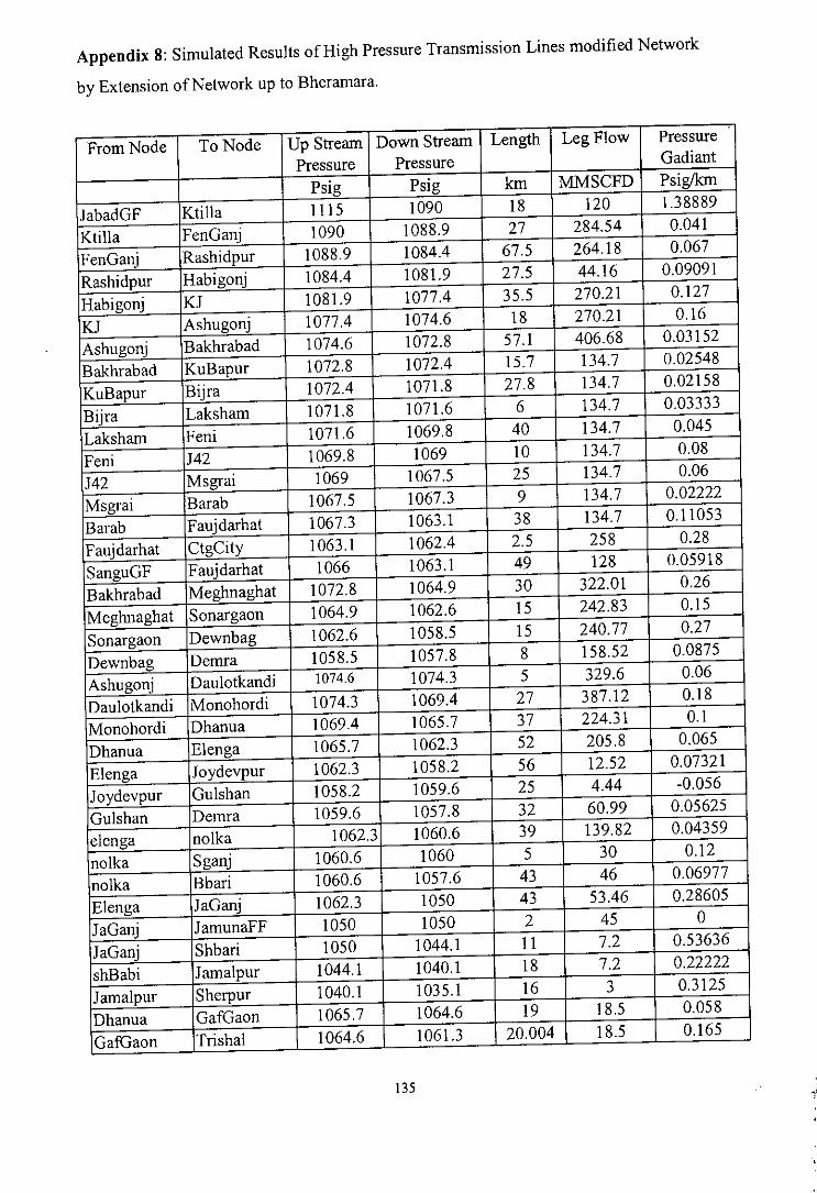
Appendix 8: Simulated Results of High Pressure Transmission Lines modified Network
by Extension of Network up to Bheramara.
From Node To Node Up Stream Down Stream Length Leg Flow Pressure
Pressure Pressure Gadiant
Psig Psig km MMSCFD Psiglkm.
JabadGF Ktilla 1115 1090 18 120 1.38889
Ktilla FenGanj 1090 1088.9 27 284.54 0.041
FenGanj Rashidpur 1088.9 1084.4 67.5 264.18 0.067
Rashidpur Habigonj 1084.4 1081.9 27.5 44.16 0.09091
Habigonj KJ 1081.9 1077.4 35.5 270.21 0.127
KJ Ashugonj 1077.4 1074.6 18 270.21 0.16
Ashugonj Bakhrabad 1074.6 1072.8 57.1 406.68 0.03152
Bakhrabad KuBapur 1072.8 1072.4 15.7 134.7 0.02548
KuBapur Bijra 1072.4 1071.8 27.8 134.7 0.02158
Bijra Laksham 1071.8 1071.6 6 134.7 0.03333
Laksham Feni 1071.6 1069.8 40 134.7 0.045
Feni J42 1069.8 1069 10 134.7 0.08
J42 Msgrai 1069 1067.5 25 134.7 0.06
Msgrai Barab 1067.5 1067.3 9 134.7 0.02222
Barab Faujdarhat 1067.3 1063.1 38 134.7 0.11053
Faujdarhat CtgCity 1063.1 1062.4 2.5 258 0.28
SanguGF Faujdarhat 1066 1063.1 49 128 0.05918
Bakhrabad Meghnaghat 1072.8 1064.9 30 322.01 0.26
Meghnaghat Sonargaon 1064.9 1062.6 15 242.83 0.15
Sonargaon Dewnbag 1062.6 1058.5 15 240.77 0.27
Dewnbag Demra 1058.5 1057.8 8 158.52 0.0875
Ashugonj Daulotkandi 1074.6 1074.3 5 329.6 0.06
Daulotkandi Monohordi 1074.3 1069.4 27 387.12 0.18
Monohordi Dhanua 1069.4 1065.7 37 224.31 0.1
Dhanua Elenga 1065.7 1062.3 52 205.8 0.065
Elenga Joydevpur 1062.3 1058.2 56 12.52 0.07321
Joydevpur Gulshan 1058.2 1059.6 25 4.44 -0.056
Gulshan Demra 1059.6 1057.8 32 60.99 0.05625
elenga nolka 1062.3 1060.6 39 139.82 0.04359
nolka Sganj 1060.6 1060 5 30 0.12
nolka Bbari 1060.6 1057.6 43 46 0.06977
Elenga JaGanj 1062.3 1050 43 53.46 0.28605
JaGanj JamunaFF 1050 1050 2 45 0
JaGanj Shbari 1050 1044.1 11 7.2 0.53636
shBabi Jamalpur 1044.1 1040.1 18 7.2 0.22222
Jamalpur Sherpur 1040.1 1035.1 16 3 0.3125
Dhanua GafGaon 1065.7 1064.6 19 18.5 0.058
GafGaon Trishal 1064.6 1061.3 20.004 18.5 0.165
135

Trisal mymen 1061.3 1057.8 16 18.5 0.21875
Mymen LX 1057.8 1056 8 16.45 0.225
LX Mymenpp 1056 1056 5 14 0
Lx Neykona 1056 1052 32.5 2 0.12308
Monohordi kisGanj 1069.4 1067.6 36 2 0.05
KAI APS 1072.6 1056.5 1.5 175 10.7333
KAI ZiaFF 1072.6 lO72.4 2.4 45 0.08333
Dewnbag hariPP 1060.5 1058.9 1.58 80 1.01266
FenGanj fenpp 1087.9 1068.6 0.5 20 38.6
RashidGF Rashidpur 1084 1082.4 1.9 160 0.84211
HGFI Manifold 1084.6 1084.5 0.006 270 16.67
Manifold ShahjiPP 1083.5 1060.6 2.5 20 9.16
Manifold Habigonj 1083.5 1079.9 1 226.04 3.6
Manifold Katihata 1083.5 1076.8 42 22.98 0.13333
Katihata Manif 1076.8 1074.4 11.5 22.98 0.47826
Manif Ashuganj 1074.4 1074.6 2 98.78 -0.1
N61 Ktilla 1090 1090 0.02 43.33 0
Nlll N61 1083.2 1090 28 41.67 -0.2429
Nlll Kuchai 1083.2 1088.9 2.082 66.67 -2.7378
Kuchai Sylhet 1088.9 976.47 0.03 76 3747.67
HariGF Kuchai 1063.3 1088.9 12 6 -2.1333
SaldaGf Bakhrabad 1019 1072.8 35 30 -1.5371
MeghnaGF Bakhrabad 1028.8 1072.8 28 20 -1.5714
TitasGf Bbaria 1100 1087.2 1 300 12.8
Bbaria TNI 1087.2 1086 1 150.57 1.2
Bbaria TN2 1087.2 1086.4 1 147.39 0.8
TNI KAI 1086 1072.6 14.1 150.57 0.95035
KAI TN3 1072.6 1071.7 7 46.22 0.12857
TN3 Nars 1071.7 1064.2 30 46.22 0.25
TN2 Daulot# 1086.4 1074.4 16 147.39 0.75
Daulot# TN4 1074.4 1064.5 29 89.88 0.34138
TN4 Nars 1064.5 1064.2 1 89.88 0.3
Nars Tarabo 1064.2 1063.4 20 8.09 0.04
Tarabo Demra 1063.4 1057.8 12 4.2 0.46667
Nars Tarabo# 1064.2 1063.4 40 50.57 0.02
Tarabo# ShiddPP 1063.4 1063.1 5 54.47 0.06
ShiddPP ShiddPS 1063.1 1063.1 0.0003 52 0
ShiddPP N76 1063.1 1062.2 10 1.08 0.09
N76 Demra 1062.2 1057.8 10 1.08 0.44
Nras Ghorasal 1064.2 1058.4 8.4 254.62 0.69048
Ghorasal GhoraPP 1058.4 899.7 0.4 166 396.75
Ghorasal GhoraFF 1058.4 1056.5 8.4 61.6 0.22619
GhoraFF DGhoraFF 1056.5 1056.5 0.0003 40 0
GhoraFF PalashFF 1056.5 1056.4 0.8 20 0.125
Monohordi Nars 1069.4 1064.2 32 158.71 0.225
Daulot# Daulotkandi 1074.4 1074.3 0.1 57.5 1
t36

BelaboGF Nars 1090.5 1064.2 13 20 2.0230769
Rashidpur NI08 1084.4 1082.8 10 480.03 0.16
NI08 NI09 1082.8 1080.1 30 480.03 0.09
NI09 Ashugonj 1080.1 1074.6 37 570.03 0.15
BibyanaGF Rashidpur 1091.1 1084.4 30 100 0.223
KatiGF NI09 1085.6 1078 1 90 7.6
Appendix 9: Simulated Results of High Pressure Transmission Lines Extension of
Network up to Khulna without any Modification
Source/ Delivery Name Source/ Deliverv. Pressure, Psig Flow Rate, MMSCFD
Titas gas field Source 1114.3 300
Habigoni Gas field Source 1106.1 270
Rashidpur Gas Field Source 1091.7 250
Jalalabad Gas Field Source 1112.3 120
Sangu Gas Field Source 1004.7 160
Narshindi Gas Field Source 956.39 15
Meghna Gas Field Source 1038.5 15
Salda Gas field Source 1017.6 15
Kailashtilla(MSTE) gas Field Source 1090 200
Kailashtilla(Sillica) gas field Source 1089.9 60
Beanibazar Gas Field Source 1090.7 30
Haripur Gas Field Source 1088.9 4
Bibyana Gas Field Source 1181.3 300
Kati (Titas) Source 1097.9 40
Bakhrabad Gas Field Source 1004.9 0.005
APS Sink 947.75 140
GhoraPP Sink 863.38 180
HaripPP Sink 938.82 95
MvmenPP Sink 906.98 18
ShiddPP Sink 939.04 52
FenPP Sink 1088.9 20
ShahiPP Sink 1089.5 36
ZiaFF Sink 1002 56
GhoraFF Sink 932.84 40
PalashFF Sink 931.84 20
JamuanaFF Sink 828.01 45
Joydevpur Sink 932.81 9
Gulshan Sink 932.87 80
Shiraigoni Sink 824.87 40
Baghabari Sink 824.72 100
Ctgcity Sink 982.9 300
Sylhet Sink 926.24 80
Demra Sink 938.85 110
Khulna Sink 740.55 100
137

!EP-PP .BheraPP
SinkSink
812.2805.13
1070
Appendix 10: Simulated Results of High Pressure Transmission Lines Extension of
Network up to Khulna with A-D Loop Line.
From Node .' To Node' , Up Stream DoWn Stream' Length ~Leg Flow~ ::.:Ptessure;:'. . -. . . , GadiantPressure Pressure <.
Psig . Psig . kID .•.. MMSCFD Psiglkm
JabadGF Ktilla 1112.3 1090 18 120 1.23889
Ktilla FenGanj 1090 1088.6 27 339.29 0.052
FenGanj Rashidpur 1088.6 1083.9 67.5 319.45 0.07
Rashidpur Habigonj 1083.9 1080.8 27.5 140.42 0.11273
Habigonj KJ 1080.8 1075.2 35.5 346.79 0.158
KJ Ashugonj 1075.2 1070.9 18 346.79 0.239
Ashugonj Bakhrabad 1070.9 1068.9 57.1 481.5 0.03503
Bakhrabad KuBapur 1068.9 1068.3 15.7 144.04 0.03822
KuBapur Bijra 1068.3 1067.1 27.8 144.04 0.04317
Bijra Laksham 1067.1 1066.9 6 144.04 0.03333
Laksham Feni 1066.9 1065.1 40 144.04 0.045
Feni J42 1065.1 1064.4 10 144.04 0.07
J42 Msgrai 1064.4 1062.2 25 144.04 0.088
Msgrai Barab 1062.2 1061.3 9 144.04 0.1
Barab Faujdarhat 1061.3 1056.6 38 144.04 0.12368
Faujdarhat CtgCity 1056.6 1056.6 2.5 300 0
SanguGF Faujdarhat 1060.6 1056.6 49 160 0.08163
Bakhrabad Meghnaghat 1068.9 1062.6 30 367.47 0.21
Meghnaghat Sonargaon 1062.6 1060 15 260.39 0.17333
Sonargaon Dewnbag 1060 1057.9 15 258.35 0.14
Dewnbag Demra 1057.9 1057.2 8 161.47 0.0875
Ashugonj Daulotkandi 1070.9 1070.7 5 190.5 0.04
Daulotkandi Monohordi 1070.7 1069.2 27 246.76 0.05556
Monohordi Dhanua 1069.2 1066.1 37 47.81 0.08378
Dhanua Elenga 1066.1 1058 52 394.16 0.15577
Elenga Joydevpur 1058 1052.5 56 14.88 0.09821
Joydevpur Gulshan 1052.5 1050.4 25 0.466 0.084
Gulshan Demra 1050.4 1057.2 32 81.15 -0.2125
elenga nolka 1058 1054 39 326.27 0.10256
nolka Sganj 1054 1053.9 5 40 0.02
nolka Bbari 1054 1049.8 43 100 0.09767
Elenga JaGanj 1058 1045.7 43 53.02 0.28605
JaGanj JamunaFF 1045.7 1045.7 2 45 0
JaGanj Shbari 1045.7 1039.8 11 7.14 0.53636
138 ••
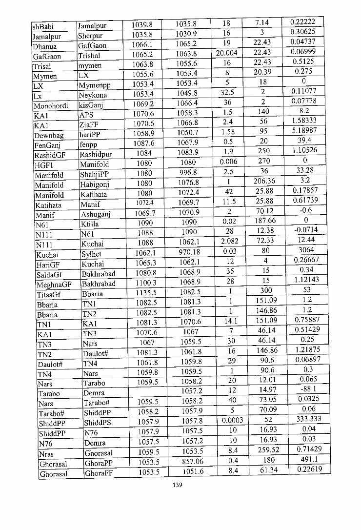
shBabi Jamalpur 1039.8 1035.8 18 7.14 0.22222
Jamalpur Sherpur 1035.8 1030.9 16 3 0.30625
Dhanua GafGaon 1066.1 1065.2 19 22.43 0.04737
GafGaon Trishal 1065.2 1063.8 20.004 22.43 0.06999
Trisal mymen 1063.8 1055.6 16 22.43 0.5125
Mymen LX 1055.6 1053.4 8 20.39 0.275
LX Mymenpp 1053.4 1053.4 5 18 0
Lx Neykona 1053.4 1049.8 32.5 2 0.11077
Monohordi kisGanj 1069.2 1066.4 36 2 0.07778
KAI APS 1070.6 1058.3 1.5 140 8.2
KAI ZiaFF 1070.6 1066.8 2.4 56 1.58333
Dewnbag hariPP 1058.9 1050.7 1.58 95 5.18987
FenGanj fenpp 1087.6 1067.9 0.5 20 39.4
RashidGF Rashidpur 1084 1083.9 1.9 250 1.10526
HGFI Manifold 1080 1080 0.006 270 0
Manifold ShahjiPP 1080 996.8 2.5 36 33.28
Manifold Habigonj 1080 1076.8 1 206.36 3.2
Manifold Katihata 1080 1072.4 42 25.88 0.17857
Katihata Manif 1072.4 1069.7 11.5 25.88 0.61739
Manif Ashuganj 1069.7 1070.9 2 70.12 -0.6
N61 Ktilla 1090 1090 0.02 187.66 0
N1l1 N61 1088 1090 28 12.38 -0.0714
Nlll Kuchai 1088 1062.1 2.082 72.33 12.44
Kuchai Sylhet 1062.1 970.18 0.03 80 3064
HariGF Kuchai 1065.3 1062.1 12 4 0.26667
SaldaGf Bakhrabad 1080.8 1068.9 35 15 0.34
MeghnaGF Bakhrabad 1100.3 1068.9 28 15 1.12143
TitasGf Bbaria 1135.5 1082.5 1 300 53
Bbaria TNI 1082.5 1081.3 1 151.09 1.2
Bbaria TN2 1082.5 1081.3 1 146.86 1.2
TNI KAI 1081.3 1070.6 14.1 151.09 0.75887
KAI TN3 1070.6 1067 7 46.14 0.51429
TN3 Nars 1067 1059.5 30 46.14 0.25
TN2 Daulot# 1081.3 1061.8 16 146.86 1.21875
Daulot# TN4 1061.8 1059.8 29 90.6 0.06897
TN4 Nars 1059.8 1059.5 1 90.6 0.3
Nars Tarabo 1059.5 1058.2 20 12.01 0.065
Tarabo Demra 1057.2 12 14.97 -88.1
Nars Tarabo# 1059.5 1058.2 40 73.05 0.0325
Tarabo# ShiddPP 1058.2 1057.9 5 70.09 0.06
ShiddPP ShiddPS 1057.9 1057.8 0.0003 52 333.333
ShiddPP N76 1057.9 1057.5 10 16.93 0.04
N76 Demra 1057.5 1057.2 10 16.93 0.03
Nras Ghorasal 1059.5 1053.5 8.4 259.52 0.71429
Ghorasal GhoraPP 1053.5 857.06 0.4 180 491.1
Ghorasal GhoraFF 1053.5 1051.6 8.4 61.34 0.22619
139
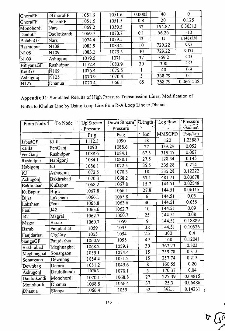
GhoraFF DGhoraFF 1051.6 1051.6 0.0003 40 0
GhoraFF PalashFF 1051.6 1051.5 0.8 20 0.125
Monohordi Nars 1069.2 1059.5 32 194.87 0.30313
Daulot# Daulotkandi 1069.7 1070.7 0.1 56.26 -10
BelaboGF Nars 1074.4 1059.5 13 15 1.1461538
Rashidpur NI08 1083.9 1083.2 10 729.22 0.07
NI08 NI09 1083.2 1079.5 30 729.22 O. t23
NI09 Ashugonj 1079.5 1071 37 769.2 0.23
BibyanaGF Rashidpur 1172.4 1083.9 30 300 2.95
KatiGF NI09 1076.4 1075.5 I 40 0.9
Ashugonj NI25 1070.9 1070.4 5 368.79 0.1
NI25 Dhanua 1070.4 1066.1 65 368.79 0.0661538
Appendix 11: Simulated Results of High Pressure Transmission Lines, Modification of
Nolka to Khulna Line by Using Loop Line from R-A Loop Line to Dhanua
From Node' "To Node .' 1,JpStr.earn' Down Stream" :Length; ~Legflow' " Pressure", ' Pressure . Pressure ,~ " ; Gaai;rnt. . .
Psig Psig . Ian MMSCFD Psiglkm
JabadGF Ktilla 1112.3 1090 18 120 1.23889
Ktilla FenGanj 1090 1088.6 27 339.29 0.052
FenGanj Rashidpur 1088.6 1084.1 67.5 319.45 0.067
Rashidpur Habigonj 1084.1 1080.1 27.5 128.34 0.145
Habigonj KJ 1080.1 1072.5 35.5 335.28 0.214
KJ Ashugonj 1072.5 1070.3 18 335.28 0.12222
Ashugonj Bakhrabad 1070.3 1068.2 57.1 481.71 0.03678
Bakhrabad KuBapur 1068.2 1067.8 15.7 144.51 0.02548
KuBapur Bijra 1067.8 1066.1 27.8 144.51 0.06115
Bijra Laksham 1066.1 1065.8 6 144.51 0.05
Laksham Feni 1065.8 1063.6 40 144.51 0.055
Feni J42 1063.6 1062.7 10 144.51 0.09
J42 Msgrai 1062.7 1060.7 25 144.51 0.08
Msgrai Barab 1060.7 1059 9 144.51 0.18889
Barab Faujdarhat 1059 1055 38 144.51 0.10526
Faujdarhat CtgCity lOSS 1054 2.5 300 0.4
SanguGF Faujdarhat 1060.9 lOSS 49 160 0.12041
Bakhrabad Meghnaghat 1068.2 1059.1 30 367.23 0.303
Meghnaghat Sonargaon 1059.1 1054.4 IS 259.78 0.313
Sonargaon Dewnbag 1054.4 1051.2 IS 257.74 0.213
Dewnbag Demra 1051.2 1049.6 8 160.55 0.20
Ashugonj Daulotkandi 1070.3 1070.1 5 170.37 0.04
Daulotkandi Monohordi 1070.1 . 1068.8 27 227.39 0.04815
Monohordi Dhanua 1068.8 1066.4 37 25.3 0.06486
Dhanua Elenga 1066.4 1059 52 392.1 0.14231
140

Elenga Joydevpur 1059 1053 56 15.06 0.10714
Joydevpur Gulshan 1053 1052.8 25 0.649 0.008
Gulshan Demra 1052.8 1049.6 32 81.22 0.1
elenga nolka 1059 1054.9 39 324.33 0.10513
nolka Sganj 1054.9 1054.8 5 40 0.02
nolka Bbari 1054.9 1050.7 43 100 0.09767
Elenga JaGanj 1059 1046.7 43 52.71 0.28605
JaGanj JamunaFF 1046.7 1046.7 2 45 0
JaGanj Shbari 1046.7 1040.8 11 7.09 0.53636
shBabi Jamalpur 1040.8 1036.7 18 7.09 0.22778
Jamalpur Sherpur 1036.7 1030.9 16 3 0.3625
Dhanua GafGaon 1066.4 1066.1 19 22.3 0.01579
GafGaon Trishal 1066.1 1060.8 20.004 22.3 0.26495
Trisal mymen 1060.8 1056.5 16 22.3 0.26875
Mymen LX 1056.5 1054.3 8 20.27 0.275
LX Mymenpp 1054.3 1054.3 5 18 0
Lx Neykona 1054.3 1050.7 32.5 2 0.11077
Monohordi kisGanj 1068.8 1067 36 2 0.05
KAI APS 1071 1058.6 1.5 140 8.26667
KAI ZiaFF 1071 1067.2 2.4 56 1.58333
Dewnbag hariPP 1053.2 1051.1 1.58 95 1.32911
FenGanj fenpp 1087.6 1067.9 0.5 20 39.4
RashidGF Rashidpur 1082 1081.1 1.9 250 0.47368
HGFI Manifold 1080.1 1080.1 0.006 270 0
Manifold ShahjiPP 1080.1 996.9 2.5 36 33.28
Manifold Habigonj 1080.1 1077.9 1 206.93 2.2
Manifold Katihata 1080.1 1072.7 42 25.31 0.17619
Katihata Manif 1072.7 1070.1 11.5 25.31 0.22609
Manif Ashuganj 1070.1 1070.3 2 70.26 -0.1
N61 Ktilla 1090 1090 0.02 187.66 0
Nlll N61 1088 1090 28 12.33 -0.0714
Nlll Kuchai 1088 1062.4 2.082 72.33 12.2959
Kuchai Sylhet 1062.4 970.18 0.03 80 3074
HariGF Kuchai 1065.3 1062.4 12 4 0.24167
SaldaGf Bakhrabad 1081.1 1068.2 35 15 0.36857
MeghnaGF Bakhrabad 1100.7 1068.2 28 15 1.16071
TitasGf Bbaria 1133.9 1082.9 1 300 51
Bbaria TNI 1082.9 1081.7 1 151.21 1.2
Bbaria TN2 1082.9 1082.1 1 146.74 0.8
TNI KAI 1081.7 1071 14.1 151.21 0.75887
KAI TN3 1071 1067.4 7 45.64 0.51429
TN3 Nars 1067.4 1060 30 45.64 0.24667
TN2 Daulot# 1082.1 1070.1 16 146.74 0.75
Daulot# TN4 1070.1 1060.2 29 89.72 0.34138
TN4 Nars 1060.2 1060 1 89.72 0.2
Nars Tarabo 1060 1058.6 20 12.21 0.07
141

Tarabo Demra 1058.6 1049.6 12 15.5 0.75
Nars Tarabo# 1060 1058.6 40 74.96 0.035
Tarabo# ShiddPP 1058.6 1058.3 5 70.97 0.06
ShiddPP ShiddPS 1058.3 1058.3 0.0003 52 0
ShiddPP N76 1058.3 1057.6 10 17.73 0.07
N76 Demra 1057.6 1049.6 10 17.73 0.8
Nras Ghorasal 1060 1054 8.4 259.84 0.71429
Ghorasa1 GhoraPP 1054 857.54 0.4 180 491.15
Ghorasal GhoraFF 1054 1052.1 8.4 61.44 0.22619
GhoraFF DGhoraFF 1052.1 1052.1 0.0003 40 0
GhoraFF PalashFF 1052.1 1052 0.8 20 0.125
Monohordi Nars 1068.8 1060 32 198 0.275
Daulot# Daulotkandi 1070.1 1070.1 0.1 57.02 0
BelaboGF Nars 1074.9 1060 13 15 1.14615
Rashidpur N108 1084.1 1081.8 10 741.3 0.23
N108 N109 1081.8 1075.9 30 741.3 0.197
N109 Ashugonj 1075.9 1070.7 37 392.18 0.1405405
BibyanaGF Rashidpur 1172.4 1081.1 30 300 3.0433333
KatiGF N109 1078 1075.9 1 40 2.1
N110 Dhanua 1070.7 1066.4 69 188.07 0.06232
142

Appendix 12: Simulated Results of High Pressure Transmission Lines modified
Network by using Compressor Station at Monohordi.
Source/ Delivery Name Source/ Delivery Pressure, Psig Flow Rate, MMSCFD
Titas gas field Source 1106.3 300
Habigonj Gas field Source 1103.7 270
Rashidpur Gas Field Source 1090.8 250
Jalalabad Gas Field Source 1112.3 120
Sangu Gas Field Source 1010 160
Narshindi Gas Field Source 952.47 15
Meghna Gas Field Source 1043.6 15
Sa1daGas field Source 1022.8 15
Kailashtilla(MSTE) gas Field Source 1090 200
Kailashtilla(Sillica) gas field Source 1089.9 60
Beanibazar Gas Field Source 1090.7 30
Haripur Gas Field Source 1088.9 4
Bibyana Gas Field Source 1181.4 300
Kati (Titas) Source 1059.2 40
Bakhrabad Gas Field Source 1012.2 0.005
APS Sink 952.71 140
GhoraPP Sink 857.39 180
HaripPP Sink 925.51 95
MymenPP Sink 957.64 18
ShiddPP Sink 935.27 52
FenPP Sink 1088.9 20
ShahiPP Sink 1086.9 36
ZiaFF Sink 1005.8 56
GhoraFF Sink 926.31 40
PalashFF Sink 925.21 20
JamuanaFF Sink 881.5 45
Joydevpur Sink 923.92 9
Gulshan Sink 925.09 80
Shirajgonj Sink 853.67 40
Baghabari Sink 853.5 100
Ctgcity Sink 1000.1 300
Sylhet Sink 926.37 80
Demra Sink 925.46 110
Khulna Sink 975.1 100
EP-PP Sink 990 10
BheraPP Sink 988 70
MeghPP Sink 941.11 105
143

NOMENCLATURE
u= Internal energy, ft-Ibr/ Ibm
V = fluid velocity, ft / sec
z = elevation above a given datum place, ft
p = pressure, Ibr / ft2
V = volume of a unit mass of the fluid, ftJ / Ibm
Ws = shaft work done by the fluid on the surroundings, ft-lbr / Ibm
g = gravitational acceleration, ft / sec2
go= conversion factor relating mass and weight
h = specific fluid enthalpy, ft-Ibr / Ibm
T = temperature, oR
s = specific fluid entropy, ft-Ibr / Ibm
pmax= maximum allowable internal pressure, psig
t = pipe thickness, inc = sum of mechanical allowances, corrosion, erosion, etc., in.
S = allowable stress for the pipe material, psi
E = longitudinal weld joint factor, in.
do= outside diameter of the pipe, in.
Y = temperature de-rating factor
ve= erosional velocity, ft/sec
p = Fluid density, Ibm/ftJ
C = a constant ranging between 75 and 150
(qe)se= gas flow rate for onset of erosion, Mscfd
d = diameter of the pipe, ft
p = flowing pressure, PSIA
R = gas constant
Z = gas compressibility factor at pressure p and temperature T
qsc= gas flow rate measured at saturated conditions, Mscfd
psc= pressure at saturated conditions, psia
Tse= temperature at saturated conditions, OR
PI = upstream pressure, psia
P2= downstream pressure, psi a
144

Yg = gas gravity (air = I basis)
Zav= average gas compressibility factor
f = Moody friction factor
L = length of the pipe, ft
dch= choke diameter, in
T 1 = inlet temperature, oRz,~ mole fraction of vapor (gas) in the gas-liquid flow-stream
cp= fluid specific heat at constant pressure, Btu/Ibm-oF
)1d = Joule- Thomson coefficient, ft2-°F/lbr
m = mass flow rate, Ibm/sec
Q = phase-transition heat, Btu/Ibm
k = thermal conductivity, Btu/ft-sec-oF
do= outlet pipe diameter, ft
Ts = temperature of the soil or surroundings,OF
kg = Productivity index of the reservoir
F = a transmission factor that is based on the flow regime and other variables,
F=4Iog(3.7dlK), K is the relative roughness of the pipe
Pm= the mean pressure in the pipeline
Zm= the super compressibility factor at the mean pressure
H = the change in elevation of the pipeline between inlet and outlet
r
145 \" !(-,'->
\'.

REFERENCES1. Quader, A.K.M.A, and E. Gomes, "An Exploratory Review of Bangladesh Gas
Sector: Latest Evidence and Areas of Future Research", Centre for Policy
Dialogue, January 24 (2002).2. Saleque, Kh. A., Growth of Natural Gas Sector in Bangladesh - Issues and
Options, Seventh National Convention of Chemical Engineers, December 12
(1998).3. Ejaz, S., Production System Analysis of the Titas Gas Field, M.Sc. Thesis,
Chemical Engineering Department, BUET, Dhaka, 1999.
4. Khan, M.A.A. and Imamududdin, M., Mid Term Gas Demand - Supply Scenario
and Gas Reserves of Bangladesh, Presented at the 2nd Petroleum Engineering
Symposium 1999,24-25 May (1999).
5. Quader, A.K.M.A., Utilization of Natural Gas in Bangladesh and its Future,
Indian Chemical Engineering Congress, Calcutta, December 18-21, 2000.
6. Kennedy J. L., "Oil and Gas Pipeline Fundamentals", Second Edition PennWell
Books, Tulsa, Oklahoma, 1993.
7. Daily Production Reports, GTCL 2000.
8. Petrobangla MIS Division, Petro-center, Dhaka, 2002
9. Gas System Development Plan (Final report), Asian Development Bank, T.A.N°
2024 - BAN, Volume-I, July1996.
10. System Planning Department, PDB, Dhaka, 2000.
11. CLD Department, Titas Gas Transmission and Distribution Co. Ltd., Kawran
Bazar, Dhaka, 2001.12. Rashidpur-Ashugonj Gas Transmission Loop Line Project, Request for Proposal
(REP), Gas Transmission Company Ltd. (GTCL).
13. PIPESIM Operating Manual, Revision (March '1998), Baker Jardine and
Associates Limited, London, England.
14. Monthly Production Reports Petrobangla, Petro-center, Dhaka, 1999,2001.
15. Planning Department, Jalalabad Gas Transmission and Distribution System
Limited, Sylhet, 2000.
16. Planning Department, Gas Transmission and Distribution Company Limited,
Dhaka, 2000.
146
(/"."
(i
~,

17. Kumer S., " Gas Production Engineering", volume 4, Gulf Publishing company,
Houston, Texas, 1987.
18. Perry, R. H. and Cecil, H. c., Chemical Engineers' Hand book, fifth edition,
McGRA W-HlLL KOGAKUSHA, LTD., Tokyo, 1963.
19. Economides, MJ., A.D. Hill, "Petroleum Production Systems".
20. Beggs H. D., " Gas Production Operations", OGCI Publications, Tulsa,
Oklahoma, 1984.21. Gas Engineers Handbook, Fuel Gas Engineering Practice, Industrial Press Inc.,
New York, 1969.
147
r'