Analysis techniques for subdivision schemes Joe Warren Rice University

Analysis techniques for subdivision schemes

Joe Warren

Rice University

A teaser for subdivision gurus

Consider the basis function Consider the basis function n(t)n(t) for the for the standard, four point interpolatory scheme.standard, four point interpolatory scheme.

Note this function is Note this function is notnot piecewise polynomial! piecewise polynomial!What is the exact value of What is the exact value of n(n(⅓⅓)) as a rational as a rational

number?number?

01 1 223 3

Choosing a modeling technology

Many possibilities – points, polygons, algebraics, Many possibilities – points, polygons, algebraics, implicits, NURBS, subdivision surfacesimplicits, NURBS, subdivision surfaces

Choice based on various factors Choice based on various factors Ease of useEase of use Expressiveness Expressiveness Computational efficiencyComputational efficiency Analysis techniquesAnalysis techniques

Subdivision surfaces – strong on first three points, Subdivision surfaces – strong on first three points, perceived as weak on lastperceived as weak on last

Typical analysis problems

1.1. Determine the smoothness of a given Determine the smoothness of a given curve/surface scheme.curve/surface scheme.

2.2. Perform exact evaluation of positions, Perform exact evaluation of positions, tangents and inner products for a given tangents and inner products for a given curve/surface scheme.curve/surface scheme.

3.3. Interpolate a networks of curves using a Interpolate a networks of curves using a given surface scheme.given surface scheme.

Analysis of subdivision schemes using linear algebra

Convergence/smoothness analysis for subdivision Convergence/smoothness analysis for subdivision schemesschemes

D S = T DD S = T D Exact computation of values, derivatives and inner Exact computation of values, derivatives and inner

products for subdivision schemesproducts for subdivision schemesN S = NN S = N

SSTT E S = E E S = E Interpolation of curves using subdivision schemesInterpolation of curves using subdivision schemes

M S = C MM S = C M

Example: Cubic subdivision

Add new vertices between pairs of consecutive vertices, repositioned via rules

81

81

43

21

21

Example: Catmull-Clark subdivision

16

1

8

3

16

1

16

1

8

3

16

1

4

1

4

1

4

1

4

1

16

9

n8

3

n8

3

n8

3

n8

3

n16

1

n16

1

n16

1

n16

1

Subdivision as linear algebra Express positions of vertices of coarse and Express positions of vertices of coarse and

fine mesh as column vectors fine mesh as column vectors ppkk and and ppk+1k+1

Construct Construct subdivision matrixsubdivision matrix SS whose rows whose rows correspond to rules for schemecorrespond to rules for scheme

Relate vectors via the subdivision relationRelate vectors via the subdivision relation

ppk+1k+1 = = S pS pkk

Apply linear algebra to Apply linear algebra to SS to analyze and to analyze and manipulate the schememanipulate the scheme

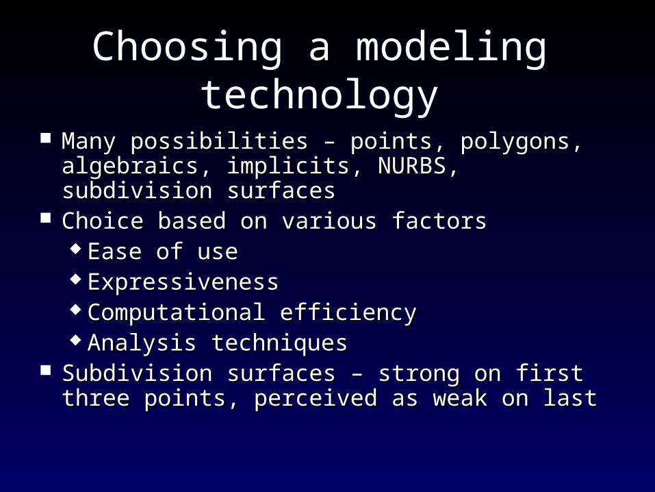
Subdivision matrix for cubics

Rows of subdivision matrix S alternate between rules and

Consider only 5x5 sub-matrix centered at fixed mesh vertex

.......

.81

43

8100.

.021

2100.

.081

43

810.

.0021

210.

.0081

43

81.

.......

S

81

43

81 2

12

1

Part I – Smoothness analysis

Given a schemeGiven a scheme,, are the limit meshes produced are the limit meshes produced by the scheme by the scheme CCnn continuous? continuous?

Observe that Observe that ppkk is related to is related to pp00 via via

ppkk = = SSkk p p00

Compute diagonal matrix Compute diagonal matrix ΛΛ of eigenvalues of eigenvalues and matrix Z of right eigenvectors satisfyingand matrix Z of right eigenvectors satisfying

S=ZΛ ZS=ZΛ Z-1-1

Right eigenvectors & polynomials

TheoremTheorem: If scheme is : If scheme is CCnn continuous, let continuous, let ZZpp

denoted those right eigenvectors of denoted those right eigenvectors of Z Z with with eigenvalues (½)eigenvalues (½)jj where where 0 ≤ j ≤ n.0 ≤ j ≤ n.

Then the right eigenvectors of Then the right eigenvectors of ZZpp converge to converge to

polynomials of degree at most polynomials of degree at most n.n.

CC22 cubic example:cubic example:

38

32

31

32

38

21

11

01

11

21

pZ

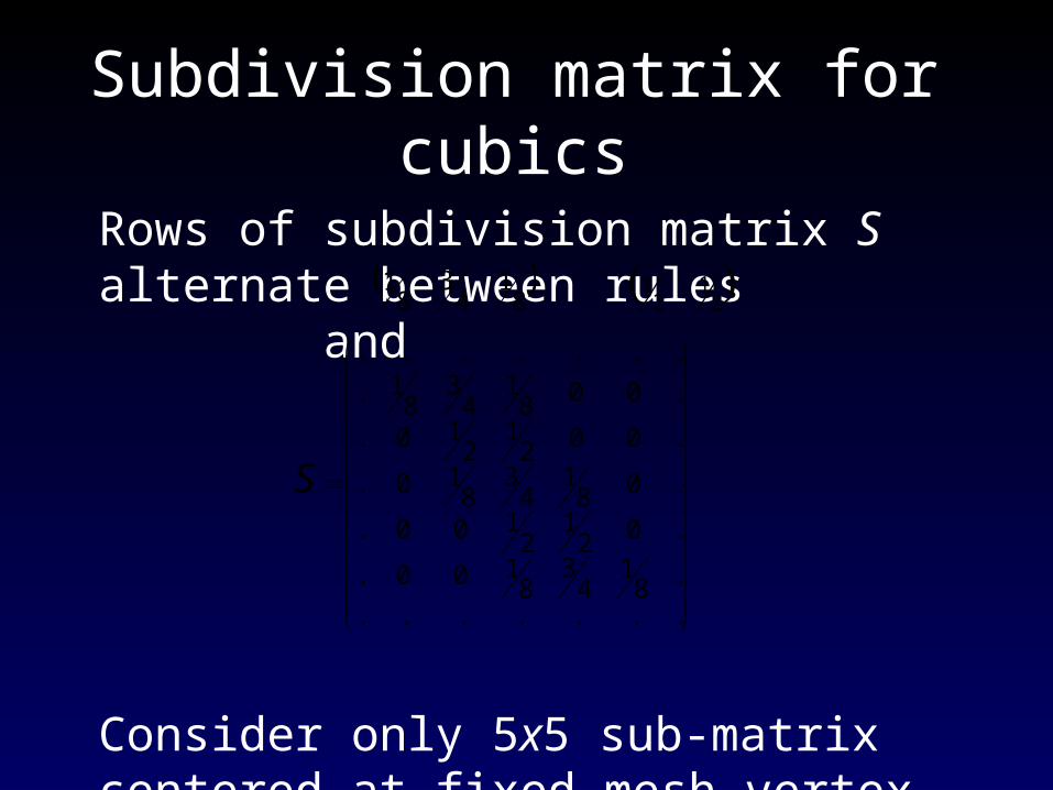
Smoothness condition

Build difference matrix Build difference matrix DD that annihilates that annihilates ZZpp

D ZD Zp p = 0= 0 Construct matrix Construct matrix TT that satisfies relation that satisfies relation

(2(2nn D) S = T D D) S = T D TT is subdivision matrix for differences is subdivision matrix for differences D pD pkk

(2(2nn D) p D) pk+1k+1 = T D p = T D pkk

TheoremTheorem: If there exists : If there exists k>0k>0 with with║T║Tkk║║∞∞< < 1, 1, the limit meshes for the scheme are the limit meshes for the scheme are CCnn

Smoothness for cubic splines

Form difference matrix Form difference matrix D D as nullspace of as nullspace of ZZpp

Compute subdivision matrix Compute subdivision matrix TT for differences for differences

Observe that Observe that ║T║║T║∞∞=½=½ so scheme is so scheme is CC22

13310

01331D

21

21

0

0T

Non-uniform subdivision schemes

Tri/quad subdivision - mesh of triangles/quadsTri/quad subdivision - mesh of triangles/quads

Methods - Loop/Stam, LevinMethods - Loop/Stam, Levin22, Schaefer/Warren, Schaefer/Warren

C2 analysis for tri/quad schemes

Construct matrix Construct matrix SS for tri/quad interface for tri/quad interface Compute Compute ZZpp, D, , D, and and TT from from SS Attempt to find Attempt to find k>0k>0 such that such that ║T║Tkk║║∞∞<1<1

Problems:Problems: D D and and TT are not uniquely determined are not uniquely determined Bounding Bounding ║T║Tkk║║∞∞ is difficult since number of distinct is difficult since number of distinct

rows in rows in TTkk grows exponentiallygrows exponentially

For non-uniform schemes, assembling these rows is a For non-uniform schemes, assembling these rows is a tricky computationtricky computation

Simpler smoothness test (Levin2)

Construct finite sub-matrices Construct finite sub-matrices SS00 and and SS11 of of

matrix matrix SS centered along tri/quad interface centered along tri/quad interface

S0

Simpler smoothness test (Levin2)

Construct finite sub-matrices Construct finite sub-matrices SS00 and and SS11 of of

matrix matrix SS centered along tri/quad interface centered along tri/quad interface

S1

Joint spectral radius condition

Compute finite subdivision matrices Compute finite subdivision matrices TT00 and and TT11

4D S4D S00 = T = T00 D D

4D S4D S11 = T = T11 D D

Theorem:Theorem: If there exists a If there exists a k>0 k>0 such that such that

║║TTe1e1TTe2e2…T…Tek ek ║║∞∞<1<1

for all for all eeii {0,1} {0,1}, the scheme is , the scheme is CC22

Part II – Exact evaluation

Problem: Given a scheme, compute exact Problem: Given a scheme, compute exact values for positions and tangents of limit values for positions and tangents of limit mesh at arbitrary locations.mesh at arbitrary locations.

Problem: Given a scheme, compute the exact Problem: Given a scheme, compute the exact value for inner products of functions defined value for inner products of functions defined via the scheme.via the scheme.

Exact position on limit mesh

Treat mesh as being parameterized by Treat mesh as being parameterized by tt Compute limit position of mesh at arbitrary Compute limit position of mesh at arbitrary tt For piecewise polynomial schemes, blossom For piecewise polynomial schemes, blossom

right eigenvectors (Stam)right eigenvectors (Stam) For non-polynomial schemes, develop For non-polynomial schemes, develop

method to evaluate mesh at method to evaluate mesh at rationalrational pts pts t=i/jt=i/j Get tangents by evaluating difference schemeGet tangents by evaluating difference scheme

Two-scale relation

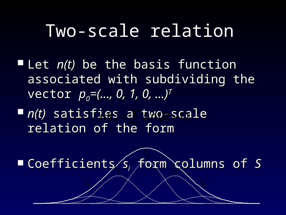
Let Let n(t)n(t) be the basis function associated with be the basis function associated with subdividing the vector subdividing the vector pp00=(…, 0, 1, 0, …)=(…, 0, 1, 0, …)TT

n(t)n(t) satisfies a two-scale relation of the form satisfies a two-scale relation of the form

Coefficients Coefficients ssii form columns of form columns of SS4

3

21

21

81

81

)2()( itnstn i

Exact evaluation at rational pts

KeyKey: To compute : To compute n(i/j), n(i/j), treat value of treat value of n(t) n(t) on on the integer grid as being unknownsthe integer grid as being unknowns

Use two-scale relation to setup system of Use two-scale relation to setup system of equations relating these unknownsequations relating these unknowns

Solve equations to generate exact valuesSolve equations to generate exact values Solution is dominant left eigenvector of Solution is dominant left eigenvector of

upsampled S generated using power methodupsampled S generated using power method

j1

Exact values of n(i/3) for cubics

Examples of equations generated by two-scale Examples of equations generated by two-scale

Exact values from Exact values from –2–2 to 2 to 2

)()()()(

)()()()()(

35

43

31

21

32

81

32

35

21

32

43

31

21

34

81

31

nnnn

nnnnn

01 1 22

00 1621

814

61

2710

5431

32

5431

2710

61

814

1621

Values of n(i/3) for 4 pt scheme

Four point scheme – non-polynomial scheme Four point scheme – non-polynomial scheme

Exact values for Exact values for –3–3 to to 00

1 169

169

161

161

01 1 223 3

1000 55894240

55892000

5589410

5589256

558916

55891

Exact valuation of inner products

Given Given pp00 and and qq00, compute inner product , compute inner product

where where p(t)=pp(t)=p∞∞ and and q(t)=qq(t)=q∞∞

Applications include fitting, fairing, mass Applications include fitting, fairing, mass propertiesproperties

Previous work – compute using polynomial rep Previous work – compute using polynomial rep with infinite sums at extraordinary vertices with infinite sums at extraordinary vertices (Peters, Reif)(Peters, Reif)

dttqtp )()(

A relation for inner products

Define inner product matrix Define inner product matrix E E satisfyingsatisfying

Express Express p(t) p(t) and and q(t)q(t) as combinations of as combinations of n(t-n(t-i)i)

Express as sum of inner Express as sum of inner products of translated products of translated n(2t)n(2t) via two-scale eqs via two-scale eqs

SSTT E S = 2 E E S = 2 E

00)()( qEpdttqtp T( ) ( )n t i n t j dt

( ) ( )ijE n t i n t j dt

Enclosed area as an inner product

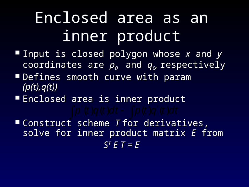
Input is closed polygon whose Input is closed polygon whose xx and and yy coordinates are coordinates are pp00 and and qq00, , respectivelyrespectively

Defines smooth curve with param Defines smooth curve with param (p(t),q(t))(p(t),q(t)) Enclosed area is inner productEnclosed area is inner product

Construct scheme Construct scheme T T for derivatives, solve for for derivatives, solve for inner product matrix inner product matrix EE from from

SSTT E T = E E T = E

dttqtpdttqtp )()()()(

Enclosed area for 4 point curves

Rows of inner product matrix Rows of inner product matrix EE are shifts of are shifts of

Inscribe base polygon in unit circle - graph areaInscribe base polygon in unit circle - graph area

10 12 14 16 18 20

3.115

3.125

3.13

3.135

3.14

6652801

103954

73920481

6930731

52803659

52803659

6930731

73920481

103954

6652801




10 12 14 16 18 20

3.115

3.125

3.13

3.135

3.14

6652801

103954

73920481

6930731

52803659

52803659

6930731

73920481

103954

6652801




10 12 14 16 18 20

3.115

3.125

3.13

3.135

3.14

6652801

103954

73920481

6930731

52803659

52803659

6930731

73920481

103954

6652801




10 12 14 16 18 20

3.115

3.125

3.13

3.135

3.14

6652801

103954

73920481

6930731

52803659

52803659

6930731

73920481

103954

6652801




10 12 14 16 18 20

3.115

3.125

3.13

3.135

3.14

6652801

103954

73920481

6930731

52803659

52803659

6930731

73920481

103954

6652801




10 12 14 16 18 20

3.115

3.125

3.13

3.135

3.14

6652801

103954

73920481

6930731

52803659

52803659

6930731

73920481

103954

6652801

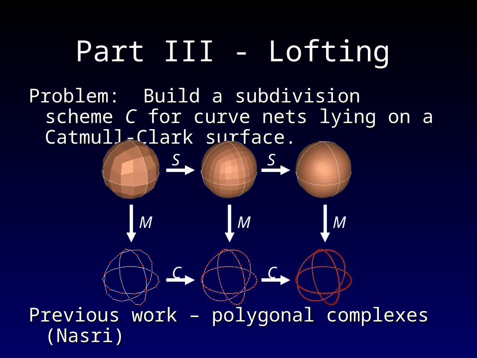
Part III - Lofting

Problem: Build a subdivision scheme Problem: Build a subdivision scheme CC for for curve nets lying on a Catmull-Clark surface.curve nets lying on a Catmull-Clark surface.

Previous work – polygonal complexes (Nasri)Previous work – polygonal complexes (Nasri)

S S

M M M

C C

A scheme for curve nets

Ordinary parts of Catmull-Clark surfaces are Ordinary parts of Catmull-Clark surfaces are bicubic splines. bicubic splines.

Subdivision rules for curve nets at:Subdivision rules for curve nets at: Valence two vertices – normal cubic rulesValence two vertices – normal cubic rules Valence four vertices – special interpolating Valence four vertices – special interpolating

rule for two intersecting cubicsrule for two intersecting cubics Other valences – next talkOther valences – next talk

An interpolating rule for cubics

Modify subdivision rules at vertex Modify subdivision rules at vertex vv of cubic of cubic such that such that vv always lies at its limit position always lies at its limit position

Cu Cu

C C

N N N

The commutative relation

Given subdivision matrix Given subdivision matrix CCuu for uniform for uniform

cubics and matrix cubics and matrix NN that positions that positions vv at limit, at limit, solve for non-uniform rules in solve for non-uniform rules in C C usingusing

C N = N CC N = N Cuu

10000

01000

061

32

610

00010

00001

N

81

43

8100

021

2100

081

43

810

0021

210

0081

43

81

uC

Solving for C using the relation

Solve for interpolating rules by inverting Solve for interpolating rules by inverting N.N. Yields special rules on two-ring of vertex Yields special rules on two-ring of vertex vv

Multiple cubics can interpolate Multiple cubics can interpolate vv

81

3223

163

3210

083

43

810

00100

081

43

830

0321

163

3223

81

1NCNCu

Understanding the new rules

Construct two or more polygons passing Construct two or more polygons passing through common vertex through common vertex vv

Apply rules to each polygon independentlyApply rules to each polygon independently

81

81

43

21

21




3223

321

81

163




83

81

43




1




Lofting the curve nets

Given curve scheme, find change of basis Given curve scheme, find change of basis MM where where CC commutes with commutes with SS for Catmull-Clark for Catmull-Clark

C M = M SC M = M S Observe that commutative relation impliesObserve that commutative relation implies

CCkk M = M S M = M Skk

Therefore, Therefore, SS∞∞pp00 interpolates interpolates CC∞∞qq00 where where

qq00=M p=M p00

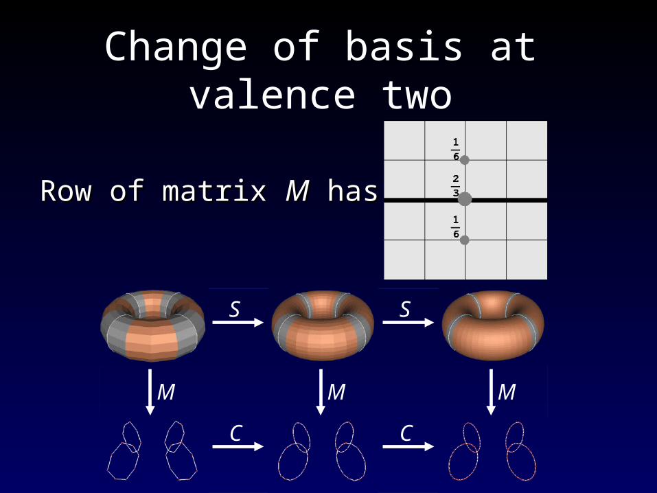
Change of basis at valence two

Row of matrix Row of matrix MM has form has form

S S

C C

M M M

Change of basis at valence four

Row of matrix Row of matrix M M has formhas form

S S

C C

M M M

Extraordinary vertices

For standard Catmull-Clark, curves passing For standard Catmull-Clark, curves passing through an extraordinary verts are through an extraordinary verts are notnot cubics cubics

Modify the subdivision rules in the Modify the subdivision rules in the neighborhood of extraordinary vertices to neighborhood of extraordinary vertices to allow interpolationallow interpolation

IdeaIdea: Fix curve net rules, generate modified : Fix curve net rules, generate modified surface rules at extraordinary verticessurface rules at extraordinary vertices

Generating modified surface rules

Expand commutative relation Expand commutative relation C M=M SC M=M S into into block formblock form

Solve locally for Solve locally for SS via block decomposition via block decomposition

Don’t form Don’t form SScc explicitly, use filters!explicitly, use filters!

n

cnc S

SMMMC

nncc SMCMMS 1

Conclusions

Many important types of analysis are possible Many important types of analysis are possible for subdivision schemesfor subdivision schemes

Linear algebra, especially commutative Linear algebra, especially commutative relations, is the key to these analysis methodsrelations, is the key to these analysis methods

Better theory supporting these analysis Better theory supporting these analysis methods is neededmethods is needed

Many thanks to Scott Schaefer!Many thanks to Scott Schaefer!

Documents

Analysis techniques for subdivision schemes Joe Warren Rice University