Analysis related to setting macroprudentialtools in the Czech Republic

(with emphasis on real estate related tools)Michal Hlaváček

Advisor to the Board Research DepartmentCzech National Bank

World Bank Macroprudential Workshop 2 June 2016

Disclaimer: The views and conclusions expressed in this presentation are solely those of the author and do not necessarily represent the official position of the Czech National Bank.

2

3

The macroprudential policy tools applied in the Czech Republic

• Recommendation on the management of risks associated with the provision of retail loans secured by residential property –16 June 2015

• The countercyclical capital buffer (set to 0.5% in Dec 2015)• The systemic risk buffer (buffer rates 1-3% fo 4 banks; 2014) • The capital conservation buffer (2.5% from 2014)

Seehttp://www.cnb.cz/en/financial_stability/macroprudential_policy/index.htmlfor details

I.Coping with housing exposures‘ risks

5

Real estate prices in the Czech Republic

• The apartment prices in the Czech Republic underwent also considerable recovery in 2015.

Transaction and asking prices of apartments in the CR(annual percentage changes)

Source: CNB Inflation Report, I/2016

-12

-9

-6

-3

0

3

6

9

12

I/11 I/12 I/13 I/14 I/15

Asking prices – PragueTransaction prices (tax returns) – PragueTransaction prices (survey) – PragueAsking prices – rest of CZTransaction prices (tax returns) – rest of CZTransaction prices (survey) – rest of CZ

6

• Faster growth in new loans for house purchase.• Interest rates on new loans for house purchase falling.

Conditions in housing market in 2013-2015

Year-on-year of housing credit growth(in %)

Source: CNB

2

4

6

8

01/12 07/12 01/13 07/13 01/14 07/14 01/15 07/15

New CZK housing loans interest rates (in %)

Source: CNB

2

3

4

1/12 7/12 1/13 7/13 1/14 7/14 1/15 7/15

7

Recommendation for credit institutions providing retail loans secured by residential property (I)

• The recommendation takes the form of a set of interconnected sub-recommendations (quantitative and qualitative) for banks, foreign bank branches and credit unions. • Credit institutions operating in the Czech Republic are mostly

prudent when providing loans secured by residential property. • However, there are signs of some easing of lending standards in

this segment. • The recommendation aims to prevent a loop between property

price growth and growth in loans posing a threat to the sector’s stability.• The individual recommendations define correct lending procedures

and standards. • They are aimed at enhancing existing internal risk management

systems in institutions and encouraging a prudent approach to lending.

8

• Recommendation A: • LTV < 100% & max 10% of new loans with LTV > 90% • Should not be circumvented through the concurrent provision of

unsecured consumer credit• Recommendation B:

• Institutions should set internal limits on indicators of clients’ ability to service loans from their own resources, e.g. limits on the LTI or DSTI ratio

• Recommendation C: • Max loan term 30Y & max term of unsecured consumer credit 8Y• Institutions should not provide loans secured by residential

property with a non-standard repayment schedule leading to a shift of the client’s credit commitments to a later period

Recommendation for credit institutions providing retail loans secured by residential property (II)

9

• Recommendation D:• Refinancing with increased principal – should be treated in the

same manner as in the case of new loans

• Recommendation E: • When working with loan intermediaries, institutions should apply a

prudent approach, considering the risks associated with the different interests of intermediaries and separately monitoring the quality of such loans

• Recommendation F:• For credit risk management purposes, institutions are

recommended to identify and separately monitor the different characteristics of owner-occupied and buy-to-let portfolios of loans

Recommendation for credit institutions providing retail loans secured by residential property (III)

10

• LTV limits were adopted in number of European countries• In some countries LTV limits are combined with LTI or DSTI limits • Other specific tools in/outside Europe:

• specific limits on buy-to-let loans, regional credit limits, higher sector-specific risk weights for the calculation of capital requirements etc.

LTV limits in Europe

Note: Data are simplified; possible exceptions / additional rules or stricter limit for specific loan categories may apply. DSTI limit based on net income. * From 2017.** From 2016.

0

1

2

3

4

0

15

30

45

60

75

90

105

NL DK* CZ FI** SK LV EE LT RO SE NO CY HU PO IELTV DSTI LTI (rhs)

II.Analysis related to setting the

recommendation- LTV/LTI Survey

12

Survey of credit standards for new loans secured by residential property (I)

• Sustained growth in property prices becomes a risk to financial stability if it is accompanied by an easing of lending standards.

• To assess the degree of easing of credit standards, the CNB conducted a survey among banks regarding the structure of new loans provided in 2014 according to two indicator categories:• LTV (loan-to-value) – the ratio of the loan amount to the value of collateral,• LTI (loan-to-income) – the ratio of the loan amount to the applicant's net income.• Joint distribution

• In 2015 similar survey (results not public yet) to asses how banks are fulfilling recommendation- survey based on micro data on individual loans, new information (price and valuation, DSTI, commercial real estate) • Additional types of analysis- stress tests on households, analysis of valuation

(x-axis: LTV in %; y-axis: share of loans in %)

Source: CNB

Comparison of the LTV distribution of new loans and the stock of loans

0

5

10

15

20

25

30

35

< 50 50–70 70–80 80-90 90–100 > 100

New loans Stock of loans

13

Assessment of credit standards for new loans secured by residential property (II)

• Loans with LTVs between 80% and 90% were the most frequent among the monitored categories of new loans.

• A skewed distribution is visible for new loans: average LTV 63%, median LTV 77%.

• The LTV distribution of new loans differs partly from the distribution of the stock of loans.

Distribution of new loans by LTV and bank size(x-axis: LTV in %; y-axis: share of loans in %)

Source: CNBNote: The breakdown by bank size does not necessarily correspond to the size of the market shares for loans for house purchase.

0

5

10

15

20

25

30

35

40

< 50 50–60 60–70 70–80 80–90 90–100 > 100

Total Small banks

Medium-sized banks Large banks

Building societies

14

• The survey results differ depending on institution size and type:

• a low share of loans with LTVs of over 90% for small and medium-sized banks,

• an increased share of new loans with high LTVs (over 90%) for large banks and building societies.

Assessment of credit standards for new loans secured by residential property (III)

Relationship between LTV and LTI for new loans(x-axis: LTV in %; y-axis: share of loans in %)

Source: CNB

0

10

20

30

40

50

60

70

< 70 70–80 80–100 > 100

LTI < 3 LTI 3–3.5 LTI 3.5–4 LTI 4–4.5 LTI 4.5–5 LTI 5–5.5 LTI > 5.5

15

• The LTI distribution of new loans is U-shaped. • Loans with very low (< 3) or very high (> 5.5) LTIs are the most

frequent.

Assessment of credit standards for new loans secured by residential property (III)

• There is a risky positive relationship between LTI and LTV. • Loans with high LTVs do

not always have low LTIs (are not drawn only by people with high income).

• By contrast, a rising LTI also means a rising share of loans with LTVs of 80%–100% and a higher average loan amount.

III.Analysis related to setting the

recommendation-A comprehensive method for house price sustainability

assessment, Hejlová, Hlaváček, CNB FSR 2014/15

What model of equilibrium house prices do we need?

• A perfect model of equilibrium house prices would have to capture:• meeting of demand and supply of housing• opportunity for investment into it, • limits to its affordability, • mutually reinforcing powers between house prices,

credit and real activity. • However, such structural model is far from being exercisable• Instead, we use more individual approaches which imitate

structure of such model and aggregate them

17

specific features of real estate

standard for any good

18

Assessment of equilibrium apartment prices

• The new formalised CNB approach combines four statistical and econometric models.

Determinants of SUPPLY

of housing

Financial sector

Real economy

Price of rents

HH income

Approach I:

Approach II:Accelerator

model

Approach III:Economic sense

of home ownership

Approach IV:Affordabilityof housing

Determinants of DEMAND

for housing

General supplyand demand

model

Approach I: Supply and demand model

• Approach• explaining equilibrium house prices using various supply and demand

determinants (firstly used by Hlaváček, Komárek, 2009)

• Estimation method• ordinary least squares

• Definition of house price gap• the part of house prices which cannot be explained by its determinants,

i.e. the OLS residuals including as many determinants as possible

• Comparison• inverted demand function estimated using simple OLS (similar to Kelly and

McQuinn, 2013)house price gap defined as the OLS residuals identifies “bubble from below” in 2013

19

Approach I: Supply and demand model

20

Graph 1 Graph 2Calibration of the model Estimated house price gap: (ths. CZK / m2) Comparison of Approach I to other models

(%)

Source: CNB calculations Source: CNB calculations

-10

-5

0

5

10

15

12/00 12/02 12/04 12/06 12/08 12/10 12/12 12/14

Supply and demand modelInverted demand model

-5

0

5

10

15

20

25

12/00 12/02 12/04 12/06 12/08 12/10 12/12 12/14

Tisíce

House pricesEquilibrium house pricesHouse price gap

Approach II: Financial accelerator model

21

• Approach• assessing the balance between house prices, credit on housing and real economic activity

• Estimation method• vector error correction model with Johansen cointegration

• Definition of house price gap• difference between actual house prices and their long run equilibrium value as estimated by

the Johansen cointegration

• Technical challenge• in steady state, is there some equilibrium house price trend to be included in the

cointegration? • capturing the upward trend of house prices after liberalization of the housing market in the

CR (this trend is hardly linear only)

• Comparison• existing approaches (ECB, 2011) define the house price gap as residuals from the VECM

this, however, tollerates the short run procyclicality of house prices

Approach II: Financial accelerator model

22

Graph 3 Graph 4Calibration of the model Estimated house price gap: (ths. CZK / m2) Comparison of different definitions of the gap

(%)

Source: CNB calculations Source: CNB calculations

-5

0

5

10

15

20

25

12/98 12/02 12/06 12/10 12/14

House pricesHouse price long run trendLong run equilibrium house pricesHouse price gap

-15

-10

-5

0

5

10

15

20

12/98 12/02 12/06 12/10 12/14

Long run (Johannsen cointegration gap)Long run and short run (VECM residuum)

Approach III: Adjusted ratio of house prices to rents

23

• Approach• assessing the ratio of prices to rents, adjusted for borrowing costs (LTV = 65%, M =

20Y) and tax deductibility of interest payments

• Assessment method• HP filter

• Definition of house price gap• percentage deviation of the ratio from the HP filter trend

• Technical challenge• in steady state, is the ratio stable? - increase in equilibrium house prices should pass through to

prices of rents, effect on ratio neutralized

• dealing with different speeds of liberalization of the market with housing and renting in the CR- assessing the ratio using HP filter vs. relative to the long run average

• Comparison • estimating the under or over valuation of house prices vs. that of annual costs of

housing as in Poterba (1984) or Himmelberg et al. (2005) the second approach disregards the character of housing as a storage of value problem of fixed vs. recurring costs of home ownership

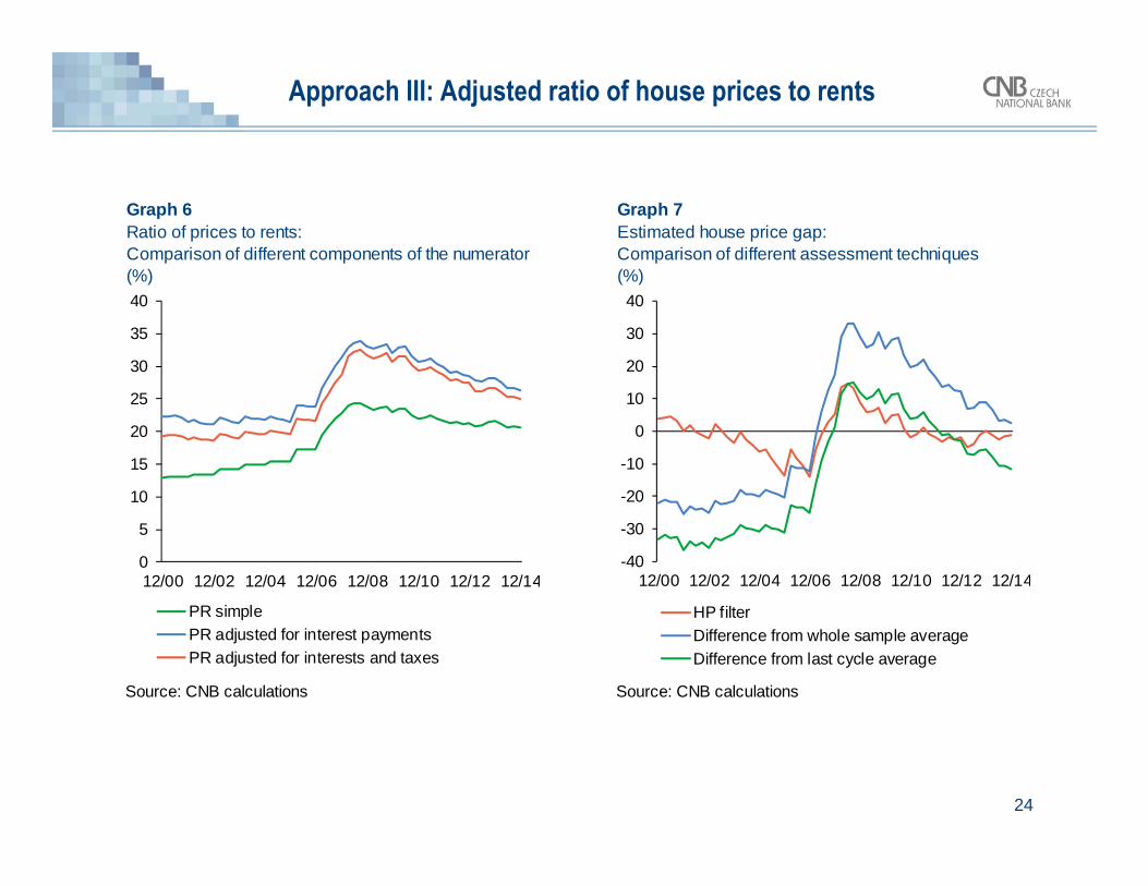
Approach III: Adjusted ratio of house prices to rents

24

Graph 6 Graph 7Ratio of prices to rents: Estimated house price gap: Comparison of different components of the numerator Comparison of different assessment techniques(%) (%)

Source: CNB calculations Source: CNB calculations

0

5

10

15

20

25

30

35

40

12/00 12/02 12/04 12/06 12/08 12/10 12/12 12/14

PR simplePR adjusted for interest paymentsPR adjusted for interests and taxes

-40

-30

-20

-10

0

10

20

30

40

12/00 12/02 12/04 12/06 12/08 12/10 12/12 12/14

HP filterDifference from whole sample averageDifference from last cycle average

Approach IV: Adjusted ratio of house prices to income

25

• Approach• assessing the ratio of prices to income, adjusted for borrowing costs (LTV = 65%, M

= 20Y) and tax deductibility of interest payments

• Assessment method• HP filter

• Definition of house price gap• percentage deviation of the ratio from the HP filter trend

• Technical challenge• in steady state, is the ratio stable?

suggestion for further analysis to be discussed at the end• dealing with upward trend of house prices after liberalization of the housing market in

the CR, when house prices might have been adjusting at different pace than wages assessing the ratio using HP filter vs. relative to the long run average

Approach IV: Adjusted ratio of house prices to income

26

Graph 8 Graph 9Ratio of prices to income: Estimated house price gap: Comparison of different components of numerator Comparison of different assessment techniques(%) (%)

Source: CNB calculations Source: CNB calculations

2

3

4

5

6

7

8

9

12/00 12/02 12/04 12/06 12/08 12/10 12/12 12/14

PTI simplePTI adjusted for interest payments (DSTI)PTI adjusted for interests and taxes

-20

-10

0

10

20

30

40

12/00 12/02 12/04 12/06 12/08 12/10 12/12 12/14

HP filterDifference from whole sample averageDifference from last cycle average

Results of individual approaches: Actual

• The individual approaches are• consonant in identifying periods of house

price under or overvaluation • somewhat different in estimating its size

• The expected differences between them more or less hold

27

Table 1Periods of house price under (green) and overvaluation (red): Comparison of results from approaches I-IV

Suppy and demand model #Financial accelerator model #Adjusted ratio of price to rent #Adjusted ratio of price to income #

2000 2001 2002 2003 2004 2011 2012 2013 20142005 2006 2007 2008 2009 2010

Graph 10Estimated house price gap: Comparison of results from approaches I-IV(%)(%)

Source: CNB calculations

-20

-15

-10

-5

0

5

10

15

20

25

12/00 12/02 12/04 12/06 12/08 12/10 12/12 12/14

Suppy and demand modelFinancial accelerator modelAdjusted ratio of prices to rentsAdjusted ratio of prices to income

• A weighted average indicates aslight overvaluation of apartment prices of 1.5%

• However, there is a strong regional dimension (prices in Prague and Brno are most overvalued)

• The risk of residential property prices becoming significantly overvalued is low for now

28

Results of individual approaches

Apartment price gap(%)

Source: CZSO, IRI, MRD, EC, CNB calculation

-10

-5

0

5

10

15

20

25

12/07 06/09 12/10 06/12 12/13 06/15

Supply and demand model

Adjusted price-to-income ratio

Adjusted price-to-rent ratio

Accelerator model

Table 1Periods of house price under (green) and overvaluation (red): Comparison of results from approaches I-IV

Suppy and demand model #Financial accelerator model #Adjusted ratio of price to rent #Adjusted ratio of price to income #

2000 2001 2002 2003 2004 2011 2012 2013 20142005 2006 2007 2008 2009 2010

Aggregation of results from individual approaches

• Weighting scheme based on premise that:• estimates „close“ to each other give strong

information about house price under or overvaluation of that size

• estimates „far“ from each other may each give additional information

• We arrived at two sets of weights:• they each give higher importance to

the estimates the more and less correlated they are, respectively

• The actual house price gap might lie in the interval given by these two sets of weights

29

Graph 11Estimated house price gap: Aggregation of approaches I-IV(%)

Source: CNB calculations

-15

-10

-5

0

5

10

15

12/00 12/02 12/04 12/06 12/08 12/10 12/12 12/14

Lower limit ("-")Upper limit ("+")Average + and -95% confidence intervalTable 2

Correlation coefficients between individual house price gap estimates and their weights

Approach I Approach II Approach III Approach IV + -Approach I 1.00 17.88% 36.69%Approach II 0.46 1.00 27.47% 20.94%Approach III 0.28 0.71 1.00 24.12% 26.44%Approach IV 0.59 0.88 0.80 1.00 30.52% 15.93%

Correlation coefficient Weight

Check for robustness of the aggregation method

• Some of the estimation and assessment methods may lead to results which are not consistent over time (“end point bias”) in such case, the most recent estimates

would be subject to higher uncertainty

• To check for this, we ran the whole houseprice assessment method on various samples of different length

• The method proved robust enough the highest bias realized on samples that

were too short

30

Graph 12Estimated house price gap: Comparison of aggregated estimates on samples(%)

Source: CNB calculations

-15

-10

-5

0

5

10

15

12/00 12/02 12/04 12/06 12/08 12/10 12/12 12/14

HP gap estimate on shorter samplesHP gap estimate on sample ending in 2014Q4

THANK YOU FOR YOUR ATTENTION

Contact:

Michal HlaváčekEconomic Research DepartmentCzech National BankNa Prikope 28CZ-11503 Prague

E-mail: michal.hlavacek@cnb.cz

Financial Stability Department in the CNB: financial.stability@cnb.cz

CNB: Financial Stability Reports, various issues -available at http://www.cnb.cz/en/financial_stability

32

References

HEJLOVÁ, H., HLAVÁČEK, M. (2015): A comprehensive method for house price sustainability assessment , Financial Stability Report 2014/2015 (pp. 121–130).

HLAVÁČEK, M., KOMÁREK, L. (2009): Housing Price Bubbles and their Determinants in the Czech Republic and its Regions. Czech National Bank Working Paper, 12/2009

ECB (2011). Tools for detecting a possible misalignment of residential property prices from fundamentals. Box 3 in ECB Financial Stability Review, June 2011, pp. 57-59.

HIMMELBERG, C., MAYER, C., & SINAI, T. (2005). Assessing high house prices: Bubbles, fundamentals, and misperceptions (No. w11643). National Bureau of Economic Research.

KELLY, R., & MCQUINN, K. (2013). On the hook for impaired bank lending: Do sovereign-bank inter-linkages affect the fiscal multiplier?. Central Bank of Ireland Research technical paper, 1.

POTERBA, J. M. (1984). Tax subsidies to owner-occupied housing: an asset-market approach. The quarterly journal of economics, 729-752.

PLAŠIL, M., J. SEIDLER, P. HLAVÁČ, T. KONEČNÝ (2014): An indicator of the financial cycle in the Czech economy, Financial Stability Report 2013/2014 (pp. 118–127).

Additional slides

Setting the Countercyclical capital buffer

(%)

Source: CNB

Assessment of the need to set a non-zero CCB rate in the Czech Republic

-2,5

-1,5

-0,5

0,5

1,5

2,5

-10

-6

-2

2

6

10

03/05 03/07 03/09 03/11 03/13 03/15Deviation of credit-to-GDP ratio from trendHypothetical CCB rate (rhs)

Results of application of BIS-ESRB* methodology

• Credit-to-GDP gap according to common reference guide based on:• total credit = all loans provided to the private sector + the volume of

bonds issued by the domestic private sector.• HP filter with λ of 400,000, time series: 1995 Q4 – latest.

34* Recommendation of the European Systemic Risk Board of 18 June 2014 on guidance for setting countercyclical buffer rates

Credit-to-GDP in the Czech Republic and its trend(estimated by HP filter, %)

Source: CNB

40

50

60

70

80

90

03/95 03/99 03/03 03/07 03/11 03/15Credit-to-GDPCredit-to-GDP trend (1995-)

Application of the methodology on a shorter time series

• shorter time series = not including transitional-crisis period,• time series: 2004 Q1 – latest.

35

(%)

Source: CNB

Assessment of the need to set a non-zero CCB rate in the Czech Republic

-1,5

-1

-0,5

0

0,5

1

1,5

-6

-4

-2

0

2

4

6

03/05 03/07 03/09 03/11 03/13 03/15Deviation of credit-to-GDP ratio from trendHypothetical CCB rate (rhs)

Credit-to-GDP in the Czech Republic and its trend(estimated by HP filter, %)

Source: CNB

40

50

60

70

80

90

03/95 03/99 03/03 03/07 03/11 03/15Credit-to-GDPCredit-to-GDP trend (1995-)Credit-to-GDP trend (2004-)

More comprehensive assessment applied

36

• Overall assessment published quarterly as a part of „Provision on setting the countercyclical capital buffer rate“.

• Credit-to-GDP gap(s).• FCI as a composite indicator.• Group of partial indicators such as

• bank credit growth,• speed of private sector borrowing relative to income,• bank lending standards,• debt service relative income,• residential property prices,• capital market dynamics.

Aggregate indicator of the financial cycle(0 minimum, 1 maximum, latest 09/2015)

Source: CNB

0,0

0,1

0,2

0,3

0,4

0,5

0,6

03/04 03/06 03/08 03/10 03/12 03/14

General lending standards in the Czech Republic(difference in market share of banks in pp)

Source: Bank lending survey, CNB

-60

-50

-40

-30

-20

-10

0

10

20

30

40

09/12 03/13 09/13 03/14 09/14 03/15 09/15

Housing loans Consumer and other loans

Sole proprietors Non-financial companies

37

Assessment of position in financial cycle

• The financial cycle in the Czech Republic is in a recovery phase: • The aggregate indicator of the financial cycle is rising gradually.

• An easing of banks’ credit standards indicates a shift to a more expansionary phase of the cycle.

38

Identification of stage in financial cycle

• For detecting the stage in financial cycle and capturing systemic risk build-up we developed the Financial Cycle Indicator (FCI; Plašil et al., 2014).

The FCI and its decomposition(0 minimum, 1 maximum)

Source: Authors’ calculations using CNB and CZSO data

-0,6

-0,4

-0,2

0,0

0,2

0,4

0,6

0,8

1,0

09/04 12/06 03/09 06/11 09/13 12/15Credit - households Credit - NFCsProperty prices Debt/disp.incomeDebt/op.surplus Credit cond. - householdsCredit cond. - NFCs PX50CA deficit/GDP Contrib. of corr.FCI