Embed Size (px)
Citation preview

ORIGINAL RESEARCH PAPERS
Analysis of Wheel-Roller Contact and Comparisonwith the Wheel-Rail Case
Binbin Liu1 • Stefano Bruni1
Received: 13 November 2015 / Revised: 14 December 2015 / Accepted: 19 December 2015 / Published online: 12 January 2016
� The Author(s) 2016. This article is published with open access at Springerlink.com
Abstract Full-scale roller rigs are recognized as useful
test stands to investigate wheel-rail contact/damage issues
and for developing new solutions to extend the life and
improve the behaviour of railway systems. The replace-
ment of the real track by a pair of rollers on the roller rig
causes, however, inherent differences between wheel-rail
and wheel-roller contact. In order to ensure efficient uti-
lization of the roller rigs and correct interpretation of the
test results with respect to the field wheel-rail scenarios, the
differences and the corresponding causes must be under-
stood a priori. The aim of this paper is to derive the dif-
ferences between these two contact cases from a
mathematical point of view and to find the influence factors
of the differences with the final aim of better translating the
results of tests performed on a roller rig to the field case.
Keywords Wheel-rail contact � Wheel-roller contact �Creepage � Contact patch � Roller rig
1 Introduction
The contact between wheel and rail is one of the most
important features of the railway system, and this contact
pair has attracted great attention since the beginning of
railway engineering. Unfortunately, the problems involved
in the wheel-rail contact interface have not been
completely solved due to the complexity of the problem.
Many attempts have been made from both theoretical and
experimental points of view. Moreover, field experiments
on wheel-rail contact mechanics and dynamics are often
challenging due to the difficulties in adequately controlling
the test conditions [1]. Roller rigs are a good alternative in
this case, thanks to their high controllability and flexibility,
and have been used as experimental tools in railway
application over a long time. A variety of roller rig designs
have been introduced, targeting different research aims,
more detail on this topic can be found in [2–4].
A. Jaschinski et al. [2] performed a comprehensive survey
for both full-scale and scaled model roller rigs on the
application to railway vehicle dynamics. Zhang et al. [4]
reviewed the development history of the roller rig for
railway application and performed a detailed comparison
between rollers and track in terms of geometry relationship
with wheel, creep coefficient, stability, vibration response
and curve simulation. Allen [5] and Yan [6] documented in
detail on the errors caused by scaled roller rigs for the study
of the dynamic behaviour of railway bogies. Keylin et al.
[1] derived explicit analytical expressions for comparing
contact patch dimensions and Kalker’s coefficients for a
wheel moving on a roller and on a tangent track, based on
Hertz and Kalker’s linear theory. Taheri et al. [7] compared
the contact patch formed by a single wheelset when cou-
pled to a roller and to a tangent track under the assumptions
of the Hertz’s theory. Zeng [8] compared the geometry
contact characteristics of the wheel-rail and that of the
wheel-roller based on a three-dimensional contact search-
ing method.
Nevertheless, a systematic analysis of wheel-roller
contact and the differences with respect to the wheel-rail
case are missing in the literature. It should be noted that the
roller rig test will never completely replace the field test
& Binbin Liu
1 Dipartimento di Meccanica, Politecnico di Milano, Via La
Masa 1, 20156 Milan, Italy
Editor: Xuesong Zhou
123
Urban Rail Transit (2015) 1(4):215–226
DOI 10.1007/s40864-015-0028-3 http://www.urt.cn/

due to inherent differences caused by the replacement of
the rail by rollers in a roller rig system. Therefore, it is very
important to know the differences between these two sys-
tems and the corresponding reasons in order to efficiently
perform wheel-rail contact study on a roller rig and to
correctly interpret the test results and to compensate for
deviations between the roller rig and a real track. This
analysis should cover in particular
– the geometry of wheel-rail/wheel-roller contact;
– differences in the formation of the contact patch;
– factors affecting the creepages in a test performed on a
roller and their effect on tangential contact forces.
The aim of this paper is to provide a thorough exami-
nation of the differences between these two contact cases
from a mathematical point of view and to find the influence
factors of the differences for better translating the test
results on the roller rig to the field test. To this aim, a new
approach for solving the normal contact problem for the
wheel-roller couple is proposed, and the expressions of the
creepages and spin are obtained for the wheel-roller couple.
The results of this new approach are presented comparing
the case of the wheelset running on a standard track and on
rollers, and the differences between these two cases are
discussed in the light of their effects on surface damage and
degradation occurring in the wheels and the rails.
2 Full-Scale Roller Rigs for Tests on a SingleWheelset
Among all of the roller rigs existing in laboratory, the full-
scale roller rig for a single wheelset test is one of most
similar systems to a real wheelset-track system from both
dynamics and contact mechanics points of view. The
mechanical layout for a roller rig of this type is shown in
Fig. 1. It consists of a roller with two wheels driven by a
motor. A full-scale wheelset is mounted on the top of two
rollers with real rail profiles and connected through pri-
mary suspensions to a transversal beam representing one
half of the bogie frame. Compared with the roller rig for
test on a complete vehicle, the high controllability and
flexibility of the single wheelset roller rig make it possible
to obtain adequate data on the dynamics of the system and
on wheel-rail contact under various conditions which are
essential for investigating the adhesion and creep of the
wheel over the rail. This configuration of the roller rig
allows to perform studies of wheel-rail interaction and also
tests concerning the dynamic behaviour of a wheelset/bo-
gie, see [9, 10]. However, this paper only concentrates on
wheel-rail contact.
3 Contact Formulation for Wheel-Rail and Wheel-Roller Systems
From a mathematical point of view, the contact problem
can be solved for both wheel-rail and wheel-roller contact
according to the following four steps [11, 12]. The first
step is to solve the geometrical problem, in which the
locations of the contact points on the contacting bodies are
determined. This is followed by solving the normal con-
tact problem, in which the shape and size of the contact
patch formed in the contact interface due to body defor-
mation and the corresponding pressure distribution over
the contact patch are determined. The third step is to deal
with the kinematic problem, in which normalized kine-
matic quantities, the so-called creepages, are determined.
These quantities measure the relative velocities between
the contacting bodies at the contact points. In the final
step, the tangential problem is solved; this concerns the
prediction of tangential stresses at the contact interface
which is generated by friction and creepages within the
contact zone [11, 13, 14]. All these steps need to be dealt
with differently for the case of wheel-roller contact
compared to the wheel-rail case, as described in the next
section.
3.1 Geometrical Problem
The contact geometry analysis deals with the contact point
searching problem between the contacting bodies, i.e.
wheel-rail and wheel-roller pairs in this case. The location
of contact depends on the dynamic conditions as well as
material properties of the contact pair if body deformation
is considered. There are many approaches for the detection
of the contact points for wheel-rail contact as documented
in [11]. Most of the approaches available in the literature
assume that the yaw angle of the wheelset against the track
is very small and negligible when solving the geometricFig. 1 Layout of a full-scale roller rig for a single wheelset test
216 Urban Rail Transit (2015) 1(4):215–226
123

contact problem so as to form the so-called bi-dimensional
methods [14]. This assumption largely simplifies the cal-
culation, leading to fast solutions that can be implemented
in rail vehicle online dynamics simulation. However, the
replacement of the rail by a roller makes the geometric
contact problem more complicated, and the traditional bi-
dimensional methods may not be applicable any longer due
to the considerable yaw influence on the contact location in
the case of the wheel-roller contact. To deal with this
problem, a three-dimensional model is needed. Some
existing approaches for wheel-roller geometry contact
analysis can be found in [4, 8, 15].
It is clear that the geometric contact condition between
the wheel and rail/roller is the same for zero yaw angle
conditions assuming the contacting bodies to be rigid. The
comparisons on the geometry contact relationship between
the wheel-rail and wheel-roller contact pairs are available
in the literature, for instance [4, 8, 12]. Therefore, no fur-
ther discussion is needed here, but one typical case study is
shown in Fig. 2 for the completeness of this study. The
calculation conditions are as follows: profile combination
is new S1002/UIC60 with 1:20 rail inclination, the radius
of the roller is 1 m and the yaw angle of the wheelset is
60 mrad.
It is interesting to note in Fig. 2 that two-point contact
occurs when the wheelset is shifted by 5 mm approxi-
mately in lateral direction for wheel-rail contact, but this
value is slightly different on the roller rig due to the
curvature of the rollers. Obviously, the differences can be
decreased by increasing the radius of the roller, but the
dimension of the roller is limited in practice considering
the increased cost and difficulties related with the man-
ufacturing and installation of the rig. It should be also
noted that 60 mrad is a quite large yaw angle for the
wheelset and that smaller differences are found for
smaller yaw angles.
3.2 Normal Problem
The well-known Hertzian theory [16] is widely used for
solving the normal contact problem in rail vehicle
dynamics simulation for its simplicity and calculation
efficiency. However, Hertzian theory is valid based on
half-space assumption and elliptic contact condition. In
order to obtain more realistic contact information for the
purpose of comparison between wheel-rail and wheel-roller
contact (especially in terms of shape and size of the contact
patch and of pressure distribution), the use of a more
advanced contact model is required. The most elaborate
contact model to date can be established by finite element
method [17, 18] which is quite complicated and time
consuming. The same problem can be dealt with using the
boundary element method as done, e.g. by Prof. Kalker’s
algorithm CONTACT [19] and by the model proposed by
Knothe and Le The in [20]. The so-called approximate
contact methods represent a trade-off between efficiency
and accuracy in the solution of the normal problem and
therefore are generally considered as best suited for both
local contact analysis and for online dynamics simulation.
Well-known approximate models include the Kik–Pio-
trowski model based on virtual penetration concept [21–
23], the STRIPES model proposed by Ayasse and Chollet
[24] and Linder’s model [25]. Some interesting surveys of
the existing approximate methods and the comparison and
analysis among them can be found in [22, 26].
The Kik–Piotrowski model has been chosen as the basis
for this study. Some modifications have been introduced to
extend the original method to deal with both wheel-rail and
wheel-roller contact conditions. The Kik–Piotrowski model
is a fast and non-iterative method to calculate normal
contact problem. An outline of this method will be given in
this section, for more details the reader is referred to [21–
23]. The idea of this method is presented in Fig. 3. When
(a) (b)
Fig. 2 Comparisons of the contact location on wheel in lateral (a) and longitudinal (b) directions with 60 mrad yaw angle
Urban Rail Transit (2015) 1(4):215–226 217
123

the undeformed surfaces of wheel and rail/roller, touching
in the geometrical point of contact O which is determined
from geometric contact analysis, are shifted towards each
other by a distance d, called the penetration, they penetrate
and intersect on a closed line, whose projection on the
x-y plane is called the interpenetration region. On the basis
of some similarity of shapes of the contact zone and
interpenetration region, the contact zone is determined by
scaling the interpenetration depth do = ed with an
approach scaling factor of e = 0.55 and the resulting
interpenetration region is taken as the real contact zone.
In order to solve the problem numerically, a coordinate
system Oxyz representing the contact reference system is
defined firstly with the x-axis pointing along the rolling
direction of the wheelset, and the y-axis parallel to the
wheel axle. The undeformed surface with the same x, y
coordinates in contact reference system is assumed as
zðx; yÞ ¼ fyzðyÞ þ1
Rw
þ 1
Rr
� �x2
2; ð1Þ
where subscript yz stands for the function defined in y-z
plane and Rw and Rr are the principal radii of the wheel and
rail/roller, respectively, at the geometrical point of contact
in rolling direction. For wheel tread and rail top contact Rr
goes to infinite, while this is not the case for the wheel-
roller contact case. The separation of profiles fyz(y) =
zyzw(y) ? zyz
r (y) is obtained from the sum of the cross-sec-
tions zyzw(y) of the wheel rolling surface and zyz
r (y) of the rail
surface by x = 0 in the contact plane. To proceed with the
presentation of the method, the interpenetration function of
the profiles is defined in the contact plane as
gyzðyÞ ¼d0 � fyzðyÞ if fyzðyÞ� d00 if fyzðyÞ[ d0
�ð2Þ
where d0 is the virtual interpenetration. The width of the
contact patch can be determined by solving Eq. (2). It
should be mentioned that the contact shape can be cor-
rected by adjusting the interpenetration function, cf. [22,
23], but no shape correction is applied in this study for
simplicity.
The contact zone is determined by the x coordinates of
its leading and trailing edges described by formula (3) in
the original method based on the assumption that the
wheel-rail contact problem is stated in terms of two bodies
of revolution with their axes laying in the same plane. The
same assumption was made by Linder [25].
xlxzðyÞ ¼ �xtxzðyÞ �ffiffiffiffiffiffiffiffiffiffiffiffiffiffiffiffiffiffiffiffi2RwgyzðyÞ
qð3Þ
where subscript xz means that the function is defined in the
x-z plane and superscripts l and t indicate the terms asso-
ciated with the leading and trailing edges of the contact
patch, respectively.
In order to determine the contact boundary for wheel-
roller contact, the following modifications of Eq. (3) are
proposed. Firstly, the contact patch is partitioned into strips
paralleling with the x-axis towards to the rolling direction
of the wheel. Hence, the profile functions are converted to
discrete forms by strips yi (i = 1…n). Then, the extremities
of each strip can be determined by solving Eq. (4) instead
of Eq. (3). The two solutions of Eq. (4) for each strip
correspond to the coordinates of the leading and trailing
edges of that strip. All the coordinates comprise the
boundary of the contact zone.
zwxzðx; yiÞ � zrxzðx; yiÞ ¼ gyzðyiÞ ð4Þ
where gyz (yi) is the interpenetration function at the i-th
strip in contact patch, zxzw(x,yi) and zxz
r (x,yi) are the rolling
circle of the wheel and roller with the radius of Rcw(yi) and
Scr(yi), respectively, over the i-th strip, which are expressed
by Eqs. (5) and (6).
zwxzðx; yiÞ ¼ RcwðyiÞ �ffiffiffiffiffiffiffiffiffiffiffiffiffiffiffiffiffiffiffiffiffiffiffiffiffiR2cwðyiÞ � x2
qð5Þ
zrxzðx; yiÞ ¼ ScrðyiÞ �ffiffiffiffiffiffiffiffiffiffiffiffiffiffiffiffiffiffiffiffiffiffiffiS2crðyiÞ � x2
qð6Þ
where x [ [-Rcw(yi), Rcw(yi)] is the longitudinal coordinate
of the rolling circle in the contact plane. It should be noted
that Scr(yi) is a straight line in the case of tangent track.
Moreover, it is assumed that the normal pressure is
semi-elliptical in the direction of rolling and has the fol-
lowing expression:
pðxj; yiÞ ¼p0
xlð0Þ
ffiffiffiffiffiffiffiffiffiffiffiffiffiffiffiffiffiffiffiffiffiffiffiffiffiffiffiffiffiffiffiffiffiffixlxzðyiÞ� �2�x2
jðyiÞ
q: ð7Þ
Fig. 3 Contact zone determined with virtual interpenetration method,
adapted from [21]
218 Urban Rail Transit (2015) 1(4):215–226
123

Following the same procedure documented in Ref. [21],
the normal contact problem can be solved numerically for
both wheel-rail and wheel-roller contact system.
It should be pointed out that the influence of the
wheelset’s yaw angle on the normal contact solution is
essential for wheel-roller contact and can be included based
on the similar idea proposed here, but it will not be dis-
cussed further in the current paper for simplicity.
3.3 Kinematical Problem
With reference to Fig. 1, it can be seen that the wheelset on
the roller rig has the same degrees of freedom as on a track,
except the constraint in longitudinal direction. Further-
more, the two rollers fixed on the same axle can only rotate
around its axle. To accomplish the kinematic analysis of a
wheelset on a pair of rollers, a convenient set of reference
frames should be introduced as shown in Fig. 4. The
wheelset reference frame is denoted by OwXwYwZwattached to the wheelset’s centre of mass so that axis OwYwcoincides with the wheelset’s axis of rotation, the OwZwaxis points upwards and the OwXw axis completes the right-
handed coordinate system. Similarly, a roller reference
frame is introduced and denoted by OroXroYroZro attached
to the roller’s centre of mass which is defined as the inertial
frame. Two contact reference frames OclXclYclZcl and
OcrXcrYcrZcr are introduced at the contact interfaces
between the left-hand and right-hand wheels of the
wheelset and rollers at the wheelset central position.
It is assumed that the wheelset reference frame
OwXwYwZw is obtained from the inertial frame by per-
forming two successive rotations. The axes of the refer-
ence frames are parallel before rotation, and the first
rotation is made about the z-axis by an angle w called
yaw angle (positive in counter-clockwise direction) fol-
lowed by a second rotation about the x-axis by an angle ucalled roll angle. Therefore, the transformation matrix
Aw2i connecting the wheelset frame to the inertial frame is
expressed as follows:
Aw2i ¼cosw � sinw 0
sinw cosu cosw cosu � sinusinw sinu cosw sinu cosu
24
35 ð8Þ
Since the angles of rotation are generally small in rail-
way dynamics, the small angle approximation can be
applied, so that the transformation matrix reduces to
Fig. 4 Reference frames defined in the roller rig system
Urban Rail Transit (2015) 1(4):215–226 219
123

Aw2i �1 �w 0
w 1 �u0 u 1
24
35: ð9Þ
The position vectors of the contact points on the wheel and
roller can be defined in the inertial frame as follows:
rwi ¼ Rw þ Aw2i�uwi ði ¼ l; rÞ ð10Þ
where the position vector of the origin of the wheelset
reference frame in the inertial frame is expressed as
Rw ¼ 0 y z½ �T ð11Þ
and the position vectors of the contact points in the
wheelset reference frame can be expressed in the following
forms: for the left-hand wheel
�uwl ¼ ½rlsinb l � rlcosb�T ð12Þ
and for the right-hand wheel
�uwr ¼ ½�rrsinb �l �rrcosb�T; ð13Þ
where ri (i = l,r) represents the radius of the left-hand and
right-hand wheels, respectively, l is the half distance
between the contact points on the left-hand and right-hand
wheels and b is the shift angle of the contact point on the
roller with respect to the vertical plane of the inertial frame
caused by a non-zero yaw angle w. It is assumed that this
angle is the same for the left-hand and right-hand side on
the roller and can be approximated by Eq. (14), since it is
very small in ordinary circumstances.
b ¼ lwr0 þ s0
ð14Þ
In Eq. (14), r0 and s0 denote the radii of the wheel and
roller at the central position, respectively.
Taking the derivative of Eq. (11), the velocity vector of
the contact point located on the wheel with respect to the
inertial frame is obtained as
vwi ¼ _Rw þ xw � uwi ði ¼ l; rÞ; ð15Þ
where uwi ¼ Aw2i�uwi is the position vector of the point of
contact on the wheel defined in the inertial frame which is
determined from Eqs. (9), (12) and (13) for the left-hand
and right-hand wheels, respectively, as follows:
uwl ¼ Aw2i�uwl �rl sin b� lw
rlw sin bþ lþ rlu cos blu� rl cos b
24
35
�rlb� lwlþ rlulu� rl
24
35 ð16Þ
and
uwr ¼ Aw2i�uwr ��rr sin bþ lw
�rrw sin b� lþ rru cos b�lu� rr cos b
24
35
��rrbþ lw�lþ rru�lu� rr
24
35 ð17Þ
and xw is the absolute angular velocity vector at the point
of contact defined in the inertial system as
xw ¼0
0_w
24
35þ Aw2i
_uXw
0
24
35 ¼
_u cosw� Xw sinw cosu_u sinwþ Xw cosw cosu
_wþ Xw sinu
24
35
�_u� Xww_uwþ Xw_wþ Xwu
24
35
ð18Þ
with Xw = V/r0 the rolling angular velocity of the
wheelset.
Substituting Eqs. (11), (17) and (18) into Eq. (15), the
velocity vectors of the contact point on the wheelset in the
inertial frame are obtained as follows. For the left-hand
wheel:
vwl ¼ _Rw þ xw � uwl
��l _w� rlð _uwþ _wuþ XwÞ
_y� lð _uuþ _wwÞ þ rlð _uþ _wb� XwwÞ_zþ l _uþ rlð _uu� XwbÞ
24
35 ð19Þ
and for the right-hand wheel:
vwr ¼ _Rw þ xw � uwr
�l _w� rrð _uwþ _wuþ XwÞ
_yþ lð _uuþ _wwÞ þ rrð _u� _wb� XwwÞ_z� l _uþ rrð _uuþ XwbÞ
24
35: ð20Þ
Similarly, the velocity vector of the contact point on the
roller in the inertial frame can be expressed as
vroi ¼ xro � uroi ði ¼ l; rÞ; ð21Þ
where xro is the angular velocity of the roller with the
following form:
xro ¼0
Xor
0
24
35 ¼
0
� V
s00
264
375 ð22Þ
and uroi stands for the position vector of the contact point in
the inertial frame. For the left-hand roller, the expression of
this vector is
urol ¼ ½�slsinb l slcosb�T ð23Þ
and for the right-hand roller the expression is
220 Urban Rail Transit (2015) 1(4):215–226
123

uror ¼ ½srsinb �l srcosb�T: ð24Þ
Hence, the velocity vector of the point of contact is
obtained. For the left-hand roller,
vrol ¼ xro � urol ¼0
� V
s00
264
375�
�sl sinbl
sl cos b
24
35
¼� V
s0sl cos b
0
� V
s0sl sin b
26664
37775 �
� V
s0sl
0
� V
s0slb
26664
37775 ð25Þ
and for the right-hand roller:
vror ¼ xro � uror ¼0
� V
s00
264
375�
sr sin b�l
sr cos b
24
35
¼� V
s0sr cos b
0V
s0sr sin b
26664
37775 �
� V
s0sr
0V
s0srb
26664
37775: ð26Þ
Thus, the velocity differences between the wheel and
roller at each point of contact in the inertial frame can be
calculated as follows. For the left side
Dvl ¼ vwl � vrol
¼�l _w� rlð _uwþ _wuþ XwÞ þ
V
s0sl
_y� lð _uuþ _wwÞ þ rlð _uþ _wb� XwwÞ_zþ l _uþ rlð _uu� XwbÞ þ
V
s0slb
266664
377775 ð27Þ
for the right side:
Dvr ¼ vwr � vror
¼l _w� rrð _uwþ _wuþ XwÞ þ
V
s0sr
_yþ lð _uuþ _wwÞ þ rrð _u� _wb� XwwÞ_z� l _uþ rrð _uuþ XwbÞ �
V
s0srb
266664
377775 ð28Þ
and the difference of angular velocity is
Dx ¼ xw � xro ¼_u cosw� Xw sinw cosu
_u sinwþ Xw cosw cosuþ V
s0_wþ Xw sinu
264
375
�_u� Xww
_uwþ Xw þ V
s0_wþ Xwu
264
375:
ð29Þ
To determine the creepages and spin, the velocity dif-
ferences obtained above must be resolved in the contact
plane where they are defined. It is assumed that the contact
frames are connected to the wheelset frame by the fol-
lowing transformation matrices for the left and right
wheels, respectively.
Aw2cl ¼cos b 0 sinb
� sin b sin dl cos dl cos b sin dl
� sin b cos dl � sin dl cos b cos dl
24
35
�1 0 b0 1 dl�b �dl 1
24
35 ð30Þ
and
Aw2cr ¼cos b 0 � sin b
� sinb sin dr cos dr � cos b sin drsin b cos dr sin dr cos b cos dr
24
35
�1 0 �b0 1 �drb dr 1
24
35; ð31Þ
where di(i = l,r) denotes the contact angle.
Hence, the transformation matrices connecting the
inertial frame to the contact frame can be obtained for the
left and right side wheels by the following operation. For
the left side
Ai2cl ¼ Aw2clAi2w ¼ Aw2clðAi2wÞT
�1 w b�w 1 dl þ u�b �dl � u 1
24
35 ð32Þ
and for the right side:
Ai2cr ¼ Aw2crAi2w ¼ Aw2crðAi2wÞT
�1 w �b�w 1 �dr þ ub dr � u 1
24
35 ð33Þ
Therefore, the velocity differences between the wheel
and roller in the contact plane are obtained as
Dvci ¼ Ai2ciDvi
Dxci ¼ Ai2ciDxi
: ð34Þ
Now, the creepages can be obtained by definition as
follows. The longitudinal creepages on the left and right
wheels are
nlx ¼DvclxV
� � l _wV
� rl _wuV
� rl
r0þ _yw
Vþ sl
s0þ _zb
Vþ l _ub
V
nrx ¼DvcrxV
� l _wV
� rr _wuV
� rr
r0þ _yw
Vþ sr
s0� _zb
Vþ l _ub
V
ð35Þ
Urban Rail Transit (2015) 1(4):215–226 221
123

the lateral creepages are
nly ¼DvclyV
�_y� sl
s0wV þ rl _wbþ rl _uþ ldl _uþ _zdl þ _zu
V
nry ¼DvcryV
�_y� sr
s0wV � rr _wbþ rr _uþ ldr _uþ _zdr � _zu
V
ð36Þ
and the spin creepages are
nlz ¼Dxclz
V� � dl
r0þ
_wV� _ub
Vþ Xordl
Vþ Xoru
V
nrz ¼Dxcrz
V� dr
r0þ
_wVþ _ub
V� Xordr
Vþ Xoru
V
: ð37Þ
It can be seen from the expressions above that the radius
of the roller and the shift angle (function of yaw) contribute
to the differences in terms of creepages and spin with
respect to wheel-rail contact condition. The corresponding
expressions for wheel-rail contact condition can be
obtained by setting s0 = ? and b = 0. Moreover, the
longitudinal and lateral creepages can be simplified further
by assuming that the contacting bodies remain in contact at
all times which means the z components vanish in the
expressions (35) and (36).
3.4 Tangential Problem
The common method to solve the wheel-rail tangential
contact problem is represented by the FASTSIM algorithm
[13], also due to Kalker. This method was originally
developed for elliptic contact condition, but can be exten-
ded to cover a more general geometry of the contact patch.
The difficulty is to determine the flexibility parameter that
is required by this method. To overcome this, Kik and
Piotrowski proposed a method to define an equivalent
ellipse for each separate contact zone by setting the ellipse
area equal to the non-elliptic contact area and the ellipse
semi-axes ratio equal to length to width ratio of the patch.
The flexibility parameter is determined by equating the two
solutions obtained from the linear complete theory and
from the simplified theory for elliptical contact area and
pure longitudinal, lateral and spin creepages. In addition,
there are two options with respect to the choice of the
flexibility parameter, namely considering one single
weighted mean flexibility parameter or three flexibility
parameters one for each creepage component. According to
[27], the single flexibility parameter will reduce the
agreement of FASTSIM to the exact theory. Therefore,
three flexibility parameters are used in the current study.
From the main assumption of the linear theory which
neglects slip in the contact zone, the tangential stress dis-
tribution is derived in the form:
sxðx; yÞ ¼nxL1
� ynzL3
ðx� xlxzÞ
syðx; yÞ ¼nyL2
ðx� xlxzÞ þnz2L3
x2 � xlxz� �2�
8>><>>:
ð38Þ
where ni(i = 1 - 3) are the longitudinal, lateral and spin
creepages, and Li(i = 1 - 3) denotes the flexibility
parameter for each creepage component.
The stresses stated in Eq. (38) cannot exceed the so-
called traction bound. Slip occurs in the region where the
tangential stresses predicted by Eq. (38) are greater than
the traction bound. The formulation for the traction bound
used in this paper is obtained by applying Coulomb’s
friction law locally with a constant friction coefficient, i.e.
lp(xi,yj). The tangential forces are obtained from the
numerical integration of the stresses over the contact patch.
4 Results and Discussions
The effects of roller rig testing in the experimental inves-
tigation of wheel-rail contact have been addressed in
Sect. 3 under four different points of view. In reality, all of
these factors interact with one another, thereby it is
essential to investigate their combined influence on the
contact solution. To this end, a set of cases with various
contact positions and radii of roller have been chosen to
quantify the influence. The calculation parameters listed in
Table 1 are used throughout the simulations.
For simplicity, the track irregularities are neglected and
no wheelset velocity component is considered except in the
rolling direction. The creepages are calculated according to
expressions (35)–(37) as presented in Table 2. According
to Eq. (35), the last three terms represent the additional
Table 1 Calculation parameters
Parameter type Value
Wheel profile New S1002
Rail/roller profile New UIC60
Rail/roller inclination 1:40
Track/roller gauge 1435 mm
Wheel flange back spacing 1360 mm
Tape circle to flange back distance 70 mm
Wheel radius 460 mm
Roller radius 0.5 m/1.0 m
Young’s modulus 210 MPa
Poisson’s ratio 0.3
Friction coefficient 0.35
Normal force 80 kN
Velocity 72 km/h
222 Urban Rail Transit (2015) 1(4):215–226
123

contribution of the roller rig to the longitudinal creepage
with respect to wheel-rail contact case. It is clear that the
major difference in the longitudinal creepage is caused by
the variation of the roller head circumferential velocity
across its profile. The lateral creepage is zero when the yaw
angle is assumed to be zero based on Eq. (36) under the
considered contact condition. It can be seen from Eq. (37)
that the additional contribution of the roller rig to the spin
creepage is coming from the last three terms in the
expression that represents, respectively, the effect of the
wheelset yaw angle and of the angular velocity of the
roller. These additional terms explain the remarkable
increase of the spin for the roller rig case which is shown in
Table 2. The contact estimation results are presented in
two groups for normal contact solution and tangential
contact solution, respectively.
4.1 Normal Contact Solution
The solutions of the normal contact problem in terms of the
shape and area of the contact patch and the corresponding
pressure distribution within the contact region are obtained
by the method proposed in Sect. 3.2 for wheel-rail and
wheel-roller contact conditions, respectively. The calcula-
tion results for the case studies listed in Table 2 are pre-
sented in Fig. 5, and the results of wheel-rail contact and of
wheel-roller contact obtained at the same contact position
are presented in the same figure for comparison.
It can be seen from Fig. 5 that these two simulation
cases correspond to a highly non-elliptic contact condition
in the first case and nearly elliptic contact condition in the
second case. In Fig. 5a, b, it is observed that the length of
the contact patch in longitudinal direction decreases for the
roller rig with respect to the rail due to the finite radius of
roller, this effect being more visible for the smaller value of
the roller radius. On the contrary, the width of the contact
patch is slightly increased in the case of wheel-roller
contact. The maximum contact pressure over the contact
zone is increased by a decrease of the roller radius as the
same load is spread across a smaller contact area, see
Fig. 5c, d. The change of the contact patch also affects the
semi-axis ratio and consequently affects the creep coeffi-
cient and the creep forces. The differences caused by the
roller rig in terms of contact area and maximum contact
pressure should be taken into account when the roller rig is
used for contact deterioration mechanism studies such as
wear and rolling contact fatigue. To quantify the difference
involved in the normal contact solution, a statistical sum-
mary of the results is presented in Table 3.
It can be concluded from Table 3 that the differences are
increasing with the decrease of radius of the roller and the
agreement between wheel-roller and wheel-rail contact is
better for the approximately elliptic contact condition, i.e.
case 2. It should be mentioned that the results reported here
are dependent on the particular parameters assumed in this
study, but the analysis approach and the conclusions are
generally applicable to any roller rig of this kind.
4.2 Tangential Contact Solution
The corresponding tangential contact solutions for the
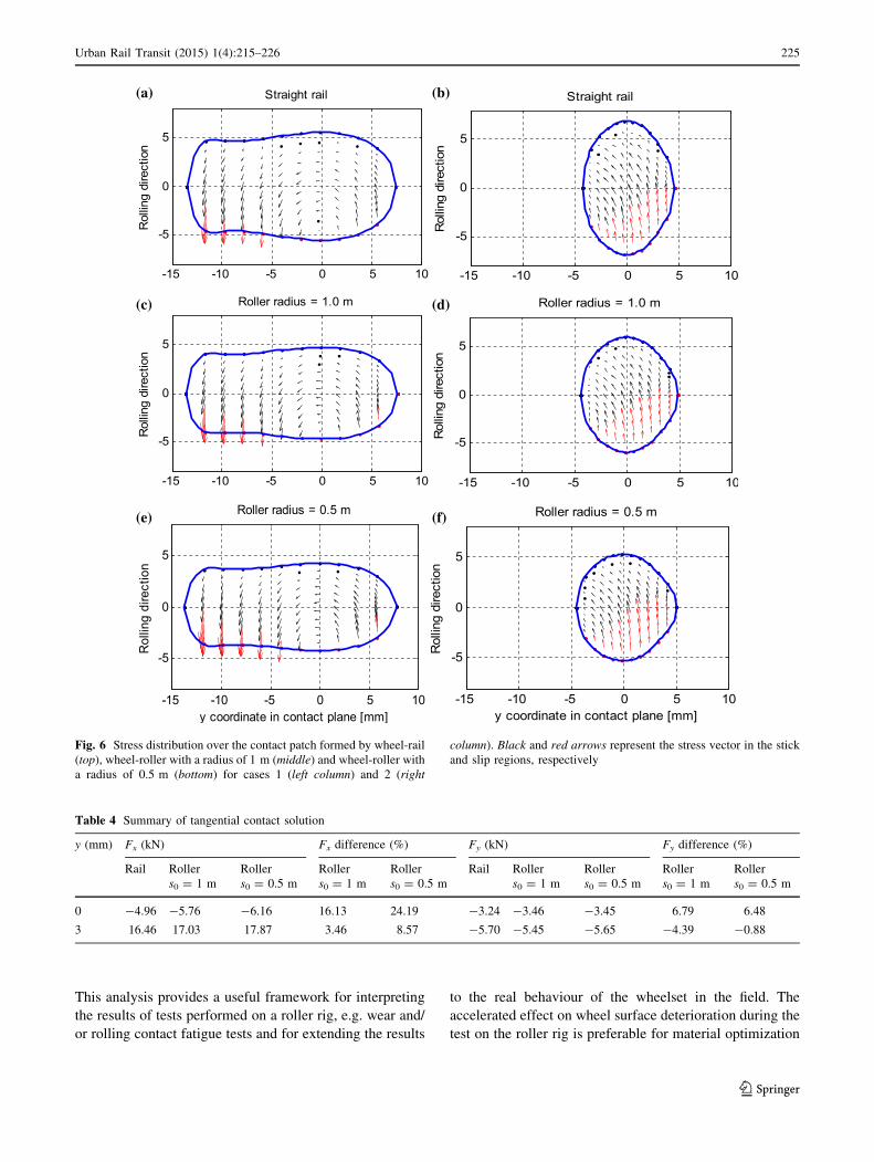
cases introduced in Sect. 4.1 are presented in Fig. 6 in
terms of the stress distribution and division of the contact
patch into a stick region and a slip region.
It can be observed from Fig. 6 that the pattern of the
stress distribution over the contact patch is similar for
wheel-rail and wheel-roller contact conditions in both cases
considered. However, the relative percentage of the slip
region over the whole contact area is slightly larger in the
case of wheel-roller contact. The resultant tangential creep
forces in longitudinal and lateral directions are calculated
by integration over the contact area, and are presented in
Table 4 together with the differences caused by the roller
rig test.
It can be seen from Table 4 that the resultant longitu-
dinal force produced on the roller rig differs significantly
from the same quantity in the wheel-rail contact case when
the contact patch is highly non-elliptic, i.e. for y = 0 mm,
and the difference increases as the radius of roller
decreases, whereas the differences are relative small for
approximately elliptic contact condition, i.e. for
y = 3 mm, especially when the lateral component of the
tangential force is concerned.
To evaluate the contact surface damage situation the
frictional power at the contact patch is calculated for each
case study, and the results are summarized in Table 5.
Table 2 Parameters defining the case studies
No. y (mm) Longitudinal nx Lateral ny Spin nz (m-1)
Rail Roller
s0 = 1 m
Roller
s0 = 0.5 m
Rail Roller
s0 = 1 m
Roller
s0 = 0.5 m
Rail Roller
s0 = 1 m
Roller
s0 = 0.5 m
1 0 0 0 0 0 0 0 0.075 0.109 0.143
2 3 -0.0017 -0.0022 -0.0027 0 0 0 0.197 0.287 0.377
Urban Rail Transit (2015) 1(4):215–226 223
123

It is clear from Table 5 that the frictional power
increases considerably in the case of wheel-roller contact
with respect to wheel-rail contact under the same condi-
tion, and the differences are particularly relevant for a
smaller radius of the roller. It should be noted that the
increase of frictional power implies an accelerated mani-
festation of wear and fatigue effects in the contact pair.
This accelerated effect caused by the roller should be taken
in proper account by wheel-rail surface damage/deteriora-
tion studies performed using roller rigs. It is worth men-
tioning that this accelerated effect is desirable for wheel
material comparison/optimization concerning wear,
because the roller rig is capable of reproducing wear pat-
terns within a much shorter time compared to field testing.
The test results from the roller rig can be used to examine
and document differences in hardening, profile develop-
ment, polygonalization and possible crack formation of the
wheel under test [28]. More details on the wear test on the
roller rig can be found in references [28, 29].
5 Conclusions
This paper investigated the differences between wheel-rail
contact and wheel-roller contact, with the final aim of
assessing the extent to which the results obtained on a
roller rig can be extended to the case of a wheelset running
on a real track.
A systematic description and comparison on the
methodology for solving the contact problem at the wheel-
rail and wheel-roller interfaces have been done in terms of
the geometric contact problem, normal contact problem,
kinematic problem and tangential contact problem. A
modified Kik–Piotrowski model has been proposed to deal
with the wheel-roller contact problem for zero yaw angle
contact conditions.
Simulation results have pointed out the differences
implied by a test performed on a roller rig compared to
wheel-rail contact in terms of size and shape of the contact
patch and distribution of the normal and tangential stresses.
(a) (b)
(c) (d)
Fig. 5 Contact patch (top) and the pressure along its y-axis (bottom) for cases 1 (left column) and 2 (right column)
Table 3 Summary of normal contact solution
y (mm) Contact area Ac (mm2) Ac.difference (%) Max. pressure Pm (MPa) Pm.difference (%)
Rail Roller
s0 = 1 m
Roller
s0 = 0.5 m
Roller
s0 = 1 m
Roller
s0 = 0.5 m
Rail Roller
s0 = 1 m
Roller
s0 = 0.5 m
Roller
s0 = 1 m
Roller
s0 = 0.5 m
0 201 176 159 -12.4 -20.9 598 682 754 14.0 26.1
3 94 84 78 -10.6 -17.0 1336 1498 1632 12.1 22.2
224 Urban Rail Transit (2015) 1(4):215–226
123
This analysis provides a useful framework for interpreting
the results of tests performed on a roller rig, e.g. wear and/
or rolling contact fatigue tests and for extending the results
to the real behaviour of the wheelset in the field. The
accelerated effect on wheel surface deterioration during the
test on the roller rig is preferable for material optimization
(a) (b)
(c) (d)
(e) (f)
Fig. 6 Stress distribution over the contact patch formed by wheel-rail
(top), wheel-roller with a radius of 1 m (middle) and wheel-roller with
a radius of 0.5 m (bottom) for cases 1 (left column) and 2 (right
column). Black and red arrows represent the stress vector in the stick
and slip regions, respectively
Table 4 Summary of tangential contact solution
y (mm) Fx (kN) Fx difference (%) Fy (kN) Fy difference (%)
Rail Roller
s0 = 1 m
Roller
s0 = 0.5 m
Roller
s0 = 1 m
Roller
s0 = 0.5 m
Rail Roller
s0 = 1 m
Roller
s0 = 0.5 m
Roller
s0 = 1 m
Roller
s0 = 0.5 m
0 -4.96 -5.76 -6.16 16.13 24.19 -3.24 -3.46 -3.45 6.79 6.48
3 16.46 17.03 17.87 3.46 8.57 -5.70 -5.45 -5.65 -4.39 -0.88
Urban Rail Transit (2015) 1(4):215–226 225
123

study, while it is not the case for reproducing the wear
process of the wheel in service. In this second case, the
above-mentioned effect must be taken into account when
translating the results of the test to the field case.
Further work will focus on the development of a contact
model which is capable of taking into account the influence
of yaw angle for both normal and tangential problems.
Open Access This article is distributed under the terms of the
Creative Commons Attribution 4.0 International License (http://crea
tivecommons.org/licenses/by/4.0/), which permits unrestricted use,
distribution, and reproduction in any medium, provided you give
appropriate credit to the original author(s) and the source, provide a
link to the Creative Commons license, and indicate if changes were
made.
References
1. Keylin A, Ahmadian M (2012) Wheel-rail contact characteristics
on a tangent track vs a roller rig. In: Proceedings of the ASME
2012 rail transportation division fall technical conference, Omaha
2. Jaschinski A, Chollet H, Iwnicki S, Wickens AH, Wurzen JV
(1999) The application of the roller rigs to railway vehicle
dynamics. Veh Syst Dyn 31:345–392
3. Meymand SZ, Craft MJ, Ahmadian M (2013) On the application
of roller rigs for studying rail vehicle systems. In: Proceedings of
the ASME 2013 rail transportation division fall technical con-
ference, Altoona
4. Zhang W, Dai H, Shen Z, Zeng J (2006) Roller rigs. In: Iwnicki S
(ed) Handbook of railway vehicle dynamics. Taylor & Francis
Group, Boca Raton, pp 458–504
5. Allen PD (2006) Scaling testing. In: Iwnicki S (ed) Handbook of
railway vehicle dynamics. Taylor & Francis Group, Boca Raton,
pp 507–525
6. Yan M (1993) A study of the inherent errors in a roller rig model
of railway vehicle dynamic behaviour. ME thesis, Manchester
Metropolitan University
7. Taheri M, Ahmadian M (2012) Contact patch comparison
between a roller rig and tangent track for a single wheelset. In:
Proceedings of the 2012 joint rail conference, Philadelphia
8. Zeng Y, Shu X, Wang C, Yu W (2013) Study on three-dimen-
sional wheel/rail contact geometry using generalized projection
contour method. In: Zhang W (ed) proceedings of the IAVSD
2013 international symposium on dynamics of vehicles on roads
and tracks, Qingdao
9. Bruni S, Cheli F, Resta F (2001) A model of an actively con-
trolled roller rig for tests on full size wheelsets. Proc Inst Mech
Eng Part F: J Rail Rapid Transit 215:277–288
10. Liu B, Bruni S (2015) A method for testing railway wheel sets on
a full-scale roller rig. Veh Syst Dyn 53(9):1331–1348
11. Shabana AA, Zaazaa KE, Sugiyama H (2007) Railroad vehicle
dynamics: a computational approach. Taylor & Francis Group,
LLC, Boca Raton
12. Bosso N, Spiryagin M, Gugliotta A, Soma A (2013) Mechatronic
modeling of real-time wheel-rail contact. Springer, London
13. Kalker JJ (1982) A fast algorithm for the simplified theory of
rolling contact. Veh Syst Dyn 11:1–13
14. PomboJ Ambrosio J, Silva M (2007) A new wheel-rail contact
model for railway dynamics. Veh Syst Dyn 45(2):165–189
15. Yang G (1993) Dynamic analysis of railway wheelsets and
complete vehicle systems. Doctoral dissertation, Delft University
of technology, Delft
16. Hertz H (1882) Uber die beruhrung fester elastische korper. J Fur
Die Reine U Angew Math 92:156–171
17. Damme S, Nackenhorst U, Wetzel A, Zastrau B (2002) On the
numerical analysis of the wheel-rail system in rolling contact. In:
Popp S (ed): system dynamics and long-term behaviour of rail-
way vehicles, track and subgrade. Lecture Notes in applied
mechanics, vol 6, Springer-Verlag, Berlin, pp 155–174
18. Vo KD, Zhu HT, Tieu AK, Kosasih PB (2015) FE method to
predict damage formation on curved track for various worn status
of wheel/rail profiles. Wear V322–323:61–75
19. Kalker JJ (1990) Three-dimensional elastic bodies in rolling
contact. Solid mechanics and its applications. Kluwer Academic
Publishers, Dordrecht
20. Knothe K, Le The H (1984) A contribution to calculation of
contact stress distribution between elastic bodies of revolution
with non-elliptical contact area. Comput Struct 18(6):1025–1033
21. Kik W, Piotrowski J (1996) A fast, approximate method to cal-
culate normal load at contact between wheel and rail and creep
forces during rolling. In: Zobory I (ed.), proceedings of 2nd mini-
conference on contact mechanics and wear of rail/wheel systems,
Budapest
22. Piotrowski J, Chollet H (2005) Wheel–rail contact models for
vehicle system dynamics including multi-point contact. Veh Syst
Dyn 43(6–7):455–483
23. Piotrowski J, Kik W (2008) A simplified model of wheel/rail
contact mechanics for non-Hertzian problems and its application
in rail vehicle dynamic simulations. Veh Syst Dyn 46(2):27–48
24. Ayasse J, Chollet H (2005) Determination of the wheel rail
contact patch in semi-Hertzian conditions. Veh Syst Dyn
43:161–172
25. Linder Ch (1997) Verschleiss von Eisenbahnradern mit
Unrundheiten. Diss. Techn. Wiss. ETH Zurich, Nr. 12342
26. Sichani MS, Enblom R, Berg M (2014) Comparison of non-el-
liptic contact models: towards fast and accurate modelling of
wheel–rail contact. Wear 314:111–117
27. Vollebregt EAH, Wilders P (2011) FASTSIM2: a second-order
accurate frictional rolling contact algorithm. Comput Mech
47:105–116
28. Ullrich D, Luke M (2001) Simulating rolling-contact fatigue and
wear on a wheel/rail simulation test rig. World Congress on
Railway Research, Cologne
29. Braghin F, Bruni S, Resta F (2001) Wear of railway wheel pro-
files: a comparison between experimental results and a mathe-
matical model. In: Ture H (ed.), 17th international symposium on
dynamics of vehicles on roads and tracks, pp 478–489
Table 5 Frictional power y (mm) Frictional power Pf (Nm/s) Pf.difference (%)
Rail Roller s0 = 1 m Roller s0 = 0.5 m Roller s0 = 1 m Roller s0 = 0.5 m
0 72.41 116.59 200.94 61.01 177.50
3 608.50 847.42 1119.02 39.26 83.90
226 Urban Rail Transit (2015) 1(4):215–226
123