Analysis of Variance: The Fundamental Conceptsjmmtonline.com/documents/v17n2/sawyer.pdf · statistics textbooks, ... ear regression and general linear models ... ABSTRACT: Analysis

The Journal of Manual & ManipulaTive Therapy n voluMe 17 n nuMber 2 [e27]

Department of Rehabilitation Sciences, School of Allied Health Sciences,Texas Tech University Health Sciences Center, Lubbock, TXAddress all correspondence and requests for reprints to: Steven F. Sawyer, PT, PhD, [email protected]

Analysis of variance (ANOVA) is a statistical tool used to detect differ-ences between experimental group

means. ANOVA is warranted in experi-mental designs with one dependent vari-able that is a continuous parametric nu-merical outcome measure, and multiple experimental groups within one or more independent (categorical) variables. In ANOVA terminology, independent vari-ables are called factors, and groups within each factor are referred to as levels. The array of terms that are part and parcel of ANOVA can be intimidating to the un-initiated, such as: partitioning of vari-ance, main effects, interactions, factors, sum of squares, mean squares, F scores, familywise alpha, multiple comparison

procedures (or post hoc tests), effect size, statistical power, etc. How do these terms pertain to p values and statistical signifi-cance? What precisely is meant by a “sta-tistically significant ANOVA”? How does analyzing variance result in an inferential decision about differences in group means? Can ANOVA be performed on non-parametric data? What are the vir-tues and potential pitfalls of ANOVA? These are the issues to be addressed in this primer on the use and interpretation of ANOVA. The intent is to provide the clinician reader, whose misspent youth did not include an enthusiastic reading of statistics textbooks, an understanding of the fundamentals of this widely used form of inferential statistical analysis.

ANOVA General Linear Models

ANOVA is based mathematically on lin-ear regression and general linear models that quantify the relationship between the dependent variable and the indepen-dent variable(s)1. There are three different general linear models for ANOVA: (i) Fixed effects model (Model 1) makes infer-ences that are specific and valid only to the populations and treatments of the study. For example, if three treatments involve three different doses of a drug, inferential conclusions can only be drawn for those specific drug doses. The levels within each factor are fixed as defined by the experimental design. (ii) Random ef-fects model (Model 2) makes inferences about levels of the factor that are not used in the study, such as a continuum of drug doses when the study only used three doses. This model pertains to random ef-fects within levels, and makes inferences about a population’s random variation. (iii) Mixed effects model (Model 3) con-tains both Fixed and Random effects.

In most types of orthopedic reha-bilitation clinical research, the Fixed ef-fects model is relevant since the statistical inferences being sought are fixed to the levels of the experimental design. For this reason, the Fixed effects model will be the focus of this article. Computer statistics programs typically default to the Fixed effects model for ANOVA analysis, but higher end programs can perform ANOVA with all three models.

ABSTRACT: Analysis of variance (ANOVA) is a statistical test for detecting differences in group means when there is one parametric dependent variable and one or more indepen-dent variables. This article summarizes the fundamentals of ANOVA for an intended benefit of the clinician reader of scientific literature who does not possess expertise in statistics. The emphasis is on conceptually-based perspectives regarding the use and interpretation of ANOVA, with minimal coverage of the mathematical foundations. Computational exam-ples are provided. Assumptions underlying ANOVA include parametric data measures, normally distributed data, similar group variances, and independence of subjects. However, normality and variance assumptions can often be violated with impunity if sample sizes are sufficiently large and there are equal numbers of subjects in each group. A statistically sig-nificant ANOVA is typically followed up with a multiple comparison procedure to identify which group means differ from each other. The article concludes with a discussion of effect size and the important distinction between statistical significance and clinical significance.

KEYWORDS: Analysis of Variance, Interaction, Main Effects, Multiple Comparison Procedures

Analysis of Variance: The Fundamental ConceptsSteven F. Sawyer, PT, PhD

[e28] The Journal of Manual & ManipulaTive Therapy n voluMe 17 n nuMber 2

AnAlysis oF VAriAnCe: The FundAmenTAl ConCepTs

Assumptions of ANOVA

Assumptions for ANOVA pertain to the underlying mathematics of general lin-ear models. Specifically, a data set should meet the following criteria before being subjected to ANOVA:

Parametric data: A parametric ANOVA, the topic of this article, re-quires parametric data (ratio or interval measures). There are non-parametric, one-factor versions of ANOVA for non-parametric ordinal (ranked) data, spe-cifically the Kruskal-Wallis test for inde-pendent groups and the Friedman test for repeated measures analysis.

Normally distributed data within each group: ANOVA can be thought of

as a way to infer whether the normal dis-tribution curves of different data sets are best thought of as being from the same population or different populations (Figure 1). It follows that a fundamental assumption of parametric ANOVA is that each group of data (each level) be normally distributed. The Shapiro-Wilk test2 is commonly used to test for nor-mality for group sample sizes (N) less than 50; D’Agnostino’s modification3 is useful for larger samplings (N>50).

A normal distribution curve can be described by whether it has symmetry about the mean and the appropriate width and height (peakedness). These attributes are defined statistically by “skewness” and “kurtosis”, respectively.

A normal distribution curve will have skewness = 0 and kurtosis = 3. (Note that an alternative definition of kurtosis sub-tracts 3 from the final value so that a normal distribution will have kurtosis = 0. This “minus 3” kurtosis value is some-times referred to as “excess kurtosis” to distinguish it from the value obtained with the standard kurtosis function. The kurtosis value calculated by many statis-tical programs is the “minus 3” variant but is referred to, somewhat mislead-ingly, as “kurtosis.”). Normality of a data set can be assessed with a z-test in refer-ence to the standard error of skewness (estimated as √[6 / N) and the standard error of kurtosis (estimated as √[24 / N)4. A conservative alpha of 0.01 (z ≥

FIGURE 1. Graphical representation of statistical Null and Alternative hypotheses for ANOVA in the case of one dependent variable (change in ankle ROM pre/post manual therapy treatment, in units of degrees), and one independent variable with three levels (three different types of manual therapy treatments). For this fictitious data, the group (sample) means are 13, 14 and 18 degrees of increased ankle ROM for treatment type groups 1, 2 and 3, respectively (raw data are presented in Figure 2). The Null hypothesis is represented in the left graph, in which the population means for all three groups are assumed be identical to each other (in spite of difference in sample means calculated from the experimental data). Since in the Null hypothesis the subjects in the three groups are considered to compose a single population, by definition the population means of each group are equal to each other, and are equal to the Grand mean (mean for all data scores in the three groups). The corresponding normal distribution curves are identical and precisely overlap along the X-axis. The Alternative hypothesis is shown in right graph, in which differences in group sample means are inferred to represent true differences in group population means. These normal distribution curves do not overlap along the X-axis because each group of subjects are considered to be distinct populations with respect to ankle ROM, created from the original single population that experienced different efficacies of the three treatments. Graph is patterned after Wilkinson et al11.

pro

bab

ility

den

sity

Fu

nct

ion

pro

bab

ility

den

sity

Fu

nct

ion

AnoVA null hypothesis: identical normal distribution curve

AnoVA null hypothesis: different normal distribution curve

increased elbow rom (degree) increased elbow rom (degree)



2.56) is appropriate, due to the overly sensitive nature of these tests, especially for large sample sizes (>100)4. As a com-putational example, for N = 20, the esti-mation of standard error of skewness = √[6 / 20] = 0.55, and any skewness value greater than ±2.56 x 0.55 = ±1.41 would indicate non-normality. Perhaps the best “test” is what always should be done: examine a histogram of the distri-bution of the data. In practice, any dis-tribution that resembles a bell-shaped curve will be “normal enough” to pass normality tests, especially if the sample size is adequate.

Homogeneity of variance within each group: Referring again to the notion that ANOVA compares normal distri-bution curves of data sets, these curves need to be similar to each other in shape and width for the comparison to be valid. In other words, the amount of data dispersion (variance) needs to be similar between groups. Two commonly in-voked tests of homogeneity of variance are by Levene5 and Brown & Forsthye6.

Independent Observations: A gen-eral assumption of parametric analysis is that the value of each observation for each subject is independent of (i.e., not related to or influenced by) the value of any other observation. For independent groups designs, this issue is addressed with random sampling, random assign-ment to groups, and experimental con-trol of extraneous variables. This as-sumption is an inherent concern for repeated measures designs, in which an assumption of sphericity comes into play. When subjects are exposed to all levels of an independent variable (e.g., all treatments), it is conceivable that the effects of a treatment can persist and af-fect the response to subsequent treat-ments. For example, if a treatment effect for one level has a long half-time (analo-gous to a drug effect) and there is inad-equate “wash out” time between expo-sure to different levels (treatments), there will be a carryover effect. A well designed and executed cross-over ex-perimental design can mitigate carry-over effects. Mauchly’s test of sphericity is commonly employed to test the as-sumption of independence in repeated measures designs. If the Mauchly test is statistically significant, corrections to

the F score calculation are warranted. The two most commonly used correc-tion methods are the Greenhouse-Geisser and Huynh-Feldt, which calcu-late a descriptive statistic called epsilon, which is a measure of the extent to which sphericity has been violated. The range of values for epsilon are 1 (no sphericity violation) to a lower boundary of 1 / (m—1), where m = number of levels. For example, with three groups, the range would be 1 to 0.50. The closer epsilon is to the lower boundary, the greater the degree of violation. There are three op-tions for adjusting the ANOVA to ac-count for the sphericity violation, all of which involve modifying degrees of freedom: use the lower boundary epsi-lon, which is the most conservative ap-proach (least powerful) and will gener-ate the largest p value, or use either the Greenhouse-Geisser epsilon or the Huynh-Feldt epsilon (most powerful) [statistical power is the ability of an in-ferential test to detect a difference that actually exists, i.e., a true positive].

Most commercially available statis-tics programs perform normality, ho-mogeneity of variance and sphericity tests. Determination of the parametric nature of the data and soundness of the experimental design is the responsibility of the investigator, reviewers and critical readers of the literature.

Robustness of ANOVA to Violations of Normality and Variance Assumptions

ANOVA tests can handle moderate vio-lations of normality and equal variance if there is a large enough sample size and a balanced design7. As per the central limit theorem, the distribution of sam-ple means approximates normality even with population distributions that are grossly skewed and non-normal, so long as the sample size of each group is large enough. There is no fixed definition of “large enough”, but a rule of thumb is N≥308. Thus, the mathematical validity of ANOVA is said to be “robust” in the face of violations of normality assump-tions if there is an adequate sample size. ANOVA is more sensitive to violations of the homogeneity of variance assump-tion, but this is mitigated if sample sizes of factors and levels are equal or nearly

so9,10. If normality and homogeneity of variance violations are problematic, there are three options: (i) Mathemati-cally transform (log, arcsin, etc.) the data to best mitigate the violation, with the cost of cognitive fog in understand-ing the meaning to the ANOVA results (e.g., “A statistically significant main ef-fect was obtained for the arcsin transfor-mation of degrees of ankle range of mo-tion”). (ii) Use one of the non-parametric ANOVAs mentioned above, but at the cost of reduced power and being limited to one-factor analysis. (iii) Identify out-liers in the data set using formal statisti-cal criteria (not discussed here). Use caution in deleting outliers from the data set; such decisions need to be justi-fied and explained in research reports. Removal of outliers will reduce devia-tions from normality and homogeneity of variance.

If You Understand t-Tests, You Already Know A Lot About ANOVA

As a starting point, the reader should understand that the familiar t-test is an ANOVA in abbreviated form. A t-test is used to infer on statistical grounds whether there are differences between group means for an experimental design with (i) one parametric dependent vari-able and (ii) one independent variable with two levels, i.e., there is one outcome measure and two groups. In clinical re-search, levels often correspond to differ-ent treatment groups; the term “level” does not imply any ordering of the groups.

The Null statistical hypothesis for a t-test is H0: μ1 = μ2, that is, the population means of the two groups are the same. Note that we are dealing with popula-tion means, which are almost always unknown and unknowable in clinical research. If the Null hypothesis involved sample means, there would be nothing to infer, since descriptive analysis pro-vides this information. However, with inferential analysis using t-tests and ANOVA, the aim is to infer, without ac-cess to “the truth”, if the group popula-tion means differ from each other.

The Alternative hypothesis, which comes into play if the Null hypothesis is rejected, asserts that the group popula-



tion means differ. The Null hypothesis is rejected when the p value yielded by the t-test is less than alpha. Alpha is the pre-determined upper limit risk for commit-ting a Type 1 error, which is the statisti-cal false positive of incorrectly rejecting the Null hypothesis and inferring the groups means differ when in fact the groups are from a single population. By convention, alpha is typically set to 0.05. The p value generated by the t-test statis-tic is based on numerical analysis of the experimental data, and represents the probability of committing a Type 1 error if the Null hypothesis is rejected. When p is less than alpha, there is a statistically significant result, i.e., the values in the two groups are inferred to differ from each other and to represent separate populations. The logic of statistical in-ference is analogous to a jury trial: at the outset of the trial (inferential analysis), the group data are presumed to be in-nocent of having different population means (Null hypothesis) unless the dif-ferences in group means in the sampled data are sufficiently compelling to meet the standard of “beyond a reasonable doubt” (p less than alpha), in which case a guilty verdict is rendered (reject Null hypothesis and accept Alternative hy-pothesis = statistical significance).

The test statistic for a t-test is the t score. In conceptual terms, the calcula-tion of a t score for independent groups (i.e., not repeated measures) is as fol-lows:

t = statistical signal / statistical noiset = treatment effect / unexplained vari-

ance (“error variance”)t = differences between sample means

of the two groups / within-group variance

The difference in group means repre-sents the statistical signal since it is pre-sumed to result from treatment effects of the different levels of the independent variable. The within-group variance is considered to be statistical noise and an “error” term because it is not explained by the influence of the independent vari-able on the dependent variable. The par-ticulars of how the t score is calculated depends on the experimental design (in-dependent groups vs repeated measures)

and whether variance between groups is equivalent; the reader is to referred to any number of statistics books for details about the formulae. The t score is con-verted into a p value based on the magni-tude of the t score (larger t scores lead to smaller p values) and the sample size (which relates to degrees of freedom).

ANOVA Null Hypothesis and Alternative Hypothesis

ANOVA is applicable when the aim is to infer differences in group values when there is one dependent variable and more than two groups, such as one inde-pendent variable with three or more lev-els, or when there are two or more inde-pendent variables. Since an independent variable is called a “factor”, ANOVAs are described in terms of the number of fac-tors; if there are two independent vari-ables, it is a two-factor ANOVA. In the simpler case of a one-factor ANOVA, the Null hypothesis asserts that the pop-ulation means for each level (group) of the independent variable are equal. Let’s use as an example a fictitious experi-ment with one dependent variable (pre/post changes in ankle range of motion in subjects who received one of three types of manual therapy treatment after surgi-cal repair of a talus fracture). This con-stitutes a one-factor ANOVA with three levels (the three different types of treat-ment). The Null hypothesis is: H0: μ1 = μ2 = μ3. The Alternative hypothesis is that at least two of group means differ. Figure 1 provides a graphical presentation of this ANOVA statistical hypotheses: (i) the Null hypothesis (left graph) asserts that the normal distribution curves of data for the three groups are identical in shape and position and therefore pre-cisely overlap, whereas (ii) the Alterna-tive hypothesis (right graph) asserts that these normal distribution curves are best described by the distribution indi-cated by the sample means, which repre-sent an experimentally-derived estimate of the population means11.

The Mechanics of Calculating a One-factor ANOVA

ANOVA evaluates differences in group means in a round-about fashion, and

involves the “partitioning of variance” from calculations of “Sum of Squares” and “Mean Squares.” Three metrics are used in calculating the ANOVA test sta-tistic, which is called the F score (named after R.A. Fisher, the developer of ANOVA): (i) Grand Mean, which is the mean of all scores in all groups; (ii) Sum of Squares, which are of two kinds, the sum of all squared differences between group means and the Grand Mean (be-tween-groups Sum of Squares) and the sum of squared differences between in-dividual data scores and their respective group mean (within-groups Sum of Squares), and (iii) Mean Squares, also of two kinds (between-groups Mean Squares, within-groups Mean Squares), which are the average deviations of indi-vidual scores from their respective mean, calculated by dividing Sum of Squares by their appropriate degrees of freedom.

A key point to appreciate about ANOVA is that the data set variance is partitioned into statistical signal and statistical noise components to generate the F score. The F score for independent groups is calculated as:

F = statistical signal / statistical noiseF = treatment effect / unexplained vari-

ance (“error variance”)F = Mean SquaresBetween Groups / Mean

SquaresWithin Groups (Error)

Note that the statistical signal, the MSBe-

tween Groups term, is an indirect measure of differences in group means. The MSWithin

Groups (Error) term is considered to represent statistical noise/error since this variance is not explained by the effect of the inde-pendent variable on the dependent vari-able. Here is the gist of the issue: as group means increasingly diverge from each other, there is increasingly more variance for between-group scores in re-lation to the Grand Mean, quantified as Sum of SquaresBetween Groups, leading to a larger MSBetween Groups term and a larger F score. Conversely, as there is more vari-ance within-group scores, quantified as Sum of SquaresWithin Groups (Error), the MSWithin Groups (Error) term will increase, leading to a smaller F score. Thus, for independent groups, large F scores arise from large differences between group



means and/or small variances within groups. Larger F scores equate to lower p values, with the p value also influenced by the sample size and number of groups, each of which constitutes separate types of “degrees of freedom.”

ANOVA calculations are now the domain of computer software, but there is illustrative and heuristic value in man-ually performing the arithmetic calcula-tion of the F score to garner insight into how analysis of data set variance gener-ates a statistical inference about differ-ences in group means. A numerical ex-ample is provided in Figure 2, in which the data set graphed in Figure 1 is listed

and subjected to ANOVA, yielding a cal-culated F score and corresponding p value.

Mathematical Equivalence of t-tests and ANOVA: t-tests are a Special Case

of ANOVA

Let’s briefly return to the notion that a t-test is a simplified version of ANOVA that is specific to the case of one inde-pendent variable with two groups. If we analyze the data in Figure 2 for the Type 1 treatment vs. Type 3 treatment group data (disregarding the Type 2 treatment group data to reduce the analysis to two

groups), the t score for independent groups is 5.0 with a p value of 0.0025 (calculations not shown). For the same data assessed with ANOVA, the F score is 25.0 with a p value of 0.0025. The t-test and ANOVA generate identical p values. The mathematical relation between the two test statistics is: t2 = F.

Repeated Measures ANOVA: Different Error Term, Greater Statistical Power

The experimental designs emphasized thus far entail independent groups, in which each subject is “exposed” to only one level of an independent variable. In

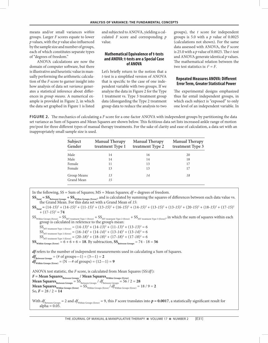
FIGURE 2. The mechanics of calculating a F score for a one-factor ANOVA with independent groups by partitioning the data set variance as Sum of Squares and Mean Squares are shown below. This fictitious data set lists increased ankle range of motion pre/post for three different types of manual therapy treatments. For the sake of clarity and ease of calculation, a data set with an inappropriately small sample size is used.

Subject Manual Therapy Manual Therapy Manual Therapy Gender treatment Type 1 treatment Type 2 treatment Type 3

Male 14 16 20Male 14 14 18Female 11 13 17Female 13 13 17

Group Means 13 14 18Grand Mean 15

In the following, SS = Sum of Squares; MS = Mean Squares; df = degrees of freedom.SSTotal = SSBetween Groups + SSWithin Groups (Error), and is calculated by summing the squares of differences between each data value vs.

the Grand Mean. For this data set with a Grand Mean of 15:SSTotal = (14-15)2 + (14-15)2 + (11-15)2 + (13-15)2 + (16-15)2 + (14-15)2 + (13-15)2 + (13-15)2 + (20-15)2 + (18-15)2 + (17-15)2

+ (17-15)2 = 74SSWithin Groups (Error) = SSMT treatment Type 1 (Error) + SSMT treatment Type 2 (Error) + SSMT treatment Type 3 (Error), in which the sum of squares within each

group is calculated in reference to the group’s mean: SSMT treatment Type 1 (Error) = (14-13)2 + (14-13)2 + (11-13)2 + (13-13)2 = 6 SSMT treatment Type 2 (Error) = (16-14)2 + (14-14)2 + (13-14)2 + (13-14)2 = 6 SSMT treatment Type 3 (Error) = (20-18)2 + (18-18)2 + (17-18)2 + (17-18)2 = 6SSWithin Groups (Error) = 6 + 6 + 6 = 18. By subtraction, SSBetween Groups = 74 - 18 = 56

df refers to the number of independent measurements used in calculating a Sum of Squares.dfBetween Groups = (# of groups—1) = (3—1) = 2dfWithin Groups (Error) = (N —# of groups) = (12—1) = 9

ANOVA test statistic, the F score, is calculated from Mean Squares (SS/df ):F = Mean SquaresBetween Groups / Mean SquaresWithin Groups (Error)Mean SquaresBetween Groups = SSBetween Groups / dfBetween Groups = 56 / 2 = 28Mean SquaresWithin Groups (Error) = SSWithin Groups (Error) / dfWithin Groups (Error) = 18 / 9 = 2So, F = 28 / 2 = 14

With dfBetween Groups = 2 and dfWithin Groups (Error) = 9, this F score translates into p = 0.0017, a statistically significant result for alpha = 0.05.



the data set of Figure 2, this would in-volve each subject receiving only one of the three different treatments. If a sub-ject is exposed to all levels of an inde-pendent variable, the mechanics of the ANOVA are altered to take into account that each subject serves as their own ex-perimental control. Whereas the term for statistical signal, MSBetween Groups, is un-changed, there is a new statistical noise term called MSWithin Subjects (Error) that per-tains to variance within each subject across all levels of the independent vari-able instead of between all subjects within one level. Since there is typically less variation within subjects than be-tween subjects, the statistical error term is typically smaller in repeated measures designs. A smaller MSWithin Subjects (Error) value leads to a larger F value and a smaller p value. As a result, repeated measures ANOVA typically have greater statistical power than independent groups ANOVA.

Factorial ANOVA: Main Effects and Interactions

An advantage of ANOVA is its ability to analyze an experimental design with multiple independent variables. When an ANOVA has two or more indepen-dent variables it is referred to as a facto-r ial ANOVA, in contrast to the one- factor ANOVAs discussed thus far. This is efficient experimentally, because the effects of multiple independent variables on a dependent variable are tested on one cohort of subjects. Furthermore, factorial ANOVA permits, and requires, an evaluation of whether there is an in-terplay between different levels of the independent variables, which is called an interaction.

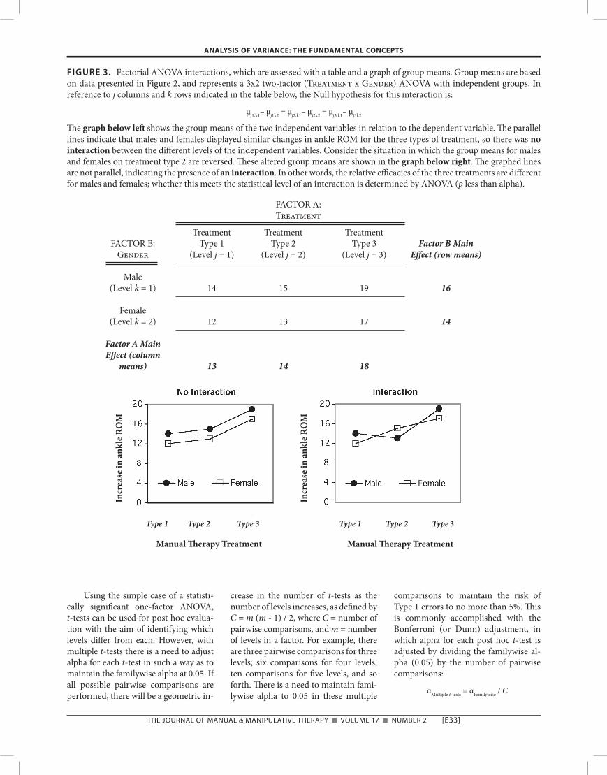
Definitions of terminology that is unique to factorial ANOVA are war-ranted: (i) Main effect is the effect of an independent variable (a factor) on a de-pendent variable, determined separate from of the effects of other independent variables. A main effect is a one-factor ANOVA that is performed on a factor that disregards the effects of other fac-tors. In a two factor ANOVA, there are two main effects, one for each indepen-dent variable; a three-factor ANOVA has three main effects, and so on. (ii) In-

teraction describes an interplay between independent variables such that differ-ent levels of the independent variables have non-additive effects on the depen-dent variable. In formal terms, there is an interaction between two factors when the dependent variable response at levels of one factor differ from those produced at levels of the other factor(s). Interactions can be easily identified in graphs of group means. For example, again referring to the data set from Fig-ure 2, let us now consider the effect of subject gender as a second independent variable. This would be a two factor ANOVA: one factor is the sex of sub-jects, called Gender, with two levels; the second factor is the type of manual therapy treatment, called Treatment, with three levels. A shorthand descrip-tion of this design is 2x3 ANOVA (two factors with two and three levels, re-spectively). For this two-factor ANOVA, there are three Null hypotheses: (i) Main Effect for the Gender factor: Are there differences in the response (ankle range of motion) for males vs. females to manual therapy treatment (combin-ing data for the three levels of the Treatment factor with respect to the two Gender factor levels)? (ii) Main Ef-fect for the Treatment factor: Are there differences in the response for subjects in the three levels of the Treat-ment factor (combining data for males and females in the Gender factor with respect to the three Treatment factor levels)? (iii) Interaction: Are there dif-ferences due to neither the Gender or Treatment factors alone but to the combination of these factors? With re-spect to analysis of interactions, Figure 3 shows a table of group means for all levels the two independent variables, based on data from Figure 2. Note that the two independent variables are graphed in relation to the dependent variable. The two lines in the left graph are parallel, indicating the absence of an interaction between the levels of the two factors. An interaction would exist if the graphs were not parallel, such as in the right graph in which group means for males and females on the Type 2 treat-ment were switched for illustrative pur-poses. If the lines deviate from parallel to a sufficient degree, the interaction

will be statistically significant. In this case with two factors, there is only one interaction to be evaluated. With three or more independent variables, there are multiple interactions that need to be considered. A statistically significant in-teraction complicates the interpretation of the Main Effects, since the factors are not independent of each other in their effects on the dependent variable. Inter-actions should be examined before Main Effects. If interactions are not sta-tistically sig nificant, then Main Effects can be easily evaluated as a series of one-factor ANOVAs.

So There is a Statistically Significant ANOVA—Now What? Multiple

Comparison Procedures

If an ANOVA does not yield statistical significance on any main effects or inter-actions, the Null hypothesis (hypothe-ses) is (are) accepted, meaning that the different levels of independent variables did not have any differential effects on the dependent variable. The inferential statistical work is done (but see next sec-tion), unless confounding covariates are suspected, possibly warranting analysis of covariance (ANCOVA), which is be-yond the scope of this article.

When statistical significance is ob-tained in an ANOVA, additional statisti-cal tests are necessary to determine which of the group means differ from each other. These follow-up tests are re-ferred to as multiple comparison proce-dures (MCPs) or post hoc tests. MCPs involve multiple pair-wise comparisons (or contrasts) in a fashion designed to maintain alpha for the family of com-parisons to a specified level, typically 0.05. This is referred to as the familywise alpha. There are two general options for MCP tests: either perform multiple t-tests that require “manual” adjustment of the alpha for each pairwise test to maintain a familywise alpha of 0.05, or use a test such as the Tukey HSD (see below) that has built-in protection from alpha inflation. Multiple t-tests have their place, especially when only a sub-set of all possible pairwise comparisons are to be performed, but the special pur-pose MCPs are preferable when all pair-wise comparisons are assessed.



Using the simple case of a statisti-cally significant one-factor ANOVA, t-tests can be used for post hoc evalua-tion with the aim of identifying which levels differ from each. However, with multiple t-tests there is a need to adjust alpha for each t-test in such a way as to maintain the familywise alpha at 0.05. If all possible pairwise comparisons are performed, there will be a geometric in-

crease in the number of t-tests as the number of levels increases, as defined by C = m (m - 1) / 2, where C = number of pairwise comparisons, and m = number of levels in a factor. For example, there are three pairwise comparisons for three levels; six comparisons for four levels; ten comparisons for five levels, and so forth. There is a need to maintain fami-lywise alpha to 0.05 in these multiple

comparisons to maintain the risk of Type 1 errors to no more than 5%. This is commonly accomplished with the Bonferroni (or Dunn) adjustment, in which alpha for each post hoc t-test is adjusted by dividing the familywise al-pha (0.05) by the number of pairwise comparisons:

αMultiple t-tests = αFamilywise / C

FIGURE 3. Factorial ANOVA interactions, which are assessed with a table and a graph of group means. Group means are based on data presented in Figure 2, and represents a 3x2 two-factor (Treatment x Gender) ANOVA with independent groups. In reference to j columns and k rows indicated in the table below, the Null hypothesis for this interaction is:

μj1,k1– μj1k2 = μj2,k1– μj2k2 = μj3,k1– μj3k2

The graph below left shows the group means of the two independent variables in relation to the dependent variable. The parallel lines indicate that males and females displayed similar changes in ankle ROM for the three types of treatment, so there was no interaction between the different levels of the independent variables. Consider the situation in which the group means for males and females on treatment type 2 are reversed. These altered group means are shown in the graph below right. The graphed lines are not parallel, indicating the presence of an interaction. In other words, the relative efficacies of the three treatments are different for males and females; whether this meets the statistical level of an interaction is determined by ANOVA (p less than alpha).

FACTOR A:Treatment

Treatment Treatment Treatment FACTOR B: Type 1 Type 2 Type 3 Factor B Main Gender (Level j = 1) (Level j = 2) (Level j = 3) Effect (row means)

Male (Level k = 1) 14 15 19 16

Female (Level k = 2) 12 13 17 14

Factor A Main Effect (column means) 13 14 18

Type 1 Type 2 Type 3 Type 1 Type 2 Type 3

Manual Therapy Treatment Manual Therapy Treatment

Incr

ease

in a

nkle

RO

M

Incr

ease

in a

nkle

RO

M



If there are two pairwise compari-sons, alpha for each t-test is set to 0.05/2 = 0.25; for three comparisons, alpha is 0.05/3 = 0.0167, and so on. Any pairwise t-test with a p value less than the ad-justed alpha would be considered statis-tically significant. The trade-off for pre-venting familywise alpha inflation is that as the number of comparisons increases, it becomes incrementally more difficult to attain statistical significance due to the lower alpha. Furthermore, the infla-tion of familywise alpha with multiple t-tests is not additive. As a result, Bon-ferroni adjustments overcompensate the alpha adjustment, making this the most conservative (least powerful) of all MCPs. For example, running two t-tests, each with alpha set to 0.05, does not double familywise alpha to 0.10; it in-creases it to only 0.0975. The effects of multiple t-tests on familywise alpha and Type 1 error rate is defined by the fol-lowing formula:

αFamilywise = 1—(1—αMultiple t-tests)C

The overcorrection by the Bonferroni technique becomes more prominent with many pairwise comparisons: exe-cuting 20 t-tests, each with an alpha of 0.05, does not yield a familywise alpha of 20 x 0.05 = 1.00 (i.e., 100% chance of Type 1 error); the value is actually 0.64. There are modifications of the Bonfer-roni adjustment developed by Šidák12 to more accurately reflect the inflation of familywise alpha that result in larger ad-justed alpha levels and therefore in-creased statistical power, but the effects are slight and rarely convert a margin-ally non-significant pairwise compari-son into a statistical significance. For example, with three pairwise compari-sons, the Bonferroni adjusted alpha of 0.167 is increased by only 0.003 to 0.170 with the Šidák adjustment.

The sequential alpha adjustment methods for multiple post hoc t-tests by Holm13 and Hochberg14 provide in-creased power while still maintaining control of the familywise alpha. These techniques permit the assignment of sta-tistical significance in certain situations for which p values are less than 0.05 but do not meet the Bonferroni criterion for significance. The sequential approach by Holm13 and Hochberg14 are called step-

down and step-up procedures, respec-tively. In Hochberg’s step-up procedure with C pairwise comparisons, the t-test p values are evaluated sequentially in de-scending order, with p1 the lowest value and pC the highest. If pC is less than 0.05, all the p values are statistically signifi-cant. If pC is greater than 0.05, that evalu-ation is non-significant, and the next largest p value, pC - 1, is evaluated with a Bonferroni adjusted alpha of 0.05/2 = 0.025. If pC - 1 is significant, then all re-maining p values are significant. Each sequential evaluation leads to an alpha adjustment based on the number of pre-vious evaluations, not on the entire set of possible evaluations, thereby yielding increased statistical power compared to the Bonferroni method. For example, if three p values are 0.07, 0.02 and 0.015, Hochberg’s method evaluates p3 = 0.07 vs alpha = 0.05/1 = 0.05 (non-signifi-cant); then p2 = 0.02 vs. alpha = 0.05/2 = 0.025 (significant); and then p1 = 0.015 vs alpha = 0.05/3 = 0.0167 (significant). Holm’s method performs the inverse se-quence and alpha adjustments, such that the lowest p value is evaluated first with a fully adjusted alpha. In this case: p1 = 0.015 vs alpha = 0.05/3 = 0.0167 (signifi-cant); then p2 = 0.020 vs. alpha = 0.05/2 = 0.025 (significant); and then p3 = 0.070 vs alpha = 0.05/1 = 0.05 (non-signifi-cant). Once Holm’s method encounters non-significance, sequential evaluations end, whereas Hochberg’ method contin-ues testing. For these three p values, the Bonferroni adjustment would find p = 0.015 significant but p = 0.02 to be non-significant. As can be seen, the methods of Hochberg and Holm are less conser-vative and more powerful than Bonfer-roni’s adjustment. Further, Hochberg’s method is uniformly more powerful than Holm’s method15. For example, if there are three pairwise comparisons with p = 0.045, 0.04 and 0.03, all would be significant with Hochberg’s method but none would be with Holm’s method (or Bonferroni’s).

There are many types of MCPs dis-tinct from the t-test approaches de-scribed above16. These tests have “built-in” familywise alpha protection that do not require “manual” adjustment of al-pha. Most of these MCPs calculate a so-called q value for each comparison that

takes into account group mean differ-ences, group variances, and group sam-ple sizes in a fashion similar but not identical to the calculation of t. This q value is compared to a critical value gen-erated from a q distribution (a distribu-tion of differences in sample means). Protection from familywise alpha infla-tion is in the form of a multiplier applied to the critical value. The multiplier in-creases as the number of comparisons increases, thereby requiring greater dif-ferences between group means to attain statistical significance as the number of comparisons is increased. Some MCPs are better than others at balancing statis-tical power and Type 1 errors. By general consensus amongst statisticians, the Fisher Least Significant Difference (LSD) test and the Duncan’s Multiple Range Test are considered to be overly powerful, with too high a likelihood of Type 1 errors (false positives). The Scheffè test is considered to be overly conservative, with too high a likelihood of Type 2 errors (false negatives), but is applicable when group sample sizes are markedly unequal17. The Tukey Hon-estly Significant Difference (HSD) is fa-vored by many statisticians for its bal-ance of statistical power and protection from Type 1 errors. It is worth noting that the power advantage of the Tukey HSD test obtains only when all possible pairwise comparisons are performed. The Student-Newman-Keuls (SNK) test statistic is computed identically to the Tukey HSD, however the critical value is determined differently using a step-wise approach, somewhat like the Holm method described above for t-tests. This makes the SNK test slightly more power-ful than the Tukey HSD test. However, an advantage of the Tukey HSD test is that a variant called Tukey-Kramer HSD test can be used with unbalanced sample size designs, unlike the SNK test. The Dunnett test is useful when planned pairwise tests are restricted to one group (e.g., a control group) being compared to all other groups (e.g., treatment groups).

In summary, (i) the Tukey HSD and Student-Newman-Keuls tests are rec-ommended when performing all pair-wise tests; (2) the Hochberg or Holm se-quential alpha adjustments enhance the power of multiple post hoc t-tests while



maintaining control of familywise alpha; and (3) the Dunnett test is preferred when comparing one group to all other groups.

Break from Tradition: Skip One-Factor ANOVA and Proceed Directly to a MCP

Thus far, the conventional approach to ANOVA and MCPs has been presented, namely, run an ANOVA and if it is not significant, proceed no further; if the ANOVA is significant, then run MCPs to determine which group means differ. However, it has long been held by some statisticians that in certain circum-stances ANOVA can be skipped and that an appropriate MCP is the only neces-sary inferential test. To quote an influen-tial paper by Wilkinson et al18, the ANOVA-followed-by-MCP approach “is usually wrong for several reasons. First, pairwise methods such as Tukey’s honestly significant difference proce-dure were designed to control a family-wise error rate based on the sample size and number of comparisons. Preceding them with an omnibus F test in a stage-wise testing procedure defeats this de-sign, making it unnecessarily conserva-tive.” Related to this perspective is the fact that inferential discrepancies are possible between ANOVA and MCPs, in which one is statistically significant and the other is not. This can occur when p values are near the boundary of alpha. Each MCP has slightly different criteria for statistical significance (based on ei-ther the t or q distribution), and all differ slightly from the criteria of F scores (based on the F distribution). An argu-ment has also been put forth with respect to performing pre-planned MCPs with-out the need for a statistically significant ANOVA in clinical trials19. Nonetheless, the convention remains to perform ANOVA and then MCPs, but MCPs alone are a statistically valid option. ANOVA is especially warranted when there are multiple factors, due to the abil-ity of ANOVA to detect interactions.

Wilkinson et al.18 also reminds re-searchers that it is rarely necessary to perform all pairwise comparisons. Se-lected pre-planned comparisons that are driven by the research hypothesis, and not a subcortical reflex to perform every

conceivable pairwise comparison, will reduce the number of extraneous pair-wise comparisons and false positives, and have the added benefit of increasing statistical power.

ANOVA Effect Size

Effect size is a unitless measure of the magnitude of treatment effects20. For ANOVA, there are two categories of ef-fect size indices: (i) those based on pro-portions of sum of squares (η2, partial η2, ω2), and (ii) those based on a standard-ized difference between group means (such as Cohen’s d)21,22. The latter type of effect size index is useful for power anal-ysis, and will be discussed briefly in the next section. To an ever increasing de-gree, peer review journals are requiring the presentation of effect sizes with de-scriptive summaries of data.

There are three commonly used ef-fect size indices that are based on pro-portions of the familiar sum of squares values that form the foundation of ANOVA computations. The three indi-ces are called eta squared (η2), partial eta squared (partial η2), and omega squared (ω2). These indices range in value from 0 (no effect) to 1 (maximal effect) because they are proportions of variance. These indices typically yield different values for effect size.

Eta squared (η2) is calculated as:η2 = SSBetween Groups / SSTotal

The SSBetween Groups term pertains to the in-dependent variable of interest, whereas SSTotal is based on the entire data set. Spe-cifically, for a factorial ANOVA, SSTotal = [SSBetween Groups for all factors + SSError + all SSInteractions]. As such, the magnitude of η2 for a given factor will be influenced by the number of other independent vari-ables. For example, η2 will tend to be larger in a one-factor design than in a two-factor design because in the latter the SSTotal term will be inflated to include sum of squares arising from the second factor.

Partial eta squared (partial η2) is calculated with respect to the sum of squares associated with the factor of in-terest, not the total sum of squares:

partial η2 = SSBetween Groups / (SSBetween Groups + SSError)

As with the η2 calculation, the SSBetween

Groups numerator term for partial η2 per-tains to the independent variable of in-terest. However, the denominator differs from that of η2. The denominator for partial η2 is not based on the entire data set (SSTotal) but instead on only SSBetween

Groups and SSError for the factor being eval-uated. For a one-factor ANOVA, the sum of square terms are identical for η2 and partial η2, so the values are identical; however, with factorial ANOVA the de-nominator for partial η2 will always be smaller. For this reason, partial η2 is al-ways larger than η2 with factorial ANOVA (unless a factor or interaction has absolutely no effect, as in the case of the interaction in Figure 4, for which both η2 and partial η2 equal 0).

Omega squared (ω2) is based on an estimation of the proportion of variance in the underlying population, in contrast to the η2 and partial η2 indices that are based on proportions of variance in the sample. For this reason, ω2 will always be a smaller value than η2 and partial η2. Application of ω2 is limited to between-subjects designs (i.e., not repeated mea-sures) with equal samples sizes in all groups. Omega squared is calculated as follows:

ω2 = [SSBetween Groups—(dfBetween Groups)*(MSError)] / (SSTotal + MSError)

In contrast to η2, which provides an up-wardly biased estimate of effect size when the sample size is small, ω2 calcu-lates an unbiased estimate23.

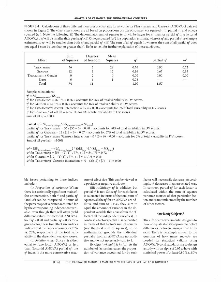
The reader is cautioned that η2and partial η2 are often misreported in the literature (e.g., η2 incorrectly reported as partial η2)24,25. It is advisable to calculate these values by hand using the formulae shown above as a confirmation of the output of statistical software programs, to ensure accurate reporting. Refer to Figure 4 for sample calculations of these three effect size indices for a two-factor ANOVA.

The η2 and partial η2 indices have distinctly different attributes. Whether a given attribute is considered to be an ad-vantage or disadvantage is a matter of perspective and context. Some authors24 argue the merits of eta squared, whereas others4 prefer partial eta squared. Nota-



ble issues pertaining to these indices include:

(i) Proportion of variance: When there is a statistically significant main ef-fect or interaction, both η2 and partial η2 (and ω2) can be interpreted in terms of the percentage of variance accounted for by the corresponding independent vari-able, even though they will often yield different values for factorial ANOVAs. So if η2 = 0.20 and partial η2 = 0.25 for a given factor, these two effect size indices indicate that the factor accounts for 20% vs. 25%, respectively, of the total vari-ability in the dependent variable scores.

(ii) Relative values: Since η2 is either equal to (one-factor ANOVA) or less than (factorial ANOVA) partial η2, the η2 index is the more conservative mea-

sure of effect size. This can be viewed as a positive or negative attribute.

(iii) Additivity: η2 is additive, but partial η2 is not. Since η2 for each factor is calculated in terms of the total sum of squares, all the η2 for an ANOVA are ad-ditive and sum to 1 (i.e., they sum to equal the amount of variance in the de-pendent variable that arises from the ef-fects of all the independent variables). In contrast, a factor’s partial η2 is calculated in terms of that factor’s sum of squares (not the total sum of squares), so on mathematical grounds the individual partial η2 from an ANOVA are not addi-tive and do not necessarily sum to 1.

(iv) Effects of multiple factors: As the number of factors increases, the propor-tion of variance accounted for by each

factor will necessarily decrease. Accord-ingly, η2 decreases in an associated way. In contrast, partial η2 for each factor is calculated within the sum of squares variance metrics of that particular fac-tor, and is not influenced by the number of other factors.

How Many Subjects?

The aim of any experimental design is to have adequate statistical power to detect differences between groups that truly exist. There is no simple answer to the question of how many subjects are needed for statistical validity using ANOVA. Typical standards are to design a study with an alpha of 0.05 to have with statistical power of at least 0.80 (i.e., 80%

FIGURE 4. Calculations of three different measures of effect size for a two-factor (Treatment and Gender) ANOVA of data set shown in Figure 2. The effect sizes shown are all based on proportions of sum of squares: eta squared (η2), partial η2, and omega squared (ω2). Note the following: (i) The denominator sum of squares term will be larger for η2 than for partial η2 in a factorial ANOVA, so η2 will be smaller than partial η2. (ii) Omega squared (ω2) is a population estimate, whereas η2 and partial η2 are sample estimates, so ω2 will be smaller than both η2 and partial η2. (iii) The sum of all η2 equals 1, whereas the sum of all partial η2 does not equal 1 (can be less than or greater than). Refer to text for further explanation of these attributes.

Sum Degrees Mean Effect of Squares of freedom Squares η2 partial η2 ω2

Treatment 56 2 28 0.76 0.90 0.72 Gender 12 1 12 0.16 0.67 0.15 Treatment x Gender 0 2 0 0.00 0.00 0.00 Error 6 6 1 0.08 ---- ---- Total 74 11 1.00 1.57

Sample calculations:η2 = SSBetween Groups / SSTotalη2 for Treatment = 56 / 74 = 0.76 = accounts for 76% of total variability in DV scores.η2 for Gender = 12 / 74 = 0.16 = accounts for 16% of total variability in DV scores.η2 for Treatment*Gender interaction = 0 / 4 = 0.00 = accounts for 0% of total variability in DV scores.η2 for Error = 6 / 74 = 0.08 = accounts for 8% of total variability in DV scores.Sum of all η2 = 100%

partial η2 = SSBetween Groups / (SSBetween Groups + SSError)partial η2 for Treatment = 56 / (56 + 6) = 0.90 = accounts for 90% of total variability in DV scores.partial η2 for Gender = 12 / (12 + 6) = 0.67 = accounts for 67% of total variability in DV scores.partial η2 for Treatment*Gender interaction = 0 / (0 + 6) = 0.00 = accounts for 0% of total variability in DV scores.Sum of all partial η2 ≠100%

ω2 = [SSBetween Groups—(dfBetween Groups) * (MSError)] / (SSTotal + MSError)ω2 for Treatment = [56—(2)(1)] / [74 + 1] = 54 / 75 = 0.72ω2 for Gender = [12—(1)(1)] / [74 + 1] = 11 / 75 = 0.15ω2 for Treatment*Gender interaction = [0—(2)(1)] / [74 + 1] = 0.00



chance of detecting differences between group means that truly exists; alterna-tively, a 20% chance of committing a Type 2 error). Statistical power will be a function of effect size, sample size, and the number of independent variables and levels, among other things. Ade-quate sample size is a critical design con-sideration, and prospective (a priori) power analysis is performed to estimate the required sample size that will yield the desired level of power in the inferen-tial analysis after data are collected. This entails a prediction of group mean dif-ferences and group standard deviations in the yet-to-be collected. Specifically, the effect size index used for prospective power analysis is based on a standard-ized measure such as Cohen’s d, which is based on predicted differences in group means (statistical signal) divided by standard deviation (statistical noise). Being based on differences instead of proportions, the d effect size index is scaled differently than the η2, partial η2 and ω2 described above, and can exceed a value of 1.

The prediction of an experiment’s effect size that is part of a prospective power analysis is nothing more than an estimate. This estimate can be based on pilot study data, previously published findings, intuition or best guesses. A guiding principle should be to select an effect size that is deemed to be clinically relevant.

The approach used in a prospective power analysis is outlined below for the simple case of a t-test with independent groups and equal variance, in which the effect size index is define as:

d = difference in group means / standard deviation of both groups

The estimate of the appropriate number of subjects in each group for the speci-fied alpha and power is given by the fol-lowing equation26:

NEstimated = 2 x [ (zα + zβ) / d ]2

in which:

zα is the z value for the specified alpha. With an alpha = 0.05, zα = 1.96 (2 tail).

zβ is the z value for the specified beta (risk of Type 2 error). Power = 1- β.

For β = 0.20 (power = 0.80), zβ = 0.84 (1 tail). As a computational example, if the

effect size d is predicted to be 1.0 (which equates to a difference between group means of one standard deviation), then for alpha = 0.05 and power = 0.80 the appropriate sample size for both groups would be:

NEstimated = 2 x [(1.96 + 0.84) / 1]2 = 2 x [2.80 / 1]2 = 2 x 2.82 = 16

For a smaller effect size, a larger sample size is needed, e.g., N = 63 for an effect size of 0.5. The reader is cautioned that these sample sizes are estimates based on guesses about the predicted effect size; they do not guarantee statistical significance.

Prospective power analysis for ANOVA is more complex than outlined above for a simple t-test. ANOVAs can have numerous levels within a factor, multiple factors, and interactions, all of which need to be accounted for in a comprehensive power analysis. These complications raise the following cau-tionary note: ANOVA power analysis quickly devolves into a series of progres-sively more wild guesses (instead of “es-timates”) of effect sizes as the number of independent variables and possible in-teractions increase26. It is often advisable focus a prospective power analysis for ANOVA on one factor that is of primary interest, so as simplify the power analy-sis and reduce the amount of unjustifi-able guesses. The reader is referred to statistical textbooks (such as references 22, 26, 27) for different approaches that can be used for prospective power anal-ysis for ANOVA designs. As a general guideline, it is desirable for group sam-ple sizes to be large enough to invoke the central limit theorem in the statistical analysis (>30 or so) and for there to be a balanced design (equal sample sizes in each group).

Finally, a retrospective (post hoc) power analysis is warranted after data are collected. The aim is to determine the statistical power of the study, based on the effect size (not estimated, but cal-culated directly from the data) and sam-ple size. This is particularly relevant for statistically non-significant findings, since the non-significance may have

been the result of inadequate statistical power. The textbooks cited above, as well as many others, also discuss the me-chanics of how to perform retrospective power analyzes.

Conclusion: Statistical Significance Should not be Confused with

Clinical Significance

ANOVA is a useful statistical tool for drawing inferential conclusions about how one or more independent variables influences a parametric dependent vari-able (outcome measure). It is imperative to keep in mind that statistical signifi-cance does not necessarily correspond to clinical significance. The much sought after statistically significant ANOVA p value has only two purposes: to play a role in the inferential decision as to whether group means differ from each other (rejection of Null hypothesis), and to assign a probability of the risk of com-mitting a Type 1 error if the Null hy-pothesis is rejected. Statistically signifi-cant ANOVA and MCPs say nothing about the magnitude of group mean dif-ferences, other than that a difference ex-ists. A large sample size can produce statistical significance with small differ-ences in group means; depending on the outcome measure, these small differ-ences may have little clinical signifi-cance. Assigning clinical significance is a judgment call that needs to take into account the magnitude of the differ-ences between groups, which is best as-sessed by examination of effect sizes. Statistical significance plays the role of a searchlight to detect group differences, whereas effect size is useful for judging the clinical significance of these differ-ences.

REFERENCES

1. Wackerly DD, Mendenhall W III, Scheaffer RL. Mathematical Statistics with Applica-tions. 6th ed. Pacific Grove, CA: Druxbury Press, 2002.

2. Shapiro SS, Wilk MB. An analysis of vari-ance test for normality (complete samples). Biometrika 1965;52:591–611.

3. D’Agnostino RB. An omnibus test for nor-mality of moderate and large size samples. Biometrika 1971;58:341–348.



4. Tabachnick BG, Fidell LS. Using Multivari-ate Statistics. 5th ed. New York: Pearson Education, 2007.

5. Levene H. Robust tests for the equality of variance test for normality. In Olkin I, ed. Contributions to Probability and Statistics: Essays in Honor of Harold Hotelling. Palo Alto: Stanford University Press, 1960.

6. Brown MB, Forsythe AB. Robust tests for the equality of variances. Journal of the Ameri-can Statistical Association 1974;69:364–367.

7. Zar JH. Biostatistical Analysis. Upper Saddle River, NJ: Prentice Hall, 1998.

8. Daniel WW. Biostatistics: A Foundation for Analysis in the Health Sciences. 7th ed. Hoboken, NJ: John Wiley & Sons, Inc., 1999.

9. Box GEP. Non-normality and tests on vari-ances. Biometrika 1953;40:318–335.

10. Box GEP. Some theorems on quadratic forms applied in the study of analysis of vari-ance problems: I. Effect of inequality of vari-ance in the one way classification. Annals of Mathematical Statistics 1954;25:290–302.

11. Wilkinson L, Blank G, Gruber C. Desktop Data Analysis with SYSTAT. Upper Saddle River, New Jersey: Prentice Hall, 1996.

12. Šidàk Z. Rectangular confidence region for the means of multivariate normal distribu-

tions. Journal of the American Statistical As-sociation 1967;62:626–633.

13. Holm S. A simple sequentially rejective mul-tiple test procedure. Scandinavian Journal of Statistics 1979;6:65–70.

14. Hochberg Y. A sharper Bonferroni proce-dure for multiple tests of significance. Biometrika 1988; 7:800–802.

15. Huang Y. Hochberg’s step-up method: Cut-ting corners off Holm’s step-down method. Biometrika 2007;94:965–975.

16. Toothaker L. Multiple Comparisons for Re-searchers. New York, NY: Sage Publications, 1991.

17. Cabral HJ. Multiple Comparisons Proce-dures. Circulation 2008;117:698–701.

18. Wilkinson L and the Task Force on Statisti-cal Inference. Statistical methods in psy-chology journals. American Psychologist 1999;54:594–604.

19. D’Agostino RB, Massaro J, Kwan H, Cabral H. Strategies for dealing with multiple treat-ment comparisons in confirmatory clinical trials. Drug Information Journal 1993;27: 625–641.

20. Cook C. Clinimetrics Corner: Use of effect sizes in describing data. J Man Manip Ther 2008;16:E54–E5.

21. Cohen J. Eta-squared and partial eta-squared in fixed factor ANOVA designs. Educational and Psychological Measurement 1973;33:107–112.

22. Cohen J. Statistical Power Analysis for the Behavioral Sciences. 2nd ed. Hillsdale, NJ: Lawrence Erlbaum, 1988.

23. Keppel G. Design and Analysis: A Research-er’s Handbook. 2nd ed. Englewood Cliffs, NJ: Prentice Hall, 1982.

24. Levine TR, Hullett CR. Eta squared, partial eta squared, and misreporting of effect size in communication research. Human Com-munication Research 2002;28:612–625.

25. Pierce CA, Block RA, Aguinis H. Caution-ary note on reporting eta-squared values from multifactor ANOVA designs. Educa-tional and Psychological Measurement, 2004; 64:916–924.

26. Norman GR, Streiner DL. Biostatistics The Bare Essentials. Hamilton, Ontario: B.C. Decker Inc., 1998.

27. Portney LG, Watkins MP. Foundations of Clinical Research. Applications to Practice. 3rd ed. Upper Saddle River, NJ: Pearson Education Inc., 2009.

Documents

Analysis of Variance: The Fundamental Conceptsjmmtonline.com/documents/v17n2/sawyer.pdf · statistics textbooks, ... ear regression and general linear models ... ABSTRACT: Analysis