Analysis of the Performance of Cable-Stayed Bridges under Extreme Events

Thesis by

Yukari Aoki

In University of Technology, Sydney

Faculty of Engineering and Information Technology

The Centre for Built Infrastructure Research (CBIR)

For the degree of Doctoral of Philosophy

April 2014

CERTIFICATE OF ORIGINAL AUTHORSHIP

I certify that the work in this thesis has not previously been submitted for a degree nor has it been submitted as part of requirements for a degree except as fully acknowledged within the text.

I also certify that the thesis has been written by me. Any help that I have received in my research work and the preparation of the thesis itself has been acknowledged. In addition, I certify that all information sources and literature used are indicated in the thesis.

Student name: Yukari Aoki

Signature of Student:

Date: April 2014

Acknowledgement I

Acknowledgement I would like to express my special appreciation and thanks to my supervisors Professor

Bijan Samali, Dr Ali Saleh and Dr Hamid Valipour. I would like to thank you for

encouraging my research and for allowing me to grow as a researcher. Your advice on

both research as well as on my career have been priceless. It would not have been

possible to write this doctoral thesis without the help and support of you. I would also like to thank ARC linkage research committee members from UNSW and

UWS, as well as RMS (Road and Maritime Service,NSW) to support this project. I also

want to thank to the UTS structural lab member (Mr Rami Haddad, Mr Peter Brown,

Mr, David Hooper and Mr David Dicker) to help my experimental project. All of you

have been there to support me when I recruited patients and collected data for my Ph.D.

thesis.

A special thanks to my parents. Words cannot express how grateful I am to my father

(Mr Takayuki Aoki) and my mother (Ms Yoshiko Aoki) for all of the sacrifices that

you’ve made on my behalf. Your prayer for me was what sustained me thus far. Finally,

I thank all my friends in Australia, Japan and elsewhere for their support and

encouragement.

List of publications II

List of Publications AOKI, Y., SAMALI, B., SALEH, A. and VALIPOUR, H. 2011. Impact of sudden

failure of cables on the dynamic performance of a cable-stayed bridge. In: PONNAMPALAM, V., ANCICH, E. & MADRIO, H. (eds.) AUSTROADS 8th BRIDGE CONFERENCE. Sydney, Australia.

AOKI, Y., SAMALI, B., SALEH, A. and VALIPOUR, H. 2012a. Assement of Key

Response Quantities for Design of a Cable-Stayed Bridge Subjected to Sudden Loss of Cable(s). In: SAMALI, B., ATTARD, M. M. & SONG, C. (eds.) Australasian Conference on The Mechanics of Structures and Matreials, ASMCM 22. Sydney, Australia: Taylor&Francis Group.

AOKI, Y., VALIPOUR, H. R., SAMALI, B. and SALEH, A. 2012b. A Study on

Potential Progressive Collapse Response of Cable-Stayed Bridges. Advances in Structural Engineering, 16, 18.

SAMALI, B., AOKI, Y., SALEH, A. & VALIPOUR, H. 2014. Effect of loading pattern

and deck configuration on the progressive collapse response of cable-stayed bridges. Australian Journal of Structural Engineering, In Progress.

Abstract III

ABSTRUCT

In bridge structures, loss of critical members (e.g. cables or piers) and associated

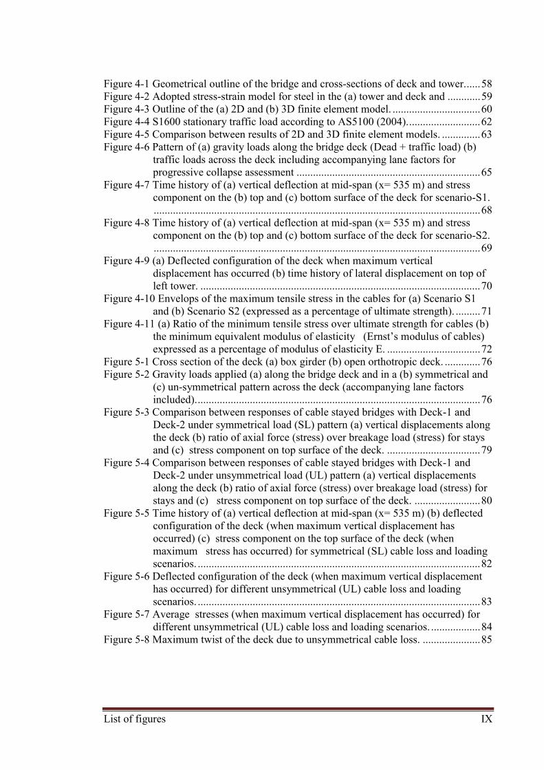
collapse may occur due to several reasons, such as wind (e.g. Tacoma narrow bridge),

earthquakes (e.g. Hanshin highway) traffic loads (e.g. I-35W Mississippi River Bridge)

and potentially some blast loadings. One of the most infamous bridge collapses is the

Tacoma Narrow Bridge in United States. This suspension bridge collapsed into the

Tacoma Narrow due to excessive vibration of the deck induced by the wind. The

collapse mechanism of this bridge is called "zipper-type collapse", in which the first

stay snapped due excessive wind-induced distortional vibration of the deck and

subsequently the entire girder peeled off from the stays and suspension cables. The

zipper-type collapse initiated by rupture of cable(s) also may occur in cable-stayed

bridges and accordingly guideline, such as PTI, recommends considering the probable

cable loss scenarios during design phase. Moreover, the possible extreme scenario

which can trigger the progressive collapse of a cable-stayed bridge should be studied.

Thus, there are three main objectives for this research, which are the effect of sudden

loss of critical cable(s), cable loss due to blast loadings and progressive collapse

triggered by the earthquake. A finite element (FE) model for a cable-stayed bridge

designed according to Australian standards is developed and analysed statically and

dynamically for this research purpose. It is noted that an existing bridge drawing in

Australia cannot be used due to a confidential reason. The bridge model has steel deck

which is supported by total of 120 stays. Total length of this bridge is 1070m with 600m

mid-span.

This thesis contains 8 chapters starting with the introduction as chapter 1.

In chapter 2, comprehensive literature review is presented regarding three main

objectives.

In chapter 3 to 5, results of the cable loss analyses are presented. In chapter 3, the

dynamic amplification factor (DAF) for sudden loss of cable and demand-to-capacity

ratio (DCR), which indicate the potential progressive collapse, in different structural

components including cables, towers and the deck are calculated corresponding with the

most critical cable. The 2D linear-elastic FE model with/without geometrical

Abstract IV

nonlinearity is used for this analysis. It is shown that DCR usually remains below one

(no material nonlinearity occurs) in the scenarios studied for the bridge under

investigation, however, DAF can take values larger than 2 which is higher than the

values recommended in several standards. Moreover, effects of location, duration and

number of cable(s) loss as well as effect of damping level on the progressive collapse

resistance of the bridge are studied and importance of each factor on the potential

progressive collapse response of the bridges investigated.

As it was shown in chapter 3, a 2D linear-elastic model is used commonly to determine

the loss of cable. However, there is a need to study the accuracy and reliability of

commonly-used linear elastic models compared with detailed nonlinear finite element

(FE) models, since cable loss scenarios are associated with material as well as

geometrical nonlinearities which may trigger progressive collapse of the entire bridge.

In chapter 4, 2D and 3D finite element models of a cable-stayed bridge with and

without considering material and geometrical nonlinearities are developed and analysed.

The progressive collapse response of the bridge subjected to two different cable loss

scenarios at global and local levels are investigated. It is shown that the linear elastic 2D

FE models can adequately predict the dynamic response (i.e. deflections and main

stresses within the deck, tower and cables) of the bridge subject to cable loss. Material

nonlinearities, which occurred at different locations, were found to be localized and did

not trigger progressive collapse of the entire bridge.

In chapter 5, using a detailed 3D model developed in the previous chapter, a parametric

study is undertaken and effect of cable loss scenarios (symmetric and un-symmetric)

and two different deck configurations, i.e. steel box girder and open orthotropic deck on

the progressive collapse response of the bridge at global and local level is investigated.

With regard to the results of FE analysis, it is concluded that deck configuration can

affect the potential progressive collapse response of cable-stayed bridges and the stress

levels in orthotropic open decks are higher than box girders. Material nonlinearities

occurred at different locations were found to be localized and therefore cannot trigger

progressive collapse of the entire bridge. Furthermore, effect of geometrical

nonlinearities within cables (partly reflected in Ernst’s modulus) is demonstrated to

have some effect on the progressive collapse response of the cable-stayed bridges and

accordingly should be considered.

Abstract V

In chapter 6, the blast loads are applied on the bridge model and determined the bridge

responses, since the blast load is one of the most concerned situations after 911 terrorist

attacks. The effect of blast loadings with different amount of explosive materials and

locations along the deck is investigated to determine the local deck damage

corresponding to the number of cable loss. Moreover, the results obtained from the

cable loss due to blast loadings are compared with simple cable loss scenarios (which

are shown in chapter 3 to 5). In addition, the potential of the progressive collapse

response of the bridge at global and local level is investigated. With regard to the results

of FE analysis, it is concluded that the maximum 3 cables would be lost by the large

amount of TNT equivalent material due to damage of the anchorage zone. Simple cable

loss analysis can capture the results of loss of cable due to blast loadings including with

local damages adequately. Short cables near the tower are affected by blast loadings,

while they are not sensitive for the loss of cables. Furthermore, loss of three cables with

damaged area did not lead progressive collapses.

Finally, in chapter 7, dynamic behaviour of cable-stayed bridges subjected to seismic

loadings is researched using 3D finite element models, because large earthquakes can

lead to significant damages or even fully collapse of the bridge structures. Effects of the

type (far- or near-field) and directions of seismic loadings are studied in several

scenarios on the potential progressive collapse response of the bridge at global and local

level. According to the case studies in this chapter, it is shown that near filed

earthquakes applied along the bridge affected to deck and cables significantly.

Moreover, the mechanism of bridge collapsed due to longitudinal excitation is analysed

by an explicit analysis, which showed the high plastic strain occurring around the pin

support created the permanent damage.

The summary and suggestions for this research are shown in final chapter 8.

Table of contents IV

Table of Contents Acknowledgement .......................................................................................... I List of Publications ...................................................................................... II Abstract ....................................................................................................... III Table of Contents ........................................................................................ IV List of Figures .......................................................................................... VIII List of Tables .............................................................................................. XII List of Symbols ........................................................................................ XIII Chapter 1 : Introduction ................................................................................ 1 1.1 Introduction ............................................................................................................... 1 1.2 Objectives .................................................................................................................. 3 1.3 Thesis Organization .................................................................................................. 6

Chapter 2 : Literature review ........................................................................ 8 2.1 Introduction ............................................................................................................... 8 2.2 Progressive collapse due to sudden loss of cable(s).................................................. 9 2.2.1 Background ......................................................................................................... 9 2.2.2 The effect of the critical cable loss ..................................................................... 9 2.2.3 Dynamic amplification factor (DAF) due to sudden loss of cable(s) .............. 10 2.3 Bridges subjected to blast loadings ......................................................................... 15 2.3.1 History of terrorist attacks ................................................................................. 15 2.3.2 Bridges subjected to terrorist attacks ................................................................ 15 2.3.3 Buildings subjected to blast loading ................................................................. 16 2.3.4 Bridges subjected to blast loadings ................................................................... 16 2.3.5 Cable-stayed bridges subjected to blast loadings .............................................. 17 2.4 Earthquake analysis ................................................................................................. 21 2.4.1 Background ....................................................................................................... 21 2.4.2 Cable-stayed bridge design in Japan ................................................................. 22 2.4.3 General seismic design for cable-stayed bridges .............................................. 23 2.4.4 Design criteria and standards ............................................................................ 26 2.5 Summary ................................................................................................................. 26

Table of contents V

Chapter 3 : Determining Critical Cable Loss Scenarios, DAF and DCR by 2D FE modelling ......................................................................................... 30 Summary of chapter ...................................................................................................... 30 3.1 Introduction ............................................................................................................. 30 3.2 Dynamic amplification factor (DAF) and demand-to-capacity ratio (DCR)…….. 3.3 Description of materials, geometry and loads ......................................................... 34 3.3.1 Material properties and geometry of the bridge ................................................ 34 3.3.2 Design loads ...................................................................................................... 36 3.3.3 Cable loss scenarios .......................................................................................... 36 3.3.4 Finite element model ......................................................................................... 37 3.3.5 Load combinations adopted for progressive collapse assessment .................... 37 3.3.6 Cable removal method and type of analysis ..................................................... 38 3.3.7 Discussion on the adequacy of the proposed 2D model ................................... 38 3.4 Parametric studies and discussion ........................................................................... 41 3.4.1 Time step over which the cable is removed (cable removal time step) ............ 41 3.4.2 Structural damping ............................................................................................ 46 3.4.3 Geometrical nonlinearities ................................................................................ 47 3.4.4 Cable removal scenarios ................................................................................... 47 3.5 Concluding remarks ................................................................................................ 54

Chapter 4 : Model verification - A Comparative Study of 2D and 3D FE Models of a Cable-Stayed Bridge Subjected to Sudden Loss of Cables .... 56 Summary of chapter ...................................................................................................... 56 4.1 Introduction ............................................................................................................. 56 4.2 Principal Assumptions ............................................................................................ 57 4.2.1 Geometry and material properties ..................................................................... 57 4.2.2 Modelling and analysis ..................................................................................... 60 4.2.3 Design Loads ..................................................................................................... 62 4.2.4 Calibration of 2D and 3D FE models ................................................................ 62 4.3 Cable Loss Scenarios .............................................................................................. 64 4.3.1 Cable removal method ...................................................................................... 64 4.3.2 Load combinations adopted for progressive collapse assessment .................... 64 4.3.3 Cable loss scenarios .......................................................................................... 65 4.3.4 Equivalent Modulus of Elasticity for Cables .................................................... 66 4.4 Results ..................................................................................................................... 67 4.4.1 Deck and Towers............................................................................................... 67

31

Table of contents VI

4.4.2 Cables ................................................................................................................ 70 4.5 Conclusions and Discussion .................................................................................... 72

Chapter 5 : Effect of loading pattern and deck configuration on the progressive collapse response of cable-stayed bridges ............................... 74 Summary of chapter ...................................................................................................... 74 5.1 Introduction ............................................................................................................. 74 5.2 Adopted assumptions .............................................................................................. 75 5.3 Cable loss scenarios ................................................................................................ 77 5.4 Analysis Results ...................................................................................................... 78 5.4.1 Healthy bridge (before loss of cables) .............................................................. 78 5.4.2 Deck and Tower ............................................................................................... 81 5.4.3 Cables ................................................................................................................ 86 5.4.4 Sensitivity Analysis ........................................................................................... 91 5.5 Conclusions and Discussion .................................................................................... 93

Chapter 6 : Cable-Stayed Bridges and Blast Loads .................................... 95 Summary of chapter ...................................................................................................... 95 6.1 Introduction ............................................................................................................. 95 6.2 Adopted assumptions .............................................................................................. 97 6.2.1 Geometry, material properties and design loads ............................................... 97 6.2.2 Modelling and analysis ..................................................................................... 97 6.2.3 Verification and calibration of LS-DYNA model (Explicit Solver) ............... 100 6.3 Blast load analysis and sudden loss of cable ......................................................... 101 6.3.1 Blast load analysis by explicit analysis (LS-DYNA) ...................................... 101 6.3.2 Load combinations adopted for blast and sudden loss of cable analyses ....... 103 6.3.3 Scenario considered for Blast load analysis .................................................... 103 6.3.4 Analysis of sudden cable loss using ALP approach and implicit solver

(ANSYS) ........................................................................................................ 106 6.4 Results and discussion .......................................................................................... 106 6.4.1 Results of blast analysis (LS-DYNA) ............................................................. 106 6.4.2 Comparative study between blast load and simple cable loss according to ALP

(blast around the pin support) ........................................................................ 109 6.4.3 Comparative study between blast load and simple cable loss according to ALP

(blast near tower and mid-span) ..................................................................... 116 6.5 Conclusions ........................................................................................................... 120

Table of contents VII

Chapter 7 : Dynamic Response of a Cable-Stayed Bridge Subjected to Seismic Loading ........................................................................................ 122 Summary of chapter .................................................................................................... 122 7.1 Introduction ........................................................................................................... 122 7.2 Adopted assumptions ............................................................................................ 123 7.3 Seismic analysis scenarios .................................................................................... 124 7.3.1 Seismic analysis method ................................................................................. 124 7.3.2 Scenario considered for Earthquake load analysis .......................................... 126 7.3.3 Earthquake acceleration data........................................................................... 126 7.3.4 Scenarios considered ....................................................................................... 127 7.4 Results and discussion .......................................................................................... 128 7.4.1 Results of implicit analysis (ANSYS model).................................................. 128 7.4.2 Progressive collapse analysis – Scenario K1 .................................................. 131 7.5 Effect of traffic load distribution on the seismic response .................................... 138 7.6 Sensitivity analysis ................................................................................................ 141 7.7 Preparing for experimental work .......................................................................... 144 7.7.1 Numerical model ............................................................................................. 144 7.7.2 Design for experimental model ....................................................................... 146 7.7.3 Pre-test ............................................................................................................ 148 7.7.4 Re-modelling ................................................................................................... 149 7.8 Concluding remarks .............................................................................................. 150

Chapter 8 : Conclusions ............................................................................ 151 8.1 Summary of each chapter ...................................................................................... 151 8.2 Overall Conclusions .............................................................................................. 155 8.3 Suggestion for further research ............................................................................. 155

References ................................................................................................. 157

List of figures VIII

List of Figures

Figure 1-1 Timber bridge damaged by floodwater (Pritchard, 2013) ............................... 1 Figure 1-2 Bridges damaged by tsunami (Unjoh, 2012) ................................................... 2 Figure 1-3 I-35W Mississippi River bridge collapse ........................................................ 2 Figure 1-4 Zipper-type collapse of the Tacoma Narrows Bridge (Starossek, 2011). ....... 3 Figure 2-1 A tied arch bridge ............................................................................................ 9 Figure 2-2 Bridge with under deck stay cable(s) ............................................................ 10 Figure 2-3 DAFs for cable-stayed bridge with sudden loss of cable .............................. 10 Figure 2-4 Bridge configurations - parameters considered in Mozos and Aparicio

(2010a) ............................................................................................................. 11 Figure 2-5 DAFs along the deck obtained from negative bending moment in all

scenarios with undamped and damped system ................................................ 12 Figure 2-6 A cable-stayed bridge model and cross sectional area of tower and deck used

in Hao and Tang, Tang and Hao (2010)........................................................... 16 Figure 2-7 Yokohama Bay Bridge .................................................................................. 19 Figure 2-8 The effect of tower shapes (Hayashikawa et al. (2000) ................................ 21 Figure 2-9 FEM model for multi-span cable stayed bridge (Okamoto and Nakamura,

2011) ................................................................................................................ 22 Figure 3-1 Different types of static analyses................................................................... 32 Figure 3-2 Adopted constitutive law for steel within deck and tower ............................ 34 Figure 3-3 Bridge elevation and principal dimensions. .................................................. 35 Figure 3-4 S1600 stationary traffic load according to AS5100.2 (2004). ....................... 36 Figure 3-5 Applied load cases. ........................................................................................ 37 Figure 3-6 Comparison of results obtained from 2D models developed in (a) ANSYS

and (b) MicroStran for the healthy bridge under LC-1. ................................ 39 Figure 3-7 Outline of the (a) 3D FE model and internal force and deflections predicted

by a (b) 2D linear-elastic model (c) 3D model with material & geometrical nonlinearity. .................................................................................................. 40

Figure 3-8 Time history of mid-span deflection predicted by 2D and 3D FE models for the bridge subjected to loss of cable no. 1 and LC-1. ................................... 40

Figure 3-9 (a) Load direction in the lost cable and (b) cable force versus time schemes adopted for dynamic removal of cables. ....................................................... 45

Figure 3-10 Time history of bending moment in scenario-1, case-3 at section C-C of the deck after removing cable no. 30 .................................................................. 45

Figure 3-11 Time history of bending moment in scenario-3 at section A-A of the deck obtained from dynamic analysis with different damping ratios. ................... 46

Figure 3-12 Time history of bending moment at the bottom of the left tower for different cable loss cases under scenario-1/LC-1 (only one cable is lost). ... 48

Figure 3-13 Time history of bending moment at the bottom of the left tower for different cable loss cases under scenario-1/LC-2 (only one cable is lost). ... 50

Figure 3-14 Time history of the bending moment at section A-A of the deck under scenario-2/LC-2 (two cables are lost). .......................................................... 52

Figure 3-15 DAF versus DCR values for scneaio-2 (LC-2, loss of cables no. 1 and 2). 53 Figure 3-16 DAF versus DCR values for scneaio-3 (LC-2, loss of cables no. 1, 2 & 3).

....................................................................................................................... 53

List of figures IX

Figure 4-1 Geometrical outline of the bridge and cross-sections of deck and tower. ..... 58 Figure 4-2 Adopted stress-strain model for steel in the (a) tower and deck and ............ 59 Figure 4-3 Outline of the (a) 2D and (b) 3D finite element model. ................................ 60 Figure 4-4 S1600 stationary traffic load according to AS5100 (2004). .......................... 62 Figure 4-5 Comparison between results of 2D and 3D finite element models. .............. 63 Figure 4-6 Pattern of (a) gravity loads along the bridge deck (Dead + traffic load) (b)

traffic loads across the deck including accompanying lane factors for progressive collapse assessment ................................................................... 65

Figure 4-7 Time history of (a) vertical deflection at mid-span (x= 535 m) and stress component on the (b) top and (c) bottom surface of the deck for scenario-S1. ....................................................................................................................... 68

Figure 4-8 Time history of (a) vertical deflection at mid-span (x= 535 m) and stress component on the (b) top and (c) bottom surface of the deck for scenario-S2. ....................................................................................................................... 69

Figure 4-9 (a) Deflected configuration of the deck when maximum vertical displacement has occurred (b) time history of lateral displacement on top of left tower. ...................................................................................................... 70

Figure 4-10 Envelops of the maximum tensile stress in the cables for (a) Scenario S1 and (b) Scenario S2 (expressed as a percentage of ultimate strength). ......... 71

Figure 4-11 (a) Ratio of the minimum tensile stress over ultimate strength for cables (b) the minimum equivalent modulus of elasticity (Ernst’s modulus of cables) expressed as a percentage of modulus of elasticity E. .................................. 72

Figure 5-1 Cross section of the deck (a) box girder (b) open orthotropic deck. ............. 76 Figure 5-2 Gravity loads applied (a) along the bridge deck and in a (b) symmetrical and

(c) un-symmetrical pattern across the deck (accompanying lane factors included). ....................................................................................................... 76

Figure 5-3 Comparison between responses of cable stayed bridges with Deck-1 and Deck-2 under symmetrical load (SL) pattern (a) vertical displacements along the deck (b) ratio of axial force (stress) over breakage load (stress) for stays and (c) stress component on top surface of the deck. .................................. 79

Figure 5-4 Comparison between responses of cable stayed bridges with Deck-1 and Deck-2 under unsymmetrical load (UL) pattern (a) vertical displacements along the deck (b) ratio of axial force (stress) over breakage load (stress) for stays and (c) stress component on top surface of the deck. ........................ 80

Figure 5-5 Time history of (a) vertical deflection at mid-span (x= 535 m) (b) deflected configuration of the deck (when maximum vertical displacement has occurred) (c) stress component on the top surface of the deck (when maximum stress has occurred) for symmetrical (SL) cable loss and loading scenarios. ....................................................................................................... 82

Figure 5-6 Deflected configuration of the deck (when maximum vertical displacement has occurred) for different unsymmetrical (UL) cable loss and loading scenarios. ....................................................................................................... 83

Figure 5-7 Average stresses (when maximum vertical displacement has occurred) for different unsymmetrical (UL) cable loss and loading scenarios. .................. 84

Figure 5-8 Maximum twist of the deck due to unsymmetrical cable loss. ..................... 85

List of figures X

Figure 5-9 Envelop of the (a) maximum tensile stress over ultimate strength (b) minimum tensile stress over ultimate strength and (c) the minimum equivalent modulus of elasticity (Ernst’s modulus of cables) expressed as a percentage of modulus of elasticity in the cables during symmetrical (SL) cable loss and loading scenarios. .................................................................. 87

Figure 5-10 Envelop of the maximum tensile stress in cables “a” (z=9.6) during unsymmetrical (UL) scenarios. ..................................................................... 88

Figure 5-11 Envelop of the maximum tensile stress in cables “b” (z=-9.6) during unsymmetrical (UL) scenarios. ..................................................................... 89

Figure 5-12 The minimum equivalent modulus of elasticity (Ernst’s modulus of cables) expressed as a ratio of modulus of elasticity during unsymmetrical (UL) scenarios. .............................................................................................. 90

Figure 5-13 Sensitivity of the deflected configuration of the deck (when maximum vertical displacement has occurred in scenario U4-UL) with respect to steel yield strength and elastic modulus . ........................................................... 91

Figure 5-14 Sensitivity of average stress component on top surface of the deck (when maximum vertical displacement has occurred in scenario U4-UL) with respect to steel yield strength and elastic modulus . .................................. 92

Figure 6-1 Outline of the 3D finite element models. ...................................................... 97 Figure 6-2 Comparison between results of 2D, implicit (ANSYS) and explicit (LS-

DYNA) 3D FE models (a) ratio of axial force (stress) over breakage load (stress) for stays (under service load) (b) stress component on top surface of the deck. ...................................................................................................... 100

Figure 6-3 Comparison of validation model with other references .............................. 102 Figure 6-4 Locations of the applied blast loadings. ...................................................... 104 Figure 6-5 Damages of the deck under blast loadings (blast occurred around pin-

support) ....................................................................................................... 107 Figure 6-6 Time history of stress (expressed as a percentage of breakage stress) for

cables No.1a and 1b (Scenario: 27t_7.5m). ................................................ 108 Figure 6-7 vertical displacements along the deck for scenarios with 1, 2 and 3 cable

losses. .......................................................................................................... 111 Figure 6-8 σxx stress component on top surface of the deck for scenarios with 1, 2 and 3

cable losses. ................................................................................................. 112 Figure 6-9 σxx stress component on bottom surface of the deck for scenarios with 1, 2

and 3 cable losses. ....................................................................................... 113 Figure 6-10 Envelop of the maximum tensile stress over breakage stress in the cables

“a” (z=9.6). .................................................................................................. 114 Figure 6-11 Envelop of the maximum tensile stress over breakage stress in the cables

“b” (z= - 9.6). .............................................................................................. 115 Figure 6-12 Maximum of (a) vertical deflection (b) σxx on top of the deck and (c) σxx

on bottom of the deck (loss of cable 30a). .................................................. 117 Figure 6-13 Maximum of (a) vertical deflection (b) σxx on top of the deck and (c) σxx

on bottom of the deck (loss of cable 15a). .................................................. 118 Figure 6-14 Cable stress ratio (loss of cables 30a/15a). ............................................... 119 Figure 7-1 The natural period and mode shapes for the first 6 natural modes of

vibration. ..................................................................................................... 125 Figure 7-2 (a) ground acceleration time history (b) acceleration response spectrum. .. 127 Figure 7-3 Vertical deflection along the deck (a) Scenario K2-K4 (b) Scenario E1-E4.

..................................................................................................................... 129

List of figures XI

Figure 7-4 σxx stress component on the (a) top and (b) bottom surface of the deck for scenario-K3 compared with healthy structure ............................................. 130

Figure 7-5 Envelop of the maximum tensile stress over ultimate strength in the cables (a) Scenarios K2-K4 and (b) Scenarios E1-E4. .......................................... 131

Figure 7-6 (a) has occurred along with stress components on the (b) top and (c) bottom surface of the deck for scenario-SH (only gravity loads) and scenario-K1.. ..................................................................................................................... 132

Figure 7-7 (a) σxx on bottom of the deck at 9.7 seconds and (b) time history of σxx at x= 7.5 m (stress exceeded the yield strength at 9.7 sec). ............................ 134

Figure 7-8 σxx and plastic strain around pin-support using ANSYS and LS DYNA .. 135 Figure 7-9 (a) Bridge configuration at 60 seconds (after earthquake) and (b) uplift of the

deck around the pin-support, Higashi-Kobe Bridge after 1995 Kobe Earthquake. .................................................................................................. 136

Figure 7-10 Time history of σeqv at the bottom of towers. .......................................... 136 Figure 7-11 (a) Envelop of the maximum tensile stress in the cables and (b) time

histories of tensile stress in cables No.1 and No. 48. .................................. 137 Figure 7-12 Traffic load distribution............................................................................. 138 Figure 7-13 σxx on bottom of the deck around 10 seconds into the K5 earthquake

scenario (first element reached the plastic strain). ...................................... 139 Figure 7-14 Envelop of (a) vertical displacement and (b) σxx on the bottom surface of

the deck at 60 seconds into the K5 earthquake scenario. ............................ 140 Figure 7-15 Envelop of the maximum tensile stress in the cables. ............................... 141 Figure 7-16 σxx on the bottom of deck at 9.7 seconds into the K5 earthquake scenario.

..................................................................................................................... 142 Figure 7-17 (a) Deflected configuration of the deck and (b) σxx on the bottom surface

of the deck at 60 seconds into the K5 earthquake scenario. ........................ 142 Figure 7-18 Envelop of the maximum tensile stress in the cables ................................ 143 Figure 7-19 Configuration for numerical model ........................................................... 145 Figure 7-20 Experimental bridge model (dimensions in mm) ...................................... 147 Figure 7-21 End support system for experimental prototype........................................ 148 Figure 7-22 Devised mechanism for post-tensioning the cables. ................................. 148 Figure 7-23 (a) Prototype on the shake table, (b) LVDT and (c) accelerometer .......... 149

List of Tables XII

List of Tables Table 2-1 Earthquake intensity ....................................................................................... 20 Table 3-1 Material and geometrical properties of the deck, towers and cables. ............. 33 Table 3-2 Scenarios considered. ..................................................................................... 36 Table 3-3 Maximum DCR and corresponding DAF values for scenario-1/LC-1 in which

one cable is lost (Gravity load case 1- critical damping ratio is taken as 0.5%) ............................................................................................................. 42

Table 3-4 Maximum DCR and corresponding DAF values for scenario-2/LC-2 in which two cables are lost (Gravity load case 2- critical damping ratio is taken as 0.5%). ............................................................................................................ 43

Table 3-5 Maximum DCR and corresponding DAF values for scenario-3/LC-2 in which three cables are lost (Gravity load case 2). ................................................... 44

Table 3-6 Maximum DCR and corresponding DAF values in towers, deck and cables under scenario-1/LC-1 (Gravity load case 1 – critical damping ratio is taken as 0.5%). ........................................................................................................ 49

Table 3-7 Maximum DCR and corresponding DAF values for scenario-1/LC-2 in which one cable is lost (Gravity load case 2 - critical damping ratio is taken as 0.5%). ........................................................................................................ 51

Table 3-8 Maximum DCR and corresponding DAF values in towers, deck and cables under scenario-1/LC-2 (Gravity load case 2 - critical damping ratio is taken as 0.5%). ........................................................................................................ 51

Table 4-1 Material and geometrical properties of the deck, towers and cables. ............. 59 Table 4-2 The periods of the first five in-plane global natural modes of vibration. ....... 64 Table 4-3 Cable loss scenarios considered in this chapter. ............................................. 66 Table 4-4 Material and geometrical properties of the deck, towers and cables. ............. 67 Table 5-1 Cable loss scenarios and loading patterns considered in this study................ 78 Table 5-2 Summary of the maximum twist (θmax), maximum stresses within the deck,

maximum drift on top and maximum equivalent stresses on the bottom of the right tower obtained from unsymmetrical load pattern and cable loss scenarios ........................................................................................................ 85

Table 6-1 Scenarios considered for blast load analysis (using LS-DYNA software). .. 105 Table 6-2 Scenarios considered - equivalent cable loss analysis (simple cable loss

analysis) -implicit analysis by ANSYS ....................................................... 106 Table 6-3 Summary of the cable losses and damaged areas obtained from blast load

analysis. ....................................................................................................... 108 Table 6-4 Summary of maximum deflection, stresses for deck and tower obtained from

explicit analysis (blast loading analysis) and implicit analysis (loss of cable analysis) ....................................................................................................... 110

Table 7-1 The natural frequency and period of the first fifteen modes of vibration. .... 124 Table 7-2 Scenarios considered for applying seismic action. ....................................... 128 Table 7-3 Summary of the maximum vertical deflections, drift on top of right tower and

stresses within the deck obtained from implicit 3D ANSYS FE models. ... 129 Table 7-4 Summary of sensitivity analysis results. ....................................................... 144 Table 7-5 Deck properties. ............................................................................................ 146

List of Symbols XIII

List of Symbols A Cross-sectional area b Width of the deck CLDF Cable loss dynamic forces DC Dead load of structural components and non-structural attachments DW Dead load of wearing surfaces and utilities E Modulus of elasticity E Equivalent modulus of elasticity Esh Hardening modulus of steel EV Extreme event load I Moment of inertia of the section IM Vehicular dynamic load allowance taken l Horizontal span LL Full vehicular live load placed in actual stripped lanes M Bending moment My Yield moment N Axial force Ny Yield Force R Distance between contact surface and the denote centre t Thickness of the steel plate W Equivalent TNT amount y Distance from the neutral axis moment of inertia of the section Z Scaled distance (in m/kg1/3),

i-PT Initial post-tensioning strain in cables Density Existing stress from dynamic analysis

u Ultimate stress y Yield stress

λey Yield limit slenderness ratio

Chapter 1 Page 1

: Introduction Chapter 1

1.1 Introduction Bridge structures are often subjected to severe conditions, such as wild weather,

earthquakes, impact of traffic accidents and even explosions. As a result of such

extreme external loads, bridge structures could suffer loss of some of their critical

structural members (e.g. cables or piers) and subsequent collapse may occur, since a

progressive collapse is typically triggered by a sudden loss of one or more critical

structural components.

In 2011, the state of Queensland in Australia experienced severe floods. A significant

economic damage (a total of 4.5 billion Australian dollars) was sustained as a result of

roadway and railway damages and closure, including bridge structures (Lee et al., 2013,

Roads, 2012, Pritchard, 2013). In Japan, a magnitude 9.0 earthquake followed by large

Tsunami created enormous damage to a large area of a coastal region. The estimated

cost of damage was in tens of billions of US dollar (Nakanishi et al., 2013). About 30 of

Japanese railway bridges, viaducts (101 girders lost) and hundreds of kilometres of

highway were damaged (Kawashima et al., 2011; Koseki et al., 2012, Unjoh, 2012).

Figure 1-1 Timber bridge damaged by floodwaters (Pritchard, 2013).

Chapter 1 Page 2

Figure 1-2 Bridges damaged by tsunami (Unjoh, 2012).

Figure 1-3 I-35W Mississippi River bridge collapse.

Some of the bridges collapsed due to various loading conditions are shown in Figures 1-

1 to 1-3. During the evening rush hour on 1st of August 2007, I-35W Mississippi

River Bridge suddenly crashed into the river. 13 people were killed and many people

suffered serious injuries. Design failure was identified as one of the most significant

causes of this collapse, although heavy traffic load was a contributing factor as well

(Hao, 2010). Moreover, after the 911 terrorist attacks, structural collapses due to

malicious actions have become a critical factor in bridge design. According to a

Canadian transportation report, about 199 bridges were attacked or considered to be

attacked by terrorists between 2002 and 2008 (Canada, 2009). Also, Jenkins and

Gersten (2001) reported in the FTA report that about 58% of terrorist attacks targeted

the transportation sector including bridge structures.

Collapses or critical damages to bridges can significantly affect the economy as well as

human lives, thus bridges should be designed to withstand these severe conditions.

Chapter 1 Page 3

1.2 Objectives In this research, cable-stayed bridges are the main subject, since Road and Maritime

Service (RMS) of NSW government in Australia is interested in dynamic behaviour of

this type of bridge under severe loading conditions. Considering the high cost of

experimental work for testing large scale bridges, the best and perhaps the only

available option for such studies would be advanced numerical models which can

properly capture local and global behaviour of the structure including material and

geometrical nonlinearities. In this research, ANSYS and LS-DYNA software are

employed to conduct finite element (FE) analyses and simulate the behaviour of cable

stayed bridges subjected to extreme loading scenarios such as cable loss, blast and

earthquake. The developed FE models can take account of material as well as

geometrical non-linearity. Also, the effect of inertia and dynamic loads are considered

in the FE models.

Cable-stayed bridges as well as suspension bridges can be exposed to severe loading

conditions and might be damaged as a result. One of the most notable bridge collapses

has been the spectacular collapse of the Tacoma Narrows Bridge in the United States

due to aerodynamic instability caused by wind loads. The bridge’s main span collapsed

into the Tacoma Narrow on 7th November 1940, four months after it was opened. The

main reason for the collapse of Tacoma Narrows Bridge was wind-induced resonance

and the ratio between the span and the deck depth as well as very low torsional stiffness

of the deck (Kwon and Qian, 2012, Miyachi et al., 2012). In Tacoma bridge case, the

first stay snapped by excessive wind-induced distortion of the bridge deck, the entire

girder peeled off from the stays and suspension cable(s) as seen in Figure 1-4. Such

cable loss scenarios can/may lead to high impulsive dynamic loads in the structure that

can potentially trigger a “zipper-type” progressive collapse of the entire bridge

(Starossek, 2011).

Accordingly, in cable-stayed bridges, the likelihood of occurrence of progressive

collapse triggered by cable loss scenarios must be thoroughly investigated. PTI (2007)

recommends considering the probable cable loss scenarios during the design phase.

Static analysis and application of a Dynamic Amplification Factor (DAF) of 2 is

recommended to determine the effect of loss of cable(s). However, some researchers

Chapter 1 Page 4

have questioned the validity of static analyses in conjunction with a single value DAF

(Mozos and Aparicio, 2010a, Mozos and Aparicio, 2010b, Starossek, 2011).

The initial objectives of this thesis are,

1) accurately determine the DAF corresponding to the location/number of cable

loss(s) as well as the effect of damping ratio

2) determine the relation between DAF and potential progressive collapse which is

identified by the Demand-Capacity Ratio (DCR)

3) in the context of alternate load path method (ALP), identify the most critical

cable(s) which their loss can potentially trigger the progressive collapse of the

entire bridge

4) evaluate the influence of loading patterns (i.e. unsymmetrical and symmetrical)

in conjunction with different cable loss scenarios on the potential progressive

collapse response of the bridge

Figure 1-4 Zipper-type collapse of the Tacoma Narrows Bridge (Starossek, 2011).

For cable-stayed bridges, the cables and their anchorage zones have relatively small

cross sectional areas and are exposed to severe loading conditions (e.g. corrosion,

impact of vehicles and blast). These extreme loads can cause damage to the anchorage

zones as a result of high stress concentration, and can lead to loss of cables (Yang et al.,

2011, Tang and Hao, 2010, Hao and Tang, 2010, Tang, 2009, Åkesson, 2008, Hao,

Chapter 1 Page 5

2010, Starossek, 2011, Kiger et al., 2010, Mitchell et al., 2006). In this thesis, malicious

actions in the form of blast loadings are chosen since the blast loadings analysis is one

of the most important topics for iconic structures like bridges after 911 terrorist attacks.

With regard to the research reported in the literature that specifically relates to bridges

subjected to blast loadings, in the second part of this thesis finite element models of a

cable stayed bridge are developed and analysed using LS-DYNA software. Also, the

explosive charge and process of air blast propagation are directly modelled in the LS-

DYNA software. The main focus of this second part is to

5) identify the type and extent of the damages caused by air blast in the vicinity of

anchorage zone of cable

6) determine the number of lost cables following blast scenarios in which the size

and location of explosives vary

7) evaluate the dynamic response of the cable-stayed bridges following loss of

cable(s) caused by direct blast loadings.

8) evaluate the accuracy of alternate load path (ALP) for capturing the behaviour of

cable stayed bridges subjected to blast loading

Finally, the detailed continuum-based finite element models developed in ANSYS and

LS-DYNA software are employed to capture the dynamic behaviour of a cable-stayed

bridge under earthquake loadings and

9) determine the most critical direction and type of seismic loadings

10) identify the critical structural components that suffer the most damage under the

earthquake loadings

11) identify the damage mechanism and mode of failure in cable stayed bridges

subject to seismic action

Initially the ANZAC bridge was supposed to be considered in this research project,

however, due to security and confidentiality reasons the analysis of an existing bridge in

Australia was ruled out by RMS as the main sponsor of this research project.

Accordingly, for this project a cable stayed bridge was analysed and designed according

to minimum requirements of Australian standards.

Chapter 1 Page 6

1.3 Thesis Organization The thesis consists of 8 chapters as follows:

1) Chapter 1 presents a brief background and introduction of the thesis and the

main objectives of the research.

2) Chapter 2 reviews the relevant literature on the three main topics including cable

loss analysis and the magnitude of dynamic amplification factor (DAF) for

bridges subjected to blast loadings and the dynamic behaviour of bridges under

seismic loadings.

3) Chapter 3 aims to determine the DAFs associated with different sudden cable

loss scenarios. The effects of location, duration and number of lost cable as well

as the effect of damping level on the progressive collapse response of the bridge

are studied. The importance of each factor on the potential progressive collapse

response of the bridges is identified and the demand-to-capacity ratio (DCR) in

cables, towers and the deck are calculated for most critical cable loss scenarios.

A 2D linear-elastic FE model with and without geometrical nonlinearity is used

for this analysis.

4) In Chapter 4 a non-linear 3D continuum-based finite element model of the

bridge is developed with full details and analysed. The accuracy of the linear

elastic 2D model and DCRs calculated in Chapter 3 in comparison with the

detailed nonlinear 3D FE model is verified in this chapter.

5) Chapter 5 investigates the effects of different symmetric and unsymmetric

loading patterns and cable loss scenarios. The unsymmetric loading patterns and

cable loss scenarios can induce torsional mode of vibration in the deck and

subsequently trigger the progressive collapse of the entire bridge. Also, the

effect of deck configuration (i.e. steel box girder and an open orthotropic deck)

on the progressive collapse response of the cable stayed bridge is investigated in

conjunction with loading and cable loss patterns.

6) In Chapter 6, dynamic repose of the bridge subjected to blast loading is

investigated. The explosive and air blast are directly modelled to determine the

number of lost cables and extent of the damage around the anchorage zone

Chapter 1 Page 7

during such loading scenarios. Different amounts of TNT equivalent explosives

at different locations are considered in the analyses. In addition, the global

response due to the loss of cable caused by blast loading is compared with the

simple cable loss analysis (obtained in Chapters 3 and 4) in order to verify the

accuracy of ALP method based on simple cable loss scenarios.

7) Chapter 7 focuses on the dynamic response of the cable-stayed bridge subjected

to two different types of earthquake accelerations (i.e. horizontal and vertical).

Also, the seismic accelerations are applied in four different directions (different

angle of attack with respect to longitudinal axis of the bridge) to determine the

most critical type of earthquake as well as the critical angle of attack. Moreover,

using LS-DYNA FE model, the damage mechanism and failure mode of the

bridge is determined under the most critical earthquake loadings.

8) Chapter 8 concludes the research work and highlights some recommendations

for future studies regarding behaviour of cable stayed bridges subjected to

extreme loading scenarios.

Chapter 2 Page 8

: Literature review Chapter 2

2.1 Introduction In cable-stayed bridges, damage or failure of primary structural components such as

tower, piers or cables, caused by extreme loadings can lead to the collapse of the entire

bridge. For this type of bridge, zipper-type collapse (defined as a horizontal progressive

collapse) is one of the most concerning failure modes that can be caused by the sudden

loss of cables. Analysis of sudden loss of cables in cable stayed and suspension bridges

is extremely critical and it has drawn the attention of researchers in recent years and it is

one of the main objectives of this research. This section presents a review of past

research on the effects of sudden loss of cable, the collapse mechanism of the bridge

and different analysis methods (i.e. dynamic analysis and static analysis with dynamic

amplification factor) available for progressive collapse assessment of cable bridges.

Progressive collapse initiated by the loss of critical structural components occurs over a

short period of time due to high strain rate loadings such as blast or impact. Since the

collapse of Ronan Point apartment building in 1968, progressive collapse has been an

important issue in structural design and a significant amount of research has been

conducted on progressive collapse response of building structures subjected to extreme

loading scenarios (Vlassis et al., 2009, Nethercot et al., 2007, Choi and Kim, 2011,

Lange et al., 2012, Stoddart et al., 2013). Apart from building structures, the dynamic

behaviour of the bridge structures subject to extreme loading scenarios (e.g. blast

loadings) and critical member loss are currently of high interest to structural engineers

and researchers. Accordingly, a comprehensive literature review regarding the effect of

the explosions on bridge structures, particularly cable-stayed bridges, is presented in

this chapter.

Seismic actions have caused severe damage, including progressive collapse of the

bridge structures in the past, and are considered as one of the most important extreme

cases in bridge design. Accordingly, a comprehensive literature review on earthquake

analysis of bridge structures is also reported in this chapter.

Chapter 2 Page 9

2.2 Progressive collapse due to sudden loss of cable(s)

2.2.1 Background

Stays of cable-stayed bridges are critical structural elements which are subjected to

corrosion, abrasion, wind, vehicle impact and malicious actions and these extreme

loading scenarios may lead to severe damage and loss of cable(s) (Åkesson, 2008,

Walther, 1999, Yang et al., 2011, Ghali and Krishnadev, 2006, Jo et al., 2002). Such

cable loss scenarios can/may lead to high impulsive dynamic loads on the structure that

can potentially trigger a “zipper-type” progressive collapse of the entire bridge, like

Tacoma Narrows Bridge, although it was a suspension bridge (Starossek, 2011, Plaut,

2008). Accordingly, cable-stayed bridges should be designed for potential cable loss

scenarios as recommended by the guidelines such as PTI (2007). This standard requires

that the cable-stayed bridges should be able to withstand the loss of any cable without

the occurrence of structural instability or progressive collapse.

2.2.2 The effect of the critical cable loss

Kao and Kou (2010) analysed a symmetrical, fan-shaped cable-stayed bridge under

sudden breakage of cable. They determined the dynamic response of the entire bridge

including bending moment along the deck, the deflection along the deck and at top of

the tower, deviation of axial forces in each cable and stresses in the girders and tower.

Also, the ultimate load-bearing capacity of different structural components were

determined and compared with maximum tractions induced in each component to

determine whether any failure occurs. The cable connected to the pin supports was

identified as the most critical cable which its loss leads to a high increase of sagging

deformation of the deck and tower stress. In addition, the cable connected to the mid-

span was found out to be the second most critical cable which its loss can lead to a

dramatic increase in the girder stresses.

Wolff and Starossek (2008) studied the collapse behaviour of a 3D cable-stayed bridge

model and found out that the initial failure (loss) of the three cables around the pylon

can trigger a zipper-type collapse associated with a large vertical deformation within the

bridge deck. In the failure mechanism identified by Wolff and Starossek (2008), the loss

of cables lead to high stress concentration in the cables adjacent to the lost ones and

Chapter 2 Page 10

subsequently these adjacent cables snap. Also, it was concluded that the extent of

collapse triggered by the cable loss strongly depends on the location of the lost cable.

2.2.3 Dynamic amplification factor (DAF) due to sudden loss of cable(s)

The progressive collapse of the structures triggered by extreme events typically has a

dynamic nature. However, in practice and for progressive collapse assessment of the

structures, a static analysis is considered to be adequate, providing a proper dynamic

amplification factor (DAF) is applied on the static analysis results (Kokot et al., 2012).

The value of DAF adopted by different standards and guidelines varies between 1.5 and

2 (DoD, 2005, GSA, 2003, PTI, 2007). For example, the Stonecutters Bridge in Hong

Kong was designed using a DAF of 1.5 (ARUP, 2010, Hussain et al., 2010).

Apart from the magnitude of DAF, the definition of DAF in the context of cable

structures is slightly different than the DAF specified in the building codes. DAF for a

cable-stayed bridge with cable loss is generally specified as follows (Zoli and

Woodward, 2005):

DAF 2-1

where α is value of response obtained from the current state prior to cable loss (static

analysis without cable loss), β is the response obtained from a static analysis after the

cables are lost and γ is the value of response captured by a dynamic cable loss analysis.

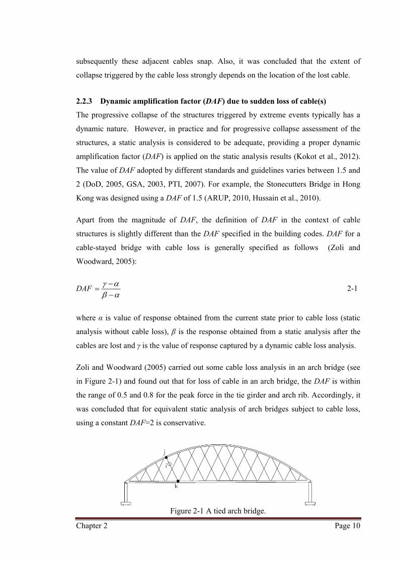
Zoli and Woodward (2005) carried out some cable loss analysis in an arch bridge (see

in Figure 2-1) and found out that for loss of cable in an arch bridge, the DAF is within

the range of 0.5 and 0.8 for the peak force in the tie girder and arch rib. Accordingly, it

was concluded that for equivalent static analysis of arch bridges subject to cable loss,

using a constant DAF=2 is conservative.

Figure 2-1 A tied arch bridge.

Chapter 2 Page 11

In a different study, Ruiz-Teran and Aparicio (2007) have argued that the application of

DAF=2 (obtained for a system with single degree of freedom) for cable-stayed bridges

with multi-degrees-of-freedom is not always conservative. Accordingly, Ruiz-Teran and

Aparicio (2007) determined the DAF values for the case of sudden loss of cable(s) in a

cable-stayed bridge. Ruiz-Teran and Aparicio (2007) found out that a load due to

sudden cable loss causes the structure to deform and to oscillate around the new

deformed position, thus DAFs should be determined considering the dynamic response

of the real structure with multiple degrees of freedom. Also, it was concluded that DAF

for each parameter of interest (i.e. deflection, bending moment and shear force) should

be determined separately. The value of DAFs for bending moments along a bridge with

under-deck stay cables is shown in Figure 2-2. It is observed that at several locations

along the deck, DAF has taken values larger than 2. For example, the DAF is about 4 at

a section 4 m away from the support at the far left side of the bridge deck.

Wolff and Starossek calculated the DAFs for bending moments along the bridge deck of

a conventional cable-stayed bridge as shown in Figure 2-3 (Wolff and Starossek, 2008,

Wolff and Starossek, 2009, Wolff and Starossek, 2010).

Figure 2-2 Bridge with under deck stay cable (Ruiz-Teran and Aparicio, 2007).

Chapter 2 Page 12

With regard to Figure 2-3, it is observable that DAFs exceed 2 at several locations along

the deck. They found that applying a single DAF for different structural components in

a cable-stayed structure cannot adequately capture the dynamic effects, because the

value of DAF for each structural component depends on the location of the lost cable as

well as type of the state variable (i.e. deflection, shear force, bending moment) under

consideration.

(a) Bridge configuration

(b) DAFs for bending moment along the deck

Figure 2-3 DAFs for cable-stayed bridge with sudden loss of cable (Wolff and

Starossek, 2010).

Moreover, a parametric study on the dynamic response of a series of hypothetical cable

stayed bridges subjected to sudden failure of a stay have been conducted to determine

the importance of the accidental ultimate state of failure of a cable in design and also

investigate the adequacy of a simplified equivalent static analysis in which a DAF=2 is

adopted (Mozos and Aparicio, 2010a, Mozos and Aparicio, 2010b).

Mozos and Aparicio (2010a&b) studied the characteristics of different bridge models

and the factors that can influence the dynamic collapse response of the cable-stayed

Chapter 2 Page 13

bridges subjected to loss of one stay. The parameters considered in Mozos and

Aparicio (2010a&b) includes two different damping ratios (i.e. ξ=0% & 2%), two

different types of cable configuration (i.e. fan and harp patterns), three different deck

dimensions and two types of pylons (I and H shape) as shown in Figure 2-4.

(a) Bridge configuration – longitudinal layout of the fan and harp pattern

(b) Dimensions of the deck (c) Pylon design

Figure 2-4 Bridge configurations - parameters considered in Mozos and Aparicio

(2010a).

Chapter 2 Page 14

To determine the DAF, finite element models were developed and analysed using both

equivalent static approach and dynamic time integration (Newmark’s time marching

scheme). The value of DAFs for negative bending moment during a cable loss scenario

for different bridge configurations and damping ratios are shown in Figure 2-5. It is

observed that the DAF obtained for negative bending moment exceeds the value of 2 as

predicted in previous studies by Ruiz-Teran and Aparicio (2007). The maximum DAF

values are 8.0 and 5.6 in the un-damped and damped systems, respectively, and the

average values are 3.35 and 2.52, respectively. Also it is seen that the layout of the stays

(i.e. fan (F) or harp (H) types) as well as the dimension and configuration of the deck

can significantly influence the DAF values.

Moreover, a small-scale test was conducted to evaluate the DAFs for the structures

subjected to sudden loss of support and it was observed that the experimental DAFs are

typically larger than the DAF=2 adopted by design standards and guidelines (Mozos

and Aparicio, 2011, Tsai and You, 2012).

With regard to the existing literature on the DAF values, it can be concluded that a

single value DAF cannot adequately take account of dynamic effects in the equivalent

static analysis. Also, a DAF=2 is not always conservative according to the existing

research in the literature.

Figure 2-5 DAFs along the deck obtained from negative bending moment in all

scenarios with undamped and damped system.

Chapter 2 Page 15

2.3 Bridges subjected to blast loadings

2.3.1 History of terrorist attacks

Due to the increase in terrorist attacks in recent years, blast loads have been recognized

as one of the extreme events that must be considered in the design of important

structures.

Well-known examples of terrorist attacks are the Alfred P. Murrah Federal Building in

Oklahoma City (1995) and the World Trade Center in New York City (2001). The most

well-known terrorist event for the Australians is the ‘Bali bombing’ on 12th October

2002 (Southwick et al., 2002, Mendis and Ngo, 2003). It occurred in a popular

nightclub in Bali. A total of 88 Australians were killed. The most recent terrorist attack

related to Australia was in Jakarta in 2009. Three Australian business men were killed

in this attack (Smith, 2013). Moreover, London terrorist attacks on 7 July 2005 were

unforgettable events in UK (Emergency Management Australia, 2007). After the

London terrorist attacks, the Australian government held a workshop to prepare for such

terrifying events (Emergency Management Australia, 2007).

2.3.2 Bridges subjected to terrorist attacks

Terrorists have targeted iconic structures such as the World Trade Center, the London

metro, famous night clubs and luxury hotels. Accordingly, iconic bridges are not

immune from such terrorist attacks.

According to a Canadian transportation report, about 199 bridges were attacked or

considered to be attacked by terrorists between 2002 and 2008 (Canada, 2009). Also,

Jenkins and Gersten (2001) reported in an FTA report that about 58% of terrorist attacks

targeted the transportation sector including bridge structures.

Mahoney (2007) analysed typical highway bridges under blast loads, while Bensi et al.

(2005) investigated the risk of terrorist attacks on a cable-stayed bridge and both

authors calculated the economic consequences of such attacks that would be quite

significant and in some cases the cost would be over $100 million. Although it is a rare

case, if a bridge is subjected to a full scale terrorist attack, the structure might fully

collapse. Even some minor damage may require the bridge to be closed for repairs, that

may have significant economic implications.

Chapter 2 Page 16

2.3.3 Buildings subjected to blast loading

Responses of the structures or the structural components subjected to blast loadings

have been studied experimentally and numerically (Jacinto et al., 2001, Li and Meng,

2002, Lawver et al., 2003, Lam et al., 2004, Ngo and Mendis, 2005, Ngo et al., 2005b,

Gram et al., 2006). Also, the characteristics of the materials (such as different strength

concrete or steel) subjected to impact loads were determined (Ngo et al., 2005a, Zhang

et al., 2005, Ngo et al., 2007b, Zhang et al., 2007, Wright and French, 2008).

After the 911 World Trade Center terrorist attacks, it was recognised that damage by

initial blast loads could lead to the progressive collapse of the entire building.

Ngo et al. (2007a) reviewed the blast load effects on the structures. They analysed the

local damage of columns and the progressive collapse of an entire building which is a

52 storey building modified from a typical tall building in Australia (AS/NZS1170.2,

2002). It was found that two columns, slabs and beams above the lost columns were

destroyed by the blast loadings directly. Also, it was found that if more than two floors

are destroyed by blast, the progressive collapse of the entire building may be triggered.

Also, Kwasniewski (2010) studied a potential progressive collapse of a 8-storey

building subjected to loss of a column at the first floor by using the LS-DYNA

software. They analysed three different locations of column loss, and concluded that

there was a low possibility for a progressive collapse of this particular building.

2.3.4 Bridges subjected to blast loadings

Damage of individual bridge components (such as piers and towers, cable and deck) due

to blast loadings has been studied for several types of bridge structures.

Piers and towers

A 2-span 2-lane bridge with typical type III AASHTO girders was developed and

analysed under blast loads by using STAAD.Pro and AT Blast software (Anwarul Islam

and Yazdani, 2008). This bridge model was assumed to be made of concrete

(compressive strength range between 31 MPa to 45 MPa) and subjected to the

equivalent TNT value of 226.8kg (regular truck). It was concluded that this type of

bridge will fail when the blast load is applied above or underneath the deck. Therefore,

Chapter 2 Page 17

Anwarul Islam and Yazdani (2008) recommended that design for blast resistance and

retrofit techniques for bridges should be developed and adopted in design guidelines.

Fujikura et al. (2008) proposed a new concrete-filled steel tube column system which

was investigated experimentally under blast loading. This system was shown to be

effective for blast resistance since breaching and spalling of concrete are effectively

prevented from occurring in this column.

Bridge Deck

Winget et al. (2005) reported a simulation of a concrete beam bridge subjected to blast

loads. They considered various locations of detonation to gain a better perspective of

the bridge performance against explosion. They concluded that the bridge used in their

research showed high vulnerability to failure under the impact of a conventional

vehicular bomb. They also argued that the response of bridges against blast load

depends significantly on the bridge geometry.

Design criteria for post-tensioned box girder bridges subjected to blast loadings were

presented by Kiger et al. (2010). The design criterion was derived with respect to the

numerical results captured by LS-DYNA software. In their report, the main design

criteria predict the relation between the equivalent explosive material size and the type

of damage (e.g. no damage, spall and breach of concrete).

2.3.5 Cable-stayed bridges subjected to blast loadings

The damage criteria and dynamic response of the cable-stayed bridges subjected to blast

loadings are discussed in this section. The results of the research in this field is limited

to the full scale cable-stayed bridges modelled and analysed by different researchers

(Hao and Tang, 2010; Tang and Hao, 2010) such as the one shown in Figure 2-6.

Bridge Pier and towers

A cable-stayed bridge with two different types of pylon (i.e. hollow steel box and

concrete-filled composite pylon) subject oblast load was studied by Son and Lee (2011).

Car bomb detonation was the scenario considered and simulated by dynamic-nonlinear

analysis using a combined Lagrangian and Eulerian model. The explicit numerical

software used in this study was MD Nastran SOL 700 (2011) to simulate the spatial and

time variation of the blast load and shock wave.

Chapter 2 Page 18

(a) Whole Bridge

Figure 2-6 A cable-stayed bridge model and cross sectional area of tower and deck used

in Hao and Tang, Tang and Hao (2010).

(b) Pier and Tower cross section

(c) Deck cross section

Chapter 2 Page 19

From the results of numerical model, Son and Lee (2011) concluded that a concrete-

filled pylon could survive while the hollow steel box section would collapse due to a

significant P-Δ effect under the same amount of explosive materials.

The concrete pier shown in Figure 2-6(b) was subjected to 1,000kg TNT explosion at

0.5m distance to determine the local damage cause by the air blast (Hao and Tang,

2010, Tang and Hao, 2010). According to Tang and Hao (2010), the surface of the pier

facing the blast load showed significant damage. The web and back of the pier wall had

more significant damage than the front wall. Accordingly, the damage in the pier led to

significant bridge deck deformation, for instance the maximum vertical downward

deflection at mid-span was 11.52 m. Moreover, a part of the deck connected to this pier

fell down though the progressive collapse of the entire bridge was concluded to be

unlikely.

The tower, shown in Figure 2-6b, was also studied under the same amount of TNT (Hao

and Tang, 2010; Tang and Hao, 2010). However, due to the large wall thickness (2m)

and the absence of web segments inside the tower, the local damage of the tower was

only seen on the front surface (blast applied) of the tower. Furthermore, this local

damage on the front surface did not trigger a progressive collapse. However, when the

amount of explosives was increased to 10,000 kg of TNT (applied at 6.5m distance

from the tower), the entire bridge did collapse due to shear failure and flexural failure

on the side and rear walls of the tower. According to the parametric study conducted, if

complete damage of the entire tower cross section does not occur, progressive collapse

of the bridge structure is unlikely. Also, it was concluded that the progressive collapse

of the entire bridge can be prevented, provided a minimum 12 m stand-off distance is

required.

Deck

Deng and Jin (2009) analysed the effect of blast loads numerically. The actual bridge,

named Minpu II Bridge in Shanghai was used as the benchmark bridge. The blast

charge assumed was an 800 kg TNT placed on top of the bridge deck. The ANSYS

AUTODYN computer program (2007) was used for blast load simulation. It was shown

that the stress concentration due to blast load is limited to the blast region and cracks are

distributed in small areas.

Chapter 2 Page 20

In Hao and Tang’s (2010) study, the bridge had two different types of deck, the back

span is a concrete deck and the mid span is a steel composite deck (see Figure 2-6(c)).

Due to the differences in material properties, the steel deck showed less damage than

the concrete deck. The damaged area of concrete deck is 30 m in length and 20 m in

width whereas the damaged zone in the steel deck is 11.5 m wide and 10 m long.

Son and Astaneh-Asl (2011) focused on the response and failure mode of a bridge deck

subjected to blast loadings. A typical orthotropic deck for cable-stayed bridges was

created using nonlinear finite-element model in order to simulate the blast loadings. Son

and Astaneh-Asl (2011) also adopted a new blast-resistant technology (called “fuse

system”) which can be used in design and construction of bridges vulnerable against

progressive collapse. The major collapse mode in this typical orthotropic deck is

associated with the vertical buckling failure due to significant P-Δ effects (similar to the

hollow steel box pylon), however, this failure did not lead to the progressive collapse of

the entire bridge.

Cables and anchorage zone

As mentioned in Williamson and Winget (2005) paper, the cable anchorage zone of a

cable-stayed bridge is one of the most critical areas under blast impact. The cable itself

is rarely damaged by the direct blast load impact, however, the damage around the

anchorage zone will lead to loss of cable support and subsequently loss of the stay. For

example, in the concrete decks, due to the damage of the anchorage region, a few cables

lost their support in the bridge model shown in Figure 2-6 (Hao and Tang, 2010, Tang

and Hao, 2010). In this concrete deck, 300 kg of TNT placed at 1m above the deck may

cause concrete spalling damage on the bottom side as well as damage to the anchorage

zone. In the case of 1,000 kg of TNT, three cables were ruptured and the maximum

displacement of the bridge span was 4.54 m with 2.14 m lateral displacement of the

tower. Even though, the concrete deck damage leads to the loss of some cables, the

influence on the entire bridge is not significant. It is noted that the damage of the steel

deck for the same bridge models was not considerable, due to resilience of structural

components made of steel.

Chapter 2 Page 21

2.4 Earthquake analysis

2.4.1 Background

Significant damage and collapse of several bridges have occurred as the result of severe

past earthquake events. Therefore, it is highly recommended by different guidelines that

the response to seismic actions is considered in the design of bridges. For example,

Xiaoyudong bridge in China was damaged during the May 12th 2008 Wenchuan

earthquake with the magnitude of 8.0 (Huang et al., 2011). Due to the great Hanshin

(Kobe) earthquake in 1995, the Hanshin express highway bridges suffered damage and

even some parts collapsed due to buckling of steel columns, brittle failure of piers and

failure of bearings (Hayashi et al., 2000, JSCE, 2010, Bruneau, 1998). The most recent

strong earthquake in Japan in Fukushima also created significant damage in several

bridges caused by strong ground motion as well as tsunami inundation and soil

liquefaction (Kawashima et al., 2011, Hoshikuma, 2011).

These bridge damages were investigated by field surveys as well as numerical models

to determine the dynamic behaviour and collapse mechanisms. During the post-

earthquake inspection of the Xuaiyudong bridge, which was a 4-span frame arch

bridge, it was found that the arch legs on the end pins were the weakest components,

and suffered damage by strong ground motion (Huang et al., 2011). For Hanshin

Highway, bending failure at the bottom of several piers occurred during the strong

shakes (SEO et al., 2004, Mylonakis et al., 2006).

Recent studies focused on evaluating the seismic vulnerability and retrofitting strategies

of existing bridges. A multi-span-simply-supported bridge in New Jersey was analysed

numerically (Saadeghvaziri and Yazdani-Motlagh, 2008). Moreover,

Konstantakopoulos et al. (2012) analysed a generic suspension bridge subjected to a

combination of earthquake and moving loads. Memisoglu Apaydın (2010) investigated

two existing suspension bridges in Istanbul, Turkey, and determined that although these

two bridges were designed for lower earthquake loads, they can perform satisfactorily

under severe seismic loadings. Regarding cable-stayed bridges, a comprehensive

analysis of the seismic performance of the Minpu Double-deck cable stayed bridge was

done in China (Weiab et al., 2011). Megawati et al. (2001), on the other hand, analysed

Chapter 2 Page 22

the Akashi-Kaikyo bridge to derive the ground motion at the tower base from the

seismic response of the top of the tower recorded during the Kobe earthquake.

2.4.2 Cable-stayed bridge design in Japan

Cable-stayed bridges, such as Higashi Kobe bridge and Rokko bridge had suffered

severe damages to various components, such as support of the tower, pin-support, deck

and some dampers during the Kobe earthquake in Japan in 1995 (JSCE, 2010, Ganev et

al., 1998). The Japanese Society of Civil Engineers (JSCE) revised the standard to

enhance the seismic response of cable-stayed bridges after the Kobe earthquake, thus

existing bridges have to be reanalysed and retrofitted if required (JSCE, 2010, Fujino

and Siringoringo, 2011, Siringoringo and Fujino, 2008, Otsuka et al., 2007, Shirato,

2009). Yokohama-Bay Bridge, as an example, is a three-span cable-stayed bridge (a

total span of 860 m with a mid-span of 460 m) in Yokohama Japan (see Figure 2-7).

This bridge was numerically modelled to determine whether it can meet the new

Japanese standard for seismic design of bridges (Fujino et al., 2005, Siringoringo et al.,

2013). It was found that this bridge required retrofitting in some components to avoid

major damage in certain level of seismic loadings. The list of required elements to be

repaired is follows;

1) Providing adequate seating on the approach span

2) Extra cable connection between girder and end-piers, since significant damage

would occur by longitudinal excitation

3) Extra stiffeners in the towers and piers

4) Providing a cable inside the lateral upper-beam near the top of the tower to prevent

the beam falling down

5) Installing additional seats on the lateral beams under the girders.

Apparently, the Yokohama-Bay Bridge has been modified before the Great East Japan

(Tohoku) earthquake on 11th March, 2011 (Fujino et al., 2005). It is noteworthy that the

intensity of Great East Japan (Tohoku) earthquake around Yokohama Bay bridge was

level 5+ (PGA 1.4-2.5 m/s2) out of 7 (level 7 is the highest), however, due to the

abovementioned structural enhancements the bridge did not experience any structural

damage.

Chapter 2 Page 23

Figure 2-7 Yokohama Bay Bridge.

2.4.3 General seismic design for cable-stayed bridges

Generally, cable-stayed bridges respond well to the vertical seismic loads, because the

bridges are designed to carry heavy vertical live loads. Also, the vertical components of

seismic acceleration are often smaller than the horizontal (i.e. transversal and

longitudinal) components. Accordingly, the seismic loadings in the directions across

and along the deck have the primary significance in bridge design.

Unlike ordinary structures, cable-stayed bridges are considered important structures and

are, therefore, required to survive earthquakes of high intensity without collapsing and

must also remain operational after the earthquakes as they are required to serve as vital

transportation links. Recommended performance-based design earthquake intensities

are summarised in Table 2-1. Corresponding to these intensities, the acceptable damage

levels are as follows;

For small earthquakes, bridge should not be damaged

For moderate earthquakes, the damage level would be small, easy to repair

without closure of the bridge, and

For large earthquakes, significant damages would occur but without bridge

collapse or closure for emergency occasions.

Table 2-1 Earthquake intensity

Earthquake intensity (probability of exceedence in 50 years) Bridge significance Small Moderate Large Normal 20% 4% 1% Vital 10% 2% 1%

Chapter 2 Page 24

Tower/Pylon design

With regard to the direction of earthquake load and optimal performance of the pier,

there is a significant contradiction in proper design of pylons. Parallel vertical pylon

legs are preferred to transfer loads from the deck to the ground. However, for seismic

loadings, this design is not optimal, as the lateral accelerations in the deck will create

moments about the vertical axis. Furthermore, the lateral forces created by seismic

loads are considered in a similar manner as for wind forces, except the vertical force

component that must be considered in the seismic design. These factors together make

the economic design of pylons by only using a portal frame or a braced frame a

challenging task (Gimsing and Georgakis, 2011b). Hayashikawa et al. (2000) studied

the nonlinear dynamic response of a cable-stayed bridge under three-dimensional

earthquake ground motion and examined the effect of tower shapes, such as A-shape,

H-shape and gate-type shapes which are shown in Figure 2-8. The steel bridge was

modelled as a frame structure and the elasto-plastic finite displacement analyses using

3D beam elements were carried out. According to the analyses, the A-shaped tower is

the most suitable shape among the three shapes in terms of the bending moment and

curvature. However, the A-shaped tower may create large axial forces at the base of the

tower. This could cause the anchor bolts at the base of the tower to fail in up-lift. Thus,

the safety of the tower base must be considered in seismic design.

Also, the pyramid pylon is considered to perform well under seismic loadings (Gimsing

and Georgakis, 2011b). Therefore, new bridges, such as the Stonecutters Bridge, Sutong

Bridge and Rion-Antirion have employed one of these pylon geometries (ARUP, 2010,

Gimsing and Georgakis, 2011a, Teyssandier et al., 2000).

(a) A-Shape (b) H-Shape (c) Gate-Shape

Figure 2-8 The effect of tower shapes (Hayashikawa et al. (2000).

Chapter 2 Page 25

Deck design

To reduce the effects of lateral and longitudinal displacement, the mass and stiffness of

the deck should be properly accounted for in the design (Gimsing and Georgakis,

2011a). Large longitudinal displacement could cause damage around the support area

and up-lift of the deck as in the case of the Higashi-Kobe bridge during Kobe

earthquake (JSCE, 2010). Furthermore, to avoid deck up-lift, some retrofit techniques

(such as applying extra cable support or damping system) are suggested in JSCE

standard (2010). Also, to minimise lateral/longitudinal displacements, seismic devices

(such as dampers) are used in recent bridge designs. For example, in the Rion-Antirion

bridge, located in a seismically active zone in Greece, a combined metallic fuse and

damper system for the lateral connection between deck and pylons has been employed

to mitigate the earthquake damage (Gimsing and Georgakis, 2011a, Infanti et al., 2004).

Other factors

Khan et al. (2006) presented the conceptual damage probability matrix for fan type

cable-stayed bridges. By using a 2D bridge model, the sensitivity of annual probability

of failure was determined for degree of correlation, angle of earthquakes, ratio of the

ground motion components and soil condition. It was found out that the longitudinal

ground acceleration is the most critical seismic load for cable stayed bridges. Also, in a

different study, McCallen (2009) states that although low frequencies of ground motion

waveforms (frequencies below 0.2 Hz which are normally considered as negligible for

normal structure) should be included in analyses of long span bridges.

Figure 2-9 Frame finite element model of a multi-span cable stayed bridge (Okamoto

and Nakamura, 2011).

Chapter 2 Page 26

New cable-stayed bridge system

The cable-stayed bridges typically have multi-spans and are, therefore, complicated

systems. Their dynamic behaviour for seismic loadings is investigated individually

(Okamoto and Nakamura, 2011, Ni et al., 2005, Mu et al., 2009). For example,

Okamoto and Nakamura (2011) analysed the multi-span cable-stayed bridge (shown in

Figure 2-9) which has a new type of hybrid tower system consisting of steel box filled

with concrete. This new hybrid towers have shown high resistance under the medium

and strong seismic actions.

2.4.4 Design criteria and standards

As shown in the previous sections, there are several researchers who are taking seismic

behaviour of cable stayed bridges into account. However, more research is still

necessary in order to identify both conceptual and optimal seismic design for cable

stayed bridges (Calvi et al., 2010). In addition, several standards have limited provisions

for bridges with spans in the range less than 250 m (AASHTO, 2010, AS1170.4, 2007).

2.5 Summary This chapter presented the three main research areas pertaining to cable-stayed bridges

subjected to extreme loading scenarios including sudden loss of cable(s), blast loadings

as well as the seismic actions.

Sudden loss of cables

One of the most critical loading scenarios for a cable-stayed bridge is the sudden loss of

cable that might lead to a “zipper-type” progressive collapse. With regard to the several

research works related to sudden loss of cables summarised in Section 2-3, the

following conclusions can be drawn;

The dynamic responses of the bridge following sudden loss of cables strongly

depend on the location of the lost cable.

Dynamic amplification factors (DAFs) can be larger than 2 when abrupt loads

are applied on the structures with multi degree-of-freedoms (DOFs) such as

cable-stayed bridges. Therefore, design of this type of bridge based on DAF=2 is

Chapter 2 Page 27

not always conservative and it can underestimate the load factors in the critical

sections.

Different DAFs should be specified for each section as well as each component

of the response (i.e. deflection, internal forces etc.), also the influence of action

and structure type should be reflected in a properly determined DAF.

In cable stayed bridges, the DAFs are affected by the layout of the stays, load

combinations, deck stiffness as well as damping ratio.

Given the calculation tools available for assessing structures, it is believed and

strongly recommended that a dynamic analysis should be carried out for large

structures subjected to sudden breakage of a component; because the simplistic

equivalent static analysis approach based on DAF=2 could be unconservative.

Issues and suggestion

The methodology to calculate the DAFs for cable-stayed bridges has been quite well

described in the literature. However, only limited investigations have been conducted

regarding the effect of location, duration and number of lost cable(s) on the magnitude

of DAFs. In addition, the relation between DAFs and the potential of progressive

collapse should be determined.

Blast loads analysis

Since the 911 terrorist attacks on World Trade Centre towers 1 and 2, the terrorist

attacks have become a major concern for public as well as structural engineers.

Accordingly, research on the blast loading and progressive collapse of buildings subject

to terrorist attacks has dramatically increased over the last decade. Targets of the blast

loads are often iconic and important structures including bridges. The summary of

research on the blast load analyses presented in Section 2-4 is as follows;

Blast load analysis has a significant role in design of modern bridges

Blast load analyses of bridge structures should be done on individual

components such as piers, towers and deck, because the damage level and its

implications on the entire bridge vary from one component to another. For

example, a large cable-stayed bridge model may collapse due to significant

Chapter 2 Page 28

damage in one of the main tower; however, loss of one cable will not necessarily

trigger the progressive collapse of the entire structure.

It is well-established through different studies that some of the existing bridges

should be retrofitted against impact of blast.

For cable-stayed bridges, an individual cable would not be damaged by the

direct air blast pressure, however, the anchorage zone of the cables are prone to

severe air blast damage and subsequent loss of cable support may occur to the

damage in the anchorage zone.

Issues and suggestion

The experimental and numerical studies on the local response of steel cable stayed

bridges subjected to blast loading are scare. Accordingly, in this thesis a cable stayed

bridge with steel multi-cell box girder deck and tower is analysed under different

amount of explosives. The relationship between the number of lost cables and the

amount of explosive is numerically investigated. Also, to investigate the adequacy of

alternate load path (ALP), the results obtained from simple cable loss analyses will be

compared with the results of the loss of cables due to blast loadings that included the

local damage.

Seismic analysis

Several bridges have suffered damage during past earthquakes. Damages have been

reported on the columns, piers and deck of the bridges and even some of the bridges

have fully collapsed. Accordingly, seismic loadings must be considered in the design of

bridge structures including cable-stayed bridges. The summary of the literature review

presented in Section 2.5 are as follows;

Cable-stayed bridges in Japan were damaged during Kobe earthquake in 1995.

Examples of the reported damage are related to support of the tower, pin-support

of the deck, deck itself and dampers.

Post-earthquake analysis is important to determine the damage mechanism and

to evaluate the required retrofitting techniques.

Similar to blast load analysis, each component has design criteria against

seismic loadings.

Chapter 2 Page 29

Recently, seismic devices such as dampers or wires are required to be installed

externally to reduce the impact of large seismic forces.

Large-scale bridges such as cable-stayed bridges should be analysed and

designed in a case-by-case basis, because the responses would be quite different

due to lack of common design criteria.

Issues and suggestion

In this thesis, a detailed 3D nonlinear continuum-based finite element (FE) model is

developed and analysed dynamically under different earthquake acceleration records in

both longitudinal and transverse direction. With regard to the results of dynamic

analysis, the critical direction of the earthquake loads that would lead to maximum

internal forces and deflections are determined. Also, the most critical structural

components, the dominant failure mode and location of plastic hinges within different

structural components of a cable stayed bridge subjected to seismic action are

determined.

Chapter 3 Page 30

: Determining Critical Cable Loss Chapter 3

Scenarios, DAF and DCR by 2D FE modelling

Summary of chapter In this chapter, a linear-elastic finite element (FE) model for a cable-stayed bridge

designed according to Australian standards is developed and analysed to determine the

effect of sudden loss of cable(s) statically and dynamically with and without

geometrical nonlinearities included. The dynamic amplification factor (DAF) and

demand-to-capacity ratio (DCR) in different structural components including cables,

towers and the deck are calculated and it is shown that DCR usually remains below 1

(irrespective of the nonlinearity occurring) in the scenarios studied for the bridge under

investigation, however, DAF can take values larger than two. Moreover, the effects of

location, duration and number of cable(s) lost as well as effect of damping level on the

progressive collapse resistance of the bridge are studied and the importance of each

factor on the potential progressive collapse response of the bridge is investigated.

3.1 Introduction

In cable-stayed bridges, zipper-type collapse triggered by sudden loss of cable is a

catastrophic failure mode that should be prevented. Accordingly, the PTI (2007)

guideline recommends that the implications of different cable loss scenarios are

thoroughly investigated by equivalent static analyses in conjunction with dynamic

amplification factor (DAF). The typical DAF value for building and bridge structures

adopted by existing standards and guidelines is DAF= 2.0 (DoD, 2005, GSA, 2003, PTI,

2007), however, for cable-stayed bridges with high degrees of redundancy, application

of a constant DAF= 2.0 in conjunction with equivalent static analysis has been

questioned by several researchers (Mozos and Aparicio, 2010a, Mozos and Aparicio,

2010b, Ruiz-Teran and Aparicio, 2007, Starossek, 2011). In particular, Mozos and

Aparicio (2010 a & b) compared the results of equivalent static with dynamic analysis

Chapter 3 Page 31

and concluded that the equivalent static analysis with a DAF= 2.0 is not always

conservative for evaluating the bending moments within the pylon following loss of a

single stay. Accordingly, application of a full dynamic analysis for progressive collapse

assessment of bridges subjected to cable loss is highly recommended (Ruiz-Teran and

Aparicio, 2009).

To determine the dynamic amplification factor (DAF) and the potential of progressive

collapse under several parameter variation, the global responses of the entire bridge

model are required. In this chapter, a 2D linear-elastic finite element model of a cable

stayed bridge is developed and analysed statically and dynamically by using ANSYS

software. A parametric study is undertaken and parameters influencing DAF and DCR

such as the time over which the cable is removed, damping ratio and geometrical

nonlinearities (large displacements) are studied. Moreover, different cable loss

scenarios are examined and the most critical scenarios that lead to the maximum DAF

and DCR are identified.

3.2 Dynamic amplification factor (DAF) and demand-to-capacity ratio

(DCR)

The focus of this paper is on DAF and DCR values calculated for the most critical

sections in the deck, pylons and cables.

The dynamic amplification factor (DAF) adopted by Wolff and Starossek (2009) is

healthyF

healthytdyn

SSSS

DAF0

)( (3-1)

Apart from DAF defined in Equation (3-1), in this research the equivalent DAF

(reference) due to sudden loss of cable(s) is also defined as

healthyF

healthytdyn

SSSS

DAF1

)( Equivalent (3-2)

Chapter 3 Page 32

where )(tdynS is the maximum/minimum value of the response at instant time t of the

dynamic response, healthyS is the response obtained from the static analysis of the

healthy bridge (Figure 3-1a) and 0FS and 1FS are the responses obtained from the static

analyses of cases F0 and F1 as shown in Figures 3-1b and 3-1c, respectively.

(a) Healthy Structure

(b) Case F0

(c) Case F1

Figure 3-1 Different types of static analyses.

Before removing the cable(s), the healthy bridge is analysed statically and the internal

forces of the members, healthyS are obtained from this analysis (Figure 3-1a).

At the next stage, one cable is removed (Figure 3-1b) and then the internal force of the

removed cable with opposite sign, initF , is applied on the deck and tower (Figure 3-1c)

as recommended by Zoli and Woodward (2005) and PTI (2007). The 1FS values are

taken from the results of this recent analysis (Figure 3-1c).

In this study, demand-to-capacity ratio (DCR) is defined as

initF

Chapter 3 Page 33

100y

DCR (3-3)

where is the existing stress from dynamic analysis and y is the yield stress or the

breaking stress of the material.

The model used in this chapter is a linear-elastic model, accordingly the DCR value is

employed to determine whether the members have yielded. The DCR values greater

than 100% are indicative of material yielding (material nonlinearity)

The existing stress at the most critical section can be calculated from

IyM

AN

(3-4)

where N and M are the axial force and bending moment, respectively, and y is the

distance from the neutral axis. A is the cross-sectional area and I is the moment of

inertia of the section as shown in Table 3-1.

The location of critical sections, where maximum occurs, is determined from the

envelop of the dynamic analysis and DCR values are always calculated for combination

of axial force and bending moment (obtained from the envelop of dynamic analysis)

and typically the maximum DCR values are calculated at the most critical sections

where either maximum bending moment or maximum axial force has occurred. The

material is assumed to be elasto-plastic (see Figure 3-2).

Table 3-1 Material and geometrical properties of the deck, towers and cables.

E A I y Yield Moment

Yield Force

(GPa) (m2) (m4) (MPa) My* (MN.m) Ny* (MN) Girder 200 1.43 1.21 450 470 363.9 Tower 200 4.75 45.7 450 1,457

Cable N

o.

1-5, 26-35, 56-60 200 0.0327 1,860 60.8 6-10,21-25, 36-40, 51-55 200 0.0183 1,860 34.0

11-20, 41-50 200 0.0165 1,860 30.7

* My and Ny are the values corresponding to the first yield of the material in absence of interaction between axial force and moment.

Chapter 3 Page 34

Figure 3-2 Adopted constitutive law for steel within deck and tower

3.3 Description of materials, geometry and loads

3.3.1 Material properties and geometry of the bridge

The dimensions of the bridge and geometry of sections as well as the configuration of

cables for the bridge considered in this chapter are shown in Figure 3-3. The bridge is

symmetrical and has a main-span length of 600 m supported by two 140 m tall towers

and 60 pairs of cables. All cables, except the first and the last four back stays (i.e. cables

no. 1-4 and 57-60), are regularly spaced (20 m apart) along the deck (Figure 3-3a).

Regarding the back stays no. 1-4 and 57-60 (see Figure 3-3b), a 2.5 m spacing along the

deck was considered. Furthermore, all cables are regularly spaced (4 m apart) over the

pylons height over a distance of 56 m from the top of the pylon. The bridge deck is 25.6

m wide (8 traffic lanes according to AS5100.2 (2004) and 2 m deep and is made of a

multi-cell steel box girder as depicted in Figure 3-3c. This bridge deck is restrained by a

pin support at the far left end and by a roller support at the far right end (Figure 3-3a),

and there is no direct connection between the deck and the pylons. The cross section of

each leg of the pylons which are fully fixed at the ground level is shown in Figure 3-3d.

The modulus of elasticity, E , and the yield stress of steel, y , as well as the geometrical

properties of the deck, including the second moment of area, I , and cross sectional

area, A , are given in Table 3-1. Three different sizes of stays are used as given in

0

100

200

300

400

500

600

0 30 60 90 120

Stre

ss (M

Pa)

Strain x 10-3 (mm/mm)

Elasto-plastic behaviour

Chapter 3 Page 35

Table 3-1. Further, the axial force and bending moment corresponding to the first yield

of material for the cables, deck and towers are calculated and summarized in Table 3-1.

(a) Bridge configuration and location of critical sections

(b) Cable spacing at the end supports (c) Cross section of the deck

(d) Cross section of the tower

Figure 3-3 Bridge elevation and principal dimensions.

8 m

6.5

m

Chapter 3 Page 36

3.3.2 Design loads

The bridge considered in this chapter has been designed for gravity loads (i.e.

permanent and traffic loads) as well as the post-tensioning forces determined according

to Australian Standard AS5100.2 (2004). The permanent load includes the self-weight

of the structural elements as well as the wearing surface of the road (see Figure 3-3c).

The adopted traffic load is S1600 stationary traffic load which contains a uniform

distributed load and heavy truck loads as defined in AS5100.2 (2004) and shown in

Figure 3-4.

Figure 3-4 S1600 stationary traffic load according to AS5100.2 (2004).

The post-tensioning forces in the cables were calculated based on serviceability design

requirements and maximum mid-span deflection due to traffic load as specified by

AS5100.2 (2004). Furthermore, the post-tensioning forces in the cables were adjusted

according to ‘zero displacement method’ to achieve the desired profile for the bridge

deck (Wang et al., 1993).

In design, it was assumed that local buckling would not occur and the ultimate loading

capacity of members is governed by yielding of the material according to AS5100.6

(2004) requirements. Furthermore, the maximum stress induced in the deck and towers

due to service load (permanent action + S1600 traffic load) plus the post-tensioning

forces is always less than y5.0 and the maximum stress in the cables is limited to

y45.0 in accordance to JSCE (1990) design requirements.

Chapter 3 Page 36

3.3.3 Cable loss scenarios

With regard to existing guidelines (PTI, 2007) for anti-progressive collapse design of

cable stayed bridges, only considering the scenarios associated with loss of a single

cable is adequate, however, some researchers believe that scenarios in which more than

one cable is lost should not be ignored (Wolff and Starossek, 2010). Accordingly, in

this study, three different scenarios corresponding to loss of only one cable and

simultaneous loss of two and three cables are considered. In the first scenario (when

only one cable is lost) four different cases which are potentially the most critical ones

are investigated (Wolff and Starossek, 2010, Aoki et al., 2011). In case-1 and -4 the

loss of cables no. 1 and 60, respectively, connected to the end supports (Figure 3-3a) are

studied, in case-2 loss of the shortest cable adjacent to the left tower (cable no. 15) is

considered and in case-3, the longest cable connected to mid-span (cable no. 30) is lost.

In the second scenario (loss of a pair of cables) two different cases are analysed. In

case-1, the longest cables connected to the pin support (cables no.1 and 2) are lost, and

loss of cables connected to the mid span (cables no.30 and 31) is considered in case-2.

In the third scenario only one case is considered in which the three cables connected to

the pin support (cables no.1, 2 and 3) are lost. The scenarios considered in conjunction

with different loading patterns are listed in Table 3-2. LC-1 and LC-2 in table are

different load cases which are explained in following section.

Table 3-2 Scenarios considered.

Scenario Name Lost cable no. Load case (Figure 3-5) scenario -1/LC-1, case-1 1

LC-1 scenario -1/LC-1, case-2 15 scenario -1/LC-1, case-3 30 scenario -1/LC-1, case-4 60 scenario -1/LC-2, case-1 1

LC-2 scenario -1/LC-2, case-2 30 scenario -2/LC-2, case-1 1 & 2 scenario -2/LC-2, case-2 30 & 31 scenario -3/LC-2, case-1 1 & 2 & 3

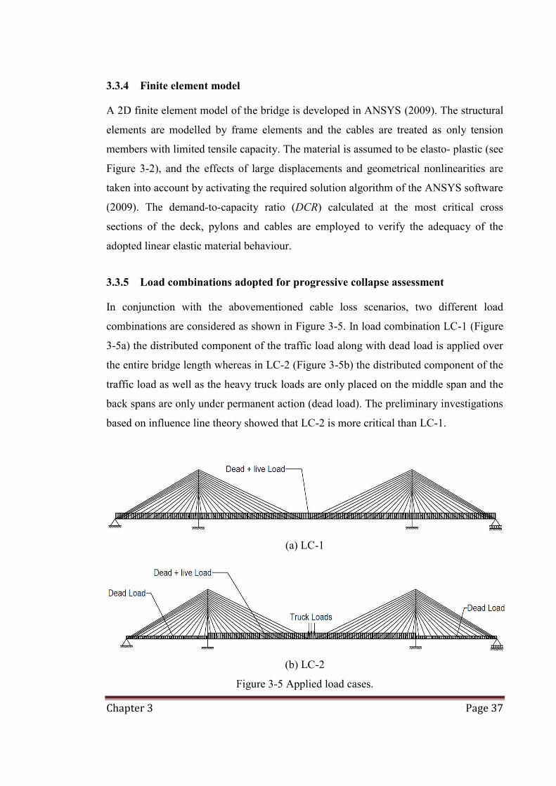
Chapter 3 Page 37

3.3.4 Finite element model

A 2D finite element model of the bridge is developed in ANSYS (2009). The structural

elements are modelled by frame elements and the cables are treated as only tension

members with limited tensile capacity. The material is assumed to be elasto- plastic (see

Figure 3-2), and the effects of large displacements and geometrical nonlinearities are

taken into account by activating the required solution algorithm of the ANSYS software

(2009). The demand-to-capacity ratio (DCR) calculated at the most critical cross

sections of the deck, pylons and cables are employed to verify the adequacy of the

adopted linear elastic material behaviour.

3.3.5 Load combinations adopted for progressive collapse assessment

In conjunction with the abovementioned cable loss scenarios, two different load

combinations are considered as shown in Figure 3-5. In load combination LC-1 (Figure

3-5a) the distributed component of the traffic load along with dead load is applied over

the entire bridge length whereas in LC-2 (Figure 3-5b) the distributed component of the

traffic load as well as the heavy truck loads are only placed on the middle span and the

back spans are only under permanent action (dead load). The preliminary investigations

based on influence line theory showed that LC-2 is more critical than LC-1.

(a) LC-1

(b) LC-2

Figure 3-5 Applied load cases.

Chapter 3 Page 38

For the cable loss scenarios, adopted load factors are as recommended by PTI (2007),

1.1DC + 1.35DW + 0.75 (LL+IM) +1.1CLDF (3-5)

where, DC= dead load of structural components and non-structural attachments, DW=

dead load of wearing surfaces and utilities, LL= full vehicular live load placed in actual

stripped lanes, IM= vehicular dynamic load allowance taken equal to zero in this study

and CLDF= cable loss dynamic forces.

In the example considered in this chapter, the exact value of cable internal forces are

available, and accordingly the load factor of 1.1 on the cable loss dynamic forces that

accounts for a variation of final cable force in construction has been ignored.

3.3.6 Cable removal method and type of analysis

In progressive collapse assessment of structures/bridges based on alternate load path

(ALP), the time over which the critical members (i.e. columns or cables) are removed

can significantly affect the response of the structures. If the member is removed over a

longer period of time (typically longer than the first natural period of structure) a static

analysis is deemed adequate, however, removing the members (i.e. columns or cables)

over a shorter period of time warrants a dynamic analysis. For analysis of cable stayed

bridges against progressive collapse, the cables can be removed through a static or

dynamic procedure and the FE model should be analysed accordingly. In this chapter,

for dynamic analysis a consistent mass matrix with a proportional damping is adopted

(Bathe, 1996) and Newmark constant acceleration method, which is unconditionally

stable, is used for time integration.

3.3.7 Discussion on the adequacy of the proposed 2D model

Due to lack of experimental data, the proposed 2D models in this study cannot be

validated directly; however, the adequacy and accuracy of the proposed FE models and

adopted constitutive laws for steel can be verified against other softwares and more

complex 3D finite element (FE) models.

Chapter 3 Page 39

In the first step, a 2D FE model of the bridge was developed using Microstran Software

and the results obtained from this model for the healthy bridge under LC-1 were

compared with the results obtained from 2D FE model developed in ANSYS software

(see Figure 3-6).

(a)

(b)

Figure 3-6 Comparison of results obtained from 2D models developed in (a) ANSYS

and (b) MicroStran for the healthy bridge under LC-1.

From this comparison, it can be observed that the response (including internal force in

the cables and towers and the maximum deflection at the mid-span) obtained from

ANSYS model correlates very well with Microstran results. In addition, a 3D FE model

of the bridge was developed using shell elements in ANSYS. In the 3D model all

material and geometrical nonlinearities were considered and element sizes varied

between 0.3-1.0 m. Outline of the 3D FE mesh is shown in Figure 3-7a. Regarding

material nonlinearity, Von Mises yield criterion with perfect plastic behaviour (i.e. no

strain hardening) was adopted (see Chapter 4). Comparison between 3D and 2D model

predictions for the healthy bridge under LC-1 is shown in Figures 3-7b and c that show

a very good correlation. Furthermore, comparison of 2D and 3D FE model predictions

for the mid-span deflection time history due to loss of cable no. 1 (under LC-1 load

case) is shown in Figure 3-8, that clearly demonstrates the adequacy of the proposed 2D

model for predicting the global response of the cable-stayed bridges.

max= -0.75

Ncable1=22,666 (kN) Ncable30=18,938 (kN)

Ncable1=20,744 (kN)

Ncable30=17,872 (kN)

Mbottom=258 (MN.m) Mbottom=712 (MN.m)

Mbottom=212 (MN.m) Mbottom=671 (MN.m) max= -0.75

Chapter 3 Page 40

(a)

(b)

(c)

Figure 3-7 Outline of the (a) 3D FE model and internal force and deflections predicted

by a (b) 2D linear-elastic model (c) 3D model with material & geometrical nonlinearity.

Figure 3-8 Time history of mid-span deflection predicted by 2D and 3D FE models for

the bridge subjected to loss of cable no. 1 and LC-1.

-2

-1.6

-1.2

-0.8

-0.4

00 5 10 15 20

Def

lect

ion

(m)

Time (sec)

3D

2D

Ncable1=20,744 (kN) Ncable30=17,872 (kN)

Total Reaction =519 (MN)

Ncable1a&b=19,262 (kN) Ncable30a&b=16,697 (kN)

Total Reaction =519 (MN)

max= -0.75

max= -0.67 (m)

Chapter 3 Page 41

3.4 Parametric studies and discussion

A parametric study is undertaken and parameters influencing DAF and DCR such as the

time over which the cable is removed, damping ratio and geometrical nonlinearities

(large displacements) are studied. Moreover, different cable loss scenarios are examined

and the most critical ones which lead to the maximum DAF and DCR are identified. The

results are presented in Tables 3-3 to 3-5. In these tables, ‘Ekill’ represents the

instantaneous removal of the cables over a time step, i.e. within 0.01 seconds.

3.4.1 Time step over which the cable is removed (cable removal time step)

For dynamic simulation of a cable loss scenario, the bridge without the lost cable is

modelled first and the initial force in the lost cable, initF , is gradually applied on the

tower and deck (see Figure 3-9a), then the bridge is allowed to reach the equilibrium

state which is basically equivalent to the healthy bridge.

After the bridge reaches the equilibrium state, the cable loss scenario is simulated by

reducing the force, initF , down to zero over a time step of ft (see Figure 3-9b).

Alternatively, the cable loss scenario can be achieved by activating a special solution

procedure in ANSYS by applying the "EKILL" command. It is noteworthy that the

EKILL command deactivates the lost cable element over an integration time step ( t

0.01 sec) whereby the element contributes a near-zero stiffness value to the overall

stiffness and mass matrix.

Since the time step over which the cable is removed, ft , can affect the dynamic

response of the bridge, in this part of the parametric study, sensitivity of the dynamic

response in relation to ft is examined. Four different cases corresponding to removal

of cable no. 30 (see Figure 3-9a) ft 8 sec, 1 sec, 0.1 sec and application of EKILL

command are considered (Figure 3-9b). The time history of bending moment in

scenario-1, case-3 at section C-C (Figure 3-3a) for four different cases (i.e. ft 8 sec,

1 sec, 0.1 sec and EKILL) are shown in Figure 3-10 and it is observed that dynamic

responses (particularly the maximum and minimum values) provided by different ft ,

Chapter 3 Page 42

more or less have the same magnitude except for the case in which the cable is removed

over 8 sec. The maximum DCR and corresponding DAF values calculated for one, two

and three cable loss scenarios are given in Tables 3-3 to 3-5, respectively.

Table 3-3 Maximum DCR and corresponding DAF values for scenario-1/LC-1 in which

one cable is lost (Gravity load case 1- critical damping ratio is taken as 0.5%).

Lost Cables No. Duration

ft(Sec)

Geometrical nonlinearity

DAF** (equivalent DAF) DCR*

1 (scenario-1/LC-1,

case-1, Section A-A)

8 on 1.1 (0.5) 40% off 1.1 (0.5) 40%

1 on 1.7 (0.8) 46% off 3.8 (1.8) 46%

0.1 on 1.8 (0.8) 48% off 7.9 (3.8) 48%

Ekill on 1.8 (0.8) 48%

15 (scenario-1/LC-1,

case-2, Section B-B)

8 on 1.7 (0.8) 28% off 2.4 (1.0) 28%

1 on 9.4 (4.1) 28% off 9.7 (4.3) 28%

0.1 on 60 (26)# 29% off 78 (35) # 29%

Ekill on 83 (36) # 30%

30 (scenario-1/LC-1,

case-3, Section C-C )

8 on 1.1 (0.6) 27% off 1.0 (0.5) 26%

1 on 2.4 (1.2) 30% off 2.0 (1.1) 29%

0.1 on 2.7 (1.3) 31% off 2.3 (1.4) 31%

Ekill on 2.6 (1.3) 31%

60 (scenario-1/LC-1,

case-4, Section D-D )

8 on 1.1 (0.6) 34% off 1.1 (0.5) 33%

1 on 1.6 (0.8) 39% off 1.6 (0.7) 37%

0.1 on 1.6 (0.9) 40% off 1.6 (0.7) 37%

Ekill on 1.7 (0.9) 40%

Chapter 3 Page 43

Table 3-4 Maximum DCR and corresponding DAF values for scenario-2/LC-2 in which

two cables are lost (Gravity load case 2- critical damping ratio is taken as 0.5%).

Lost Cables No. Duration tf (sec)

Geometrical nonlinearity

DAF** (equivalent DAF) DCR*

1&2 (scenario-2/LC-2,

case-1, Section A-A)

8 on 1.2 (0.6) 69% off 1.1 (0.5) 64%

1 on 2.7 (1.3) 84% off 14 (7.1) 74%

0.1 on 5.1 (2.4) 90% off 4.0 (2.0) 83%

Ekill on 5.7 (2.7) 91%

30&31 (scenario-2/LC-2,

case-2, Section C-C)

8 on 1.9 (0.7) 45% off 1.0 (1.0) 44%

1 on 20# (7.5) 60% off 1.1 (1.1) 59%

0.1 on 35# (13) 64% off 1.3 (1.3) 64%

Ekill on 36# (14) 63%

* DCR values are calculated based on combination of axial force and bending moment at different critical sections (with maximum bending moment) along the deck (see Figure 3-3a for location of critical sections).

** DAF values were calculated based on maximum bending moment except the ones with # superscript.

# DAF value was calculated based on maximum axial force and is a large value due to small static response.

Chapter 3 Page 44

Table 3-5 Maximum DCR and corresponding DAF values for scenario-3/LC-2 in which

three cables are lost (Gravity load case 2).

Lost Cables No. Duration tf (sec)

Geometrical nonlinearity Damping DAF**

(equivalent DAF) DCR*

1 & 2 & 3 (scenario-3/LC-

2, case-1, Section A-A)

8 on

0.5%

1.2 (0.7) 81% off 1.1 (0.6) 78%

1 on 1.9 (1.1) 108% off 1.8 (0.9) 104%

0.1 on 3.1 (1.4) 117% off 2.4 (1.2) 111%

Ekill on 3.2 (1.5) 120%

8 on

1.0%

1.2 (0.7) 81% off 1.1 (0.6) 78%

1 on 1.9 (1.1) 107% off 1.8 (0.9) 104%

0.1 on 2.5 (1.2) 114% off 1.9 (1.0) 109%

Ekill on 2.7 (1.2) 116%

8 on

2.0%

1.2 (0.7) 80% off 1.1 (0.6) 78%

1 on 1.9 (1.1) 106% off 1.8 (0.9) 102%

0.1 on 2.0 (1.2) 110% off 1.9 (1.0) 106%

Ekill on 2.0 (1.2) 112%

With regard to Tables 3-3 to 3-5, it is observed that DAF and DCR values are quite

sensitive to ft (particularly when two cables are lost) and for accurate estimation of

DAF and DCR a fairly small ft ( about 0.001-0.1 sec) is required, which is consistent

with the recommendations of some guidelines for progressive collapse analysis of

framed structures (DoD, 2005, GSA, 2003). It should be noted that removing the cable

over 8 sec or 1 sec in this example cannot adequately simulate the sudden loss of cable

and produces a quasi-static scenario rather than a dynamic one.

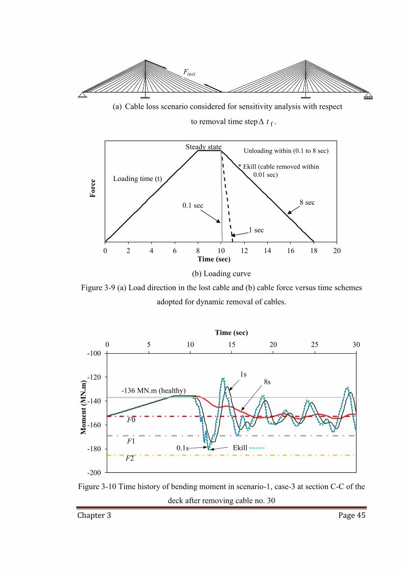
Chapter 3 Page 45

(a) Cable loss scenario considered for sensitivity analysis with respect

to removal time step ft .

(b) Loading curve

Figure 3-9 (a) Load direction in the lost cable and (b) cable force versus time schemes

adopted for dynamic removal of cables.

Figure 3-10 Time history of bending moment in scenario-1, case-3 at section C-C of the

deck after removing cable no. 30

0 2 4 6 8 10 12 14 16 18 20

Forc

e

Time (sec)

-200

-180

-160

-140

-120

-1000 5 10 15 20 25 30

Mom

ent (

MN

.m)

Time (sec)

-136 MN.m (healthy)

F0

8s

Ekill

1s

0.1s F1

F2

8 sec

1 sec

0.1 sec

* Ekill (cable removed within 0.01 sec) Loading time (t)

Steady state Unloading within (0.1 to 8 sec)

initF

Chapter 3 Page 46

3.4.2 Structural damping

Mozos and Aparisio (2010b) identified the structural damping ratio as one of the factors

that can significantly influence the progressive collapse response of the bridge and DAF

values, however, they do not provide any details in this regard. Accordingly, the

importance of damping ratio and its impact on DAF and DCR values are investigated in

this section. For parametric study, three different levels of damping, i.e. 0.5%, 1% and

2% of critical damping within the acceptable range for steel structures are adopted

(Clough and Penzien, 1993). For the triple cable loss scenario, i.e. scenario-3, the time

history of bending moment at Section A-A (refer to Figure 3-3a) for three different

levels of damping (i.e. 0.5%, 1% and 2% of critical damping) are shown in Figure 3-11

and it is observed that the time history and the maximum/minimum values are very

similar for all adopted damping ratios.

The maximum DCR and corresponding DAF values calculated for the scenarios with

three cable losses are given in Table 3-5. The results provided in Table 3-5 clearly show

that DAF and DCR values are not sensitive to the level of damping ratio adopted for

dynamic analysis. Furthermore, it can be concluded that the damping ratio within the

range considered (i.e. 0-2% of critical damping), has a minor impact on the potential

progressive collapse response of the cable stayed bridges.

Figure 3-11 Time history of bending moment in scenario-3 at section A-A of the deck

obtained from dynamic analysis with different damping ratios.

-600

-500

-400

-300

-200

-100

00 5 10 15 20 25 30

Mom

ent (

MN

.m)

Time (sec)

2% (-473 MN.m)

1% (-487 MN.m)

0.5% (-499 MN.m)

-150 MN.m (healthy)

Chapter 3 Page 47

3.4.3 Geometrical nonlinearities

Effect of geometrical nonlinearity should be taken into account when the deflections of

the structure are large enough compared with the size of structural members.

Furthermore, for compressive structural members such as columns or pylons the second

order P effects can reduce the stiffness and loading capacity of the members,

particularly in cable stayed bridges, the P effects can be quite significant for

pylons/towers subjected to lateral air blast pressure (Son and Lee, 2011). The general

understanding is that during cable loss scenarios, geometrical nonlinearities can affect

the response of the cable stayed bridges and therefore they should be taken into account

(Mozos and Aparicio, 2010a, Wolff and Starossek, 2010), however, there is no

comprehensive study to clearly demonstrate the contribution of the geometrical

nonlinearities to DAF values and the progressive collapse response of the cable stayed

bridges. The maximum DAF and DCR values calculated for different cable loss

scenarios with and without geometrical nonlinearities included are summarised in

Tables 3-3 to 3-5. It is observed that for the bridge under consideration, the effect of

geometrical nonlinearities on DAF is considerable and the major contribution of

geometrical nonlinearity to DAF comes from the dynamic analysis )(tdynS ; in particular,

inclusion of geometrical nonlinearities for scenario-1, case-1 in which cable No. 1 is

lost has led to a 200% to 400% increase in DAF. Among investigated cable loss

scenarios, the scenarios involving loss of cable No. 1 (back stay connected to the hinge

support) are the most critical ones in terms of significance of geometrical nonlinearity.

With regard to Tables 3-3 to 3-5 it is concluded that the maximum and minimum DCR

values for towers, deck and cables are not really sensitive to geometrical nonlinearity

and geometrical nonlinearities have a minor role (for this example less than 7%) in

driving the structural members towards their ultimate state during cable loss scenarios.

3.4.4 Cable removal scenarios

In this part, dynamic progressive collapse response of the bridge due to different cable

loss scenarios is investigated. The configuration of gravity load cases applied on the

deck is shown in Figure 3-5 and a constant damping of 0.5% of critical damping is

adopted for dynamic analyses.

Chapter 3 Page 48

Single cable loss

For the sake of comparison, in the single cable loss scenarios two different gravity load

cases (i.e. LC-1 and LC-2) are considered (Figure 3-5).

LC-1

Figure 3-12 shows the time history of the bending moment at section E-E, which is the

bottom of left tower (see Figure 3-3a), for different cases within scenario-1/LC-1, in

which cables no.1, 15, 30 and 60 are removed. It is observed that loss of cables 1, 30

and 60 can significantly affect the magnitude of bending moment at the bottom of left

tower, whereas loss of cable no.15 has a minor effect. Among four different cases

considered under scenario-1/LC-1, loss of cable no.1 (the longest back stay) is the most

critical in terms of maximum bending moment induced in the bottom of the tower.

For scenario-1/LC-1, the value of DAF and DCR, calculated based on maximum

bending moment at the most critical sections along the deck (see Figure 3-3a) are given

in Table 3-3. Furthermore, the maximum DCR values and corresponding DAF observed

in the deck, towers and cables for scenario-1/LC-1 are given in Table 3-6. With regards

to Table 3-6, it can be concluded that DAF can take values higher than 2.0, however the

DCR values are still well below 100% (no yielding has occurred).

Figure 3-12 Time history of bending moment at the bottom of the left tower for

different cable loss cases under scenario-1/LC-1 (only one cable is lost).

-800

-600

-400

-200

0

200

4000 5 10 15 20 25 30

Mom

ent (

MN

.m)

Time (sec)

case-1 (no.1)

-56 MN.m (healthy)

case-3 (no.30) case-4 (no.60)

case-2 (no.15)

Chapter 3 Page 49

In addition, for all structural components, it is concluded that loss of cables no. 1 and 30

are more critical than the other cases under scenario-1/LC-1 and accordingly for

scenario-1/LC-2 only loss of these cables will be considered.

Table 3-6 Maximum DCR and corresponding DAF values in towers, deck and cables

under scenario-1/LC-1 (Gravity load case 1 – critical damping ratio is taken as 0.5%).

Lost Cables No. Component DAF (equivalent DAF) DCR

1 (scenario-1/LC-1,

case-1)

Left tower (bottom) 2.3 (1.1) 25%

Right tower (bottom) 6.8 (3.0) 25%

Deck (section A-A) 1.8 (0.8) 48%

Cable (Cable no. 2) 1.7 (0.8) 36%

15 (scenario-1/LC-1,

case-2)

Left tower (bottom) 8.2 (4.7) 14%

Right tower (bottom) 122# (30#) 14%

Deck (section B-B) 83# (36#) 30%

Cable (cable no. 14) 1.9 (1.0) 40%

30 (scenario-1/LC-1,

case-3)

Left tower (bottom) 2.6 (1.4) 18%

Right tower (bottom) 2.7 (1.3) 18%

Deck (section C-C) 2.7 (1.3) 31%

Cable (cable no. 31) 1.5 (0.7) 33%

60 (scenario-1/LC-1,

case-4)

Left tower (bottom) 7.8 (4.1) 18%

Right tower (bottom) 1.2 (0.6) 17%

Deck (section D-D) 1.7 (0.9) 40%

Cable (cable no. 59) 1.6 (0.8) 35%

# DAF value was calculated based on maximum axial force and is a large value due to small static response.

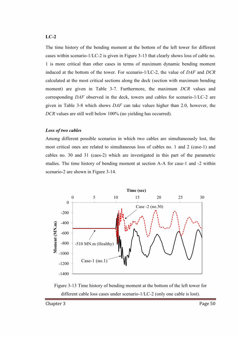
Chapter 3 Page 50

LC-2

The time history of the bending moment at the bottom of the left tower for different

cases within scenario-1/LC-2 is given in Figure 3-13 that clearly shows loss of cable no.

1 is more critical than other cases in terms of maximum dynamic bending moment

induced at the bottom of the tower. For scenario-1/LC-2, the value of DAF and DCR

calculated at the most critical sections along the deck (section with maximum bending

moment) are given in Table 3-7. Furthermore, the maximum DCR values and

corresponding DAF observed in the deck, towers and cables for scenario-1/LC-2 are

given in Table 3-8 which shows DAF can take values higher than 2.0, however, the

DCR values are still well below 100% (no yielding has occurred).

Loss of two cables

Among different possible scenarios in which two cables are simultaneously lost, the

most critical ones are related to simultaneous loss of cables no. 1 and 2 (case-1) and

cables no. 30 and 31 (caes-2) which are investigated in this part of the parametric

studies. The time history of bending moment at section A-A for case-1 and -2 within

scenario-2 are shown in Figure 3-14.

Figure 3-13 Time history of bending moment at the bottom of the left tower for

different cable loss cases under scenario-1/LC-2 (only one cable is lost).

-1400

-1200

-1000

-800

-600

-400

-200

00 5 10 15 20 25 30

Mom

ent (

MN

.m)

Time (sec)

Case -2 (no.30)

Case-1 (no.1)

-510 MN.m (Healthy)

Chapter 3 Page 51

Table 3-7 Maximum DCR and corresponding DAF values for scenario-1/LC-2 in which

one cable is lost (Gravity load case 2 - critical damping ratio is taken as 0.5%).

Lost Cables No. Duration tf (sec)

Geometrical nonlinearity

DAF (equivalent DAF) DCR

1 (scenario-1/LC-2,

case-1, Section A-A)

8 on 1.1 (0.6) 55% off 1.0 (0.5) 52%

1 on 4.0 (2.0) 62% off 3.0 (1.6) 57%

0.1 on 7.1 (3.7) 63% off 6.1 (3.2) 60%

Ekill on 8.2 (4.2) 64%

30 (scenario-1/LC-2,

case-2, Section C-C)

8 on 1.1 (0.6) 43% off 1.1 (0.5) 40%

1 on 2.4 (1.2) 47% off 2.3 (1.0) 44%

0.1 on 2.8 (1.3) 49% off 3.0 (1.3) 46%

Ekill on 2.7 (1.3) 49%

Table 3-8 Maximum DCR and corresponding DAF values in towers, deck and cables

under scenario-1/LC-2 (Gravity load case 2 - critical damping ratio is taken as 0.5%).

Lost Cables No. Component DAF (equivalent DAF) DCR

1 (scenario-1/LC-2,

case-1)

Left tower (bottom) 2.4 (0.8) 36%

Right tower (bottom) 0.6 (0.3) 37%

Deck (section A-A) 8.2 (4.2) 64%

Cable (cable no.2) 1.1 (0.6) 38%

30 (scenario-1/LC-2,

case-2)

Left tower (bottom) 8.2 (0.9) 27%

Right tower (bottom) 0.6 (1.2) 17%

Deck (section C-C) 2.8 (1.3) 49%

Cable (cable no.31) 2.3 (1.1) 36%

Chapter 3 Page 52

Figure 3-14 Time history of the bending moment at section A-A of the deck under

scenario-2/LC-2 (two cables are lost).

It is observed that scenario-2/case-1 corresponding to loss of two back stays (cables no.

1 and 2) is the most critical one in terms of maximum dynamic bending moment

induced in the deck. Accordingly, the maximum DCR values and corresponding DAF

observed at different locations in the deck, towers and cables for scenario-2/case-1 are

given in Figure 3-15.

Moreover, for scenario-2/LC-2, DAF and DCR values determined at the most critical

sections (based on maximum bending moment) along the deck are given in Table 3-4.

With regard to the results obtained for scenario-2, it is concluded that similar to

scenario-1, DAF can take values higher than 2.0, however the DCR values are still

below 100% (no yielding has occurred) and accordingly no potential progressive

collapse due to material nonlinearity is expected.

-400

-350

-300

-250

-200

-150

-100

-50

00 5 10 15 20 25 30

Mom

ent (

MN

.m)

Time (sec)

Case-2 (no.30 & 31 are lost)

Case-1 (no.1 & 2 are lost)

-150 MN.m (healthy)

Chapter 3 Page 53

Figure 3-15 DAF versus DCR values for scneaio-2 (LC-2, loss of cables no. 1 and 2).

Figure 3-16 DAF versus DCR values for scneaio-3 (LC-2, loss of cables no. 1, 2 & 3).

0%

50%

100%

0 1 2 3 4 5

DC

R

DAF

Left tower max momentmin momentmax axial forcemini axial force

0%

50%

100%

0 1 2 3 4 5

DC

R

DAF

Deck max momentmin momentmax axial forcemini axial force

0%

50%

100%

0 1 2 3 4 5

DC

R

DAF

Left tower max momentmini momentmax axial forcemini axial force

0%

50%

100%

0 1 2 3 4 5

DC

R

DAF

Deck max momentmini momentmax axial forcemini axial force

0%

50%

100%

0 1 2 3 4 5

DC

R

DAF

Right tower max momentmin momentmax axial forcemini axial force

0%

50%

100%

0 1 2 3 4 5D

CR

DAF

Cables max axial forcemini axial force

0%

50%

100%

0 1 2 3 4 5

DC

R

DAF

Right tower max momentmini momentmax axial forcemini axial force

0%

50%

100%

0 1 2 3 4 5

DC

R

DAF

Cables max axial forcemini axial force

Chapter 3 Page 54

Loss of three cables

With regard to the results obtained from the previous scenarios, it can be concluded that

scenarios associated with loss of back stays connected to the pin support are the most

critical ones. Accordingly, simultaneous loss of cables no. 1, 2 and 3 is only considered

in this part. For scenario-3/LC-2, DAF and DCR values determined based on maximum

bending moment at the most critical sections along the deck are given in Table 3-5. In

addition, the maximum DCR and corresponding DAF values observed in the deck,

towers and cables for scenario-3/LC-2 are given in Figure 3-16. The maximum DAF

calculated within this scenario is about 4.5 and related to the maximum moment in the

right tower. In scenario-3, DCR takes values greater than 100% (yielding may occur due

to combination of bending moment and axial load in the deck, see Table 3-5). However,

even in the event of formation of a plastic hinge at one location of the deck, the

redundancy provided by the supports through the remainder of the cables will prevent

the progressive collapse of the bridge.

3.5 Concluding remarks

A numerical study on the potential progressive collapse of cable stayed bridges due to

different cable loss scenarios was carried out in this chapter. A comprehensive

parametric study was undertaken and effect of location, duration and number of lost

cables, as well as applied load case and the structural damping ratio on the dynamic

amplification factor (DAF) and demand-to-capacity ratio (DCR) in different structural

members (towers, deck and cables) are investigated. With regard to the parametric

studies undertaken in this chapter, the following conclusions are drawn;

- Among different cable loss scenarios considered for potential progressive collapse

of the cable stayed bridge, the ones associated with loss of the longest back stays are

the most critical ones (the highest DCR values were observed for all structural

components).

- The DAF for the bending moment and axial force at different sections along the

Chapter 3 Page 55

deck, towers and cables can take values much higher than 2 (typically adopted by

different guidelines as the maximum value), however, the corresponding DCR

values were usually less than 100%. In other words, material nonlinearity has minor

effect on the global progressive collapse response of the bridge due to cable loss,

and it is not un-conservative to allow a DAF of greater than 2 as long as DCR

remains below 1.

- The DAF values alone, do not provide any information about the progressive

collapse response of the cable stayed bridge under investigation, whereas DCR

values at different locations of the structure can be used as an indicator of material

nonlinearity and formation of plastic hinges.

- Damping ratio has a minor impact on the dynamic progressive collapse response of

the cable stayed bridges as long as the adopted value of the damping ratio is within

the acceptable range (less than 2% of critical damping for the steel bridge

considered in this study).

- The developed FE model for the bridge was analysed with and without geometrical

nonlinearities included to demonstrate the effect of geometrical nonlinearities on the

global progressive collapse response of the bridge. It was shown that for the cases

studied in this paper, the effect of geometrical nonlinearities on the progressive

collapse response (due to cable loss), for a properly designed bridge is limited (less

than 7% for the cases considered in this study).

- The value of DAF is highly sensitive to the time step over which the cables are

removed.

- The value of DAF for bending moment and axial force in the towers and deck is

larger than the DAF that should be applied for axial force in the cables.

- For all cases and scenarios studied in this chapter, values of DAF for axial force in

the cables are generally less than 2.

Chapter 4 Page 56

Chapter 4 : Model verification - A Comparative

Study of 2D and 3D FE Models of a Cable-Stayed

Bridge Subjected to Sudden Loss of Cables Summary of chapter

In the previous chapter, DAFs and DCRs were determined by using 2D linear elastic models,

mainly because the sudden loss of cables is typically analysed by 2D linear-elastic models in

design of cable-stayed bridges. However, cable loss scenarios are associated with material as well

as geometrical nonlinearities which may trigger progressive collapse of the entire bridge.

Accordingly, a non-linear 3D bridge model is required to adequately investigate the cable loss

scenarios. The non-linear 3D model to be developed in this chapter can be used to analysis the

unsymmetrical cable loss scenarios as well as loss of cables subject to blast loading. However, this

chapter only focus on the correlation between results of nonlinear 3D and 2D linear-elastic finite

element (FE) models. The results of this comparative study are employed to determine the

adequacy of linear elastic models for potential progressive collapse assessment of cable stayed

bridges. In this chapter, 2D and 3D finite element models of a cable-stayed bridge with and

without considering material and geometrical nonlinearities are developed and analysed. The

progressive collapse response of the bridge subjected to two different cable loss scenarios at

global and local levels are investigated. For the cases studied in this chapter, it is shown that the

linear elastic 2D FE models can adequately predict the dynamic response (i.e. deflections and

main stresses within the deck, tower and cables) of the bridge subjected to cable loss. Material

nonlinearities occurred at different locations are found to be localized and unlikely to trigger the

progressive collapse of the entire bridge.

4.1 Introduction

The finite element models employed for progressive collapse analysis of structures can

be classified to 2D or 3D models. The 2D models have been successfully used for

capturing the global response of the cable-stayed bridges as well as identifying the most

Chapter 4 Page 57

critical structural components. For example, using a 2D finite element (FE) model, the

back stays connected around the pin-support and also the stays connected to the mid-

span have been identified as the most critical cables as presented in the previous chapter

as well as previous studies (Aoki et al., 2012a, Aoki et al., 2012b, Kao and Kou, 2010).

The 2D models, however, cannot capture the effects of out-of-plane unsymmetric cable

loss scenarios that may have a significant influence on the response (particularly the

torsional response) of the bridges.

The cable-stayed bridge adopted in this study has a steel box deck designed according

to Australian Standards AS5100 (2004) requirements. The 2D and 3D FE models of the

bridge were developed and analysed under gravity loads and subjected to different cable

loss scenarios using SAP2000 (2004) and ANSYS software (2009), respectively. The

nonlinear 3D FE models are developed to provide the benchmark data required for

assessing the accuracy of 2D FE models commonly developed assuming a linear elastic

material behaviour. The developed 3D FE models can take account of material non-

linearity as well as geometrical non-linearity. Using the 2D and 3D FE models, the

effect of location of lost cables on the potential collapse response of the bridge is

studied and also the significance of material nonlinearities on the potential collapse

response of the considered cable stayed bridge is investigated.

4.2 Principal Assumptions

4.2.1 Geometry and material properties

The dimensions of the bridge and the configuration of cables for the bridge considered

in this chapter are the same as the bridge used in Chapter 3 as shown in Figure 4-1a.

The cross sectional area of deck and towers has been re-designed in order to prevent

premature local buckling of plates before yielding of steel. The slenderness of

unsupported length of plates, 250/)/( ytb , was limited to the yield limit slenderness

ratio ey (45 for plates supported on one edge and 32 for plates supported on both edges

of deck) according to AS 5100.6 (2004) requirements. The geometry of the deck, towers

and configuration of cables are shown in Figure 4-1b and 4-1c, respectively.

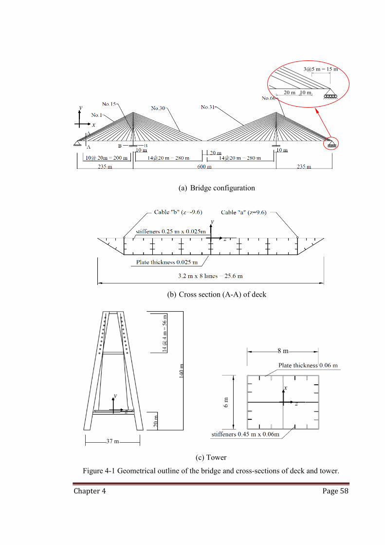
Chapter 4 Page 58

(a) Bridge configuration

(b) Cross section (A-A) of deck

(c) Tower

Figure 4-1 Geometrical outline of the bridge and cross-sections of deck and tower.

z

y

x

y

3@5 m = 15 m

10 m20 m

11.5 m

z

y

8 m

z

x

37 m

Chapter 4 Page 59

The adopted material properties (i.e. uyE ,, and shE ), initial post-tensioning strain in

cables PTi , and the geometrical properties of members (i.e. cables, deck and tower)

including second moment of area, I , and cross sectional area, A adopted in 2D FE

models are given in Table 4-1. The material is assumed to be linear elastic in 2D

models, whereas in 3D models a linear elasto-plastic hardening stress-strain relationship

with Von Mises yield surface is adopted for deck and tower (Figure 4-2a). The cables

are assumed to be linear elastic-brittle in 2D and 3D FE models (Figure 4-2b).

(a) (b)

Figure 4-2 Adopted stress-strain model for steel in the (a) tower and deck and

(b) cables.

Table 4-1 Material and geometrical properties of the deck, towers and cables.

Structural component (MPa)

E (MPa)

y (MPa)

u (MPa)

shE )(m 2

A

)(m 4

I PTi

Box Girder 200 350 420 500 1.91 1.36 -

Tower 200 350 420 500 6.09 47.41 -

Cable No.

1-5, 26-35, 56-60 200 1860 1860 - 0.0327 - 0.0033 6-10,21-25,36-40,

51-55 200 1860 1860 - 0.0219 - 0.0033

11-20, 41-50 200 1860 1860 - 0.0165 - 0.0037

# E is the modulus of elasticity, y and u denote the yield and ultimate strength and Esh is the hardening

modulus of steel.

0

100

200

300

400

500

600

0 30 60 90 120 150

Stre

ss (M

Pa)

Strain x 10-3 (mm/mm)

0

500

1000

1500

2000

0 2 4 6 8 10

Stre

ss (M

Pa)

Strain x 10-3 (mm/mm)

Linear elasto-plastic hardening

Linear elastic-brittle

Chapter 4 Page 60

4.2.2 Modelling and analysis

For both static and dynamic analyses of the cable stayed bridge under investigation, the

effects of large displacements and geometrical nonlinearities are taken into account in

both 2D and 3D FE models. Furthermore, in the dynamic analysis, a proportional

damping with stiffness and mass multipliers of %5.0 is adopted (Clough and

Penzien, 1993).

In the 3D FE model, the deck and towers are modelled by shell elements, whereas 2D

FE models take advantage of beam elements. The cables are modelled by link-elements

which are treated as tension-only members with limited tensile capacity. The outline of

the 2D and 3D FE models are shown in Figure 4-3. In the 2D models, the eccentricity of

cables with respect to the centroidal axis of the deck and pylons was modelled by rigid

constraints (see Figure 4-3a).

(a) 2D model

(b) 3D model

Figure 4-3 Outline of the (a) 2D and (b) 3D finite element model.

Pylon

Deck Cable

Chapter 4 Page 61

In this research project, shell element SHELL181, which is suitable for analysing thin to

moderately-thick shell structures is used for modelling steel plates. SHELL181 is a

four-node element with six degrees of freedom at each node. Also, SHELL181 is well-

suited for linear, large rotation, and/or large strain nonlinear applications. This element

supports uniform reduced integration, full integration, and full integration with

incompatible modes. In this research, full integration (five points of integration through

the thickness of the shell) is used.

In addition, for SHELL181 element, the default orientation has shell surface coordinate

(called as S1) axis aligned with the first parametric direction of the element at the centre

of the element. In the most general case, the S1 axis can be defined as follows

sxsx

S1 (4-1)

where

LKJI xxxxsx

41 (4-2)

and LKJI xxxx and,, are global coordinates of the nodal points.

In the 3D continuum-based FE models, LINK10 is used for modelling cables. It is a 3D

spar element having the unique feature of a bilinear stiffness matrix resulting in a

uniaxial tension-only element. With this option, the stiffness is removed if the element

goes into compression (simulating a slack cable or slack chain condition. LINK10

element has three degrees of freedom at each nodal point. No bending stiffness is

included in the LINK10 element that is consistent with the real behaviour of cables.

Chapter 4 Page 62

4.2.3 Design Loads

The loads considered for collapse assessment of this bridge are gravity loads including

the self-weight of the structure (Dead) plus the surfacing asphalt (Superimposed Dead)

and the traffic load (S1600 as shown in Figure 4-4) according to AS5100.2 (2004).

Figure 4-4 S1600 stationary traffic load according to AS5100 (2004).

Applied post-tensioning forces in the cables were calculated according to AS5100.2

(2004) provisions for ultimate and serviceability design requirements as well as

allowable mid-span deflection due to traffic loads. Further, the maximum stress induced

in the deck and towers due to service load (i.e. Permanent + Traffic + Post-tensioning

forces) was kept below y5.0 and the maximum stress in the cables is limited to that

considered consistent with JSCE (2010) design provisions.

4.2.4 Calibration of 2D and 3D FE models

The correlation between the 2D and 3D FE models developed in this study was verified

by comparing the total self-weight, cable initial forces and global deflection of the deck

obtained from the FE models. The total weight of the bridge obtained from 2D and 3D

FE models under progressive collapse load combination of (1.1xDead +

1.35xSuperimposed Dead + 0.75xTraffic) are 647 MN and 656 MN, respectively.

Furthermore, the vertical deflection, the stress in the cables and xx stress on top

surface of the bridge deck obtained from 2D and 3D FE models are compared in Figure

4-5 that demonstrates a good correlation between 2D and 3D FE results. The xx stress

Chapter 4 Page 63

at each section in 2D FE models were calculated from IMyANxx // ; where N and

M are the axial force and bending moment, respectively, y is the distance from the

neutral axis and A denotes the cross-sectional area and I denotes the moment of inertia

of the section (see Table 4-1).

(a) Vertical displacements along the deck

(b) Ratio of the axial force (stress) over breakage load (stress) for stays (under

service load).

(c) xx Stress component on top surface of the deck.

Figure 4-5 Comparison between results of 2D and 3D finite element models.

-1.0

-0.5

0.0

0.5

0 100 200 300 400 500 600 700 800 900 1000

Ver

tical

def

lect

ion

(m)

2D Model3D Model

0%

10%

20%

30%

40%

50%

0 10 20 30 40 50 60

Stre

ss r

atio

Cable no.

2D Model3D Model

-120

-80

-40

0

40

80

0 100 200 300 400 500 600 700 800 900 1000

xx t

op o

f dec

k (M

Pa) 2D Model

3D Model

Chapter 4 Page 64

In addition, the periods of the first five in-plane natural vibration modes obtained from

Eigen value analyses of the 2D and 3D FE models are given in Table 4-2 and a

maximum of 13% difference between the 2D and 3D FE predictions is observed. For

all modes of vibrations, the periods associated with the 3D model are smaller than those

for the 2D model.

During the process of modelling and calibration of 2D versus 3D models, the

eccentricity of cables with respect to the centroidal axis of the deck and towers was

found to be important and accordingly should be considered for proper calibration of

the 2D FE models (see Figure 4-3a).

Table 4-2 The periods of the first five in-plane global natural modes of vibration.

Mode no. 2D Model (sec) 3D Model (sec) 1st 5.68 5.15 2nd 4.59 4.22 3rd 2.95 2.64 4th 2.63 2.36 5th 2.51 2.22

4.3 Cable Loss Scenarios

4.3.1 Cable removal method

For dynamic analysis, the unconditionally stable Newmark constant acceleration

method is used for time integration (Paz, 2004). The cables are removed over an

integration time step, t , which is short enough compared with the 1st natural period of

the bridge to warrant the adequacy of dynamic analysis for alternate load path (ALP)

method (Ellingwood et al. 2007).

4.3.2 Load combinations adopted for progressive collapse assessment

For collapse assessment, the distributed component of the traffic load, as well as the

dead load, is applied along the entire bridge deck (Figure 4-6a). The adopted load

factors are as recommended by PTI (2007),

CLDFIMLLDWDC 1.1)(75.035.11.1 (4-3)

Chapter 4 Page 65

(a) UDL along the deck

(b) Symmetric loading pattern

Figure 4-6 Pattern of (a) gravity loads along the bridge deck (Dead + traffic)

(b) traffic loads across the deck including accompanying lane factors for

progressive collapse assessment

In Equation (4-3), DC is the dead load of the structural components and non-structural

attachments, DW is the dead load of the wearing surfaces and utilities, LL is the full

vehicular live load placed in the actual stripped lanes, IM denotes the vehicular dynamic

load allowance taken equal to zero in this study and CLDF is the cable loss dynamic

forces. In this study, the wearing surface is a 200 mm thick layer of asphalt concrete

(γ=24.5 kN/m3). According to AS5100.2 (2004), for scenarios in which more than one

lane is subjected to traffic loads, applied traffic loads should be multiplied by an

accompanying lane factor (1.0 for first lane, 0.8 for second lane and 0.4 for third and

subsequent lanes (see Figure 4-6b).

4.3.3 Cable loss scenarios

Based on PTI (2007) guidelines, for progressive collapse assessment of cable stayed

bridges, only the scenarios associated with loss of a single cable are adequate, however,

some researchers believe that scenarios in which more than one cable is lost should not

be ignored (Aoki et al., 2011, Wolff and Starossek, 2010). Two different scenarios (i.e.

S1 and S2) which are considered to be the most critical ones (see Chapter 3) are studied

here. In the 2D model, cable no.1 (connected to the pin support) and cable no.30 (the

Chapter 4 Page 66

longest cable connected to the mid-span) are subject to loss. These scenarios are

referred to as scenario-S1 (2D) and scenario-S2 (2D), respectively. The corresponding

symmetrical cable loss scenarios in 3D FE models are scenario-S1 (3D) and S2 (3D) in

which a pair of cables (1a and 1b) and (30a and 30b) are simultaneously removed (see

Figure 4-1a). The considered cable loss scenarios are listed in Table 4-3.

Table 4-3 Cable loss scenarios considered in this chapter.

Scenario name

Lost cable no.

Model type 2D/3D

Cable loss pattern

Traffic loading pattern

S1(2D)-SL 1 2D Symmetric

Symmetric

Symmetric (see Figure 4-6b)

S2(2D)-SL 30 S1(3D)-SL 1a & 1b

3D S2(3D)-SL 30a & 30b

4.3.4 Equivalent Modulus of Elasticity for Cables

The shape (geometry) of stays in cable-stayed bridges can change due to variation of

stress levels and a simple approach to account for this geometrical nonlinearity is to

adjust the modulus of elasticity (JSCE, 2010, Walther, 1999, Gimsing and Georgakis,

2011). The equivalent modulus of elasticity is determined by the following equation

which was established by H.J. Ernst (JSCE, 2010, Walther, 1999)

2

3112

EEl E

(4-4)

where, E is the equivalent modulus of elasticity, E is material modulus of elasticity,

is density of the cable, l is the horizontal span (x coordinate) and is the stress in the

cable. For the longest cable connected to the mid-span, GPa200eE , 3m/kN78 ,

m314l and MPa61333.0 u , the equivalent modulus of elasticity is

eEE 96.0 that would have small effect on the results and, hence, actual modulus value

(instead of the equivalent modulus) is used in subsequent analyses.

Chapter 4 Page 67

4.4 Results

Analysis results for symmetrical cable loss scenarios S1 and S2 obtained from 2D and

3D FE models are compared in this section.

4.4.1 Deck and Towers

Time-history of vertical deflection at the mid-span of deck (i.e. x=535 m) and xx

stress component on top and bottom of the deck (at the maximum stress instant) for

scenarios S1 and S2 are shown in Figures 4-7 and 4-8, respectively.

The magnitude and location of maximum vertical deflection within the deck as well as

the maximum xx longitudinal stress on top and bottom surface of the deck obtained

from 2D and 3D FE models are compared in Table 4-4. It is observed that the difference

between 2D and 3D FE models in terms of predicted xx stress is limited to 8% and for

predicted deflections the maximum difference between 2D and 3D model is around 6%.

Furthermore, it is seen that the major longitudinal flexural stresses along the deck (see

Table 4-4) are well below the yield strength of steel, i.e. MPay 350 and accordingly

neither cable loss scenario S1 nor S2 will lead to formation of plastic hinge along the

deck. The deflected configuration (elastic curve) of the deck at the maximum vertical

displacement instant for scenarios S1 and S2 is shown in Figure 4-9a and time history

and maximum lateral drift on top of left tower obtained from 2D and 3D models are

compared in Figure 4-9b and Table 4-4, respectively. It is observed that the calibrated

2D model can adequately capture the global response (i.e. deflection and major flexural

stresses in the deck and towers) of the bridge during cable loss scenarios.

Table 4-4 Material and geometrical properties of the deck, towers and cables.

Scenario (FE model)

Deflection in deck (m) Max. drift on top of the left

tower (m)

Max. xx stress in deck (MPa)

Mid span Max. @ x (m) Top of deck Bottom of deck

S1 (2D) 1.81 2.04 @ 485 0.69 137 233 S1 (3D) 1.88 2.17 @ 485 0.68 129 227 S2 (2D) 1.83 1.86 @ 530 0.16 55 185 S2 (3D) 1.86 1.81 @ 540 0.16 51 206

Chapter 4 Page 68

(a)

(b)

(c)

Figure 4-7 Time history of (a) vertical deflection at mid-span (x= 535 m) and xx stress

component on the (b) top and (c) bottom surface of the deck for scenario-S1.

-2

-1.6

-1.2

-0.8

-0.40 5 10 15 20 25 30

Ver

tical

def

lect

ion

(m)

Time (sec)

2D Model3D Model

-150

-100

-50

0

50

100

150

0 200 400 600 800 1000

xx t

op o

f dec

k (M

Pa) 2D Model

3D Model

-300

-200

-100

0

100

200

0 100 200 300 400 500 600 700 800 900 1000

xx b

otto

m o

f dec

k (M

Pa)

2D Model3D Model

Chapter 4 Page 69

(a)

(b)

(c)

Figure 4-8 Time history of (a) vertical deflection at mid-span (x= 535 m) and xx stress

component on the (b) top and (c) bottom surface of the deck for scenario-S2.

-2

-1.6

-1.2

-0.8

-0.40 5 10 15 20 25 30

Ver

tical

def

lect

ion

(m)

Time (sec)

2D Model3D Model

-150

-100

-50

0

50

100

0 200 400 600 800 1000

xx t

op o

f dec

k (M

Pa) 2D Model

3D Model

-300

-200

-100

0

100

200

0 100 200 300 400 500 600 700 800 900 1000

xx b

otto

m o

f dec

k (M

Pa)

2D Model3D Model

Chapter 4 Page 70

(a)

(b)

Figure 4-9 (a) Deflected configuration of the deck when maximum vertical

displacement has occurred (b) time history of lateral displacement on top of left tower.

4.4.2 Cables

The envelops of maximum tensile stress in the cables, expressed as a percentage of

cable ultimate strength )MPa1860( u within scenarios S1 and S2 are shown in

Figure 4-10. Comparison between maximum tensile stress (force) in cables predicted by

2D and 3D models shows excellent correlation between 2D and 3D FE results.

Furthermore, it is seen that the maximum tensile stress in the cables during scenarios S1

and S2 is limited to u6.0 (in cable 2 during scenario S1) which is well below the

breakage stress of the cables and therefore, in the cable stayed bridge under

consideration, no zipper-type progressive collapse is expected to occur due to loss of

either first back stay or the cable connected to the mid-span.

-3

-2

-1

0

1

2

0 200 400 600 800 1000V

ertic

al d

efle

ctio

n (m

)

3D Model (S1 scenario) 2D Model (S1 scenario)3D Model (S2 scenario) 2D Model (S2 scenario)

-0.2

0

0.2

0.4

0.6

0.8

1

0 5 10 15 20 25 30

Dri

ft o

n to

p of

tow

er (m

)

Time (sec)

3D Model (S1 scenario) 2D Model (S1 scenario)3D Model (S2 scenario) 2D Model (S2 scenario)

Chapter 4 Page 71

The ratio of minimum tensile stress over ultimate strength, MPa1860u , of cables

during scenarios S1(3D) and S2(3D) are shown in Figure 4-11a. These minimum axial

stresses in the cables are used for calculating the minimum equivalent modulus of

elasticity E (Ernst’s modulus of cables) for cables which is shown in Figure 4-11b. It is

seen that with reasonable accuracy EE . In other words, the fluctuation of axial

tensile force in the cable (due to cable loss) is so small that has a negligible influence on

the stiffness of cables.

(a)

(b)

Figure 4-10 Envelops of the maximum tensile stress in the cables for (a) Scenario S1

and (b) Scenario S2 (expressed as a percentage of ultimate strength MPa1860u ).

0%

15%

30%

45%

60%

75%

0 10 20 30 40 50 60

Stre

ss le

vel

Cable no.

2D Model3D Model

0%

15%

30%

45%

60%

75%

0 10 20 30 40 50 60

Stre

ss le

vel

Cable no.

2D Model

3D Model

Cable no.1 lost

Cable no.30 lost

Chapter 4 Page 72

(a)

(b)

Figure 4-11 (a) Ratio of the minimum tensile stress over ultimate strength for cables (b)

the minimum equivalent modulus of elasticity E (Ernst’s modulus of cables) expressed

as a percentage of modulus of elasticity E.

4.5 Conclusions and Discussion

In this chapter, 2D and 3D nonlinear finite element (FE) models of a cable stayed bridge

with steel box deck and towers were developed and analysed under gravity loads and

subjected to two different cable loss scenarios (i.e. loss of a back stay connected to the

hinge support and/or loss of a cable connected to the mid-span).

0%

10%

20%

30%

40%

50%

0 10 20 30 40 50 60

Stre

ss le

vel

Cable no.

S2 (3D Model)

S1 (3D Model)

0.9

0.92

0.94

0.96

0.98

1

0 10 20 30 40 50 60

E/E

rat

io

Cable no.

S2 (3D Model)

S1 (3D Model)

Chapter 4 Page 73

The 2D models were developed using linear elastic frame elements whereas the 3D FE

models were developed using shell elements and can take account of material non-

linearity as well as geometrical non-linearity. A comparative study of 2D and 3D FE

models was undertaken and based on the finite element (FE) analyses results, the

following conclusions for the bridge considered in this chapter are drawn;

- The 2D FE models can adequately capture the global response (e.g. time

history and maximum deflection in the deck, lateral drift on top of tower and

maximum flexural longitudinal stresses in the deck and tower) of cable

stayed bridges subjected to critical cable loss scenarios.

- The deflection elastic curve, longitudinal flexural stresses within the deck and

axial force/stress in the cables were used for validating and calibration of the

2D against 3D FE model, and the eccentricity of cables with respect to the

centroidal axis of the deck and towers was found to be important for proper

calibration of the 2D FE models against the full 3D FE models.

- Between two different cable loss scenarios considered in this study (i.e. S1

and S2) the scenario corresponding to the loss of back stay connected to the

hinge support (scenario S1) is the most critical one in terms of maximum

deflection and stresses induced in the deck and towers.

- The variation of equivalent modulus of elasticity (Ernst’s modulus) for cables

during cable loss scenarios was found to be small (less than 5%) and hence

negligible.

- In the results of full nonlinear 3D finite element model no sign of material

nonlinearity (yielding of steel) or buckling of steel plates were observed and

instantaneous loss of two cables (one on each side of deck) neither triggered

the zipper-type collapse nor led to formation of any plastic hinge within the

deck and towers.

Chapter 5 Page 74

: Effect of loading pattern and deck Chapter 5

configuration on the progressive collapse

response of cable-stayed bridges Summary of chapter In Chapter 3, the DAFs related to sudden loss of cable(s) were determined by using linear-elastic

2D model and onset of material non-linearity (i.e. yielding of steel and/or rupture of cable) was

investigated by adopting the DCR (Demand-to-Capacity Ratio) concept. Furthermore, in the

potential progressive collapse analyses undertaken in Chapter 3, only symmetric load

combinations and cable loss scenarios were considered. Accordingly, in this chapter, a

parametric study is undertaken and effect of unsymmetric cable loss scenarios, deck

configurations (i.e. steel box girder and open orthotropic deck) and number of lost

cables on the progressive collapse response of the bridge is investigated by the

nonlinear continuum-based finite element model described in Chapter 4. With regard to

the results of parametric study, it is concluded that the deck configuration has a minor

influence on the potential progressive collapse response of cable-stayed bridges. Also, it

is shown that localised yielding of steel may occur following loss of more than one

cable, however, such localised plastic strains cannot trigger the progressive collapse of

the entire bridge. During cable loss scenarios, the reduction in post-tensioning stress and

subsequently stiffness of the remaining cables (reflected in Ernst’s modulus) is found to

be around 12% that warrants designers taking into account the effect of geometrical

nonlinearities within the cables.

5.1 Introduction

According to the previous chapters, application of a full dynamic analysis for

progressive collapse assessment of bridges subject to cable loss is highly recommended.

In addition, using the results of dynamic finite element analyses, the back stays

connected around pin-support and cables connected to the mid-span have been

Chapter 5 Page 75

identified as the most critical cables where their loss can significantly affect the entire

bridge. However, a 2D linear-elastic model presents some limitations in regards to

unsymmetric loading patterns and cable loss scenarios. Furthermore, the linear-elastic

models cannot adequately capture the local effects associated with buckling of slender

elements (plates) and yielding of materials.

In this chapter, the 3D continuum-based FE model developed in Chapter 4 is employed

to undertake a parametric study in which particular emphasis is placed on the effect of

un-symmetric cable loss and traffic loading patterns that induce torsional vibrations, in

conjunction with configuration of the deck (i.e. box girder vs open orthotropic deck). As

described in Chapter 4, the adopted 3D FE models can take account of material and

geometrical non-linearity, including large strains and displacements.

5.2 Adopted assumptions

The adopted assumptions such as over dimensions of the bridge deck and towers,

material properties as well as the 3D FE model, analysis methods and design loads are

as given in Chapter 4, Sections 4.2 and 4.3.

In this chapter, two types of decks are considered (see Figure 5-1); the first one is a

multi-cell steel box girder with 56 stiffeners (Deck-1) and the second one is an open

orthotropic steel deck with 46 stiffeners (Deck-2). Both decks are 25.6 m wide and

comprise 8 standard traffic lanes according to AS5100.2 (2004).

For progressive collapse assessment, the distributed component of the traffic load, as

well as the dead load, is applied along the entire bridge deck (Figure 5-2a) with the

adopted load factors as recommended by PTI (2007) and shown in Section 4.3.2. Two

types of loading patterns (i.e. symmetrical and un-symmetrical) for traffic loads are

considered (see Figure 5-2b and 5-2c) assuming that in 3D FE models the un-

symmetrical load cases in conjunction with un-symmetrical cable loss scenarios can

excite torsional modes and consequently generate more critical scenarios.

Chapter 5 Page 76

(a) Deck-1

(b) Deck-2

Figure 5-1 Cross section of the deck (a) box girder (b) open orthotropic deck.

(a) UDL along the deck

(b) Symmetrical pattern

(c) Un-symmetrical pattern

Figure 5-2 Gravity loads applied (a) along the bridge deck and in a (b) symmetrical and

(c) un-symmetrical pattern across the deck (accompanying lane factors included).

z

y

z

y

Chapter 5 Page 77

It is noteworthy that in the multi-lane traffic loading scenarios (symmetric and

unsymmetric) shown in Figures 5-2b and 5-2c, the accompanying lane factor is applied

according to AS5100.2 (2004). In the case of multi-lane events the accompanying load

factor predicts that an extreme event in one lane is combined with a typical event in the

adjacent lanes. Simulations of multi-lane queues of traffic confirmed that the

accompanying load factor can adequately simulate the effects of queues in two or more

heavily trafficked lanes.

5.3 Cable loss scenarios

The nonlinear dynamic analysis with direct time integration is employed to simulate the

cable loss scenarios. The FE modelling and analyses are conducted using ANSYS

software (2009) and the cable loss scenarios are simulated using Ekill command

available in ANSYS. The Ekill command deactivates the lost cable over a time

integration step, t .

Based on PTI (2007) provisions for progressive collapse assessment of cable stayed

bridges, only the scenarios associated with loss of a single cable are adequate, however,

some researchers believe that scenarios in which more than one cable is lost should not

be ignored (Wolff and Starossek, 2010). In this chapter, both symmetrical and

unsymmetrical cable loss scenarios as well as scenarios with more than one lost cables

are considered. Moreover, the geometrical nonlinearity associated with fluctuation of

post-tensioning force in the cables is investigated by using the equivalent modulus of

elasticity that initially introduced by Ernst (1965) and later adopted by different

standards (JSCE, 2010, Walther, 1999).

The list of considered scenarios along with the lost cable(s) and loading patterns in

conjunction with different deck configurations are given in Table 5-1. Apart from

Chapter 5 Page 78

Table 5-1 Cable loss scenarios and loading patterns considered in this study.

Scenario Lost cable No. Deck Cable loss pattern

Traffic loading pattern

S1-SL_D1 1a,1b Deck-1 Symmetrical Symmetrical S1-SL_D2 1a,1b Deck-2

U1-UL_D1 1a

Deck-1

Unsymmetrical Unsymmetrical

U2-UL_D1 2a U3-UL_D1 30a U4-UL_D1 1a,2a U1-UL_D2 1a

Deck-2 U2-UL_D2 2a U3-UL_D2 30a U4-UL_D2 1a,2a

5.4 Analysis Results

5.4.1 Healthy bridge (before loss of cables)

The longitudinal profile of the deck, cable stresses (as percentage of ultimate strength)

and xx stress on top surface of the deck obtained from static FE analysis of the healthy

bridge subject to SL (symmetrical traffic load pattern) and UL (unsymmetrical traffic

load pattern) are shown in Figures 5-3 and 5-4, respectively. The difference between

maximum deflection of Deck-1 and Deck-2 is around 8% for symmetrical load pattern

and 4% for unsymmetrical load pattern.

In SL scenario, the cable stresses for Deck-1 and Deck-2 are almost the same whereas

for UL scenario the cables of the bridge with Deck-2 have lower stresses than Deck-1.

In terms of predicted xx stress on top surface of the decks, the difference between

Deck-1 and Deck-2 is limited to18%. The discrepancy between the responses of Deck-1

and Deck-2 can be attributed to slightly lower stiffness of Deck-2 compared with Deck-

1 and slightly higher self-weight of Deck-1 compared with Deck-2.

Chapter 5 Page 79

(a) Vertical deflection

(b) Cable forces

(c) xx stress component on top surface of the deck

Figure 5-3 Comparison between responses of cable stayed bridges with Deck-1 and

Deck-2 under symmetrical load (SL) pattern (a) vertical displacements along the deck

(b) ratio of axial force (stress) over breakage load (stress) for stays and (c) xx stress

component on top surface of the deck.

-1.00

-0.75

-0.50

-0.25

0.00

0.25

0.50

0 100 200 300 400 500 600 700 800 900 1000

Ver

tical

def

lect

ion

(m)

Deck-1Deck-2

20%

30%

40%

50%

0 10 20 30 40 50 60

Cab

le st

ress

rat

io Deck-1

Deck-2

-150

-100

-50

0

50

100

0 100 200 300 400 500 600 700 800 900 1000

σ xx t

op o

f dec

k (M

Pa)

Deck-1Deck-2

Coordinate along the deck (m)

Coordinate along the deck (m)

Chapter 5 Page 80

(a) Vertical deflection

(b) Cable forces

(c) xx stress component on top surface of the deck

Figure 5-4 Comparison between responses of cable stayed bridges with Deck-1 and

Deck-2 under unsymmetrical load (UL) pattern (a) vertical displacements along the

deck (b) ratio of axial force (stress) over breakage load (stress) for stays and (c) xx

stress component on top surface of the deck.

-0.75

-0.50

-0.25

0.00

0.25

0.50

0 100 200 300 400 500 600 700 800 900 1000

Ver

tical

def

lect

ion

(m) Deck-1

Deck-2

20%

30%

40%

50%

0 10 20 30 40 50 60

Cab

le st

ress

rat

io

Deck-1Deck-2

-150

-100

-50

0

50

100

0 100 200 300 400 500 600 700 800 900 1000

σ xx t

op o

f dec

k (M

Pa) Deck-1

Deck-2

Coordinate along the deck (m)

Coordinate along the deck (m)

Chapter 5 Page 81

5.4.2 Deck and Tower

Time-history of the vertical deflection at the mid-span of deck (i.e. x = 535 m), the

deflected configuration of the deck (when maximum vertical displacement has

occurred) and profile of xx stress component on the top surface of the deck (when

maximum xx stress has occurred) for SL scenario is shown in Figure 5-5. Furthermore,

deflected configuration and average xx stress component on top surface of the deck

(when maximum vertical displacement has occurred) for different unsymmetrical (UL)

scenarios are shown in Figures 5-6 and 5-7, respectively. The maximum twist of the

deck max (see Figure 5-8), maximum nodal xx stress on the deck, maximum lateral

drift on top and maximum equivalent stress eqv on the bottom of the right tower for

unsymmetrical (UL) scenarios are given in Table 5-2.

Chapter 5 Page 82

(a)

(b)

(c)

Figure 5-5 Time history of (a) vertical deflection at mid-span (x= 535 m) (b) deflected

configuration of the deck (when maximum vertical displacement has occurred) (c) xx

stress component on the top surface of the deck (when maximum xx stress has

occurred) for symmetrical (SL) cable loss and loading scenarios.

-2.0

-1.5

-1.0

-0.5

0.00 5 10 15 20 25 30

Ver

tical

def

lect

ion

(m)

Time (sec)

Deck-1Deck-2

-3.0

-2.0

-1.0

0.0

1.0

2.0

0 100 200 300 400 500 600 700 800 900 1000

Ver

tical

def

lect

ion

(m)

Deck-1Deck-2

-150

-100

-50

0

50

100

150

0 100 200 300 400 500 600 700 800 900 1000

σ xx t

op o

f dec

k (M

Pa)

Deck-1Deck-2

Coordinate along the deck (m)

Coordinate along the deck (m)

Chapter 5 Page 83

(a) U1-UL

(b) U2-UL

(c) U3-UL

(d) U4-UL

Figure 5-6 Deflected configuration of the deck (when maximum vertical displacement

has occurred) for different unsymmetrical (UL) cable loss and loading scenarios.

-1.5

-1.0

-0.5

0.0

0.5

1.0

0 100 200 300 400 500 600 700 800 900 1000V

ertic

al d

efle

ctio

n (m

)

Deck-1Deck-2

-1.5

-1.0

-0.5

0.0

0.5

1.0

0 100 200 300 400 500 600 700 800 900 1000

Ver

tical

def

lect

ion

(m)

Deck-1Deck-2

-1.0

-0.5

0.0

0.5

0 100 200 300 400 500 600 700 800 900 1000

Ver

tical

def

lect

ion

(m) Deck-1

Deck-2

-2.0

-1.5

-1.0

-0.5

0.0

0.5

1.0

1.5

0 100 200 300 400 500 600 700 800 900 1000

Ver

tical

def

lect

ion

(m)

Deck-1Deck-2

Coordinate along the deck (m)

Coordinate along the deck (m)

Coordinate along the deck (m)

Coordinate along the deck (m)

Chapter 5 Page 84

(a) U1-UL

(b) U2-UL

(c) U3-UL

(d) U4-UL

Figure 5-7 Average xx stresses (when maximum vertical displacement has occurred)

for different unsymmetrical (UL) cable loss and loading scenarios.

-150

-100

-50

0

50

100

0 100 200 300 400 500 600 700 800 900 1000

σ xx t

op o

f dec

k (M

Pa) Deck-1

Deck-2

-150

-100

-50

0

50

100

0 100 200 300 400 500 600 700 800 900 1000

σ xx t

op o

f dec

k (M

Pa) Deck-1

Deck-2

-150

-100

-50

0

50

100

0 100 200 300 400 500 600 700 800 900 1000

σ xx t

op o

f dec

k (M

Pa) Deck-1

Deck-2

-150

-100

-50

0

50

100

150

0 100 200 300 400 500 600 700 800 900 1000

σ xx t

op o

f dec

k (M

Pa) Deck-1

Deck-2

Coordinate along the deck (m)

Coordinate along the deck (m)

Coordinate along the deck (m)

Coordinate along the deck (m)

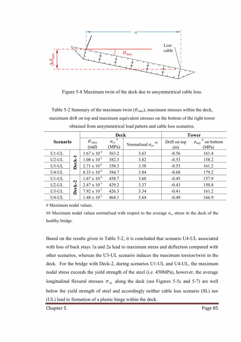
Chapter 5 Page 85

Figure 5-8 Maximum twist of the deck due to unsymmetrical cable loss.

Table 5-2 Summary of the maximum twist ( max), maximum stresses within the deck,

maximum drift on top and maximum equivalent stresses on the bottom of the right tower

obtained from unsymmetrical load pattern and cable loss scenarios.

Scenario

Deck Tower max

(rad) σxx

# (MPa) Normalised σxx

## Drift on top (m)

σeqv # on bottom (MPa)

U1-UL

Dec

k-1 1.67 x 10-4 363.2 3.63 -0.56 161.4

U2-UL 1.08 x 10-3 382.3 3.82 -0.53 158.2 U3-UL 2.71 x 10-2 358.3 3.58 -0.53 161.2 U4-UL 8.33 x 10-4 384.7 3.84 -0.68 179.2 U1-UL

Dec

k-2 1.67 x 10-4 458.7 3.60 -0.45 157.9

U2-UL 2.47 x 10-3 429.2 3.37 -0.43 150.8 U3-UL 7.92 x 10-2 426.3 3.34 -0.41 161.2 U4-UL 1.48 x 10-2 464.1 3.64 -0.49 166.9

# Maximum nodal values.

## Maximum nodal values normalised with respect to the average σxx stress in the deck of the

healthy bridge.

Based on the results given in Table 5-2, it is concluded that scenario U4-UL associated

with loss of back stays 1a and 2a lead to maximum stress and deflection compared with

other scenarios, whereas the U3-UL scenario induces the maximum torsion/twist in the

deck. For the bridge with Deck-2, during scenarios U1-UL and U4-UL, the maximum

nodal stress exceeds the yield strength of the steel (i.e. 450MPa), however, the average

longitudinal flexural stresses xx along the deck (see Figures 5-5c and 5-7) are well

below the yield strength of steel and accordingly neither cable loss scenario (SL) nor

(UL) lead to formation of a plastic hinge within the deck.

max max

w

Lost cable

Chapter 5 Page 86

Overall, the stresses induced in the bridges with Deck-1 and Deck-2 during

unsymmetrical cable loss scenarios have the same magnitude. In order to further assess

the effect of deck configuration on the potential progressive collapse response during

different cable loss scenarios, the maximum stress induced in Deck-1 and Deck-2 are

normalised with respect to the maximum stress occurred in the healthy bridge and the

values are reported in Table 5-2 that demonstrate the minor influence of the deck

configuration on the response of the deck following different cable loss scenarios.

5.4.3 Cables

Envelop of maximum and minimum tensile stresses in the cables for symmetrical (SL)

scenarios are shown in Figures 5-9a and 5-9b, respectively. It is seen that the axial

stress in the cables is well below the breakage stress ( MPa1860u ) of the cables. In

addition, the minimum axial stresses in the cables are used for calculating the minimum

equivalent modulus of elasticity E (Ernst’s modulus) of cables which are shown in

Figure 5-9c. It is seen that for the longest cables connected to the mid-span EE 94.0

which would have a minor influence on the response of the bridge.

Envelops of the maximum tensile stress in the cables “a” and “b” (see Figure 5-1)

during unsymmetrical (UL) scenarios are shown in Figures 5-10 and 5-11, respectively.

It is observed that the axial stress in the cables for the considered unsymmetrical cable

loss scenarios is well below the breakage stress ( MPa1860u ) of the cables and

accordingly in the cable stayed bridge under consideration, no zipper-type progressive

collapse is expected to occur due to symmetrical or unsymmetrical loss of two cables.

In addition, the minimum equivalent modulus of elasticity E (Ernst’s modulus of

cables) expressed as a ratio of modulus of elasticity E during unsymmetrical (UL)

scenarios for Deck-1 and Deck-2 are shown in Figure 5-12. It is seen that for the bridge

with Deck-2 subjected to unsymmetrical (U4-UL) scenario, the minimum E is as low as

E88.0 for cable 30 (see Figure 5-12d) that can affect the dynamic response and

accordingly should not be ignored in the progressive collapse assessment of the bridge.

Chapter 5 Page 87

(a)

(b)

(c)

Figure 5-9 Envelop of the (a) maximum tensile stress over ultimate strength (b)

minimum tensile stress over ultimate strength and (c) the minimum equivalent modulus

of elasticity E (Ernst’s modulus of cables) expressed as a percentage of modulus of

elasticity E in the cables during symmetrical (SL) cable loss and loading scenarios.

20%

30%

40%

50%

60%

70%

0 10 20 30 40 50 60

Cab

le st

ress

rat

io

Cable no.

Deck-1Deck-2

20%

30%

40%

50%

60%

0 10 20 30 40 50 60

Cab

le st

ress

rat

io

Cable no.

Deck-1Deck-2

0.92

0.94

0.96

0.98

1.00

0 10 20 30 40 50 60

E/E

rat

io

Deck-1Deck-2

Cable no.

Chapter 5 Page 88

(a) U1-UL

(b) U2-UL

(c) U3-UL

(d) U4-UL

Figure 5-10 Envelop of the maximum tensile stress in cables “a” (z=9.6) during

unsymmetrical (UL) scenarios.

20%

30%

40%

50%

60%

0 10 20 30 40 50 60

Cab

le st

ress

rat

io

Cable no.

Deck-1Deck-2

20%

30%

40%

50%

60%

0 10 20 30 40 50 60

Cab

le st

ress

rat

io

Cable no.

Deck-1Deck-2

20%

30%

40%

50%

60%

0 10 20 30 40 50 60

Cab

le st

ress

rat

io

Cable no.

Deck-1Deck-2

20%

30%

40%

50%

60%

0 10 20 30 40 50 60

Cab

le st

ress

rat

io

Cable no.

Deck-1Deck-2

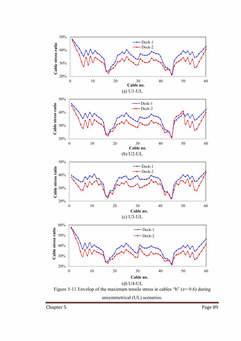
Chapter 5 Page 89

(a) U1-UL

(b) U2-UL

(c) U3-UL

(d) U4-UL

Figure 5-11 Envelop of the maximum tensile stress in cables “b” (z=-9.6) during

unsymmetrical (UL) scenarios.

20%

30%

40%

50%

0 10 20 30 40 50 60

Cab

le st

ress

rat

io

Cable no.

Deck-1Deck-2

20%

30%

40%

50%

0 10 20 30 40 50 60

Cab

le st

ress

rat

io

Cable no.

Deck-1Deck-2

20%

30%

40%

50%

0 10 20 30 40 50 60

Cab

le st

ress

rat

io

Cable no.

Deck-1Deck-2

20%

30%

40%

50%

60%

0 10 20 30 40 50 60

Cab

le st

ress

rat

io

Cable no.

Deck-1Deck-2

Chapter 5 Page 90

(a) Cables “a” (z=9.6) –Deck1

(b) Cables “b” (z=-9.6) –Deck1

(c) Cables “a” (z=9.6) –Deck2

(d) Cables “b” (z=-9.6) –Deck2

Figure 5-12 The minimum equivalent modulus of elasticity E (Ernst’s modulus of

cables) expressed as a ratio of modulus of elasticity E during unsymmetrical (UL)

scenarios.

0.94

0.96

0.98

1.00

0 10 20 30 40 50 60

E/E

rat

io

Cable no.

U1U2U3U4

0.92

0.94

0.96

0.98

1.00

0 10 20 30 40 50 60

E/E

rat

io

Cable no.

U1U2U3U4

0.92

0.94

0.96

0.98

1.00

0 10 20 30 40 50 60

E/E

rat

io

Cable no.

U1U2U3U4

0.880.900.920.940.960.981.00

0 10 20 30 40 50 60

E/E

rat

io

Cable no.

U1U2U3U4

Chapter 5 Page 91

5.4.4 Sensitivity Analysis

With regard to the variability in strength and stiffness of materials, a sensitivity analysis

is carried out to demonstrate the robustness of the FE results and also evaluate the

influence of mechanical properties of steel (i.e. yield strength y and elastic modulus E

) on the potential progressive collapse response of the cable stayed bridge. The scenario

U4-UL (loss of cables No. 1a and 2a) that led to maximum vertical deflection and

maximum stresses in the structural components (i.e. deck and cables) and ±10%

variability in the steel modulus of elasticity E is considered in this sensitivity analysis.

The sensitivity of deflection response (along the deck) with respect to the yield strength

y and elastic modulus E of the steel during scenario U4-UL is shown in Figure 5-13.

(a) Deck-1

(b) Deck-2

Figure 5-13 Sensitivity of the deflected configuration of the deck (when maximum

vertical displacement has occurred in scenario U4-UL) with respect to steel yield

strength y and elastic modulus E .

-2.0

-1.5

-1.0

-0.5

0.0

0.5

1.0

0 100 200 300 400 500 600 700 800 900 1000

σy=450 MPa E=200 GPa σy=400 MPa E=200 GPa σy=400 MPa E=180 GPa σy=400 MPa E=220 GPa

-2.0

-1.5

-1.0

-0.5

0.0

0.5

1.0

1.5

0 100 200 300 400 500 600 700 800 900 1000

σy=450MPa E=200GPa σy=400MPa E=200GPa σy=400MPa E=180GPa σy=400MPa E=220GPa

Ver

tical

def

lect

ion

(m)

Coordinate along the deck (m)

Ver

tical

def

lect

ion

(m)

Coordinate along the deck (m)

Max. Sagging

Max. Sagging

Max. Hogging

Max. Hogging

Chapter 5 Page 92

(a) Deck-1

(b) Deck-2

Figure 5-14 Sensitivity of average xx stress component on top surface of the deck

(when maximum vertical displacement has occurred in scenario U4-UL) with respect to

steel yield strength y and elastic modulus E .

In addition, the sensitivity of average xx stress component on top surface of the deck

(when maximum vertical displacement has occurred) with respect to the yield strength

and elastic modulus of the steel during scenario U4-UL is shown in Figure 5-14. It is

observable that the variation of response (i.e. vertical deflection and xx stress) is within

the range of variability assumed for mechanical properties of steel.

With regard to the results shown in Figures 5-13 and 5-14, it is seen that the deflected

configuration of the deck (locations of maximum sagging and hogging deflection) and

the variation of xx stress along the deck (locations of maximum xx ) are not sensitive

to the yield strength and elastic modulus of steel. This is clearly demonstrative of the

robustness as well as adequacy of the results obtained from the FE models.

-150

-100

-50

0

50

100

150

0 100 200 300 400 500 600 700 800 900 1000

σy=450 MPa E=200 GPa σy=400 MPa E=200 GPa σy=400 MPa E=180 GPa σy=400 MPa E=220 GPa

-150

-100

-50

0

50

100

150

0 100 200 300 400 500 600 700 800 900 1000

σy=450 MPa E=200 GPa σy=400 MPa E=180 GPa σy=400 MPa E=200 GPa σy=400 MPa E=220 GPa

xx to

p of

dec

k (M

Pa)

xx to

p of

dec

k (M

Pa)

Coordinate along the deck (m)

Coordinate along the deck (m)

Max. xx

Max. xx

Chapter 5 Page 93

5.5 Conclusions and Discussion

A detailed nonlinear 3D finite element model of a cable-stayed bridge with two

different configurations of deck (i.e. steel box girder vs open orthotropic girder) was

developed in this chapter. The results of 3D FE model, including axial stress on top

surface of the deck, deflected profile of the deck, and tensile stress in cables, are

compared with corresponding 2D FE models and validated. The developed 3D FE

model was used for progressive collapse assessment of the bridge subjected to

symmetrical and unsymmetrical cable loss scenarios with lost cables at different

locations. Especially, the scenarios associated with loss of two back stays connected

around the supports were studied in more details. With regards to the parametric studies

undertaken in this chapter, the following conclusions for the cable stayed bridge under

consideration can be drawn;

- The configuration of the deck (e.g. box girder or orthotropic open girder) as well

as the torsional stiffness of the deck was found to have minor influence on the

potential collapse response of the cable stayed bridge following loss of one or

two cables.

- The cable loss scenarios associated with loss of back stays (cable 1a and 2) were

the most critical scenarios that lead to maximum stress and deflection compared

with other scenarios. This observation is consistent with the results obtained

from detailed linear elastic 3D FE models (Aoki et al., 2012b).

- The stresses induced in the deck by the torsional mode of vibration were shown

to have minor influence on the response of the bridge (no buckling or yielding of

steel was observed). Also, a sensitivity analysis was carried out and it was

shown that the yield strength of steel has no influence on the potential

progressive collapse response of the cable stayed bridge investigated in this

paper.

- The tensile stress in the stays following the cable loss scenarios remained well

below the breakage stress of the cables and accordingly for the cable stayed

bridge considered in this paper, loss of one or even two cables cannot trigger a

zipper-type progressive collapse.

Chapter 5 Page 94

- The change in shape (geometry) and the reduction in axial stiffness of the stays

due to variation of stress levels in the cables were evaluated with respect to

Ernst’s modulus. The variation of Ernst’s modulus in the longest stays was

found to be less than 12% and this is demonstrative of the magnitude of

geometrical nonlinearities in the cables during progressive collapse assessment

of the cable stayed bridges.

- In the analysed bridge, material nonlinearity (yielding of steel) and buckling of

steel plates did not occur at global as well as local levels. Accordingly, it was

concluded that the zipper-type collapse triggered by formation of plastic hinges

is unlikely to happen in the cable stayed bridges that have lost two cables or less.

Chapter 6 Page 95

: Cable-Stayed Bridges and Blast Chapter 6

Loads Summary of chapter

One of the reasons for loss of cable(s) in cable –stayed bridges can be blast loading that

has become a major concern after the 911 terrorist attacks. In this chapter, a detailed

nonlinear 3D finite element model is used to simulate the effect of blast loadings with

different amounts of explosives at different locations along the deck, to determine the

number of potential cable losses due to explosion. Moreover, the results obtained from

the direct cable loss analyses due to blast loadings are compared with simple cable loss

scenarios (presented in previous Chapters 3 to 5) according to alternate load path (ALP)

approach. Finally, the potential of the progressive collapse of the bridge at global and

local levels is investigated. With regard to the results of FE analyses, it is concluded

that up to a maximum of three stays could be lost if a large enough TNT equivalent

charge is detonated in the critical region around the end supports. However, loss of

three cables with damage to the anchorage zone area within the end support did not

trigger the progressive collapse of the entire bridge. It is shown that the simple cable

loss analysis based on ALP can adequately capture the response (i.e. deformation along

the deck and tower, and maximum stress levels in the regions sufficiently away from

the explosion) of the cable stayed bridge following cable loss due to direct blast load.

The short cables near the tower are identified as the most sensitive cables in which the

stress level is significantly influenced by the blast loadings. However, these short cables

are not sensitively influenced by the simple cable loss analysis.

6.1 Introduction

In previous 3 chapters (Chapters 3 to 5), the effect of loss of cable(s) were studied by

using alternate load path (ALP) method. Linear as well as nonlinear dynamic analyses

following different cable loss scenarios were conducted and dynamic amplification

factor (DAF) for different structural components were determined.

Chapter 6 Page 96

A wide range of loading scenarios such as corrosion, collision of vehicles, earthquake

and blast can lead to cable loss and subsequently catastrophic progressive collapse of

the entire bridge. Among different extreme loading scenarios, however, the loss of

cables due to air blast and explosion has become a major concern since 911 terrorist

attacks.

The progressive collapse assessment of structures prone to terrorist attacks can be

carried out by directly simulating the explosion or alternatively applying the air blast

pressure on the structure and obtaining the structural response (Shi et al., 2010). This

approach is accurate, however, it is computationally demanding. On the other hand,

there are simplified progressive collapse analysis methods based on alternate load path

(ALP) approach, in which, the load carrying structural components such as columns

and/or cables are removed in some hypothetical scenarios to simulate the implications

of critical member loss due to blast loadings. However, some researchers claim that the

simplified method based on ALP cannot adequately predict the progressive collapse

response of the structure subject to blast loading (Shi et al., 2010).

Therefore, in this research, these two methods will be applied to a cable-stayed bridge

and compared to determine the accuracy of simplified method since many research

works have been conducted using the simplified method.

In this study, nonlinear 3D FE models of a cable stayed bridge is developed using LS-

DYNA (2007) and ANSYS software (2009). The developed FE models can take

account of material and geometrical non-linearity including large strains and

displacements. Using the developed 3D FE model in LS-DYNA, blast load analysis was

carried out to determine the air blast pressure. Then, the air blast pressure is

automatically applied on the bridge to determine the extent of the damage in the deck as

well as the lost (fully damaged) cable(s). Furthermore, the dynamic response of the

bridge following loss of fully damaged cables is captured by the LS-DYNA model and

the results are compared with the FE model predictions in which the ALP method is

used to assess the potential progressive collapse response of the bridge following cable

loss due to explosion.

Chapter 6 Page 97

6.2 Adopted assumptions

6.2.1 Geometry, material properties and design loads

The adopted assumptions including bridge configuration, material properties, 3D FE

model used in conjunction with ALP method and design loads in this chapter are as

given in Chapter 4, Sections 4.2 and 4.3.

6.2.2 Modelling and analysis

Similar to previous chapters, the developed FE models can take account of large

displacements and geometrical nonlinearities. Furthermore, for dynamic analysis a

proportional damping with mass and stiffness multipliers of 0.5% is adopted,

which is within the acceptable range for steel structures (Clough and Penzien, 1993).

(a) Explicit model (LS-DYNA)

(b) Implicit model (ANSYS)

Figure 6-1 Outline of the 3D finite element models.

Chapter 6 Page 98

In this chapter, the bridge model was developed using both LS-DYNA and ANSYS

software (see Figure 6-1). The LS-DYNA model with an explicit solver was employed

for blast analysis and capturing the local/global response of the bridge subject to air

blast pressure, whereas the ANSYS model with an implicit solver was used to capture

the local/global response of the bridge following sudden loss of cable(s) based on ALP

approach.

In LS-DYNA 3D model (Figure 6-1a), the deck and tower are modelled by shell

element (Belytschko-Tsay element formulation). This shell element is defined by 8

nodes with 6-dofs at each node and it takes advantage of a reduced integration scheme

with 2 integration points over the thickness of the element. The material model used in

conjunction with this shell element to capture the nonlinear behaviour of steel plates is

material number 24 which is MAT_PIECEWISE_LINEAR_PLASTICITY. This is an

elasto-plastic material for which failure mode based on plastic strain can be defined by a

bilinear stress strain curve. In this research, steel plastic strain failure value was set as

0.06 (see Figure 4-2 in Chapter 4). When the plastic strain within an element reaches

this value, the element is removed from the numerical model. Moreover, cables in LS-

DYNA were modelled by discrete beam/cable elements with 2 Gauss points. The

material type 71 called MAT_CABLE_DISCRETE_BEAM was used for modelling

cables. This beam element can model an elastic cable without compressive force

(tensile only). This beam/cable element also has the ability to take account of the cable

pre-tensioning force at the start of the analysis. The initial pre-tensioning strains

induced in the cables were given in Table 4-1 in chapter 4.

The 3D FE model developed in ANSYS (Figure 6-1b) is analysed using an implicit

solver. In ANSYS, the deck and towers are modelled by shell elements, whereas the

cables are modelled by link-elements which are treated as tension-only members with

limited tensile capacity. More details on the element type and material constitutive laws

adopted in ANSYS model were provided in Section 4.2.2 of Chapter 4.

Explicit versus implicit analysis

Typically direct step-by-step integration schemes are used for time discretisation of

differential equations governing dynamic response of structures (Cook et al., 2002),

Chapter 6 Page 99

extnn n n

M D C D K D R (6-1)

where, M , C and K are mass, damping and stiffness matrix of the structure,

respectively. n

Dn

D , n

Dn

D and nD denote current nodal acceleration, velocity and

displacement vectors and ext

nR is the current vector of external dynamic load.

A wide range of time discretisation techniques for solving Equation (6-1) have been

proposed to date. These time discretisation methods mostly take advantage of finite

difference schemes and accordingly they are categorised to explicit and implicit

methods (Cook et al., 2002). In the explicit schemes the unknown displacement vector

1nD is an explicit function of acceleration, velocity and displacement vectors of

previous steps

1 1, , , ,...

n n nn nD f D D D DD D D, ,, , (6-2)

whereas in an implicit solution scheme

1 1 1, , , , ,...

n nn n n nD f D D D D D ,...

n1 1 n nn1D D D D D

1, , , ,, , ,

1 n1 1,

111 (6-3)

Accordingly, implicit methods should use iterative schemes for capturing nonlinear

behaviour of structures. The major differences between explicit and implicit methods

are stability and economy. The time step is a critical factor in both methods, however,

the required time step for explicit solvers is much smaller than the implicit schemes.

The explicit solvers need to use a large number of time steps, but the process involves

solving the simultaneous set of governing equations is very fast because the coefficient

matrix of 1nD can be made diagonal. On the other hand, in implicit methods the

number of time steps is fairly small, but at each step a few iterations are required to

adequately satisfy the equilibrium and compatibility conditions (Cook et al., 2002).

In summary, explicit schemes are appropriate for wave propagation problems including

blast or impact loadings, whereas implicit schemes are suitable for structural dynamics

problem such as analysis of structures subject to seismic actions.

Chapter 6 Page 100

6.2.3 Verification and calibration of LS-DYNA model (Explicit Solver)

In this section, the results obtained from the LS-DYNA model with an explicit solver is

compared with the results predicted by ANSYS model that takes advantage of an

implicit solver. The main objective is to calibrate the explicit solver and verify its

adequacy compared with the more reliable implicit solver. The cable initial force over

the cable breakage load and xx stress on top surface of the healthy bridge deck

predicted by LS-DYNA, ANSYS and 2D FE models are compared in Figure 6-2 that

demonstrates a good correlation among the three sets of FE models. Furthermore, the

total weight of the bridge obtained from 2D, 3D-implicit and 3D-explicit FE models

under progressive collapse load combination of (1.1xDead+1.35xSuperimposed

Dead+0.75xTraffic) are 647 MN, 656 MN and 641MN, respectively.

(a)

(b)

Figure 6-2 Comparison between results of 2D, implicit (ANSYS) and explicit (LS-

DYNA) 3D FE models (a) ratio of axial force (stress) over breakage load (stress) for

stays (under service load) (b) xx stress component on top surface of the deck.

20%

30%

40%

50%

0 10 20 30 40 50 60

Cab

le st

ress

rat

io (%

)

Cable no.

LS-DYNAANSYS2D

-150

-100

-50

0

50

100

0 100 200 300 400 500 600 700 800 900 1000

σ xx s

tres

s (M

Pa)

LS-DYNAANSYS2D Model

Chapter 6 Page 101

6.3 Blast load analysis and sudden loss of cable

6.3.1 Blast load analysis by explicit analysis (LS-DYNA)

The blast load analysis adopted in this study is purely based on Lagrangian approach, in

which the surface of the shell elements (set by *SET_SEGMENT) is defined to receive

the blast load pressure calculated according to CONWEP blast function. The code used

for this method is *LOAD_BLAST_ENHANCED (Tabatabaei and Volz, 2012). By

using this code, pressure loads caused by the explosion of conventional charge is

defined as an air blast function that include treatment of reflected waves, moving

warheads and multiple blast sources (LSTC, 2007).

To verify adequacy of the adopted blast load analysis method, a simple numerical steel

column subjected to a direct air blast loading scenario was modelled by LS-DYNA and

the LS-DYNA prediction was compared with other numerical results as well as the

available experimental data.

The steel column considered in this verification study is 4.3 m in height, 0.36 m in

width and 0.122 m in depth and made of Grade 345 steel. This steel column was

originally tested by Lawver et al. (2003). Furthermore, McConnell and Brown (2011)

developed a FE model of this column in LS-DYNA software using shell elements (same

element formulation) and with *MAT_JOHNSON_COOK material model. The

schematic outline of the FE develop by McConnell and Brown (2011) is shown in

Figure 6-3a. As McConnell and Brown mentioned in their paper, Lawver’s

experimental work was insufficiently presented in their paper due to confidentiality of

the experimental data. Accordingly, McConnell and Brown had to assume some of the

input data such as the amount of TNT charge and the scaled distance. With regard to the

data provided by McConnell and Brown (2011) and Lawver et al. (2003), the

equivalent TNT charge and scaled distance were taken as 1,000 kg and 2.1 m,

respectively.

The maximum horizontal deflection at different height along the column obtained from

the LS-DYNA model in this study is shown in Figure 6-3b along with predicted by

McConnell and Brown’s (2011) FE model predictions and Lawver’s experimental data.

Chapter 6 Page 102

(a) FEA model (McConnell and Brown, 2011)

(b) Displacement

Figure 6-3 Comparison of validation model with other references

It is seen that the results of LS-DYNA model developed in this study correlates

reasonably well with the test data. The maximum difference between the FE models is

around 25%, however, the difference between maximum deflection predicted by the

LS-DYNA FE model and the experimental results is less than 10%. This example

demonstrates the adequacy of LS-DYNA FE models and explicit solvers for capturing

the local and global response of structural members subjected to direct blast load.

0

1

2

3

4

5

0 2 4 6 8 10

Hei

ght (

m)

Displacement (cm)

Lawver et al ExperimentalLawver et al FixedLawver et al PinnedMacConnell and BrownPresent study

Chapter 6 Page 103

6.3.2 Load combinations adopted for blast and sudden loss of cable analyses

For blast loading analysis, the distributed component of the traffic load, the dead load,

and the accompanying lane factor from Australian standard AS5100.2 (2004) was

applied along the entire bridge deck, which is the same as symmetrical loading pattern

considered in Chapter 5 and shown in Figure 5-2a and b. The adopted load factors are

as recommended by AASHTO LRFD bridge design specification reported in NCHRP

(2003)

1.00 0.5 1.0DC LL EV (6-4)

where, DC denotes the dead load of the structural components and non-structural

attachments, LL is the full vehicular live load placed in the actual stripped lanes, and EV

denotes extreme event load, which is the blast load in this chapter.

6.3.3 Scenario considered for Blast load analysis

In this chapter, three different charges of TNT are considered for blast load analysis,

i.e. 1 tonne, 4.5 tonnes and 27 tonnes. The 1 tonne TNT equivalent explosive was

adopted as the smallest possible charge for blast assessment of the bridge in accordance

with a study undertaken by Hao and Tang (2010). The 4.5 and 27 tonnes TNT

equivalent explosives are considered in this study as the maximum capacity of a small

box van and a semi-trailer, respectively (Mahoney, 2007).

In the adopted blast analysis model of LS-DYNA, the contact surface has to be defined

for applying the air blast pressure on the structure. Accordingly, a sensitivity analysis

was carried out and the area of contact surface for blast loading was set as 25.6 m ×

40 m and the detonation centre was placed at the middle of this contact surface. Within

this contact surface, the element size is taken as 1/3 of the other part of the structure

(approximately 0.25 m × 0.25 m elements). The cable element (link element) was too

small to be subjected to the direct air blast pressure, thus, it was not defined as a contact

surface.

There are eight locations where the blast load was applied (see Figure 6-4a and 6-4b);

three locations near the pin-support (x=2.5, 5.0 and 7.5 m), two locations near the tower

(x=225 and 235 m) and three locations around the mid-span (x=515, 525 and 535 m).

Chapter 6 Page 104

As shown in Figure 6-4c, the blast charge (detonation centre) was located at different

heights depending on the scaled distance obtained from the following equation,

13

RZW

(6-5)

where Z is the scaled distance (in m/kg1/3), R is the distance between contact surface and

the detonation centre and W is the equivalent TNT amount.

(a) Blast load location (x-distance from pin support [A-A])

(b) Blast load location (x-distance from pin support)

(c) Blast load location (y- and z-distances)

Figure 6-4 Locations of the applied blast loadings.

x

y

x

y

z y

x=515m

Chapter 6 Page 105

It is noteworthy that the CONWEP blast pressure function used in LS-DYNA for blast

analysis is not applicable for very close range explosions and hence the scaled distance

cannot be taken too small. In this study, Z is set equal to 0.1 and the R value is back

calculated with respect to the amount of TNT equivalent explosive and based on

Equation (6-5).

The cables are closely-spaced around the pin-support and these cables were found to be

the most critical in terms of producing possible potential progressive collapse of the

entire bridge (see in Chapter 3). Accordingly, three different sets of blast scenario with

different amount of TNT equivalent explosive were considered assuming that

explosions occur in the vicinity of pin-support. The TNT charge was placed in different

locations to investigate the extent of damaged area and number of potential cable losses

(total of 9 scenarios, i.e. Scenario: 1t_2.5m to Scenario: 27t_7.5m shown in Table 6-1).

Apart from the blast scenarios around the pin-support, the 27-tonne TNT equivalent

charge was placed at a location close to tower and mid-span (Scenario: 27t_515m to

Scenario: 27t_235m). The list of considered blast scenarios along with the locations and

amount of TNT equivalent explosive charges in each scenario are provided in Table 6-1

and Figure 6-4.

Table 6-1 Scenarios considered for blast load analysis (using LS-DYNA software).

Scenario Equivalent TNT (Tonnes)

Distance from pin-support (m)

scaled distance – Z (m/kg1/3)

Bla

st lo

ad a

naly

sis

Scenario:1t_2.5m 1

2.5

0.1

Scenario:1t_5.0m 5 Scenario:1t_7.5m 7.5

Scenario:4.5t_2.5m 4.5

2.5 Scenario:4.5t_5.0m 5 Scenario:4.5t_7.5m 7.5 Scenario:27t_2.5m

27

2.5 Scenario:27t_5.0m 5 Scenario:27t_7.5m 7.5 Scenario:27t_515m 515 Scenario:27t_525m 525 Scenario:27t_535m 535 Scenario:27t_225m 225 Scenario:27t_235m 235

Chapter 6 Page 106

6.3.4 Analysis of sudden cable loss using ALP approach and implicit solver

(ANSYS)

A parametric study of cable losses by dynamic analysis using ANSYS software was

presented in previous chapters. The EKILL command, available in ANSYS (2009) was

used to remove the damaged cables and simulate the implications of possible cable

losses due to blast load. In this chapter, the cable loss analysis using Ekill command

(which is called hereafter “simple cable loss analysis”) is compared with the FE

simulations including the blast load analysis (i.e. LS-DYNA model). One cable loss (1a,

2a, 15a and 30a), two cable losses (1a and 2a) and three cable losses (1a to 3a) are

considered as summarised in Table 6-2.

Table 6-2 Scenarios considered - equivalent cable loss analysis (simple cable loss

analysis) -implicit analysis by ANSYS

Scenarios cable loss

Equ

ival

ent c

able

loss

ana

lysi

s

Scenario: 1a loss-ANSYS 1a Scenario: 2a loss-ANSYS 2a Scenario: 1a & 2a loss-ANSYS 1a & 2a Scenario: 1a,2a & 3a loss-ANSYS 1a, 2a & 3a Scenario: 30a loss-ANSYS 30a Scenario: 15a loss-ANSYS 15a

6.4 Results and discussion

6.4.1 Results of blast analysis (LS-DYNA)

The damaged area due to blast around the pin-support predicted by LS-DYNA model is

shown in Figure 6-5. Furthermore, Table 6-3 summarises the damaged area and the

corresponding loss of cables. In Figure 6-5a to 6-5c, the damaged area due to 1 tonne of

TNT was about 4.8 m × 3.6 m with no cable losses. The most significant damage area

and cable loss was created by 27 tonnes of TNT located at x=5.0 m (beside cable 2a)

and 7.5 m (between cables 2a and 3a) and both scenarios led to loss of three cables.

It is noted that the damaged area is almost square shaped (straight lines). This is because

of the stiffener plates used horizontally every 2.5 m apart along the whole bridge deck.

The 27 tonnes of TNT equivalent charge damaged an area of 11 m × 11 m and if there

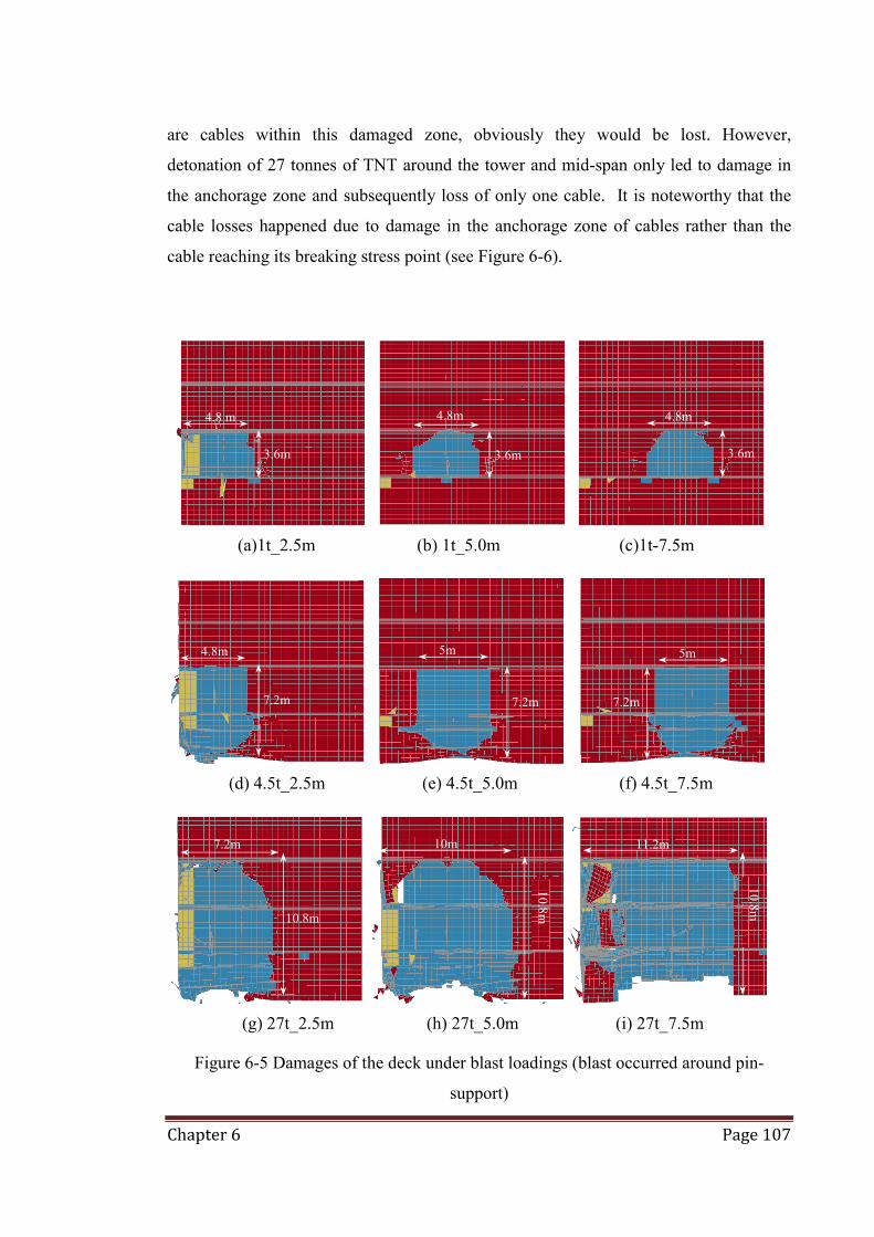
Chapter 6 Page 107

are cables within this damaged zone, obviously they would be lost. However,

detonation of 27 tonnes of TNT around the tower and mid-span only led to damage in

the anchorage zone and subsequently loss of only one cable. It is noteworthy that the

cable losses happened due to damage in the anchorage zone of cables rather than the

cable reaching its breaking stress point (see Figure 6-6).

(a)1t_2.5m (b) 1t_5.0m (c)1t-7.5m

(d) 4.5t_2.5m (e) 4.5t_5.0m (f) 4.5t_7.5m

(g) 27t_2.5m (h) 27t_5.0m (i) 27t_7.5m

Figure 6-5 Damages of the deck under blast loadings (blast occurred around pin-

support)

7.2m

10.8m

10m

10.8m

4.8m

7.2m

5m

7.2m

5m

7.2m

3.6m

4.8m

3.6m

4.8m

3.6m

11.2m

10.8m

4.8 m

Chapter 6 Page 108

Table 6-3 Summary of the cable losses and damaged areas obtained from blast load

analysis.

Cable loss Damaged area A

roun

d pi

n-su

ppor

t Scenario:1t_2.5m

None 4.8m x 3.6m Scenario:1t_5.0m Scenario:1t_7.5m

Scenario:4.5t_2.5m cable 1a 4.8m x 7.2m Scenario:4.5t_5.0m cable 2a

5.0m x 7.2m Scenario:4.5t_7.5m None Scenario:27t_2.5m cable 1a & 2a 7.2m x 10.8m Scenario:27t_5.0m Cable 1a, 2a & 3a 10m x 10.8m Scenario:27t_7.5m Cable 1a, 2a & 3a 11.2m x 10.8m

Mid-span Scenario:27t_515m None

11.2m x 10.8m Scenario:27t_525m Cable 30a Scenario:27t_535m None

Beside the tower

Scenario:27t_225m Cable 15a 10m x 10.8m Scenario:27t_235m None

Figure 6-6 Time history of stress (expressed as a percentage of breakage stress) for

cables No.1a and 1b (Scenario: 27t_7.5m).

0%

10%

20%

30%

40%

50%

60%

0 5 10 15 20 25 30

Cab

le st

ress

rat

io

Time (sec)

cable no.cable1a

cable no.cable1b

Chapter 6 Page 109

6.4.2 Comparative study between blast load and simple cable loss according to

ALP (blast around the pin support)

In this section, the effect of blast load impact and the local damage caused by air blast is

investigated. Furthermore, the response of the bridge subjected to direct blast load and

subsequent cable loss is compared with the response captured by simple cable loss

analysis based on alternate load path (ALP) method to verify the adequacy of widely

accepted ALP method. It should be noted that the blast load analysis provides

information on cable loss as well as local damages, whereas the ALP method can only

capture the structural implications of cable loss due to explosion.

With regard to the lost cables following blast scenarios around pin-support (see Table 6-

3), Scenario: 4.5t_2.5m is compared with 1a_loss _ANSYS, and Scenario: 4.5t_5m is

compared with 2a_loss_ANSYS, Scenario: 27t_2.5m is then compared with 1a &

2a_loss _ANSYS, and finally Scenario: 27t_5m and 27t-7.5m are compared with 1a to

3a_loss _ANSYS, respectively.

Deck and Tower

The magnitude of maximum vertical deflection within the deck, profile of the maximum

σxx (longitudinal stress) on top and bottom surface of the deck, and maximum lateral

drift on top and maximum equivalent stress σeqv at the bottom of the right tower

obtained from blast analysis and simple cable loss analysis are compared in Table 6-4.

In addition, deflected configurations of the deck when maximum vertical displacement

has occurred for each scenario are shown in Figure 6-7. It is observed that the

deflections are predicted quite well in all cases. The average difference between the

ALP and direct blast analysis is around 21% to 23%.

The average xx stress component on the surface of the top and bottom of the deck

(when maximum stress has occurred) for all scenarios are shown in Figures 6-8 and 6-9,

respectively. The difference between xx stress component predicted by ALP and direct

blast analysis is around 7% and 11% for the top and about 17% for the bottom surface

of the deck. With regard to the results given in Table 6-4, during scenarios 27t_2.5m

and 27t_7.5m the maximum nodal stress σxx exceeds the yield strength of the steel (i.e.

Chapter 6 Page 110

450MPa), however, the average longitudinal flexural stresses σxx along the deck (see

Figures 6-9c and 6-9d) are well below the yield strength of steel and accordingly neither

blast analysis nor ALP cable loss analysis showed formation of any plastic hinges

within the deck. Moreover, both analyses affected the tower drift and maximum

equivalent stress σeqv at the bottom insignificantly, even with blast is occurring near the

tower.

Cables

Comparison of cable stresses captured by two different methods, i.e. ALP and direct

blast analysis is carried out for cables on left and right side of the deck. The cable stress

envelops are shown in Figure 6-10 (side-a where blast occurred, see Figure 6-4c) and

Figure 6-11 (side-b), respectively. It is observed that no cable exceeded the breakage

stress and the maximum stress ratio was about 57% during Scenario: 27t_5m. In cables

10-20 and 40-50, the stresses obtained from the direct blast analysis are considerably

higher than the results predicted by the ALP cable loss analysis. It can be concluded that

the stress in these short cables is sensitive to the adopted choice of analysis.

Table 6-4 Summary of maximum deflection, stresses for deck and tower obtained from

explicit analysis (blast loading analysis) and implicit analysis (loss of cable analysis)

Deck Tower Cable

loss Scenarios δy-max σxx-top σxx-bot δx-max σeqv

1a Scenario:4.5t_2.5m -0.769 362.4 446.4 0.407 128.76 Scenario: 1a loss-ANSYS -0.876 323.2 337.4 0.438 119.68

2a Scenario:4.5t_5.0m -0.695 419.2 334.3 0.396 125.86 Scenario: 2a loss-ANSYS -0.783 321.3 332.2 0.417 116.29

1a & 2a

Scenario:27t_2.5m -1.240 346.0 453.6 0.492 146.19 Scenario: 1a&2a loss-ANSYS -1.381 349.1 363.3 0.533 135.41

1a, 2a &

3a

Scenario:27t_5.0m -1.730 392.7 411.4 0.646 153.87 Scenario:27t_7.5m -1.770 419.3 459.2 0.656 153.88 Scenario: 1a, 2a&3a loss-ANSYS -1.902 379.1 365.6 0.654 148.95

30a Scenario:27t_525m -0.589 277.6 313.1 0.371 124.60 Scenario: 30a loss-ANSYS -0.756 305.0 290.7 0.414 125.35

15a Scenario:27t_225m 0.389 337.1 352.6 0.371 124.60 Scenario: 15a loss-ANSYS -0.473 297.2 273.4 0.349 104.95

Chapter 6 Page 111

(a) 1 cable loss (1a)

(b) 1 cable loss (2a)

(c) 2 cable loss (1a and 2a)

(d) 3 cable loss (1a-3a)

Figure 6-7 vertical displacements along the deck for scenarios with 1, 2 and 3 cable

losses.

-1.5

-1.0

-0.5

0.0

0.5

1.0

0 100 200 300 400 500 600 700 800 900 1000

Ver

tical

def

lect

ion

(m)

1a loss-ANSYS4.5t-2.5m

-1

-0.5

0

0.5

0 100 200 300 400 500 600 700 800 900 1000

Ver

tical

def

lect

ion

(m) 2a loss-ANSYS

4.5t-5m

-1.5

-1

-0.5

0

0.5

1

0 100 200 300 400 500 600 700 800 900 1000

Ver

tical

def

lect

ion

(m)

1a&2a loss-ANSYS27t-2.5m

-2

-1.5

-1

-0.5

0

0.5

1

1.5

0 100 200 300 400 500 600 700 800 900 1000

Ver

tical

def

lect

ion

(m) 1a to 3a loss-ANSYS

27t-5.0m27t-7.5m

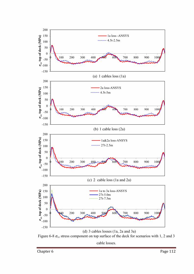
Chapter 6 Page 112

(a) 1 cables loss (1a)

(b) 1 cable loss (2a)

(c) 2 cable loss (1a and 2a)

(d) 3 cables losses (1a, 2a and 3a)

Figure 6-8 σxx stress component on top surface of the deck for scenarios with 1, 2 and 3

cable losses.

-150

-100

-50

0

50

100

150

200

0 100 200 300 400 500 600 700 800 900 1000

σ xx t

op o

f dec

k (M

Pa) 1a loss -ANSYS

4.5t-2.5m

-150

-100

-50

0

50

100

150

200

0 100 200 300 400 500 600 700 800 900 1000

σ xx t

op o

f dec

k (M

Pa) 2a loss-ANSYS

4.5t-5m

-150

-100

-50

0

50

100

150

200

0 100 200 300 400 500 600 700 800 900 1000

σ xx t

op o

f dec

k (M

Pa)

1a&2a loss-ANSYS27t-2.5m

-150

-100

-50

0

50

100

150

200

0 100 200 300 400 500 600 700 800 900 1000

σ xx t

op o

f dec

k (M

Pa) 1a to 3a loss-ANSYS

27t-5.0m27t-7.5m

Chapter 6 Page 113

(a) 1 cables loss (1a)

(b) 1 cable loss (2a)

(c) 2 cable loss (1a and 2a)

(d) 3 cable loss (1a, 2a and 3a)

Figure 6-9 σxx stress component on bottom surface of the deck for scenarios with 1, 2 and 3 cable losses.

-250

-200

-150

-100

-50

0

50

100

0 100 200 300 400 500 600 700 800 900 1000

σ xx b

otto

m o

f dec

k (M

Pa)

1a loss-ANSYS4.5t-2.5m

-250

-200

-150

-100

-50

0

50

100

0 100 200 300 400 500 600 700 800 900 1000

σ xx b

otto

m o

f dec

k (M

Pa)

2a loss-ANSYS4.5t-5m

-250

-200

-150

-100

-50

0

50

100

0 100 200 300 400 500 600 700 800 900 1000

σ xx b

otto

m o

f dec

k (M

Pa)

1a & 2a loss-ANSYS27t-2.55m

-250

-200

-150

-100

-50

0

50

100

0 100 200 300 400 500 600 700 800 900 1000

σ xx b

otto

m o

f dec

k (M

Pa)

1a to 3a loss-ANSYS27t-5.0m27t-7.0m

Chapter 6 Page 114

(a) 1 cables loss (1a)

(b) 1 cable loss (2a)

(c) 2 cable loss (1a and 2a)

(d) 3 cable loss (1a, 2a and 3a)

Figure 6-10 Envelop of the maximum tensile stress over breakage stress in the cables

“a” (z=9.6).

0%

10%

20%

30%

40%

50%

60%

0 5 10 15 20 25 30 35 40 45 50 55 60

Cab

le st

ress

rat

io (%

)

4.5t-2.5m1a loss-ANSYS

0%

10%

20%

30%

40%

50%

60%

0 5 10 15 20 25 30 35 40 45 50 55 60

Cab

le st

ress

rat

io (%

)

4.5t-5.0m2a loss -ANSYS

0%

10%

20%

30%

40%

50%

60%

0 5 10 15 20 25 30 35 40 45 50 55 60

Cab

le st

ress

rat

io (%

)

27t-2.5m1a&2a loss -ANSYS

0%

10%

20%

30%

40%

50%

60%

0 5 10 15 20 25 30 35 40 45 50 55 60

Cab

le st

ress

rat

io (%

)

27t-5m27t-7.5m1a to 3a loss-ANSYS

Chapter 6 Page 115

(a) 1 cables loss (1a)

(b) 1 cable loss (2a)

(c) 2 cable losses (1a and 2a)

(d) 3 cable losses (1a, 2a and 3a)

Figure 6-11 Envelop of the maximum tensile stress over breakage stress in the cables

“b” (z= - 9.6).

0%

10%

20%

30%

40%

50%

60%

0 5 10 15 20 25 30 35 40 45 50 55 60

Cab

le st

ress

rat

io (%

)

4.5t-2.5m1a loss-ANSYS

0%

10%

20%

30%

40%

50%

60%

0 5 10 15 20 25 30 35 40 45 50 55 60

Cab

le st

ress

rat

io (%

)

4.5t-5m2a loss -ANSYS

0%

10%

20%

30%

40%

50%

60%

0 5 10 15 20 25 30 35 40 45 50 55 60

Cab

le st

ress

rat

io (%

)

27t-2.5m1a&2a loss -ANSYS

0%

10%

20%

30%

40%

50%

60%

0 5 10 15 20 25 30 35 40 45 50 55 60

Cab

le st

ress

rat

io (%

)

27t-5m27t-7.5m1a to 3a loss-ANSYS

Chapter 6 Page 116

6.4.3 Comparative study between blast load and simple cable loss according to

ALP (blast near tower and mid-span)

In this section, Scenario: 27t_525m (explosion in the vicinity of cable no. 30a) is

compared with 30a_loss _ANSYS as one of the scenarios in which blast occurs around

the mid-span. Furthermore, Scenario: 27t_225m (explosion in the vicinity of cable 15a)

is compared with 15a_loss _ANSYS as one of the scenarios in which blast occurs

around the tower, respectively.

Deck and Tower

Table 6-4 summarised the maximum deflection in the deck and lateral drift on top of the

tower as well as the maximum σxx stress component on top and bottom surface of the

deck and σeqv on the bottom of tower for all scenarios. Furthermore, deflected

configurations of the deck when maximum vertical displacement has occurred, and

average σxx stress component on the top and bottom surfaces of deck (when maximum

stress has occurred) for blast scenarios with loss of one cable at mid-span and adjacent

to tower are shown in Figures 6-12 (loss of 30a) and Figure 6-13 (loss of 15a),

respectively. Overall, the ALP cable loss analysis has predicted the response of bridge

with accuracy comparable with direct blast analysis. However, the localised large

stresses occurred within the area directly affected by air blast cannot be adequately

captured by the simplistic approach adopted in the alternate load path (ALP) method.

For example, when the detonation centre was near the tower, the direct blast load

analysis predicted σxx stress component on top surface of the deck which is twice as

large the σxx predicted by ALP method (Figure 6-13b). The blast scenarios near mid-

span and tower did not trigger the progressive collapse of the entire bridge according to

ALP method as well as direct blast analysis.

Cable

The cable stresses for scenarios in which cable 30a and cable 15a are lost is presented in

Figure 6-14 and the results are similar to the other scenarios in that no cable exceeded

the breakage stress. Furthermore, cable stresses obtained from blast analysis for short

cables (cable numbers between 10-20 and 40-50) are considerably larger than the results

predicted by ALP cable loss analysis.

Chapter 6 Page 117

(a)

(b)

(c)

Figure 6-12 Maximum of (a) vertical deflection (b) σxx on top of the deck and (c) σxx on

bottom of the deck (loss of cable 30a).

-1

-0.5

0

0.5

0 100 200 300 400 500 600 700 800 900 1000

Ver

tical

dis

plac

emen

t (m

) 30a loss-ANSYS

27t-525m

-150

-100

-50

0

50

100

0 100 200 300 400 500 600 700 800 900 1000

σ xx t

op o

f the

dec

k (M

pa) 30a loss-ANSYS

27t-525m

-150

-100

-50

0

50

0 100 200 300 400 500 600 700 800 900 1000

σ xx b

otto

m o

f the

dec

k (M

Pa)

30a loss-ANSYS

27t-525m

Chapter 6 Page 118

(a)

(b)

(c)

Figure 6-13 Maximum of (a) vertical deflection (b) σxx on top of the deck and (c) σxx on

bottom of the deck (loss of cable 15a).

-1

-0.5

0

0.5

0 100 200 300 400 500 600 700 800 900 1000

Ver

tical

dis

plac

emen

t (m

)

15a loss-ANSYS27t-225m

-200

-150

-100

-50

0

50

100

0 100 200 300 400 500 600 700 800 900 1000

σ xx t

op o

f the

dec

k (M

pa)

15a loss-ANSYS

27t-225m

-150

-100

-50

0

50

0 100 200 300 400 500 600 700 800 900 1000

σ xx b

otto

m o

f the

dec

k (M

Pa)

15a loss-ANSYS

27t-225m

Chapter 6 Page 119

(a) Side-A cable 30a

(b) Side-B cable 30a

(c) Side-A cable 15a

(d) Side-B cable 15a

Figure 6-14 Cable stress ratio (loss of cables 30a/15a).

0%

10%

20%

30%

40%

50%

0 5 10 15 20 25 30 35 40 45 50 55 60

Cab

le st

ress

rat

io (%

)

27t-525m30a loss -ANSYS

0%

10%

20%

30%

40%

50%

0 5 10 15 20 25 30 35 40 45 50 55 60

Cab

le st

ress

rat

io (%

)

27t-525m30a loss -ANSYS

0%

10%

20%

30%

40%

50%

0 5 10 15 20 25 30 35 40 45 50 55 60

Cab

le st

ress

rat

io (%

)

27t-225m15a loss -ANSYS

0%

10%

20%

30%

40%

50%

0 5 10 15 20 25 30 35 40 45 50 55 60

Cab

le st

ress

rat

io (%

)

27t-225m15a loss -ANSYS

Chapter 6 Page 120

6.5 Conclusions

A numerical study of the idealised cable-stayed bridge model subjected to blast loadings

was carried out in this chapter. Also, the results obtained from the blast analysis were

compared with the alternate load path (ALP) cable loss analyses. A comprehensive

parametric study was undertaken and the importance of using a particular model under

several blast loadings as well as sudden loss of cable(s) with non-linear effects was

investigated. With regard to the numerical studies undertaken this chapter, the following

conclusions may be drawn;

- For the bridge under consideration, 1 tonne of TNT equivalent explosive did not

lead to any loss of cables, whereas detonation of 27 tonnes of TNT equivalent

explosive near the end pin support led to loss of three cables.

- Cable(s) were lost due to damage at the anchorage zone rather than the damage

of the cables themselves.

- The dynamic response of the entire cable stayed bridge following loss of the

cables due to blast load can be adequately predicted by alternate load path

(ALP) method regardless of the number of lost cables. The average difference

between the results obtained from the direct blast and ALP cable loss analysis is

around 15% to 25% depending on the location and type of structural

components. However, the localised high stresses and deflections within the

zone directly affected by the air blast cannot be adequately predicted by the ALP

approach. This can be a critical factor when highly localised stresses lead to

failure of a structural component that in turn will trigger the progressive collapse

of the entire bridge.

- The response of the short cables adjacent to towers is sensitive to the choice of

analysis. The stresses in short cables were significantly increased following blast

loading scenarios, however, the stresses in short cables did not considerably

change following different cable loss scenarios.

- For all scenarios, the σxx and σeqv at different components (i.e. deck and tower)

captured by direct blast analysis and ALP cable loss were well below the yield

Chapter 6 Page 121

strength of steel and accordingly no plastic hinge formed within the deck and

tower. Furthermore, loss of up to three cables (either by direct blast analysis or

simple cable removal according to ALP procedure) did not trigger progressive

collapse of the entire bridge.

Chapter 7 Page 122

: Dynamic Response of a Cable-Stayed Chapter 7

Bridge Subjected to Seismic Loading

Summary of chapter Large seismic actions have caused severe damage including progressive collapse of

bridge structures in the past, and are now recognised as one of the most important

extreme loading cases that should be considered in bridge design. In this chapter, a

detailed 3D nonlinear finite element model of a hypothetical cable-stayed bridge is

developed and analysed. The developed FE models can take account of material and

geometrical nonlinearities. A parametric study is undertaken and the effects of seismic

loading scenarios (i.e. different types of earthquake acceleration in terms of frequency

content and amplitude as well as direction) on the local as well as global and potential

progressive collapse response of the bridge are investigated. For the bridge studied in

this chapter, it is shown that the near field earthquakes applied along the bridge length

have the most influence on the deck and cables. Moreover, LS-DYNA FE model and

explicit solver are employed to analysis and capture the possible failure mode of the

cable stayed bridge subjected to severe earthquake action along the bridge deck. It is

shown that the failure mode of the cable stayed bridge under consideration is associated

with development of high plastic strains around the pin support and this is consistent

with the observed failure mode of real cable stayed bridges during past seismic actions.

7.1 Introduction

As discussed in Section 2-5 of Chapter 2, some bridges were damaged or even fully

collapsed by severe past earthquakes. To prevent the catastrophic failure of bridges

subject to earthquake actions, the existing design codes place particular emphasis on

seismic design of bridges and also many studies have resorted to advanced computer-

based simulations to provide a better understanding about the behaviour of bridges

under earthquake attack.

Chapter 7 Page 123

With regard to high cost of undertaking field or lab test, one of the options for structural

assessment of large scale bridges is to use advanced computer simulations (e.g. finite

element models) that can properly capture the local and global response of the structure

including material and geometrical nonlinearities.

In this chapter, using ANSYS package (ANSYS® 2009) as well as LS-DYNA (LSTC

2007), 3D FE models of the bridge are developed and analysed under gravity loads,

traffic load and different seismic ground acceleration scenarios. Using the developed FE

models, a comprehensive parametric study is carried out and structural response of the

bridge under different peak ground accelerations and direction of earthquake attack is

studied. Furthermore, the results obtained from a fully nonlinear 3D FE model are

employed to identify the critical earthquake acceleration and direction range for each

one of the structural components (i.e. deck, towers, cables and base shear).

With regard to lack of experimental data on cable-stayed bridge models, the

preparations for future experimental works on a 1/60 scale cable-stayed bridge are

presented in the final section of this chapter. The experimental work of this study

follows previous shake table test of a 1/120 scale pre-stressed concrete cable stayed

bridge model undertaken by Shoji et. al (2008).

7.2 Adopted assumptions

The adopted assumptions including bridge geometry and configuration, material

properties including yield and ultimate strength of steel and ultimate strength of cable,

3D finite element (FE) models developed in ANSYS and LS-DYNA, analysis methods

and design loads in this chapter are the same as those in Chapter 6, Sections 6.2.

To start the seismic analysis of the cable stayed bridge, an eigenvalue analysis was

carried out and the frequency, period and mode shape of the first fifteen natural modes

of vibration were extracted from the results of this eigenvalue analysis. The first six

mode shapes of the bridge obtained from eigenvalue analysis of the 3D-implicit FE

model developed in ANSYS software is shown in Figure 7-1. Furthermore, the natural

frequency and period of the first fifteen modes of vibration are given in Table 7-1.

Chapter 7 Page 124

7.3 Seismic analysis scenarios

7.3.1 Seismic analysis method

Transient (time-history) analysis of the bridge was carried out using a direct time

integration to determine the dynamic responses of the bridge model subjected to seismic

loads. For the dynamic time marching, two different integration methods were used; i.e.

Newmark constant acceleration method was used in conjunction with ANSYS implicit

solver (ANSYS, 2009) and a central difference scheme was used in conjunction with

LS-DYNA explicit solver (LSTC, 2007; Paz 2004). In both implicit and explicit

models, a consistent mass matrix with proportional damping was adopted. In ANSYS

software, “ACEL” command, which specifies the linear acceleration in the global

Cartesian, x, y, and z coordinates, was used for applying the seismic load. Using this

command, the same seismic acceleration was applied on all elements at the same time.

In LS-DYNA program, “LOAD_BODY_option” code with a feature similar to “ACEL”

commands of ANSYS was employed for applying the seismic action (ground

acceleration); The “LOAD_BODY_option” can be used to activate the mass of the

structure in conjunction with prescribed base accelerations in a Cartesian coordinate

system.

Table 7-1 The natural frequency and period of the first fifteen modes of vibration.

Mode No. Frequency (Hz) Vibration Period (sec) 1 0.055 18.2 2 0.172 5.81 3 0.237 4.22 4 0.285 3.51 5 0.342 2.92 6 0.458 2.18 7 0.505 1.98 8 0.532 1.88 9 0.582 1.72 10 0.616 1.62 11 0.651 1.54 12 0.716 1.40 13 0.721 1.39 14 0.722 1.39 15 0.731 1.37

Chapter 7 Page 125

Figure 7-1 The natural period and mode shapes for the first 6 natural modes of

vibration.

(a) 1st mode (T= 18.2 sec) (b) 2nd mode (T= 5.81sec)

(c) 3rd mode (T=4.22 sec) (d) 4th mode (T= 3.51sec)

(f) 5th mode (T= 2.92sec) (e) 6th mode (T= 2.18sec)

Chapter 7 Page 126

7.3.2 Scenario considered for Earthquake load analysis

For seismic analysis, the distributed component of the traffic load as well as the dead

load is applied along the entire bridge deck. The adopted load factors for dead, live and

earthquake actions (loads) are as specified by AASHTO LRFD bridge design code and

also reported in NCHRP (2003),

1.25 0.25 1.0DC LL EQ (1)

where, DC is the permanent action (dead load) including self-weight of structural

components and non-structural attachments, LL is the full vehicular live load placed in

actual stripped lanes and EQ is the earthquake load. In this study, the wearing surface is

assumed to be a 200 mm thick layer of asphalt concrete ( =24.5 kN/m3) which is

considered as part of permanent action (dead load).

According to AS5100.2 (2004), for the loading scenarios in which more than one lane is

subjected to traffic loads, the traffic loads should be multiplied by an accompanying

lane factor (1.0 for first lane, 0.8 for second lane and 0.4 for third and subsequent

lanes). In this chapter, the traffic loading pattern and accompanying lane factor are as

specified in Figure 5-2b in Chapter 5.

7.3.3 Earthquake acceleration data

Both near-field and far-field earthquake records were used in this analysis; namely

Kobe (Japan, 1995) and El-Centro (USA, 1940). Time-histories of ground accelerations,

as well as acceleration response spectra for both earthquakes are shown in Figure 7-2a

and 7-2b, respectively. In Figure 7-2a, Kobe record shows jerky high peak accelerations

of over 8 m/s2. This pulse-like ground motions normally create significant damage to

the structures, including bridge structures (Liel, 2012, Moustafa and Takewaki, 2010,

Jia and Ou, 2008). On the other hand, the frequency content of the El-Centro ground

acceleration spreads over a wide range with less fluctuation. With regard to acceleration

response spectra given in Figure 7-2b, it is concluded that the dominant frequency range

possessing much of the seismic energy for Kobe earthquake is in the range between 0.5

to 3.5 Hz, whereas for El-Centro earthquake the range of dominant frequency content is

between 0.5 to 7.5 Hz.

Chapter 7 Page 127

(a)

(b)

Figure 7-2 (a) ground acceleration time history (b) acceleration response spectrum.

7.3.4 Scenarios considered

A total of nine different seismic loading scenarios were considered in this study as

summarised in Table 7-2. In the first five scenarios, i.e. Scenario-K1 to scenario-K5

Kobe earthquake ground acceleration is applied on the bridge and in the last four

scenarios, i.e. scenario E1 to E4, the El-Centro earthquake is considered. In terms of

magnitude and direction of ground acceleration, scenarios K1 and K5 are the same and

the difference between these two scenarios is only related to the type of FE solver that

will be explained later (see Table 7-2).The ground accelerations are applied horizontally

to the bridge in different directions, i.e. along the deck (x-direction), perpendicular to

the bridge deck (z-direction), 30 and 60 degrees between the x and z axes.

-10

-8

-6

-4

-2

0

2

4

6

0 10 20 30 40 50 60G

roun

d ac

cele

ratio

n (m

/s2 )

Time (seconds)

KobeElcentro

0

100

200

300

400

0 1 2 3 4 5 6 7 8

Acc

elet

ratio

n re

spon

se sp

ectr

um (g

/100

0)

Frequency (Hz)

KobeElcentro

Kobe frequency content

Elcentro frequency content

Chapter 7 Page 128

Table 7-2 Scenarios considered for applying seismic action.

Scenario No. Name of earthquake EQ Direction FE method

Scenario-K1

Kobe

x Implicit Scenario-K2 z Implicit Scenario-K3 30° xz Implicit Scenario-K4 60° xz Implicit Scenario-K5 x Explicit Scenario-E1

El-Centro

x Implicit Scenario-E2 z Implicit Scenario-E3 30° xz Implicit Scenario-E4 60° xz Implicit

7.4 Results and discussion

In this section, the analysis results produced by ANSYSS implicit model for Scenarios

K2 to K4 and E1 to E4 are presented and discussed. The ANSNS implicit dynamic

model stopped after 9.8 seconds into the Kobe earthquake applied along the bridge deck

(Scenario-K1). A closer look to the ANSYS FE results showed large plastic strains in

conjunction with large displacements occurring around the pin support that led to ill

conditioning and subsequently lack of convergence in ANSYS implicit model.

Accordingly, scenario K1 and the cause of convergence problem in ANSYS implicit

model are discussed in details and the results of scenario K5 obtained from LS-DYNA

explicit model are presented.

7.4.1 Results of implicit analysis (ANSYS model)

Deck and tower

Table 7-3 summarises the maximum deflections, maximum nodal σxx stresses on the

deck and drift on top and σeqv stress at the bottom of the right tower occurring during

each earthquake as well as the corresponding values for the healthy bridge (Scenario-

SH) in the absence of seismic loads and only under gravity loads. Also, the deflected

configurations (elastic curve) of the deck at the instant of maximum vertical

displacement for all seismic load scenarios are shown in Figure 7-3. It is observed that

scenario K3 can create significant hogging deflection (1.52 m uplift) in the back span at

x= 150 m. Furthermore, it is seen that the major longitudinal flexural stresses along the

deck (see Table 7-3) exceed the yield strength of steel (450MPa) in scenario-K series.

Chapter 7 Page 129

Accordingly, xx stresses on top and bottom surface of the deck in scenario-K3 (most

critical) are plotted in Figure 7-4. The zone in which the stress xx exceeding the yield

stress is quite localised and only limited to close proximity of the pin-support.

Table 7-3 Summary of the maximum vertical deflections, drift on top of right tower and

xx stresses within the deck obtained from implicit 3D ANSYS FE models.

Deck Tower

δy+ (m) δy- (m) σxx (MPa) δtopx (m) δtopz (m) σbot eqv (MPa)

Scenario-SH# 0.22 -0.37 317.7 (C) -0.33 0.00 91.6 Scenario-K1 Scenario-K2 0.33 -0.49 508.9 (T) -0.37 0.69 198.0 Scenario-K3 1.55 -1.07 558.4 (T) -1.09 0.34 281.0 Scenario-K4 0.92 -0.73 535.3 (T) -0.80 0.60 263.3 Scenario-E1 0.47 -0.50 319.3 (C) -0.49 0.00 135.6 Scenario-E2 0.27 -0.42 436.4 (T) -0.34 -0.14 115.0 Scenario-E3 0.43 -0.49 425.1 (T) -0.47 -0.06 138.8 Scenario-E4 0.35 -0.45 467.5 (T) -0.41 -0.10 130.4

# Healthy bridge subject to gravity (dead load including wearing surface + traffic) load.

(a)

(b)

Figure 7-3 Vertical deflection along the deck (a) Scenario K2-K4 (b) Scenario E1-E4.

-0.8

-0.4

0

0.4

0.8

1.2

1.6

0 100 200 300 400 500 600 700 800 900 1000

Ver

tical

def

lect

ion

(m)

Scenario-K2Scenario-K3Scenario-K4

-0.6

-0.4

-0.2

0

0.2

0.4

0 100 200 300 400 500 600 700 800 900 1000

Ver

tical

def

lect

ion

(m) Scenario E1

Scenario E2Scenario E3Scenario E4

Chapter 7 Page 130

(a)

(b)

Figure 7-4 σxx stress component on the (a) top and (b) bottom surface of the deck for

scenario-K3 compared with healthy structure

Cables

Envelope of maximum tensile stresses in the cables expressed as a percentage of cable

ultimate strength for scenarios K2 to K4 and E1 to E4, as well as the healthy bridge

under gravity load (i.e. scenario-SH) are shown in Figure 7-5. It is seen that the

maximum tensile stresses in some of the cables during scenario K3 and K4 reached the

80% of cable breakage stress. The critical cables under the Kobe earthquake loading

scenarios are amongst the short cables in the vicinity of towers (see Figure 7-5a).

-100

-50

0

50

100

150

0 100 200 300 400 500 600 700 800 900 1000

σ xx t

op o

f dec

k (M

Pa) Scenario-K3

Scenario-SH

-200

-100

0

100

200

300

400

500

600

0 100 200 300 400 500 600 700 800 900 1000σ xx b

otto

m o

f dec

k (M

Pa)

Scenario-K3Scenario-SH

Yield strength

Localised plastic zone

Chapter 7 Page 131

(a)

(b) Figure 7-5 Envelop of the maximum tensile stress over ultimate strength in the cables

(a) Scenarios K2-K4 and (b) Scenarios E1-E4.

7.4.2 Progressive collapse analysis – Scenario K1

Deck and tower

The deflected configuration (elastic curve) of the deck at 9.7 sec into seismic loading

scenario-K1 (one step just before the occurrence of convergence problem in ANSYS

implicit model) and the xx stress on top and bottom surface of the deck for Scenario-

K1 are shown in Figure 7-6.

0%

20%

40%

60%

80%

100%

120%

0 10 20 30 40 50 60

Stre

ss r

atio

(%)

Cable No.

Scenario SHScenario K2Scenario K3Scenario K4

20%

30%

40%

50%

60%

0 10 20 30 40 50 60

Stre

ss r

atio

(%)

Cable No.

Scenario SHScenario E1Scenario E2Scenario E3Scenario E4

Chapter 7 Page 132

(a)

(b)

(c)

Figure 7-6 (a) has occurred along with xx stress components on the (b) top and (c)

bottom surface of the deck for scenario-SH (only gravity loads) and scenario-K1.

-0.4-0.3-0.2-0.1

00.10.20.30.40.5

0 100 200 300 400 500 600 700 800 900 1000

Ver

tical

def

lect

ion

(m)

Scenario-K1Scenario-SH

-300

-200

-100

0

100

0 100 200 300 400 500 600 700 800 900 1000

σ xx o

n to

p of

dec

k (M

Pa)

Scenario-K1Scenario-SH

-500

-400

-300

-200

-100

0

100

0 100 200 300 400 500 600 700 800 900 1000

σ xx o

n bo

ttom

of d

eck

(MPa

)

Scenario-K1Scenario-SH

Yield strength of steel

Localised plastic zone

Chapter 7 Page 133

With regard to Figure 7-6a, it is observable that the deflections of deck occurred under

seismic loading scenario-K1 are not that large compared with the deflections of deck

only under gravity load (i.e. scenario-SH). The xx stresses along the top surface of the

deck (see Figure 7-6b) are not critical (well below the yield strength), whereas the xx stresses on the bottom surface of the deck (Figure 7-6c) at the sections x= 7.5-17.5 m

away from the pin-support exceeded the yield strength (450 MPa) of steel and led to

formation of a plastic hinge at this section. The large plastic strains and rotations

occurred at this plastic hinge must be the reason that ANSYS implicit model

encountered convergence problem and stopped at 9.8 seconds into the seismic loading

scenario-K1. To capture the possible collapse and failure mode of the structure, the

bridge was modelled and analysed using LS-DYNA software and its explicit solver.

The scenario-K5 in which the Kobe earthquake is applied along the bridge deck (x-

direction) is considered in this section. As explained in Section 6.2.2 in Chapter 6, the

elements in LS_DYNA will be deactivated when the plastic strain within the element

reaches the plastic strain corresponding to failure of steel that is taken as 0.06 inhere.

The results of xx stress along the bottom of the deck at 9.7 seconds into the

earthquake loading obtained from Scenarios K1 and K5 are compared and shown in

Figure 7-7a that demonstrates a good correlation between the two FE models (i.e. ANSYS

implicit and LS_DYNA explicit). Moreover, Figure 7-7b shows the time history of xx stress at section x= 7.5 m away from the pin support, where the highest nodal xx

stresses were observed. It is seen that the stress at this location exceeds the yield

strength a couple of times, however, after 12 seconds into seismic loading scenario, the

xx stress drops and fluctuates around 0 MPa.

The contour of stress and plastic strain on the bottom of the deck around pin-support

(x= 0 to x= 40 m) at selected instants are shown in Figure 7-8. The stress and strain at

9.7 seconds, when the convergence criteria are still met in the ANSYS implicit FE

model are shown in Figure 7-8a. The xx stresses above yield strength of steel (i.e.

450MPa) are observable in Figure 7-8a, however, the plastic strains are still very small

(close to zero) at this stage. At 11.65 seconds (Figure 7-8b), the plastic strains start to

develop. Following that, at 11.82 seconds, two elements are eliminated since these

Chapter 7 Page 134

elements have reached the plastic strain corresponding to failure (taken as 0.06). At

11.95 seconds, four more elements were eliminated. After this stage, no element

reached the failure point, however, the damaged zone was squeezed at around 30

seconds as shown in Figure 7-8e, that can be indicative of local buckling and large

displacements/rotations (see Figure 7-8f). The failure mode predicted by the LS_DYNA

explicit model (Figure 7-9a) is associated with significant up-lift around the pin support

and also it correlates reasonably well with those observed in the Higashi-Kobe Bridge

(Figure 7-9b) in the aftermath of Kobe earthquake.

(a)

(b)

Figure 7-7 (a) σxx on bottom of the deck at 9.7 seconds and (b) time history of σxx at

x= 7.5 m (stress exceeded the yield strength at 9.7 sec).

-500

-400

-300

-200

-100

00 200 400 600 800 1000

σ xx o

n bo

ttom

of d

eck

(MPa

)

LS-DYNAANSYS

-500-400-300-200-100

0100200300400500

0 5 10 15 20 25 30

Tim

e hi

stor

y of

σxx

@ x

=7.5

m

Time (seconds)

Yield strength of steel

Yield strength of steel

Yield strength of steel

Chapter 7 Page 135

(a) 9.7 seconds

(b) 11.65 seconds

(c) 11.82 seconds

(d) 11.95 seconds

(e) 30 seconds

(f) 60 seconds

Figure 7-8 σxx and plastic strain around pin-support using ANSYS and LS DYNA

Chapter 7 Page 136

(a)

(b)

Figure 7-9 (a) Bridge configuration at 60 seconds (after earthquake) and (b) uplift of the

deck around the pin-support, Higashi-Kobe Bridge after 1995 Kobe Earthquake.

Figure 7-10 Time history of σeqv at the bottom of towers.

0

100

200

300

400

500

0 10 20 30 40 50 60

σ eqv

bot

tom

of t

ower

Time (second)

Left towerRight tower

Yield strength of steel

Side view

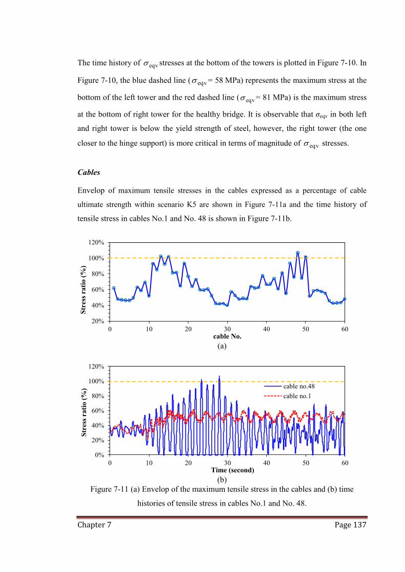
Chapter 7 Page 137

The time history of eqv stresses at the bottom of the towers is plotted in Figure 7-10. In

Figure 7-10, the blue dashed line ( eqv = 58 MPa) represents the maximum stress at the

bottom of the left tower and the red dashed line ( eqv = 81 MPa) is the maximum stress

at the bottom of right tower for the healthy bridge. It is observable that σeqv in both left

and right tower is below the yield strength of steel, however, the right tower (the one

closer to the hinge support) is more critical in terms of magnitude of eqv stresses.

Cables

Envelop of maximum tensile stresses in the cables expressed as a percentage of cable

ultimate strength within scenario K5 are shown in Figure 7-11a and the time history of

tensile stress in cables No.1 and No. 48 is shown in Figure 7-11b.

(a)

(b)

Figure 7-11 (a) Envelop of the maximum tensile stress in the cables and (b) time

histories of tensile stress in cables No.1 and No. 48.

20%

40%

60%

80%

100%

120%

0 10 20 30 40 50 60

Stre

ss r

atio

(%)

cable No.

0%

20%

40%

60%

80%

100%

120%

0 10 20 30 40 50 60

Str

ess r

atio

(%)

Time (second)

cable no.48cable no.1

Chapter 7 Page 138

It is observable that in the earthquake loading scenario K5, the shorter cables (i.e. cables

adjacent to the towers) are more critical than longer cables. The maximum tensile stress in

the short cables (such as No. 13, 15, 48 and 50) has reached the breakage stress of the

cables. However, the bridge model did not show any zipper type of collapse during this

earthquake (i.e. scenario K5), because the most critical cables which their rupture can

potentially trigger the progressive collapse of the cable stayed bridges are the ones

connected to the pin support or mid-span (i.e. the longest cables such No.1 or 30). Also, the

stress in the critical cables (e.g. No. 48) exceeds the breakage stress at only one instant.

7.5 Effect of traffic load distribution on the seismic response

In this section, the effect of traffic load distribution along the bridge deck on the

potential progressive collapse response of the cable stayed bridge subject to seismic

actions is investigated. The three different loading pattern (traffic load distribution)

considered in this section is shown in Figure 7-12.

In conjunction with these loading patterns (see Figure 7-12), scenario-K5 (Kobe

earthquake along the bridge deck) was considered to produce the maximum vertical

deflection and maximum stresses in the structural components (i.e. deck and cables).

(a) Traffic load is distributed along the entire bridge (Entire Bridge)

(b) Traffic load is only acting on the middle span (Middle)

(c) Traffic load is only acting on the side spans (Side)

Figure 7-12 Traffic load distribution.

Chapter 7 Page 139

The average xx stress on the bottom of the deck (along the deck) around 10 seconds

into the earthquake (when the maximum stress occurred during the seismic event) for

scenario-K5 is shown in Figure 7-13. Applying the traffic load on the entire bridge or

on the side span led to the most critical scenarios in terms of maximum xx stresses

induced in the deck. When the traffic load was applied on the entire bridge, the

compressive xx stress reached the yield strength of steel at sections around the pin

support, whereas applying the traffic load only on the side spans led to maximum

tensile xx stresses.

The envelop of vertical deflection and average xx stress on the bottom surface of the

deck at 60 seconds into the K5 earthquake scenario are shown in Figures 7-14a and b,

respectively. The loading pattern in which the traffic load is applied only on the side

span shows up-lift at the middle-span and sagging effect in the vicinity of the pin

support whereas applying the traffic load on the entire span or only on the middle-span

leads to sagging deflections over middle span and hogging deflections over end (side)

spans. The maximum deflection during earthquake scenario K5 occurred when the

traffic load was applied only on the middle-span. After the Kobe earthquake (60

seconds into the K5 earthquake scenario), the residual xx stresses at the bottom of the

deck were within the elastic range (see figure 7-14b).

Figure 7-13 σxx on bottom of the deck around 10 seconds into the K5 earthquake

scenario (first element reached the plastic strain).

-500-400-300-200-100

0100200300400500

0 100 200 300 400 500 600 700 800 900 1000

xx b

otto

m o

f dec

k (M

Pa)

Middle-spanSideEntire bridge

Yield strength of steel

Yield strength of steel

Chapter 7 Page 140

(a)

(b)

Figure 7-14 Envelop of (a) vertical displacement and (b) σxx on the bottom surface of

the deck at 60 seconds into the K5 earthquake scenario.

Envelop of maximum tensile stresses in the cables expressed as a percentage of cable

ultimate strength within earthquake scenario K5 for three different traffic load patterns are

shown in Figure 7-15. It is observed that the maximum tensile stresses occur in the short

cables (e.g. No. 13, 15, 48 and 50) when the traffic loads are applied on the entire bridge

and side spans. In the short cables No. 13, 15, 48 and 50, the tensile stresses have reached

the breakage stress of the cables. When the traffic load was applied on the middle-span,

cable no.1 reached 90% of the breakage stress. Such a scenario is critical, because cable

no.1 is one of the cables that its loss can potentially trigger the zipper type of collapse.

-4

-2

0

2

4

6

0 100 200 300 400 500 600 700 800 900 1000

Ver

tical

dis

plac

emen

t (m

) Middle-spanSideEntire bridge

-500-400-300-200-100

0100200300400500

0 100 200 300 400 500 600 700 800 900 1000

xx b

otto

m o

f dec

k (M

Pa)

Middle-spanSideEntire bridge

Yield strength of steel

Yield strength of steel

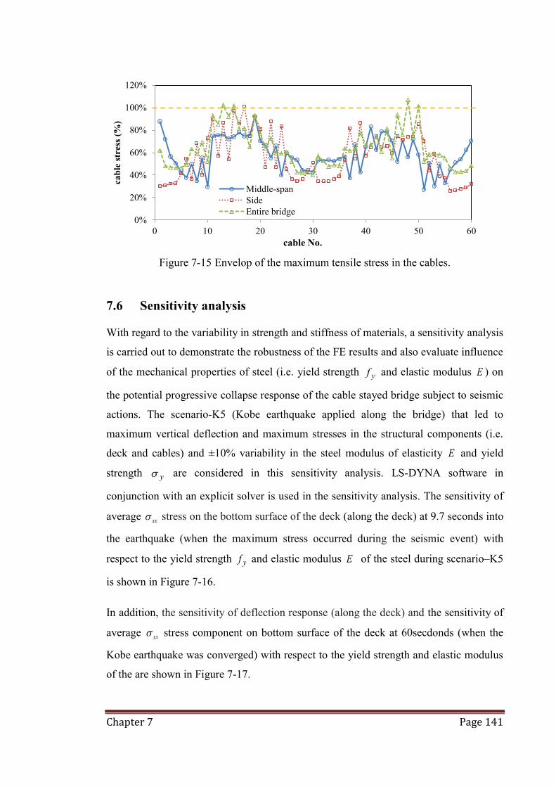
Chapter 7 Page 141

Figure 7-15 Envelop of the maximum tensile stress in the cables.

7.6 Sensitivity analysis

With regard to the variability in strength and stiffness of materials, a sensitivity analysis

is carried out to demonstrate the robustness of the FE results and also evaluate influence

of the mechanical properties of steel (i.e. yield strength yf and elastic modulus E ) on

the potential progressive collapse response of the cable stayed bridge subject to seismic

actions. The scenario-K5 (Kobe earthquake applied along the bridge) that led to

maximum vertical deflection and maximum stresses in the structural components (i.e.

deck and cables) and ±10% variability in the steel modulus of elasticity E and yield

strength y are considered in this sensitivity analysis. LS-DYNA software in

conjunction with an explicit solver is used in the sensitivity analysis. The sensitivity of

average xx stress on the bottom surface of the deck (along the deck) at 9.7 seconds into

the earthquake (when the maximum stress occurred during the seismic event) with

respect to the yield strength yf and elastic modulus E of the steel during scenario–K5

is shown in Figure 7-16.

In addition, the sensitivity of deflection response (along the deck) and the sensitivity of

average xx stress component on bottom surface of the deck at 60secdonds (when the

Kobe earthquake was converged) with respect to the yield strength and elastic modulus

of the are shown in Figure 7-17.

0%

20%

40%

60%

80%

100%

120%

0 10 20 30 40 50 60

cabl

e st

ress

(%)

cable No.

Middle-spanSideEntire bridge

Chapter 7 Page 142

Figure 7-16 σxx on the bottom of deck at 9.7 seconds into the K5 earthquake scenario.

(a)

(b)

Figure 7-17 (a) Deflected configuration of the deck and (b) σxx on the bottom surface of

the deck at 60 seconds into the K5 earthquake scenario.

-500

-400

-300

-200

-100

0

1000 100 200 300 400 500 600 700 800 900 1000

σ xx

bott

om o

f dec

k (M

Pa)

fy=400 MPa E=180 GPafy=400 MPa E=200 GPafy=400 MPa E=220 GPafy=450 MPa E=200 Gpa -cable breakge=1700MPafy=400 MPa E=220 GPa

-8.0

-6.0

-4.0

-2.0

0.0

2.0

4.0

6.0

8.00 100 200 300 400 500 600 700 800 900 1000

Ver

tical

dis

plac

emen

t (m

)

fy=400 MPa E=180 GPafy=400 MPa E=200 GPafy=400 MPa E=220 GPafy=450 MPa E=200 GPa -cable breakage=1700MPafy=450 MPa E=200 Gpa

-500-400-300-200-100

0100200300400500

0 100 200 300 400 500 600 700 800 900 1000

σ xx

bot

tom

of d

eck

(MPa

)

fy=400 MPa E=180 GPafy=400 MPa E=200 GPafy=400 MPa E=220 GPafy=450 MPa E=200 GPa -cable breakage=1700MPafy=450 MPa E=200 Gpa

Yield strength of steel = 400MPa

Yield strength of steel = 450MPa

Max. Hogging

Max. Sagging

y

y y y y

y

y y y y

y

y y y y

Chapter 7 Page 143

It is observable that the xx stress on the bottom of the deck can exceed the yield

strength of steel at 9.7 seconds into the K5 earthquake scenario. Accordingly, the deck

cross sections in the vicinity of the pin support are identified as the most critical

sections within along the deck earthquake loading scenarios. Moreover, the vertical

deflection, especially maximum hogging around the pin support is quite critical during

earthquake loading scenarios.

Moreover, envelop of maximum tensile stresses in the cables expressed as a percentage of

cable ultimate strength within scenario K5 is shown in Figure 7-18. It is observed that the

maximum tensile stress in the short cables (such as No. 13, 15, 48 and 50) has reached the

breakage stress of the cables. In some of the models, the tensile stress in the cables

exceeded the cable breakage stress; however, no cable loss occurred. Furthermore, the

bridge model did not show any zipper type of progressive collapse during this earthquake

loading scenarios.

Finally, Table 7-4 summarises the timing when the first element reached to the plastic strain

p=0.06) and total number of lost elements due to plastic strain failure. With regard to the

results shown in Table 7-4, it is seen that the deflected configuration of the deck

(locations of maximum sagging and hogging deflection) is sensitive, however, the

variation of stress along the deck (locations of maximum ) are not sensitive to the yield

strength and elastic modulus of steel. This is clearly demonstrative of the robustness as

well as adequacy of the results obtained from the FE models.

Figure 7-18 Envelop of the maximum tensile stress in the cables

0%

20%

40%

60%

80%

100%

120%

0 10 20 30 40 50 60

cabl

e st

ress

(%)

sy=400 MPa E=180 GPasy=400 MPa E=200 GPasy=400 MPa E=220 GPasy=450 MPa E=200 GPa -cable breakage=1700MPasy=450 MPa E=200 Gpa

y

y y y y

Chapter 7 Page 144

Table 7-4 Summary of sensitivity analysis results.

Scenario name

yield stress (MPa)

young's modules (GPa)

Instant of time when plastic

strain occurred

Number of lost

elements

y=400 MPa E=180 GPa 400 180 33.1 sec 218

y=400 MPa E=200 GPa 400 200 31.4 sec 206

y=400 MPa E=220 GPa 400 220 30.4 sec 225

y=450 MPa E=200 GPa 450 200 31.4 sec 216 y=450 MPa E=200 Gpa

cable strength= 1700MPa 450 200 38.8 sec 196

7.7 Preparing for experimental work

To verify the numerical analysis, an experimental work was planned and initiated by the

candidate for the next phase of this research but was deemed beyond the scope of the

current program.

7.7.1 Numerical model

At first, a steel cable stayed bridge model, inspired by Okuwaka Bridge in Japan

(JSCE, 2010), was designed according to AS5100 (AS5100.2, 2004). The dimensions of

the bridge and geometry of sections as well as the configuration of cables for the bridge

considered in this chapter are shown in Figure 7-19.

The full scale bridge is symmetric and has a total span length of 120 m supported by a

single 55 m tall tower and 6 pairs of cables spaced (20 m apart) along the deck.

Furthermore, all cables are regularly spaced (5 m apart) over the tower. The bridge deck

is 25 m wide (4 traffic lanes according to AS5100.2 (2004) and 1.5 m deep and is made

of a multi-cell steel box girder as depicted in Figure 7-19b. This bridge deck is

restrained by pin support at the far left end and by roller support at the far right end

(Figure 7-19a), and there is no direct connection between the deck and the pylons. The

fully fixed cross section of tower leg is shown in Figure 7-19c.

The modulus of elasticity, E , and the yield stress of steel, y , as well as the geometrical

properties of the deck, including second moment of area, I , and cross sectional area ,

,A , are given in Table 7-5.

Chapter 7 Page 145

(a) Bridge configuration

(b) Deck

(c) Tower

Figure 7-19 Configuration for numerical model

x

y

z

y

x

z z

y

Chapter 7 Page 146

Table 7-5 Deck properties.

Numerical

model

Geometric scaling factor (λ=1/50)

numerical model x

scaling factor

Exp. values difference

Material Steel PVC Density (kg/m3) 7850 λ3 1300

Modulus of Elasticity

(MPa) 2.00E+05 λ 4.00E+03 3.80E+03 -5%

A (m2) 1.40E+00 λ2 5.58E-04 5.72E-04 3%

I (m4) 6.94E-01 λ4 1.11E-07 1.14E-07 3%

EI (Nm2) 1.39E+11 λ5 4.44E+02 4.35E+02 -2%

EA (m2) 2.79E+11 λ3 2.23E+06 2.17E+06 -3%

Weight (N) 1.29E+07 λ3 1.03E+02 1.75E+01 -83%

Mass (kg) 1.31E+06 λ3 1.05E+01 1.78E+00 -83%

7.7.2 Design for experimental model

In this study, the geometric scaling-factor is set at 1/50. A prototype model should be

designed and developed with the properties listed in Table 7-4. According to this list,

PVC (Poly Vinyl Chloride) was selected with the modulus of elasticity of 3.8 MPa

(about 1/50 of steel material). A simple drawing for the bridge configuration, including

cross sectional areas of deck and tower for this bridge model, is shown in Figure 7-20.

By comparison, the cross-section of the numerical cross section is somewhat different

because of satisfying the factors EA and EI (see Table 7-5). The error ranges are within

10%.

PVC sheets for deck and tower were cut into several pieces and glued together. In the

numerical model, the deck is supported by pin- and roller-support at each end. For the

experimental model, pin- and roller-support are created by PVC roller installed into a

bearing system as shown in Figure 7-21.

For cables, springs (see Figure 7-22) are installed which have 1/50 of the cable stiffness

compared with the numerical model. Also, cables are connected by 4 forks and springs

see in Figure 7-22.

Chapter 7 Page 147

(a) Bridge configuration

(b) Deck

(c) Tower

Figure 7-20 Experimental bridge model (dimensions in mm)

z

y

z

y

x

z

x

y

Chapter 7 Page 148

(a) Pin support system (b) Roller support system

Figure 7-21 End support system for experimental prototype

Figure 7-22 Devised mechanism for post-tensioning the cables.

7.7.3 Pre-test

The prototype bridge (see Figure 7-23) was attached to the shake table and the first pre-

test was done. Two LVDTs were installed on the top of the tower and left side of the

deck, and 11 accelerometers were placed around the deck and tower side. As can be

seen clearly, cables look too heavy compared with the other segments. In reality, weight

of the cables should be negligible. Thus, in the initial prototype testing, cable vibrations

constituted the first natural frequencies which is not supposed to be the case according

to the numerical analyses.

Forks Spring Rigid wire (3mm)

Chapter 7 Page 149

7.7.4 Re-modelling

According to this pre-testing, the cable material should be changed in order to satisfy

the model properties. Once this is done, the experimental test can continue. The plan is

to use 4 different scaled earthquake ground accelerations.

(a) Bridge model on the shake table

(b) LVDT

(c) Accelerometers

Figure 7-23 (a) Prototype on the shake table, (b) LVDT and (c) accelerometer

Chapter 7 Page 150

7.8 Concluding remarks

A numerical study of an idealised cable-stayed bridge model subjected to four seismic

ground excitations was carried out in this chapter. A comprehensive parametric study

was undertaken and the importance of using a representative model under several

seismic loadings with non-linear effects was investigated. With regards to the

parametric studies in this chapter, the following conclusions can be drawn;

- The earthquake load applied longitudinally (along x-direction) and at 30-degree

to this direction created the highest deformation and stresses in the deck. This

was particularly the case for Kobe earthquake loading scenarios.

- Implicit analysis carried out using ANSYS software encountered some

convergence problem owing to high stress concentration and large deformations.

The numerical convergence issue was particularly severe when Kobe earthquake

was applied along the bridge deck.

- The stress in the towers remained below the yield strength of steel in all of the

considered seismic loading scenarios. In the deck, the sections in the vicinity of

the pin support were identified as the most critical sections in terms of stresses

induced in the deck during earthquake loading scenarios.

- The short stays adjacent to the towers were found to be the most critical ones in

terms of maximum tensile stress induced in the cables during seismic actions.

The stress in these short cables exceeded the breakage stress of cables during

Kobe earthquake when applied longitudinally or at 30-degrees; however, no

cable loss occurred during these earthquake loading scenarios.

- Significant vertical displacement of the deck (hogging) occurred around the pin

support by longitudinal earthquake excitation. These large hogging deflections

were associated with permanent damage in the deck.

- The bridge model studied in this model was not subjected to zipper-type

collapse although the formation of plastic hinges within the deck did occur.

Chapter 8 Page 151

: Conclusions Chapter 8

8.1 Summary of each chapter

Dynamic responses of a hypothetical cable-stayed bridge under several severe

conditions (such as sudden loss of cable, blast loading and seismic loading) were

studied in this thesis. Finite element (FE) models of a cable-stayed bridge designed

according to Australian standards was developed and analysed statically and

dynamically as part of this research. Two commercial FE programs, namely, ANSYS

and LS-DYNA, were used.

Chapter 3:

One of the most critical situations for a cable stayed bridge is the sudden loss of cable(s)

which can be the cause of potential progressive collapse. As discussed in Chapter 2,

some standards, such as PTI, recommend considering any single loss of cable in the

design phase by static analysis using a Dynamic Amplification Factor (DAF) set at 2.

However, due to bridge characteristics (a complex multi degree of freedom system),

DAF=2 has been questioned and investigated in some research works and concluded

that a simplified approach (with DAFs set at 2) could be seemingly quite unsafe since

some of the DAFs could exceed this limit significantly. It is, therefore, recommended to

conduct a dynamic analysis for evaluating the response of the bridge subjected to a

sudden loss of cable. In this thesis, the DAFs associated with different locations, load

durations and number of lost cables were investigated along with the effect of damping

ratio. Moreover, the relationship between DAFs and the potential of progressive

collapse were determined. The studies on DAFs were done by using a liner 2D model.

Therefore, the potential progressive collapse was instead presented by Demand-

Capacity Ratio (DCR). Based on this new relationship, the most critical cable(s) were

determined. The key conclusions were as following:

- The loss of the longest back stays are the most critical ones (the highest DCR values

were observed for all structural components).

- The DAF for the bending moment and axial force at different sections along the

deck, towers and cables can take values much higher than two (typically adopted by

Chapter 8 Page 152

different guidelines), however, the DCR value is usually less than 100% in most

such cases. In other words, material nonlinearity has minor effect on the global

progressive collapse response of the bridge due to cable loss, and it is not un-

conservative to allow a DAF of greater than two as long as DCR remains below one.

- The DAF values alone, do not provide any information about the progressive

collapse response of the cable stayed bridge under study, whereas DCR values at

different locations of the structure can be used as an indicator of material

nonlinearity and formation of plastic hinges.

- Damping ratio has minor impact on the dynamic progressive collapse response of

the cable stayed bridges as long as the adopted value of the critical damping ratio is

within the acceptable range (less than 2% of critical for the bridge considered in this

study).

Chapter 4:

All research related to DAFs and DCRs were conducted successfully by using the 2D

linear-elastic model. However, the author noticed some limitations in the 2D model.

Therefore, a detailed 3D non-linear model was also developed and analysed and the

accuracy of both 2D and 3D models were verified by comparing the results associated

with two different sudden cable loss situations. It was shown that the linear elastic 2D

FE models can adequately predict the dynamic response (i.e. deflections and main

stresses within the deck, tower and cables) of the bridge subject to cable losses. In 3D

model, some material yielding did occur at different locations, although they were

found to be localized.

Chapter 5:

It was suspected that unsymmetrical loading pattern in out-of plane with unsymmetrical

cable loss could be critical in terms of progressive collapse, since it was anticipated that

these unsymmetrical situations could lead to significant local stress concentrations as

well as torsional effects. Thus, a parametric study was undertaken and the effect of

cable loss scenarios (symmetrical and unsymmetrical) and loading patterns

(symmetrical and unsymmetrical) were investigated. In this chapter, one additional

deck configuration was introduced; ie, maintaining the original steel box girder and also

considering an open orthotropic deck. The stress levels, torsional effects and the

Chapter 8 Page 153

progressive collapse response of the bridge at global and local levels were investigated.

According to the research,

- The configuration of the deck has minor influence on the dynamic response of

the bridge following loss of one or two cables, while box girders exhibited lower

torsional effects.

- The tensile stresses in cables, following symmetrical or unsymmetrical cable

loss and loading scenarios remained well below the breakage stress of the

cables, and accordingly, for the cable stayed bridge considered in this study, loss

of one or even two cables did not trigger a zipper-type progressive collapse.

- The change in shape (geometry) and the reduction in axial stiffness of the stays

due to variation of stress levels in the cables were evaluated with respect to

Ernst’s modulus. The variation of Ernst’s modulus in the longest stays was

found to be less than 12% and this is demonstrative of the magnitude of

geometrical nonlinearities in the cables during progressive collapse assessment

of the cable stayed bridges.

- In the analysed bridge, material nonlinearity (yielding of steel) and buckling of

steel plates did not occur at global as well as local levels. Accordingly, it was

concluded that the zipper-type collapse triggered by formation of plastic hinges

is unlikely to happen in the cable stayed bridges that have lost two cables or less.

Chapter 6:

According to above research, it was noted that loss of cable analysis is quite important

in design of a cable-stayed bridge. Also, the cause of the loss of cable should be

considered. One possible and critical situation would be blast loading. After 911

terrorist attacks, blast loading has been considered an important loading scenario for

iconic structures including the bridge structures. Some pertinent studies have been

published on highway bridges, as well as cable stayed bridges. Some bridges showed

lower durability against blast loadings. For a large scaled bridge, a comprehensive

analysis concluded that the piers were the most important components, which means

loss of piers would lead to progressive collapse as expected. In this research, the main

focus was on the loss of cable(s) due to blast loadings. First of all, the damag created by

different amount of explosive materials applied along the bridge deck were determined

and concluded that

Chapter 8 Page 154

- More than 4.5 tonnes of TNT equivalent material could lead to loss of one to

three cable(s)

- The reason behind loss of cable is not direct damage to the cables but damage to

anchorage zone(s).

Accordingly, the global response of the bridge model with cable losses due to blast

loading was compared with the responses obtained from applying the simple cable loss

analysis. The concussions are as follows:

- The dynamic behaviour of blast load analysis with cable losses can be

adequately predicted by simple cable loss analysis, regardless of the number of

cables lost.

- The average difference between the results obtained from the blast load analysis

and cable loss analysis is around 15% to 25%.

Chapter 7:

Finally, the dynamic responses of the cable-stayed bridge under study subjected to

seismic loadings were analysed. The earthquake loading is also one of the most

important and potentially extreme loading for the bridge structures, since several

bridges have suffered during the past large earthquakes; even some of them completely

collapsed. There is a vast amount of research on bridges subjected to seismic loads,

especially in Japan. For cable-stayed bridges, end-supports (such as piers, rollers, or

pins) were affected by seismic loading significantly and in need of special attention. On

the other hand, some researchers have claimed that there is not enough research

conducted regarding the general design concepts of the cable-stayed bridges under

seismic loadings.

In this research, using a detailed 3D model, the author determined the most critical

earthquake type and the direction on each bridge component. It was found that:

- The earthquakes applied longitudinally created the highest deformations and

stresses in the deck, especially the Kobe earthquake of 1995.

- For the tower, the stresses remained below the yielding point in any seismic

loadings

Chapter 8 Page 155

This analysis (ie, Kobe earthquake applied along the bridge length) was also done using

LS-DYNA software to determine the damage mechanism(s). It was observed that:

- Significant vertical displacement (uplift) on the deck can happen around pin

support by longitudinal earthquake movement, which created permanent

damage.

- The bridge model studied in this analysis did not trigger a zipper-type collapse

although the formation of any plastic hinge within the deck did occur.

8.2 Overall Conclusions

In summary, the extreme loading scenarios considered in this thesis cannot be ignored

when bridge designers design cable-stayed bridges. For sudden loss of cable scenarios

and because a 2D linear model is accurate enough for unsymmetrical loading patterns,

and cable loss situations are not significant for symmetrical cases, the linear 2D model

can be used. However, DAFs =2 are not adequate for many cases, thus, dynamic

analysis is strongly recommended. For blast loading analysis, cable loss and damage

caused by blast loading can be adequately predicted by simple cable loss analysis.

However, a 3D model is more suitable for the blast analysis since symmetrical cable

loss is unlikely to happen under blast. Finally, under seismic loadings, eg, a Kobe 1995

type earthquake (known as near field earthquake possessing impulsive accelerations) the

loading is more critical when applied along the bridge model. If the bridge engineers

would like to capture the bridge damage accurately, the model should be developed in

LS-DYNA software. The permanent damage can be detected in this analysis.

8.3 Suggestion for further research

This research has been quite comprehensive and involved a large scale steel cable-

stayed bridge. However, a concrete bridge should also be investigated, especially under

blast loadings and seismic loadings, since it is anticipated that the concrete bridges will

show less resilient than the steel cable-stayed bridges.

Also, an initial experimental work was commenced at University of Technology Sydney

with the aim of using the shake table but was deemed outside the scope of the current

Chapter 8 Page 156

study. Although, numerical results presented in this thesis are quite comprehensive and

convincing, however, they should be verified by some experimental tests. As discussed

in Section 7-5, the prototype should be able to model and capture the dynamic dynamic

behaviour of the bridge. To do so, cable elements can be replaced by rigid cable with

forks (which were too heavy) to a right wire, which could be smaller wires with more

appropriate springs. Then, the dynamic tests can be conducted using a shale table. The

model can be tested on the shake table to determine its global responses (tower and deck

deflection, the accelerations, etc. ) under severe earthquake accelerations. This will be a

valuable research.

References Page 157

References AASHTO 2010. AASHTO LRFD bridge design specifications. Washington, D.C, U.S:

American Association of State Highway and Transportation Officials,. ÅKESSON, B. B. 2008. Understanding Bridge Collapses, London, Taylor &

Francis/Balkema. ANSYS® 2009. Help System, Coupled Field Analysis Guide. In: ANSYS, I. (ed.) 12.1

ed.: ANSYS® Academic Research. ANWARUL ISLAM, A. K. M. & YAZDANI, N. 2008. Performance of AASHTO

girder bridges under blast loading. Engineering Structures, 30, 1922-1937. AOKI, Y., SAMALI, B., SALEH, A. & VALIPOUR, H. 2011. Impact of sudden failure

of cables on the dynamic performance of a cable-stayed bridge. In: PONNAMPALAM, V., ANCICH, E. & MADRIO, H. (eds.) AUSTROADS 8th BRIDGE CONFERENCE. Sydney, Australia.

AOKI, Y., SAMALI, B., SALEH, A. & VALIPOUR, H. 2012a. Assement of Key Response Quantities for Design of a Cable-Stayed Bridge Subjected to Sudden Loss of Cable(s). In: SAMALI, B., ATTARD, M. M. & SONG, C. (eds.) Australasian Conference on The Mechanics of Structures and Matreials, ASMCM 22. Sydney, Australia: Taylor&Francis Group.

AOKI, Y., VALIPOUR, H. R., SAMALI, B. & SALEH, A. 2012b. A Study on Potential Progressive Collapse Response of Cable-Stayed Bridges. Advances in Structural Engineering, 16, 18.

ARUP 2010. Stoncecutters Bridge Hong Kong Design and Construction, Hong Kong, Ove Arup and Partners Hong Kong Ltd.

AS1170.4 2007. Structural design actions - Earthquake actions in Australia. Sydney, Australia: Australian Standard.

AS4100-1998 1998. Steel structures. Sydney, Australia: Australian Standard. AS5100.2 2004. Bridge design - Part2:Design load. Design loads. Sydney, Australia:

Austrarial standard. AS5100.6 2004. Bridge design - Steel and Composite Construction. Steel and composite

construction. Sydney, Australia: Australian Standard. AS/NZS1170.2 2002. AS/NZS 1170.2:2002 : Structural design actions - Wind actions.

Structural design - General requirements and design actions - Part 2: Wind actions. Sydney, Australia: Australian Standard.

AUSTRALIA, E. M. 2007. Lessons from London and considerations for Australia : London Terrorist Attacks, 7 July 2005 / Attorney-General's Department Emergency Management Australia. Canberra, Australia.

AUTODYNE, A. 2007. ANSYS AUTODYNE Use Manual v11.0. Century Dynamic Inc.

BENSI, M., BHATTACHARYA, B. & M.J.CHAJES 2005. Evaluating the risk of a terrorist attack on a cable-stayed bridge: a probabilistic, structural analysis based approach. Newark, Delaware: University of Delaware.

BRUNEAU, M. 1998. Performance of steel bridges during the 1995 Hyogoken–Nanbu (Kobe, Japan) earthquake—a North American perspective. Engineering Structures, 20, 1063-1078.

References Page 158

CAI, J.-G., XU, Y.-X., ZHUANG, L.-P., FENG, J. & ZHANG, J. 2012. Comparison of various procedures for progressive collapse analysis of cable-stayed bridges. Journal of Zhejiang University SCIENCE A.

CALVI, G. M., SULLIVAN, T. J. & VILLANI, A. 2010. Conceptual Seismic Design of Cable-Stayed Bridges. Journal of Earthquake Engineering, 14, 1139-1171.

CANADA, T. C. T. 2009. Terrorist Attack Methodology and Tactics Against Bridges and Tunnels: January 2002–December 2008. In: BRANCH, S. I. (ed.) INTELLIGENCE REPORT - ÉVALUATION DE RENSEIGNEMENTS -. Canada: Transport Canada

CHEN, D. W., AU, F. T. K., THAM, L. G. & LEE, P. K. K. 2000. Determination of initial cable forces in prestressed concrete cable-stayed bridges for given design deck profiles using the force equilibrium method. Computers & Structures, 74, 1-9.

CHOI, H. & KIM, J. 2011. Progressive Collapse-Resisting Capacity of RC Beam–Column Sub-Assemblage. Magazine of Concrete Research.

CLOUGH, R. W. & PENZIEN, J. 1993. Dynamics of Structures, New York, McGraw-Hill, Inc.

DENG, R.-B. & JIN, X.-L. 2009. Numerical simulation of bridge damage under blast loads. W. Trans. on Comp., 8, 1564-1574.

DEPARTMENT OF DEFENCE, D. & UNIFIED FACILITIES CRITERIA, U. 2002. DoD minimum antiterrorism standards for building. UFC 4-010-01. US Army Corps of Engineering, Wasington (DC).

D.COOK, R., MALKUS, D. S., PLESHA, M. E. & WITT, R. J. 2002. Concepts and applications of finite element analysis, University of Wilconsin, JOHN WILEY & SONS,INC.

DOD 2005. UFC 4-023-03. Design of Structures to Resist Progressive Collapse. Washington, United States of America: Department of Defence.

DUTTA, A. 2002. Adaptive finite element analysis of structures subjected to transient dynamic loads using time marching scheme. Computers & Structures, 80, 2313-2319.

DYKE, S. J., CAICEDO, J. M., TURAN, G., BERGMAN, L. & HAGUE, S. 2003. Phase I benchmark control problem for seismic response of cable-stayed bridges. Journal of Structural Engineering, 129, 857-872.

FUJIKURA, S., BRUNEAU, M. & LOPEZ-GARCIA, D. 2008. Experimental Investigation of Multihazard Resistant Bridge Piers Having Concrete-Filled Steel Tube under Blast Loading. Journal of Bridge Engineering, 13, 586-594.

FUJINO, Y., KIKKAWA, H., NAMIKAWA, K. & MIZOGUCHI, T. 2005. Seismic retrofit design of long-span bridges on metropolitan expressways in Tokyo. Transportation Research Record: Journal of the Transportation Research Board, 11, 335-342.

FUJINO, Y. & SIRINGORINGO, D. 2011. Strategies for Structural Health Monitoring of Bridges:Japan’s Experience and Practice. In: PONNAMPALAM, V., ANCICH, E. & MADRIO, H. (eds.) AUSTROADS 8th Bridge Conference Sydney, Australia: Sarasavi Publishers.

GANEV, T., YAMAZAKI, F., ISHIZAKI, H. & KITAZAWA, M. 1998. Response analysis of the Higashi–Kobe Bridge and surrounding soil in the 1995 Hyogoken–Nanbu Earthquake. Earthquake Engineering & Structural Dynamics, 27, 557-576.

References Page 159

GHALI, E. & KRISHNADEV, M. 2006. Physical and mechanical metallurgy of premature failure of tie rods of a cable-stayed bridge. Engineering Failure Analysis, 13, 117-126.

GIMSING, N. J. & GEORGAKIS, C. T. 2011. Cable supported bridges: concept and design, John Wiley & Sons.

GRAM, M. M., CLARK, A. J., HEGEMIER, G. A. & SEIBLE, F. 2006. Laboratory simulation of blast loading on building and bridge structures. In: N. JONES, T. U. O. L., UK AND C.A. BREBBIA, WESSEX INSTITUTE OF TECHNOLOGY, UK (ed.) Structures Under Shock and Impact IX

GSA 2003. Progressive Collapse Design Guidelines. Applied to Concrete Moment-Resisting Frame Buildings. Tennessee, United States of America: General Services Administration.

HAO, H. & TANG, E. K. C. 2010. Numerical simulation of a cable-stayed bridge response to blast loads, Part II: Damage prediction and FRP strengthening. Engineering Structures, 32, 3193-3205.

HAO, S. 2010. I-35W Bridge Collapse. Journal of Bridge Engineering, 15, 608-614. HAYASHI, H., MARUI, T., TANIGUCHI, N. & KAYANO, S. 2000. Restoration of

Hanshin Expressway after Kobe/Awaji Earthquake – challenge of 623 days before opening. Cement and Concrete Composites, 22, 29-38.

HAYASHIKAWA, T., MATSUI, Y. & KANEKO, T. 2000. Non-linear dynamic behaviour and seismic isolation of steel towers of cable-stayed bridges under great earthquake ground motion. 12th World Conference on Earthquake Engineering. Auckland, New Sealand.

H.J. Ernst. Der E-Modul von Seilen unter Brucksichtigung des Durchhangers . Der Bauingenieur 40, n.2, 1965. pp.52-55.

HOSHIKUMA, J.-I. Damage of Highway Bridges Due to the Great East Japan Earthquake. Proceedings of The 27th US-Japan Bridge Engineering Workshop, 2011.

HUANG, R. Y., GRIGORIADIS, A. M. & HALPIN, D. W. Simulation of cable-stayed bridges using DISCO. 26th conference on Winter simulation 1994 Orlando, Florida, United States Society for Computer Simulation International, 1130 - 1136

HUANG, Y., WANG, J. & JIN, D. 2011. Performance of a Rigid Frame Arch Bridge under Near-fault Earthquake Ground Motion. Advanced Materials Research, 250-253, 5.

HUSSAIN, N., FALBE-HANSEN, K. & KITE, S. 2010. Stonrcutters Bridge Hong Kong Design and Construction, Kowloon Tong, Hong Kong, Ove Arup and Prtners Hong Kong Ltd.

IMBSEN, R. A. 2007. AASHTO Guide Specifications for LRFD Seismic Bridge Design [Online]. Washington, DC, U.S: American Association of State Highway and Transportation Officials.

INFANTI, S., PAPANIKOLAS, P., BENZONI, G. & CASTELLANO, M. Rion-Antirion Bridge: Design and full-scale testing of the seismic protection devices. Proc., 13th World Conf. on Earthquake Engineering, 2004. FIP Industriale Vancouver.

JACINTO, A. C., AMBROSINI, R. D. & DANESI, R. F. 2001. Experimental and computational analysis of plates under air blast loading. International Journal of Impact Engineering, 25, 927-947.

References Page 160

JANJIC, D., PIRCHER, M. & PIRCHER, H. 2003. Optimization of Cable Tensioning in Cable-Stayed Bridges. Journal of Bridge Engineering, 8, 131-137.

JENKINS, B. M. & GERSTEN, L. N. 2001. Protecting Public Surface Transportation Against Terrorism and Serious Crime: Continuing Research on Best Security Practices. In: FTA (ed.) MTI Report 01-07. San Jose, CA: San José State University.

JIA, J. & OU, J. SEISMIC ANALYSES OF LONG-SPAN CABLE-STAYED BRIDGES SUBJECTED TO NEAR-FAULT PULSE-TYPE GROUND MOTIONS. Proceedings of the 14 World Conference on Earthquake Engineering, 2008.

JO, B. W., BYUN, Y. J. & TAE, G. H. 2002. Structural behavior of cable anchorage zones in prestressed concrete cable-stayed bridge. Canadian Journal of Civil Engineering, 29, 171-180.

JSCE 2010. Steel Cable-Stayed Bridge -Technologies and Its Progress-. Steel Structures Series 20. Tokyo, Japan: Japan Society of Civil Engineers.

KAO, C.-S. & KOU, C.-H. 2010. The influence of broken cables on the structural behavior of long-span cable-stayed bridges. Journal of Marine Science and Technology, 18, 10.

KAWASHIMA, K. 2009. Seismic Design of Urban Infrastructure (Lecture Note), Tokyo, Japan, Department of Civil Engineering, Tokyo Institute of Technology.

KAWASHIMA, K., KOSA, K., TAKAHASHI, Y., AKIYAMA, M., NISHIOKA, T., WATANABE, G., KOGA, H. & MATSUZAKI, H. Damages of Bridges during 2011 Great East Japan Earthquake. Proceedings of 43rd Joint Meeting, US-Japan Panel on Wind and Seismic Effects, UJNR, Tsukuba Science City, Japan, 2011.

KHAN, R. A., DATTA, T. K. & AHMAD, S. 2006. Seismic risk analysis of modified fan type cable stayed bridges. Engineering Structures, 28, 1275-1285.

KIGER, S. A., SALIM, H. A. & IBRAHIM, A. 2010. Bridge Vulnerability Assessment and Mitigation against Explosions. In: DESIGN, N. C. F. E. R. (ed.). Columbia: University of Missouri-Columbia.

KIM, J. & KIM, T. 2009. Assessment of progressive collapse-resisting capacity of steel moment frames. Journal of Constructional Steel Research, 65, 169-179.

KOKOT, S., ANTHOINE, A., NEGRO, P. & SOLOMOS, G. 2012. Static and dynamic analysis of a reinforced concrete flat slab frame building for progressive collapse. Engineering Structures, 40, 205-217.

KONSTANTAKOPOULOS, T. G., RAFTOYIANNIS, I. G. & MICHALTSOS, G. T. 2012. Suspended bridges subjected to earthquake and moving loads. Engineering Structures, 45, 223-237.

KOSEKI, J., KODA, M., MATSUO, S., TAKASAKI, H. & FUJIWARA, T. 2012. Damage to railway earth structures and foundations caused by the 2011 off the Pacific Coast of Tohoku Earthquake. Soils and Foundations.

KWASNIEWSKI, L. 2010. Nonlinear dynamic simulations of progressive collapse for a multistory building. Engineering Structures, 32, 1223-1235.

KWON, W. & QIAN, H. 2012. The Tacoma Narrows Bridge Collapse. LAM, N., MENDIS, P. & NGO, T. 2004. Response Spectrum Solutions for Blast

Loading. Electronic Journal of Structural Engineering, , 4, 16. LANGE, D., RÖBEN, C. & USMANI, A. 2012. Tall building collapse mechanisms

initiated by fire: Mechanisms and design methodology. Engineering Structures, 36, 90-103.

References Page 161

LAWVER, D., DADDAZIO, R., VAUGHAN, D. & STANLEY, M. 2003. Response of AISC steel column sections to blast loading. Americal society of Mechanical Engineers, Pressure Vessels and Piping Division, 454, 10.

LAZAR, B. E., TROITSKY, M. S. & DOUGLASS, M. M. 1972. Load Balancing Analysis of Cable Stayed Bridges. Journal of the Structural Division, 92, 15.

LEE, C.-H., KIM, S., HAN, K.-H. & LEE, K. 2009. Simplified nonlinear progressive collapse analysis of welded steel moment frames. Journal of Constructional Steel Research, 65, 1130-1137.

LEE, J. B., ZHENG, Z., KASHFI, S., CHIA, J. & YI, R. 2013. Observation of bus ridership in the aftermath of the 2011 Floods in Southeast Queensland, Australia.

LI, Q. M. & MENG, H. 2002. Pressure-Impulse Diagram for Blast Loads Based on Dimensional Analysis and Single-Degree-of-Freedom Model. JOURNAL OF ENGINEERING MECHANICS, 128, 6.

LSTC 2007. LS-DYNA KEYWORD USERE'S MANUAL In: CORPORATION, L. S. T. (ed.).

MAHONEY, E. E. 2007. Analyzing the effects of blast loads on bridges using probability, structural analysis, and performance criteria, ProQuest.

MALÍK, J. 2013. Sudden lateral asymmetry and torsional oscillations in the original Tacoma suspension bridge. Journal of Sound and Vibration.

MCCALLEN, D. 2009. The Response of Long-Span Bridges to Low Frequency, Near-Fault Earthquake Ground Motions.

MCCONNELL, J. R. & BROWN, H. 2011. Evaluation of progressive collapse alternate load path analyses in designing for blast resistance of steel columns. Engineering Structures, 33, 2899-2909.

MEGAWATI, K., HIGASHIHARA, H. & KOKETSU, K. 2001. Derivation of near-source ground motions of the 1995 Kobe (Hyogo-ken Nanbu) earthquake from vibration records of the Akashi Kaikyo Bridge and its implications. Engineering Structures, 23, 1256-1268.

MEMISOGLU APAYDıN, N. 2010. Earthquake performance assessment and retrofit investigations of two suspension bridges in Istanbul. Soil Dynamics and Earthquake Engineering, 30, 702-710.

MENDIS, P. & NGO, T. 2003. The bali bombing - investigation on building performance.

MITCHELL, G., TOLNAI, M., GOKANI, V., PICÓN, R., YANG, S., E.KLINGNER, R. & WILLIAMSON, E. B. 2006. Design of Retrofit Vehicular Barriers Using Mechanical Anchors. In: RESEARCH, C. F. T. (ed.). Austin TX: The University of Texas at Austin.

MIYACHI, K., NAKAMURA, S. & MANDA, A. 2012. Progressive collapse analysis of steel truss bridges and evaluation of ductility. Journal of Constructional Steel Research, 78, 192-200.

MOUSTAFA, A. & TAKEWAKI, I. 2010. Deterministic and probabilistic representation of near-field pulse-like ground motion. Soil Dynamics and Earthquake Engineering, 30, 412-422.

MOZOS, C. M. & APARICIO, A. C. 2010a. Parametric study on the dynamic response of cable stayed bridges to the sudden failure of a stay, Part I: Bending moment acting on the deck. Engineering Structures, 32, 3288-3300.

MOZOS, C. M. & APARICIO, A. C. 2010b. Parametric study on the dynamic response of cable stayed bridges to the sudden failure of a stay, Part II: Bending moment

References Page 162

acting on the pylons and stress on the stays. Engineering Structures, 32, 3301-3312.

MOZOS, C. M. & APARICIO, A. C. 2011. Numerical and experimental study on the interaction cable structure during the failure of a stay in a cable stayed bridge. Engineering Structures, 33, 2330-2341.

MU, Y., ZHANG, Z., CHEN, J. & MIAO, F. Seismic Responses Analysis of a Self-Anchored Cable-Stayed Suspension Bridge. International Conference on Transportation Engineering (ICTE 2009), 2009. ASCE, 1692-1698.

MYLONAKIS, G., SYNGROS, C., GAZETAS, G. & TAZOH, T. 2006. The role of soil in the collapse of 18 piers of Hanshin Expressway in the Kobe earthquake. Earthquake engineering & structural dynamics, 35, 547-575.

NAKANISHI, H., MATSUO, K. & BLACK, J. 2013. Transportation planning methodologies for post-disaster recovery in regional communities: the East Japan Earthquake and tsunami 2011. Journal of Transport Geography, 31, 181-191.

NCHRP 2003. NCHRP REPORT 489: Design of Highway Bridges for Extreme Events. In: BOARD, T. R. (ed.). Washington, U.S: NATIONAL COOPERATIVE HIGHWAY RESEARCH PROGRAM.

NEGRÃO, J. H. O. & SIMÕES, L. M. C. 1997. Optimization of cable-stayed bridges with three-dimensional modelling. Computers & Structures, 64, 741-758.

NETHERCOT, D. A., IZZUDDIN, B. A., ELGHAZOULI, A. Y. & VLASSIS, A. G. 2007. Aligning progressive collapse with conventional structural design. 1-21.

NGO, T. & MENDIS, P. Modelling reinforced concrete structures subjected to impulsive loading using the Modified Continuum Lattice Model. The 18th Australasian Conference on the Mechanics of Structures and Materials, 1-3 December 2005 2005 Perth, Australia. Taylor and Francis, 953-959.

NGO, T., MENDIS, P., GUPTA, A. & RAMSAY, J. 2007a. Blast Loading and Blast Effects on Structures–An Overview.

NGO, T., MENDIS, P., HONGWEI, M. & MAK, S. 2005a. High strain rate behaviour of concrete cylinder subjected to uniaxial compressive impact loading. The 18th Australasian Conference on the Mechanics of Structures and Materials. Perth, Australia: Taylor and Francis

NGO, T., MENDIS, P. & KRAUTHAMMER, T. 2007b. Behavior of Ultrahigh-Strength Prestressed Concrete Panels Subjected to Blast Loading. Journal of Structural Engineering, 133, 1582.

NGO, T., NGUYEN, N. & MENDIS, P. An investigation on the effectiveness of blast walls and blast-structure. The 18th Australasian Conference on the Mechanics of Structures and Materials, 1-3 December 2005 2005b Perth, Australia. Taylor and Francis, 961-967.

NI, Y., WANG, J. & LO, L. 2005. Influence of Stabilizing Cables on Seismic Response of a Multispan Cable Stayed Bridge. Computer Aided Civil and Infrastructure Engineering, 20, 142-153.

OKAMOTO, Y. & NAKAMURA, S. 2011. Static and seismic studies on steel/concrete hybrid towers for multi-span cable-stayed bridges. Journal of Constructional Steel Research, 67, 203-210.

OTSUKA, H., YAMAHIRA, K. & KOMIYA, Y. 2007. Research on seismic safety, retrofit, and design of a steel cable-stayed bridge. MDCMS 1 1st International Conference on Modern Design, Construction and Maintenance of Structures. Hanoi, Vietnam, December 2007.

References Page 163

PAIK, J. K. & KIM, B. J. 2008. Progressive collapse analysis of thin-walled box columns. Thin-Walled Structures, 46, 541-550.

PAZ, M. 2004. Structural dynamics : theory and computation, Boston, U.S, Kluwer Academic Publishers.

PLAUT, R. H. 2008. Snap loads and torsional oscillations of the original Tacoma Narrows Bridge. Journal of Sound and Vibration, 309, 613-636.

POWELL, G. 2005. Progressive Collapse: Case studies Using Nonlinear Analysis. The 2005 Structures Congress. New York, New York, United States: American Society of Civil Engineers.

PTI 2007. Recommendations for Stay Cable Design, Testing and Installation. USA: Post-Tensioning Institute.

ROADS, Q. T. A. M. 2012. Queensland Transport and Roads Investment Program 2011-12 to 2014-15.

RUAN, X., SHI, X. & LI, X. Failure Analysis of Tendon Breakout on Bottom Slab of A Pre-Stressed Concrete Box Gird Bridge During Construction. Engineering Failure Analysis.

RUIZ-TERAN, A. M. & APARICIO, A. C. 2007. Dynamic amplification factors in cable-stayed structures. Journal of Sound and Vibration, 300, 197-216.

RUIZ-TERAN, A. M. & APARICIO, A. C. 2009. Response of under-deck cable-stayed bridges to the accidental breakage of stay cables. Engineering Structures, 31, 1425-1434.

SAADEGHVAZIRI, M. A. & YAZDANI-MOTLAGH, A. R. 2008. Seismic behavior and capacity/demand analyses of three multi-span simply supported bridges. Engineering Structures, 30, 54-66.

SALEM, H. M., EL-FOULY, A. K. & TAGEL-DIN, H. S. 2011. Toward an economic design of reinforced concrete structures against progressive collapse. Engineering Structures, 33, 3341-3350.

SEO, K., KURITA, K., MOTOKI, K., MOMII, T., SHIGETA, T. & NIWA, N. Interpretation on Some of Principal Structural Damage During the 1995 Kobe Earthquake. Proceeding of 13th World Conference on Earthquake Engineering, 2004.

SHI, Y., LI, Z.-X. & HAO, H. 2010. A new method for progressive collapse analysis of RC frames under blast loading. Engineering Structures, 32, 1691-1703.

SHIRATO, M. 2009. PROCEEDINGS OF THE 25th U.S. – JAPAN BRIGDE ENGINEERING WORKSHOP. In: P.W.R.I. (ed.). Tsukuba, Japan: CENTER FOR ADVANCED ENGINEERING STRUCTURAL ASSESSMENT AND RESEARCH PUBLIC WORKS RESEARCH INSTITUTE.

SIRINGORINGO, D. M. & FUJINO, Y. 2007. Dynamic characteristics of a curved cable-stayed bridge identified from strong motion records. Engineering Structures, 29, 2001-2017.

SIRINGORINGO, D. M. & FUJINO, Y. 2008. System identification applied to long-span cable-supported bridges using seismic records. Earthquake Engineering & Structural Dynamics, 37, 361-386.

SIRINGORINGO, D. M., FUJINO, Y. & NAMIKAWA, K. 2013. Seismic Responses Analyses of the Yokohama-Bay Cable-Stayed Bridge in the 2011 Great East Japan (Tohoku) Earthquake. Journal of Bridge Engineering.

SMITH, P. J. 2013. Terrorism in Asia: A Persistent Challenge Sustained by Ideological, Physical, and Criminal Enablers. Handbook of Asian Criminology. Springer.

References Page 164

SON, J. & ASTANEH-ASL, A. 2012. Blast Resistance of Steel Orthotropic Bridge Decks. Journal of Bridge Engineering, 17, 589-598.

SON, J. & LEE, H.-J. 2011. Performance of cable-stayed bridge pylons subjected to blast loading. Engineering Structures, 33, 1133-1148.

SOUTHWICK, G. J., PETHICK, A. J., THALAYASINGAM, P., VIJAYASEKARAN, V. S. & HOGG, J. J. W. 2002. Australian doctors in Bali: the initial medical response to the Bali bombing. MEDICAL JOURNAL OF AUSTRALIA, 177, 624-626.

STAROSSEK, U. 2011. Progressive Collapse and Bridge Dynamics. National Scientific Seminar on Dynamics and Progressive Collapse in Cable-Stayed Bridges. Hanoi, Vietnam.

STODDART, E. P., BYFIELD, M. P., DAVISON, J. B. & TYAS, A. 2013. Strain rate dependent component based connection modelling for use in non-linear dynamic progressive collapse analysis. Engineering Structures.

TABATABAEI, Z. S. & VOLZ, J. S. 2012. A Comparison between Three Different Blast Methods in LS-DYNA : LBE, MM-ALE, Coupling of LBE and MM-ALE. In: LSTC (ed.) 12th International LS-DYNA Users Conrefence 2012. Dearborn, Mishigan USA.

TALEBINEJAD, I., FISCHER, C. & ANSARI, F. 2011. Numerical Evaluation of Vibration-Based Methods for Damage Assessment of Cable-Stayed Bridges. Computer-Aided Civil and Infrastructure Engineering, 26, 239-251.

TANG, E. K. C. 2009. Numerical Simulation of a Long Span Bridge Response to Blast Loading. Masters of Engineering, University of Western Australia.

TANG, E. K. C. & HAO, H. 2010. Numerical simulation of a cable-stayed bridge response to blast loads, Part I: Model development and response calculations. Engineering Structures, 32, 3180-3192.

TEYSSANDIER, J.-P., COMBAULT, J. & MORAND, P. The Rion-Antirion bridge design and construction. Proceedings of the 12th World Conference on Earthquake Engineering. Auckland, New Zealand, 2000.

TM5-1300 1990. Structure to resist the effects of accidental explosions. Washington, DC, USA: Department of the Army, Navy and Air Force Technical Manual.

TSAI, M.-H. & YOU, Z.-K. 2012. Experimental evaluation of inelastic dynamic amplification factors for progressive collapse analysis under sudden support loss. Mechanics Research Communications, 40, 56-62.

UNJOH, S., TERAYAMA, T., ADACHI, Y. & HOSHIKUMA, J.-I. 2000. Seismic retrofit of existing highway bridges in Japan. Cement and Concrete Composites, 22, 1-16.

VLASSIS, A. G., IZZUDDIN, B. A., ELGHAZOULI, A. Y. & NETHERCOT, D. A. 2009. Progressive collapse of multi-storey buildings due to failed floor impact. Engineering Structures, 31, 1522-1534.

WALTHER, R. 1999. Cable stayed bridges, London, Thomas Telford. WANG, P. H., TSENG, T. C. & YANG, C. G. 1993. Initial shape of cable-stayed

bridges. Computers & Structures, 46, 1095-1106. WANG, Y. C. 2011. Performance Based Fire Engineering Research of Steel and

Composite Structures: a Review of Joint Behaviour. Advances in Structural Engineering, 14, 613-624.

WEIAB, H., WANG, Z. & FENG, Q. 2011. Seismic Analysis and Design of Minpu Double-Deck Cable-Stayed Bridge. Procedia Engineering, 14, 1501-1509.

References Page 165

WILLIAMSON, E. B. & WINGET, D. G. 2005. Risk Management and Design of Critical Bridges for Terrorist Attacks. Journal of Bridge Engineering, 10, 96-106.

WINGET, D. G., PE, M., MARCHAND, K. A. & WILLIAMSON, E. B. 2005. Analysis and design of critical bridges subjected to blast loads.

WOLFF, M. & STAROSSEK, U. 2008. Structural robustness of a cable-stayed bridge Handling Exceptions in Structural Engineering: Robustezza Strutturale, Scenari Accidentali, Complessità di Progetto. Roma, Italy.

WOLFF, M. & STAROSSEK, U. 2009. Cable loss and progressive collapse in cable-stayed bridges. Bridge Structures, 5, 17-28.

WOLFF, M. & STAROSSEK, U. 2010. Cable-loss analyses and collapse behavior of cable-stayed bridges. IABMAS2010, The Fifth International Conference on Bridge Maintenance, Safety and Management. Philadelphia, USA.

WRIGHT, A. & FRENCH, M. 2008. The response of carbon fibre composites to blast loading via the Europa CAFV programme. Journal of Mater Sci, 43, 10.

WU, Q., TAKAHASHI, K. & NAKAMURA, S. 2003. The effect of cable loosening on seismic response of a prestressed concrete cable-stayed bridge. Journal of Sound and Vibration, 268, 71-84.

YABUNO, M., FUJIWARA, T., SUMI, K., NOSE, T. & SUZUKI, M. 2003. Design of" Tatara Bridge". IHI engineering review, 36, 40-56.

YANG, C.-Y. & CHEUNG, M. M. S. 2011. Shake Table Test of Cable-Stayed Bridge Subjected to Non-Uniform Excitation. Procedia Engineering, 14, 931-938.

YANG, D.-C., GE, Y.-J., XIANG, H.-F. & MA, Z. J. 2011. 3D Flutter Analysis of Cable Supported Bridges Including Aeroelastic Effects of Cables. Advances in Structural Engineering, 14, 1129-1147.

YAZDANI-PARAEI, H., MOHARRAMI, H., MAALEK, S. & HEYDARI, M. 2012. Optimum design of cable-stayed bridges. Australian Journal of Structural Engineering, 12, 99-118.

ZHANG, M. H., SHARIF, M. S. H. & LU, G. 2007. Impact resistance of high-strength fibre-reinforced concrete. Thomas Telford.

ZHANG, M. H., SHIM, V. P. W., LU, G. & CHEW, C. W. 2005. Resistance of high-strength concrete to projectile impact. International Journal of Impact Engineering, 31, 825-841.

ZHU, S., LEVINSON, D., LIU, H. X. & HARDER, K. The traffic and behavioral effects of the I-35W Mississippi River bridge collapse. Transportation Research Part A: Policy and Practice, In Press, Corrected Proof.

ZOLI, T. & WOODWARD, R. 2005. Design of Long Span Bridges for Cable Loss IABSE Symposium. Lisbon, Portugal.